MAI-JUIN 1958 - N° 3 LA HOUILLE BLANCHE 205

Optimization of the parametersof a hydraul ic turbine governor

taking account of the grid inherent stabilityfactor and the turbine

(efficiency/opening) droop

Case of medium specifie speed Francis turbines

J"IY G. HANSFOHD AND Il. ARNAUDE:\GI1ŒEHS ,IT THE SOCH::T1\ GIlENOBLOISE n'ÉTUIms ET n'APPLICATIONS HYDHAlil,IQUES, GIlENOBLE

Texte français p. 220

A/ter /lIwin(j disCllssed the inadeqllac!! 0/met/lOds proposed hitherto lor ellOosiny theparameters of tllrbine (jolJernors, the Illzthors/lse a new method 0/ determiniTl(j the Optilllllllloperatin(j lJalzzes, takiny accozznt 0/ the favor­able inflence 0/ the Urid (load/lreqllency) droop

INTRODUCTION

or inherent stabi/it!! factor as weil as 0/ the(/(/verse elfect al the (eIJiciencu/tllrbine open­iny) droop. The l'CSll/tS arc yiven in yraphica/form. The article cone/zzdes with (l 1l1lZ1lerica/application of in/l'l'est.

In view of the number of valuable studies ofhydraulic turbine governor operation that havebeen published over recent years, in thesecolumns in particular, one might be led tabelieve that the subject has been l'ully covered.This scems ail the more probable on accoun tof the similarity in existing types of governor,be they of the accelero-tachymetric type or ofthe tachymetric type with a temporary restoringsystem (a make whieh can be more or lessassimilated to the first one); thus manufae­turers have not consented to building morecomplicated detecting devices [2 J (*). In brief,governor design is now fairly standard.

However a closer examination shows that twosorts of gaps exist in prior studies:

(1) Existing literature is limited generally to

(*) Bihliogrllphy llt the end of the French text, p. 228.

simple cases; normally the (load/frequency)droop of the electrical grid, as weIl as theefficiency droop and the increased (or decreased)discharge of turbines at increasing speeds atfixed head and opening are ignored.

(II) The problem of finding the best governoreharacteristics, i.e. the dosage of the (accelero­meter/tachymeter) elcments or of (dash-potrelaxation time/slope of temporary restoringsystem cam), has not been satisfactorily studied.

In the present article, we have endeavouredta overcome some of these drawbacks. Withthis in view, taking into consideration theHumber of parameters involved and the highcast of a detailed study of the different casesto be treated (note that a perforated cardmachine does not give a very rapid solution ofthe governing equation), a new methôd of cal­culation had ta be found. The Wiener [7J-

Article published by SHF and available at http://www.shf-lhb.org or http://dx.doi.org/10.1051/lhb/1958031

206 LA HOUILLE BLANCHE N° 3 - MAI-JUIl'; 1958

Krasovsky [4] lheorem, which yields lhe valueof the inlegral giving lhe best idea of lheaceuracy of speed governing by inspection ol thecoefficients o/, the diflerenUal eqllafion o/, govern­ing, WitilOllt reqlliring this eqllation to be solvedexp lici tly ,. fulfils this purpose; il is not exag­geraled to say that this theorem, which includesthe well-known Routh-Hurwilz conditions as acorollary, is one of the most importanl ones inlinear servo-mechanism them'y,

The application made here of lhis powerfulmathematical tool gives a meagre idea of thepossibililies il oll'ers. Ils imporlance seems

greater perhaps in the field of hydraulic turbinegoverning than in others, on account of thediversity of the parameters cited undel' § 1 above,as a function of the load, and of the necessityfor the manufacturer to adjust the conslanls ofthe governor accordingly. vVe hope 10 gofurther into sorne poinls nol treated here sub­sequently; in the meantime, the limited studymade here of two imporlant faetors---;the load/frequency variation of the eleclrical grid andthe efficiency CIll"Ve droop-is of much practicalinterest.

NOTATION

a= ~.,'-[~'~~ A : The inherent stabilily factor of lhe grid, in dimensionless variables.

is idenlical with OUr Cl+b).forlllulae is apparenl only.

b= .!~1'}_''11'

"(1 d~y :The relative slope of the efficiency curve. Note that in lhe case() of the turbines considered here (Francis of metric n s == 200 or

Pellons), the speed of rotalion is practieaIly withoul influenceon ''l, whence our definilion as a fllnction of gale opening only.

lt is süpposed lilal the efficiency has bcen exprcssed as afunetion of the independenl Y and !.2/\/H; lhis approach hasbeen used by Ml'. Meyer. Ml'. Gaden [3] however replaces y by thepower \V h, incorporaling the efticieney alrcady; this is why hisfactor:

j = .. _······, _·c·cc~ -

(o''1n/oW,)

The dill'erence belween thesc two

Cn'C= .'11.. : The reeiprocal of lhe relative efficiency."'i/j

: The relativeload on the turbine; we shall write C and l withoulsubscripls w!ben no confusion can rcsult frolll this.

Cl' II : Values of Cn' /'1' at full gale opening.

Mfh= -- : Increase of pressure at entrance 10 runner, in dimensionless l'ortu.Hl

n : Subscript indicaling the partial gate opening under consideration.

q= 2-Q. __ 2-Q..: Helative How variation.QI' YI' QI

Tt= -- : Time in dimensionless form.c/' 0

tu : Time required to attain lima, in dimensionless l'orIn.

ll= -"- ( 2-Q ) : The relative speed variation of the runner in dimensionless form.ct20 QI

llmax : The tirsl exlreme value of li artel' a sudden load change.

MAI-JUIN 1958 - N° 3 ------G. HANSFOHD ET P. AHNAUD--------- 207

LiWw o= vV : The relative load change.

"LiY '1'1 1 t· 1 . t .y= --: le re a Ive c lange ln ga e opemng.Y"

A : Inherent stability factor of the grid. Usual values [2] from ()to 2.

B= 2+a -) (2 -- b).

C= 2), O+b) - p. (2 - b)+2 a.

D= 2 il. O+b).

E : Triple point studied by MMrs. Daniel [2] and Meyer [5].

Hl : Operating head under steady conditions.

LiH : Variation of head due to acceleration of water within the penstockartel' a load change.

1:. Î. '" 1I 2 dt .. /0Ki" K\ : Governor constants (rapidity of response of tachymeter and of

accelerometer, respectively).

L : Length of penstock or of supply conduits in general.

Q" : Turbine discharge at opening Tl under steady flow conditions.

LiQ : Variation ofthis discharge artel' a Joad change.

S : Cross-section of penstock or of supply conduits in general.

l' : 'rime (variable).

Li \V II : Variation of hydraulic power:

LiWh=Li ('Y'fI QH).\\T c : EJectrical Joad.

Li\Vc : Variation of this load, taking accounL of load/frequency droopduring speed changes.

\V" : Load Lo be supplied if the frequency were not to change.

\V 1 : Full Joad.

Li \V : Suclden variation of load \V".

LlY : MovemenL of turbine gating, as a percentage of full opening.

V,,=Jl : Helative gate opening at load under consideration.

Y1= 1~ : Form factor of cllrvc of velocity li, in optimal damping conditions.

'fln : Efficiency at opening Il, as a funeLion of Y",

"111 : Efficiency at full opcning.

Li'fI : \Tariation of 'fi as a function of Li Y.

O=~l; ~gH1 S

À=~K\'t'

cp 021-'-=--- K

't' IL

:W8 LA HOUILLE BLANCHE N° 3 - MAI-JUIN t958

(J : Producl of sound wave velocity in the penstock by Q/2 g HS.Approximately, (J=50 V/H in metric units.

" : Specifie inertia if unit at maximum load : " is proportional to themoment of inertia of alternator rotor multiplied by 0 1

2 anddivided by vV I .

Dl : Regulated speed of rotation of unit.

.:).Ü : Speed variation during a disturbance.

THE BASIC EQUATIONS OF A HYDROPOWER UNIT OPERATING

ON A NON-INTERCONNECTED GRID

The slandard equations referred to an open­illg " n " will be rapidly cited; for more detailsany standard text may bê consulted.

1. Movement of water down the penstock.

In the present study, the elasticity of thewater and of the penstoek are negleeted. Oureaiculah<llls are quite hccurate pr~vided that (J

exeeeds approximately 1.5 (Iow heads). Themethod used can be extended to coyer elastieeffects; the mathematics are much more in­volved. The results will be published shortly.

This assumption leads to the followingequation :

.:).H=- 1 ~~ dQg .:....J S dT

or:

(1)

2. Equation of motion of the unit.

The acceleration of the unit is proportional tothe ditIerence between driving and opposingcouples. If this equality is multiplied by Dl'the same idea may be expressed as follo"vs interms of powers:

w = \ W +.:).W) jl+ ~!:_.2 'l'AG )" \ \l

\ ' ~·l

The article by MMrs. Cuenod and vVahl canalso be consulted in this connection [1 J.

3. Movement of gating actuatedby the governor.

(3)

This equation suits both types of eommer­cially manufaetured governors. The permanentspeed drop is not included in il. vVe alsoassume that the efIeclive turbine opening is astrictly !inear function of the servomotor pistonh'avel.

4. Turbine discharge.

The idealized case of. a turbine behaving asan orifice is considered here; it suits mediumhead Francis runners and Peltons too, of course.

Il would be easy to extend the method to themore general case of a variation of disehargewith speed; the vViener-Krasovskv theoremwouId apply equally weIl.

10 !!!:~ __ () d (2)0). _ \\T··1 dT -LI dT -tl "

I!.2 12 d (,:),0) \ùQ + 2>H + .:).2L l

\V" d1-;- Dl ::::: (QI' Hl .~" \

I.:).W +A .:).01 (2)-(W,,- QI \

seeing that, on aeeount of the inherent stabilityfactor [2J :

or :.:).Q ÀY l.:).H--=-+---Q" Y" 2 Hl

(4)

~tAI·.rUIN 1958· N" 3 ----- G. RANSFûRD ET P. ARNAUD -----------

GOVERNING EQUATIONS IN DIMENSIONLESS FORM

209

In terms of the dimensionless variables h, q,t, lI, y, it may he readily shown that (1) (2) (3)(4) reduce ta the following:

, dqn=----

dt

dU _dT-

These equations calI for a first rcmark:

(5)

(6)

(7)

(8)

vVe have thus established a Law of similitudewhich, in order ta he valid generaIly, requiresthe formulation of easily deduced relationshipshetween the A and '~/n of our difl'erent machines.The existence of this similitude explains thechoice of our dimensionless variables.

IL is easy ta eIiminate h, q, !J, l'rom the pre­ceding equations. The l'esulting expression isthe basic one sought for:

~u 1 l~Udt3 + (2+a - À (2 - b) dt2

+ 12),O+b)-IJ.(2--b)+2a 1 ~~l

+ 2f1.0+b) 1I=0

If our governors are constructed so tha t:

cf 02~--===!J.

'r

in aIl cases of operation, then, for predeter­mined values of :J. and j"~ our units will readin similar fashion under analogous toad changes,

This cquaLion will he used in further analysisof the variation in II after a sudden load thrownon llJo, this is the standard caSe investigated ingovernor studies. vVe will not be concernedwith the behaviour of the turbine under rhyth­mical load changes. However, R. Meyer hasshown in an unpuhlished report that, providinga reasonahle assumption is made as ta thespectral fl'equency of these fluctuations, theoptimal characte ris tics fOlllld here would he j ustas valid in the case of continuaI load changes.

ESTIMATION OF GOVERNOR ACCURACY OF A LINEAR SYSTEMSUBJECT TO A SUDDEN IMPULSE

IL is worth while making a very hrief com­parison of possihle criteria of governingaccuracy, following on a sudden load change:

LiW==O for '1'<0

with llJo constant.

The first criterion which comes to mind is nodoubt to minimize the speed variation Do O.However, the Ieast value of lllllax corresponds hereto a system incapable of maintaining a constantspeed 0 1, with:

!J.=o

A better criterion would no doubt consist inminimizing:

('" Ill[dt...._ 0

Howevcr, the mathemaLica~ difficuILies are con­siderable, and on the other hand there is a goodreason for choosing instead:

In efi'ect, more importance can be attached tolarge deviations of Q from the required constantvalue 0 1 ,

Certain efi'orts have been made previously toevaluate 1 without using the \Vienér-Krasovskythem'em. The difficulties met with in systematicinvestigations of this type have heen such that inpreviously puhlished governing literature, au­thorities have either recommended "suiLahle"

210 LA HOUILLE BLANCHE N° 3 -MAI-JUIN 1958

values for the governing constants (Whitely[6J), or else have studied in great detail theroots of the characteristic equation obtainedhere by substituting

in (H). This has been done by MMrs. Daniel [2]and Meyer [5 J, for example:

Whitely's coefficients can doubtless be appliedto the majority of !inear equations met with inpractice. In our case, however, no useful solu­tion can be obtained in this way. We aredealing with a sudden load change lOo for whichwe should like to restrict the variations of Il.

The use of vVhitely's recommendations resultsin very small values of li- and ), (!J.=O.012 and),=0.27 for a=b=O) which correspond to therapid damping of power variations, 'Ti QH, butto very slighUy damped, large amplitude speedoscillations. In other. wo!:,.ds, these suggestionsdo not take account of the particular way in

whîch hydraulic turbines opera te. In any case,even if they were to apply, their empiricalnature would limit their usefulness. It shouldbe noted that it is only for the simplest typesof servomechanism. that Dr. Whitely has beenable to rationalize his approach. .

The study of roots of the characteristicequation leads naturally to· the definition of a·'theoretical optimum": the triple point, dis­eussed hy MMrs. Daniel and Meyer. The inade­quacy of this criterion led MI'. Daniel to definea "praetical" optimum, analogous to Dr. \Vhite­ly's conception, but applying to the specific caseof hydropower units.

In conclusion, these publications have notmanaged to develop an objective criterion, suchas the minimum value of 1. It is thus of thegreatest interest to evaluate 1 in ditl'erent cases,and to find in particular the values of fi. and ),for which 1 is least. This is the object of thel'est of the article.

THE WlENER·KRASOVSKY THEOREM

The value of the integraI is :

The basic governing equation is :

It goes without saying that estimation of 1from Cl 0) is infinitely simpler, quicker and moreaccurate than the standard procedure whichconsists in solving CH) and integrating after·wards.

(l0)

vVe shall therefore merely give the remarkablysimple result which the theorem leads to here,taking account of the initial conditions. It isto be observed that the houth·--Hurwitzconditions are contained in the denominator,whilst the numeTator depends on the initialconditions.

A complete statement of this theor'em, whichrequires a knowledge of operational methods,is unfortunately excluded by lack of space inthe present article. The authors would hepleased however to give more details, and ifnecessary to solve practical prohlems, thatreaders may desire to set them.

Note that this theorem can he extendedto other criteria better suited to systemswith permanent Joad droop (non-astatic) thatthe one given here. In the case of hydrauIicturbines, this extension is of IitUe interest. Itis however enough to say that the value of 1 for(lny linear difl'erential equation with constantcoefficients can he deduced at sight frol\1 thevalue of these coeffieients and Ihe initial condi­tions defining the impulse given to Ihe systemat time t=O; il is understood that wc are alwaysconcerned with a sudden disturhance. Thetheorem appIies as already stated to systemswith permanent load droop as weIl as to astaticones; in the former case, li would refer to thevariation from the new equilibrium value.

l\L\I-JUIN 1953 - N" il ------ G. HANSFOHD ET P. AHNAUD -------------

CALCULATIONS ON LB.M. PUNCHED CARD MACHINES

211

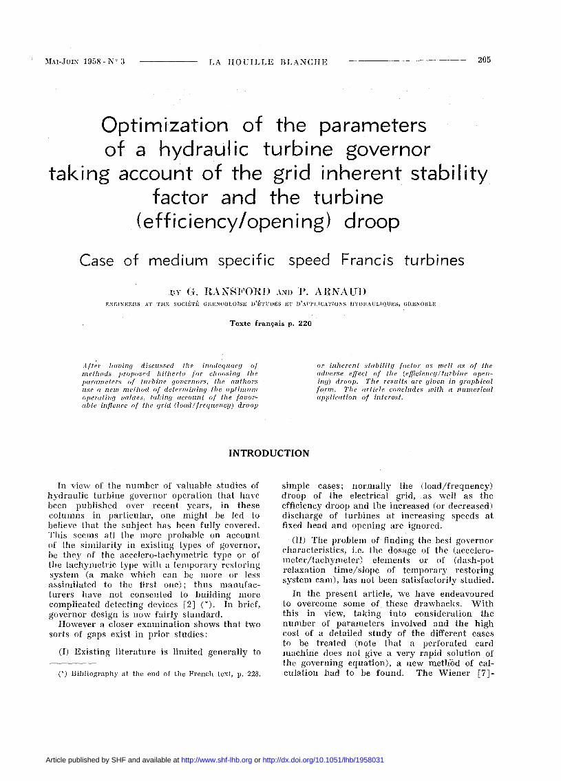
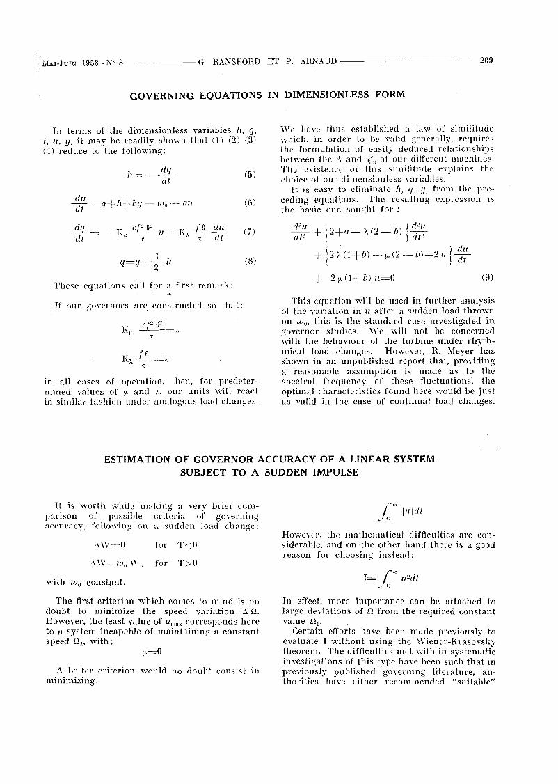
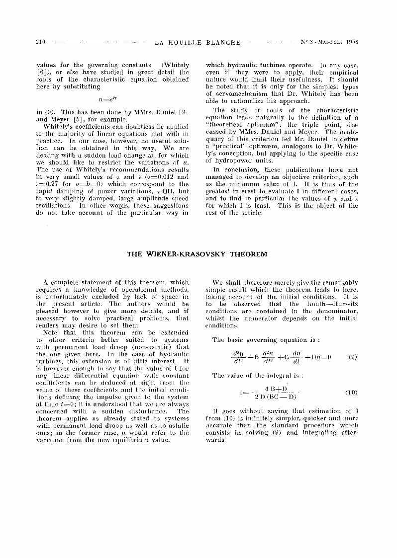
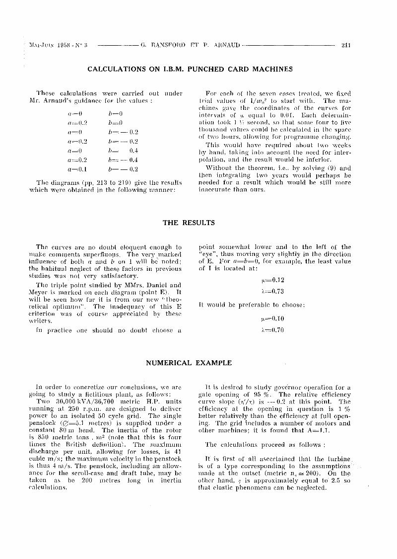
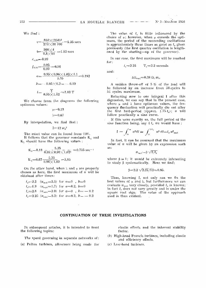
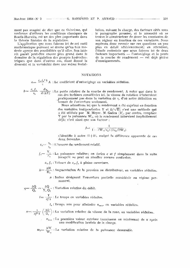
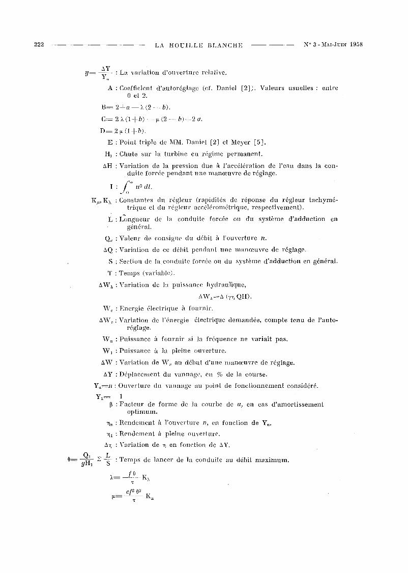
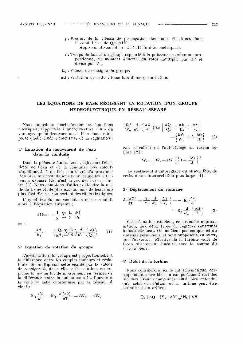
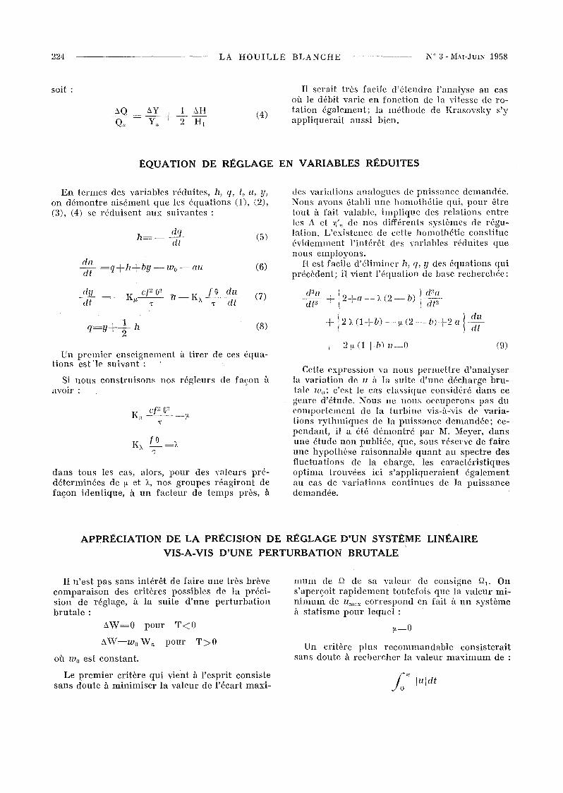
The diagrams (pp. 213 to 219) give the resullswhich were ohtained in the following manner:

These calculations were carried out underMl'. Arnaud's guidance for the values:

a=O

11=-.==0.2

11=0

11=0.2

a=O

a=0.2

a=O.1

b=O

b=O

b=-- 0.2

b= -- 0.2

b= -- 0.4

b= - 0.4

b=-0.2

For each of the seven cases treated, wc fixedtrial values of Ilmo" to starl with. The ma­chines gave the coordinates of the curves forintervals of !J. equal to 0.01. Each determin­ation look J IIi second, so that senne foUt· to fivethousand values could he calculated in the spaceof two hours, allowing for programme changing.

This would have required ahout t"Wo weekshy hand, taking into account the need for inter­polation, and the result would he inferior.

vVithout the theorem, i.e., hy solving (9) andthen integrating two years would perhaps beneeded for a resuIt vV'hich would he still moreinaccurate than ours.

THE RESULTS

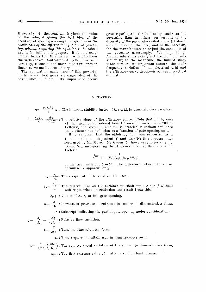
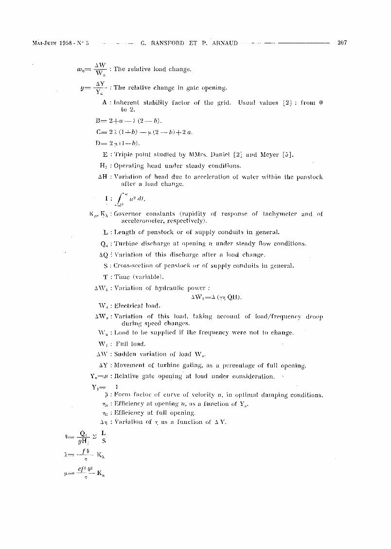
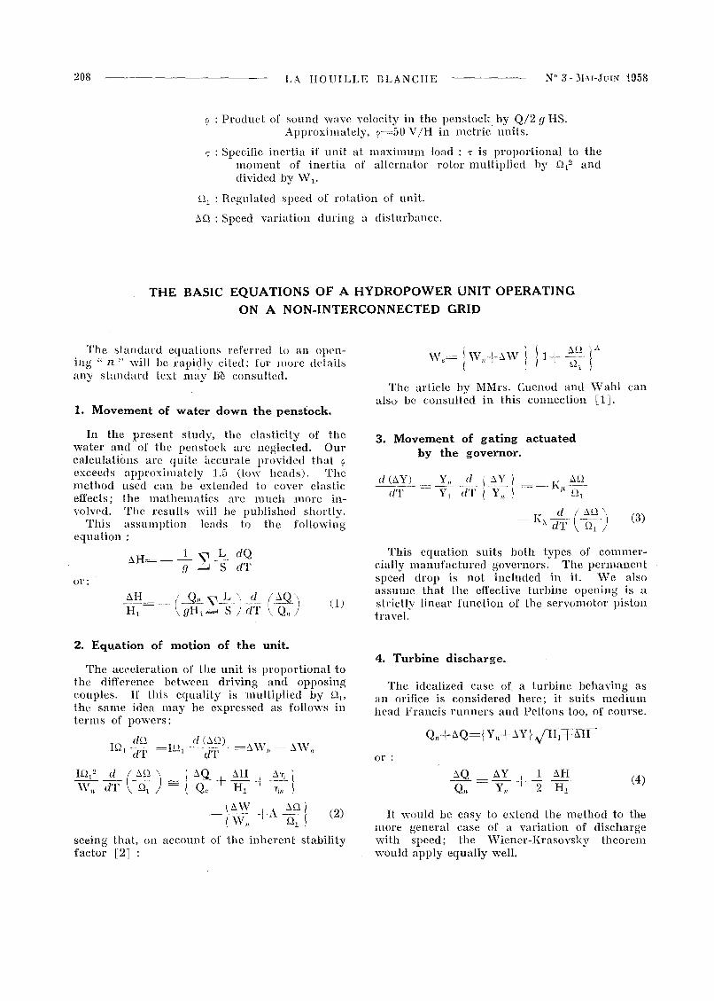
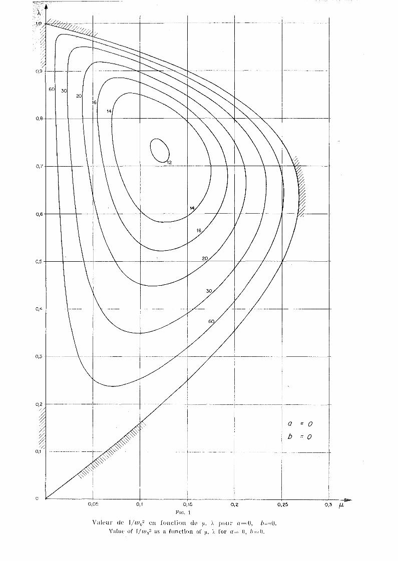
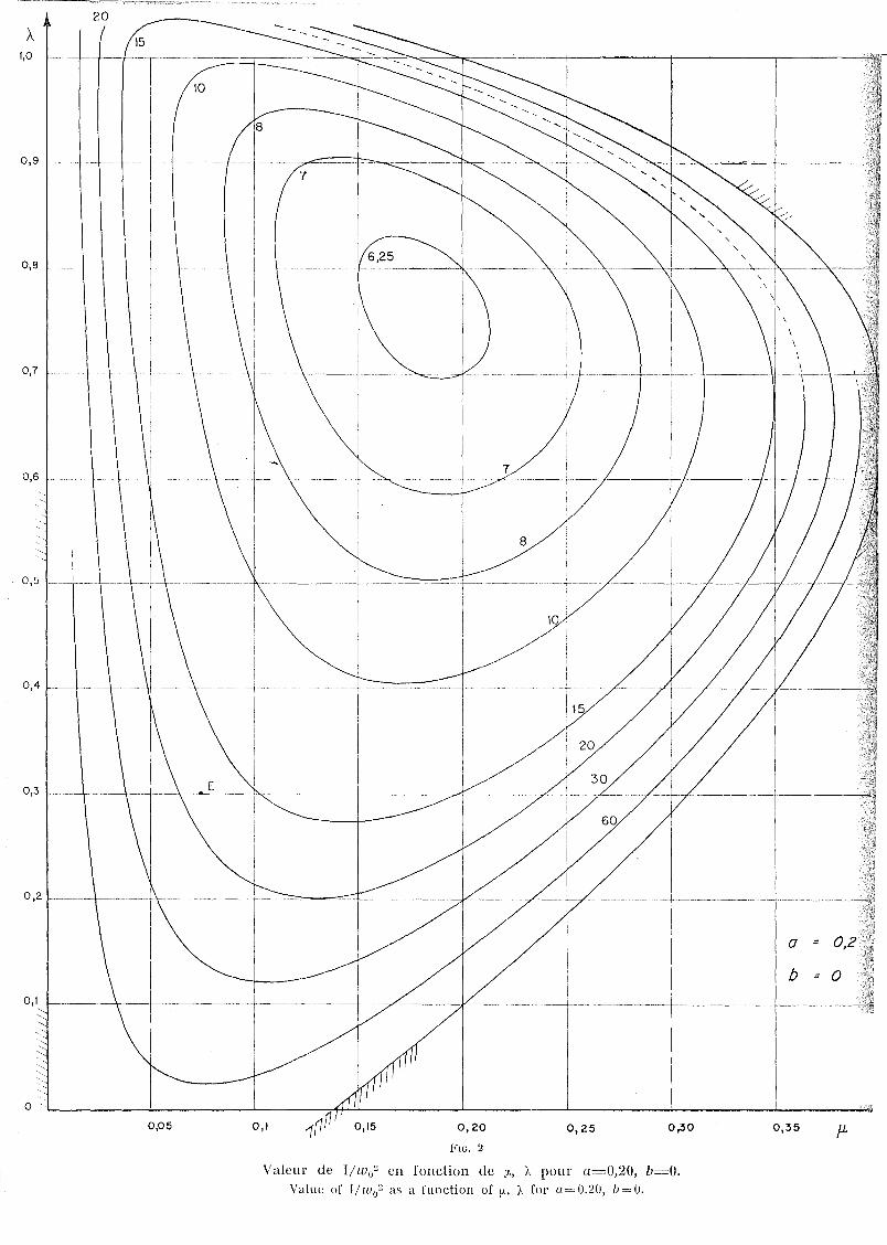
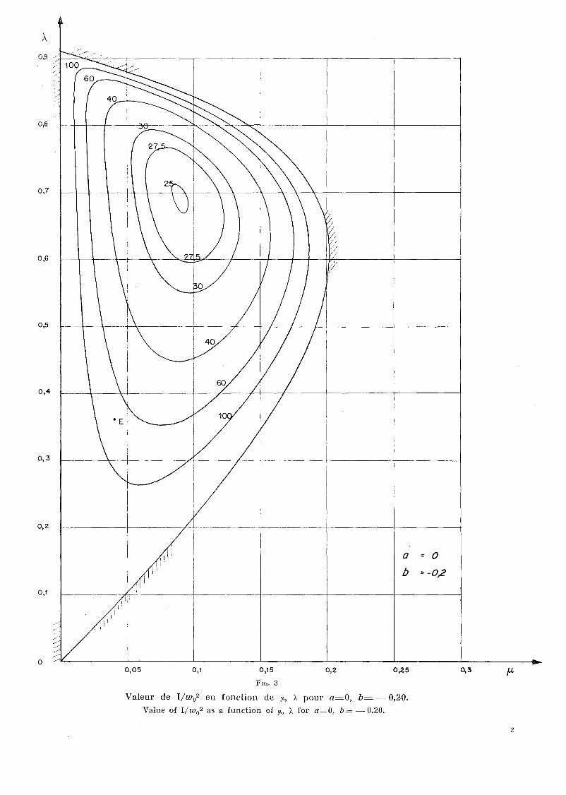
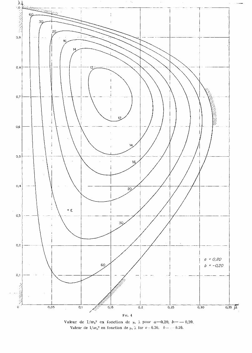
The curves are no doubt eloquent enough tomake comn}ellis supedluo~lS. The verY.luarkedinfluence of both a and b on 1 will be noted;the habituaI neglect of these factors in previousstudies was not very satisfactory.

The triple point studied by MMrs. Daniel andMeyer is marked on each diagram (point E). Ilwill he seen how far il is from our new "theo­retical optimum". The inadequacy of this Ecriterion was of course appreciated by thesewriters.

[n practice one should no douht choose a

point somewhat lower and to the left of the"eye", tlms moving very slightly in the directionof E. For lI=b=O, for example, the least valueof 1 is located at:

p.=0.12

À=0.73

It would be preferable to choose:

p.=0.10

),=0.70

NUMERICAL EXAMPLE

In order to concretize our cone1usions, wc aregoing to study a fietitious plant, as follows:

Two 30,000 kVA/36,700 meIric H.P. unitsrunning at 250 r.p.m. are designed tü deIiverpower to an isolated 50 cycle grid. The singlepenstock (0=5.1 metres) is suppIied under aconstant 80 m head. The inertia of the rotoris 850 metric tons. m 2 (note that this is fourtimes the British definition). The maximumdischarge pel' unit, allowing for lüsses, is 41cuhic mis; the maximum velocity in the penstockis thus 4 mis. The penstock, inc1uding an aIlow­ance for the scroll-case and dran tube, may betaken as be 200 metres long in inertiacalculations.

lt is desired tü study govèrnor operation for agate openingof 95 %' The relative efficiencycurve slope ('r(h) is -- 0.2 at this point. Theefficicncy at the opening in question is 1 %better relatively than the efficiency at full open­ing. The grid inc1udes a number of motors andother machines; it is found that A=1.l.

The calculations proceed as follows :

If is first of all ascertained that the turbineis of a type corresponding to the assumptionsmade at the outset (metric Il,, == 200). On theother hand, ç is approximately equal to 2.5 sothat elastic phenomena can he negleeted.

212 LA HOUILLE~LANCHE N° 3 - MAI-JUIN 1958

In faet, il can be assumed that the maximumvalue of II will be given by an expression such

1',,=2.2 secondsl,,=2.25

A sudden throw-ofI of 5 % of the load willbe followed by an increase from 50 cycles to51 cycles maximum.

Returning now to our integral 1 artel' thisdigression, we can say that in the present case,yvhere \J. and À have optimum values, the fre­([uency fluctuation will practically die out artel'the first half-period (approx. 1.75 l,,); II willfollow practically a sine curve.

If this were exacUy so, the full period of thesine function being, say 4 l" we would have:

and:

The value of l" is litUe influenced by thechoice of \J.; however, when \J. exceeds the opti­mum, the period of the suceeeding oscillationsis approximately three times as great as l" givenpreviously (the first quarter oscillation is length­ened by the starting-up of the governor).

In our case, the first maximum will be reachedfor:

We find :

850X(250)2'1"= 5.35 secs

270X36700

n= 200X 4 1 09v 9.8X80 = . ~ secs

fi. ·0.13

À~0.67

t l' 1.0.''''r= 0 <)/'; 1 09".. oX· ~

/. (1.~)5 0 9(jO,\)f,= 0.99 = ... )

a= 0.95XO.~}6~1.02Xl.l 0.H)25.3b

b=- 0.95XO.2= - 0.19

By interpolation, wc find that:

I=,12wo2

The exact value can I)e found from (10).It follows that the governor constants K,< and

K,\ should have the following values:

vVe choose from the diagrams the followingoptimum values:

=0.735 sec-!as:

where ~ == 1; il would he extremely interestingto study ~ systematically. Here we find:

On the other hand, when ), and fi. are properlychosen as here, the first maximum of II wiII beobtained artel' times:

t,,=2.3 (1lIllax=2.:3) for a=O , b=O

t,,=1.9 (1l,"ax=1.7) for a=0.2, b=O

l,,=2.8 (llmax=3Jl) for a=O , b=-0.2

t,,=2.25 (llll,ax=2.2) for a=0.2, b= -- 0.2

~=2.2 V2.25/12=0.95.

Thus, knowing l, not only can we fix thebest values of !Jo and )" but furthermore we canevaluate lllllax very closely, provided l" is known;in fact ln does not vary greatly and is U1Hler thesquare root sign. The value of the approachused is thus evident.

CONTINUATION OF THESE INVESTIGATIONS

In subsequent articles, il is intended to treatthe following topics:

The speed governing in separate networks of:

(a) Pelton turbines, allowance being made for

elastic effects and the inherent stabilityfactor.

(b) High-head Francis turbines, including elasticand efficiency eil'eets.

(c) Low-head turbines.

14

----------- -----------------7'-c __I- /_

1

16

0,8

0,6+--+--+---1 \----+----t' -------1V---~'---+f__~-+_-_t-___jW--_+

0,4 f-----\

0,5 +---+--+-+----\-----t-------t-------'=r----t-r---r--{------"t

0,3 -

--- - ---- -------------------- -------------1------------1-------- ----------------1--------- ------- -

0=0

b = 0

° 0,05 0,1 0,15

FIG. 1

0,2 0,25 0,3 f1-

Valeur dc l/wo~ cn fondion de (J., J_ pour a=O, b=,"O,Value of Ijw(? as a function of (J., ), for ({= 0, b=dl,

8

7

0,350,300,250,200,10,05

-\-------+-~~--------_._--~----+--------~-0,1

0,2 _

°

20

15

0,3

0, 4 ~__.__+-.-.----,l----.... -\-- _

0,6

0,7

0,5

0,8

0,9

1,0

FIG. 2

Valeur cie I/w()~ en fonction de fi., ), pOlir (/=0,20, b=O.Value of Il w()~ as a function of Il,, À for a 0.20, b = O.

À

0;3

0,8

0,7

0,6

0,5

0,4

0,3

0,2

1

I------~-----

-----,-----.----l

------------+-------j-------t

! ..... --------------- ---I-------------·--------------j-------j

0,1

°

1---------..'1T+----------+----------j---------j---

a ::: 0

b :::-o~

0,05 0,1 0,15

FIG. 3

0,2 0,25 0,3

Valeur de I/wo2 en fonction de p., ), pour a=O, b= - 0,20.

Value of Il W()2 as a function of p., ), for a= 0, b = - 0.20.

2

0,35 fL0,300,25

,/ .....- ..- --1--/'·-'--·--·--"'- ---- ...-- .....-.-..-.---.--

0,2

12. -__..

0,1

• E

/

If------'...--t-------l-------?L+-----·--····,I-··---f---··f --.-.--- -/-- ------

0,05

I--t-----·------+-------l------/---l---;l-------+------··..-----t-·-------

f-t,~.·~6"7'(Tr;r-r-··-··· ··,-·-·······--··-·-·-·---···T---·-------,-----·---,--····-----,---..--..---.-,---------,

0,1 --

0,3 ·--------\-···---.----\,----··-r------\--c-----/

0,8-·-

0,7 .-- -- ----···---··\---··\---·-I--·--\------/--

0,6 I---+---+--;--.I-~-\---'i---.---+----

0,5

FIG. 4

Valeur de I/wo2 en fonction de [1., ), pour a=0,20, b= - 0,20.

Valeur de I/wo2 en fonction de [1., J, for 0=0.20, b= -- 0.20.

i1

"--+-----1l,

1---~----~-"~-~----j~~------i

0,7

0,6 f--I---+-\--+\---

0,8

0,5 f-~f------'2lt--+-------A-----f--/'--+---------j

0,3

0,2 f------+----f-----j-------+--------j

a:: 0

b=-Q4

~-__L___~__L___I_° 0,05 0,1 0,15 0,2 fL

FIG. 5

Valeur de I/wo~ en fonction de iL, ), pour a=O, b= - 0,40.Value of I/ wo2 as a function of iL, j, for a=O, b= ~ 0.40.

jO,8é>----1--

0,7 I-------'f--

0,6 I------~

0,5 I-----+-~~--++

0,4 I----------\--t---\_-

0,31--------\+-------'1------

1---------1---~~~----

0,25 f-L0,20,1 L:::-r-

0,05

0,1

FIG. 6

Valeur de I/wo2 en fonction de !J., }, pour a=0,20, b= - 0,40.Value of I/ wo2 as a function of !h, À for a=0.20, b= - 0.40.

60

0,4

0,8

0,3 r--------\r---f--------+--------b"-------t'--+------+-------+

0,2 1--------+-------+--------+-7'----------j-------+-"------+

a = 0,/

/

0,1 ~ J____I---:~o.-----'-'-_+-----_+_-----+--b.-=--O'-'-2-_+1

o'/"-------L-~~----l---------J------...L--------l.------..l---....0,1 0,15 0,20 0,25 0,30 fi.

FIG. 7

Valeur de I/wo2 en fonction de [1, J, pour a=0,10, b= - 0,20.Value of I/ wo2 as a function of {J., J. for a=0.10, b= - 0.20.

220 LA HOUILLE BLANCHE N° 3 -MAI-JUIN 1958

La détermination des caractéristiques optimad'un régleur hydraulique,

compte tenu de l'autoréglage et de la pentede la courbe de rendement

Cas des turbines Francis de ns

PAR G. RAN8FÛRD l~T P. ARNAUD

moyen

INGÉNIEURS A LA SOCIÉTÉ GIIENOBLOlSE n'fèTliDES ET n'APPLICATIONS HYDIIAULlQUES, GI\ENOBLE

English text p. 205

,Après avoir mis en évidence l'insullisance desmoyens olTerls 'dans la liltératllre existantepour choisir les cons lan/es des régleurshydrauliques, les ollteZlrs utilisent Zlne nozwelleméthode lJOllr déterminer les valeurs optima,('OllllJte /enu de l'inf7l1enee, favorable, de l'auto-

INTRODUCTION

réglage el de celle, défavorable, d'unc penlelombanle de la courbe de rendemenl, Les résul­tals détaillés, présentés SOzlS forme de sept ara­phiqlles, sont concrélisés par llTle applicationnumérique.

Les très belles études qui ont été consacréesces dernières années, dans ces colonnes notam­ment, au comportement des régleurs hydrauli­ques, pourraient amener à croire que le sujetn'est désormais susceptible d'aucun approfon­dissement retentissant. Le fait que la conceptionmême de ces régleurs - essentiellement du typeà détection accélérotachymétrique, auquel le typetachymétrique à asservissement temporaire peutêtre plus ou moins assimilé - paraît figée, lesconstructeurs n'ayant pas voulu réaliser des sys­tèmes de détection plus compliqués [2J, n'inci­terait guère à penser que des résultats nouveauxpuissent être escomptés dans ce domaine.

Cependant, lorsqu'on regarde les choses deplus près, on constate l'existence de deux sortesde lacunes:

1 0 La littérature existante se borne en gene­l'al à traiter des cas très simples; on exclut habi­tuellement l'influence de l'autoréglage du réseauélectrique, de la pente de la courbe de rendement,

de l'appel de débit des turbines en cas d'aug­mentation de vitesse, etc.

2° La question de la détermination du dosageoptimum de chacun des éléments (accéléromè­tre/tachymètre), ou (temps de relaxation dudash-pot/pente de la came du statisme tempo­raire), n'a pas été trairée de façon adéquate.

Dans le présent article, nous tentons de remé­dier à certaines de ces insuffisances. Pour cela,vu le nombre des facteurs à prendre en considé­ration ct le coût élevé d'une étude détaillée desdifférents cas (la solution des équations de réglagen'est pas très rapide sur une machine à calculerà cartes perforées), il a fallu vraiment trouverune nouvelle méthode d'analyse. Le théorème deWiener [7]-Krasovsky [4], qui permet de déter­miner l'intégrale caractérisant au mieux la qua­lité de la régulation A PABTIR DES COEFFICIENTS DE

L'I~QUATION DIFFÉBENTIELLE DE BÉGLAGE, SANS

QU'ON SOIT OBLIGÉ D'EXPLICITER LA SOLUTION DE

CETTE ÉQUATION, remplit ce rôle; il ne serait sûre-

MAI-JUIN 1958 - N° 3 G. RANSFûRD ET P. ARNAUD ------------ 221

ment pas exagéré de dire que ce théorème, quirenferme d'ailleurs les conditions classiques deRouth-Hurwitz, est un des plus importants dansla théorie linéaire de la régulation.

L'application que nous faisons ici de cet outilmathématique puissant ne donne qu'un très mo­deste aperçu des possibilités qu'il ofIre. Son inté­rêt paraît peut-être encore plus grand dans ledomaine de la régulation des groupes hydroélec­triques que dans d'autres cas, étant donné ladiversité et la variabilité dans UIle même instal-

lation, suivant la charge, des facteurs cités sousle paragraphe premier, et la nécessité où setrouve le constructeur de doser les constantes deson régleur en fonction de ces variations. Nousespérons donc revenir sur ces questions un peuplus en détail ultérieurement; en [lttendant,l'étude restreinte que nous faisons ici de deuxfacteurs importants - l'autoréglage et la pentede la courbe de rendement - est déjà pleined'enseignements.

NOTATIONS

a= CI' fn2

0 A : Le coefficient d'autoréglage en variables réduites.'i:

b= Cnln'~n

d'~n

d (ClY) : La pente relative de la courbe de rendement. A noter que dans lecas des turbines considérées ici, la vitesse de rotation n'intervientpratiquement pas dans la variation de .~, d'où notre définition en

"'termes de l'ouverture seulement.Nous admettons ici que le rendement a été exprimé en fonction

des variables indépendantes Y et ü/\iH; c'est une méthode quia été utilisée par M. Meyer. M. Gaden [3J, par contre, remplaceY par la puissance Wh' où le rendement intervient implicitementdéjà; c'est ainsi que son facteur:

. 11= --.------..~.--------. 1 '- (W l'/~n) (o'~,joWh)

s'identifie à notre Cl +b), malgré la différence apparente de cesdeux formules.

Cn== _'~L : L'inverse du rendement relatif.·rJJI.

fll= ~ : La puissance relative; on écrira C et f simplement dans la suiteCil lorsqu'il ne peut en résulter aucune confusion.

CI' fI : Valeurs de C,,, fn à pleine ouverture.

lz= ~~.: Augmentation de la pression au distributeur, en variables réduites.

n : Indice désignant l'ouverture partielle considérée en régime per­manent.

q- ClQ_~ : Variation relative du débit.- Qn - YII QI

T1= -1-'- : Lc temps en variables réduites.

C 0

ln : Temps mis pour atteindre l1mllx ' en variables réduites.

't' ( ClQ)' 1 . t' l t' l' d11.= -- -0 : Al vanalOn re nIve (e vItesse e la roue, en variables réduites ..Cf2 0 ~"l

I1. mux : La premlere valeur extrême (maximum ou minimum) de II aprèsune modification brutale de la charge.

nvWo= 'N : La variation relative de la puissance demandée.

l'

222 LA HOUILLE BLANCHE

~Yy= -- : La variation d'ouverture relative.Y"

N° 3 - MAI-JUIN 1958

A : Coefficient d'autoréglage (cf. Daniel [2]). Valeurs usuelles: entreo et 2.

B= 2+(1 -), (2 --- b).

C= 2), O+b) - fi. (2 - b)+2 (1.

D= 2 fi. O+b).

E : Point triple de MM. Daniel [2] et Meyer [5].

Hl : Chute sur la turbine en régime permanent.

ÂH : Variation de la pression due à l'accélération de l'eau dans la con­duite forcée pendant une manœuvre de réglage.

1: j'" 1(2 di.JoRf" R

À: Constantes du régleur (rapidités de réponse du régleur tachymé­

trique et du régleur accélérométrique, respectivement) ....

L : Longueur de la conduite forcée ou du systèn1e d'adduction engénéral.

Qn : Valeur de consigne du débit à l'ouverture I/.

ÂQ : Variation de ce débit pendant une manœuvre de réglage.

S ; Section de la.eonduite foreée ou du système d'adduetion en général.

T : Temps (variable).

ÂWh : Variation dc la puissance hydraulique,

ÂW,,=Â (n QH).

vVe: Energie électrique à fournir.

 \V e : Variation de l'énergie électrique demandée, compte tenu de l'auto-réglage.

\V" : Puissance à fournir si la fréquence ne variait pas.

W 1 : Puissance à la pleine ouverture.

 vV : Variation de vV" au début d'une manœuvre de réglage.

Ây : Déplacement du vannage, en % de la course.

Y,,=Il : Ouverture du vannage au point de fonctionnement considéré.

Yl = 1~ : Facteur de forme de la courbe de u, en cas d'amortissement

optimUlU.

"1]" : Rendement à l'ouverture Il, en fonction de Y".

"1]1 : Rendement à pleine ouverture.

Â'~ : Variation de "1] en fonetion de  Y.

Cl Ql" L , 1v- -- ~ -s : reml)s de ancer de la conduite au débit maximum.- gHl

fa),= ---RÀ

'! '

LVL\I-JUIN 1958 - N° 3 ·G. HANSFûRD ET P. AHNAUD ------

9 : Produit de la vitesse de propagation des ondes élastiques dansla conduite et de Q/2 g HS.

Approximativement, ?=50 VIH (unités métriques).

't' : Temps de lancer du groupe rapporté à la puissance maximum; pro­portionnel au moment d'inertie du rotor multiplié par 0 1

2 etdivisé par W].

n] : Vitesse de consigne du groupe.

.M2 : Variation de cette vitesse lors d'une perturbation.

223

LES EQUATIONS DE BASE RÉGISSANT LA ROTATION D'UN GROUPE

HYDROELECTRIQUE EN RÉSEAU SEPARÉ

Nous rapp~lons succinctement les équationsclassiques, rapportées à une ouverture « n » duvannage, qu'on trouvera aussi bien dans n'im­porte quelle étude élémentaire de la régulation:

1012

d 1 .M2. ')\V,~ dT \ 0]

(2)

1° Equation du mouvement de l'eaudans la conduite

Dans la présente étude, nous négligeons l'élas­ticité de l'eau et de la conduite; nos calculss'appliquent, à un très bon degré d'approxima­tion près, aux installations pour lesquelles le fac­teur ? dépasse 1,5; c'est le cas des basses chu­tes [2]. Nous comptons d'ailleurs étendre la mé­thode à une étude plus exacte, mais de beaucoupplus fastidieuse, comportant des effets élastiques.

L'hypothèse du mouvement en masse condui talors à l'équation suivante:

tlH=-~ ~ ~ dQg L.J S dt

ou

(1)

2° Equation de rotation du groupe

L'accélération du groupe est proportionnelle àla différence entre les couples moteurs et résis­tants. Si, multipliant cette égalité par la valeurde consigne 0] de la vitesse de rotation, on ex­prime la même loi de mouvement en termes dela différence entre la puissance utile fournie àla roue et celle consommée par le réseau, ilvient:

10 dn =10]. d (ilQ) =ilW,. - ilW,--] dl' dl' ' 0

car, en raison de l'autoréglage en réseau sé­paré [2]

Le coefficient d'autoréglage est susceptible, dul'este, d'une interprétation plus large [1].

3° Déplacement du vannage

d (ilY)

dT

(3)

Cette équation convient, en première approxi­mation, aux deux types de régleurs construitsindustriellement. On ne tient pas compte ici dustatisme permanent, et nou~ supposons, en outre,que l'ouverture effective de la turbine varie defaçon strictement linéaire avec la course duservo-moteur.

4° Débit de la turbine

Nous considérons ici le cas schématique, cor­respondant assez bien au comportement réel desturbines Francis moyennes, ainsi, bien entendu,qu'à celui des Pelton, où la turbine peut êtreassimilée à un orifice :

224 LA HOUILLE BLANCHE N° 3 - MAI-JUIN 1958

soit :

6.Q

Q"

1 6.H--2 Hl

(4)

Il serait très facile d'étendre l'analyse au casoù le débit varie en fonction de la vitesse de ro­tation également; la méthode de Krasovsky s'yappliquerait aussi bien.

EQUATION DE REGLAGE EN VARIABLES RÉDUITES

En termes des variables réduites, h, q, t" H, y,on démontre aisément que les équations (1), (2),(3), (4) se réduisent aux suivantes:

h=- dq_dt

(5)

(6)

des variations analogues de puissance demandée.Nous avons établi une homothétie qui, pour êtretout à fait valable, implique des relations entreles A et '~'It de nôs différents systèmes de régu­lation. L'existence de celte homothétie constitueévidemment l'intérêt des variables réduites quenous employons.

Il est facile d'éliminer h" q, Y des équations quiprécèdent; il vient l'équation de base recherchée:

Cette expression va nous permettre d'analyserla variation de Il il la suite d'une décharge bru­tale W o; c'est le cas cl assique considéré dans cegenre d'étude, Nous ne nous occuperons pas ducomportement de la turbine vis-à-vis de varia­tions rythmiques de la puissance demandée; ce­pendant, il a été démontré par M. Meyer, dansune étude non publiée, que, sous réserve de faireune hypothèse raisonnable quant au sp'ectre desfluctua lions de la charge, les caractéristiquesoptima trouvées ici s'appliqueraient égalementau cas de variations continues de la puissancedemandée.

d!! = _ K cf202 11 _ K ~ du (7)

dt iL '" À 't' dt

Un premier enseignement ù tirer de ces équa­tions est 'le suivant:

Si nous construisons nos régleurs de façon àavoir:

cf2 02Ku -----.--., =!J,

" 't' '

dans tous les cas, alors, pour des valeurs pré­déterminées de !L et )" nos groupes réagiront defaçon identique, à un facteur de temps près, à

(J'l,Il + \'LL __ ) ('> ---1) L!F,II,dt;] (~Ia ,~ > \ dt2

\ l dll,2), (1+b) - fi. (2,- b)-1-2 a dt

2!J,(1+b) 11=-=0 (9)

APPRÉCIATION DE LA PRÉCISION DE REGLAGE D'UN SYSTEME LINÉAIREVIS-A.VIS D'UNE PERTURBATION BRUTALE

Il n'est pas sans intérêt de faire une très brèvecomparaison des critères possibles de la préci­sion de réglage, à la suite d'une perturbationbrutale:

6.W=O pour 1'<0

6.W=wo W" pour 1'>0

où W o est constant.

Le premier critère qui vient à l'esprit consistesans doute à minimiser la valeur de l'écart maxi-

BlUm de n de sa valeur de consigne nI' Ons'aperçoit rapidement toutefois que la valeur mi­nimum de llmax correspond en fait à un systèmeà statisme pour lequel:

!L=O

Un critère plus recommandable consisteraitsans doute à rechercher la valeur maximum de :

lVL\I-JUIN 1958 - N° 3 -----G. HANSFOHD ET P. AHNAUD -------------- ..-------- 225

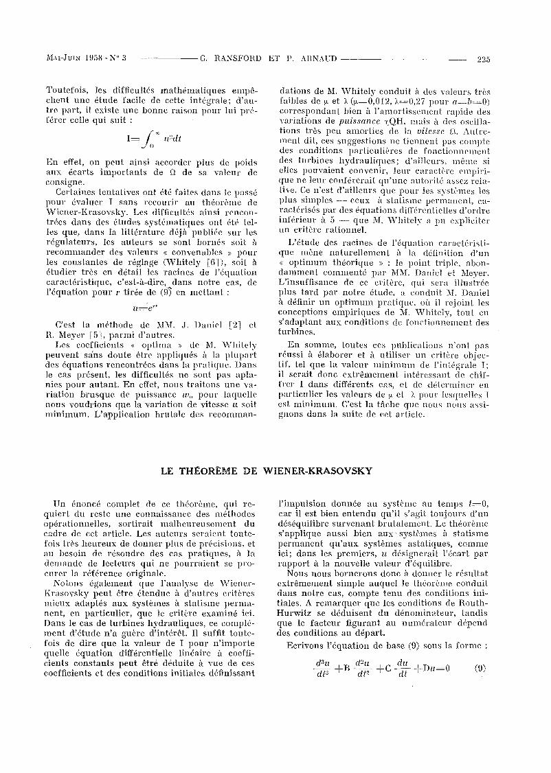
Toutefois, les difficultés mathématiques empê­chent une étude facile de cette intégrale; d'au­tre part, il existe une bonne raison pour lui pré­férer celle qui suit :

1= {'" u~dtJoEn effet, on peut ainsi accorder plus de poidsaux écarts importants de 0 de sa valeur deconsigne.

Certaines tentatives ont été faites dans le passépour évaluer 1 sans recourir au théorème devViener-Krasovsky. Les difficultés ainsi rencon­trées dans des études systématiques ont été tel­les que, dans la littérature déjà publiée sur lesrégulateurs, les auteurs se sont bornés soit àreconunander des valeurs « convenables » pourles constantes de réglage (Whitely [6]), soit àétudier très en détail les racines de l'équationcaractéristique, c'est-à-dire, dans notre cas, del'équation pour l' tirée de (9) en mettant:

u -erl

C'est la méthode de MM..f. Daniel [2] elH.. Meyer [5]. parmi d'autres.

Les coefficients « optima » de M. vVhitelypeuvent sans doute être ~lppliqués à la plupartdes équations rencontrées dans la pratique. Dansle cas présent, les difficultés ne sont pas apla­nies pour autant. En effet, nous traitons une va­riation brusque de puissance W o pour laquellenous voudrions que la variation de vitesse II soitminimum. L'application brutale des recomman-

dations de M. vVhitely conduit à des valeurs trèsfaibles de Il. et ), ([J.=0,012, ),=0,27 pour a=b=O)correspondant bien à l'amortissement rapide desvariations de puissance -r,QH, mais à des oscilla­tions très peu amorties de la vitesse n. Autre­ment dit, ces suggestions ne tiennent pas comptedes conditions particulières de fonctionnementdes turbines hydrauliques; d'ailleurs, même sielles pouvaient convenir, leur caractère empiri­que ne leur conférerait qu'une autorité assez rela­tive. Ce n'est d'ailleurs que pour les systèmes lesplus simples - ceux à statisme permanent, ca­ractérisés par des équations ditrérentielles d'ordreinférieur à 5 -.--- que M. vVhitely a pu expliciterun critère rationnel.

L'étude des racines de l'équation caractéristi­que mène naturellement à la définition d'un« optimum théorique » : le point triple, abon­damment COlTl1nenté par MM. Daniel et Meyer.L'Insuffisance de ce critère, qui sera illustréeplus tard par notre étude, a c·onduit M. Danielà définir un optimum pratique, où il rejoint lesconceptions empiriques de M. "\Vhitely, tout ens'adaptant aux eonditions de fonctionnement desturbines.

En somme, toutes ees publieations n'ont pasréussi à élaborer et à utiliser un critère objee­tif, tel que la valeur minimum de l'intégrale 1;il serait donc extrêmement intéressant de chif­frer 1 dans différents cas, et de déterminer enpartieulier les valeurs de [J. et ), pOlI r lesquelles 1est minimum. C'est la tâche que nous nous assi­gnons dans la suite de cet article.

LE THÉORÈME DE WIENER.KRASOVSKY

Un énoncé complet de ce théorème, qui re­quiert du reste une connaissance des méthodesopérationnelles, sortirait malheureusement ducadre de cet article. Les auteurs seraient toute­fois très heureux de donner plus de précisions, etau besoin de résoudre des cas pratiques, à lademande de lecteurs qui ne pourraient se pro­curer la référenee originale.

Notons également que l'analyse de "YViener­Krasovsky peut être étendue à d'autres critèresmieux adaptés aux systèmes à statisme penna­!lent, en particulier, que le critère examiné iei.Dans le cas de turbines hydrauliques, ce complé­ment d'étude n'a guère d'intérêt. Il suffit toute­fois de dire que la valeur de 1 pour n'importequelle équation différentielle linéaire à eoeffi­cients constants peut être déduite à vue de eescoefficients et des eonditions initiales définissant

l'impulsion donnée au système au temps t=O,car il est bien entendu qu'il s'agit toujours d'undéséquilibre survenant brutalement. Le théorèmes'applique aussi bien aux' systèmes à statismepermanent qu'aux systèmes astatiques, commeici; dans les premiers, II désignerait l'éeart parrapport à la nouvelle valeur d'équilibre.

Nous nous bornerons donc à donner le résultatextrêmement simple auquel le théorème eonduitdans notre cas, eom_pte tenu des conditions ini­tiales. A remarquer que les eonditions de H.outh­Hurwitz se déduisent du dénominateur, tandisque le facteur figurant au numérateur dépenddes conditions au départ.

Ecrivons l'équation de base (9) sous la forme:

d3 zz d~ll 1 du 1 _

dta +B dt2 TC dt TDu-O (9)

226 LA HOUILLE BLANCHE Nu ;1 - MAI-JUIN 1958

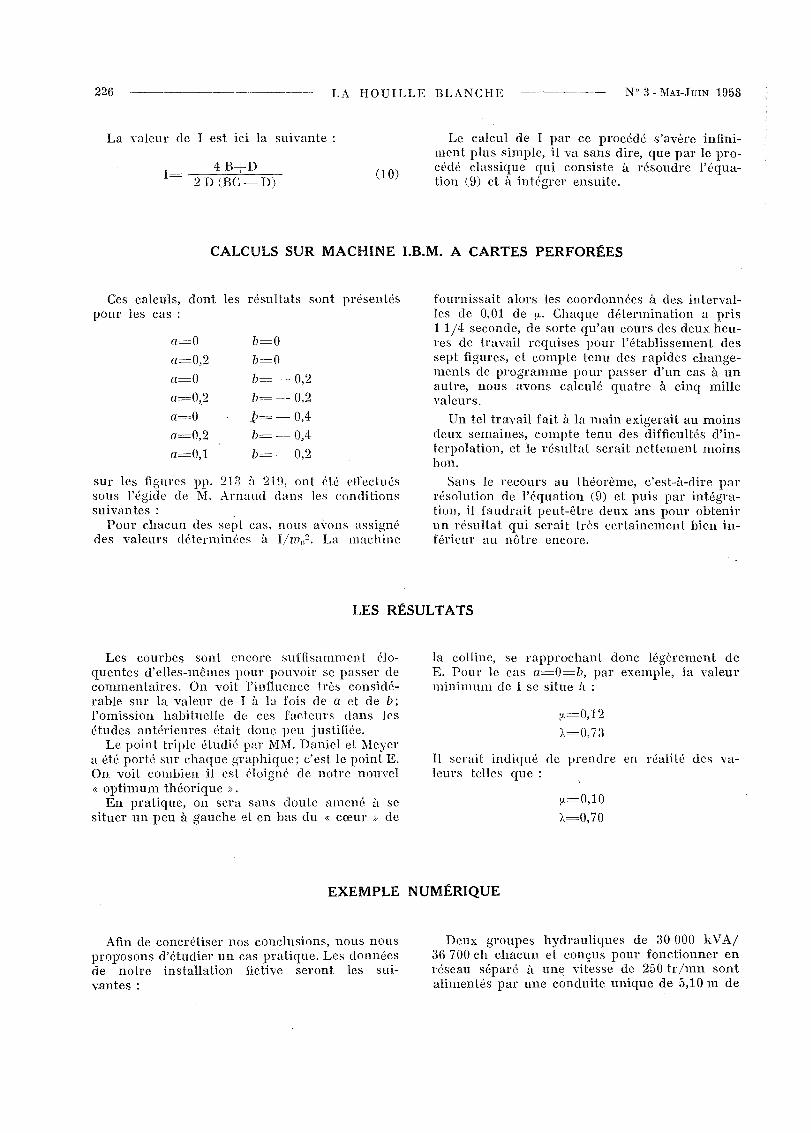
La valeur de 1 est ici la suivante:

4B+D1= 2 D (BC-D)

(10)

Le calcul de 1 par ce procédé s'avère infini­men t plus simple, il va sans dire, que par le pro­cédé classique qui consiste à résoudre l'équa­tion (9) et à intégrer ensuite.

CALCULS SUR MACHINE I.B.M. A CARTES PERFORÉES

Ces calculs, dont les résultats sont présentéspour les cas :

sur les figures pp. 21:3 il 21\), ont été etl'eduéssous l'égide cie M. Arnaud dans les conditionssuivantes: .

Pour chaeun des sept eas, nOlis a"ons assignédes valeurs déterminées à I/wo2. La Illaehine

a=O

a=0,2

a=O

a=0,2

a=O(1=0,2

a=O,1

b=O

b=O

b=-0,2b= --- 0,2

»=-0,4

b=-O,4b= ---- 0,2

fournissait alors les coordonnées à des interval­les de 0,01 de p.. Chaque détermination a pris1 1/4 secondc, de sorte qu'au cours des deux heu­res de travail requises pour l'établissement dessept figures, et compte tenu des rapides change­ments de programme pour passer d'un cas à unautre, Ilousavons calculé quatre à cinq millevaleurs.

Un tel travail fait à la main exigerait au moinsdeux semaines, eompte tenu des difficultés d'in­terpolation, et le résultat serait nettement moinsbon.

Sans le recours au théorème, c'est-à-dire parrésolution de l'équation (9) et puis par intégra­tion, il faudrait peut-être deux ans pour obtenirun résultat qui serait très eertainement bien in­férieur au nôtre encore.

LES RÉSULTATS

Les eourbes sont encore suffisamment élo­quentes d'elles-mêmes pour pouvoir se passer decommentaires. On voit l'influence très considé­rable sur la valeur de 1 à la fois de a et de b;l'omission habituelle de ces facteurs dans lesétudes antérieures était donc peu justifiée.

Le point triple étudié par MM. Daniel et Meyera été porté sur chaque graphique; c'est le point E.On voit combien il est éloigné de notre nouvel« optimum théorique».

En pratique, on sera sans doute amené il sesituer un peu à gauche et en bas du « cœur» de

la colline, se rapprochant donc légèrement deE. Pour le cas a=O=b, par exemple, la valeurminimum de 1 se situe il :

p.=0,12

),=0,73

Il serait indiqué de prendre en réalité des va­leurs telles que :

p.=0,10),=0,70

EXEMPLE NUMÉRIQUE

Afin de concrétiser nos conclusions, nous nousproposons d'étudier un cas pratique. Les donnéesde notre installation fictive seront les sui­vantes:

Deux groupes hydrauliques de 30000 kVA/36 700 ch chacun et conçus pour fonctionner enréseau séparé à une, vitesse de 250 tr/mn sontalimentés par une conduite unique de 5,10 m de

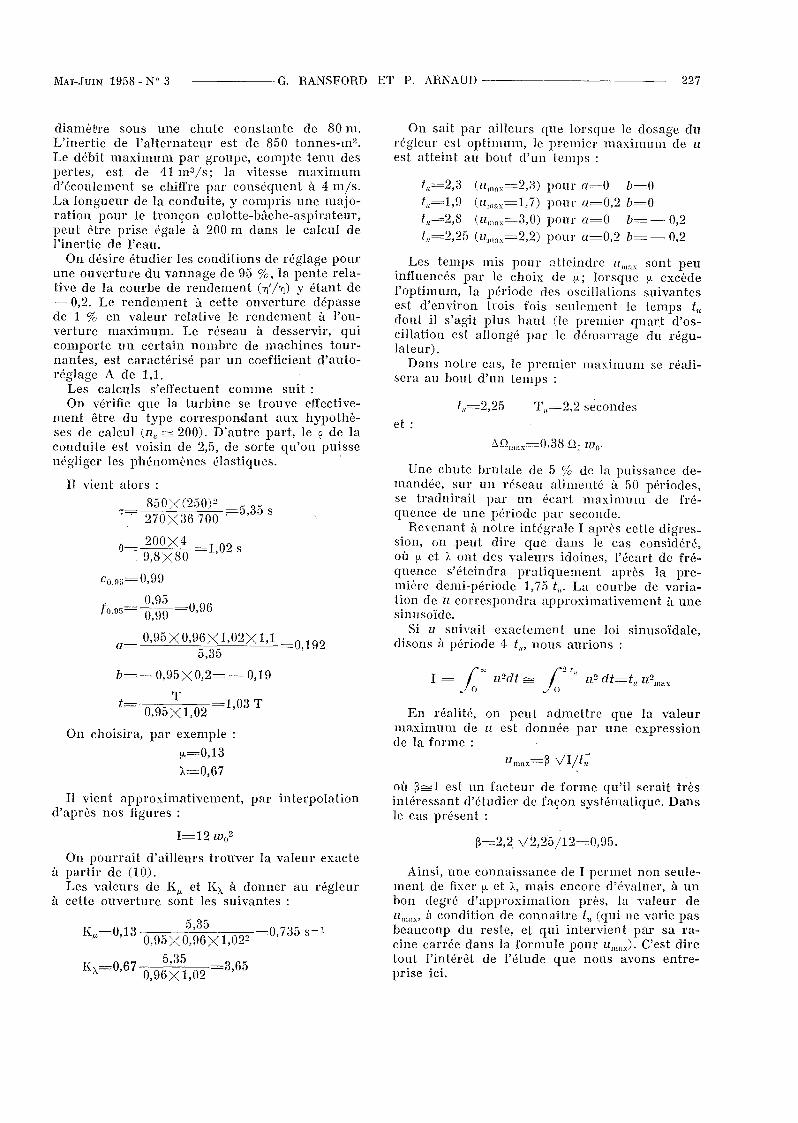
MAI-JUIN 1958 - N° 3 ----- G. RANSFûRD ET P. ARNAUD ------------- 227

et :T,,=2,2 secondes

Une chute hrutale de 5 % de la puissance de­mandée, sur un réseau alimenté à 50 périodes,se traduirait par un écart maximum de fré­quence de une période par seconde.

Revenant à notre intégeale 1 après cette digres­sion, on peu t dire que dans le cas considéré,où iL et J, ont des valeurs idoines, l'écart de fré­quence s'éteindra pratiquement après la pre­mière demi-période 1,75 tu' La courbe de varia­tion de zz correspondra approximativement il unesinusoïde.

Si zz suivait exactement une loi sinusoïdale,disons à période 4 t", nous aurions :

En réalité, on peu t admettre que la valeurmaximum de Il est donnée par une expressionde la forme:

On sait par ailleurs que lorsque le dosage durégleur est optimum, le premier maximum de zzest atteint au hout d'un temps:

t,,=2,3 (zzmax=2,:n pour 0=0 b=Ot,,=1,9 (zzmax=1,7) pour a=0,2 b=Ot,,=2,8 (Zlmax=3,0) pOUl' 0=0 b= - 0,2t,,=2,25 (zzmax=2,2) pour a=0,2 b= - 0,2

Les temps mis pour ntleindre lima" sont peuinfluencés par le choix de p.; lorsque !J. excèdel'optimum, la période des oscillations suivantesest d'environ trois fois seulement le temps tu.dont il s'agit plus haut (le premier quart d'os­cillation est allongé par le démarrage du régu­lateur).

Dans notre cas, le premier maximum se réali­sera au bout d'un temps:

On choisira, par exemple:

p.=0,13

1.=0,67

diamèt're sous une chute constante de 80111.L'inertie de l'alternateur est de 850 tonnes-m2.Le débit maximum par groupe, compte tenu despertes, est de 411113/s; la vitesse maximumd'écoulement se chifTre par conséquent à 4 ln/s.La longueur de la conduite, y compris une majo­ration pour le tronçon culotte-bâche-aspirateur,peut être prise égale à 200 111 dans le calcul del'inertie de l'eau.

On désire étudier les conditions de réglage pourune ouverture du vannage de 95 %, la pente rela­tive de la courbe de rendement (.~,h) y étant de--- 0,2. Le rendement à cette ouverture dépassede 1 % en valeur relative le rendement à l'ou­verture maximum. Le réseau à desservir, quicomporte un certain nombre de machines tour­nantes, est caractérisé par un coefficient d'auto­réglage A de 1,1.

Les calculs s'efTectuent connne suit:On vérifie que la turbine se trouve efTective­

ment être du type correspondant aux hypothè­ses de calcul (n s 2 200). D'autre part, le ? de laconduite est voisin de 2,5, de sorte qu'on puissenégliger les phénomènes élastiques.

Il vient alors :

850X(250)2~ ;-5,35 s,~ 270X36 700

200X4 -109o 9,8X80 - , - s

co,9,,=0,99

f - 0,95 -0 ()60,9,,- 0,99 - " )

a 0,95XO,96X1,02Xl,1 =0,1925,35

b=- 0,95XO,2= - 0,19

T 1,03 T0,95X1,02

Il vient approximativement, par interpolationd'après nos figures:

1=12 W()2

On pourrait d'ailleurs trouver la valeur exacteà partir de (10).

Les valeurs de K,u et KÂ à donner au régleurà cette ouverture sont les suivantes:

5,35K 013 0,735 S-l,u=, 0,95XO,96Xl,022

7 5,35 36-KÂ=0,6 0,96X1,02 ' b

où ~:::::::1 est un facteur de forme qu'i! serait trèsintéressant d'étudier de façon systématique. Dansle cas présent:

~=2,2 v2;25712=0,95.

Ainsi, une connaissance de 1 penllet non seule­ment de fixer iL et J., mais encore d'évaluer, à unhon degré d'approximation près, la valeur delima,,' à condition de connaître tu (qui ne varie pasbeaucoup du reste, et qui intervient par sa ra­cine carrée dans la fonnule pour lima,.). C'est diretout l'intérêt de l'étude que nous avons entre­prise ici.

228 LA HOUILLE BLANCHE N° 3 - MAI-JUIN 1958

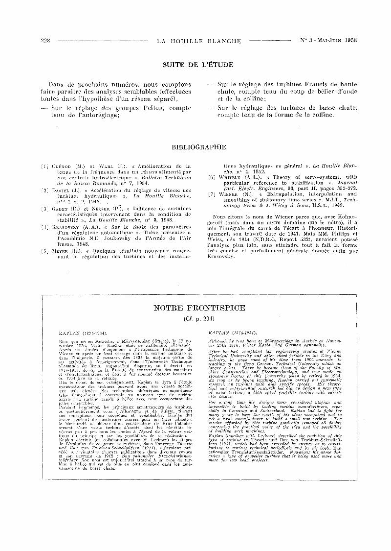
SUITE DE L'ÉTUDE

Dans de prochains numéros, nous comptonsfaire paraître des analyses semblables (effectuéestoutes dans l'hypothèse d'un réseau séparé),

Sur le réglage des groupes Pellon, comptetenu de l'autoréglage;

Sur le réglage des turbines Francis de hautechute, compte tenu du coup de bélier d'ondeet de la colline;

Sur le réglage des turbines de basse chute,compte tenu de la forme de la colline.

BIBLIOGRAPHIE

[1 J Cl.'ÉNOD (M.) et 'VAHL (.T.). « Amélioration de latenue de la fréquence dans un réseau alimenté paruue centrale hydroélectrique », Bulletin Techniquede la Suisse Romande, nO 7, 1954.

[2J DANIEL (.J.). « Accélération du réglage de vitesse desturbines hydrauliques », La Houille Blanche,nO' 1 el 2, 19/!8.

[in GADEN (D.) ct NEESER cP:). « Influence de certainescaractéristiques iptervenant dans la condition destabilité », La Houille Blanche, nO 3, 1948.

::4 KHASOVSKY lA. A.). « Sur le choix des paramètresd'un régulateur automatique ». Thèse présentée ill'Académie N.E. .loukovsky de l'Armée de l'Air!lusse, l(148.

r5 J lVIEYEH (H.). « Quelques résultats nouveaux concer­nant la régulation des turbines et des installa-

tions hydrauliques en général ». La Houille Blan­che, n c. 4, 1952.

[6J WHITELY (A. L.). « Theory or servo-systems, withparticular reference to stabilization ». Journalfnst. Electr. Engineers, 93, part II, pages 353-372.

[7] WIENER (N.). « Extrapolation, interpolation andsmoothing of stationary time series ». M.LT., Tech­nology Press & J. Wiley & Sons, U.S.A., 1949.

Nous citons le nom de 'Viener parce que, avec Kolmo­goroff (mais dans un autre domaine que le nôtre), il amis l'intégrale du carré de l'écart il l'honneur. Histori­quement, son travail date de 1941. Mais MM. Philips etWeiss, dès l()44 (N.D.H.C. Heport 532), auraient poussél'analyse plus loin, sans atteindre tout il fait la formctrès concisc et parfaitemcnt générale (lol1néc enfil1 parKrasovsky.

NOTRE FRONTISPICE(Cf. p. 204)

KAPLAN (1876·1934). KAPLAN (1876-1934).

.--'lltlzollgh he 'ZOas !Jorn at Miirzzltschlag ùz. Austria on lVovem­ber 2ïth 18ï6) Victor Kaplan had German na.tionality.

After he had compleled his e1z.gineering stadies at V·iennaTechnical Universitj.r and after shorlJ periods in- the Nav:y and'iudu,stry) he gave l1JOst of his time frcxm 1903 O1VUk.wds tatcaching at the Brn.o GeNnan. Tec/tldcal University 'lUla'ch 'HO

longer cxists. Theye he beca'tne Dean of the Facnlty of Ma­chine Construction a·rtd Electrotechnology, and '(.(Jas tnade anHonorar)' Doctoy of this University 'lUhelz, he retired ùz. 1934.As soon as he began teaching, ](:aplan eayried out systelnat'icresé:arch on turbines 1.vith high specifie speeds. His theorc~

6cal anel experiHlCn.tal research Icd him ta design a new typeof axial tnybint'; a; high spt't'd propdlt'r tnybi"e with adjl/sl­ablt' blades.

For a long time his dcsi[lns 'liJere cOHsideyed 1ttopt"an andimpossible ta blf.ild by lead-in.g turbine nwnnfacl'urers, espe~

cio!!)' in Cern,,:n)' and Switzeyla"d. Kaplan had to fight flfrmaHJ' ycars to have the 'Worth of his t'deas l-ecognised and toget a. Brno m.a'Hu.jaetltrer ta bnild a sma/l test turbine. The,-"snlts afforded b)' this tlfrbi"t' gratl","!!)' ,-emoved a!! dOl/bisconcerning the practical value of the idea.. and the possilJilitvof lntildùlg SI/ch lnaehines. ~

Ka/Jlan (tGge~her 7.vith Lechn.er) described the evolution of titi,,,'{J'pc of turbtne in Theorie und Bau vou Tnrbincn-Schnellaü­fern (1931) which had been preceded by t'lve·nty or so COntri­butions to v:wiou.s teehnica! periodicals and by his boûk, Baurationcller Francisturbinenlaüfrader. N cnvadays his tW1JU'> des­cribcs a type of propellt;.t" turbine that is bein~q used more andmore fuy lenv head proJects.

Kaplan se livra à l'étudeavoir une vitesse spécifi.­théoriques et c..'"<périmen­

nouveau type de turbineavec roue cOInpOliant (le~

Bien que 11é en Autriche, ::~ 1Iiirzzuschlag (Styrie), le 27 no­vembre 1876. Victor KAPLAN était de nationalité allemande.Après ses études d'ingénieur à l'Université Technique cIeVienne el après un bref passage dans la lnarine militaire etdans l'industrie, il consacra dès 1903 la majeure partie deses activités à l'enseignement, dans l'Université Techniqueallemande de Brno, aujourd'hui disparue, où il devint en1916·1918, clOVCll de la Facll1té de construction des machineset d'électrctecllI1ique, et dont il fut nommé doc'teur honoraireen 1934 lors de sa retraite.Dès le début de son enseignement,systématique des turbines pouvantque trè::.: élevée. Ses recherchestales ramenèrent à concevoir unaxiale: la turhine rapide à hélicepales üI·iclltablcs.Penelant longttmps, les pri11cipaux constructeurs de turbines,et part:culièrcment ceux d'Allemagne cl de Suisse,. tinrentses conceptions püur utopiques et irréalisables. Kari-lan dutlntter penc1c.lnt cIe nombreuses années pour en faire ac!IuetiJ'ele bien-fondé: ct obtenir d"'nll constntcteur de Brno l'établis­~:;ement d'une petite turhine cl'essais, dont les résultats le~

vè:rent pell Ù pen tous les dontes à l'égm-d de la valeur pra·tique du principe ct snI' les possibilités de Sa réa.lisation.K«plan décrivit (cn collahoration avec Ni. Lechner) les étapesde l'évolution de ce genre de turbines. dans l'ouvrage Theorl~e

1Ind Ban 'l.'on Tl/-rbinen·Schnellaûfern (1931), qu'avaient pré­cédé une vingtaine d'antres pnbliC<"ttions dans diverses revuesct son ouvrage de 1908 : Ban rationellcr Francistlt'Yb-inen­laiifrihlcr. Son norn est aujourd'hui attaché à un type de tur-

1

bine à hélice qui est de plus en plus e.mployé dans les amé-nag'cment~ de bassc chute.

_____________________________________---.J