HAL Id: hal-00780524https://hal.archives-ouvertes.fr/hal-00780524

Submitted on 24 Jan 2013

HAL is a multi-disciplinary open accessarchive for the deposit and dissemination of sci-entific research documents, whether they are pub-lished or not. The documents may come fromteaching and research institutions in France orabroad, or from public or private research centers.

L’archive ouverte pluridisciplinaire HAL, estdestinée au dépôt et à la diffusion de documentsscientifiques de niveau recherche, publiés ou non,émanant des établissements d’enseignement et derecherche français ou étrangers, des laboratoirespublics ou privés.

Optimization techniques applied to railway systemsMaialen Larrañaga, Jonatha Anselmi, Urtzi Ayesta, Peter Jacko, Asier Romo

To cite this version:Maialen Larrañaga, Jonatha Anselmi, Urtzi Ayesta, Peter Jacko, Asier Romo. Optimization techniquesapplied to railway systems. 2013. �hal-00780524�

Optimization Techniques Applied to Railway

Systems

Maialen Larranaga2,6, Jonatha Anselmi1, Urtzi Ayesta2,3,5,6,Peter Jacko1, Asier Romo4

1BCAM – Basque Center for Applied Mathematics, Bilbao, Spain,2CNRS, LAAS, 7 Avenue du Colonel Roche, F-31400 Toulouse, France,3IKERBASQUE, Basque Foundation for Science, 48011 Bilbao, Spain,

4INGETEAM Traction, S.A., Derio, Spain,5Univ. of the Basque Country,

Department of Computer Science and Artificial Intelligence,Manuel de Lardizabal, 1, 20018 Donostia, Spain,

6Univ. de Toulouse, INP-ENSEEIHT, LAAS, F-31400 Toulouse, France.

January 24, 2013

Abstract

We study the problem of minimizing the usage of electrical energy in rail systems. Theaim is to determine a train speed profile that minimizes energy consumption given a timeschedule. In collaboration with an industrial partner, we propose a new model that is morecomplete than the ones existing in the literature, in particular the model takes into accountseveral non-linearities that emerge in a real setting. First, we formulate our problem withinthe framework of optimal control where our solution approach consists in discretizing thecontrol problem and solving numerically the finite-dimensional optimization problem thatis obtained out of the discretization. To do so we develop a platform based on AMPL andIpopt that allows a fast and accurate solution. We then reformulate the problem within theframework of Dynamic Programming which allows to get the optimal action for any initialpoint. Solving the Dynamic Programming is very time consuming and we develop a C++code to solve some simple examples. We finally implement our solution in a train simulatorin order to estimate the energy reduction obtained in several real examples provided byINGETEAM S.A. The results obtained by the simulator indicate that the energy reductionis between 8% and 25%. We thus conclude that our first approach represents a schemethat could be implemented by industry to solve real-life cases.

1 INTRODUCTION

The problem of reducing energy consumption in railway systems has received lot of attentionin recent years because of its known impact on economy and environment; see, e.g., [1010] fora monograph. This task can be accomplished by providing train drivers with speed profilesthat optimize the usage of electrical power while satisfying some timetables. The problem offinding the optimal speed profiles can be formulated as an optimal control problem where theutility function is the consumed energy and the control actions are the power and brake levels

Maximum acceleration power= Pmax, brake= 0

Speed-Holding power s.t. dvdt = 0, brake= 0

Coast power= 0, brake= 0

Maximum brake power= 0, brake= Qmax

Table 1: Optimal Driving Modes

selected by the driver. Unfortunately, given the complex relations between train motion andenergy consumption, which are non-linear, analytical results are scarce and are available onlyin simplified cases.

However, we can mention the following very relevant results. In [88], it was shown that forsolar powered cars the optimal speed profile is a combination of four different driving modes.This result was adapted (see [1010]) to show that the optimal speed profiles of trains are alsoa combination of four driving strategies (see Table 11): maximum power, speed-holding, coastand maximum brake. A simplified model was considered in [77] and the existence of an optimalsolution of the optimal-control problem is shown by applying Pontryagin’s Maximum principle.In [1313], it is shown that the optimal speed profile is unique in simple cases such as level-tracktrajectories, i.e., a completely flat path between origin and destination. The complexity ofthe problem reduces considerably by combining the uniqueness result and the fact that thesolution contains only four possible driving modes, since now the problem reduces to findingthe switching points.

Given the complexity of the problem mentioned above, a large deal of effort has beendevoted to the development of approximate numerical schemes and algorithms. From a com-putational perspective, an important stream of research has been based on the dynamic pro-gramming approach; see, e.g., [44]. In this case, the decision process is simplified by dividingthe problem into simpler subproblems. This approximation implies a great computationalcost. Another research direction aims at designing speed profiles that are energy efficientby exploring all the possible combinations allowed by the so-called ATO commands. TheATO commands are not designed for minimizing energy but for passenger comfort reasons.Measurements in Metro de Madrid show that the reduction in energy can be up to 13%, see[66].

The goal of this paper is to provide a robust and efficient computational framework to findan optimal speed profile that train drivers should follow to optimize the usage of electricalenergy within a given time schedule. We formulate this energy minimization problem forone train in two different ways: (1) as an Optimal Control (OC) problem, (2) as a DynamicProgramming (DP) problem. Unlike the models that have been studied in the literature, ourapproach takes into account relations between train motion and energy consumption that aremore realistic. In particular, the characteristic curve of the tractive and brake efforts that weconsider have a piece-wise non-linear behavior that is train-dependent. This behavior is typicalin vehicles with electric motor. It turns out that these relations have a significant impact onthe structure of the optimal solution and yield more accurate results. In our approach, wealso take into account other essential aspects such as resistance to air, gradient force, comfortconstraints, maximum acceleration and different maximum speed limits.

Given the non-linear nature of all the features mentioned above, an analytical solution ofthe resulting problem is extremely difficult to obtain. Therefore, we propose two methods

of a very different nature to solve the problem numerically. In the first approximation weperform a discretization of the model converting the continuous-time model into a standard(finite-dimensional) non-linear optimization problem. This allows us to obtain efficiently anapproximate solution of the original continuous-time problem using well-established interior-point methods from optimization theory. A software prototype has been built using AMPL[1111] and Ipopt [33]. In the second approximation we discretize all the variables consideredin the model obtaining a discrete state space and we adapt it so that we get a recursiveobjective function where the cost adds up in time. This reformulation of the model withinthe framework of Dynamic Programming can be solved by backward recursion and an optimalspeed profile can be obtained for every possible initial point of the state space. This canbe very useful, since once the DP is solved, the driver could instantaneously know how toreact to any change or modification along the trip (a longer break than expected, loweringthe speed due to bad meteorological conditions etc.). Solving the DP numerically can be veryexpensive computationally. In [44] they allow only 10 possible values for the control variablesto reduce the computational cost, in our case we use the information of the solution obtainedby AMPL/Ipopt to reduce cost without adding any restriction to the control variable. Wehave developed a software package in C++ that allows to solve real life examples, althoughthe accuracy is not good enough for a possible implementation in a real system. We believethis is a very promising research avenue for the future, since more research is needed in orderto make this technique suitable for implementation in industry.

To evaluate the impact of our study, we compare our speed profiles with real speed profilestaken from a metro of a major city in Europe and provided by INGETEAM Traction S.A.This comparison is performed on top of a train simulator developed by INGETEAM TractionS.A. The results obtained by this simulator over several trip profiles indicate that the energyreduction of a typical trip is between 8% and 25%.

The main contributions of the paper are: (i) the development of a new model that capturesmore closely, than the ones available in the literature, the real and desired dynamics of thesystem for short journeys as in metro systems, (ii) the development of a numerical platformbased on AMPL and Ipopt that allows a fast and accurate solution, (iii) the development ofa C++ code that provides an optimal solution under any possible circumstance, and (iv) theimplementation of our solution in a train simulator in order to estimate the energy reductionobtained in several real examples.

The rest of the paper is organized as follows. In Section 22 we develop the model, inSection 33 we briefly describe the main numerical methods to solve control problems in thecontext of railway systems, in Section 44 we introduce our first solution approach that is basedon a discretization of the original problem, in Section 55 we present our second approach thatconsists on the discretization of the whole state space and the definition of a recursive objectivefunction, and in Section 66 we present the numerical results obtained with the train simulator.Finally, Section 77 draws the conclusions of our work and outlines future research.

2 MODEL DESCRIPTION

As in other works, e.g., [1010], we assume a point-mass train. Let p(t) ≥ 0 be the power appliedat time t to accelerate the train and q(t) ≥ 0 be the power at time t to decelerate it. Then,

the dynamics of a point-mass train is described by the following state equations,

dx(t)

dt= v(t), x(0) = 0, (1)

mdv(t)

dt=p(t)− q(t)

v(t)−R(x(t), v(t)), v(0) = 0, (2)

where x(·) denotes the position, v(·) the speed and R : R2 → R is the counterforce given by

R(x, v) := m (a+ bv + cv2) +mg sinα(x), (3)

where a, b and c are drag coefficients, m is the mass of the train, g is the gravitational accel-eration and α(x) is the slope of the track in point x. The first summand in (33) captures theair resistance and is known as Davis formula, and the second summand corresponds to thegradient force.

The objective is to find function (p(t), q(t)), i.e., a power profile, that minimizes the energyconsumed by a train in a journey while ensuring that the train reaches destination in no morethan T time units. This yields the following optimal control formulation

minp(t),q(t),v(t), ∀t∈[0,T ]

∫ T

0p(t) dt, (4)

subject to state equations (11) and (22),

x(T ) = X, (5)

p(t)q(t) = 0, (6)

v(t) ≤ Vmax, (7)

the comfort or jerk constraints ∣∣∣∣d2v(t)

dt2

∣∣∣∣ ≤ 0.8 m/s3, (8)

−1.2 m/s2 ≤ dv(t)

dt≤ 1.15 m/s2, (9)

and the tractive/brake effort constraints,

p(t)

v(t)≤

Emax if v(t) < ω0,Emaxω0v(t) if ω0 ≤ v(t) < ω1,

Emaxω0ω1v2(t)

if ω1 ≤ v(t),

(10)

q(t)

v(t)≤

{Emax if v(t) < ω2,Emaxω2v(t) if ω2 ≤ v(t),

(11)

p(t), q(t), v(t) ≥ 0, (12)

where Emax is the constant that defines the maximum tractive effort and brake effort and thevalues ω0, ω1, ω2 represent the speed at which the characteristic curve of the tractive effortchanges.

The incorporation of constraints (1010)-(1111) represent an important contribution of the pa-per. Their expression show that the power consumed when accelerating or braking the trainstrongly depends on the speed of the train and on other train-dependent coefficients. Inexisting works (see for example [1010], [1313]) (1010)-(1111) have the more simple form:

p(t) ≤ Pmax and q(t) ≤ Qmax, (13)

where the constraints become a restriction in the useable power directly. Making this as-sumption yields the possibility of giving power without taking the speed of the train intoaccount.

To illustrate the impact of constraints (88)-(1111), we consider a real case-study for a shorttrip. This refers to a track which presents uphill inclines during all the ride, see Figure 11.Figure 22 shows three different profiles for tractive effort and speed: i) the real profiles (RP),

0 10 20 30 40 50 60 700

5

10

15

time (s)

incl

ine

(m)

Figure 1: Track profile for example 1.

which are measured in a real example, ii) the profiles obtained by applying the model in [1010],and iii) the profiles obtained with our model (LAAJR). We plot the profiles obtained in thefirst 30 seconds of the ride (the ones for all ride will be described in Section 66). In Figure 22we highlight the impact of constraints (88)-(1111). Due to the fact that all the constraints areconsidered, the speed profile obtained in LAAJR captures the physics of train very closely. InFigure 2a2a we observe that the simplified model, as used in [1010], does not capture the dynamicsof trains accurately. Since RP and LAAJR are close, we conclude that the current profile usedin reality, in the first 30 seconds of the ride, is very close to the optimum.

3 NUMERICALMETHODS FOR OPTIMAL CONTROL PROB-LEMS

As we have explained in the introduction, given the complex relations between train motionand energy consumption, analytical results are available only in simplified cases. Due to thisdifficulty, a large deal of effort has been devoted to the development of approximate numericalschemes and algorithms. In this section we briefly mention some of the most importantapproaches undertaken within the context of optimization of railroad systems. We refer to,e.g., [11] and [55] for a more exhaustive overview on numerical methods applied to optimalcontrol.

0 5 10 15 20 25 300

5

10

15

20

25

time

spee

d &

pow

er

RP speedLAAJR speedLAAJR powerRP power[10] speed[10] power

(a) Speed and power profiles.

0 5 10 15 20 25 30−1

−0.5

0

0.5

1

1.5

2

time

effo

rt &

jerk

tractive constraintjerk constraintjerk (comfort)tractive effort

active cons. (10)active cons. (9)

active cons. (7)

active cons. (8)

maximum power phase

(b) Active constraints.

Figure 2: Comparison between the three profiles for a real example.

3.1 Direct Methods

Direct methods do not require a previous knowledge about the structure of the solution. Thefirst step is to discretize the problem to obtain a finite dimensional problem and then NonlinearProgramming (NLP) techniques can be used. The idea of these techniques is to solve simplersubproblems that converge to the original solution in a finite number of iterations or in thelimit. Two different type of algorithms are addressed:

1. Interior-Point Method and Penalty Function methods: The problem is reformulated toconvert it into an unconstraint optimization problem. Afterwards, unconstraint opti-mization methods can be used to find a solution, such as gradient based methods.

2. Newton-like Methods: The problem is solved by finding a point that satisfies the Karush-Kuhn-Tucker conditions (necessary conditions for optimality). In [22] quadratic program-ming was used to solve the simplified model of trains introduced in [1010], but we notethat the method did not converge for various examples.

3.2 Indirect Methods

Indirect methods require to have knowledge about the structure of the solution, because a goodinitialization is needed. As an advantage, the discretization of the problem is not needed. Themost important method is the so-called shooting method. The idea is to iteratively improvethe estimates of the adjoint values, the Lagrange multipliers and the terminal time, so that theEuler-Lagrange equations are satisfied. In [99], a shooting method is used to find the switchingpoints at which the driving mode is changed from speed-hold to maximum power or coast.

4 SOLUTION APPROACH: BY DIRECT METHOD

As explained in the introduction, our aim is to develop a numerical scheme that could beimplemented in a metro in order to assist the driver. Thus, the solution approach needs to befast, efficient, robust and completely automatic, that is, without requiring any initialization orhuman assistance. This motivates us to approximate the optimal control as a finite dimensionaloptimization problem, as said in Section 3.13.1.

However, in contrast with previously presented schemes, we propose to solve the finite-dimensional optimization problem directly. This approach was perhaps too time consuminga few years ago, but due to the tremendous technological progress of recent years we willshow that it is possible to solve real-life examples in a few seconds with a personal computer.There are three main steps in our approach. First, we perform a discretization of the originalcontinuous-time formulation. Then, we formulate the problem as a finite-dimensional opti-mization problem and, finally, we develop a software prototype to solve the problem basedon AMPL and Ipopt, which are consolidated tools for the formulation and the solution offinite-dimensional optimization problems.

4.1 Discretization

The problem needs to be adapted due to the fact that both the gradient force and the speedlimits are determined by the position at which the train is located. Therefore, the stateequations and the cost functional are reformulated in order to make them space dependent.The conversion of the continuous optimal control problem is then performed by discretizingthe state space uniformly.

Let N be the number of space stages in the interval [0, X] of length ∆x = X/N . Then, byusing a midpoint rule for the discretization of the cost functional, we obtain

J(−→p ,−→v ) :=

N−1∑`=0

p` + p`+1

v` + v`+1∆x,

and using Euler’s method for the state equation, we obtain for ` = 0, . . . , N − 1,

mv`+1 − v`

∆x=p` − q`v`

−R(`∆x, v`),

subject to the initial and boundary conditions,

v0 = 0, vN = 0, t0 = 0, tN = T,

4.2 Finite dimensional constraint optimization

After the discretization process the following nonlinear optimization problem is obtained,

Problem (P1) : minp`,q`,v`,`=0,...,N

Jx0,v0 (14)

subject to for ` = 0, . . . , N − 1 v`+1

t`+1

∆t`

=

v` + ∆xm

(p`−q`v`−R(`∆x, v`)

)t` + ∆x 2

v`+v`+1

t`+1 − t`

,

p`q` = 0, (15)

v` ≤ Vmax(`∆x), (16)

∣∣∣∣(v`+1 − 2v` + v`−1)v2`

∆x2

∣∣∣∣ ≤ 0.8, (17)

−1.2 ≤ (v`+1 − v`)v`∆x

≤ 1.15, (18)

p`v`≤

Emax if v` < ω0,Emaxω0v`

if ω0 ≤ v` < ω1,Emaxω0ω1

v2`if ω1 ≤ v`,

(19)

q`v`≤

{Emax if v` < ω2,Emaxω2v`

if ω2 ≤ v`,(20)

p`, q`, v` ≥ 0,

for all ` = 0, . . . , N . Let P `max denote the maximum traction power that can be allocated atstep ` while the constraints (1616)-(2020) are satisfied, respectively, let Q`max be the maximumbraking power that can be allocated at step ` making sure constraints (1616)-(2020) are satisfied.The formulated model is solved using Ipopt and we obtain the optimal speed and power profilesthat are energy efficient.

4.3 Implementation and Results

We program in AMPL/Ipopt the optimization problem (P1), and we solve it in a Core i3 @ 3.2GHz, 4GB AM 1333 MHz DDR3 computer. Here, Ipopt (see [33]) is a nonlinear optimizationsolver that provides with a local optimal solution, it is programed in C++ and it is opensource, it requires third party code in order to compile it, such as AMPL (see [1111]). AMPL isa mathematical programming language that provides automatic differentiation functionalityand it allows the programmer to model with the same mathematical notation used in regularoptimization problems. With this software prototype that we have built we analyse a largevariety of track profiles, some taken from examples available in the literature, and some otherreal profiles provided by INGETEAM S.A. Based on the extensive numerical computationscarried out we observe that the obtained power profiles are characterized by four possibleactions: maximum power, speed hold, coast and brake, see Table 22. This observation is knownto hold for a simplified version of the problem (see [1010]), but remains to be proven under themore realistic constraints. We note that the value of power when maximum acceleration isapplied in Table 22 is the maximum that the constraints in tractive efforts, comfort, maximumspeed and maximum acceleration allow, i.e P `max, analogously the value for q will be computedby taking the maximum that these constraints allow, i.e Q`max, see Figure 22.

We finally note that in all real examples provided, the computation time required is lessthan 8 seconds, which makes the method very interesting in view of a real application.

Table 2: Optimal Driving Modes for the Proposed Model

Maximum power (a) q` = 0, p` = P `max=maximum valueallowed by constraints (1616)-(2020)

Speed-Holding (h) p` s.t dvdt = 0, q` = 0

Coast (c) p` = 0, q` = 0

Maximum brake (b) p` = 0, q` = Q`max=maximum valueallowed by constraints (1616)-(2020)

5 SOLUTION APPROACH: BY DYNAMIC PROGRAMMING

The direct method outlined in Section 44 allows to obtain the optimal solution given an initialpoint (x0, v0). From a practical point of view this is quite limited. Indeed imagine thesituation where a train is following the optimal trajectory and an unexpected event takesplace (for instance slowing down the speed due to the presence of an obstacle). This impliesthat the formerly obtained solution might no longer be optimal. A possible solution will beto solve problem (P1) again on-line. Another solution, which we present here, will be to solveoff-line the optimization problem for all initial points in an efficient way. This can be donewith a DP technique.

Dynamic Programming (DP) techniques allow to solve the control problem without anyinitialization of the problem and under any given circumstances the optimal solution can becomputed, this is one of the major advantages of the DP approach, it goes through the wholestate space to provide with a solution from any possible point of the state space until desti-nation. The idea is to divide the complex problem into simpler subproblems, and each time asubproblem is solved the solution is stored in the memory to help solve bigger subproblems.The major drawback of using this method is that it implies a very expensive computationalcost, to overcome this issue in [44] they propose to allow only 10 possible values for the controlvariable for all the points of the state space. However, in the solution we obtained by the directapproach we observed that the optimal speed profile is always characterized by four differentdriving modes, see Table 22. Therefore, for each point in the state space only 4 possible valuesshould be considered for the control variable, letting this 4 values vary according to the pointin the state space in which we are. This trick allows to reduce the number of possible controlvariables without adding any restriction on the values that the control can take. It allowsa considerable reduction of the memory required to store the information, compared to theexisting solution presented in [44].

5.1 Dynamic Programming formulation

The DP formulation of the energy minimization for one train problem consists on discretizingthe model proposed in Section 22 by defining a uniform time, space and speed discretization andadapting the objective function. We divide the time interval [0, T ] into Nt intervals of length∆τ , [0, X] into Nx and [0, vmax] into Nv steps, where vmax is the maximum value Vmax(x)takes

vmax = max{Vmax(0), . . . , Vmax(X)}.

Therefore the state of the system for k = 0, . . . , Nt is

δk = (τk, ik, vk, vk+1),

where

τk =

{T − tk if tk ≤ T,−1 if tk > T,

so τk represents the time left until the limiting time T is reached, and

ik =

{X − xk if xk ≤ X,−1 if xk > X,

so ik represents the distance left until destination X is reached. Finally,

vk ≡ speed at time τk, vk+1 ≡ speed at time τk+1.

Thus, k defines the backward stage, i.e k = 0 defines the discretization point corresponding totime T and k = Nt defines the discretization point corresponding to the initial time 0. Oncethe state space has been set we define the four possible controls that can be applied in eachpoint of the state space,

maximum acceleration (a)→ pk = P kmax, qk = 0,

speed hold (h)→ pk = P kh s.tdvkdτ

= 0, qk = 0,

coast (c)→ pk = 0, qk = 0,

maximum brake (b)→ pk = 0, qk = Qkmax.

where, as explained in Table 22, P kmax is the maximum value that the traction power pk cantake in stage k due to the constraints (1616)-(2020), and respectively, Qkmax is the maximum valuethat the braking power qk can take in stage k. P kh denotes the power at stage k that is neededin order to keep the speed constant. Having determined the state and the control space wedefine the objective function for the DP approach. First, we define

Jk = minuk,uk+1

{Jk−1 +m(δk, uk, uk+1)},

which is the cost to reach destination starting at stage k, where uk = (pk, qk). Here mk

represents the immediate cost to transfer the system from stage k to k − 1,

m(δk, uk, uk+1) = ∆τ

(pk(ik) + pk+1(ik+1)

2

),

and Jk−1 the cost from stage k − 1 until destination in stage 0. This objective function cannot be solved by backward recursion due to the presence of the control in stage k + 1 whichis not known. We adapt the objective function by

Jk = Jk +∆t

2pk,

obtaining the recursive formula

Jk = minuk∈{a,h,c,b}

{Jk−1 + muk(δk)}, (21)

where muk(δk) = ∆τpk(ik), with uk = (pk, qk) and

a = (P kmax, 0), h = (P kh , 0), c = (0, 0), b = (0, Qkmax).

We will then denote by muk the immediate cost to transfer the system from a state in stagek to a state in stage k − 1. Observe that the immediate cost in the case of uk = c or b is 0.

The objective function in equation (2121) subject to the constraints (1616)-(2020) form the DPmodel, which can now be solved by backward recursion. We will refer to this problem as (P2).

5.2 Backward recursion

To perform the backward recursion in (P2) we first need to define the immediate and the finalcosts.

• Final Cost: We denote by final states the points in the state space for which the processstops, there is no need to apply any control on them. By setting the cost of falling intothese final states high or low we make sure the system ends in the right state. If thetrain reaches destination beyond the limiting time, i.e

δ10 = (−1, 0, vk, vk+1), vk > 0,

or on time with positive speed, i.e

δ20 = (τk, 0, vk, vk1), τk ≥ 0, vk > 0,

we set the final cost J10 incurred by δ1

0 and J20 incurred by δ2

0 high. We set the final costJ3

0 to zero if it reaches destination on time, i.e

δ30 = (τk, 0, 0, vk+1), τk ≥ 0,

therefore,

J0 =

{TEmaxvmax if δ0 = δ1

0 , δ20

0 if δ0 = δ30

,

Once the immediate costs, muk , and the final costs, J0, have been set we can code the recursion,given by equation (2121), in C++ to obtain the optimal speed profile for any possible startingδk. The way to proceed is summarized in Algorithm 11.

As said in the introduction to this section the Algorithm 11 carries a big computationalcost, since for each state δk we need to keep the information of the optimal action in Ak andoptimal cost of each strategy in arrays of size Nt ×Nx ×Nv ×Nv.

Algorithm 1 Backward Recursion

J10, J2

0 ← TEmaxvmaxJ3

0 ← 0for k ≥ 1 do

given δk compute δak , δhk , δ

ck, δ

bk

and compute ma(δk),mh(δk),m

c(δk),mb(δk)

if δak , δhk , δ

ck or δbk brake a constraint then

recompute δak , δhk , δ

ck or δbk

recompute ma(δk),mh(δk),m

c(δk),mb(δk)

end ifend forfor k ≤ Nt do

minuk∈{a,h,c,d}{Jk−1 +muk(δk)}store Ak ← uk and Ck ← Jk

end for

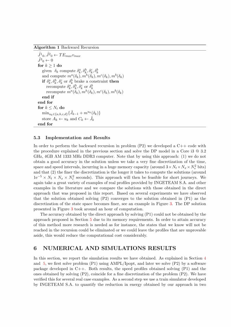
5.3 Implementation and Results

In order to perform the backward recursion in problem (P2) we developed a C++ code withthe procedure explained in the previous section and solve the DP model in a Core i3 @ 3.2GHz, 4GB AM 1333 MHz DDR3 computer. Note that by using this approach: (1) we do notobtain a good accuracy in the solution unless we take a very fine discretization of the time,space and speed intervals, incurring in a huge memory capacity (around 3×Nt×Nx×N2

v bits)and that (2) the finer the discretization is the longer it takes to compute the solutions (around1e−5 × Nt × Nx × N2

v seconds). This approach will then be feasible for short journeys. Weagain take a great variety of examples of real profiles provided by INGETEAM S.A. and otherexamples in the literature and we compare the solutions with those obtained in the directapproach that was proposed in this report. Based on several experiments we have observedthat the solution obtained solving (P2) converges to the solution obtained in (P1) as thediscretization of the state space becomes finer, see an example in Figure 33. The DP solutionpresented in Figure 33 took around an hour of computation.

The accuracy obtained by the direct approach by solving (P1) could not be obtained by theapproach proposed in Section 55 due to its memory requirements. In order to attain accuracyof this method more research is needed as for instance, the states that we know will not bereached in the recursion could be eliminated or we could leave the profiles that are unprovableaside, this would reduce the computational cost considerably.

6 NUMERICAL AND SIMULATIONS RESULTS

In this section, we report the simulation results we have obtained. As explained in Section 44and 55, we first solve problem (P1) using AMPL/Ipopt, and later we solve (P2) by a softwarepackage developed in C++. Both results, the speed profiles obtained solving (P1) and theones obtained by solving (P2), coincide for a fine discretization of the problem (P2). We haveverified this for several real case examples. As a second step we use a train simulator developedby INGETEAM S.A. to quantify the reduction in energy obtained by our approach in two

0 10 20 30 40 50 60 700

2

4

6

8

10

12

14

16

18

20

time (t)

spee

d (m

/s)

Direct approachRP speedDP approachtrack profile

track profile

Figure 3: Comparison of the solution of problem (P1) and (P2).

different rides of a metro in a major city in Europe.The main conclusions regarding the numerical results are the following:

• Our model (due to the additional constraints), (88)-(1111), captures more accurately thedynamics of a train than existing models in the literature.

• The solution of (P1) is always formed by four possible actions which can be summarizedin Table 22.

• The computation time required to solve (P1) for real examples is below 8 seconds, thusour approach represents a realistic solution that can be implemented in real systems.

• The computational time to solve (P2) is

1e−5 ×N1 ×N2 ×N23 s.

For the example presented in Figure 33 the required time for an accurate solution wouldbe 2 days an a half.

• The memory required to save all the optimal strategies is

3×N1 ×N2 ×N23 bits.

• The energy reduction obtained is larger in tracks that present downhill sections.

• In real examples the energy reduction varies between 8% and 25%.

Table 3: Energy reduction compared to real profiles

Section LAAJR energy RP energy Reduction

example 1 15.1485 kWh 16.6101 kWh 8.7995 %

example 2 15.2289 kWh 19.897 kWh 23.4613 %

6.1 Simulations

Simulations carried out in the simulator developed by INGETEAM S.A. allow us to (i) comparethe structure of our profiles with real examples and (ii) to measure the reduction in energy thatour solution would provide. The procedure with the simulator is the following; we provide thespeed profile obtained with Ipopt and the simulator gives the power profile that a train wouldneed to complete the journey determined by this speed and computes the energy consumption.

In Figures 55 and 66 we consider two different real examples from a metro in a major city inEurope. The track in the first example (example 1) presents steep uphill sections in most ofthe track, see Figure 11, and the track in the second example (example 2) presents a flat trackwith a steep downhill section in the end, see Figure 44. We compare the speed and energyconsumptions obtained with the simulations with the profile used in reality and with thatobtained by solving Problem (P1) and (P2).

In Table 33 we represent the energy consumption for the two trips considered. The resultsshow that the solution profile obtained by solving (P1) and (P2) provide a larger reduction inenergy in tracks that present downhill sections, i.e., these tracks are more sensitive, in view ofenergy efficiency, to a good switching strategy. The energy reduction varies between 8% and25% depending on the track considered.

0 10 20 30 40 50 60 70 80 90 1000

5

10

15

time (s)

incl

ine

(m)

Figure 4: Track profile for example 2.

7 CONCLUSIONS AND FUTURE WORK

This paper proposes a robust model for the problem of finding the power and speed profilesthat minimize the energy in short railway journeys. We propose two numerical methods tohandle the difficult constraints that this problem presents avoiding simplifications in the modelas it has been done in the literature.

The efficiency of this methods allow a real application in typical trips of metro systems,being able to: (1) compute new profiles given any circumstance by the approach proposed inSection 44 , and (2) compute off line all the optimal profiles for any possible circumstance bythe approach proposed in Section 55. Our study shows that the method presented in Section 44

0 10 20 30 40 50 60 700

5

10

15

20

25

time

spee

d

RP speed profileLAAJR simulated speed profilemaximum speed

(a) Speed profiles.

0 10 20 30 40 50 60 700

2

4

6

8

10

12

14

16

18

timeen

ergy

LAAR energy consumptionRP energy consumption

(b) Cumulative consumption.

Figure 5: Simulations for example 1.

0 10 20 30 40 50 60 70 80 90 1000

5

10

15

20

25

time

spee

d

RP speed profileLAAJR simulated speed profilemaximum speed

(a) Speed profiles.

0 10 20 30 40 50 60 70 80 90 1000

2

4

6

8

10

12

14

16

18

20

time

ener

gy

LAAR energy consumptionRP energy consumption

(b) Cumulative consumption.

Figure 6: Simulations for example 2.

could be implemented in a real system immediately, whereas more research is required in orderto solve real-life problems with the method of Section 55. Besides, the simulations have shownto obtain a great reduction in the consumption of energy of around 8-25%.

8 ACKNOWLEDGMENTS

The authors gratefully acknowledge the financial support of INGETEAM Traction S.A. duringthe development of this research project and also Albert Gonzalez Manresa (INGETEAMPower Technology - Traction) for the simulations carried out.

References

[1] A. E. Bryson, Jr., Y.C. Ho, Applied Optimal Control: Optimization, Estimation andControl, Hemisphere Wiley, 1975.

[2] A. Grunig, Efficient Generation of Train Speed Profiles, Bachelor’s Thesis, Institute forOperations Research, ETH Zurich, 2009.

[3] A. Wachter, L. T. Biegler, On the Implementation of a Primal-Dual Interior Point FilterLine Search Algorithm for Large-Scale Nonlinear Programming, Mathematical Program-ming, 106(1), pp. 25-57, 2006.

[4] H. Ko, T. Koseki and M. Miyatake, Application of Dynamic Programming to the Op-timization of the Running Profile of a Train, Computers In Railways IX, vol. 15, pp.103-112, 2004.

[5] J. T. Betts, Practical Methods for Optimal Control Using Nonlinear Programming (Ad-vances in Design and Control), Society for Industrial & Applied Mathematics, 2nd editionedition , 2009.

[6] M. Domınguez, A. P. Cucala, A. Fernandez, R.R. Pecharroman, J. Blanquer, EnergyEfficiency on Train Control: Design of Metro ATO Driving and Impact of Energy Accu-mulation Devices, 9th World Congress on Railway Research - WCRR 2011, Lille, France,2011

[7] P.G. Howlett. An optimal strategy for the control of a train Journal of Australian Math-ematical Society Series B, 31 (1990), pp. 454471.

[8] P.G. Howlett, P.J. Pudney, An Optimal Driving Strategy for a Solar Powered Car on anUndulating Road Dynamics of Continuous, Discrete and Impulsive System., 4:553-567,1998.

[9] P. G. Howlett, P. J. Pudney, Energy-efficient Driving Strategies for Long-Haul Trains,Proceedings of CORE 2000 Conference on Railway Engineering, Adelaide, 21-23 May2000.

[10] P. G. Howlett, P. J. Pudney, Energy-efficient Train Control. Springer-Verlag London Ltd.,1995.

[11] R. Fourer, D. M. Gay and B. W. Kernighan, A Modeling Language for MathematicalProgramming. Management Science 36 (1990) 519-554.

[12] W. Zhang, T. Inanc, A Tutorial for Applying DMOC to Solve Optimization ControlProblems, Systems Man and Cybernetics (SMC), 2010 IEEE International Conference,1857 - 1862, Istanbul, 2010.

[13] X. Vu (2006). Analysis of necessary conditions for the optimal control of a train. Ph.D.thesis, University of South Australia (see also www.amazon.co.uk/Analysis-necessary-conditions-optimal-control/dp/3639120000).