Optimize Storage Placement in Sensor Networks

Optimize Storage Placementin Sensor Networks

Bo Sheng, Member, IEEE, Qun Li, Member, IEEE, and Weizhen Mao

Abstract—Data storage has become an important issue in sensor networks as a large amount of collected data need to be archived

for future information retrieval. Storage nodes are introduced in this paper to store the data collected from the sensors in their

proximities. The storage nodes alleviate the heavy load of transmitting all data to a central place for archiving and reduce the

communication cost induced by the network query. The objective of this paper is to address the storage node placement problem

aiming to minimize the total energy cost for gathering data to the storage nodes and replying queries. We examine deterministic

placement of storage nodes and present optimal algorithms based on dynamic programming. Further, we give stochastic analysis for

random deployment and conduct simulation evaluation for both deterministic and random placements of storage nodes.

Index Terms—Wireless sensor networks, data storage, data query.

Ç

1 INTRODUCTION

SENSOR networks deployed for pervasive computingapplications, e.g., sensing environmental conditions

and monitoring people’s behaviors, generate a largeamount of data continuously over a long period of time.This large volume of data has to be stored somewhere forfuture retrieval and data analysis. One of the biggestchallenges in these applications is how to store and searchthe collected data.

The collected data can either be stored in the networksensors or transmitted to the sink. Several problems arisewhen data are stored in sensors. First, a sensor is equippedwith only limited memory or storage space, which prohibitsthe storage of a large amount of data accumulated formonths or years. Second, since sensors are battery operated,the stored data will be lost after the sensors are depleted ofpower. Third, searching for the data of interest in a widelyscattered network field is a hard problem. The communica-tion generated in a network-wide search will be prohibitive.Alternatively, data can be transmitted back to the sink andstored there for future retrieval. This scheme is ideal sincedata are stored in a central place for permanent access.However, the sensor network’s per node communicationcapability (defined as the number of packets a sensor cantransmit to the sink per time unit) is very limited [1], [2]. Alarge amount of data cannot be transmitted from the sensornetwork to the sink efficiently. Furthermore, the datacommunication from the sensors to the sink may take longroutes consuming much energy and depleting of the sensorbattery power quickly. In particular, the sensors around the

sink are generally highly used and exhausted easily, thus,the network may be partitioned rapidly.

It is possible that, with marginal increase in cost, somespecial nodes with much larger permanent storage (e.g.,flash memory) and more battery power can be deployed insensor networks. These nodes back up the data for nearbysensors and reply to the queries. The data accumulated oneach storage node can be transported periodically to a datawarehouse by robots or traversing vehicles using physicalmobility as Data Mule [3]. Since the storage nodes onlycollect data from the sensors in their proximity and the dataare transmitted through physical transportation instead ofhop by hop relay of other sensor nodes, the problem oflimited storage, communication capacity, and batterypower is ameliorated.

Placing storage nodes is related to the sensor networkapplications. We believe that query is the most importantapplication for sensor networks since, in essence, sensornetworks are about providing information of the environ-ment to the end users. A user query may take various forms,e.g., “how many nodes detect vehicle traversing events?”and “what is the average temperature of the sensing field?”In this scenario, each sensor, in addition to sensing thenearby environment, is also involved in routing data for twonetwork services: the raw data transmission to storagenodes and the transmission for query diffusion and queryreply. Two extremes, as mentioned before, would betransmitting all the data to the sink or storing them on eachsensor node locally. On one hand, data solely stored in thesink is beneficial to the query reply incurring no transmis-sion cost, but the data accumulation to the sink is very costly.On the other hand, storing data locally incurs zero cost fordata accumulation, whereas the query cost becomes largebecause a query has to be diffused to the whole network andeach sensor has to respond to the query by transmitting datato the sink. The storage nodes not only provide permanentstorage as described previously but also serve as a bufferbetween the sink and the sensor nodes. The positioning ofstorage nodes, however, is extremely important in this

IEEE TRANSACTIONS ON MOBILE COMPUTING, VOL. 9, NO. 10, OCTOBER 2010 1437

. B. Sheng is with the Department of Computer Science, University ofMassachusetts Boston, 100 Morrissey Boulevard, Boston, MA 02125.E-mail: [email protected].

. Q. Li and W. Mao are with the Department of Computer Science, College ofWilliam and Mary, McGlothlin-Street Hall, Williamsburg, VA 23187-8795. E-mail: {liqun, wm}@cs.wm.edu.

Manuscript received 27 Jan. 2009; revised 15 Aug. 2009; accepted 12 Oct.2009; published online 24 May 2010.For information on obtaining reprints of this article, please send e-mail to:[email protected], and reference IEEECS Log Number TMC-2009-01-0033.Digital Object Identifier no. 10.1109/TMC.2010.98.

1536-1233/10/$26.00 � 2010 IEEE Published by the IEEE CS, CASS, ComSoc, IES, & SPS

communication model. A bad placement strategy may wastethe storage resources and have an adverse effect on theperformance. Therefore, a good algorithm for placingstorage nodes is needed to strike a balance between thesetwo extremes characterizing a trade-off between dataaccumulation and data query.

This paper considers the storage node placementproblem in a sensor network. This problem can be verycomplex with respect to various optimization metrics, suchas bandwidth minimization on each link and lifetime of thenetwork. However, the bandwidth problem is alleviatedbecause the storage nodes collect the data generated withintheir proximities and avoid the heavy load on each linkincurred by the long-distance data communication. Lifetimeof a network depends on the routing scheme and thenetwork structure. Specifically, it is mainly affected by themost loaded nodes, which are likely the nodes close to thesink. The storage placement does not reduce the loads onthose nodes since all the responses have to be sent throughthe nodes around the sink. Therefore, even though lifetimeis an important metric, it is not a good metric to guide thestorage placement design. Instead, we consider an approx-imation of lifetime: energy cost. We believe that energy costis more crucial as it is the most important performancemetric in sensor network design. Therefore, we aim tominimize the total energy cost in data accumulation anddata query by judiciously placing the storage nodes.

We first examine the problem in the fixed tree model. Weassume that the sensor network has organized into a treerooted at the sink. The communication routes from sensorstoward the sink are predefined by the tree. Our goal is toselect some of the nodes in the tree as storage nodes, each ofwhich is responsible for storing the raw data of itsdescendants that are not covered by other storage nodes.In many applications, for example, a sensor network alongthe highway, or a drainage or oil pipeline monitoringsystem, the network communication tree is fixed due to theconstraints of the sensor deployment. Our results for thefixed tree model fit into those scenarios well. We alsoconsider the dynamic tree model, where the (optimal)communication tree is constructed after the storage nodesare deployed. Specifically, each sensor selects a storagenode in its proximity for its data storage with the goal tominimize the energy cost of the resulting communicationtree. The sketch of our solution and preliminary resultshave been published in [4].

The remainder of the paper is organized as follows: InSection 2, we review the related work. In Section 3, wedefine several problems for storage node placement in theaforementioned models. In Sections 4 and 5, we presentoptimal algorithms for the problems defined within thefixed tree model. In Section 6, we give theoretical analysis ofrandomized deployment of storage nodes for both the fixedtree and dynamic tree models. In Section 7, we present oursimulation results, which confirm the theoretical analysis.Finally, in Section 8, we make the conclusion and discussfuture research.

2 RELATED WORK

There have been a lot of prior research works on dataquerying models in sensor networks. In early models [5],

[6], query is spread to every sensor by flooding messages.Sensors return data back to the sink in the reverse directionof query messages. Those methods, however, do notconsider the in-network storage.

In the literature, several schemes have introduced anintermediate tier between the sink and sensors. LEACH [7]is a clustering-based routing protocol, where cluster headscan fuse the data collected from its neighbors to reducecommunication cost to the sink. However, LEACH does notaddress storage problem. Data-centric storage schemes [8],[9], [10], [11], [12], as another category of the related work,store data on different places according to different datatypes. In [8], [9], and [11], the authors propose a data-centricstorage scheme based on Geographic Hash Table, where thehome site of data is obtained by applying a hash function onthe data type. Another practical improvement is proposedin [12] by removing the requirement of point-to-pointrouting. Ahn and Krishnamachari [13] analyze the scalingbehavior of data-centric query for both unstructured andstructured (e.g., GHT) networks and derive some keyscaling conditions. GEM [10] is another approach thatsupports data-centric storage and applies graph embeddingtechnique to map data to sensor nodes. In general, the data-centric storage schemes assume some understanding aboutthe collected data and extra cost is needed to forward datato the corresponding keeper nodes. In our paper, we do notassume any prior knowledge about the data: indeed inmany applications, raw data may not be easily categorizedinto different types. To transmit the collected data to aremote location is also considered expensive because thetotal collected data may be in a very large quantity.

To facilitate data query, Ganesan et al. [14] propose amultiresolution data storage system, DIMENSIONS, wheredata are stored in a degrading lossy model, i.e., fresh dataare stored completely while long-term data are storedlossily. In comparison, our scheme is more general withoutany assumption about the data correlation. PRESTO [15] is arecent research work on storage architecture for sensornetworks. A proxy tier is introduced between sensor nodesand user terminals and proxy nodes can cache previousquery responses. Compared to the storage nodes in thispaper, proxy nodes in PRESTO have no resource constraintsin terms of power, computation, storage, and communica-tion. It is a more general storage architecture that does nottake the characteristics of data generation or query intoconsideration. In the Cougar project [16], [17], a datadissemination tree is built with data sources as leaves. Viewnodes introduced in Cougar have similar functionalities asstorage nodes in this paper. Our scheme focuses more onhow to optimize the placement of storage nodes, whileCougar mainly focuses on how to implement data querywith more details in a sensor network.

In addition, recent research work has shown the feasibilityof storage nodes. Mathur et al. [18] investigate hardwaresupports to attach large-capacity flash memory to sensors.Their measurement study shows that access to large localstorage is practical for sensors. Furthermore, storage nodesare also supported by recent research on software system.Zeinalipour-Yazti et al. propose MicroHash [19], an indexingstructure to manage external flash memory of sensors in

1438 IEEE TRANSACTIONS ON MOBILE COMPUTING, VOL. 9, NO. 10, OCTOBER 2010

order to efficiently look up the stored data. Mathur et al. [20]design Capsule system as an intermediate layer betweenflash memory and sensor applications.

In [21] and [22], the authors introduce an approach toanalyzing communication networks based on stochasticgeometry. They consider models built on Poisson processesand obtain formulas to express the average cost in functionof the intensity parameters of Poisson processes. Baek et al.extend this work specifically to sensor networks in [23]. Ourpaper also analyzes random placement of storage nodes inSection 6. We will use similar means with [21], [22], and [23]to derive analytical formulas for the performance.

3 PROBLEM FORMULATION

In this paper, we consider an application in which sensornetworks provide real-time data services to users. A sensornetwork is given with one special sensor identified as thesink (or base station) and many normal sensors, each ofwhich generates (or collects) data from its environment.Users specify the data they need by submitting queries tothe sink and they are usually interested in the latestreadings generated by the sensors.1 To reply to queries,one typical solution is to let the sink have all the data. Then,any query can be satisfied directly by the sink. This requireseach sensor to send its readings back to the sinkimmediately every time it generates new data. Generally,transferring all raw data could be very costly and is notalways necessary. Alternatively, we allow sensors to holdtheir data and to be aware of the queries, then raw data canbe processed to contain only the readings that users areinterested in and the reduced-size reply, instead of thewhole raw readings, can be transferred back to the sink.This scheme is illustrated in Fig. 1, where the black nodes,called storage nodes, are allowed to hold data. The sinkdiffuses queries to the storage nodes by broadcasting to thesensor network and these storage sensors reply to thequeries by sending the processed data back. Compared tothe previous solution, this approach reduces the raw datatransfer cost (as indicated by the thick arrows in the figures)because some raw data transmissions are replaced by queryreply (as indicated by the thin arrows). On the other hand,this scheme incurs an extra query diffusion cost (asindicated by the dashed arrows). In this paper, we are

interested in strategically designing a data access model tominimize energy cost associated with raw data transfers,query diffusion, and query replies.

We first formally define two types of sensors (or nodes).1) Storage nodes: This type of nodes have much largerstorage capacity than regular sensors. In the data accessmodel, they store all the data received from other nodes orgenerated by themselves. They do not send out anythinguntil queries arrive. Based on the query description, theyobtain the results needed from the raw data they areholding and then return the results back to the sink. Notethat except enriched storage capacity, other resources onstorage nodes are still constrained as regular sensors. Thesink itself is considered as a storage node. 2) Forwardingnodes: This type of nodes are regular sensors and theyalways forward the data received from other nodes orgenerated by themselves along a path toward the sink. Theoutgoing data are kept intact and the forwarding operationcontinues until the data reach a storage node. Theforwarding operation is independent of queries and thereis no data processing at forwarding nodes.

Therefore, our goal is to design a centralized algorithmthat can derive the best locations of the storage nodes to guidethe deployment of such a hybrid sensor network. We makethe following assumptions about the characteristics of datageneration, query diffusion, and query replies: First, for datageneration, we assume that each node generates rd readingsper time unit and the data size of each reading is sd. Second,for query diffusion, we assume that rq queries of the sametype are submitted from users per time unit and the size of thequery messages is sq. Third, for query reply, we assume thatthe size of data needed to reply a query is a fraction�of that ofthe raw data. Specifically, we define a data reductionfunction f for query reply. For input x, which is the size ofraw data generated by a set of nodes, function fðxÞ ¼ �x for� 2 ð0; 1� returns the size of the processed data, which isneeded to reply the query. We do not restrict the types ofqueries we impose on the sensor network in this paper, butwe assume that we can obtain an empirical value for �through examining the historic queries. The parameter �characterizes many queries satisfied by a certain fraction ofall the sensing data, e.g., a range query may be “return all thenodes that sense a temperature higher than 100 degree” and�can be estimated based on the data distribution information.

In this paper, the communication among all n nodes isbased on a tree topology rooted at the sink. The tree is formedin the initial phase as follows: The sink first broadcasts amessage with a hop counter. The nodes receiving the messagewill set the message sender as the parent node, increase thehop counter by 1, and broadcast it. If a node receives multiplemessages, it will select the one with the minimum hopcounter to broadcast and set the sender of the message as itsparent. Data are transferred along the edges in this commu-nication tree. To transmit one data unit, the energy cost of thesender and receiver is etr and ere, respectively, and etr is alsorelevant to the distance between the sender and receiver. Tosimplify the problem, we set the length of each tree edge toone unit, which means that sensor nodes have a fixedtransmission range and the energy cost of transferring data isonly proportional to the data size. Our algorithms can beeasily extended to nonuniform transmission ranges as long as

SHENG ET AL.: OPTIMIZE STORAGE PLACEMENT IN SENSOR NETWORKS 1439

1. Our algorithms also apply to the queries to the historic data. For theease of presentation, we assume that all queries correspond to the latestgenerated data.

Fig. 1. Data access model with storage nodes.

topology information is available. In our energy model, forsimplicity of presentation, the receiving energy cost isassigned to the sender without changing the total energycost. When sensor i sends one data unit to j, the energy cost ofj is 0, and the energy consumed by i is

etr þ ere if j is i0s parent;etr þ ere � ci if j is one of i0s children;

�

where ci is the number of i’s children. In the rest of thispaper, we normalize the energy cost by ðetr þ ereÞ for easypresentation. Thus, transferring one data unit from i to itsparent consumes one energy unit, and to broadcast one dataunit to its children, i will consume bi energy units, wherebi ¼ etrþere�ci

etrþere .Tree structure has been widely used in sensor networks.

Although the communication tree may be broken due to linkfailure, this paper considers a common practice that onlystable links are chosen to build the tree so that errors intransmission due to poor link quality can be reduced and thetree topology can be robust for a long time. Since the treetopology changes will be rare incurring small communica-tion costs compared to the query and data collection cost, wewill not consider the cost for tree topology informationupdate in this paper. If packet loss happens, sensors mayretransmit the packet till it gets through. We assume that theprobability of retransmission is the same for all links. Thus,the energy cost for communication on each link is stillproportional to the data size even though the overhead for aunit packet is larger than that of a perfect wireless link.

The tree structure is independent of the underlying low-layer communication protocol: like myriad routing proto-cols, tree structure is one of the routing schemes. Ouralgorithm only assumes that the energy cost is proportionalto the transmitted data size, which can be realized in manycommunication protocols such as the duty cycle mechan-ism. Moreover, we assume that the applications consideredin this paper can tolerate the delay caused by the low-layercommunication, such as retransmission and duty cyclemechanism. We would also like to mention that the lowerlayer implementation, such as the duty cycle mechanism, iscompatible with the functionality of the tree structure-basedcommunication. Tree structure is constructed in the initi-alization phase in which duty cycle has not been started.Therefore, duty cycle does not affect the tree constructionwhile the tree structure has to be considered for selectingthe parameters for duty cycle.

Here, we present basic analysis of energy cost. Let i be anode in the communication tree and Ti be the subtreerooted at i. We use jTij to denote the number of nodes in Ti.We define eðiÞ to be the energy cost incurred at i per timeunit, which includes the cost for raw data transfer from i toits parent if i is a forwarding node, the cost for querydiffusion if i has storage nodes as its descendants, and thecost for query reply if i is a storage node or has a storagedescendant. To define eðiÞ mathematically, we need toconsider several possible cases.

Case A. i is a forwarding node and there are no storagenodes in Ti. All raw data generated by the nodes in Ti haveto be forwarded to the parent of i and there is no querydiffusion cost. So eðiÞ ¼ jTijrdsd.

Case B. i is a storage node and there are no other storagenodes in Ti. The latest readings of all raw data generated bythe nodes in Ti are processed at node i and the reply size isbe �jTijsd. Node i sends the reply to its parent when queriesarrive. So eðiÞ ¼ rq�jTijsd.

Case C. i is a storage node and there is at least one otherstorage node in Ti. In addition to the cost for query reply asdefined in Case B, i also incurs a cost for query diffusionthat is implemented by broadcasting to its children. SoeðiÞ ¼ rq�jTijsd þ birqsq.

Case D. i is a forwarding node and there is at least onestorage node in Ti. This is the case where all three types ofcost (for raw data transfer, query diffusion, and queryreply) are present. Among the jTij � 1 descendants of i, letd1 be the number of forwarding descendants without anystorage nodes on their paths to i (the raw data generated atthese d1 nodes and at i itself will be forwarded from i to itsparent without reduction) and d2 be the number of storagedescendant’s or forwarding descendants with at least onestorage node on their paths to i (the last readings of the rawdata generated at these d2 nodes would have beenprocessed and reduced before reaching i). Obviously,d1 þ d2 ¼ jTij � 1. So,

eðiÞ ¼ ðd1 þ 1Þrdsd þ birqsq þ rq�d2sd:

The communication tree can be formed before or afterstorage node deployment. Accordingly, we will consider twomodels in the rest of this paper. In the fixed tree model, asillustrated in Fig. 2, we first deploy regular sensors andconstruct a communication tree as usual. Based on thetopology information, we select some of the regular sensorsto be storage nodes. We can attach large flash memory to


Fig. 2. Deploy storage nodes in the fixed tree model (storage nodes are black). (a) Step 1: Regular sensors are deployed in a field. (b) Step 2: Acommunication tree is constructed to relay data. (c) Step 3: Some regular sensors are upgraded to or replaced by storage nodes.

these selected sensors or replace them by more powerfulstorage nodes at the same locations. The other model, thedynamic tree model, is illustrated in Fig. 3. In this model,storage nodes are deployed before the communication tree isformed and their location information is broadcast to nearbyregular sensors. After that, all sensors organize themselvesinto a communication tree according to the locations of thestorage nodes. In both models, after tree construction andstorage node deployment, each storage node needs to send anotification toward the sink. In this way, every sensor isaware of the existence of storage nodes among its descen-dants, and when a query arrives, it is able to determinewhether to continue the diffusion or not.

Within the fixed tree model, we will consider twoproblems of storage node placement. Given an undirectedtree T with nodes labeled as 1; 2; . . . ; n, the length of eachedge is 1. Let eðiÞ be the energy cost of node i in one time unitas defined above. The objective is to place storage sensors(and hence, forwarding sensors) on nodes in T such that thetotal energy cost

Pi2T eðiÞ is minimized. In the case when

there is no limit on the number of storage nodes that can beused to minimize the energy cost, the problem is denoted byUNLIMITED. In the case when there are a limited number ofstorage nodes, say, k, to use, the problem is denoted byLIMITED. For the dynamic tree model, the storage nodeplacement problem becomes how to place k given storagenodes to form a communication tree with the minimum totalenergy cost. This problem is NP-hard since it is a generalcase of the minimum k-median problem. We have proposeda 10-approximation algorithm for the dynamic tree model inour previous work [24].

The above problems defined with the fixed tree anddynamic tree models aim to find the optimal locations forstorage nodes in a deterministic way. In reality, however,the storage nodes may not be deployed in a precise way.Instead, their deployment may be random with a certaindensity �. This paper also evaluates the performance ofrandom deployment of storage nodes in fixed and dynamictrees. Finally, Table 1 lists the notations, which will be usedin the rest of the paper.

4 UNLIMITED NUMBER OF STORAGE NODES

We first present a linear-time algorithm for the problemUNLIMITED, where an unlimited number of storage nodesare available to use to minimize the energy cost of acommunication tree. Recall that eðiÞ is the energy cost at

node i. Let Ti be the subtree rooted at i. Then, EðiÞ is the

energy cost of nodes in Ti, defined to be EðiÞ ¼P

i2Ti eðiÞ.Our algorithm relies on the following lemma:

Lemma 1. Given a node i and its subtree Ti, if �rq � rd, then i

must be a forwarding node to minimize EðiÞ. Otherwise, i

must be a storage node to minimize EðiÞ.Proof. We compare the energy cost of two trees, which are

identical in every aspect except that the first tree’s root is a

forwarding node and the second tree’s root is a storage

node. Let E1 and E2 be the energy cost of these two trees,

respectively. Comparing the energy cost of individual

nodes, one by one, in the two trees, we observe that any two

nonroot nodes in the same position of the trees must have

the same energy cost. The only difference is the energy cost

of the roots. Let e1 and e2 be the energy cost of the roots in

the two trees, respectively. Therefore, E1 � E2 ¼ e1 � e2.

To prove the lemma, it suffices to prove that

e1 � e2� 0 if �rq � rd;> 0 if �rq < rd:

�

We consider two cases. First, if both roots have nostorage descendants, then according to the four-casedefinition of energy cost given in the previous section(Cases A and B, specifically), we have

e1 � e2 ¼ jTijrdsd � rq�jTijsd

¼ jTijsdðrd � �rqÞ� 0 if �rq � rd;> 0 if �rq < rd:

�


Fig. 3. Deploy storage nodes in the dynamic tree model (storage nodes are black). (a) Step 1: Regular sensors and storage nodes are deployed in afield. (b) Step 2: Each storage node (including the sink) broadcasts its location information. (c) Step 3: A communication tree is constructed based onthe locations of storage nodes.

TABLE 1Summary of Notations

Second, if both roots have at least one storage descen-dant, then according to the four-case definition of energycost given in the previous section (Cases D and C,specifically), we have

e1 � e2 ¼ ððd1 þ 1Þrdsd þ birqsq þ rq�d2sdÞ� ðrq�jTijsd þ birqsqÞ

¼ ðd1 þ 1Þsdðrd � �rqÞ� 0 if �rq � rd;> 0 if �rq < rd:

�

In the first tree with a forwarding root, recall that d1 isthe number of forwarding descendants of the rootwithout any storage nodes on their paths to the rootand that d2 is the number of storage descendants plus thenumber of forwarding descendants with at least onestorage node on their paths to the root. Also recall thatd1 þ d2 ¼ jTij � 1. tuFrom the above lemma, we can conclude that if �rq � rd,

then every node (except for the root/sink, which is always astorage node) in the sensor network must be a forwardingnode to minimize the energy cost. However, if �rq < rd,things are a little tricky. Although the root of the tree, say, i,must be a storage node, it may not be true that every node inthe sensor network must be a storage node to minimize theenergy cost. One would think that in order for the tree toincur a minimum energy cost, all of its subtrees should incura minimum energy cost. However, since �rq < rd, theseoptimal subtrees all have storage nodes as their roots. Thismeans that the energy cost of root i will have to include thecost for query diffusion birqsq since it has storage children,i.e., eðiÞ ¼ rq�jTijsd þ birqsq. The cost for query diffusion,however, can be eliminated if all subtrees of i have onlyforwarding nodes, i.e., eðiÞ ¼ rq�jTijsd. (See Cases C and B inthe four-case definition of eðiÞ in the previous section.) Thus,the minimum energy cost of the tree rooted at i should bederived from the better of these two scenarios.

For a tree Ti rooted at i, let Ci be the set of children of i.Let E�ðiÞ be the minimum (optimal) energy cost of Ti. If Ciis empty, i.e., i is a leaf, then i must be a storage node toachieve its minimum energy cost. So E�ðiÞ ¼ rq�sd. If Ci isnot empty, then for any j 2 Ci, let EfðjÞ be the energy costof Tj when all nodes in Tj are forwarding nodes. So

E�ðiÞ ¼ min

(rq�jTijsd þ birqsq þ

Xj2Ci

E�ðjÞ ;

rq�jTijsd þXj2Ci

EfðjÞ):

Algorithm 1 given in pseudocode finds the optimalplacement of storage nodes in two cases: 1) �rq � rd and2) �rq < rd, where the first case is trivial and the second caseis solved by dynamic programming that works from thebottom to the top of the tree. Assume that n nodes in thetree T are labeled using the postorder.2 A table E�½1::n� isused to hold the minimum energy cost of all subtrees rootedat node i ¼ 1; . . . ; n. At the end of the computation, E�½n�

will hold the minimum energy cost of T (which is rooted atn according to the postorder labeling). We also maintain asecond table Ef ½1::n�, which records the energy cost of allsubtrees when all nodes in each subtree are forwardingnodes. In the algorithm, lines 5-9 compute the E� and Ef

entries for all leaves and lines 10-19 compute the E� and Ef

entries for the remaining nodes following our postorder.

Algorithm 1. Place Unlimited Storage Nodes

1: make the root a storage node

2: if �rq � rd then

3: make all nonroot nodes forwarding nodes and return

4: end if

5: for all leaves i do

6: make i a storage node

7: E�½i� ¼ rq�sd8: Ef ½i� ¼ rdsd9: end for

10: for all remaining nodes i, in postorder, do

11: make i a storage node

12: cost1 ¼ rq�jTijsd þ birqsq þP

j2Ci E�½j�

13: cost2 ¼ rq�jTijsd þP

j2Ci Ef ½j�14: E�½i� ¼ minfcost1; cost2g15: Ef ½i� ¼ jTijrdsd þ

Pj2Ci Ef ½j�

16: if cost1 � cost2 then

17: change each descendant of i that is a storage

node to a forwarding node

18: end if

19: end for

There are only OðnÞ entries to compute in tables E� andEf , and to compute each entry that corresponds to a node,only its children will have to be considered. Furthermore,each node starts as a storage node. Once it is changed to aforwarding node by the algorithm, it will never be changedback. Therefore, the time complexity of Algorithm 1 is OðnÞ,where n is the number of nodes.

Summarizing the discussion above, we have the follow-ing theorem:

Theorem 1. If �rq � rd, then the optimal tree with the minimumenergy cost contains only forwarding nodes (except for theroot). If �rq < rd, then the optimal tree can be constructed by adynamic programming algorithm in OðnÞ time.

We also observe that every node starts as a storage nodeand that once it is changed to a forwarding node, all itsdescendants are changed to forwarding nodes as well.Thus, it is impossible for a forwarding node to have astorage descendant. Likewise, it is impossible for a storagenode to have a forwarding ancestor. We then have thefollowing corollary:

Corollary 1. In the optimal tree, if i is a forwarding node, all itsdescendants are forwarding nodes. If i is a storage node, all itsancestors are storage nodes.

In summary, this UNLIMITED problem refers to thescenario that the deployment budget is sufficient toupgrade every sensor to be a storage node. However,simply making all sensors storage nodes may not be thebest strategy. The appropriate deployment still depends on


2. The postorder used in this paper is slightly different from the textbookdefinition of postorder in that our postorder requires all leaves to be listedfirst.

the characteristics of query and data generation. Intuitively,if there are a large volume of queries for a certain set of dataand the reduction function yields a large �, it would bebetter to transfer these data to the sink. On the other hand, ifqueries are infrequent and the reply size is much less thanthe raw data, it would be more efficient to hold the raw datalocally. According to Theorem 1 and Corollary 1, theoptimal deployment of storage nodes has a special prop-erty. For any path from a leave to the root, there is a clearboundary that distinguishes forwarding nodes from storagenodes. The nodes below the boundary layer to leaves areforwarding nodes and the nodes above the boundarytoward the sink are storage nodes.

5 LIMITED NUMBER OF STORAGE NODES

In the problem UNLIMITED discussed in the previoussection, we assume that we have enough storage nodes forthe need to minimize the energy cost of the network. Inreality, however, storage nodes may come with a hardwarecost. Considering a limited budget for deploying a sensornetwork, there might be only a small portion of sensors asstorage nodes. This is why we have also defined the problemLIMITED, which is similar to UNLIMITED except that wehave only k storage nodes to deploy. Since the root (sink) isalways a storage node, we assume that k � 1 and that k� 1is the maximum number of storage nodes that may appearas descendants of the root. Furthermore, from the discussionin the previous section, if �rq � rd, the optimal tree has nostorage nodes at all except the root. In this case, we just donot deploy any of the k� 1 storage nodes and we get anoptimal tree. Our discussion in this section on LIMITED isfor the case of �rq < rd. Since the number of storage nodes islimited, where to place them becomes a crucial problem. Abad placement strategy may hardly improve the perfor-mance. Basically, there is a trade-off between two trends. Onthe one hand, if storage nodes are close to the sink, i.e., at ahigh level in the tree structure, they can process more rawdata, thus reduce the reply size from storage nodes to thesink. However, the sensor network spends much energy intransferring the raw data from low-level forwarding nodesto the storage nodes. On the other hand, if the storage nodesare far away from the sink, the raw data from theirdescendants can be processed earlier along the path towardthe sink. However, storage nodes may cover only a fewregular sensors, which leads to much raw data transferred tothe sink without being processed. Besides this trade-off, thebenefits from a storage node also depend on the locations ofother storage nodes. Therefore, in this section, we proposethe optimal placement strategy in order to maximize thebenefits from deploying k storage nodes.

5.1 Arbitrary Trees

Assume that a communication tree T is given with up tok storage nodes already optimally deployed. By definition,the energy cost of T is

Pi2T eðiÞ. However, we are going to

use a different and unique method to calculate this cost,which works from the bottom of the tree toward the root.Starting from the leaf nodes and following the postorderuntil the root is eventually reached, for each node i, wecompute the energy cost already incurred within the

subtree Ti rooted at i, which is EðiÞ by our notation, plusthe energy cost contributed by the nodes in Ti to theirancestors, which includes both raw data transmission costand query reply cost according to the four-case definition ofthe energy cost of an individual node. Specifically, if i is aforwarding node, it contributes a raw data transmissioncost of rdsd to each of its forwarding ancestors that liebetween i and i’s closest storage ancestor (due to Cases Aand D) and a query reply cost of rq�sd to each of the otherancestors (due to Cases B and D). If i is a storage node,however, it contributes a query reply cost of rq�sd to each ofits ancestors (due to Cases C and D). Fig. 4 depicts the twoscenarios. The top path from node i to the root (sink) iswhen i is a forwarding node and the bottom path from i tothe root is when i is a storage node. Above each node(except i) is the contribution from i to the energy costincurred at the node.

Let l be the number of forwarding nodes between i andits closest storage ancestor, not including i. Let m be theupper bound on the number of storage nodes in Ti. Then,we use Eiðm; lÞ for the energy cost that includes EðiÞ andthe amount contributed by the nodes in Ti to the energy costof their ancestors. Note that 0 � m � k and 0 � l � n� 2. Inthe case that i is a storage node or i’s parent is a storagenode, l becomes 0. Furthermore, if m ¼ 0, no storage node isused in Ti, and if m � 1, at least one but no more thanm storage nodes are used in Ti. Therefore, Enðk; 0Þ is theminimum energy cost of T with up to k storage nodes todeploy, assuming that n is the label for the root.

When traversing the nodes in postorder in the treestarting from the leaves, let i be the current node beingtraversed. Let di be the depth of i in the tree, which is thenumber of edges on the path from i to the root n. We candefine Eiðm; lÞ recursively. For notational simplicity, wefirst define Q0ðmÞ and Q1ðmÞ as follows:

Qi0ðmÞ ¼

0 if m ¼ 0;birqsq if m � 1:

�; Qi

1ðmÞ ¼ Qi0ðm� 1Þ:

If i is a leaf node, Eiðm; lÞ includes the energy cost of iand the precalculated amount contributed by i to all of its diancestors. Specifically, if i is a forwarding node, its ownenergy cost is rdsd and its contribution to the energy cost ofits ancestors is lrdsd þ ðdi � lÞrq�sd. If i is a storage node, itsown energy cost is rq�sd and its contribution to the energycost of its ancestors is dirq�sd. Therefore,

Eiðm; lÞ ¼ðlþ 1Þrdsd þ ðdi � lÞrq�sd if m ¼ 0;

ðdi þ 1Þrq�sd if m � 1:

�

If i is a forwarding nonleaf node with a child set ofCi, the upper bound m must be divided among all of


Fig. 4. Computing the contribution to the energy cost of all ancestors.

its children. Let P ðmÞ be the set of all permutationsp ¼ ðmp

j jj 2 CiÞ, whereP

j2Ci mpj ¼ m and mp

j denotes theupper bound on the number of storage nodes for subtree Tjin permutation p. Then, Eiðm; lÞ is defined to be the sum ofthe amount from all of its subtrees,

min8p2P ðmÞ

Xj2Ci

Ej

�mpj ; lþ 1

�( );

the energy cost of i, rdsd þQi0ðmÞ, and the precalculated

amount of energy cost contributed by i to its ancestors,lrdsd þ ðdi � lÞrq�sd. So,

Eiðm; lÞ ¼ min8p2P ðmÞ

Xj2Ci

Ej

�mpj ; lþ 1

�( )

þ ðlþ 1Þrdsd þ ðdi � lÞrq�sd þQi0ðmÞ:

If i is a storage nonleaf and nonroot node, the upperbound m� 1 must be divided among all of its children. LetP ðm� 1Þ be the set of all permutations p ¼ ðmp

j jj 2 CiÞ,where

Pj2Ci m

pj ¼ m� 1 and mp

j denotes the upper boundon the number of storage nodes for subtree Tj inpermutation p. Then, Eiðm; lÞ is defined to be the sum ofthe amount from all of its subtrees,

min8p2P ðm�1Þ

Xj2Ci

Ejðmpj ; 0

( );

the energy cost of i, rq�sd þQi1ðmÞ, and the precalculated

amount of energy cost contributed by i to its ancestors,dirq�sd. So,

Eiðm; lÞ ¼ min8p2P ðm�1Þ

Xj2Ci

Ej

�mpj ; 0�( )

þ ðdi þ 1Þrq�sd þQi1ðmÞ:

Algorithm 2 given here maintains a two-dimensionalðkþ 1Þ � ðn� 1Þ table, Ei½m; l�, at each node i, where 0 �m � k and 0 � l � n� 2. Assume that a postorder traversalis done beforehand and that the depth of each node iscomputed beforehand. Both the postorder and the depthscan be obtained in OðnÞ time. In the algorithm, lines 1-6compute the Ei tables for all leaves i, lines 7-12 compute theEi tables for the remaining nonroot nodes i, and lines 13and 14 compute the entry En½k; 0� for the root n. After all thetables are constructed, the minimum energy cost of the treewith up to k storage nodes can be found in the entryEn½k; 0�. Note that instead of constructing a table for thestorage root n, we compute only the needed entry for n.

Algorithm 2. Place Limited Storage Nodes

1: for all leaves i do

2: for m ¼ 0 to k do

3: for l ¼ 0 to n� 2 do

4: if m ¼ 0 then

5: Ei½m; l� ¼ ðlþ 1Þrdsd þ ðdi � lÞrq�sd6: if m � 1 then Ei½m; l� ¼ ðdi þ 1Þrq�sd7: for all remaining nonroot nodes i, in postorder, do


9: for l ¼ 0 to n� 2 do

10: min1 ¼ min8p2P ðmÞfP

j2Ci Ej½mpj ; lþ 1�g

þ ðlþ 1Þrdsd þ ðdi � lÞrq�sd þQi0ðmÞ

11: min2 ¼ min8p2P ðm�1ÞfP

j2Ci Ej½mpj ; 0�g

þ ðdi þ 1Þrq�sd þQi1ðmÞ

12: Ej½m; l� ¼ minfmin1;min2g13: En½k; 0� ¼ min8p2P ðk�1Þf

Pj2Cn Ej½mp

j ; 0�gþ rq�sd þQi

1ðmÞ14: return En½k; 0�

Assume that every node in the tree has at most c children.

To partition an upper bound m into up to c upper bounds

with the sum equal to m, there are at most mþc�1m

� �¼

mþc�1c�1

� �� kþc�1

c�1

� �permutations. The algorithm constructs

OðnÞ tables and each table consists of OðknÞ entries. To

compute each entry, the time is

Okþ c� 1

c� 1

� �c

� �¼ Oððkþ c� 1Þc�1c=ðc� 1Þ!Þ

¼ Oððmaxfk; cgÞc�1Þ:

Thus, the time complexity of the algorithm isOðkn2ðmaxfk; cgÞc�1Þ. We summarize the discussion abovein the following theorem:

Theorem 2. Given a communication tree with n nodes and atmost c children for each parent, let k be the maximumnumber of storage nodes that may be deployed in the tree.Then, the optimal tree with the minimum energy cost can beconstructed by a dynamic programming algorithm inOðkn2ðmaxfk; cgÞc�1Þ time.

5.2 Regular Trees

Now we consider a special case of LIMITED, where thegiven network is a regular tree with exactly c children foreach nonleaf node and all leaves at the same level. For sucha c-ary regular tree, we can modify Algorithm 2 to achieve afaster time complexity by making use of the regularity ofthe tree structure.

First, any subtree in a regular tree is also a regular treeand nodes at the same level have the subtrees with the sametopology. This suggests that instead of keeping a table foreach node as in Algorithm 2, we may keep just one table foreach level. We name the levels from bottom to top, with allleaves at level 0, all parents of the leaves at level 1, andfinally, the root at level blogc nc. For each level h, we define atwo-dimensional table Eh½m; l� for 0 � m � k and0 � l � blogc nc � 1, which returns the energy cost incurredwithin the subtree rooted at level h plus the contributionfrom the nodes in the subtree to their ancestors. As usedpreviously, m is still the maximum number of storage nodesto use in the subtree and l is the number of forwardingnodes between the root of the subtree and the storageancestor closest to the root of the subtree.

We first define Q0ðmÞ and Q1ðmÞ as follows:

Q0ðmÞ ¼0 if m ¼ 0;etr þ c � ereetr þ ere

rqsq if m � 1:

(Q1ðmÞ ¼ Q0ðm� 1Þ:

Let H ¼ blogc nc. Algorithm 3 first computes the tableE0½m; l� for all leaves at level 0, for 0 � m � k and 0 � l �H � 1 in lines 2-5. Then it works its way up, level by level,until level H � 1 in lines 6-11. The root, which is at level H,


is treated in lines 12 and 13, differently from the othernodes since it must be a storage node. By using one table foreach level, our algorithm will construct blogc nc tables. Thiswill result in savings in both space and time, comparedwith our algorithm for arbitrary trees, which needs toconstruct n tables. The modified Algorithm 3 for regulartrees has a time complexity of OðkðlognÞ2ðmaxfk; cgÞc�1Þ.

Algorithm 3. c-ary Regular Tree1: H ¼ blogc nc2: for m ¼ 0 to k do

3: for l ¼ 0 to H � 1 do

4: if m ¼ 0 then E0½m; l� ¼ ðlþ 1Þrdsd þ ðH � lÞrq�sd5: if m � 1 then E0½m; l� ¼ ðH þ 1Þrq�sd6: for h ¼ 1 to H � 1 do


8: for l ¼ 0 to H � 1 do

9: min1 ¼ min8p2P ðmÞfPc

j¼1 Eh½mpj ; lþ 1�g

þ ðlþ 1Þrdsd þ ðH � h� lÞrq�sd þQ0ðmÞ10: min2 ¼ min8p2P ðm�1Þf

Pcj¼1 Eh½mp

j ; 0�gþ ðH � hþ 1Þrq�sd þQ1ðmÞ

11: Eh½m; l� ¼ minfmin1;min2g12: EH ½k; 0� ¼ min8p2P ðk�1Þf

Pcj¼1 EH�1½mp

j ; 0�gþ rq�sd þQ1ðmÞ

13: return EH ½k; 0�The result of the algorithm can be summarized in the

following theorem:

Theorem 3. Given a c-ary regular tree with n nodes, let k be themaximum number of storage nodes that may be deployed.Then, the optimal tree with the minimum energy cost canbe constructed by a dynamic programming algorithm inOðkðlognÞ2ðmaxfk; cgÞc�1Þ time.

6 STOCHASTIC ANALYSIS

The algorithms in the previous sections aim to find theoptimal locations for storage nodes. In practice, however,sensors including the storage nodes may not be deployed ina deterministic way. Instead, random deployment ofsensors is commonly seen in applications. In this section,we analyze the performance of random deployment ofstorage nodes in both fixed tree and dynamic tree models.

6.1 Fixed Tree Model

Assume that the forwarding nodes and storage nodes arerandomly distributed to the field with density � and �s,respectively. For simplicity, we consider a disk network field,where the sink is placed at the center and R is the radius. Inthe fixed tree model, the network builds a communicationtree in which each node finds the shortest path to the sink byfollowing the tree edges. Each forwarding node sends its datato the first ancestor storage node on the path to the sink. Asour simulation and other previous research show, the radius(ri) of the area covered by the nodes that are i hops or lessfrom the sink is proportional to i. Let this ratio be c0 ¼ ri

i ,Thus, we can estimate the number of nodes whose distancesto the sink are between ðt� 1Þc0 and tc0, i.e., the nodes withdepth t. Let numðtÞ represent the total number of the nodeswhose depth values are t,

numðtÞ ¼ ��ðt2c02 � ðt� 1Þ2c02Þ ¼ ��ð2t� 1Þc02:

For a node with depth t, let sðtÞ be the expected hop distanceto its closest storage ancestor. The cost caused by this node isrdsd � sðtÞ þ rq�sd � ðt� sðtÞÞ. The probability that an indivi-dual node is a storage node is p ¼ �s

� . Therefore,

sðtÞ ¼ p � 0þ pð1� pÞ � 1þ pð1� pÞ2 � 2þ � � �þ pð1� pÞt�1 � ðt� 1Þ þ ð1� pÞt � t

¼ 1

p� 1

� �ð1� ð1� pÞtÞ:

The total energy cost in this model can be expressed as

E ¼XRc0t¼1

numðtÞðrdsdsðtÞ þ rq�sdðt� sðtÞÞÞ þ Eq;

where Eq is the cost of query diffusion. The value of c0 isrelated to the communication range and node density. Wecan obtain the value from simulation.

Query messages are diffused from the sink to everystorage node. For each storage node, it incurs an extra querydiffusion cost along the path to its closest storage ancestor. Ifwe assume that there is no overlap among the pathsconnecting each storage node and its closest storage ancestor,the total query diffusion cost Eq can be formulated as

Eq ¼XRc0t¼1

num0ðtÞrqsqsðtÞ; ð1Þ

where num0ðtÞ ¼ �s�ð2t� 1Þc02 is the number of storagenodes whose depth values are t and recall that sðtÞ is theexpected distance to the closest storage ancestor.

6.2 Dynamic Tree Model

The fixed tree model assumes that the communication treedoes not change according to the placement of the storagenodes. In the dynamic tree model, after the storage nodeshave been positioned, each sensor node chooses the beststorage node for storage with respect to the minimalcommunication cost for data forwarding and query diffu-sion and reply. The storage node placement in this model ismore complicated than that in the fixed tree model becausewe need to consider the interplay between the storage nodeplacement and the selection of the storage node for eachsensor. These two steps affect each other dynamically.

In the optimal solution, a storage node should send queryreply to the sink by following the shortest path because thedata from a storage node cannot be further reducedaccording to the definition of data reduction function. Aforwarding node has to choose a storage node for datastorage to minimize the total communication cost for its dataincluding raw data transfer to the storage node and queryreply from the storage node to the sink. Therefore, the closeststorage node may not be the best choice if it is further awayfrom the sink yielding more cost on query reply. Assume thatthe sink is located at the origin. Let ~xi represent the location ofsensor i and fdð~xiÞ indicate the location of the forwardingdestination (storage node) assigned to sensor i. If i is a storagenode, then fdð~xiÞ ¼ ~xi. The energy cost of sending raw datafrom ~xi to fdð~xiÞ is rdsdj~xi � fdð~xiÞj. The query reply cost forthe data from forwarding node i is rq�sdjfdð~xiÞj. In total,


the cost generated by a single node i in a time unit isrdsdj~xi � fdð~xiÞj þ rq�sdjfdð~xiÞj. To find the optimal solution,we need to minimize the cost for each sensor.

The total energy cost in this model is

E ¼Xi

ðrdsdj~xi � fdð~xiÞj þ rq�sdjfdð~xiÞjÞ þ Eq; ð2Þ

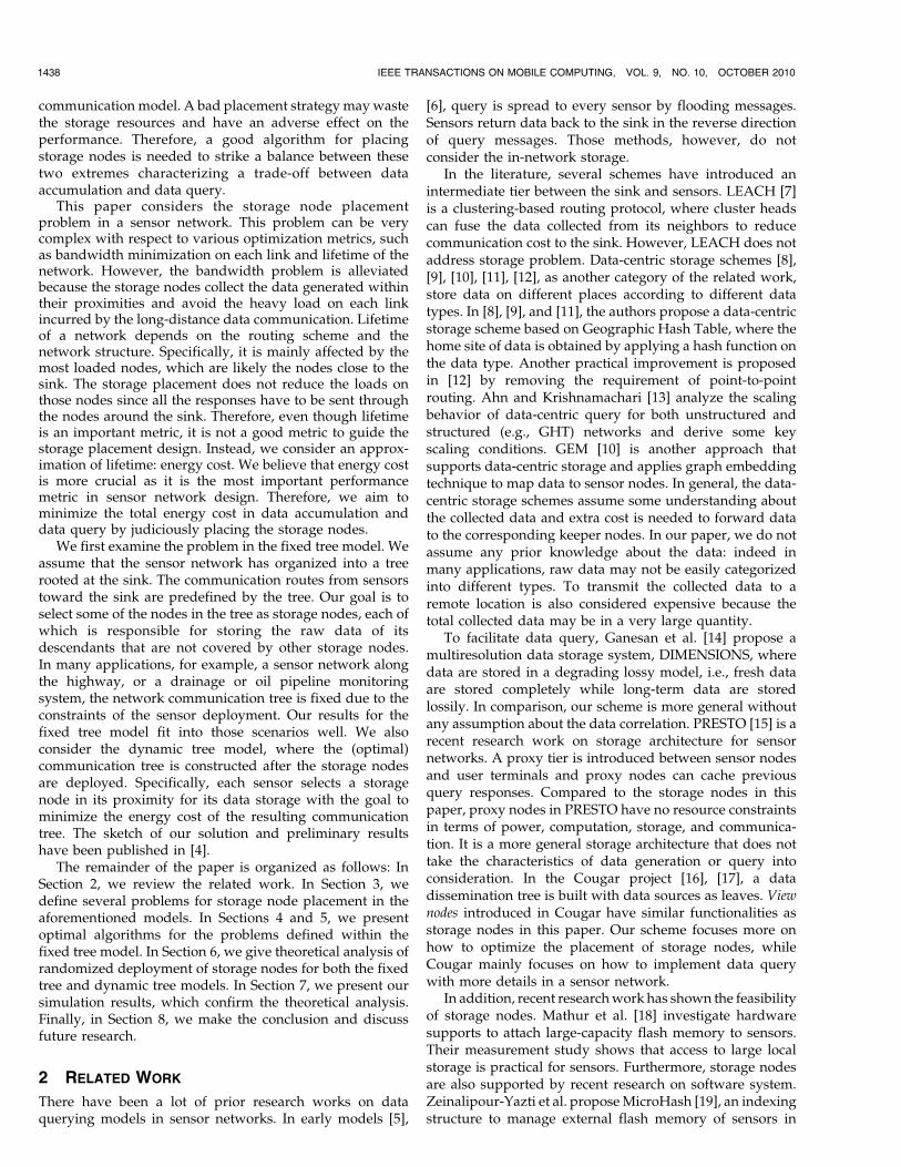
where Eq is the cost of query diffusion. We find that Eq inthis dynamic tree model is the same as that in the fixed treemodel. Because in both models, each storage node isconnected to the sink by the shortest path. Therefore, wecan also use (1) to estimate Eq. In the following of thissection, we will analyze the rest part of (2), which isdenoted by E0.

First, let us consider a scenario where a sensor atlocation ~x forwards its raw data to a storage node atlocation ~y. We define a function F ð~x;~yÞ as the energy costcaused by this sensor, F ð~x;~yÞ ¼ rdsdj~x�~yj þ rq�sdj~yj. Thereare requirements for this scenario to be valid. Essentially,for the sensor at ~x, no other storage node could yield lesscost than the one at ~y. Next, we will derive this condition.We define an area Gð~x;UÞ ¼ f~yjF ð~x;~yÞ � Ug, that is, if asensor at ~x selects any storage node in that area, the energycost for the data of that sensor would be no more than U .Thus, Gð~x; F ð~x;~yÞÞ \ S ¼ � is the requirement for the abovescenario. Considering the Poisson deployment of sensors,the minimum reply cost can be expressed as

E0 ¼ �ZZ

P ð~y 2 SÞF ð~x;~yÞP ðGð~x; F ð~x;~yÞÞ \ S ¼ �Þdydx;

where S is the set of all storage nodes including the sink.P ð~y 2 SÞ is the probability that there is a storage node atlocation ~y,

P ð~y 2 SÞ ¼ 1 if ~y is the origin;�s; otherwise:

�

P ðGð~x; F ð~x;~yÞÞ \ S ¼ �Þ represents the probability ofGð~x; F ð~x;~yÞÞ \ S ¼ �. As we described before, this condi-tion means that there is no other storage node in the areaGð~x; F ð~x;~yÞÞ. According to the Poisson process of deployingstorage nodes with the density �s,

P ðGð~x;F ð~x;~yÞÞ \ S ¼ �Þ

¼ e��sjGð~x;F ð~x;~yÞÞj if F ð~x;~yÞ � F ð~x; 0Þ;0; otherwise:

(

Unlike other nodes, the sink is deterministically fixed in thenetwork. So if area G covers the sink, there is no need tocompute the probability. The forwarding node will defi-nitely send data directly to the sink.

However, jGj in the formula above, called the CartesianOval, cannot be expressed in a closed form. To approximatethe energy cost, we make each forwarding node simplychoose the closest storage node for data storage. Thenetwork field is then divided into Voronoi cells inducedby storage nodes. The energy cost of this topology is veryclose to the optimal case, especially when �s �.

Assume that there is a forwarding node i at location ~x,the probability that i sends data through a storage node atlocation ~y becomes

P ð~x! ~yÞ ¼0 if j~x�~yj � j~xj;e��s�j~xj

2

if ~y is the origin;

�se��s�j~x�~yj2; otherwise:

8<:

Thus,

E0 ¼ �ZZ

F ð~x;~yÞP ð~x! ~yÞdydx

¼ �ZF ð~x; 0Þe��s�j~xj

2

dx

þ �ZZj~x�~yj<j~xj

F ð~x;~yÞ�se��s�j~x�~yj2

dydx:

ð3Þ

In the first term, F ð~x; 0Þ ¼ rdsdj~xj. Therefore,

�

ZF ð~x; 0Þe��s�j~xj

2

dx ¼ �rdsdZj~xje��s�j~xj

2

dx

¼ 2��rdsd

Z R

0

�2e��s��2

d�:

ð4Þ

For the second term in (3), Fig. 5 shows the variables aftercoordination conversions, where � ¼ j~x�~yj and �0 ¼ j~xj.F ð~x;~yÞ can be expressed by rdsd�þ rq�sd

ffiffiffiffiffiffiffiffiffiffiffiffiffiffiffiffiffiffiffiffiffiffiffiffiffiffiffiffiffiffiffiffiffiffiffiffiffi�02þ�2�2 cos ��0�

p.

Thus, the second term becomes

�

ZZj~x�~yj<j~xj

F ð~x;~yÞ�se��s�j~x�~yj2

dydx

¼ 4�2��srdsd

Z R

0

Z �0

0

e��s��2

�2�0d�d�0

þ 2��srq�sd

Z R

0

Z 2�

0

Z �0

0

e��s��2

��0ffiffiffiffiffiffiffiffiffiffiffiffiffiffiffiffiffiffiffiffiffiffiffiffiffiffiffiffiffiffiffiffiffiffiffiffiffiffiffiffiffi�02 þ �2 � 2 cos ��0�

qd�d�d�0:

ð5Þ

Combining (4) and (5), the total energy cost except querydiffusion is

E0 ¼ 2��rdsd

Z R

0

�2e��s��2

d�

þ 4�2��srdsd

Z R

0

Z �0

0

e��s��2

�2�0d�d�0

þ 2��srq�sd

Z R

0

Z 2�

0

Z �0

0

e��s��2

��0ffiffiffiffiffiffiffiffiffiffiffiffiffiffiffiffiffiffiffiffiffiffiffiffiffiffiffiffiffiffiffiffiffiffiffiffiffiffiffiffiffi�02 þ �2 � 2 cos ��0�

qd�d�d�0:

We can further approximate E0 by examining its twocomponents separately. Let Efs be the cost of transferringraw data between forwarding nodes and their closeststorage nodes. Let Ess be the cost to relay reply fromstorage nodes to the sink. For a forwarding node i, theexpected distance to the closest storage node is 1

2ffiffiffiffi�sp . Thus,


Fig. 5. A forwarding node at location~x sends data via a storage node at~y.

Efs ¼ ��R2rdsd1

2ffiffiffiffiffi�sp ; ð6Þ

where ��R2 is the total number of forwarding nodes and

rdsd1

2ffiffiffiffi�sp is the energy cost of transferring raw data from an

individual forwarding node to its closest storage node. In

addition, Ess ¼ rq�sdP

i2SðDi þ 1ÞLi, where Di is the total

number of descendants and Li is the distance to the sink.

Since each forwarding node chooses the closest storage

node for data storage, the number of forwarding nodes that

each storage node is responsible for is approximately the

same. If we replace Li by the mean value L0, then

Ess ¼ rq�sdL0P

i2SðDi þ 1Þ, whereP

i2SðDi þ 1Þ represents

the number of nodes that send data via storage nodes to the

sink. Let N 0 be the number of forwarding nodes that send

data directly to the sink,P

i2SðDi þ 1Þ ¼ ��R2 �N 0. N 0 can

be derived as

N 0 ¼ �Ze��s�j~xj

2

dx ¼ �Z 2�

0

Z R

0

e��s��2

�d�d�

¼ 2��

Z R

0

�e��s��2

d� ¼ �

�sð1� e��s�R2Þ:

And L0 can be simply approximated as

L0 ¼�sRR

0 2�r � rdr�s�R2

¼ 2

3R:

Therefore,

Ess ¼ rq�sd2

3R ��R2 � �

�sð1� e��s�R2Þ

� �� : ð7Þ

Combining (6) and (7),

E0 ¼ ��R2rdsd1

2ffiffiffiffiffi�sp

þ rq�sd2

3R ��R2 � �

�sð1� e��s�R2Þ

� �� :

7 PERFORMANCE EVALUATION

Our evaluation is based on simulation. In this section, we will

present the performance results of the proposed algorithms.

7.1 Simulation Settings

In our simulation, we consider a network of sensors deployed

on a disk of radius 5 with the sink placed at the center. One

thousand sensor nodes (n ¼ 1;000) are deployed to the field

randomly following two-dimensional spatial Poisson pro-

cess. Node transmission range is set to 0.65. After all nodes

are deployed, a routing tree rooted at the sink is constructed

by flooding a message from the sink to all the nodes in the

network. As we mentioned in Section 3, the message carries

the number of hops it travels so that each node chooses

among its neighbors the node that has the minimum number

of hops to be its parent. This tree topology is needed in the

simulation of the fixed tree model. This step, however, can be

skipped for the dynamic tree model.In the rest of this section, we will present and compare

the following algorithms:

. FT-DD: It represents the fixed tree model withdeterministic deployment. In FT-DD, the storagenodes are deployed by following the dynamicprogramming algorithm according to the knowntree topology.

. FT-RD: It represents the fixed tree model withrandom deployment. In FT-RD, we randomly selecta certain number of nodes in the network to bestorage nodes.

. DT-RD: It represents the dynamic tree model withrandom deployment. In this algorithm, the storagenodes are randomly deployed. After that, eachforwarding node selects the best storage node todeliver data and each storage node replies to queryby following the shortest path to the sink.

. ST-RD: It represents semidynamic tree model withrandom deployment, which is the enhanced versionof FT-RD with a local adjustment. When a sensor i isupgraded to storage node in a tree structure, itssiblings’ children will try to set i as their parents if iis within their communication range.

. Greedy: It represents a greedy algorithm where themost heavily loaded sensors will be upgraded tostorage nodes. Usually, those sensors close to thesink will become storage nodes in this algorithm.

This list does not include the existing in-network storageapproaches such as data-centric storage because the problemsettings are different for a comparison. Approximately, theperformance of data-centric storage is close to the randomdeployment in dynamic tree model in this paper since thelocations of storage sites are determined by hash values.

In addition, we use relative energy cost as performancemetrics. We measure the cost when no storage node exceptthe sink is deployed as the baseline. Let the energy cost in thisno storage scenario be Ef . And let the energy cost after thestorage nodes are deployed be E. The relative energy cost isdefined as E

Ef, represented as a percentage. In the rest of this

section, we use “energy cost” for “relative energy cost.”Due to the randomness of our simulation environment,

results from the same parameter setting might vary a lot.Therefore, for a certain set of parameters, we conduct 100independent trials and the average energy cost is used inthe following analysis and comparison. Unless otherwisestated, we set the following parameters in our simulations:rd ¼ rq ¼ sd ¼ sq ¼ 1 and � ¼ 0:5. We evaluate the energycost by varying the number of storage nodes k and the datareduction rate �. Note that the energy cost is also related tord; sd; rq, and sq. However, for comparison purpose,changing rq; sq; rd; sd will be equivalent to changing �. Tosimplify the description, we fix rq; sq; rd; sd and only vary �to examine different characteristics of data and queries.

7.2 Random Deployment

Fig. 6 shows the energy cost of random deployment in thefixed tree model. We compare our theoretical estimationwith simulation results. As we can see from the figure, thetheoretical estimation and the simulation match well. Wehave examined the simulation carefully and found thatmany storage nodes are placed at the leaf nodes or have veryfew descendants. Therefore, the data reduction for thosedescendants is negligible and less energy is saved comparedto the case that each node sends all the data to the sink.


In Fig. 7, we show the energy cost with respect todifferent data reduction rates �. We fix the number ofstorage nodes (k ¼ 10) and change the data reduction rate �from 0.1 to 0.9. In this fixed tree model, decreasing datareduction rate cannot improve the performance too much.Even when � is set to 0.1, we still have more than 96 percent

energy cost with 10 storage nodes. The reason is that dataaccumulation to the storage nodes from the forwardingnodes consumes most of the energy with respect to thequery diffusion and reply. Moreover, when � is 0.9, theenergy cost is even worse than the original cost because theincurred query diffusion cost becomes larger than thebenefits obtained.

The energy cost of random deployment in the dynamictree model is shown in Fig. 8. In this model, the location ofeach storage node is broadcast to forwarding nodes so thatthey can choose the proper storage nodes to deliver data forthe energy concern. In this way, we take full advantage of

every storage node and maximize their contributions to thewhole network. As shown in Fig. 8, random deploymentperforms much better in this dynamic tree model. Theenergy cost decreases very fast with increasing number ofstorage nodes, e.g., with 10 storage nodes (1 percent of totalnodes), we can save energy by approximately 20 percent.

Fig. 9 illustrates the impact of data reduction rate to theenergy cost in the dynamic tree model. This time, �becomes an important parameter because every storagenode is in charge of many forwarding nodes in the dynamictree model. A small decrease of � will reduce energy costgreatly. We also observe that our theoretical estimationmatches well with the simulation results. Although ourstochastic analysis uses some expected values and approx-imations, the maximum difference between the two curvesis less than 5 percent.

As shown above, with random deployment, the dynamictree model has a significant performance improvement overthe fixed tree model. However, the locations of storage nodesneed to be broadcast to all other nodes and the new tree iscompletely different from the originally constructed tree one.We consider a semidynamic tree model in which localadjustments are applied to the originally constructed tree.For each storage node i, all the forwarding nodes within thetransmission range of i that have a depth no less than i’sdepth select i as parent. As a result, each storage node gainsmore descendants and accepts more raw data storage. Fig. 10compares the energy cost of random deployment in threemodels (fixed tree, dynamic tree, and semidynamic tree), aswell as deterministic deployment in the fixed tree model. Asshown in Fig. 10, DT-RD achieves the best performance,while FT-RD has the worst performance. Local adjustment inST-RD improves the performance of the fixed tree model. InFT-RD, each storage node has no control about how manydescendants it can have. Many storage nodes are deployedwith few descendants, which explains why FT-RD deliversthe worst performance. ST-RD allows each storage node tohave some restrained flexibility in choosing its descendants,and has a better performance than FT-RD. DT-RD has moreflexibility in choosing descendants, and we see a muchimproved performance.


Fig. 6. FT-RD: Energy cost with varying number of storage nodes ðkÞ.

Fig. 7. FT-RD: Tthe impact of data reduction rate ð�Þ.

Fig. 8. DT-RD: Energy cost with varying number of storage nodes ðkÞ.

Fig. 9. DT-RD: The impact of data reduction rate ð�Þ.

Fig. 10. Comparison of energy cost with varying number of storage

nodes ðkÞ.

7.3 Deterministic Deployment

Figs. 11 and 12 illustrate the performance of deterministicdeployment in the fixed tree model. In the simulation, thelocations of the storage nodes are obtained by Algorithm 2.Compared to the random deployment (FT-RD) and greedyalgorithm, deterministic deployment significantly improvesthe performance by precisely computing the optimalpositions to put the storage nodes.

In Fig. 11, we fix the reduction rate � ¼ 0:5, and vary thenumber of storage nodes from 2 to 25. With a few storagenodes, the energy cost is sharply reduced in Fig. 11. When kbecomes larger, the slope gradually becomes flatter. Asshown in the figure, we can save about 20 percent energycost with 10 storage nodes, and 30 percent with 25 storagenodes. In addition, Fig. 12 shows the energy cost withvarying reduction rate, when the number of storage nodesis fixed as 10. As we can see, the energy cost is nearly linearto the reduction rate �.

Intuitively, the performance in the fixed tree modeldepends on which level of the tree the storage nodes aredeployed at. When storage nodes are close the leaves, whichoften happens in FT-RD, the benefit of data reduction islimited. On the other hand, when storage nodes are deployedclose to the sink as in the greedy algorithm, a large amount ofraw data have to traverse a long path to reach the storagenodes still yielding high energy cost. The locations derivedfrom our algorithm usually reside in the middle levels. Hereis an example of the result. Table 2 shows the depthdistribution in a particular tree structure. The depth of the

sink is 0. When we deploy 10 storage nodes in such a tree, thederived depths of storage nodes are 3, 4, 4, 4, 4, 5, 5, 6, 6, and 6.

7.4 Network Life

Finally, load distribution and network lifetime are shown inFigs. 13 and 14. We show the workloads of the most heavilyloaded 50 nodes in Fig. 13. In Fig. 14, we define lifetime as thetime that 2 percent nodes are depleted of energy. In oursetting, it means that 20 sensors are out of operation.According to our simulation, this scenario will usually causedisconnection in the sensor network. As we can see in Fig. 13,FT-RD almost has no improvement on load balancing andlifetime. In contrast, FT-DD lengthens the lifetime a lot with asmall number of storage nodes, although the objective of ouralgorithm is to minimize the total energy cost. For example,with 15 storage nodes, the lifetime is increased by more than60 percent. DT-RD does not perform well with only a fewstorage nodes because the sensors connecting storage nodesand the sink carry a lot of workloads for both raw datatransmission and reply collection. The greedy algorithm issuperior to DT-RD by specifically reducing the energy cost ofthe most heavily loaded nodes.

8 CONCLUSION

This paper considers the storage node placement problem ina sensor network. Introducing storage nodes into the sensornetwork alleviates the communication burden of sending allthe raw data to a central place for data archiving andfacilitates the data collection by transporting data from alimited number of storage nodes. In this paper, we examinehow to place storage nodes to save energy for data collectionand data query. We consider two models: fixed tree modeland dynamic tree model. In the first model, we give exactsolution on how to place storage nodes to minimize totalenergy cost. Using stochastic analysis, we also give the


Fig. 11. Comparison of FT-DD, FT-RD, and Greedy: Energy cost with

varying number of storage nodes ðkÞ.

Fig. 12. Comparison of FT-DD, FT-RD, and Greedy: The impact of data

reduction rate ð�Þ.

TABLE 2Depth Distribution (D: Depth, #: Number of Sensors)

Fig. 13. Comparison of load balancing: Workload is measured as the

size of the messages sent by each sensor per unit time.

Fig. 14. Comparison of lifetime with varying number of storage nodes

ðkÞ: values are normalized by the lifetime without storage nodes.

performance estimation for both models under the assump-

tion that the storage nodes are deployed randomly.

ACKNOWLEDGMENTS

This project was supported in part by US National Science

Foundation grant nos. CNS-0721443, CNS-0831904, and

CAREER Award CNS-0747108.

REFERENCES

[1] P. Gupta and P.R. Kumar, “The Capacity of Wireless Networks,”IEEE Trans. Information Theory, vol. 46, no. 2, pp. 388-404, Mar.2000.

[2] E.J. Duarte-Melo and M. Liu, “Data-Gathering Wireless SensorNetworks: Organization and Capacity,” Computer Networks(COMNET), vol. 43, no. 4, pp. 519-537, Nov. 2003.

[3] R.C. Shah, S. Roy, S. Jain, and W. Brunette, “Data MULEs:Modeling a Three-Tier Architecture for Sparse Sensor Networks,”Proc. First IEEE Int’l Workshop Sensor Network Protocols andApplications (SPNA), May 2003.

[4] B. Sheng, Q. Li, and W. Mao, “Data Storage Placement in SensorNetworks,” Proc. ACM MobiHoc, pp. 344-355, 2006.

[5] S. Madden, M.J. Franklin, J.M. Hellerstein, and W. Hong, “TAG: ATiny Aggregation Service for Ad-Hoc Sensor Networks,” SIGOPSOpererating Systems Rev., vol. 36, no. SI pp. 131-146, 2002.

[6] S. Madden, M.J. Franklin, J.M. Hellerstein, and W. Hong, “TheDesign of an Acquisitional Query Processor for Sensor Networks,”Proc. ACM SIGMOD, pp. 491-502, 2003.

[7] W. Heinzelman, A. Chandrakasan, and H. Balakrishnan, “Energy-Efficient Communication Protocols for Wireless MicrosensorNetworks,” Proc. Int’l Conf. System Sciences, Jan. 2000.

[8] S. Shenker, S. Ratnasamy, B. Karp, R. Govindan, and D. Estrin,“Data-Centric Storage in Sensornets,” SIGCOMM Computer Comm.Rev., vol. 33, no. 1, pp. 137-142, 2003.

[9] S. Ratnasamy, B. Karp, S. Shenker, D. Estrin, R. Govindan, L. Yin,and F. Yu, “Data-Centric Storage in Sensornets with GHT, aGeographic Hash Table,” Mobile Networks and Applications, vol. 8,no. 4, pp. 427-442, 2003.

[10] J. Newsome and D. Song, “GEM: Graph Embedding for Routingand Data-Centric Storage in Sensor Networks without GeographicInformation,” Proc. First Int’l Conf. Embedded Networked SensorSystems, pp. 76-88, 2003.

[11] Y.-J. Kim, R. Govindan, B. Karp, and S. Shenker, “GeographicRouting Made Practical,” Proc. Second USENIX Symp. NetworkedSystems Design and Implementation (NSDI ’05), May 2005.

[12] C.T. Ee, S. Ratnasamy, and S. Shenker, “Practical Data-CentricStorage,” Proc. Third USENIX Symp. Networked Systems Design andImplementation (NSDI ’06), May 2006.

[13] J. Ahn and B. Krishnamachari, “Fundamental Scaling Laws forEnergy-Efficient Storage and Querying in Wireless Sensor Net-works,” Proc. Seventh ACM Int’l Symp. Mobile Ad Hoc Networkingand Computing, pp. 334-343, 2006.

[14] D. Ganesan, B. Greenstein, D. Estrin, J. Heidemann, and R.Govindan, “Multiresolution Storage and Search in Sensor Net-works,” ACM Trans. Storage, vol. 1, no. 3, pp. 277-315, 2005.

[15] M. Li, D. Ganesan, and P. Shenoy, “PRESTO: Feedback-DrivenData Management in Sensor Networks,” Proc. Third USENIX Symp.Networked Systems Design and Implementation (NSDI ’06), May 2006.

[16] A. Demers, J. Gehrke, R. Rajaraman, N. Trigoni, and Y. Yao, “TheCougar Project: A Work-in-Progress Report,” SIGMOD Record,vol. 32, no. 4, pp. 53-59, 2003.

[17] J. Gehrke and S. Madden, “Query Processing in Sensor Networks,”IEEE Pervasive Computing, vol. 3, no. 1, pp. 46-55, Jan. 2004.

[18] G. Mathur, P. Desnoyers, D. Ganesan, and P. Shenoy, “Ultra-LowPower Data Storage for Sensor Networks,” Proc. Fifth Int’l Conf.Information Processing in Sensor Networks, pp. 374-381, 2006.

[19] D. Zeinalipour-Yazti, S. Lin, V. Kalogeraki, D. Gunopulos, andW.A. Najjar, “MicroHash: An Efficient Index Structure for Flash-Based Sensor Devices,” Proc. Fourth USENIX Conf. File and StorageTechnologies, 2005.

[20] G. Mathur, P. Desnoyers, D. Ganesan, and P. Shenoy, “CAPSULE:An Energy-Optimized Object Storage System for Memory-Con-strained Sensor Devices,” Proc. Fourth Int’l Conf. EmbeddedNetworked Sensor Systems, 2006.

[21] F. Baccelli, M. Klein, M. Lebourges, and S. Zuyev, “StochasticGeometry and Architecture of Communication Networks,”J. Telecomm. Systems, vol. 7, pp. 209-227, 1997.

[22] F. Baccelli and S. Zuyev, “Poisson-Voronoi Spanning Trees withApplications to the Optimization of Communication Networks,”Operations Research, vol. 47, no. 4, pp. 619-631, 1999.

[23] S.J. Baek, G. de Veciana, and X. Su, “Minimizing EnergyConsumption in Large-Scale Sensor Networks through Distrib-uted Data Compression and Hierarchical Aggregation,” IEEE J.Selected Areas Comm., special issue on fundamental performancelimits of wireless sensor networks, vol. 22, no. 6, pp. 1130-1140,Aug. 2004.

[24] B. Sheng, C.C. Tan, Q. Li, and W. Mao, “An ApproximationAlgorithm for Data Storage Placement in Sensor Networks,” Proc.Second Int’l Conf. Wireless Algorithms, Systems and Applications(WASA ’07), Aug. 2007.

Bo Sheng received the PhD degree in computerscience from the College of William and Mary in2010. He is an assistant professor in theDepartment of Computer Science at the Uni-versity of Massachusetts Boston. His researchinterests include wireless networks and em-bedded systems with an emphasis on theefficiency and security issues. He is a memberof the IEEE.

Qun Li received the PhD degree in computerscience from Dartmouth College. He is anassociate professor in the Department of Com-puter Science at the College of William andMary. His research interests include wirelessnetworks, sensor networks, RFID, and pervasivecomputing systems. He received the US Na-tional Science Foundation CAREER Award in2008. He is a member of the IEEE.

Weizhen Mao received the PhD degree incomputer science from Princeton Universityunder the supervision of Andrew C.-C. Yao. Sheis currently an associate professor in the Depart-ment of Computer Science at the College ofWilliam and Mary. Her current research interestsinclude the design and analysis of online andapproximation algorithms for problems arisingfrom application areas, such as multicore jobscheduling and wireless and sensor networks.

. For more information on this or any other computing topic,please visit our Digital Library at www.computer.org/publications/dlib.


Documents

Optimize Storage Placement in Sensor Networks