Optimized Code Generation for Deep Learning Networks using

Optimized Code Generation for

Deep Learning Networks using

LATTE and SWIRL

Janaan LakeUniversity of Utah

UUCS-20-003

School of ComputingUniversity of Utah

Salt Lake City, UT 84112 USA

22 April 2020

Abstract

As Deep Neural Networks (DNNs) become more widely used in a variety of ap-plications, the need for performance and portability on a number of different architec-tures, including CPUs, becomes increasingly important. Traditionally, many DNNframeworks resort to statically-tuned libraries to get performance on specific plat-forms. This approach is limited by the library performance which can vary greatlyacross different data sizes and layouts, memory hierarchies and hardware features.Compiler-based methods are getting increased attention because they offer opportuni-ties for performance gains by exploiting data reuse and parallelism, efficient memoryaccess, and vectorization for specific backends with the use of abstraction.

Training DNNs can be challenging, and the Batch Normalization (BN) operator hasbecome a popular technique for accelerating training and making networks more ro-bust. Most DNN frameworks include an optimized implementation of this operator,but the computation efficiency decreases dramatically when this operator does not fitthe preoptimized version of library functions.

LATTE is a domain-specific language for DNNs, and SWIRL is a compiler that can

1

be used with LATTE. This thesis extends the applicability of LATTE/SWIRL by in-corporating the BN operator into the LATTE framework and by expanding the opti-mizations of SWIRL to apply to this operator. Several common compiler techniques,such as scalar replacement, loop interchange, fusion and unrolling, vectorization andparallelization can be applied to this operator for performance enhancements. Theoptimized BN operator in LATTE/SWIRL is compared to existing frameworks such asTensorFlow, TensorFlow with Intel MKL-DNN, TensorFlow with XLA, PyTorch withMKL-DNN and MXNet with MKL-DNN. The results show that a compiler-based ap-proach for the BN operator can increase performance on CPU architectures.

2

OPTIMIZED CODE GENERATION FOR DEEP

LEARNING NETWORKS USING LATTE AND SWIRL

by

Janaan Lake

A senior thesis submitted to the faculty ofThe University of Utah

in partial fulfillment of the requirements for the degree

Bachelor of Computer Science

School of Computing

The University of Utah

May 2020

Approved:

Mary Hall, PhDThesis Faculty Supervisor

Ross Whitaker, PhDDirectorSchool of Computing

H. James de St. Germain, PhDDirector of Undergraduate StudiesSchool of Computing

mhall

Stamp

ABSTRACT

As Deep Neural Networks (DNNs) become more widely used in a variety of ap-

plications, the need for performance and portability on a number of different ar-

chitectures, including CPUs, becomes increasingly important. Traditionally, many

DNN frameworks resort to statically-tuned libraries to get performance on specific

platforms. This approach is limited by the library performance which can vary

greatly across different data sizes and layouts, memory hierarchies and hardware

features. Compiler-based methods are getting increased attention because they offer

opportunities for performance gains by exploiting data reuse and parallelism, efficient

memory access, and vectorization for specific backends with the use of abstraction.

Training DNNs can be challenging, and the Batch Normalization (BN) operator

has become a popular technique for accelerating training and making networks more

robust. Most DNN frameworks include an optimized implementation of this operator,

but the computation efficiency decreases dramatically when this operator does not fit

the preoptimized version of library functions.

LATTE is a domain-specific language for DNNs, and SWIRL is a compiler that can

be used with LATTE. This thesis extends the applicability of LATTE/SWIRL by

incorporating the BN operator into the LATTE framework and by expanding the op-

timizations of SWIRL to apply to this operator. Several common compiler techniques,

such as scalar replacement, loop interchange, fusion and unrolling, vectorization and

parallelization can be applied to this operator for performance enhancements. The

optimized BN operator in LATTE/SWIRL is compared to existing frameworks such

as TensorFlow, TensorFlow with Intel MKL-DNN, TensorFlow with XLA, PyTorch

with MKL-DNN and MXNet with MKL-DNN. The results show that a compiler-based

approach for the BN operator can increase performance on CPU architectures.

CONTENTS

ABSTRACT . . . . . . . . . . . . . . . . . . . . . . . . . . . . . . . . . . . . . . . . . . . . . . . . . . ii

LIST OF FIGURES . . . . . . . . . . . . . . . . . . . . . . . . . . . . . . . . . . . . . . . . . . . . iv

CHAPTERS

1. INTRODUCTION . . . . . . . . . . . . . . . . . . . . . . . . . . . . . . . . . . . . . . . . . 1

2. BACKGROUND . . . . . . . . . . . . . . . . . . . . . . . . . . . . . . . . . . . . . . . . . . . 5

2.1 Batch Normalization . . . . . . . . . . . . . . . . . . . . . . . . . . . . . . . . . . . . . . 52.1.1 Batch Normalization Transform . . . . . . . . . . . . . . . . . . . . . . . . . 62.1.2 Back Propagation . . . . . . . . . . . . . . . . . . . . . . . . . . . . . . . . . . . . 7

2.2 LATTE and SWIRL . . . . . . . . . . . . . . . . . . . . . . . . . . . . . . . . . . . . . . 8

3. METHODS . . . . . . . . . . . . . . . . . . . . . . . . . . . . . . . . . . . . . . . . . . . . . . . 11

3.1 Batch Normalization in Pseudo Code . . . . . . . . . . . . . . . . . . . . . . . . . 113.2 Scalar Replacement . . . . . . . . . . . . . . . . . . . . . . . . . . . . . . . . . . . . . . . 143.3 Transformation Recipes . . . . . . . . . . . . . . . . . . . . . . . . . . . . . . . . . . . . 18

4. RESULTS . . . . . . . . . . . . . . . . . . . . . . . . . . . . . . . . . . . . . . . . . . . . . . . . . 22

4.1 Hardware Platform and Environment . . . . . . . . . . . . . . . . . . . . . . . . . 224.2 Performance Comparison of Batch Normalization . . . . . . . . . . . . . . . . 224.3 Performance Comparison for Conv-BN-ReLU Layer . . . . . . . . . . . . . . 24

5. RELATED WORK . . . . . . . . . . . . . . . . . . . . . . . . . . . . . . . . . . . . . . . . . 28

6. CONCLUSIONS . . . . . . . . . . . . . . . . . . . . . . . . . . . . . . . . . . . . . . . . . . . 30

REFERENCES . . . . . . . . . . . . . . . . . . . . . . . . . . . . . . . . . . . . . . . . . . . . . . . . 31

LIST OF FIGURES

2.1 Algorithm for Batch Normalization Transform. Taken from [1] . . . . . . . 72.2 Backpropagation for the Batch Normalization Transform . . . . . . . . . . . 82.3 Python Code for Batch Normalization Layer in LATTE . . . . . . . . . . . . 102.4 LATTE/SWIRL Workflow . . . . . . . . . . . . . . . . . . . . . . . . . . . . . . . . . . . 103.1 Batch Normalization Forward Pass . . . . . . . . . . . . . . . . . . . . . . . . . . . . 123.2 Batch Normalization Back Propagation . . . . . . . . . . . . . . . . . . . . . . . . . 133.3 Batch Normalization Parameter Update . . . . . . . . . . . . . . . . . . . . . . . . 143.4 Batch Normalization Forward Pass with Scalar Replacement Optimiza-

tions . . . . . . . . . . . . . . . . . . . . . . . . . . . . . . . . . . . . . . . . . . . . . . . . . . . . 163.5 Batch Normalization Back Propagation with Scalar Replacement Opti-

mizations . . . . . . . . . . . . . . . . . . . . . . . . . . . . . . . . . . . . . . . . . . . . . . . . 173.6 Batch Normalization Parameter Update with Scalar Replacement Op-

timizations . . . . . . . . . . . . . . . . . . . . . . . . . . . . . . . . . . . . . . . . . . . . . . . 183.7 An example transformation recipe for the forward pass of the Batch

Normalization layer created in Figure 2.3. . . . . . . . . . . . . . . . . . . . . . . . 193.8 An example transformation recipe for the backward and weight update

pass of the Batch Normalization layer created in Figure 2.3 . . . . . . . . . 203.9 Generated C++ code from the SWIRL transformation recipe shown in

Figure 3.7 . . . . . . . . . . . . . . . . . . . . . . . . . . . . . . . . . . . . . . . . . . . . . . . . 214.1 Performance results and breakdown for the Batch Normalization train-

ing step. Demonstrates the effects of different optimizations towardsoverall performance for the LATTE/SWIRL implementation. . . . . . . . . 23

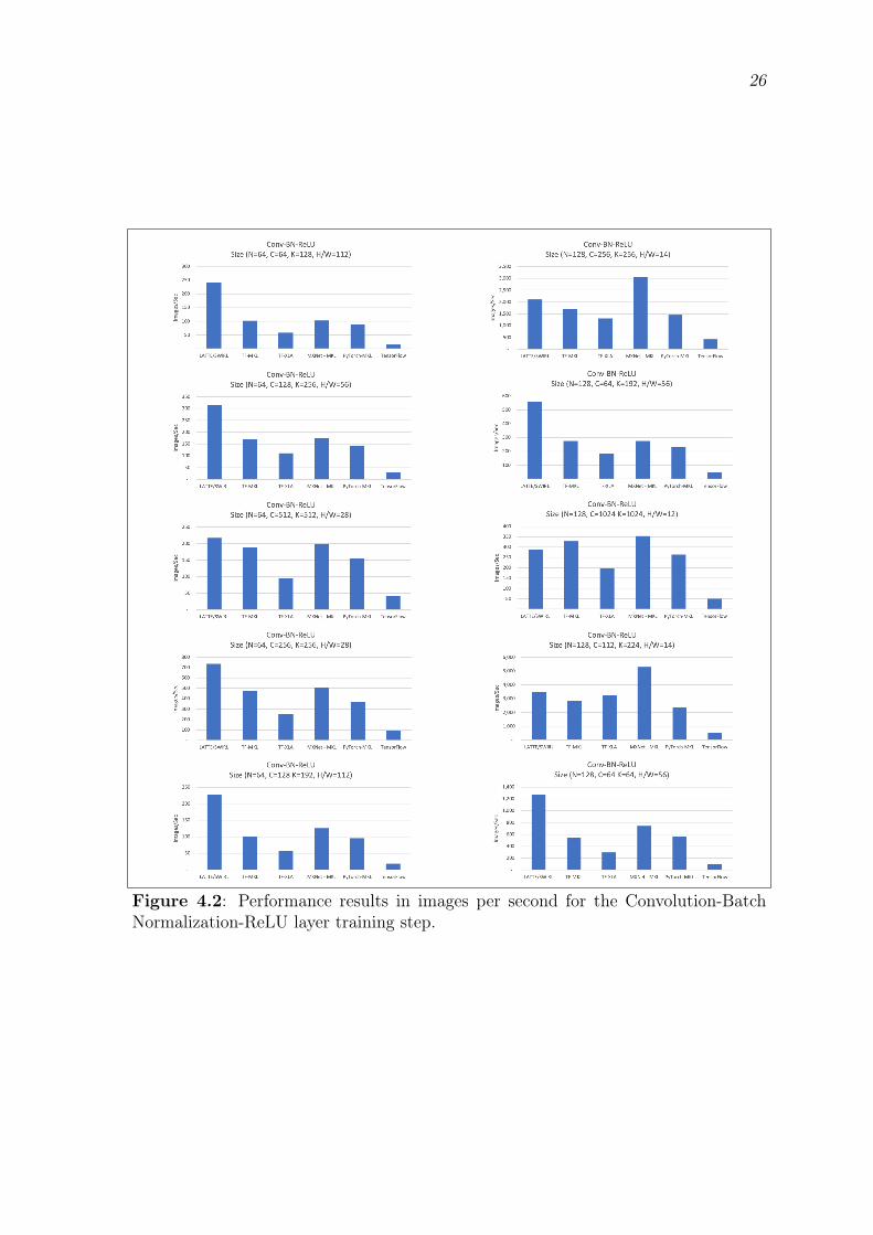
4.2 Performance results in images per second for the Convolution-BatchNormalization-ReLU layer training step. . . . . . . . . . . . . . . . . . . . . . . . . 26

4.3 Performance results in time (ms) for the Convolution-Batch Normalization-ReLU layer training step. Displays the time spent on each operator. . . 27

CHAPTER 1

INTRODUCTION

Deep Neural Networks (DNNs) are currently one of the fastest growing areas in com-

puter science, with wide-ranging applications from speech recognition to genomics.

DNNs are a class of models that use a system of interconnected neurons to estimate

or approximate functions. Typical DNNs, which consist of multiple stacked layers,

require billions of operations for training and inference. These networks are compute

intensive, and Graphics Processing Units (GPUs) have been the hardware of choice

for many neural networks. However, as the applicability of DNNs has increased,

the need for performance on different computing platforms has grown. Due to a

variety of factors, including cost and programming complexity, GPUs are not always

incorporated into many computing clusters. For example, many scientific applications

that employ neural networks are not run on HPC clusters that incorporate GPUs into

their architectures. Therefore, there is a demand for performance and portability of

DNNs across a variety of architectures and platforms.

Deep Neural Networks are composed of multiple layers, most often including fully-

connected, convolutional and activation layers. Many novel layers have been proposed

to increase performance and reduce training times. Batch Normalization (BN) is

one such layer that standardizes the inputs to other layers. This has the effect

of stabilizing the learning process and dramatically reducing the number of epochs

required to train deep networks. The use of BN layers in neural networks has quickly

become standard due to its effectiveness [2]. Convolutional and fully-connected

layers are typically some of the most computationally-intensive sections of the net-

works. Currently, BN is recognized as one of the most computationally intensive

non-convolution layers and is increasingly consuming a larger portion of the execution

2

time during training for many DNNs [3].

Because of their recent popularity, there are many frameworks that can train and run

DNNs. These high-level frameworks, such as TensorFlow [4], Torch [5], Theano [6],

Caffe [7], CNTK [8] and MXNet[9], use abstraction to represent neural networks and

employ one of three approaches: computation graph engines, layer-specific libraries,

and domain-specific languages. Most of these implementations use statically-tuned

libraries such as cuDNN for GPUs and Eigen or Intel MKL-DNN for CPUs to achieve

performance. cuDNN is a library of highly-tuned implementations for standard

routines used in deep neural networks, such as forward and backward convolution,

pooling, normalization, and activation layers [10]. Eigen is a high-level C++ library

of template headers for linear algebra, matrix and vector operations, geometrical

transformations, numerical solvers and related algorithms [11]. Intel MKL-DNN is

a performance-enhancing library for accelerating deep learning frameworks on Intel

architectures. MKL-DNN implements optimized operators that are common in DNN

models, including Convolution, Pooling, Batch Normalization, and Activation. [12].

Due to neural networks being very computationally expensive and involving latency-

critical tasks, generating efficient instructions for various platforms is challenging.

Preoptimized libraries provide various reliable and fast implementations for linear

algebra operations. However, these libraries lack optimization across operators, and

the execution of each operation varies dramatically for different data sizes, data lay-

outs, configurations for operators, memory hierarchies and specific hardware features.

When a new operator is developed for use in DNNs that does not fit into these

preoptimized library functions, the computation efficiency decreases dramatically [13].

Because of these challenges, compiler-based approaches have recently garnered more

interest for achieving performance in neural networks. Compiler-based approaches

can separate algorithms from schedules, which allows users to experiment with dif-

ferent options for parallelism and data locality on a wide range of platforms. This

approach was demonstrated by Halide. Halide is a domain-specific language for image

processing that decouples the algorithm definition from the execution strategy and

3

provides performance portability across different architectures [14].

LATTE is a domain-specific language for DNNs with a graph-like implementation

that uses a compiler-based approach for optimization. LATTE provides abstraction

to the user through the use of layers. The abstraction hides low-level details such as

parallelization, data layout optimizations and code generation from the user. This

allows the user to write neural network layers at a high level without architecture-

specific optimizations.

SWIRL is a domain-specific compiler for neural networks that can be used with

LATTE. SWIRL takes LATTE as input and produces optimized C++ code. Without

SWIRL, LATTE uses its own compiler that generates library calls. In contrast,

SWIRL uses high-level transformation recipes to generate efficient CPU code. These

transformation commands span both data and computation planes. For example,

the transformation commands can change the data layout for improved locality,

vectorization and parallelization. The layer transformation commands include clas-

sical compiler transformations such as tiling, unroll-and-jam and unroll. SWIRL has

demonstrated comparable performance with TensorFlow integrated with MKL-DNN

on both training and inference for a variety of neural networks, including AlexNet,

Overfeat and VGG [15]. Currently, LATTE does not have a Batch Normalization

operator. Extending LATTE to include this operator and SWIRL to generate opti-

mizations for this operator will broaden the efficacy and applicability of the LATTE

language and the SWIRL compiler for DNNs.

The key contributions of this thesis are:

• An extension of LATTE and SWIRL to include the BN operator and compiler

optimizations that can be applied to this operator.

• An application of scalar replacement for reduced memory access and loop in-

terchange and fusion for increased parallelism in the BN LATTE code imple-

mentation.

4

• A transformation recipe for SWIRL to create a SIMD vectorization and paral-

lelization strategy for optimizing BN in LATTE.

• A performance evaluation of the BN operator and of the combined Convolution-

BN-ReLU layer on the Intel SkyLake platform, comparing LATTE and SWIRL

to TensorFlow, PyTorch and MXNet all integrated with the MKL-DNN library,

TensowFlow XLA and native TensorFlow.

CHAPTER 2

BACKGROUND

This section provides a brief description of Batch Normalization and its benefits for

training DNNs. The compilation workflow of LATTE and SWIRL is described along

with details of how the Batch Normalization Layer is expressed in LATTE.

2.1 Batch NormalizationAdvances in deep learning research are largely driven by the introduction of novel

hidden layers and architectures. Batch Normalization is a technique introduced in [1]

that decreases the training time and increases the robustness of neural networks. Deep

neural networks are challenging to train, in part because the input from prior layers

can change after weight updates during each training pass. Because the inputs to each

layer are affected by the parameters of all preceding layers, this creates an amplifying

effect as the network depth increases. Internal covariate shift refers to the variability

in the distribution of network activations due to the change in network parameters

during training. This variance in the input distribution slows down the training by

requiring lower learning rates and careful parameter initialization. Because Batch

Normalization reduces the variance in the inputs and the activations in a network, it

can allow for higher learning rates during training. Traditionally, higher learning rates

are more likely to cause gradients to explode or vanish, which leads to the network

getting stuck in local minima during training. Because Batch Normalization reduces

the variability in inputs, it prevents small changes to the parameters from amplifying

into larger and suboptimal changes in activations for gradients. This reduces the time

for convergence.

Covariate shift also makes training difficult with saturating activation functions, such

as sigmoid and tanh. Because of the higher variance in inputs, it is more likely that

6

the input will move into the saturated regime of the nonlinear activation function and

slow down convergence. Batch Normalization decreases the variability of the inputs

to the nonlinear activation functions, making them more stable and less likely to

become saturated, which accelerates the training of the network. The BN transform

has been shown to decrease training time and to match performance on many popular

DNN models [16]. Because of its proven benefits in training DNNs, its use has become

rather ubiquitous in many neural networks today.

While its ability to accelerate the training process in DNNs is not necessarily disputed,

the reason for Batch Normalization’s effectiveness has been challenged in recent

literature. For instance, the link between the performance gain of BN and the

reduction of internal covariate shift has been questioned. In [17], the benefits of

BN are demonstrated to be a result of smoothing the objective function. This

smoothing creates more predictive gradients and allows for lower learning rates and

faster convergence. In [18], the authors argue that the success of Batch Normalization

is due to optimizing the length and direction of the parameters separately, which

creates a more favorable loss landscape for gradient-based methods.

2.1.1 Batch Normalization Transform

Batch Normalization is achieved through a normalization step that fixes the means

and variances of each layer’s inputs. Each dimension of the input data is normalized

to a mean of zero and a standard deviation of one. The BN transform is performed

on mini-batches since these are used during stochastic gradient training. Therefore,

the mean and variation of each input dimension are calculated over a mini batch

B. Normalizing each input of a layer may change what the layer can represent. To

address this, the BN transform includes a pair of parameters, � and �, which scale

and shift the normalized values. These parameters are learned during training. The

full Batch Normalization transform algorithm is shown in Figure 2.1.

Equation 1 calculates the mean of a mini-batch B with m inputs. Equation 2

7

Input: Values of x over a mini-batch: B = {x1...xm};Parameters to be learned: �, �

Output: {yi = BN�,�(xi)}

µB 1

m

mX

i=1

xi // mini-batch mean (1)

�2B

1

m

mX

i=1

(xi � µB)2 // mini-batch variance (2)

bxi xi � µBp�2B + ✏

// normalize (3)

yi � bxi + � ⌘ BN�,�(xi) // scale and shift (4)

Figure 2.1: Algorithm for Batch Normalization Transform. Taken from [1]

calculates the variance by subtracting the mean, µB, from each input value and

squaring this difference. The variance is also calculated over the mini-batch B.

Equation 3 normalizes the inputs to be centered at 0 with a standard deviation

of 1. Epsilon is a constant and is added for numerical stability. Equation 4 scales the

normalized inputs by � and shifts them by �.

The BN transform can be added to a network to manipulate any activation. Batch

Normalization may be used on the inputs to the layer before or after the activation

function in the previous layer. It may be more appropriate after the activation

function for S-shaped functions like the hyperbolic tangent and logistic function.

For activation functions that can result in non-Gaussian distributions, such as the

rectified linear activation function (ReLU), the BN transform is often applied before

the activation function [1].

2.1.2 Back Propagation

If the BN transform is computed outside the gradient step, the model parameters

can blow up and hinder training. Therefore, an important piece of the Batch Nor-

malization technique is allowing the gradient of the loss with respect to the model

parameters to account for the normalization. The BN transform is differentiable, and

8

the gradient of the loss with respect to the different parameters can be computed

directly with the chain rule.

�`

� bxi=

�`

�yi· � (1)

�`

��2B=

mX

i=1

�`

� bxi· (xi � µB) ·

�12(�2

B + ✏)�3/2 (2)

�`

�µB=

✓ mX

i=1

�`

� bxi· �1p

�2B + ✏

◆+

�`

��2B·Pm

i=1�2(xi � µB)

m(3)

�`

�xi=

�`

� bxi· 1p

�2B + ✏

+�`

��2B· 2(xi � µB)

m+

�`

�µB· 1

m(4)

�`

��=

mX

i=1

�`

�yi· bxi (5)

�`

��=

mX

i=1

�`

�yi(6)

Figure 2.2: Backpropagation for the Batch Normalization Transform

The equations shown in Figure 2.2 represent the backward pass of a Batch Nor-

malization training step. The gradient with respect to the normalized inputs, �`� bxi

,

is computed in Equation 1. The gradients for � and � ( �`�� ,

�`�� ) are calculated in

Equations 5 and 6 respectively.

2.2 LATTE and SWIRLLATTE is a domain-specific language for DNNs that provides abstraction for the

user to create a neural network, and SWIRL uses high-level transformation recipes to

generate efficient CPU code. The transformation recipe abstraction allows an expert

programmer to explicitly enumerate the transformations that can be applied to each

individual layer within LATTE. The main SWIRL transformations used for the BN

operator include tiling, loop unrolling, vectorization and parallelization. Tiling can

improve cache locality. Unrolling certain loop iterations by a factor reduces branch

penalties and improves register reuse. Vectorization creates intrinsics to be used on

SIMD architectures, and parallelization uses OpenMP to parallelize one or more loops

9

for increased performance. These optimizations can be tailored for performance on a

variety of CPU backends [15].

A DNN is created in LATTE by stacking layers on top of each other, starting with

an input layer, adding various hidden layers and ending with a fully-connected layer

that applies an activation function. These layers are represented as ensembles of

neurons that are connected using mapping functions [19]. LATTE uses an implicit

data-flow graph model of the DNN. The nodes represent computations in layers, and

the edges are data dependencies between layer inputs and outputs. This data-flow

graph is represented by a dictionary of mapping functions, which connects the inputs

and outputs of layers. This allows LATTE to store complex graphs without incurring

extra memory costs. For training and inference, SWIRL generates kernels for com-

putations as a set of nested for-loops for each forward, backward and weight update

pass of each layer.

Figure 2.3 shows a Python code sequence for expressing Batch Normalization in

LATTE. The BatchNormLayer function takes three arguments: the network object

(net), the input ensemble (input_ensemble) and epsilon. The neurons are created

in Line 8 and added to the BN ensemble in Line 10. A mapping function is defined

on Lines 13-14 which connects the input_ensemble to the bn_ensemble.

Once the user has defined a neural network in LATTE, the description is then lowered

to a standard Python AST. Next, the SWIRL compiler uses transformation recipes

on the Python AST. Lastly, the transformed Python AST is translated to C++ code

using the ctree package, which is then lowered to optimized x86 machine code using

the Intel C++ Compiler. High-quality vector code is also generated via intrinsics

rather than relying on compiler directives. See Figure 2.4 for a visual representation

of this workflow.

10

1 def BatchNormLayer(net, input_ensemble, epsilon=0.001):2 input_channels, input_height, input_width = input_ensemble.shape3 shape = (input_channels, input_height, input_width)4 neurons = np.empty(shape, dtype=’object’)5 batch_num = net.batch_size67 #Create an ensemble and initialize it8 neurons[:,:,:] = BNNeuron(input_ensemble, batch_num, epsilon)9 bn_ensemble = BNEnsemble(neurons)

10 net.add_ensemble(bn_ensemble)1112 #Mapping function for add_connections13 def mapping(c,x,y):14 return (range(c), range(x), range(y))15 net.add_connections(input_ensemble, bn_ensemble, mapping)

Figure 2.3: Python Code for Batch Normalization Layer in LATTE

Figure 2.4: LATTE/SWIRL Workflow

CHAPTER 3

METHODS

The pseudo code for the Batch Normalization transform, backpropagation and pa-

rameter updates is described and shown in Figures 3.1-3.3. These loops can be

optimized in a number of ways. Some general optimization techniques, such as scalar

replacement combined with loop interchange and loop fusion, were performed on the

code directly within LATTE. SWIRL transformation recipes were used for the rest

of the optimizations. These are discussed in more detail in this section.

3.1 Batch Normalization in Pseudo CodeThe Batch Normalization transform, represented by the equations in Figure 2.1,

is expressed by the loop nests in Figure 3.1. Since the transform is applied to

mini-batches, the batch dimension N is used. The mean and variance are calculated

per feature map or channel dimension C, as shown in Lines 6 and 16 of Figure 3.1.

The heights and widths of the inputs are H and W respectively. The normalized

inputs are referenced as x_hat on Line 26 and are scaled by gamma and shifted by

beta on Line 27. The inputs and outputs are x and y respectively.

Figure 3.2 displays the loop nests that express the backpropagation step of Batch

Normalization. Because the transform is computed in mini-batches, the gradient is

calculated in mini-batches as well. The mini-batch size is N . The gradient flowing

from the prior layer (ry) is grad, andrx is grad_x. The gradients for the mini-batch

mean and variance (rµB,r�2B) are dmu and dvar respectively. The other variables are

for ease in computing the gradients. After a series of steps, the gradient with respect

to the normalized inputs (referenced as grad_x) is calculated on Line 30 of Figure 3.2.

Figure 3.3 shows the loops nests for the parameter updates of gamma and beta. Sim-

12

1 //Calculate the mean per channel dimension2 for (n=0; n < N; n++) { // mini-batch size3 for(c=0; c < C; c++) { //channel dimension4 for(h=0; h < H; h++) { //height5 for(w=0; w < W; w++) { //width6 mean[c] += x[n,c,h,w]7 } } } }8 for(c=0; c < C; c++) {9 mean[c] = mean[c] / (N * H * W) }

1011 //Calculate the variance per channel dimension12 for (n=0; n < N; n++) {13 for(c=0; c < C; c++) {14 for(h=0; h < H; h++) {15 for(w=0; w < W; w++) {16 var[c] += (x[n,c,h,w]-mean[c])*(x[n,c,h,w]-mean[c])17 } } } }18 for(c=0; c < C; c++) {19 var[c] = var[c] / (N * H * W) }2021 //Apply batch normalization transform22 for (n=0; n < N; n++) {23 for(c=0; c < C; c++) {24 for(h=0; h < H; h++) {25 for(w=0; w < W; w++) {26 x_hat[n,c,h,w] = (x[n,c,h,w] - mean[c]) / sqrt(var[c] +

,! epsilon)27 y[n,c,h,w] = gamma[c] * x_hat[n,c,h,w] + beta[c]28 } } } }

Figure 3.1: Batch Normalization Forward Pass

13

1 //Calculate the gradient with respect to the variance on dimension C2 for (n=0; n < N; n++){3 for(c=0; c < C; c++) {4 for(h=0; h < H; h++) {5 for(w=0; w < W; w++) {6 divar[c] += grad[n,c,h,w] * gamma[c] * (x[n,c,h,w] -

,! mean[c])7 } } } }8 for(c=0; c < C; c++) {9 dsqrtvar[c] = -1.0 / (var[c] + epsilon) * divar[c]

10 dvar[c] = 0.5 / sqrt(var[c] + epsilon) * dsqrtvar[c]11 }1213 //Calculate the gradient with respect to the mean on dimension C14 for (n=0; n < N; n++) {15 for(c=0; c < C; c++) {16 for(h=0; h < H; h++) {17 for(w=0; w < W; w++) {18 dxmu1 = grad[n,c,h,w] * gamma[c] / sqrt(var[c] +

,! epsilon)19 dxmu2 = 2.0 * (x[n,c,h,w]- mean[c]) / (N * H * W) *

,! dvar[c]20 dx1[n,c,h,w] = dxmu1 + dxmu221 dmu[c] -= dx1[n,c,h,w]22 } } } }2324 //Calculate the gradient with respect to the inputs25 for (n=0; n < N; n++) {26 for(c=0; c < C; c++) {27 for(h=0; h < H; h++) {28 for(w=0; w < W; w++) {29 dx2[n,c,h,w] = dmu[c] / (N * H * W)30 grad_x[n,c,h,w] = dx1[n,c,h,w] + dx2[n,c,h,w]31 } } } }

Figure 3.2: Batch Normalization Back Propagation

14

ilar to the mean and variance, gamma and beta are calculated per channel dimension

C. Line 6 computes the gradient for gamma, grad_gamma, and Line 7 shows the

gradient calculation for beta, grad_beta.

1 //Calculate the gradient with respect to the beta and gamma parameters2 for (n=0; n < N; n++) {3 for(c=0; c < C; c++) {4 for(h=0; h < H; h++) {5 for(w=0; w < W; w++) {6 grad_gamma[c] += grad[n,c,h,w] * x_hat[n,c,h,w]7 grad_beta[c] += grad[n,c,h,w]8 } } } }

Figure 3.3: Batch Normalization Parameter Update

3.2 Scalar ReplacementThe goal of scalar replacement is to identify repeated accesses made to the same

memory address, either within an iteration or across iterations, and to remove the

redundant accesses by keeping the data in registers. Compilers are effective in allo-

cating scalar variables to registers but often fail to do so with array references. Data

dependences provide opportunities for reuse of array variables in registers through

scalar replacement [13, Chapter 8].

All of the loop nests shown in Figures 3.1-3.3 exhibit data dependences that can be

exploited through scalar replacement. For example, in Figure 3.1 the array reference

on Line 6 for mean has both an output and a true dependence carried by all but the

C loop. Line 16 has similar dependences for the array reference to var and also an

input dependence for the array reference to mean carried by all of the loops except

C. In the last loop nest structure, there are input dependences for mean and var on

line 26 and gamma and beta on line 27 carried by all of the loops except C. Lastly,

there is a loop-independent true dependence for x_hat on line 27.

15

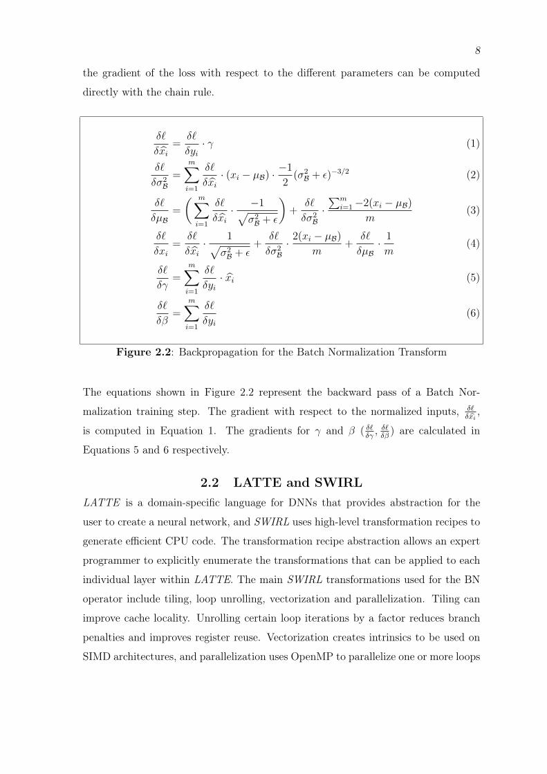
Figure 3.4 reflects the changes made for scalar replacement in the Batch Normal-

ization forward pass. To fully exploit the benefits of the scalar replacement, loop

interchange of the C and N loops is performed. Because the C loop does not carry

any dependences, moving the N loop inside of the C loop allows for more reuse of the

values by keeping them in registers during the iterations of the N , H and W loops.

Since the C loop is now the outermost loop and does not carry any dependences, all

of the C loops can be fused. This fusion can increase the level of parallelism and data

locality that can be exploited in the compiler transformations applied to this code

by SWIRL. It also decreases the loop control overhead. Lastly, a final optimization

technique is used for the expensive square root and division operations shown on

Line 26 of Figure 3.1. This operation is an input dependence carried in the C loop,

which means that this time-consuming calculation needs only to be performed once

per C loop iteration rather than for each iteration of every loop. A multiplication

operator replaces the more expensive division operator. On Line 21 of Figure 3.4

these calculations are stored in a register and reused on Line 26.

The backward pass exhibits even more opportunities for register reuse. The array

reference on Line 6 of Figure 3.2 for divar has both an output and a true dependence

carried by all but the C loop. Input dependences for the array references to gamma

and mean on Line 6 are carried by all but the C loop as well. Line 8 displays a

loop-independent true dependence on the reference to dsqrtvar and Lines 8-9 have

an input dependence on var. In the third loop nest, input dependences are carried

by all but the C loop for gamma, var, mean and dvar. On Line 21, dmu exhibits the

same dependences as divar does above on Line 6. The last loop nest carries an input

dependence on dmu on Line 29.

Scalar replacements are performed for each of the dependences listed above. As was

done in the forward pass, the C and N loops are interchanged and all the C loops are

fused. Expensive operations that are input dependences are replaced with scalars in

lines 12-14 and 29 of Figure 3.5, which shows the optimized loops nests.

16

1 for(c=0; c < C; c++) {2 mean_temp = 0.03 var_temp = 0.04 gamma_temp = gamma[c]5 beta_temp = beta[c]6 for (n=0; n < N; n++) {7 for(h=0; h < H; h++) {8 for(w=0; w < W; w++) {9 mean_temp += x[n,c,h,w]

10 } } }11 mean_temp = mean_temp / (N * C * W)12 mean[c] = mean_temp1314 for (n=0; n < N; n++) {15 for(h=0; h < H; h++) {16 for(w=0; w < W; w++) {17 var_temp += x[n,c,h,w] - mean_temp18 } } }19 var_temp = var_temp / (N * C * W)20 var[c] = var_temp21 divisor = 1 / sqrt(var_temp + epsilon)2223 for (n=0; n < N; n++) {24 for(h=0; h < H; h++) {25 for(w=0; w < W; w++) {26 x_hat_temp = (x[n,c,h,w] - mean_temp) * divisor27 y[n,c,h,w] = gamma_temp * x_hat_temp + beta_temp28 x_hat[n,c,h,w] = x_hat_temp29 } } } }

Figure 3.4: Batch Normalization Forward Pass with Scalar Replacement Optimiza-tions

The parameter update loop nest shown in Figure 3.3 is optimized in a similar manner

in Figure 3.6. Lines 6 and 7 have output and true and dependences carried by all

but the C loop nests for grad_gamma and grad_beta respectively. Additionally, Lines

6 and 7 show loop-independent input dependences for grad. These array references

are replaced with scalar variables, and the C and N loops are interchanged. All of

the transformations described in Figures 3.4 to 3.6 were expressed within the LATTE

language. The rest of the optimizations were performed using the SWIRL compiler.

17

1 for(c=0; c < C; c++) {2 divar = 0.03 gamma_temp = gamma[c]4 mean_temp = mean[c]5 var_temp = var[c]6 //Calculate the gradient with respect to the variance on dimension

,! C7 for (n=0; n < N; n++){8 for(h=0; h < H; h++) {9 for(w=0; w < W; w++) {

10 divar += grad[n,c,h,w] * gamma_temp * (inputs[n,c,h,w],! - mean_temp)

11 } } }12 inver = 1.0 / sqrt(var_temp + epsilon)13 dvar_temp = -0.5 * inver / (var_temp + epsilon) * divar14 inver_dvar = 1.0 / (N * H * W) * dvar_temp1516 //Calculate the gradient with respect to the mean on dimension C17 for (n=0; n < N; n++) {18 for(h=0; h < H; h++) {19 for(w=0; w < W; w++) {20 dxmu1 = grad[n,c,h,w] * gamma_temp21 * inver22 dxmu2 = 2.0 * (inputs[n,c,h,w]- mean_temp) * inver_dvar23 dx1_temp = dxmu1 + dxmu224 dx1[n,c,h,w] = dx1_temp25 dmu += - dx1_temp26 } } }2728 //Calculate the gradient with respect to the inputs29 inver_dmu = 1 / (N * C * W) * dmu30 for (n=0; n < N; n++) {31 for(h=0; h < H; h++) {32 for(w=0; w < W; w++) {33 dx2[n,c,h,w] = dmu / N34 grad_x[n,c,h,w] = dx1[n,c,h,w] + inver_dmu35 } } } }

Figure 3.5: Batch Normalization Back Propagation with Scalar Replacement Opti-mizations

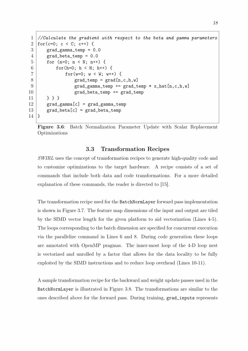
18

1 //Calculate the gradient with respect to the beta and gamma parameters2 for(c=0; c < C; c++) {3 grad_gamma_temp = 0.04 grad_beta_temp = 0.05 for (n=0; n < N; n++) {6 for(h=0; h < H; h++) {7 for(w=0; w < W; w++) {8 grad_temp = grad[n,c,h,w]9 grad_gamma_temp += grad_temp * x_hat[n,c,h,w]

10 grad_beta_temp += grad_temp11 } } }12 grad_gamma[c] = grad_gamma_temp13 grad_beta[c] = grad_beta_temp14 }

Figure 3.6: Batch Normalization Parameter Update with Scalar ReplacementOptimizations

3.3 Transformation RecipesSWIRL uses the concept of transformation recipes to generate high-quality code and

to customize optimizations to the target hardware. A recipe consists of a set of

commands that include both data and code transformations. For a more detailed

explanation of these commands, the reader is directed to [15].

The transformation recipe used for the BatchNormLayer forward pass implementation

is shown in Figure 3.7. The feature map dimensions of the input and output are tiled

by the SIMD vector length for the given platform to aid vectorization (Lines 4-5).

The loops corresponding to the batch dimension are specified for concurrent execution

via the parallelize command in Lines 6 and 8. During code generation these loops

are annotated with OpenMP pragmas. The inner-most loop of the 4-D loop nest

is vectorized and unrolled by a factor that allows for the data locality to be fully

exploited by the SIMD instructions and to reduce loop overhead (Lines 10-11).

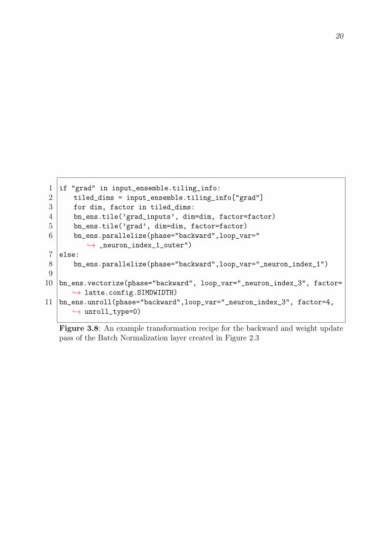
A sample transformation recipe for the backward and weight update passes used in the

BatchNormLayer is illustrated in Figure 3.8. The transformations are similar to the

ones described above for the forward pass. During training, grad_inputs represents

19

1 if "value" in input_ensemble.tiling_info:2 tiled_dims = input_ensemble.tiling_info["value"]3 for dim, factor in tiled_dims:4 bn_ens.tile(’inputs’, dim=dim, factor=factor)5 bn_ens.tile(’value’, dim=dim, factor=factor)6 bn_ens.parallelize(phase="forward",loop_var="

,! _neuron_index_1_outer")7 else:8 bn_ens.parallelize(phase="forward",loop_var="_neuron_index_1")9

10 bn_ens.vectorize(phase="forward", loop_var="_neuron_index_3", factor=,! latte.config.SIMDWIDTH)

11 bn_ens.unroll(phase="forward",loop_var="_neuron_index_3", factor=4,,! unroll_type=0)

Figure 3.7: An example transformation recipe for the forward pass of the BatchNormalization layer created in Figure 2.3.

the input gradients and grad represents the output gradients of the current ensemble

layer. The feature map dimensions of the grad_input and grad are tiled by the

SIMD vector length for the given platform to aid vectorization (Lines 4-5). The loops

corresponding to the batch dimension are specified for parallelization for both the

backward and weight update loops via the parallelize command in Lines 6 and 8.

The inner-most loop is vectorized and unrolled as shown in Lines 10-11.

Applying the transformation recipes in Figures 3.7 and 3.8 to the Batch Normalization

layer in LATTE generates optimized code for the Intel SkyLake platform. The final

C++ code generated by the SWIRL compiler for the forward pass is shown in Figure

3.9.

20

1 if "grad" in input_ensemble.tiling_info:2 tiled_dims = input_ensemble.tiling_info["grad"]3 for dim, factor in tiled_dims:4 bn_ens.tile(’grad_inputs’, dim=dim, factor=factor)5 bn_ens.tile(’grad’, dim=dim, factor=factor)6 bn_ens.parallelize(phase="backward",loop_var="

,! _neuron_index_1_outer")7 else:8 bn_ens.parallelize(phase="backward",loop_var="_neuron_index_1")9

10 bn_ens.vectorize(phase="backward", loop_var="_neuron_index_3", factor=,! latte.config.SIMDWIDTH)

11 bn_ens.unroll(phase="backward",loop_var="_neuron_index_3", factor=4,,! unroll_type=0)

Figure 3.8: An example transformation recipe for the backward and weight updatepass of the Batch Normalization layer created in Figure 2.3

21

1 #pragma omp parallel for2 for (int _neuron_index_1 = 0; _neuron_index_1 < 2; _neuron_index_1 += 1) {3 __m512 mean_temp_0 = _mm512_set1_ps(0.0);4 __m512 mean_temp_1 = _mm512_set1_ps(0.0);5 __m512 mean_temp_2 = _mm512_set1_ps(0.0);6 __m512 mean_temp_3 = _mm512_set1_ps(0.0);7 double mean_t1 = 0.0;8 for (int _neuron_index_0 = 0; _neuron_index_0 < 2; _neuron_index_0 += 1) {9 for (int _neuron_index_2 = 0; _neuron_index_2 < 64; _neuron_index_2 += 1) {

10 for (int _neuron_index_3 = 0; _neuron_index_3 < 64; _neuron_index_3 += 64) {11 mean_temp_0 = _mm512_add_ps(mean_temp_0, _mm512_load_ps(& inputs[_neuron_index_0][

,! _neuron_index_1][_neuron_index_2][(_neuron_index_3 + 0)]));12 mean_temp_1 = _mm512_add_ps(mean_temp_1, _mm512_load_ps(& inputs[_neuron_index_0][

,! _neuron_index_1][_neuron_index_2][(_neuron_index_3 + 16)]));13 mean_temp_2 = _mm512_add_ps(mean_temp_2, _mm512_load_ps(& inputs[_neuron_index_0][

,! _neuron_index_1][_neuron_index_2][(_neuron_index_3 + 32)]));14 mean_temp_3 = _mm512_add_ps(mean_temp_3, _mm512_load_ps(& ensemb le2inputs[_neuron_index_0][

,! _neuron_index_1][_neuron_index_2][(_neuron_index_3 + 48)] ));15 } } }16 mean_t1 += _mm512_reduce_add_ps(_mm512_div_ps(mean_temp_0, _mm512_set1_ps(8192)));17 mean_t1 += _mm512_reduce_add_ps(_mm512_div_ps(mean_temp_1, _mm512_set1_ps(8192)));18 mean_t1 += _mm512_reduce_add_ps(_mm512_div_ps(mean_temp_2, _mm512_set1_ps(8192)));19 mean_t1 += _mm512_reduce_add_ps(_mm512_div_ps(mean_temp_3, _mm512_set1_ps(8192)));20 mean[_neuron_index_1] = mean_t1;21 __m512 mean_t2 = _mm512_set1_ps(mean[_neuron_index_1]);22 __m512 var_temp_0 = _mm512_set1_ps(0.0);23 __m512 var_temp_1 = _mm512_set1_ps(0.0);24 __m512 var_temp_2 = _mm512_set1_ps(0.0);25 __m512 var_temp_3 = _mm512_set1_ps(0.0);26 double var_t = 0.0;27 for (int _neuron_index_0 = 0; _neuron_index_0 < 2; _neuron_index_0 += 1) {28 for (int _neuron_index_2 = 0; _neuron_index_2 < 64; _neuron_index_2 += 1) {29 for (int _neuron_index_3 = 0; _neuron_index_3 < 64; _neuron_index_3 += 64) {30 __m512 diff_0 = _mm512_sub_ps(_mm512_load_ps(& inputs[_neuron_index_0][_neuron_index_1][

,! _neuron_index_2][(_neuron_index_3 + 0)]), mean_t2);31 __m512 diff_1 = _mm512_sub_ps(_mm512_load_ps(& 2inputs[_neuron_index_0][_neuron_index_1][

,! _neuron_index_2][(_neuron_index_3 + 16)]), mean_t2);32 __m512 diff_2 = _mm512_sub_ps(_mm512_load_ps(& 2inputs[_neuron_index_0][_neuron_index_1][

,! _neuron_index_2][(_neuron_index_3 + 32)]), mean_t2);33 __m512 diff_3 = _mm512_sub_ps(_mm512_load_ps(& inputs[_neuron_index_0][_neuron_index_1][

,! _neuron_index_2][(_neuron_index_3 + 48)]), mean_t2);34 var_temp_0 = _mm512_fmadd_ps(diff_0, diff_0, var_temp_0);35 var_temp_1 = _mm512_fmadd_ps(diff_1, diff_1, var_temp_1);36 var_temp_2 = _mm512_fmadd_ps(diff_2, diff_2, var_temp_2);37 var_temp_3 = _mm512_fmadd_ps(diff_3, diff_3, var_temp_3);38 } } }3940 var_t += _mm512_reduce_add_ps(_mm512_div_ps(var_temp_0, _mm512_set1_ps(8192)));41 var_t += _mm512_reduce_add_ps(_mm512_div_ps(var_temp_1, _mm512_set1_ps(8192)));42 var_t += _mm512_reduce_add_ps(_mm512_div_ps(var_temp_2, _mm512_set1_ps(8192)));43 var_t += _mm512_reduce_add_ps(_mm512_div_ps(var_temp_3, _mm512_set1_ps(8192)));44 var[_neuron_index_1] = var_t;45 __m512 gamma_temp = _mm512_set1_ps(gamma[_neuron_index_1]);46 __m512 beta_temp = _mm512_set1_ps(beta[_neuron_index_1]);47 __m512 divisor = _mm512_set1_ps(1.0 / sqrt(var_t + 0.001));48 for (int _neuron_index_0 = 0; _neuron_index_0 < 2; _neuron_index_0 += 1) {49 for (int _neuron_index_2 = 0; _neuron_index_2 < 64; _neuron_index_2 += 1) {50 for (int _neuron_index_3 = 0; _neuron_index_3 < 64; _neuron_index_3 += 64) {51 __m512 x_hat_0 = _mm512_mul_ps(_mm512_sub_ps(_mm512_load_ps(& inputs[_neuron_index_0][

,! _neuron_index_1][_neuron_index_2][(_neuron_index_3 + 0)]), mean_t2), divisor);52 __m512 x_hat_1 = _mm512_mul_ps(_mm512_sub_ps(_mm512_load_ps(& inputs[_neuron_index_0][



,! _neuron_index_1][_neuron_index_2][(_neuron_index_3 + 48)]), mean_t2), divisor);55 _mm512_store_ps(& x_hat[_neuron_index_0][_neuron_index_1][_neuron_index_2][(_neuron_index_3 + 0)],

,! x_hat_0);56 _mm512_store_ps(& x_hat[_neuron_index_0][_neuron_index_1][_neuron_index_2][(_neuron_index_3 + 16)],



,! x_hat_3);59 _mm512_store_ps(& value[_neuron_index_0][_neuron_index_1][_neuron_index_2][(_neuron_index_3 + 0)],

,! _mm512_fmadd_ps(gamma_temp, x_hat_0, beta_temp));60 _mm512_store_ps(& value[_neuron_index_0][_neuron_index_1][_neuron_index_2][(_neuron_index_3 + 16)],



,! _mm512_fmadd_ps(gamma_temp, x_hat_3, beta_temp));63 } } } };

Figure 3.9: Generated C++ code from the SWIRL transformation recipe shown inFigure 3.7

CHAPTER 4

RESULTS

The performance results of using LATTE and SWIRL for the Batch Normalization

layer compared to other state-of-the-art frameworks is described in this section. The

results were generated on an Intel Skylake platform with AVX-512 support. The

frameworks used for comparison include TensorFlow release version 1.11.0, Ten-

sorFlow release version 2.0.0 configured with Intel Math Kernel Library (MKL),

TensorFlow relsease version 2.0.0 using XLA, MXNet version 1.5.1 with MKL, and

Pytorch version 1.4.0+cpu with MKL.

4.1 Hardware Platform and EnvironmentThe hardware platform used is a high performance server class dual socket Intel Xeon

Gold 6130 SkyLake processor with 2 ⇥ 32 2.1 Ghz (max 3.7 Ghz) turbo-enabled cores.

This is an AVX-512 platform with 512-bit vector support. The processor has 98 GB

of DDR4-2666 memory, with 32KB of L1 cache, 1MB of L2 cache and 22MB of L3

Cache. The code is generated via the Intel C++ Compiler (ICC) v18.0.1.163 with

"-O3 -qopenmp -xCORE-AVX512" flags and NUM_OMP_THREADS=32.

4.2 Performance Comparison of Batch NormalizationThe performance of the LATTE/SWIRL implementation of the BN operator used

for training is compared with the five frameworks described above: TensorFlow,

TensorFlow with MKL-DNN, TensorFlow using XLA, MXNet with MKL-DNN, and

PyTorch with MKL-DNN. The training step involves a forward, backward and weight

update pass. The testing is carried out on ten different input sizes. The dimensions

of these input layers are representative of the sizes found in GoogleNet[20], VGGNet

[21] and ResNet[22] architectures. The results are displayed in Figure 4.1, comparing

23

the number of images per second each implementation can process with a batch size

of 64 and the image size listed as C, H/W where C represents the number of channels

and H/W represent the height and width dimensions respectively. LATTE/SWIRL

outperforms all of the other frameworks. On average, LATTE/SWIRL has 2x greater

throughput than MXNet with MKL-DNN, 4x more throughput than PyTorch with

MKL-DNN, 5x greater throughput than TensorFlow using XLA, 6x more throughput

than TensorFlow with MKL-DNN and 100x greater throughput than TensowFlow.

Figure 4.1: Performance results and breakdown for the Batch Normalization trainingstep. Demonstrates the effects of different optimizations towards overall performancefor the LATTE/SWIRL implementation.

24

The code optimizations shown in Figures 3.4-3.5 and the transformation recipes

shown in Figures 3.6-3.7 incorporate several compiler optimizations, including scalar

replacement, loop unrolling, SIMD vectorization and parallelization. The individual

effects of each optimization on the LATTE/SWIRL implementation are included in

the performance results of the Batch Normalization operator in Figure 4.1. The

breakdown is shown only for LATTE/SWIRL results, with the blue area representing

the baseline performance, the orange area displaying the performance with scalar

replacement included, the grey area showing the performance with the loop un-

rolling and SIMD vectorization in addition to scalar replacement, and the gold area

exhibiting the performance with all of the optimizations, including parallelization.

Scalar replacement achieves an increase between 4% to 18% , with an average of

15%. The loop unrolling and SIMD vectorization boost performance between 2%

and 11%, with an average of 9% and parallelization provides the greatest benefit by

improving performance from 69% to 93%, with an average increase of 77%. The

baseline performance of LATTE/SWIRL is roughly 2x better than the TensorFlow

implementation without MKL-DNN.

4.3 Performance Comparison for Conv-BN-ReLU LayerA comparison is presented for a training layer composed of Convolution, Batch

Normalization and ReLU activation operators. This layer configuration is commonly

found in many deep learning architectures and is suggested in [1]. The layer di-

mensions are representative of layers found in the GoogleNet[20], VGGNet [21] and

ResNet[22] architectures. The results can be seen in Figures 4.2 and 4.3. Figure 4.2

shows the images per second that each implementation can process with batch sizes

of either 64 or 128 with varying image sizes. C represents the number of in-channels

for the convolution layer, K represents the out-channels for the Convolution operator

and hence the number of channels for the BN and ReLU operators, and H/W are

the height and width respectively of the image for all of the operators. Figure 4.3

displays a time comparison for computing the Conv-BN-ReLU layer. This comparison

is presented so a breakout of the performance of each operator can be observed. Note

that the results from the native TensorFlow implementation are not included so the

25

graph would not be distorted, and the information from the other frameworks could

be seen more easily.

LATTE/SWIRL outperforms the other implementations on most of the tests. For

those dimensions where H/W is small (<=14), the Convolution operator in LAT-

TE/SWIRL is not as efficient as the Convolution operator in TensorFlow with MKL

and MXNet with MKL. The largest performance gains by LATTE/SWIRL are ob-

served for the test dimensions where H/W is large (i.e. 112). This demonstrates

that the loop unrolling and SIMD vectorization in LATTE/SWIRL on the inner

dimensions can be more fully exploited when the inner dimensions are large. For all

of the test sizes, LATTE/SWIRL was more efficient than the other frameworks for

the BN and ReLU activation operators.

26

Figure 4.2: Performance results in images per second for the Convolution-BatchNormalization-ReLU layer training step.

27

Figure 4.3: Performance results in time (ms) for the Convolution-BatchNormalization-ReLU layer training step. Displays the time spent on each operator.

CHAPTER 5

RELATED WORK

Compiler-based approaches are gaining more interest in the quest for performance

and portability of DNNs, which means that more compiler-based frameworks are

being introduced. TensorFlow’s XLA [23] compiles neural networks for CPUs, GPUs

and accelerators. It lowers nodes into primitive linear algebra operations and then

calls a backend-specific library for different architectures (such as Eigen for CPUs,

or cuDNN for GPUs) to perform the bulk of the computation. It aims to provide

backend flexibility for TensorFlow.

TVM [24] is a compiler that exposes graph-level and operator-level optimizations. It

lowers the traditional neural network dataflow graph into a two-phase internal repre-

sentation (IR). The high-level IR is optimized independent of the target architecture.

Then it lowers nodes into a low-level Halide-based internal representation wherein

loop-based optimizations can be performed. Halide is used to generate LLVM or

CUDA/Metal/OpenCL source code. TVM relies on an inventory of optimization

recipes. When an input layer’s parameters match one of those in the inventory,

the optimizations are invoked. Currently, TVM does not have support for training

operations, only inference.

Glow [25] is a machine learning compiler for heterogeneous hardware. Similar to

TVM, it uses a two-phase IR. The high-level internal representation allows the op-

timizer to perform domain-specific optimizations. The lower-level IR permits the

compiler to perform memory-related optimizations. Glow then calls optimized linear

algebra libraries in the lower-level IR. It is similar to TVM in that uses a compu-

tational graph engine for the high-level representation, and it also aims to support

29

multiple backends. Glow also focuses on inference operators with the intent to focus

on training operations in the future.

CHAPTER 6

CONCLUSIONS

Compiler-based approaches have proven to be an effective way to increase portabil-

ity of DNNs through abstraction while also achieving performance on a variety of

architectures. This research project involved extending the LATTE language and

the SWIRL compiler to implement the Batch Normalization operator. This work

increases the applicability of LATTE/SWIRL for modern DNNs and demonstrates

the effectiveness of using compiler-based approaches as compared to other methods,

such as statically-tuned libraries. Performance evaluations of this extension were

tested at both the operator level and layer level. These tests were run on an Intel

SkyLake platform using a variety of input sizes that are found in common network

architectures. Performance gains were observed for all of the comparisons at the

operator level and most of the tests at the layer level. These results demonstrate the

effectiveness of a compiler-based approach for achieving performance and portability

for modern neural networks.

REFERENCES

[1] Sergey Ioffe and Christian Szegedy. Batch Normalization: Accelerating deepnetwork training by reducing internal covariate shift. CoRR, abs/1502.03167,2015.

[2] Johan Bjorck, Carla Gomes, Bart Selman, and Kilian Q. Weinberger. Under-standing Batch Normalization. arXiv e-prints, page arXiv:1806.02375, May 2018.

[3] Daejin Jung, Wonkyung Jung, Byeongho Kim, Sunjung Lee, Wonjong Rhee, andJung Ho Ahn. Restructuring Batch Normalization to accelerate CNN training.CoRR, abs/1807.01702, 2018.

[4] Martín Abadi, Ashish Agarwal, Paul Barham, Eugene Brevdo, Zhifeng Chen,Craig Citro, Greg S. Corrado, Andy Davis, Jeffrey Dean, Matthieu Devin,Sanjay Ghemawat, Ian Goodfellow, Andrew Harp, Geoffrey Irving, MichaelIsard, Yangqing Jia, Rafal Jozefowicz, Lukasz Kaiser, Manjunath Kudlur, JoshLevenberg, Dan Mane, Rajat Monga, Sherry Moore, Derek Murray, ChrisOlah, Mike Schuster, Jonathon Shlens, Benoit Steiner, Ilya Sutskever, KunalTalwar, Paul Tucker, Vincent Vanhoucke, Vijay Vasudevan, Fernanda Viegas,Oriol Vinyals, Pete Warden, Martin Wattenberg, Martin Wicke, Yuan Yu, andXiaoqiang Zheng. Tensorflow: Large-scale machine learning on heterogeneousdistributed systems. arXiv e-prints, 1603.04467, March 2016.

[5] R. Collobert, K. Kavukcuoglu, and C. Farabet. Torch7: A matlab-like environ-ment for machine learning. In BigLearn, NIPS Workshop, 2011.

[6] Theano Development Team. Theano: A Python framework for fast computationof mathematical expressions. arXiv e-prints, abs/1605.02688, May 2016.

[7] Yangqing Jia, Evan Shelhamer, Jeff Donahue, Sergey Karayev, Jonathan Long,Ross Girshick, Sergio Guadarrama, and Trevor Darrell. Caffe: Convolutionalarchitecture for fast feature embedding. In Proceedings of the 22nd ACM

International Conference on Multimedia, MM ’14, page 675–678, New York, NY,USA, 2014. Association for Computing Machinery.

[8] Frank Seide and Amit Agarwal. CNTK: Microsoft’s open-source deep-learningtoolkit. In Proceedings of the 22nd ACM SIGKDD International Conference on

Knowledge Discovery and Data Mining, KDD ’16, page 2135, New York, NY,USA, 2016. Association for Computing Machinery.

[9] Tianqi Chen, Mu Li, Yutian Li, Min Lin, Naiyan Wang, Minjie Wang, TianjunXiao, Bing Xu, Chiyuan Zhang, and Zheng Zhang. MXNet: A Flexible and Ef-ficient Machine Learning Library for Heterogeneous Distributed Systems. arXiv

e-prints, page arXiv:1512.01274, December 2015.

32

[10] NVIDIA cuDNN. https://developer.nvidia.com/cudnn, 2019.

[11] Eigen. http://eigen.tuxfamily.org/, 2019.

[12] Intel math kernal library for deep learning net-works. https://software.intel.com/en-us/articles/intel-mkl-dnn-part-1-library-overview-and-installation, 2019.

[13] Y. Xing, J. Weng, Y. Wang, L. Sui, Y. Shan, and Y. Wang. An in-depthcomparison of compilers for deep neural networks on hardware. In 2019 IEEE

International Conference on Embedded Software and Systems (ICESS), pages1–8, June 2019.

[14] Jonathan Ragan-Kelley, Connelly Barnes, Andrew Adams, Sylvain Paris, FrédoDurand, and Saman Amarasinghe. Halide: A language and compiler for opti-mizing parallelism, locality, and recomputation in image processing pipelines. InProceedings of the 34th ACM SIGPLAN Conference on Programming Language

Design and Implementation, PLDI ’13, page 519–530, New York, NY, USA, 2013.Association for Computing Machinery.

[15] Anand Venkat, Tharindu Rusira, Raj Barik, Mary W. Hall, and Leonard Truong.SWIRL: High-performance many-core cpu code generation for deep neural net-works. The International Journal of High Performance Computing Applications,33:1275 – 1289, 2019.

[16] Fabian Schilling. The effect of Batch Normalization on deep convolutional neuralnetworks (Dissertation). Retrieved from http://urn.kb.se/resolve?urn=urn:nbn:se:kth:diva-191222, 2016.

[17] Shibani Santurkar, Dimitris Tsipras, Andrew Ilyas, and Aleksander Madry.How does Batch Normalization help optimization? arXiv e-prints, pagearXiv:1805.11604, May 2018.

[18] Jonas Kohler, Hadi Daneshmand, Aurelien Lucchi, Thomas Hofmann, MingZhou, and Klaus Neymeyr. Exponential convergence rates for Batch Normal-ization: The power of length-direction decoupling in non-convex optimization.In Kamalika Chaudhuri and Masashi Sugiyama, editors, Proceedings of Machine

Learning Research, volume 89 of Proceedings of Machine Learning Research,pages 806–815. PMLR, 16–18 Apr 2019.

[19] Leonard Truong, Rajkishore Barik, Ehsan Totoni, Hai Liu, Chick Markley, Ar-mando Fox, and Tatiana Shpeisman. Latte: A language, compiler, and runtimefor elegant and efficient deep neural networks. SIGPLAN Not., 51(6):209–223,June 2016.

[20] Christian Szegedy, Wei Liu, Yangqing Jia, Pierre Sermanet, Scott Reed,Dragomir Anguelov, Dumitru Erhan, Vincent Vanhoucke, and Andrew Rabi-novich. Going deeper with convolutions. In 2015 IEEE Conference on Computer

Vision and Pattern Recognition (CVPR), pages 1–9, 2015.

33

[21] Karen Simonyan and Andrew Zisserman. Very deep convolutional networks forlarge-scale image recognition. CoRR, abs/1409.1556, 2015.

[22] K. He, X. Zhang, S. Ren, and J. Sun. Deep residual learning for image recog-nition. In 2016 IEEE Conference on Computer Vision and Pattern Recognition

(CVPR), pages 770–778, 2016.

[23] Tensorflow XLA: Optimizing compiler for machine learning. https://www.tensorflow.org/xla/, 2019.

[24] Tianqi Chen, Thierry Moreau, Ziheng Jiang, Lianmin Zheng, Eddie Yan, MeghanCowan, Haichen Shen, Leyuan Wang, Yuwei Hu, Luis Ceze, Carlos Guestrin, andArvind Krishnamurthy. TVM: An Automated End-to-End Optimizing Compilerfor Deep Learning. arXiv e-prints, page arXiv:1802.04799, Feb 2018.

[25] Nadav Rotem, Jordan Fix, Saleem Abdulrasool, Garret Catron, SummerDeng, Roman Dzhabarov, Nick Gibson, James Hegeman, Meghan Lele, RomanLevenstein, Jack Montgomery, Bert Maher, Satish Nadathur, Jakob Olesen,Jongsoo Park, Artem Rakhov, Misha Smelyanskiy, and Man Wang. Glow:Graph lowering compiler techniques for neural networks. arXiv e-prints, pagearXiv:1805.00907, May 2018.

Documents

Optimized Code Generation for Deep Learning Networks using