Embed Size (px)
Citation preview
Iranian Journal of Fuzzy Systems Vol. 9, No. 2, (2012) pp. 25-41 25
OPTIMIZED FUZZY CONTROL DESIGN OF AN
AUTONOMOUS UNDERWATER VEHICLE
B. RAEISY, A. A. SAFAVI AND A. R. KHAYATIAN
Abstract. In this study, the roll, yaw and depth fuzzy control of an Au-tonomous Underwater Vehicle (AUV) are addressed. Yaw and roll angles are
regulated only using their errors and rates, but due to the complexity of depthdynamic channel, additional pitch rate quantity is used to improve the depthloop performance. The discussed AUV has four flaps at the rear of the vehicle
as actuators. Two rule bases and membership functions based on Mamdanitype and Sugeno type fuzzy rule have been chosen in each loop. By invokingthe normalized steepest descent optimization method, the optimum values forthe membership function parameters are found. Though the AUV is a highly
nonlinear system, the simulation of the designed fuzzy logic control systembased on the equations of motion shows desirable behavior of the AUV spe-cially when the parameters of the fuzzy membership functions are optimized.
1. Introduction
An AUV system is known as a highly nonlinear dynamic system. The interactionbetween the system and its environment is very abstruse, therefore the controlsystem design and simulation of AUVs are very difficult. The AUV is a specialclass of the general category of Underwater Vehicles (UV). UV’s can be dividedinto three types:
• Remotely Underwater Vehicles (ROV): This type is threaded and the con-trol commands and even sometimes power are transferred to the vehicle bya cable.
• Unmanned Underwater Vehicles (UUV): Although this type is unthreadedand it has no cable, but, the control command is transferred to the systemby an acoustic modem.
• Autonomous Underwater Vehicles (AUV): There is no communication chan-nel for an AUV and it has to complete its mission without any human help.It is programmed autonomously for the whole mission. With respect to un-threaded specification of an AUV, such system has more maneuverabilitythan other UV systems and its operation range can be extended because itneeds no communication with the mother ship.
Received: June 2010; Revised: April 2011 and May 2011; Accepted: July 2011Key words and phrases: Fuzzy optimized control, Autonomous underwater vehicle, Normalized
steepest descent, Neural network.
26 B. Raeisy, A. A. Safavi and A. R. Khayatian
The preceding reasons allow the use of AUVs in a variety of applications, frommarine industries to military operations. The widespread use and the highly non-linear dynamics of AUVs have motivated rigorous researches on choosing differentcontrol design strategies but the control of such systems is fully case dependent.The important specifications of AUVs like the shape, actuator types and propellantare very different and these diversities can raise new problems when a new AUVis selected. Conventional control method of a AUV based on a linearized modelaround a point is presented in [7]. This method has been applied to AUV underour study in [3]. The lack of perfect performance of linear control due to the highlynon-linear dynamics has led researchers to invoke other advance control methods.Sliding mode control has been addressed in [5, 19]. Fuzzy logic is another usefultool for AUV control. Balasuriya and Cong combined sliding method and fuzzylogic to control the ODIN AUV [2]. This AUV uses truster as actuators. Wangand Lee introduced a self-adaptive recurrent neuro-fuzzy control as a feedforwardcontroller and a proportional-plus-derivative (PD) control as a feedback controllerto control an AUV [23]. They trained recurrent neuro-fuzzy system to model theinverse dynamics of the AUV for feedforward and PD control of the AUV. Someother advance control methods which are commonly used for AUVs are:
• Adaptive control [1, 12].• Nonlinear control [6, 14].• Neural network control [13, 10].
In this paper, simple optimized fuzzy controllers are developed for yaw, pitchand depth control of an AUV with time varying mass. Although the method isintuitively simple, but it is practical and implementable and it works quite well.Optimization of fuzzy variable values is an important problem [21] which it hasbeen addresses in this paper too.
The AUV has three yaw, pitch and depth loops. In the yaw and depth loops thesystem must follow the input commands and the control goal is roll stabilizationin the roll loop. For investigating such controllers, a motion simulator has beendesigned for the AUV. Considering the fact that the simulation process must berepeated many times for the optimization study, a faster simulation method withthe aid of neural network model is proposed. Normalized steepest descent methodis used for optimization of fuzzy logic membership parameters and it is shown thatthis algorithm with a variable step has very good performance.
The paper has been arranged as follows. In section 2 the actuators of the systemare introduced. The control objectives and control loops are discussed in section 3.Fuzzy logic parameters, membership functions and fuzzy rule bases are introducedin section 4. Numerical method for the optimization of the controller parametersare proposed in section 5. The simulation results are presented in section 6.
2. Actuators for the AUVs
Two methods are commonly used to the motion control of an AUV. In the firstmethod, thrusters correct the direction of AUV and in the second method, flaps

Optimized Fuzzy Control Design of an Autonomous Underwater Vehicle 27
do the job. ODIN vehicle [23] uses thrusters and REMUS [15], MUST [5] , andMARIUS [19] use flaps.
In our special case, there are four flaps at the rear of the vehicle which are usedfor control and navigation as shown in Figure 1. These vertical and horizontal flapscan provide AUV proper means to move in different directions.
Figure 1. Rudder and Elevator Flaps
Angles of the vertical flaps are denoted by δ1 and δ3 symbols and δ2 and δ4represent the angles of horizontal flaps. Positive value of each flap causes the bodyto rotate in positive direction around the longitude axis. In this AUV, δ1 and δ3are free to move, therefore their actuations can control the roll and direction ofthe vehicle but δ2 and δ4 are mechanically coupled, so that δ2 = −δ4 and theyhave no effect on the body rotation, and with this arrangement, only the elevatorcommand (Dec) is applied to these flaps. In order to move the vehicle up anddown, the command applied to the horizontal flaps should be changed with oppositevalues. As it was discussed before, the first and third flaps are used to control therotation and direction of the body simultaneously. A drift of vertical flaps withopposite values causes the body to divert to right or left, and a drift with the samevalues causes the body to rotate around the longitude axis. Denoting the rotationsignal (aileron) by Dac and the direction command by Dar the following relationsbetween these commands and angle of flaps exist:
Dac =δ1 + δ2 + δ3 + δ4
2=
δ1 + δ2 + δ3 − δ22
=δ1 + δ3
2(1)
Drc =δ3 − δ1
2(2)
δ1 = Dac −Drc (3)
δ3 = Dac +Drc (4)
28 B. Raeisy, A. A. Safavi and A. R. Khayatian
3. Fast Neural Network Aided Simulation
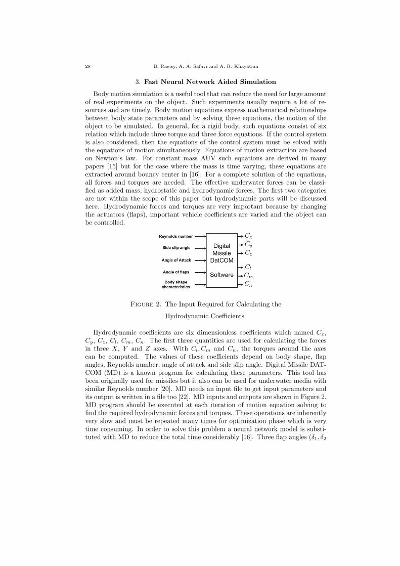
Body motion simulation is a useful tool that can reduce the need for large amountof real experiments on the object. Such experiments usually require a lot of re-sources and are timely. Body motion equations express mathematical relationshipsbetween body state parameters and by solving these equations, the motion of theobject to be simulated. In general, for a rigid body, such equations consist of sixrelation which include three torque and three force equations. If the control systemis also considered, then the equations of the control system must be solved withthe equations of motion simultaneously. Equations of motion extraction are basedon Newton’s law. For constant mass AUV such equations are derived in manypapers [15] but for the case where the mass is time varying, these equations areextracted around bouncy center in [16]. For a complete solution of the equations,all forces and torques are needed. The effective underwater forces can be classi-fied as added mass, hydrostatic and hydrodynamic forces. The first two categoriesare not within the scope of this paper but hydrodynamic parts will be discussedhere. Hydrodynamic forces and torques are very important because by changingthe actuators (flaps), important vehicle coefficients are varied and the object canbe controlled.
Figure 2. The Input Required for Calculating the
Hydrodynamic Coefficients
Hydrodynamic coefficients are six dimensionless coefficients which named Cx,Cy, Cz, Cl, Cm, Cn. The first three quantities are used for calculating the forcesin three X, Y and Z axes. With Cl, Cm and Cn, the torques around the axescan be computed. The values of these coefficients depend on body shape, flapangles, Reynolds number, angle of attack and side slip angle. Digital Missile DAT-COM (MD) is a known program for calculating these parameters. This tool hasbeen originally used for missiles but it also can be used for underwater media withsimilar Reynolds number [20]. MD needs an input file to get input parameters andits output is written in a file too [22]. MD inputs and outputs are shown in Figure 2.MD program should be executed at each iteration of motion equation solving tofind the required hydrodynamic forces and torques. These operations are inherentlyvery slow and must be repeated many times for optimization phase which is verytime consuming. In order to solve this problem a neural network model is substi-tuted with MD to reduce the total time considerably [16]. Three flap angles (δ1, δ2
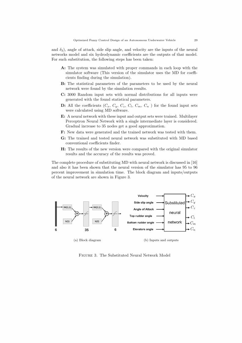
Optimized Fuzzy Control Design of an Autonomous Underwater Vehicle 29
and δ3), angle of attack, side slip angle, and velocity are the inputs of the neuralnetworks model and six hydrodynamic coefficients are the outputs of that model.For such substitution, the following steps has been taken:
A: The system was simulated with proper commands in each loop with thesimulator software (This version of the simulator uses the MD for coeffi-cients finding during the simulation).
B: The statistical parameters of the parameters to be used by the neuralnetwork were found by the simulation results.
C: 3000 Random input sets with normal distributions for all inputs weregenerated with the found statistical parameters.
D: All the coefficients (Cx, Cy, Cz, Cl, Cm, Cn ) for the found input setswere calculated using MD software.
E: A neural network with these input and output sets were trained. MultilayerPerceptron Neural Network with a single intermediate layer is considered.Gradual increase to 35 nodes get a good approximation.
F: New data were generated and the trained network was tested with them.
G: The trained and tested neural network was substituted with MD basedconventional coefficients finder.
H: The results of the new version were compared with the original simulatorresults and the accuracy of the results was proved.
The complete procedure of substituting MD with neural network is discussed in [16]and also it has been shown that the neural version of the simulator has 95 to 96percent improvement in simulation time. The block diagram and inputs/outputsof the neural network are shown in Figure 3.
IW{1,1}
b{1}
IW{2,1}
b{2}
+ +
6 35 6
(a) Block diagram (b) Inputs and outputs
Figure 3. The Substituted Neural Network Model
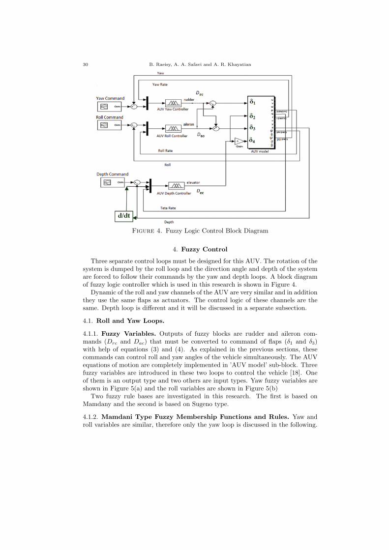
30 B. Raeisy, A. A. Safavi and A. R. Khayatian
tbh
Figure 4. Fuzzy Logic Control Block Diagram
4. Fuzzy Control
Three separate control loops must be designed for this AUV. The rotation of thesystem is dumped by the roll loop and the direction angle and depth of the systemare forced to follow their commands by the yaw and depth loops. A block diagramof fuzzy logic controller which is used in this research is shown in Figure 4.
Dynamic of the roll and yaw channels of the AUV are very similar and in additionthey use the same flaps as actuators. The control logic of these channels are thesame. Depth loop is different and it will be discussed in a separate subsection.
4.1. Roll and Yaw Loops.
4.1.1. Fuzzy Variables. Outputs of fuzzy blocks are rudder and aileron com-mands (Drc and Dac) that must be converted to command of flaps (δ1 and δ3)with help of equations (3) and (4). As explained in the previous sections, thesecommands can control roll and yaw angles of the vehicle simultaneously. The AUVequations of motion are completely implemented in ’AUV model’ sub-block. Threefuzzy variables are introduced in these two loops to control the vehicle [18]. Oneof them is an output type and two others are input types. Yaw fuzzy variables areshown in Figure 5(a) and the roll variables are shown in Figure 5(b)
Two fuzzy rule bases are investigated in this research. The first is based onMamdany and the second is based on Sugeno type.
4.1.2. Mamdani Type Fuzzy Membership Functions and Rules. Yaw androll variables are similar, therefore only the yaw loop is discussed in the following.
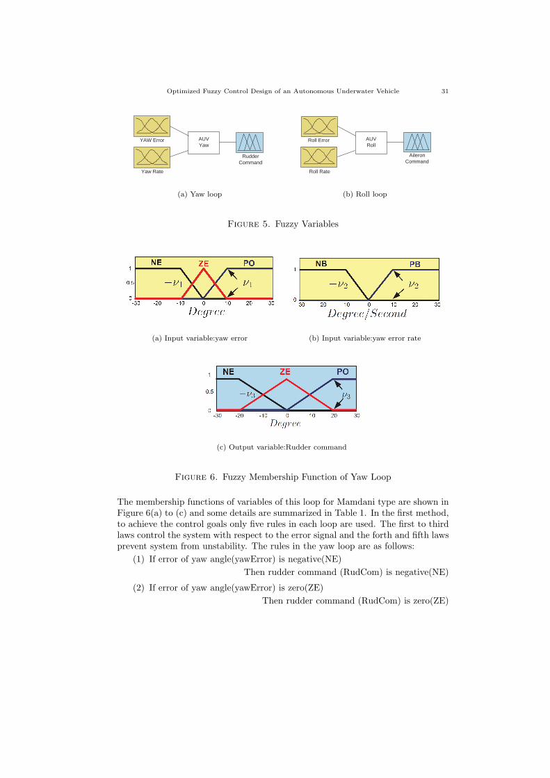
Optimized Fuzzy Control Design of an Autonomous Underwater Vehicle 31
AUV Yaw
YAW Error
Yaw Rate
Rudder Command
(a) Yaw loop
AUV Roll
Roll Error
Roll Rate
Aileron Command
(b) Roll loop
Figure 5. Fuzzy Variables
(a) Input variable:yaw error (b) Input variable:yaw error rate
(c) Output variable:Rudder command
Figure 6. Fuzzy Membership Function of Yaw Loop
The membership functions of variables of this loop for Mamdani type are shown inFigure 6(a) to (c) and some details are summarized in Table 1. In the first method,to achieve the control goals only five rules in each loop are used. The first to thirdlaws control the system with respect to the error signal and the forth and fifth lawsprevent system from unstability. The rules in the yaw loop are as follows:
(1) If error of yaw angle(yawError) is negative(NE)
Then rudder command (RudCom) is negative(NE)
(2) If error of yaw angle(yawError) is zero(ZE)
Then rudder command (RudCom) is zero(ZE)

32 B. Raeisy, A. A. Safavi and A. R. Khayatian
(3) If error of yaw angle(yawError) is positive(PO)
Then rudder command (RudCom) is positive(PO)
(4) If the rate of yaw angle(yawRate) is positive big (PB)
Then the rudder command (RudCom) is negative(NE).
(5) If the rate of yaw angle (yawRate) is negative big(NB)
Then the rudder command (RudCom) is positive(PO).
These rules in the roll loop can be shown simply by the following expressions:
If (rollError) is (NE) =⇒ (ileCom) = (NE)If (rollError) is (ZE) =⇒ (ileCom) = (ZE)If (rollError) is (PO) =⇒ (ileCom) = (PO)If (rollRate) is (PB) =⇒ (ileCom) = (NE)If (rollRate) is (NB) =⇒ (ileCom) = (PO)
Variable NameIn/Outtype
Name AbbreviationFuzzy Membership
type
Yaw Error InNegativeZero
Positive
NEZEPO
TrampfTrimfTrampf
yaw Rate InNegative BigPositive Big
NBPB
TrampfTrampf
Rud Command OutNegativeZero
Positive
NEZEPO
TrampfTrimfTrampf
Table 1. Parameters of Yaw Loop Fuzzy Variables
4.1.3. Sugeno Type Fuzzy Rules. In this method, the number of variables aresimilar to Mamdani type and two input variables and one output variable existat each loop. Although the number of variables are the same but the error ratemembership functions have been changed. As it is shown in Figure 7, error ratevariables in yaw and roll loops have been assigned to positive(PO), negative(NE)and zero(ZE) membership functions . The following rules have been introduced tocover all of the input variable ranges and control the system:
(1) If (yawError) is (NE) AND (yawRate) is (NE) =⇒ (RudCom) = (-C1)(2) If (yawError) is (NE) AND (yawRate) is (ZE) =⇒ (RudCom) = (-C2)(3) If (yawError) is (NE) AND (yawRate) is (PO) =⇒ (RudCom) = (-C3)(4) If (yawError) is (ZE) AND (yawRate) is (NE) =⇒ (RudCom) = (-C4)(5) If (yawError) is (ZE) AND (yawRate) is (ZE) =⇒ (RudCom) = 0(6) If (yawError) is (ZE) AND (yawRate) is (PO) =⇒ (RudCom) = (+C4)(7) If (yawError) is (PO) AND (yawRate) is (NE) =⇒ (RudCom) = (+C3)(8) If (yawError) is (PO) AND (yawRate) is (ZE) =⇒ (RudCom) = (+C2)
Optimized Fuzzy Control Design of an Autonomous Underwater Vehicle 33
(9) If (yawError) is (PO) AND (yawRate) is (PO) =⇒ (RudCom) = (+C1)
C1 to C4 are constants that they must be tunned to reach proper performance.Four pairs of laws are symmetric and then the value of outputs are chosen negativeof each other respectively.
Figure 7. Sugeno Method Yaw Error Rate Membership Function
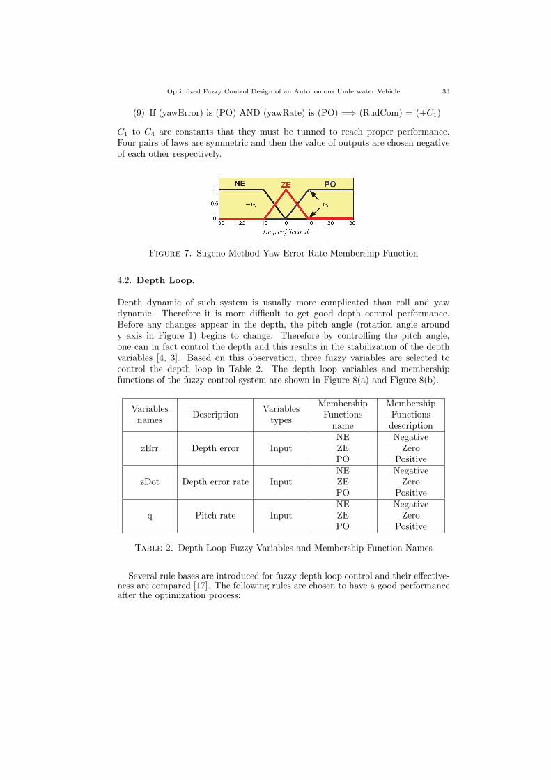
4.2. Depth Loop.
Depth dynamic of such system is usually more complicated than roll and yawdynamic. Therefore it is more difficult to get good depth control performance.Before any changes appear in the depth, the pitch angle (rotation angle aroundy axis in Figure 1) begins to change. Therefore by controlling the pitch angle,one can in fact control the depth and this results in the stabilization of the depthvariables [4, 3]. Based on this observation, three fuzzy variables are selected tocontrol the depth loop in Table 2. The depth loop variables and membershipfunctions of the fuzzy control system are shown in Figure 8(a) and Figure 8(b).
Variablesnames
DescriptionVariablestypes
MembershipFunctionsname
MembershipFunctionsdescription
zErr Depth error InputNEZEPO
NegativeZero
Positive
zDot Depth error rate InputNEZEPO
NegativeZero
Positive
q Pitch rate InputNEZEPO
NegativeZero
Positive
Table 2. Depth Loop Fuzzy Variables and Membership Function Names
Several rule bases are introduced for fuzzy depth loop control and their effective-ness are compared [17]. The following rules are chosen to have a good performanceafter the optimization process:
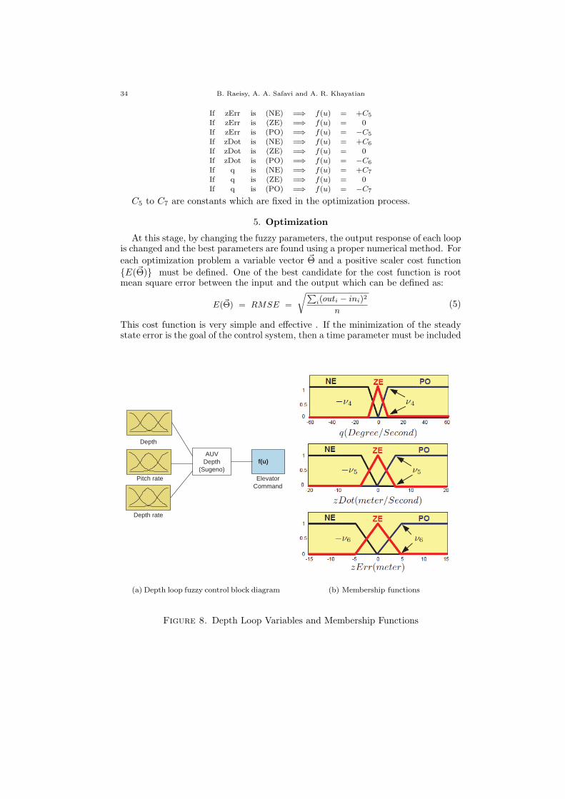
34 B. Raeisy, A. A. Safavi and A. R. Khayatian
If zErr is (NE) =⇒ f(u) = +C5
If zErr is (ZE) =⇒ f(u) = 0If zErr is (PO) =⇒ f(u) = −C5
If zDot is (NE) =⇒ f(u) = +C6
If zDot is (ZE) =⇒ f(u) = 0
If zDot is (PO) =⇒ f(u) = −C6
If q is (NE) =⇒ f(u) = +C7
If q is (ZE) =⇒ f(u) = 0If q is (PO) =⇒ f(u) = −C7
C5 to C7 are constants which are fixed in the optimization process.
5. Optimization
At this stage, by changing the fuzzy parameters, the output response of each loopis changed and the best parameters are found using a proper numerical method. For
each optimization problem a variable vector Θ⃗ and a positive scaler cost function
{E(Θ⃗)} must be defined. One of the best candidate for the cost function is rootmean square error between the input and the output which can be defined as:
E(Θ⃗) = RMSE =
√∑i(outi − ini)2
n(5)
This cost function is very simple and effective . If the minimization of the steadystate error is the goal of the control system, then a time parameter must be included
AUV Depth
(Sugeno)
Roll Error
Pitch rate Elevator Command
Depth rate
f(u)
Depth
(a) Depth loop fuzzy control block diagram (b) Membership functions
Figure 8. Depth Loop Variables and Membership Functions
Optimized Fuzzy Control Design of an Autonomous Underwater Vehicle 35
in the cost and this suggests the Integral Time Square Error(ITSE) for a betterperformance:
E(Θ⃗) = ITSE =∑i
ti × (outi − ini)2
(6)
In the depth and yaw loops, input commands are defined as step and all initialconditions are set to zero. In the roll loop, input command must be set to zerobut the initial condition is set to a nonzero value. In this research the normalizedsteepest descent method [8] was used as the optimization method.
The following notations are used to describe the optimization procedure:
Θ⃗ n dimensional vector of the parameters. n Number of parameters.
θi The ith parameters. m Step number.
E(Θ⃗) Cost function. g(Θ⃗) Gradient vector.
Θ⃗m Parameter vector in the mth iteration. κ(m) Variable step
Θ⃗ = [θ1 θ2 ... θn]T
(7)
g⃗(Θ⃗) = ▽(E(Θ⃗)) =dE(Θ⃗)
dΘ⃗ (8)
dE(Θ⃗)
dΘ⃗= [
∂E(Θ⃗)
∂θ1
∂E(Θ⃗)
∂θ2...∂(Θ⃗)
∂θn]T (9)
Θ⃗m+1 = Θ⃗m − κ(m)g⃗(Θ⃗)
∥g⃗(Θ⃗)∥ (10)
Although E(Θ⃗) is not usually an analytic function, but the gradient operator inequation 8 can be defined for non analytic functions too [9, 10]. For such functionsthe gradient must be estimated numerically.
Optimizing method begins by selecting an initial vector of parameters. In the rolland yaw loops, three methods are considered. In the first method, the optimizationalgorithm is applied to Mamdani fuzzy rule base and only the ν1 is allowed tobe changed (The knee of the PB and negative of the knee of the NB membershipfunction as shown in Figure 6(a)). In the second method ν1, ν2 and ν3 are allowed tovary (These variables are the knees of the membership function as shown in Figure6(a)-(c). In the third method, optimization algorithm is applied to the Sugeno rulebase parameters ν1, ν2 and C1, C2, C3 and C4, which were introduced in section4.1.3. The parameters of three optimization methods are summarized in Table 3.
In the depth loop, only one set of parameters are selected for optimization pro-cedure. These parameters are ν4, ν5 and ν6 in Figure 8(b) and C5, C6 and C7 whichwere introduced in section 4.2:
Θ⃗ = [ν4 ν5 ν6 C5 C6 C7]T
(11)

36 B. Raeisy, A. A. Safavi and A. R. Khayatian
First MethodMamdani with one variable
Θ⃗ = [ν1]T
Second MethodMamdani with three variables
Θ⃗ = [ν1 ν2 ν3]T
Third MethodSugeno with six variables
Θ⃗ = [ν1 ν2 C1 C2 C3 C4]T
Table 3. Vector of Variables in Three Optimization Methods
Vector of parameters must be updated at each iteration. The recursive equation(10) expresses the updating algorithm. Gradient vector in equation (9) is calculated
from partial derivative E(Θ⃗) versus θi in n step at each iteration. In order tocalculate the gradient vector, the input command is applied to the system simulator
and the response of the system is obtained. Then, the defined cost function E(Θ⃗)
is calculated. With the replacement of θi +∆θi with θi in the parameter vector(Θ⃗)the output is found again and the cost function is recalculated. Variation of thecost function versus the variation of θi shows the desired partial derivative. Toachieve a better performance, κ(m) is varied . At the first step, κ(1) is set to 1. If
E(Θ⃗) value decreases in two successive iterations κ(m) will be increased by 10%,
otherwise if E(Θ⃗) value increases, the program decreases κ(m) by 10% for the nextstep to get finer pacing.
6. Simulation Results
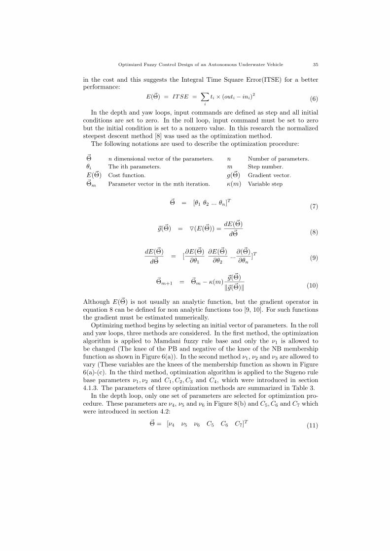
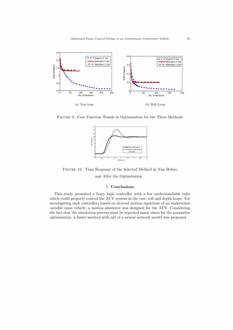
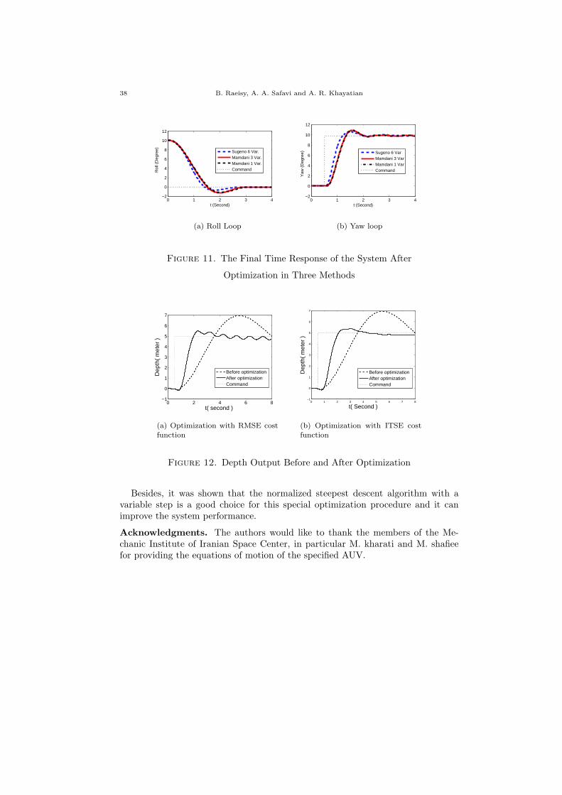
In this section, the results of simulations are discussed. The trends of the costfunction variation during the optimization procedure in all three methods in theyaw and roll loop are shown in Figures 9(b) and 9(a). These curves show that theSugeno method has better performance than the two other methods in both loops.Figure 10 shows how the optimization algorithm improves the yaw loop transientresponse. Figures 11(a) and 11(b) compares the final time response of the systemafter optimization process for different three methods. In both loops, optimizedSugeno method has a better performance not only in the peak overshoot but alsofor the rise time characteristics.
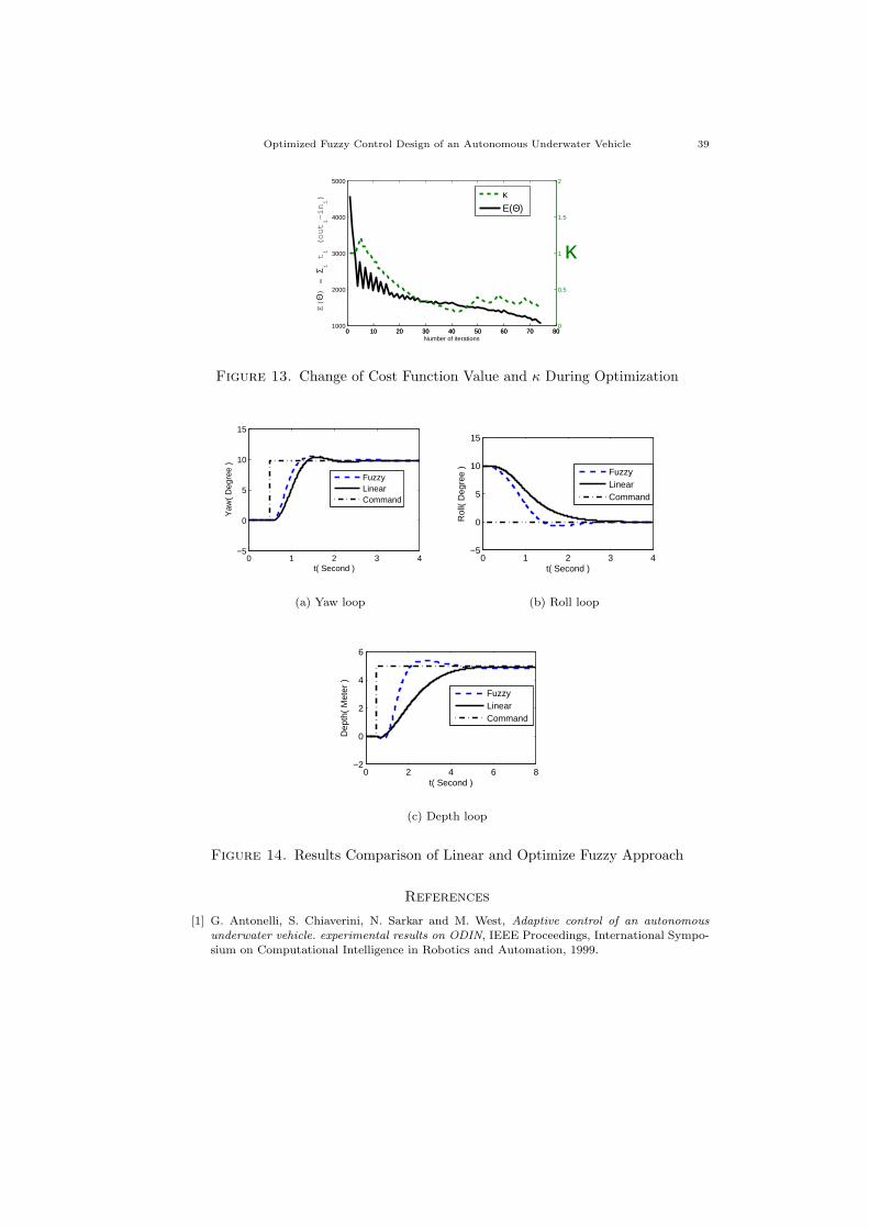
Depth loop simulation results are different from the two other loops. Figure 12(a)shows the output of the depth loop before and after optimization process with theRMSE criteria(equation (5)). As it can be seen there are some oscillations at theend of simulation time. Changing the cost function to ITSE criterion(equation (6)),the control performance at the end of simulation time is improved as it is shownin Figure 12(a). Figure 13 shows the behavior of the cost function and κ valuesduring the optimization process in the depth loop.
The results of optimized fuzzy method and linear approach [3] are compared inFigure 14. Figures 14(a) to 14(c) show the output of yaw, roll and depth loops forboth methods and all cases, the optimized fuzzy method has a better performancethan the linear method.
Optimized Fuzzy Control Design of an Autonomous Underwater Vehicle 37
0 50 100 150 200 2502.6
2.8
3
3.2
3.4
3.6
No. of iterations
E(Θ
) (D
egre
e)
Sugeno 6 VarMamdani 3 VarMamdani 1 Var
(a) Yaw loop
0 50 100 150 2004
4.2
4.4
4.6
4.8
E(Θ
) (D
egre
e)
No. of iterations
Sugeno 6 VarMamdani 3 VarMamdani 1 Var
(b) Roll Loop
Figure 9. Cost Function Trends in Optimization for the Three Methods
0 0.5 1 1.5 2 2.5 3 3.5 4−2
0
2
4
6
8
10
12
14
16
t( Second )
Yaw
( D
egre
e )
After optimizationBefore Optimizationcommand
Figure 10. Time Response of the Selected Method in Yaw Before
and After the Optimization
7. Conclusions
This study presented a fuzzy logic controller with a few understandable ruleswhich could properly control the AUV system in the yaw, roll and depth loops. Forinvestigating such controllers based on derived motion equations of an underwatervariable mass vehicle, a motion simulator was designed for the AUV. Consideringthe fact that the simulation process must be repeated many times for the parameteroptimization, a faster method with aid of a neural network model was proposed.
38 B. Raeisy, A. A. Safavi and A. R. Khayatian
0 1 2 3 4−2
0
2
4
6
8
10
12
t (Second)
Rol
l (D
egre
e)
Sugeno 6 Var.Mamdani 3 Var.Mamdani 1 Var.Command
(a) Roll Loop
0 1 2 3 4−2
0
2
4
6
8
10
12
t (Second)
Yaw
(D
egre
e)
Sugeno 6 VarMamdani 3 VarMamdani 1 VarCommand
(b) Yaw loop
Figure 11. The Final Time Response of the System After
Optimization in Three Methods
0 2 4 6 8−1
0
1
2
3
4
5
6
7
t( second )
Dep
th(
met
er )
Before optimizationAfter optimizationCommand
(a) Optimization with RMSE costfunction
0 1 2 3 4 5 6 7 8−1
0
1
2
3
4
5
6
7
t( Second )
Dep
th(
met
er )
Before optimizationAfter optimizationCommand
(b) Optimization with ITSE costfunction
Figure 12. Depth Output Before and After Optimization
Besides, it was shown that the normalized steepest descent algorithm with avariable step is a good choice for this special optimization procedure and it canimprove the system performance.
Acknowledgments. The authors would like to thank the members of the Me-chanic Institute of Iranian Space Center, in particular M. kharati and M. shafieefor providing the equations of motion of the specified AUV.
Optimized Fuzzy Control Design of an Autonomous Underwater Vehicle 39
0 10 20 30 40 50 60 70 801000
2000
3000
4000
5000
E(Θ
) =
Σ i
ti (
ou
ti−
ini)
Number of iterations
0 10 20 30 40 50 60 70 800
0.5
1
1.5
2
κE(Θ)
κ
Figure 13. Change of Cost Function Value and κ During Optimization
0 1 2 3 4−5
0
5
10
15
t( Second )
Yaw
( D
egre
e )
FuzzyLinearCommand
(a) Yaw loop
0 1 2 3 4−5
0
5
10
15
t( Second )
Rol
l( D
egre
e )
FuzzyLinearCommand
(b) Roll loop
0 2 4 6 8−2
0
2
4
6
t( Second )
Dep
th(
Met
er )
FuzzyLinearCommand
(c) Depth loop
Figure 14. Results Comparison of Linear and Optimize Fuzzy Approach
References
[1] G. Antonelli, S. Chiaverini, N. Sarkar and M. West, Adaptive control of an autonomousunderwater vehicle. experimental results on ODIN, IEEE Proceedings, International Sympo-sium on Computational Intelligence in Robotics and Automation, 1999.
40 B. Raeisy, A. A. Safavi and A. R. Khayatian
[2] A. Balasuriya and L. Cong, Adaptive fuzzy sliding mode controller for underwater vehicles,
IEEE Proceedings, The 4th international conference on control and automations (ICCA’03),Canada, June 2003.
[3] T. BinaZadeh, A. R. Khayatian and P. KarimAghaee, Identification and control of 6 DOF un-derwater variable mass object, 13th iranian conference on electrical engineering (ICEE2005),
Zanjan, Iran, 2005.[4] J. Blakelock, Automatic control of aircraft and missiles, 2nd edition, Willy, February 1991.[5] F. Dougherty, T. Sherman, G. Woolweaver and G. Lovell, An autonomous underwater ve-
hicle (AUV) flight control system using sliding mode control, Proceedings, OCEANS ’88.
Baltimore, MD USA, Oct. 1988.[6] T. Fossen and M. Blanke, Nonlinear output feedback control of underwater vehicle propellers
using feedback from estimated axial flow velocity, IEEE Journal of Oceanic Engineering, Apr2000.
[7] T. Fossen, Guidance and control of ocean vehicles, John Wiley & Sons, 1994.[8] J. S. Han, H. S. Kim and J. Neggers, Actions, norms, subactions and kernels of (fuzzy)
norms, Iranian Journal of Fuzzy Systems, 7(2) (2010), 141-147.[9] A. Hasankhani, A. Nazari and M. Sahelis, Some properties of fuzzy hilbert spaces and norm
of operators, Iranian Journal of Fuzzy Systems, 7(3) (2010), 129-157.[10] K. Ishii and T. Ura, An adaptive neural-net controller system for an underwater vehicle,
Control Engineering Practice, Elsevierm, 8(2) (2000), 177-184.
[11] J. S. R. Jang, C. T. Sun and E. Mizutani, Neuro-fuzzy and soft computing, Prentic Hall,1997.
[12] N. E. Leonard and P. S. Krishnaprasad, Motion control of an autonomous underwater vehiclewith an adaptive feature, IEEE Proceedings of Autonomous Underwater Vehicle Technology,
AUV ’94, Cambridge, MA, USA, Jul 1994.[13] J. H. Li, P. M. Lee and S. J. Lee, Neural net based nonlinear daptive control for autonomous
underwater vehicles, IEEE international Conference on Robotics and Automation, May 2002.[14] Y. Nakamura and S. Savant, Nonlinear tracking control of autonomous underwater vehicles,
IEEE Proceedings on Robotics and Automation, May 1992.[15] T. Prestero, Development of a six-degree of freedom simulation model for the REMUS au-
tonomous underwater vehicle, MTS/IEEE Conference and Exhibition, OCEANS, 2001.[16] B. Raeisy, M. Kharati, A. A. Safavi and A. R. Khayatian, Equation of motion derivation of
variable mass underwater vehicle and 6DOF simulation with helping of neural network, 17thAnual International Conference on Mechanical Engineering, Tehran, Iran, May 2009.
[17] B. Raeisy, A. A. Safavi and A. R. Khayatian, Fuzzy logic depth control of an autonomousunderwater vehicle and optimization of it with normalize steepened descent method, 17th
Anual International Conference on Mechanical Engineering, Tehran, Iran, May 2009.[18] B. Raeisy, A. A. Safavi and A. R. Khayatian, Optimized fuzzy logic yaw and roll control of
an autonomous underwater vehicle, 8th Iranian Conference on Fuzzy System, Tehran, Iran,
October 2008.[19] L. Rodrigues and P.Tavares, Sliding mode control of an AUV in the diving and steering
planes, MTS/IEEE Conference Proceedings, MG de Sousa Prado- OCEANS’96, Sep 1996.[20] N. Sey’edi and M. A. Mirjalili, Hydrodynamic stability coefficients calculation of submarine
and its weapons using added mass and misile DATCOM, 4th Conference of UnderwaterScience and Technology (fcoust), Isfahan, May 2007.
[21] E. Shivanian and E. Khoram, Optimization of linear objective function subject to fuzzy rela-tion inequalities constraints with max-product compozition, Iranian Journal of Fuzzy Systems,
7(3) (2010), 51-71.[22] S. R.Vukelich, S. L. Stoy and M. E. Moore, Missile DATCOM user’s manual, Dought Aircraft
Company Inc., 1988.[23] J. Wang and G. Lee, Self-adaptive recurrent neuro-fuzzy control of an autonomous underwa-
ter vehicle, IEEE Transactions on Robotics and Automation, 19(2) (2003).
Optimized Fuzzy Control Design of an Autonomous Underwater Vehicle 41
Behrooz Raeisy ∗, School of Electrical and Computer Engineering, Shiraz Univer-
sity, Shiraz, Iran and Iranian Space Agency, Iranian Space Center, Mechanic Institute,Shiraz, Iran, P.O. Box: 71555-414
E-mail address: [email protected]
Ali Akbar Safavi, School of Electrical and Computer Engineering, Shiraz Univer-sity, Shiraz, Iran
E-mail address: [email protected]
Ali Reza Khayatian, School of Electrical and Computer Engineering, Shiraz Uni-versity, Shiraz, Iran
E-mail address: [email protected]
*Corresponding author