Optimizing Energy Consumption of Data Flow in Mobile Ad Hoc

Optimizing Energy Consumption of Data Flow in Mobile Ad Hoc Wireless Networks1

HAIYANG HU HUA HU

College of Computer Science and Information Engineering, Zhejiang Gongshang University Hangzhou City, Zhejiang Province, CHINA, 310018

State Key Laboratory for Novel Software Technology, Nanjing University Jiangsu, Nanjing , CHINA, 210093

[email protected] Abstract: Because of the limited node battery power, energy optimization is important for the mobile nodes in wireless ad hoc networks. Controlled node mobility is an effective approach to reduce the communication energy consumption while the movement itself also consumes energy. Based on cooperative communication (CC) model, this paper takes the energy consumption of node movement and their individual residual energy into account, and then proposes localized algorithms for directing mobile node mobility and adapting their transmission power dynamically in mobile ad hoc networks. Compared with other algorithms by simulation, our mechanism named DEEF shows its efficiency in improving the system lifetime. Key-Words: ad hoc networks; node mobility; cooperative communication; energy consumption; multi-flow; local algorithm

1 Supported by NSFC (No. 60873022) and the open fund provided by State Key Laboratory for Novel Software Technology, Nanjing University

1 Introduction Ad hoc wireless networks consist of multiple wireless nodes that can communicate with each other by sending data flows either directly or through intermediate relays in the absence of a fixed infrastructure. The network topology, and specifically, the paths of flows, significantly affects communication energy efficiency at individual nodes. Being battery powered, these wireless nodes have limited operational time. Disproportionate energy consumption among them can lead to failure of the network. Recently, the optimization of the energy utilization of wireless nodes has received significant attention [9], [20], [21]. Different energy optimi-zation techniques including clustering [1], node mobility[12] and topology control [2], [3], [4] have been proposed.

In this paper, we use the approach of controlled node mobility to reduce the energy consumption of data flows in the mobile ad hoc network. We also take advantage of cooperative communication (CC) models to direct the nodes’ movement. By an effective incorporation of the node mobility and CC

model, we present a distributed energy-efficient flow scheme named DEEF to support data transmission in flow paths with less transmission power, and each mobile node are enable to make local decision on their controlled mobility. The remainder of this paper is organized as follows: In Section 2, we overview the related works. Section 3 describes the energy model and CC model. Problem description is also given in this section. In section 4, we analyze the controlled mobility optimization problem under CC model and discuss DEEF in detail that make controlled mobility decisions at individual nodes to maximize the system life. Section 5 presents the simulation results for DEEF and other algorithms, and section 6 concludes this paper. 2. Related Works In ad hoc wireless networks, mobile nodes can optimize their energy management by the approach of mobility. With predicting node movement, this kind of strategy has been used for topology control

WSEAS TRANSACTIONS on COMPUTERS

Haiyang Hu, Hua Hu and Yi Zhuang

ISSN: 1109-2750 977 Issue 7, Volume 7, July 2008

[6], energy optimization [7], and network throughput improvement [8]. In these approaches, the mobile nodes change their locations to optimize their transmission power and reducing energy consumption at other nodes. This controlled mobility strategy has been used widely as a means to reduce total energy consumption [10], [14], [15], [22], recover a disconnected topology [9], and increase sensor surveillance coverage [11], [12].

There are a lot of works discussing this controlled mobility. In [9], the authors proposed an approach that uses controlled mobility to improve communication reliability, specifically, to reconnect a partitioned mobile ad hoc network. In [11], [12], the authors presented localized algorithms that increase sensor surveillance coverage by distributing mobile sensor nodes to new locations where there were no other sensor nodes. In addition to the above research, other research activities on controlled mobility in sensor networks are reported in [18].

In [5], the authors consider energy consumption for both communication and mobility, then present global algorithm and localized algorithm to maximize the lifetime of flow and minimize the energy consumption. They incorporate the cost-benefit trade-off in the design of mobility strategies to optimize energy consumption.

In [10], the authors proposed several approaches that adjust the network topology to reduce energy consumption for the application of data flow. The approaches are based on the observation that total energy consumption is minimized when all relaying nodes are evenly spaced on a straight line between the source and the destination.

In [2], the authors address the topology control with cooperative communication (CC) problem in ad hoc wireless network. The model allows combining partial messages to decode a complete message. The objective of the [2] is to obtain a strongly-connected topology with minimum total energy consumption. Two distributed and localized algorithms are presented in [2] to be used by the nodes to set up their transmission power. Both algorithms can be applied on top of any symmetric, strongly-connected topology to reduce total power consumption.

Based on the above works, to optimize nodes’ energy consumption and maximize the lifetime of the system, this paper present a new localized mechanism named DEEF for data transmission in mobile ad hoc networks. It uses CC model among the mobile nodes, take the energy consumption of nodes’ mobility and their residual energy into account, and then proposes localized algorithms to

direct mobile node mobility and adapt their transmission power dynamically. Compared with other algorithms, our work shows its efficiency. 3. Problem Formulation In this section, we introduce the energy models for wireless communication, and CC model in this paper. Problem description is also given in this section. 3.1 Energy Models We adopt a transmission power model similar to the one used in [10] and [5]. In this model, the power for successful wireless data transmission is determined by the distance among the nodes and the noise level of their communication channel. Let

be the power needed for data transmission across distance d, then

)(dP

(1) αbdadP +=)(

Here，a, b, and α are constants dependent on the characteristics of the communication channel. The value of α is usually greater than or equal to 2. The energy consumption for transmitting l data bits across distance d is

)()( dPldETra ⋅= (2) In addition to transmission energy consumption,

we also consider the energy consumption for node mobility. Of course, mobility cost is dependent on the actual trace of node movement. For simplicity, we adopt a distance proportional cost model similar to the one used in [10]. In this model, the mobility cost can be calculated from the distance traversed,

)(dEMob

(3) dkdE mMob =)(

Here, is a constant dependent on the environment and the mass of the mobile node. For simplicity, we don’t take mobile node’s energy consumption for receiving data into account.

mk

3.2 Cooperative Communication Model In this paper, we take advantage of cooperative communication (CC) models that allows combining partial signals containing the same information to obtain the complete data. The CC model, has been introduced in [2], [11], and [19], in which transmitting independent copies of the signal from different locations results in having the receiver obtain independently faded versions of the signal, thus reducing the fading effect through multi-path propagation. In this communication model, each

WSEAS TRANSACTIONS on COMPUTERS Haiyang Hu, Hua Hu and Yi Zhuang


wireless node is assumed to transmit data and to act as a cooperative role, relaying data from other users. There are three versions of CC techniques [11] as amplify-and-forward, decode-and-forward, and selection relaying. This paper use the decode-and-forward version, where a node makes the relaying decision based on the signal-to-noise ratio (SNR) of the signal received. This model takes advantage of the physical layer design that combines partial signals containing the same information to obtain complete information.

The same to [2], [19], in this paper the message transmitted between nodes is encapsulated into a packet, which contains a preamble, a header, and a payload. A preamble is a sequence of predefined uncoded symbols assigned to facilitate timing acquisition, a header contains the error-control coded information sequence about the source/destination address and other control flags, and a payload contains the error-control coded message sequence.

There are two parameters related with SNR: pθ and cqαθ . pθ denotes the threshold needed to successfully decode the packet payload, and cqαθ denotes the threshold required for a successful time acquisition. We use k to denote the ratio of these two thresholds, pacqk θθ /= . We assume that the threshold to successfully decode a header is less than or equal to the threshold to successful time acquisition. A packet received with a SNR θ is: 1) fully received, if θθ ≤p , 2) partially received, if

pacq θθθ ≤≤

acq

, and 3) unsuccessfully received, if θθ < . Therefore, when a packet is fully or

partially received ( θθ ≤acq ), the header information is successfully decoded. In this paper, without losing generality, we only consider the case when

1=pθ , thus k acqpacq θθθ =/= . In the Ad hoc network using CC model, if node

i has set its transmission power level , where =ipow α

ibra + α is a communication medium dependent parameter, ri is the communication range of node i. And is denoted as the Euclidean distance between the nodes i and j, then the coverage provided by node i to node j is defined as: 1) = 1, if pow ; 2)

= , if ; 3) = 0, if pow . In CC model, the fully

received packet is defined as follows: suppose node j has m different neighbours; now, considering a transmission from node i to node j, if

, then node j is partially covered by i (or fully covered by i, if

). If combining all the packets partially or fully received from the different neighbors results in a full coverage of node j, i.e.

ijd

+ bda

+ bda

ijcov

)αijbd

ijd α </

1)/( ≥αiji

1)/( <≤ αijipowijcov

ijcov

/(i apow +

i

θacq

acqθ

1)/( <+≤ αθ ijiacq bdapow

1)/( ≥+ αiji bdapow

1)/( ≥+∑m mjm bdapow α , then for node j, the packet is fully received. 3.3 Problem Description We assume in ad hoc wireless network, the nodes are equipped with omni-directional antennas, and they are capable of receiving and combining partial received packets in accordance with the CC model.

For a flow composed of multiple nodes, we assume that the source and destination nodes of it are stationary, and other nodes are free to move to their new locations. The assumptions about energy consumption are made as follows:

Nodes are energy constrained with battery-driven, and they are mobile except the source and destination nodes of a flow.

Node movement consumes its energy. Nodes’ transmission power are tunable. They can select a transmission power level close to a specified value and use this power level for transmission.

Nodes can measure their residual node energy and detect their locations equipped with GPS or other position devices

Nodes can move to location specified by software applications and protocols.

Nodes can measure (or estimate from historical data) the energy needed to move to a target location, and they can determine the minimum transmission power needed to communicate with nodes within a specific distance.

4. Informed Mobility Using Cooper-ative Communication This paper presents an adaptive mechanism named DEEF based on node mobility and CC model in wireless ad hoc networks to maximize the system lifetime. In our approach, the flow node disseminates mobility strategy and status to other nodes along the flow path using message header of data packets. This scheme ensures that the mobility is naturally synchronized without additional synchronization overhead. Under the idea of CC, mobile nodes exchange information of their residual energy and current locations with their neighbours on the flow path to decide their next optimal



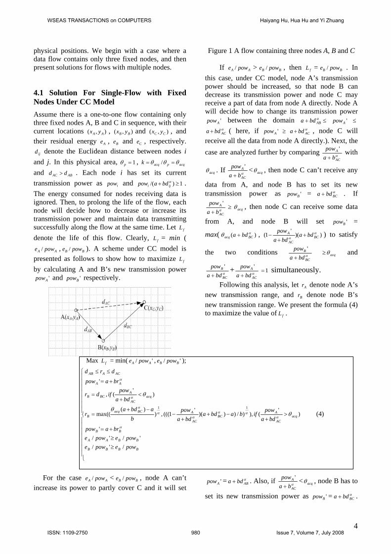
Figure 1 A flow containing three nodes A, B and C physical positions. We begin with a case where a data flow contains only three fixed nodes, and then present solutions for flows with multiple nodes.

If > , then = . In

this case, under CC model, node A’s transmission power should be increased, so that node B can decrease its transmission power and node C may receive a part of data from node A directly. Node A will decide how to change its transmission power

between the domain a

AA powe / BB powe / fL

+ bd

BB powe /

≤αAB Apow'Apow ' ≤

( here, if , node C will receive all the data from node A directly.). Next, the case are analyzed further by comparing

αACbda + 'Apow ≥ α

ACbda +

αAC

A

bapow+

' with

acqθ . If αAC

A

bapow+

' < acqθ , then node C can’t receive any

data from A, and node B has to set its new transmission power as = . If 'B bda +pow α

BC

αAC

A

bapow+

'≥ acqθ , then node C can receive some data

from A, and node B will set =

max( ,

'Bpow

)( αBCacq bda +θ )α

BCa)('

αAC

1(a

pow+

− A

bdbd+ ) to satisfy

the two conditions αBC

B 'bd

powa + acqθ≥ and

αB

bdapow+ BC

' + αAC

A 'bda

pow+

1= simultaneously.

4.1 Solution For Single-Flow with Fixed Nodes Under CC Model Assume there is a one-to-one flow containing only three fixed nodes A, B and C in sequence, with their current locations , and , and their residual energy , and , respectively.

denote the Euclidean distance between nodes i and j. In this physical area,

),( AA yx

Ae

),( BB yx

Be

1=p

),( CC yx

Ce

ijd

θ , acqpacqk θθθ == /

/( + αiji bda

fL

and . Each node i has set its current transmission power as and . The energy consumed for nodes receiving data is ignored. Then, to prolong the life of the flow, each node will decide how to decrease or increase its transmission power and maintain data transmitting successfully along the flow at the same time. Let denote the life of this flow. Clearly, = min (

, ). A scheme under CC model is presented as follows to show how to maximize by calculating A and B’s new transmission power

and respectively.

ABAC dd >

Apow Be /

'A pow

ipow 1) ≥

fL

fL

pow

Ae /

pow

Bpow

'BFollowing this analysis, let denote node A’s

new transmission range, and denote node B’s new transmission range. We present the formula (4) to maximize the value of .

Ar

Br

fL

Max = min( , ); fL '/ AA powe '/ BB powe

⎪⎪⎪⎪⎪⎪⎪

⎩

⎪⎪⎪⎪⎪⎪⎪

⎨

⎧

≥≥+=

>+

−++

−−+

=

<+

=

+=

≤≤

BBBB

BBAA

BB

acqAC

ABC

AC

ABCacqB

acqAC

ABCB

AA

ACAAB

powepowepowepowe

brapow

bdapow

ifbabdabda

powb

abdar

bdapow

ifdr

brapow

drd

/'/'/'/

'

)'

(),)/)))('

1(((,))(

max((

)'

(,

'

11

α

ααα

αα

α

α

α

θθ

θ

(4)

For the case < , node A can’t

increase its power to partly cover C and it will set = . Also, if AA powe / BB powe / 'Apow α

ABbda + αAC

A

bapow+

' < acqθ , node B has to

set its new transmission power as pow = . 'BαBCbda +

4



If αAC

A

bapow+

'≥ acqθ , node B will set =

max( ,

'Bpow

)αBC(θ acq a bd+ ))(

'1( α

α BCAC

A bdabda

pow+

+− ) to satisfy

the two conditions αBC

B

bdapow+

'acqθ≥ and

αBC

B

bdapow+

' + αAC

A

bdapow+

'1≥ . Following this analysis, we

present the formula (5) to maximize the value of fL

Max = min( , e ); fL 'A/A powe '/ BB pow

⎪⎪⎪⎪⎪⎪

⎩

⎪⎪⎪⎪⎪⎪

⎨

⎧

B

B

A

r

r

r

+=

>+

−++

−−+

=

<+

=

+=

=

α

ααα

αα

α

α

α

θθ

θ

BB

acqAC

ABC

AC

ABCacq

acqAC

ABC

AA

AB

brapow

bdapow

ifbabdabda

powb

abda

bdapow

ifd

brapow

d

'

)'

(),)/)))('

1(((,))(

max((

)'

(,

'

11

(5)

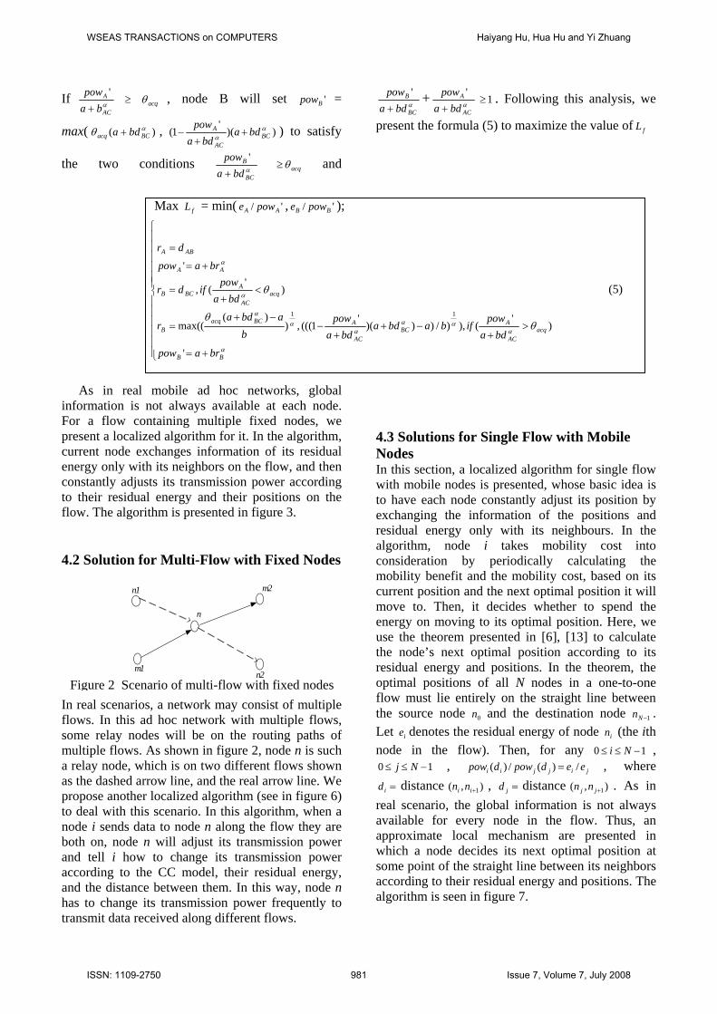
As in real mobile ad hoc networks, global

information is not always available at each node. For a flow containing multiple fixed nodes, we present a localized algorithm for it. In the algorithm, current node exchanges information of its residual energy only with its neighbors on the flow, and then constantly adjusts its transmission power according to their residual energy and their positions on the flow. The algorithm is presented in figure 3. 4.2 Solution for Multi-Flow with Fixed Nodes

m1

m2

n

n1

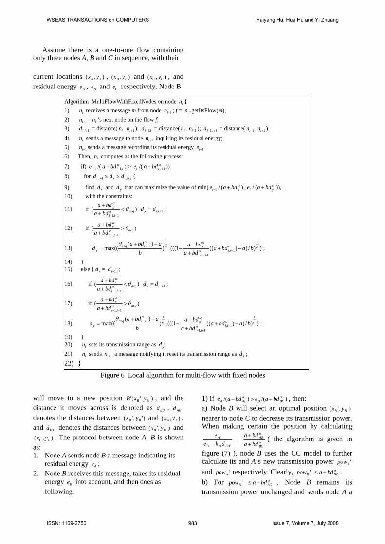
n2 In real scenarios, a network may consist of multiple flows. In this ad hoc network with multiple flows, some relay nodes will be on the routing paths of multiple flows. As shown in figure 2, node n is such a relay node, which is on two different flows shown as the dashed arrow line, and the real arrow line. We propose another localized algorithm (see in figure 6) to deal with this scenario. In this algorithm, when a node i sends data to node n along the flow they are both on, node n will adjust its transmission power and tell i how to change its transmission power according to the CC model, their residual energy, and the distance between them. In this way, node n has to change its transmission power frequently to transmit data received along different flows.

4.3 Solutions for Single Flow with Mobile Nodes In this section, a localized algorithm for single flow with mobile nodes is presented, whose basic idea is to have each node constantly adjust its position by exchanging the information of the positions and residual energy only with its neighbours. In the algorithm, node i takes mobility cost into consideration by periodically calculating the mobility benefit and the mobility cost, based on its current position and the next optimal position it will move to. Then, it decides whether to spend the energy on moving to its optimal position. Here, we use the theorem presented in [6], [13] to calculate the node’s next optimal position according to its residual energy and positions. In the theorem, the optimal positions of all N nodes in a one-to-one flow must lie entirely on the straight line between the source node and the destination node . Let denotes the residual energy of node (the ith node in the flow). Then, for any 0

0n 1−Nn

1ie in

−≤≤ Ni , 10 −≤≤ Nj , , where jijjii eedpowd /)(/)( =pow

=id distance , distance . As in real scenario, the global information is not always available for every node in the flow. Thus, an approximate local mechanism are presented in which a node decides its next optimal position at some point of the straight line between its neighbors according to their residual energy and positions. The algorithm is seen in figure 7.

)1+in, =jd ,( jn( in )1+jn

Figure 2 Scenario of multi-flow with fixed nodes



In this paper, we also take network topology constraint of connectivity into account. In our DEEF mechanism, mobile nodes move under the constraint that during the movement it should not move

outside of the transmission range of any of its current neighbours.

Alogorithm SingleFlowWithFixedNodes ( Flow f ) 1) For node in on the flow{ 2) 1+in is in ’s next neighbor on the flow; 2+in is 1+in ’s next neighbor on the flow; 3) Let 1, +iid be the Euclidean distance between in and 1+in ; 4) Let ie denote in ’s current residual energy; 5) ir denotes in ’s new power range, 6) Then, in computes as the following process: 7) if( ie /( α

1, ++ iibda ) > 1+ie /( α2,1 +++ iibda ))

8) for 2, +≤≤ iii dr { 1, +iid

9) find ir and 1+ir that can maximize the value of min( e / )αibra + , 1+ie / α

1( ++ ibra )) satisfying: i (

10) if )(2,

acqii

i θα < 2,11 +++ = iii dr ;

bdabra α

++

+

11) if )acqi θα

α

>

(

2,iibdabra

++

+

12) ))/) αba− ;

))(1(((,)

)(max((

1

2,12,

12,1

1α

α

αα

αθbda

bdabra

babda

r iiii

iiiacqi +

++

−−+

= +++

+++

13) } 14) else { ir = 1, +iid ;

15) if )(2,

acqii

i θα < 2,11 +++ = iii dr ;

bdabra α

++

+

16) if )acqi θα

α

>

(2,iibda

bra++

+

17) ))/) αba− ;

))(1(((,))(

max((1

2,12,

12,1

1α

α

αα

αθbda

bdabra

babda

r iiii

iiiacqi +

++

−−+

= +++

+++

18) } 19) in sets it’s transmission range as ir ; 20) in sends 1+in a message notifying it reset its transmission range as 1+ir ; 21) }

Figure 3 Localized algorithm for flows with fixed nodes

A C

B

r1 r2

B'

A C

B

B'

r1 r2

Figure 4 Node B moves to an optimal position nearer to node C Figure 5 Node B moves to an

optimal position further to node C



Assume there is a one-to-one flow containing only three nodes A, B and C in sequence, with their current locations , and , and residual energy , and respectively. Node B

),( AA yx

A Be

),( BB yx

Ce

),( CC yx

e

Algorithm MultiFlowWithFixedNodes on node in { 1) receives a message m from node ; f = .getItsFlow(m); in 1−in in2) 1+in = in ’s next node on the flow f; 3) 1, +iid = distance( in , 1+in ); iid ,1− = distance( in , 1−in ); 1,1 +− iid = distance( 1−in , 1+in );

4) in sends a message to node 1−in inquiring its residual energy; 5) 1−in sends a message recording its residual energy 1−ie 6) Then, in computes as the following process:

7) if( 1−ie /( αiibda ,1−+ ) > ie /( α

1, ++ iibda ))

8) for 2,1, ++ ≤≤ iixii ddd {

9) find xd and yd that can maximize the value of min( / ) , ie / αybda +( )), 1−ie ( α

xbda +10) with the constraints:

)(1,1

acqii

x

bdabda

θα

α

<++

+− will move to a new position , and the distance it moves across is denoted as . denotes the distances between and , and denotes the distances between ( and

. The protocol between node A, B is shown as:

)','(' BB yxB

)','( BB yx

Bx

'BBd

( Ax

',' By

'ABd

), Ay

CBd '

)Cy

)

,( Cx

1. Node A sends node B a message indicating its residual energy Ae ;

2. Node B receives this message, takes its residual energy Be into account, and then does as following:

1) If , then: )/()/( ααBCBABA bdaebdae +>+

a) Node B will select an optimal position nearer to node C to decrease its transmission power. When making certain the position by calculating

)','( BB yx

=− 'BBmB

A

dkee

α

α

BC

AB

bdabda

++ ( the algorithm is given in

figure (7) ), node B uses the CC model to further calculate its and A’s new transmission power and respectively. Clearly, .

'BpowαBCbd'Apow 'Bpow a +≤

b) For , Node B remains its transmission power unchanged and sends node A a

'Bpow αBCbda +≤

11) if ; 1, += iiy dd

)(1,1

acqii

x

bdabda θα

α

>++

+−

12) if

13) ))/)))(1(((,))(

max((1

1,1,1

11, αα

α

αα

αθbabda

bdabda

babda

d iiii

xiiacqy −+

++

−−+

= ++−

+ ;

14) } 15) else { xd = iid ,1− ;

16) if )(1,1

acqii

x

bdabda θα

α

<++

+−

1, += i ; iy dd

17) if )(1,1

acqii

x

bdabda θα

α

>++

+−

18) ))/)))(1(((,))(

max((1

1,1,1

11, αba− ; α

α

αα

αθbda

bdabda

babda

d iiii

xiiacqy +

++

−−+

= ++−

+

19) } 20) in sets its transmission range as yd ;

21) in sends 1+in a message notifying it reset its transmission range as xd ; 22) }

Figure 6 Local algorithm for multi-flow with fixed nodes



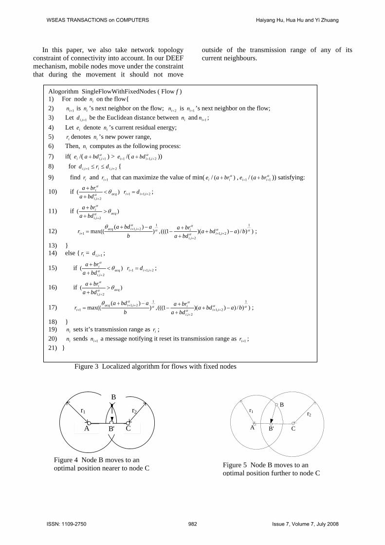
message indicating node A’s new transmission power; c) After receiving the message, node A sets its temporal transmission power

. It sends node B an ACK message;

=tApow

αα',max( ABAB bdabda ++ )', Apow

d) After receiving the message, node B begins to move to the next position; e) After arriving at the optimal position, node B sends node A a message notifying it to reset the power and sets the power of itself as

. =Apow

'Bpow

'Apow

=Bpow

The above process is presented in figure 4, where the r1 denotes A’s temporal transmission range with

the value ,,( 'ABAB ddMax ))/)'((1αbapowA − , and r2

denotes B’s temporal transmission range with the

value α1

)/)(( bapowB − . During node B’s movement, if it is always in the two circles at the same time, clearly, the topology constraint for connectivity will not be violated. 2) If , then: )/()/( αα

BCBABA bdaebdae +<+

a) Node B will select an optimal position farther to node C and nearer to node A to increase its transmission power and decreases node A’s power. After making certain the position by calculating

)','( BB yx

α

α

CB

AB

BBmB

A

bdabda

dkee

'

'

' ++

=−

, node B uses the CC model to

computing its and A’s new transmission power and respectively. Then node B sets its

temporal power as = , and begins to move.

'Bpow 'ApowtBpow

a +

αCBbda '+

αAB

b) During node B’s movement, node A remains its transmission power as ; bd

c) After arriving at the optimal position, node B sends node A a message notifying it to reset the power =A powpow 'A and sets the power of itself

=Bpow 'Bpow . The above process is presented in figure 5,

where the r1 denotes A’s temporal transmission

range with the value r1 = α1

)/)( powA − ba , and r2 denotes B’s temporal transmission range with the

value r2 = α1

)/)(( . Clearly, during node B’s movement, if it is always in the two circles at the same time, clearly, the topology constraint for connectivity will not be violated.

ba−powtB

1) void FindNextPosition(Node in ){ 2) 1−in is in ’s pre-neighbor on the flow; 3) 1+in is in ’s next-neighbor on the flow; 4) ),( 11 −− ii yx is 1−in ’s current position; 5) ),( 11 ++ ii yx is 1+in ’s current position; 6) for 11 ' +− << iBi xxx and 11 ' +− << iBi yyy {

7) if (11

1111

11

11 ''−+

+−+−

−+

−+

−−

+−−

==ii

iiiiB

ii

iiB xx

yxxyxxxyyy )

8) and (21

22 ))'()'(( BBBBmB

A

yyxxke

e

−+−− 221

21

221

21

))'()'((

))'()'((α

α

BiBi

iBiB

yyxxba

yyxxba

−+−+

−+−+==

++

−− )

9) in select its next position as )','( BB yx ; 10) }

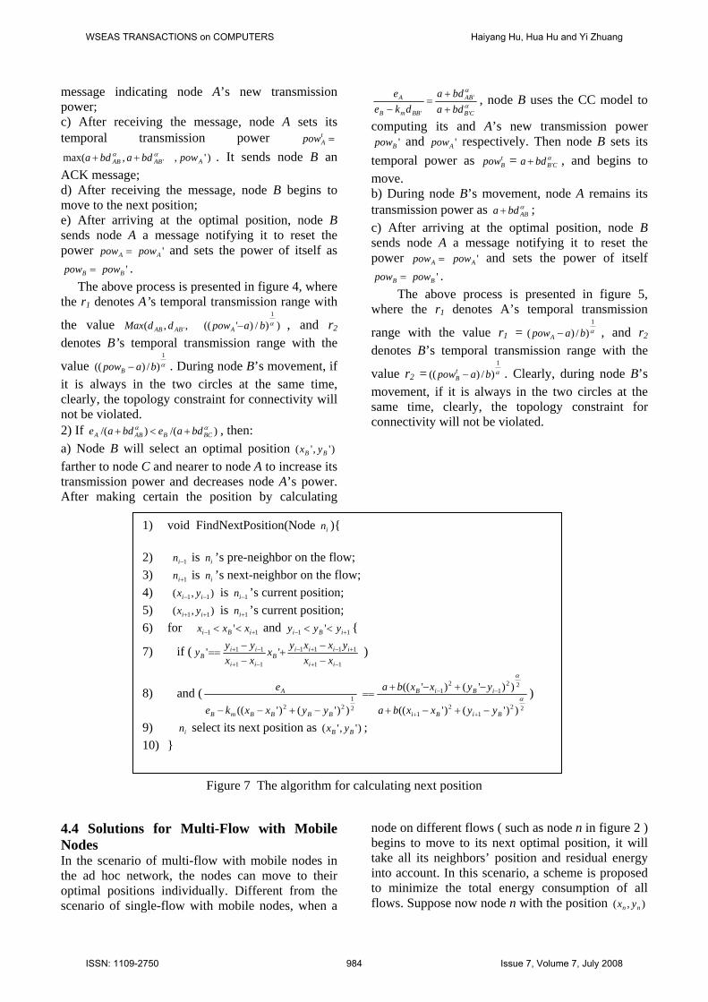
Figure 7 The algorithm for calculating next position 4.4 Solutions for Multi-Flow with Mobile Nodes In the scenario of multi-flow with mobile nodes in the ad hoc network, the nodes can move to their optimal positions individually. Different from the scenario of single-flow with mobile nodes, when a

node on different flows ( such as node n in figure 2 ) begins to move to its next optimal position, it will take all its neighbors’ position and residual energy into account. In this scenario, a scheme is proposed to minimize the total energy consumption of all flows. Suppose now node n with the position ),( nn yx



is on k different flows. On each flow , it has a preceding neighbour with the positions , and a succeeding neighbour with the positions

. Each flow has its traffic amount as . is denoted as the Euclidean distance between

node i and its succeeding neighbour j. Each node i has set its initial transmission power as

if

is

if

),(ii SS yx

iwiD

),(ii DD yx

ijd

=),( jip . When one neighbor sends the data to node n

along , node n sends it to the responding succeeding neighbor on . The total power

consumption is: + .

When

αijbda +

if

if

∑=

=k

iiitotal nSpwE

1),( ∑

=

k

iii Dnpw

1),(

0=∂∂

n

total

yE,0=

∂∂

n

total andx

E , the minimize value of

can be got. Thus, with totalE 2=α , the result is

and +

. By the analysis, a local

algorithm for multi-flow is given in figure 8.

∑∑ ∑== =

+k

ii

k

i

k

iDiSi wxwxw

ii11 1

2/)

)Di iy ∑

=

k

iiw

1

2/

=nx (

1∑=

k

i

w

=ny ∑=

k

iSi i

yw1

(

5. Simulation Results We set up a 100 area with mobile nodes distributed in randomly. We randomly select two nodes as the source and destination of the flow. The number of nodes the flow containing vary from three to ten. Evaluation of comparing DEEF with other algorithms presented in [2], [5], [6], and [19] are given for testing system lifetime under different mechanisms. The different parameters’ influences on the results under practical energy constraints are discussed in this section. The input parameters needed is listed in table 1 as follows:

mm 100×

Parameter Value

Net Size 100mX100m Node number in flow 10 a 50nJ/bit b 13pJ/bit/m2

α 2 Threshold distance( d0) 75m Flow length [0.5MB, 640MB] Packet header size 25 bytes Mobile node’s initial energy

[5J, 10J]

Threshold to decode the packet payload pθ

1

Threshold for time acquisition cqαθ

[0.1, 0.5]

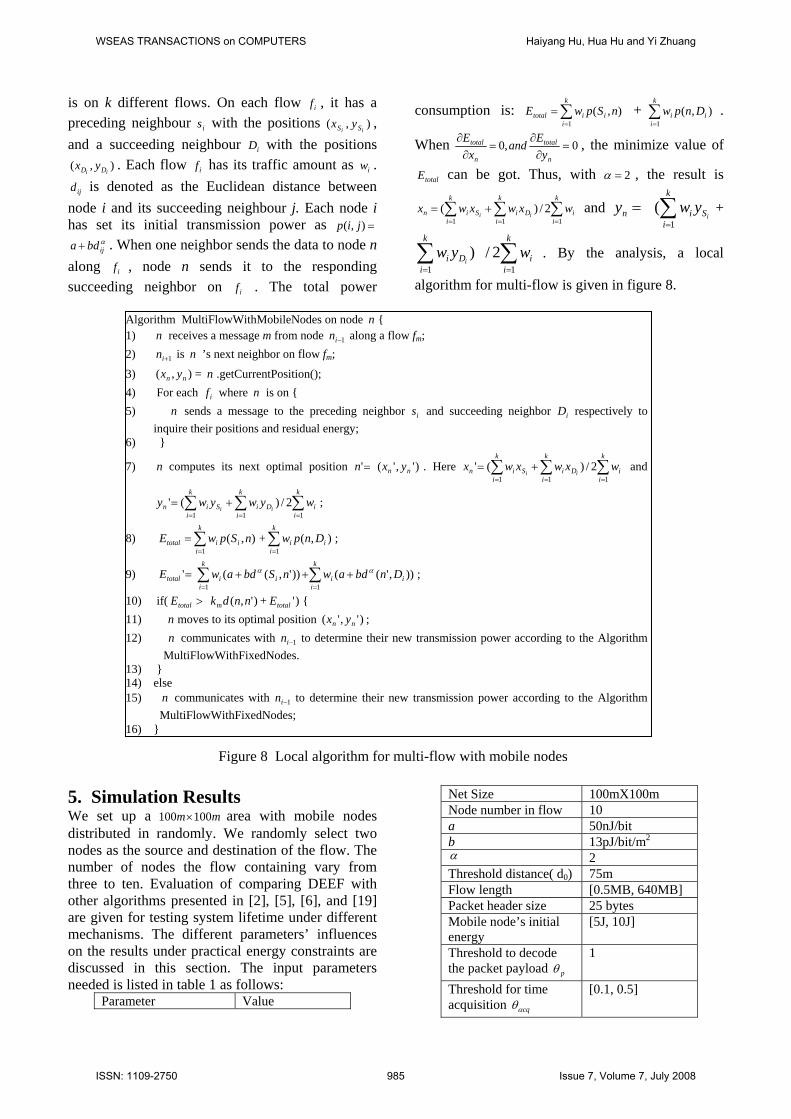
Algorithm MultiFlowWithMobileNodes on node n { 1) n receives a message m from node 1−in along a flow fm; 2) 1+in is n ’s next neighbor on flow fm;

3) ),( nn yx = n .getCurrentPosition(); 4) For each if where n is on { 5) n sends a message to the preceding neighbor is and succeeding neighbor iD respectively to

inquire their positions and residual energy; 6) }

7) n computes its next optimal position ='n

bdα

)','( nn yx . Here ∑k

xi

and

∑2/)

∑ ∑= =

k

iDin xw

1 12/)'

=iiw

1+=

k

iSi xw

i(

∑ ∑== =

+=k

i

k

iDSn yy

ii1

( iw' ;

Dn,

∑=

+k

i 1

k

i

=

=

i yw1 1

n

bd α

iw

∑=

k

i 1

∑=

k

i 1

8) ii Spw ),( + pw ( ; totalE ∑=

k

iii

1)

9) i'totalE ++ iii DnawnSaw ())',(( )),'( ;

10) if( >total )',( nndkm + )'totalE { E11) n moves to its optimal position )','( nn yx ; 12) n communicates with 1−in to determine their new transmission power according to the Algorithm

MultiFlowWithFixedNodes. 13) } 14) else 15) n communicates with 1−in to determine their new transmission power according to the Algorithm

MultiFlowWithFixedNodes; 16) }

Figure 8 Local algorithm for multi-flow with mobile nodes



Constant of mobility cost km

[0.1J, 1J]

Mobile node’s initial transmission range

20m

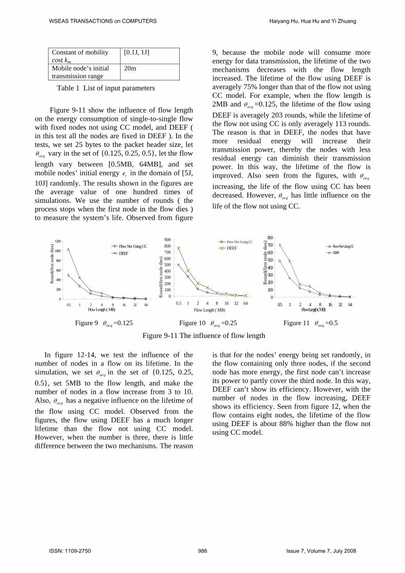
Figure 9-11 show the influence of flow length on the energy consumption of single-to-single flow with fixed nodes not using CC model, and DEEF ( in this test all the nodes are fixed in DEEF ). In the tests, we set 25 bytes to the packet header size, let

cqαθ vary in the set of {0.125, 0.25, 0.5}, let the flow length vary between [0.5MB, 64MB], and set mobile nodes’ initial energy in the domain of [5J, 10J] randomly. The results shown in the figures are the average value of one hundred times of simulations. We use the number of rounds ( the process stops when the first node in the flow dies ) to measure the system’s life. Observed from figure

9, because the mobile node will consume more energy for data transmission, the lifetime of the two mechanisms decreases with the flow length increased. The lifetime of the flow using DEEF is averagely 75% longer than that of the flow not using CC model. For example, when the flow length is 2MB and

ie

cqαθ =0.125, the lifetime of the flow using DEEF is averagely 203 rounds, while the lifetime of the flow not using CC is only averagely 113 rounds. The reason is that in DEEF, the nodes that have more residual energy will increase their transmission power, thereby the nodes with less residual energy can diminish their transmission power. In this way, the lifetime of the flow is improved. Also seen from the figures, with cqαθ increasing, the life of the flow using CC has been decreased. However, cqαθ has little influence on the life of the flow not using CC.

0

200

400

600

800

1000

1200

0.5 1 2 4 8 16 32 64

Flow Not Using CCDEEF

Flow Length ( MB)

Rou

nd(f

irst n

ode

dies

)

0100200300400500600700800900

0.5 1 2 4 8 16 32 64

Flow Not Using CC

DEEF

Rou

nd(fi

rst n

ode

dies

)

Flow Length ( MB)

0100200300400500600700800

0.5 1 2 4 8 16 32 64


Rou

nd(f

irst n

ode

dies

)

Flow Length ( MB)

Table 1 List of input parameters

Figure 9 cqαθ =0.125 Figure 10 cqαθ =0.25 Figure 11 cqαθ =0.5

Figure 9-11 The influence of flow length

In figure 12-14, we test the influence of the number of nodes in a flow on its lifetime. In the simulation, we set cqαθ in the set of {0.125, 0.25, 0.5}, set 5MB to the flow length, and make the number of nodes in a flow increase from 3 to 10. Also, cqαθ has a negative influence on the lifetime of the flow using CC model. Observed from the figures, the flow using DEEF has a much longer lifetime than the flow not using CC model. However, when the number is three, there is little difference between the two mechanisms. The reason

is that for the nodes’ energy being set randomly, in the flow containing only three nodes, if the second node has more energy, the first node can’t increase its power to partly cover the third node. In this way, DEEF can’t show its efficiency. However, with the number of nodes in the flow increasing, DEEF shows its efficiency. Seen from figure 12, when the flow contains eight nodes, the lifetime of the flow using DEEF is about 88% higher than the flow not using CC model.



10

30

50

70

90

110

130

3 4 5 6 7 8 9 10

Flow Not Using CC

DEEF

Rou

nd(f

irst n

ode

dies

Number of Node in Flow

0

20

40

60

80

100

120

3 4 5 6 7 8 9 10


Flow Length ( MB)

Rou

nd(f

irst n

ode

dies

)

0

20

40

60

80

100

120

3 4 5 6 7 8 9 10

DEEFFlow Not Using CC

Flow Length ( MB)

Rou

nd(f

irst n

ode

dies

)

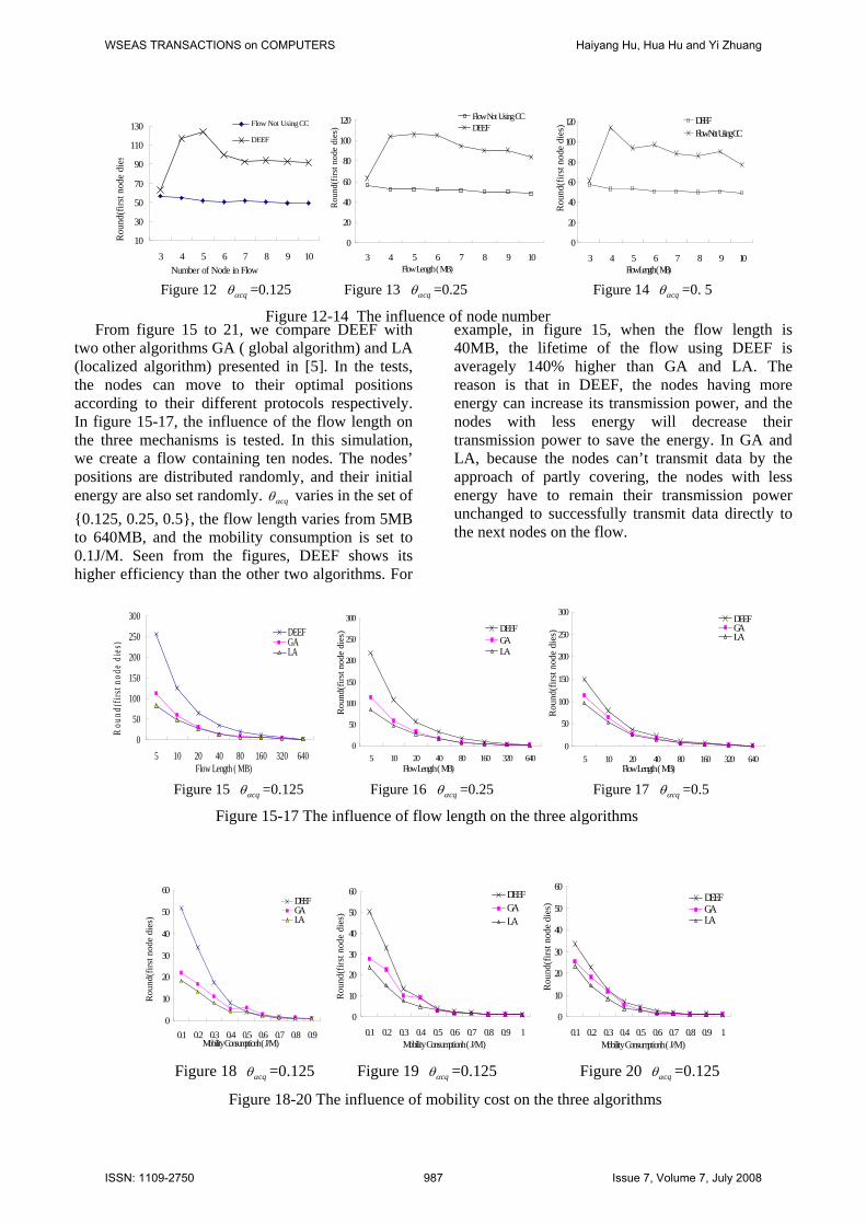
From figure 15 to 21, we compare DEEF with two other algorithms GA ( global algorithm) and LA (localized algorithm) presented in [5]. In the tests, the nodes can move to their optimal positions according to their different protocols respectively. In figure 15-17, the influence of the flow length on the three mechanisms is tested. In this simulation, we create a flow containing ten nodes. The nodes’ positions are distributed randomly, and their initial energy are also set randomly. cqαθ varies in the set of {0.125, 0.25, 0.5}, the flow length varies from 5MB to 640MB, and the mobility consumption is set to 0.1J/M. Seen from the figures, DEEF shows its higher efficiency than the other two algorithms. For

example, in figure 15, when the flow length is 40MB, the lifetime of the flow using DEEF is averagely 140% higher than GA and LA. The reason is that in DEEF, the nodes having more energy can increase its transmission power, and the nodes with less energy will decrease their transmission power to save the energy. In GA and LA, because the nodes can’t transmit data by the approach of partly covering, the nodes with less energy have to remain their transmission power unchanged to successfully transmit data directly to the next nodes on the flow.

0

50

100

150

200

250

300

5 10 20 40 80 160 320 640

DEEFGALA

Flow Length ( MB)

Rou

nd(fi

rst n

ode

dies

)

0

50

100

150

200

250

300

5 10 20 40 80 160 320 640

DEEFGALA

Flow Length ( MB)

Rou

nd(f

irst n

ode

dies

)

0

50

100

150

200

250

300

5 10 20 40 80 160 320 640

DEEFGALA

Flow Length ( MB)

Rou

nd(f

irst n

ode

dies

)

0

10

20

30

40

50

60

0.1 0.2 0.3 0.4 0.5 0.6 0.7 0.8 0.9

DEEFGALA

Mobility Consumptionh ( J/M )

Rou

nd(f

irst n

ode

dies

)

0

10

20

30

40

50

60

0.1 0.2 0.3 0.4 0.5 0.6 0.7 0.8 0.9 1

DEEFGALA

Rou

nd(f

irst n

ode

dies

)


0

10

20

30

40

50

60

0.1 0.2 0.3 0.4 0.5 0.6 0.7 0.8 0.9 1

DEEFGALA

Rou

nd(f

irst n

ode

dies

)


Figure 12 cqαθ =0.125 Figure 13 cqαθ =0.25 Figure 14 cqαθ =0. 5

Figure 12-14 The influence of node number

Figure 15 cqαθ =0.125 Figure 16 cqαθ =0.25 Figure 17 cqαθ =0.5 Figure 15-17 The influence of flow length on the three algorithms

Figure 18 cqαθ =0.125 Figure 19 cqαθ =0.125 Figure 20 cqαθ =0.125

Figure 18-20 The influence of mobility cost on the three algorithms



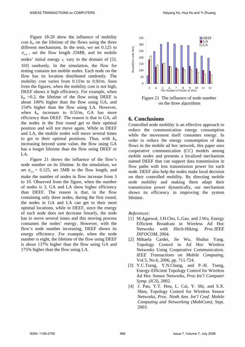
Figure 18-20 show the influence of mobility

cost km on the lifetime of the flows using the three different mechanisms. In the tests, we set 0.125 to

cqαθ , set the flow length 25MB, and let mobile nodes’ initial energy vary in the domain of [5J, 10J] randomly. In the simulation, the flow for testing contains ten mobile nodes. Each node on the flow has its location distributed randomly. The mobility cost varies from 0.1J/m to 0.9J/m. Seen from the figures, when the mobility cost is not high, DEEF shows it high efficiency. For example, when km =0.2, the lifetime of the flow using DEEF is about 100% higher than the flow using GA, and 154% higher than the flow using LA. However, when km increases to 0.5J/m, GA has more efficiency than DEEF. The reason is that in GA, all the nodes in the first round get to their optimal position and will not move again. While in DEEF and LA, the mobile nodes will move several times to get to their optimal positions. Thus, with km increasing beyond some value, the flow using GA has a longer lifetime than the flow using DEEF or LA.

ie

Figure 21 shows the influence of the flow’s node number on its lifetime. In the simulation, we set cqαθ = 0.125, set 5MB to the flow length, and make the number of nodes in flow increase from 3 to 10. Observed from the figure, when the number of nodes is 3, GA and LA show higher efficiency than DEEF. The reason is that, in the flow containing only three nodes, during the first round, the nodes in GA and LA can get to their most optimal locations, while in DEEF, since the energy of each node does not decrease linearly, the node has to move several times and this moving process consumes the nodes’ energy. However, with the flow’s node number increasing, DEEF shows its energy efficiency. For example, when the node number is eight, the lifetime of the flow using DEEF is about 137% higher than the flow using GA and 175% higher than the flow using LA.

0

50

100

150

200

250

300

350

3 4 5 6 7 8 9 10 11 12

DEEFGALA

The Number of Nodes in Flow

Rou

nd(f

irst n

ode

dies

)

Figure 21 The influence of node number

on the three algorithms

6. Conclusions Controlled node mobility is an effective approach to reduce the communication energy consumption while the movement itself consumes energy. In order to reduce the energy consumption of data flows in the mobile ad hoc network, this paper uses cooperative communication (CC) models among mobile nodes and presents a localized mechanism named DEEF that can support data transmission in flow paths with less transmission power for each node. DEEF also help the nodes make local decision on their controlled mobility. By directing mobile node mobility and making them adapt their transmission power dynamically, our mechanism shows its efficiency in improving the system lifetime. References: [1] M.Agarwal, J.H.Cho, L.Gao, and J.Wu, Energy

Efficient Broadcast in Wireless Ad Hoc Networks with Hitch-Hiking. Proc.IEEE INFOCOM, 2004.

[2] Mihaela Cardei, Jie Wu, Shuhui Yang. Topology Control in Ad Hoc Wireless Networks Using Cooperative Communication. IEEE Transactions on Mobile Computing, Vol.5, No.6, 2006, pp. 711-724.

[3] Y.C.Tseng, Y.N.Chang, and P.-H. Tseng, Energy-Efficient Topology Control for Wireless Ad Hoc Sensor Networks, Proc.Int’l Computer Symp. (ICS), 2002.

[4] J. Pan, Y.T. Hou, L. Cai, Y. Shi, and S.X. Shen, Topology Control for Wireless Sensor Networks, Proc. Ninth Ann. Int’l Conf. Mobile Computing and Networking (MobiCom), Sept. 2003.



[5] C.Tang, Philip.K.M, Energy Optimization under Informed Mobility. IEEE Trans. Parallel and Distributed Systems, Vol.17, No.9, 2006, pp.947-962.

[6] J. Wu and F. Dai, Mobility-Sensitive Topology Control in Mobile Ad Hoc Networks, Proc. Int’l Parallel and Distributed Processing Symp. (IPDPS), 2004.

[7] S. Chakraborty, D. Yau, and J. Lui. On the Effectiveness of Movement Prediction to Reduce Energy Consumption in Wireless Comm. (Extended Abstract), Proc. SIGMETRICS, June 2003.

[8] M.Grossglauser, D.Tse, Mobility Increases the Capacity of Ad-Hoc Wireless Networks, Proc. INFOCOM, pp. 1360-1369, Mar. 2000.

[9] S.Capkun, J.P.Hubaux,, L.Buttyan, Mobility Helps Security in Ad Hoc Networks, Proc. Fourth ACM Int’l Symp. Mobile Ad Hoc Networking and Computing (MobiHoc), June 2003

[10] D. Goldenberg, J. Lin, A.S. Morse, B. Rosen, Y.R. Yang, Towards Mobility as a Network Control Primitive, Proc. MobiHoc, 2004.

[11] N.Laneman, D.Tse, G.Wornell, Cooperative Diversity in Wireless Networks: Efficient Protocols and Outage Behavior, IEEE Trans. Information Theory, 2003.

[12] A.Chakrabarti, A.Sabharwal, B.Aazhang, Using Predictable Observer Mobility for Power Efficient Design of Sensor Networks, Information Processing in Sensor Networks, Apr. 2003.

[13] A.Nosratinia, T.E.Hunter, A.Hedayat, Cooperative Communication in Wireless Networks, IEEE Comm. Magazine, Vol.42, No.10, 2004, pp. 74-80.

[14] J.G. Proakis, Digital Communications, fourth ed. McGraw Hill, 2001.

[15] T.Srinidhi, G.Sridhar, V.Sridhar, Topology Management in Ad Hoc Mobile Wireless Networks, Proc. Real-Time Systems Symp, 2003.

[16] G.Wang, G.Cao, T.L.Porta, Movement-Assisted Sensor Deployment, Proc. IEEE INFOCOM, Mar. 2004.

[17] G.Wang, G.Cao, T.L.Porta, A Bidding Protocol for Deploying Mobile Sensors, Proc. IEEE Int’l Conf. Network Protocols (ICNP), Nov. 2003.

[18] P.Santi, D.M.Blough, F.Vainstein, A Probabilistic Analysis for the Range Assignment Problem in Ad Hoc Networks, Proc. ACM Mobihoc, pp. 212-220, Aug. 2000.

[19] J.Wu, M.Cardei, F.Dai, S.Yang, Extended Dominating Set and Its Applications in Ad Hoc Networks Using Cooperative Communication, IEEE Transactions on Computers, Vol. 55, No. 3, 2006, pp.334-347

[20]L.H.Chang, J.Liaw, P.Chuang, Y.Chen, Embedded pseudo SIP Server for Ad-hoc VoIP, WSEAS Transactions on Communications, Vol.5, No.10, 2006, pp. 1922-1929

[21] C.Chen, Implementation and analysis of a testbed for IP-based heterogeneous wireless networks, WSEAS Transactions on Computers, Vol. 3, No.5, 2004, pp.1310-1318.

[22] X.Li, X.Z. Yang. eBlueScatter: an Energy-Efficient Ad Hoc Network Formation Algorithm over Bluetooth. WSEAS Transa-ctions on Information science and applications, Vol.2, No.8, 2005, pp.1034-1045



Documents

Optimizing Energy Consumption of Data Flow in Mobile Ad Hoc