Optimizing Infrastructure Network Maintenance when Benefits are Interdependent

IOANNIS S. PAPADAKIS (Corresponding Author)

Assist. Prof of Decision Sciences

LeBow College of Business, Drexel University

Acad. Building 55 – 228A, Philadelphia, PA 19104

215.895.022, isp@drexel.edu

PAUL R. KLEINDORFER

Anheuser-Busch Professor of Management Science

The Wharton School, University of Pennsylvania

Philadelphia, PA 19104-6366

215.898.5830, kleindorfer@wharton.upenn.edu

Abstract. Network Topology Dependencies (NTD) are a class of externalities in the maintenance cost structure of

infrastructure networks with applications to many network industries, including natural gas and water distribution

pipelines. It is shown that the above externalities may be included to infrastructure maintenance decisions, if optimal

maintenance is formulated as a Rhys-Balinski selection problem. A unique contribution is that this risk management

problem is analyzed from the point of view of integrating quantitative analysis to organizational and inter-

organizational decision processes. Hence, the importance of various procedural requirements is established in

addition to computational efficiency and numerical accuracy. In particular, the benefits of sensitivity analysis

facilitation and of avoiding manipulability are stressed. The proposed solution process achieves all four

requirements. Special attention is paid to the role of submodularity and antitone differences in sensitivity analysis.

Keywords: Maintenance Planning, Network Optimization, Decision Processes

1

1. Introduction

Maintaining networks is a common problem to many industries. Examples include natural gas

and oil pipelines, underground cable networks, water mains networks, sewer systems, railroads,

and road networks. In all these industries the maintenance cost structure can be seen as having

two distinct components.

(1) Direct Costs: These depend on the technological attributes of the capital equipment to

be maintained / renewed. The typical example of direct cost is pipe material cost. Direct costs

cannot be shared and are necessary if a part of the network is to be maintained.

(2) Network Topology Dependencies (NTD): Two types of NTD, capturing a wide

variety of construction – maintenance costs, are considered here: A) Contiguity Discounts are

realized when costs – that would otherwise be replicated – are paid once when contiguous

sections are maintained at the same time. Examples include parts of the excavation cost for

pipelines and parts of horizontal drilling costs. B) Setup Discounts are realized when costs may

be paid once for a neighborhood of the infrastructure network, independently of how much work

is carried out on it. Examples include parts of material handling cost, nuisance costs (from traffic

disruption and noise), and construction site setup costs.

The operation of the networks we consider, for instance pipelines, railroads and highways, tends

to have benefits that are broadly shared in society and risks burdening mainly residents of

locations adjacent to network segments. Experts and lay-people are likely to agree on the concept

of network dependencies, even though it is more likely that only the network operating company

would be in a position to generate a precise quantitative estimate of dependency magnitudes.

This information asymmetry may generate difficult to resolve conflicts between the network

operating company deciding on network maintenance and residents in neighborhoods close to

network segments or other stakeholders concerned about risk equity.

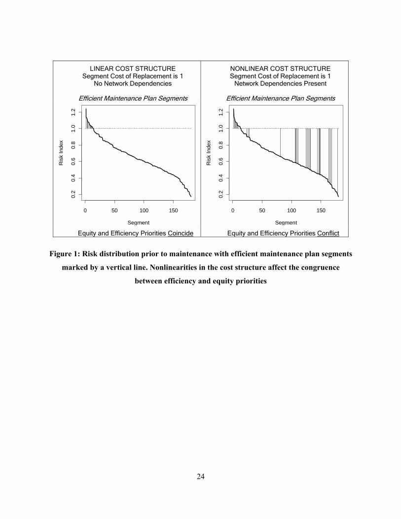
Consider a network operator interested in finding its annual optimal maintenance plan, where

segment risk distribution is according to Figure 1. In Figure 1 segment risk is represented by a

risk index measuring the ratio of expected liability for the operator to cost of segment

maintenance. This risk index can be seen as the benefit cost ratio for the maintenance of the

individual segment. Assuming a linear cost structure where the cost of segment maintenance is

2

proportional to length and segments have equal length, the direct cost of maintenance is equal

for all segments in the network. There is a very simple and intuitive process for the selection of

the optimal maintenance plan in this case (left side of Figure 1): start with the highest risk index

segment and proceed until all segments with risk index higher than one are scheduled for

maintenance. This “greedy” algorithm achieves efficiency and equity simultaneously.

Clearly this is the most cost-efficient maintenance plan from the point of view of the network

operator. But whether this plan is equitable or not can be established only after equity is carefully

defined. If a perfect system of compensation for injuries to network neighbors exists, then the

distribution of residual risk after maintenance loses its importance. It would be unrealistic to

assume such a system exists, however, especially in the case of physical injuries and fatalities.

Thus, it is expected that residual risk distribution is expected to be an important part of optimal

network maintenance decisions. The “highest risk index first” process has the obvious attribute

that risks eliminated are higher than risks accepted during network operation. If continuing

network operation generates an essential public good, some residual risk is unavoidable. In this

common case, minimizing maximum residual risk will be viewed as an equitable decision

process from a network neighbor knowing the risk distribution, but blinded by a “Rawlsian veil

of ignorance” unaware of who is exposed to which risk. It is very easy to imagine a “veil of

ignorance” exists when high-risk locations vary from one decision period to another as well as

when network neighbors do not trust the operator.

When network dependencies are significant, the most efficient maintenance plan may look like

the one on the right side of Figure 1. Clearly, a nonlinear cost structure may result in a conflict

between equity and efficiency priorities. The most efficient maintenance plan accepts high risks

and eliminates low risks, thus violating the minimax residual risk attribute of the previous case.

Now, the operator may seek to establish that if injuries occur, compensation will be perfect or

that inequity in residual risk is justifiable by the significant shared efficiencies from exploiting

the nonlinear cost structure (reflected in lower costs of network access). Nonlinear cost structures

are associated with more complex decision processes that are not as transparent as the “highest

risk first” process. We propose a decision process that is fairly complex, but is verifiable, non-

manipulable, and permits maintenance plan overrides to impose equity constraints or

management priorities. Hence, we maintain that the proposed decision process may facilitate, not

3

hinder, acceptance of optimal maintenance plans by concerned stakeholders, external to the

organization of the network operating company.

Risk assessment, whether it is based on statistical estimation or on risk models, produces

estimates within confidence intervals or ranges of uncertainty. It is thus necessary to put risk

management decisions, hinging on imprecise risk estimates, under the test of sensitivity analysis.

The proposed decision process anticipates and facilitates sensitivity analysis. In particular, we

show that the decision model we propose is robust in the sense that it has intuitively appealing

properties in response to changes in estimated decision parameters. This is very desirable in

avoiding decision process inefficiencies resulting from protracted deliberations and high-cost

data verification, within or across the organizational boundaries of the network operator.

Up to now NTD have received little attention during budgeting. It is clear that in the execution

phase of a yearly maintenance plan one can and should avoid replicating certain expenses. But, if

NTD are not recognized during budgeting, their value may become deadweight loss. For

example, consider a plan that doesn’t identify NTD, but assigns all the work in a service

subregion to one organizational division. Employees in this division may capture the NTD value

by operating at a lower workload. If, however, the division of workload doesn’t follow the

proper boundaries, then nobody is in a position to capture the value of NTD. A telling example

of NTD value loss is having a crew dig a hole on the ground, finish some work, and then cover

the hole only to have another crew visit the same area shortly after and redig the same hole.

Investor-owned companies and many municipal companies have been operating in the past under

a rate-of-return regulation system. It is well known that the efficiency of capital investments

doesn’t receive the highest priority under cost-plus regulation. However, Crew and Kleindorfer

(2002) report that many network industries are switching from rate-of-return regulation to

incentive regulation (e.g., price caps) and therefore one can expect more attention to capital

investment efficiencies and to NTD in the years to come.

Moreover, institutional innovations in the governance of infrastructure networks (e.g.,

privatization of network assets) have intensified public interest in the physical risk resulting from

the operations of networks and the equity of its distribution. Heuristic solutions for maintenance

prioritization – often utilized in practice - are challenged not only on the basis of inefficiency,

but also on the basis of undue inequity. Crude heuristics result in inexact solutions that exhibit

4

unpredictable inconsistencies in space and time. In addition to their evident inefficiency, these

inconsistencies raise questions about maintenance prioritization being manipulable. The decision

process for maintenance prioritization we propose produces exact solutions, hence its results are

replicable. We expect that verifiability supports the legitimation of efficient network

maintenance even when the resulting residual risk distribution is unbalanced.

The importance of a legitimable and efficient decision model for network maintenance, becomes

clearer if one considers the disadvantages arising from its absence. Inefficiency, as a result of

failing to recognize the importance of NTD or due to dependence on crude heuristics, forces the

network operator to function suboptimally, with lower profitability and higher service price.

When a legitimable maintenance decision process is missing, local communities are forced to

accept an arbitrary – in their minds – allocation, even though imperfect compensation gives them

standing in the risk allocation decision. This sense of injustice results, in turn, to lack of

cooperation from local communities and thus to many long term risks for the network company,

including unnecessary friction in network expansion projects.

The multiple procedural requirements in the solution of the maintenance problem, legitimation,

allocational efficiency, non-manipulability, and decision process efficiency, are met by

following an integrative approach. It consists of three equivalent formulations, which are

presented in Section 2. First, a quadratic binary program is presented that applies if infrastructure

network topology, section maintenance costs, and expected maintenance benefits are known.

This is followed by a Rhys (1970) – Balinski (1970) model, developed for the analysis of

investments with mutually exclusive costs and dependencies in benefits. Examples of the latter

problem are the “provisioning problem” described by Lawler (2001) and Mamer and Smith’s

(1982) “repair kits.” Finally, an equivalent maximum flow – minimum cut model is developed in

order for an exact solution to be efficiently obtained. Finally, Section 2 includes a subsection

that shows how requiring the maintenance of certain segments can be handled efficiently within

the proposed solution framework.

In Section 3 submodularity and antitone difference properties are verified to hold for the problem

in hand. Using Topkis’ (1978) work, it is shown that the optimal set of arcs to be maintained

using the most conservative estimates will remain in the optimal set if benefits are revised

upwards. The latter property facilitates sensitivity analysis in response to often occurring

5

changes in benefit parameters. Furthermore, this property can be utilized to obtain the Benefit-

Cost efficiency frontier for this problem quite easily, an essential part of a budgeting exercise.

Section 4 includes a complete analysis of the optimal network maintenance problem employing

our solution process to a fictitious network with 180 segments. In addition, Section 4 includes a

comparison of common general purpose mathematical programming solvers against the proposed

solution process with respect to effectiveness in reaching the optimum. Section 5 concludes.

2. Formulations of the maintenance problem

2.1. Binary Programming Formulation

Let the undirected network describe the infrastructure network under

study, where V is its node set, E is its arc set, and its parameters are given as follows:

δδ bbccEVG rr ,,,,,≡

+ℜ→Ecr : is the local maintenance cost function.

+ℜ→Ec :δ is the excess cost of replacement function. To restore arc e to an “as new”

condition the amount is required. ( ) ( )ececr δ+

+ℜ→Ebr : is the function assigning expected savings in emergency repair cost after local

preventive maintenance.

+ℜ→Eb :δ is the function assigning additional expected savings after equipment renewal in

excess to the ones resulting from local maintenance. If arc e is restored to an “as new” condition,

then the total savings in expected emergency repair costs is given as ( ) (ebebr δ+ ) . All costs and benefits are nonnegative.

The savings in emergency repair costs are usually calculated by multiplying the typically very

high cost of emergency repair (includes possible liabilities) by the expected reduction in failure

probability after maintenance. Risk assessment studies may provide estimates for failure

probabilities without maintenance, after local maintenance, and after preventive replacement

(renewal). Typically preventive replacement results in lower failure probabilities than local

maintenance; therefore it is reasonable to assume takes nonnegative values only. δb

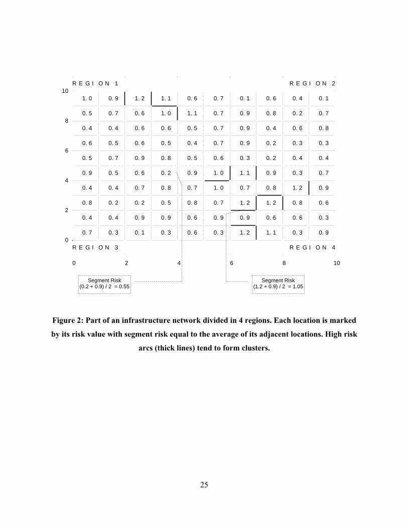
An example of an infrastructure network appears in Figure 2, where a fictitious natural gas

6

pipeline servicing a service area is depicted. High-risk segments, and thus candidates for

preventive maintenance in the short term, are drawn in thick lines. It is clear that the ratio of

high-risk segments to total number of segments should be small in a well-maintained network.

The risk of each segment is calculated as the average of the risk in its surrounding

neighborhoods. Hence, high-risk segments tend to be close to each other forming clusters, as in

Figure 2. The network is divided into four regions within which setup discounts apply. This

representation of the network may lead the reader to believe that another equity concern is also

important to consider, transboundary risk. In many types of network maintenance problems

transboundary risks are not significant. For instance in railroad safety, risk has more to do with

the number of crossings than the concentration of traffic on the one or the other side of the rail

line. In another example, natural gas distribution, risk is highly concentrated within a narrow

strip of land surrounding the pipeline, thus the stakeholders are essentially located on the

pipeline and not far away.

In some cases, however, transboundary risk is important. It is well known that divided highways

tend to also divide cities in dissimilar sections with respect to income (or ethnic origin). Risks to

property values from highway traffic may be very pronounced on the one side of the network

segment and non existent on the other side. Policies guided by average risk considerations may

lead to friction from both a rich area regarding noise reduction walls as inadequate and from its

neighboring poor area regarding, say, noise reduction walls as expensive. In these transboundary

risk cases, though, more policy options exist (e.g., raising a taller noise reduction wall only on

the one side), thus a different analysis outside the scope of our paper is required.

NTD in maintenance investments are defined by the following two functions:

Contiguity Discount Function +ℜ→Ecd 2:

( fedc , ) is the cost that will not be replicated, if the contiguous arcs e and f are both replaced:

( ) )(,:0, vfeVvfedc θ∈∈∃⇒> , where the incidence sets )(vθ are defined as

( ) ( ) ( ) ( ) ( ) EvhVhvhEhvVhhvvVv ∈∈∪∈∈≡∈∀ ,,:,,,:,θ .

Two-way contiguity discounts are meant to exist for contiguous (or possibly near contiguous)

arcs. No computational problem, however, arises in solving the maintenance problem, if the

latter restriction is relaxed. Also, ( ) 0=∈∀ edEe c .

7

If two contiguous arcs e and f are to be replaced, then their replacement cost will be:

. ( ) ( ) ( ) ( ) ( )fedfcfcecec crr ,−+++ δδ

Setup Cost Discount Function +ℜ→Π×Eds :

Where Π is a partition of physical network arcs to subregions according to the structure of setup

costs: . ⎪⎭

⎪⎬⎫

⎪⎩

⎪⎨⎧

=∅=′∩⊂′≡ΠΠ

ERRRERR U,:, ( )Red s , is the savings in replacement costs for

any arc after the cost is paid once. If are arcs to be replaced and the cost

is paid, then the resulting total cost of replacement excluding contiguity discounts for

region R will be:

Re∈ ( )Rcs RS ⊂

( )Rcs

( ) ( ) ( )( ) ( )∑ +−+∈Se

ssr RcRedecec ,δ . The setup cost discounts are positive only

in the neighborhood they refer to, i.e.: ( ) 0, =⇒∉ RedRe s .

It may be assumed that E is ordered according to some convention, so that is the i( ) Ee i ∈ th

section in the accepted order. Similarly, ( ) Π∈jR is the jth region according to some accepted

ordering. Define three cost vectors of magnitude E , E , and Π , respectively as:

( ) ( )( )iriec=rc , ( ) ( )( )ii

ecδ=δc , ( ) ( )( )jsjRc=sc . Also, , , and are rB δB cD [ ]EE × m

and sD a

atrices

[ ]E m iven as follows: Π× atrix g

( ) ( )( ) ( ) 0, =≠∀= ijirii jieb rr BB ; ( ) ( )( ) ( ) 0, =≠∀= ijiii jieb δδ BB δ

( ) ( ) ( ) ( )⎩⎨⎧ <∀

=otherwise0

, jicij

eedjicD ; ( ) ( ) ( )( )kisik Red ,=sD

Compacting cost-benefit data further with: 0ccc

c

s

δ

r≥= , and

the total maintenance costs are given by:

0000

DDB00B

B scδ

r≥

⎥⎥⎥

⎦

⎤

⎢⎢⎢

⎣

⎡=

xBxxcT TT −= (1)

Where the binary decision vector, x , has magnitude ( )Π++ EE and is comprised of 0s and

8

1s as follows:

( ) 11: =≤≤∀ iEii x if arc is to be locally maintained ( )ie

( ) 12: =⋅≤<∀ iEiEi x if arc ( Eie − ) is to be replaced

( ) 122: =Π+⋅≤<⋅∀ iEiEi x if the setup cost is paid in region ( )EiR ⋅−2

The first row of blocks in the benefit matrix B contains nonzero elements in the diagonal because

no interaction in local-maintenance benefits is considered. In contrast, B’s third row contains

only zero elements, as the benefits of setup discounts are realized though interactions only. The

second block row in B contains no 1s in the diagonal and captures the structure of benefit

interactions. Excess benefits in accrue only if both decision variables for local maintenance

and excess work for renewal are set to 1.

δB

Formulating as a lower triangular matrix assures no double counting of contiguity discounts

and economizes in calculations. Finally, applies setup cost discounts to renewal jobs only

and not to local maintenance, as appears to be the case in practice. No computational problem

arises, however, if setup discounts can be realized in local maintenance.

cD

sD

Now the maintenance cost minimization problem becomes:

(Prob. 1)

xBxxcx

TT −∈min

1,0 K with Π++= EEK

It is reasonable to assume that discounts do not exceed full cost in the following sense:

[ ] 1DDc scδ ⋅> (2)

Typically, contiguity and setup discounts are but a fraction of the total

maintenance/reconstruction cost needed to return a defective segment to ``as new’’ condition, if

not an order of magnitude less. In addition, the cost of local maintenance is also a small fraction

of reconstruction cost. Hence, in practice (2) is satisfied by a wide margin. Regularity

assumption (2) is important though, in that it guarantees that no optimal solution to Problem 1

has the form: ( ) ( ) EiiEii +<≤≤∃ ** xx,1: which would have no meaning in practice.

The cost vector is likely to be easy to estimate. It is rather difficult, however, to estimate the

Benefit Matrix, mainly because of uncertainties in the assessment of failure probabilities and

9

consequently in the calculation of expected emergency repair costs. Handling uncertainty in

benefits is discussed in Section 3.

2.2. Rhys-Balinski Formulation

Equation (1) will be put in the form used by Balinski (1970) in his selection problem. Balinski

(1970) generalized Rhys’ (1970) optimization problem for investments with mutually exclusive

costs but possibly not itemizable benefits. Without loss of generality we may use

as the set of possible maintenance investment opportunities in Problem 1. The cost of each

investment is

KH ,...,2,1=

Hk ∈ ( ) ( ) 0≥=′ kkc c . The benefit form each investment set H⊂σ is

( ) ( ) ( ) 0≥=′ σσσ xBx Tb , where ( )σx is the indicator vector of set σ, i.e.:

( )( ) σσσ ∈⇔=∈∀ kk k 1x .

Note that function is not difficult to construct. Only two-way benefit

interactions are relevant to the NTD problem. Thus, the cardinality of the benefit function

domain is not large:

+ℜ→⊂Λ′ Hb 2:

⎟⎟⎠

⎞⎜⎜⎝

⎛≤Λ

2H

. It is now clear that, with little computational effort, Problem 1

may be written as an optimization problem of itemizable costs and possibly non-itemizable

benefits as:

(Prob. 2) ( ) ( )⎪⎭

⎪⎬⎫

⎪⎩

⎪⎨⎧

∈′−′

∈= ∑

σσ

σσ

kkcb

Hmaxarg*

2.3. Max flow – min cut formulation

Balinski (1970) has shown (see also Nemhauser and Wolsey, 1988, 694-702, for a more

instructive proof) that Problem 2 is equivalent to a maximum flow problem in an auxiliary

directed network, heretofore called Cost Benefit Network (CBN). Let bcAN ′′≡Ω ,,, be the

CBN of Problem (1-2). It can be constructed as follows:

( ) ( ) qkcHkNbNoN CB ,0:,0:, >∈≡>′Λ∈≡≡ σσ , where o is a source node and q a

sink node.

10

( ) ( ) ( ) CCCBIBB NkqkANkNkANoAA ∈≡⊂∈∈≡∈≡≡ :,,,:,,:, σσσσσ

With upper capacity limits as follows1:

( )( ) ( )

( ) ( )( ) ( ) C

I

B

AqkeifkcAkeifbAoeifb

eC∈=′∈=+′∈=′

=,,,σεσσσ

where is a small quantity. +∈Rε

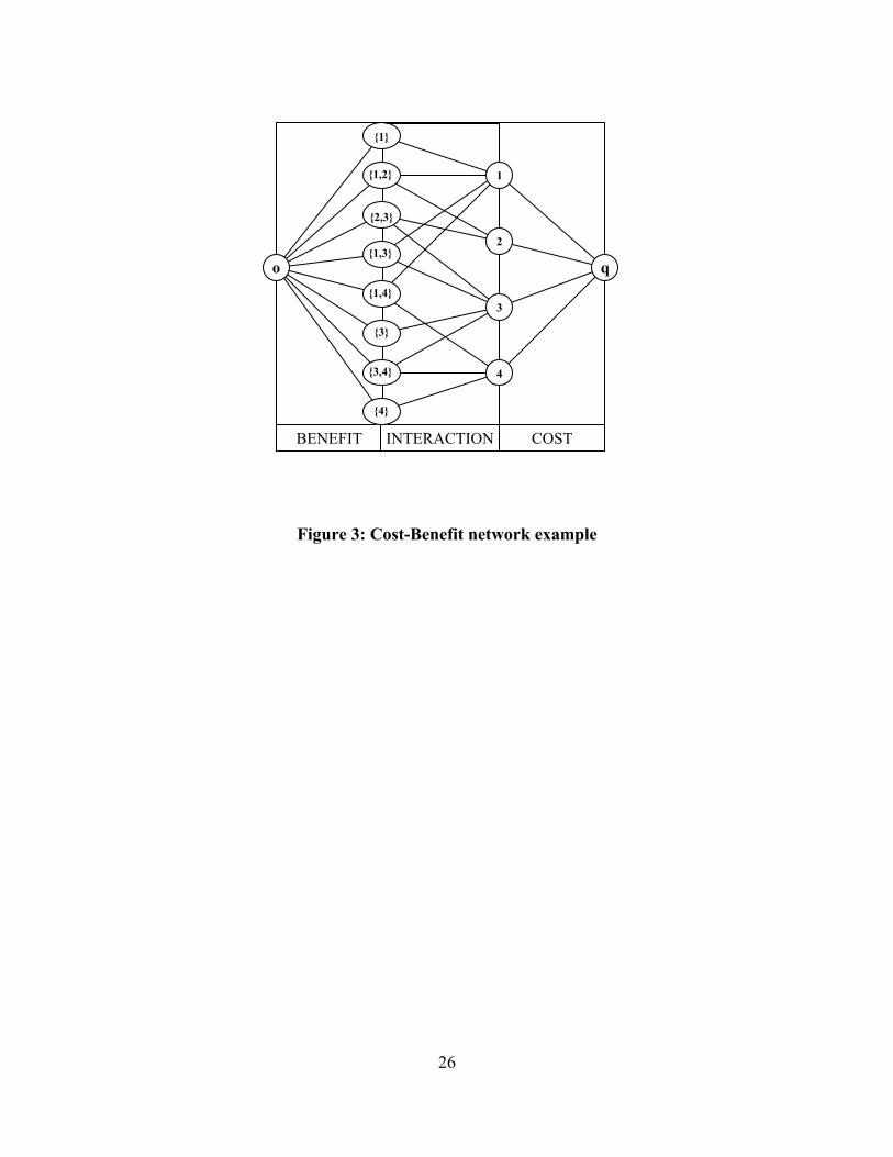
An example of a CBN is depicted in Figure 3. Let a cut separating two distinct node sets in N be

given as: ( ) ( ) YjXiAjiYXYXNYX ∈∈∈≡Γ∅=∩⊂∀ ,:,,;, . Balinski (1970) has

shown that the max-flow/min-cut problem below reveals the solution to Problem (1-2):

(Prob. 3)

( )( )⎪⎭

⎪⎬⎫

⎪⎩

⎪⎨⎧

−Γ∈∉∈⊂= ∑

XNXeeC

XqXoNXX

,,:minarg*

In particular, the cost arcs in the minimum cut reveal the optimal solution to Problem 2, which is

optimized by ( ) CNXN ∩−= **σ . Flow in the CBN corresponds to benefit and there is a one-

to-one correspondence from network segment selection to flow in the arcs. If the flow

though an arc in equals its capacity, it is called cost-limited and the net benefit of

maintaining the corresponding segment is positive. Otherwise the flow is considered benefit-

limited, thus corresponding segments are left out of the optimal maintenance list. Some arcs in

may appear to be cost-limited due to interactions with benefit-limited arcs. This problem is

avoided if is calculated by employing a depth first search for arcs with positive interaction to

cost-limited arcs.

CA

CA

CA

*σ

It is well known that solving Problem 2 as a mixed integer program with a general purpose

mathematical programming procedure, like branch and bound, will require exponentially

increasing computation time. By contrast, referring for instance to Tarjans’s (1986) analysis,

general purpose network flow algorithms would require ( )⎟⎠⎞⎜

⎝⎛ ⋅ MAO log2 time for maximum

capacity flow augmenting paths, with M being the maximum capacity limit for arcs in . CB AA ∪

1 Typically, arcs in have infinite capacity, but setting C(e) = b’(σ)+ ε for e = (σ, k) ∈ AΙΑ I obviously does not

change the nature of the problem as no arc in AI would ever be part of the minimum cut, while it eliminates

questions about the choice of a capacity that is high enough to be considered infinite.

11

Alternatively, ⎟⎠⎞⎜

⎝⎛ ⋅ NAO 2 time will be required for minimum cardinality flow augmenting

paths.

Of the two approaches we recommend the second as it does not depend on the capacities taking

integer values. Typically, rational capacities can be converted to integer after multiplication by a

constant, this however increases M and is thus counter productive. In the example we solve, the

well known algorithm by Dinic (1970) is utilized. In the past 30 years there has been

considerable progress in maximum flow algorithms. Goldberg (1998) in a recent overview of this

progress cites algorithms that are faster by about one polynomial factor, closer to ⎟⎠⎞⎜

⎝⎛ 2NO .

These methods are clearly more scalable as they permit the timely solution of much bigger

problems. In our implementation, we used a free version of Dinic’s Algorithm, available from

the Center for Discrete Mathematics and Theoretical Computer Science at Rutgers University

(dimacs.rutgers.edu), which dominated other approaches taking into account convenience and

code reliability.

It is important to note that in a well maintained network the majority of segments will not be

even considered for maintenance. An obvious simplification of the problem we consider arises

from the a priori elimination of segments in excellent condition. For these segments the risk of

failure is so small, that even if all possible network dependencies associated with them are

counted the net benefit of their replacement is still negative. Depending on the state of the

network and not only on its size the set of remaining segments (ambiguous with respect to

inclusion to the optimal maintenance list) can then become the input to the proposed selection

procedure. Hence, even though the total number of segments in a utility network may be in the

order of hundreds of thousands, one expects that the segments for which inlcusion to the optimal

maintenance list is unclear would be an order of magnitude less. In the discussion of our

illustrative example we show that results for sizable networks can be obtained with an off-the-

self computer in minutes. We expect that various factors affect computational time, including the

state of the network, the size of network dependencies, and the proximity of poor-condition

segments. Investigating in depth the determinants of computional requirements, when our

procedure is applied to a real utility network, is left outside the scope of this paper.

CBN optimization leads to exact solutions. Enumeration techniques, like branch and bound, and

12

more often crude heuristics terminate with approximations of the optimal solution. It is

important to note, that the values of total maintenance costs for near-optimal solutions may lie

close to the exact optimum, but the near-optimal arc list may be quite distinct from the optimal

list in a geographic sense. Obtaining the true optimal solution is an important advantage of the

proposed procedure, when it is applied to geographic-distribution-sensitive risk management

problems. Furthermore, exact solutions reduce significantly the latitude for manipulation in

maintenance prioritization, as other parties using the same parameters may reproduce the unique

results of the optimization procedure.

2.4. Enforced Maintenance Formulation

Finally, we show that requiring maintenance of certain segments, possibly due to equity

considerations, is very easy to do within the solution framework. Let e be the vector of enforced

maintenance, then the solution space of Problem 1 is transformed:

(Prob. 1.a) xBxxcex

TT −≥

min

But now x can be written as:

eyeexx +=+−= where 1y0 ≤≤ (3)

And the objective function of Problem 1.a becomes:

( ) ( ) ( ) ( ) ( )eBeecyByyBeBeceyBeyeyc TTTTTTTTT −+−++=++−+ (4)

Note that the third factor in the right part of (4) is a constant, hence the objective of Problem 1.a

has the same form as the objective in Problem 1. Consequently, enforcing maintenance on some

arcs does not add difficult to deal with complications to the proposed solution process.2

2 Note that significant complications arise when there are negative externalities in the benefit

function, in addition to the positive externalities assumed here. For maintenance problems, one

would normally expect only positive externalities. In the case of simultaneous negative and

positive externalities, solving the maintenance problem would probably require an altogether

different methodology (e.g., global optimization).

13

3. Sensitivity Analysis

Brumelle and Granot (1993) have analyzed in detail the effect of parametric changes in the

solution set of a “repair-kit” problem. Problem 2 belongs to the family of “repair-kit” problems

they analyze and their results are applicable to sensitivity analysis of the problem studied here. In

the next we focus first on the effect of a uniform increase in maintenance benefits in response to

a reevaluation of expected emergency repair costs. Then we discuss the selection of total

maintenance budget by varying cost of capital. We show, also, that in both cases parametric

variation leads to nested solutions.

There exist many examples of parameters that affect all service region benefits in the same

direction: for instance: upwards revision of the probability of failure after an unknown failure

mode is discovered, increases in emergency repair labor costs, increases in possible liabilities for

section failures. The revision of other parameters may or may not produce a uniform upwards

revision of benefits. For instance, changes in economic value and population densities do not

always occur in a uniform way. Some city neighborhoods experience positive growth, but other

neighborhoods may experience zero growth or decline. Uniform revisions of benefits, however,

are very common in infrastructure maintenance problems and their effect is very conveniently

obtained by the CBN procedure. This property of our solution framework is shown in the

following.

First, submodularity is verified by showing the following:

PROPOSITION 1: If 0Qdx ≥ℜ∈∈ and ,,1,0 nn is a nonnegative [ ]KK × matrix, then

( ) xQxxddQ,;x TT −=F is submodular (i.e.: ( ) ( ) ( )dQ,;xxdQ,;xdQ,;x ′∨≥′+ FFF )

( )dQ,;xx ′∧+ F ).

Where xx ′∧ , xx ′∨ symbolize respectively greatest lower and least upper bounds, following

Topkis’ (1978) notation. Topkis (1978) provides also descriptions of submodular function

properties and examples.

Proof: Without loss of generality we put vectors xx ′, in the following form:

14

4

3

2

1

xxxx

x = ,

4

3

2

1

xxxx

x

′′′′

=′ so that

⎪⎪⎩

⎪⎪⎨

⎧

=′==′==′==′=

0xx1x0x0x1x1xx

44

33

22

11

,,

and

0001

xx =′∧ ,

0111

xx =′∨ (5)

where 0 and 1 are zero and one subvectors. Matrix Q is put accordingly in the following form:

⎥⎥⎥⎥

⎦

⎤

⎢⎢⎢⎢

⎣

⎡

=

44434241

34333231

24232221

14131211

QQQQQQQQQQQQQQQQ

Q

Now by regular algebra:

( ) ( ) ( ) ( )

0111

000000Q00Q000000

0111

dQ,;xxdQ,;xxdQ,;xdQ,;x32

23

T

+′∨+′∧=′+ FFFF (6)

Q.E.D.

Therefore, the objective function of Problem 1 is submodular. This well known result is offered

to improve our exposition. Alternatively, one could verify the conditions of Topkis’s (1978)

Lemma 3.1.

PROPOSITION 2: The net cost function of Equation (1) has the antitone differences property:

( ) ( ) ( ) ( )xBxxcyByycxBxxcyByycBB,yx TTTTTTTT ′−−′−≥−−−⇒′≤≤ (7)

Proof: It suffices to show:

( ) ( ) 0≥−′−−′⇔′−′≥− xBBxyBByyByxBxyByxBx TTTTTT (8)

Breaking down the vectors y,x and the matrix ∆BBB =−′ into their components, and noting

that ( ) ( ) 0,, ≥≤∀ ijiiji ∆Byx one obtains:

( ) ( ) ( ) ( ) ( ) ( ) 0≥⎟⎠⎞⎜

⎝⎛ −=− ∑

i,jjijiij xxyy∆Bx∆Bxy∆By TT

Q.E.D.

15

Let us now consider the impact of changes in benefit arc capacities on the optimal solution. It

may be intuitive that nonnegative changes in benefit arc capacities only of the CBN will result in

a new minimum cut that contains all cost arcs obtained using the original benefit parameters.

This important fact was established by Topkis (1978), and follows directly from his results as we

now note.

The parameter set of Problem 1 is 0B,0c ≥≥ . Consider the effect of the following parametric

change:

yByycy TT* ′−= argmin

10 K, (9)

PROPOSITION 3: ⇒≥′ BB *xy* ≥

Proof: Note that , the space the decision vectors are constrained in, is a lattice. In addition,

the parameter belongs to a partially ordered set. Thus, according to Theorem 6.1 in

Topkis (1978), after the parametric change in (9), the optimal vector for the original parameter

set is no greater than the new optimal vector, provided that the following two conditions hold.

First, the objective function is submodular, which is true by Proposition 1. And second, the

antitone differences property holds, which is true by Proposition 2.

K1,0

KK ⋅ℜ∈B

Q.E.D.

Thus, if B is the most conservative benefit estimate and B’ is an upward revision of B, then all

work prescribed by *x will be prescribed also by maintenance plan *y .

*y may be computed faster if *x is known by computing ** xy − only. This process may be

extended so that the optimal maintenance plan is computed in a stepwise fashion. That is start

with a very conservative estimate of benefits, revise them upwards in steps, and in the process

increment the optimal maintenance plan. Brumelle and Granot (1993) elaborate on this approach.

The total value, V, of risk reduction (typically the net present value of expected liability

reduction) and the associated annual budget, W, are given as:

16

( ) x00000B00B

xx δ

rT

⎥⎥⎥

⎦

⎤

⎢⎢⎢

⎣

⎡=V (10)

( ) ( )xDcxxDxxcx TTT −=−=W (11)

Of particular interest is finding a budget limit W , which is not exceeded by the total cost of

maintenance under a maintenance plan x .

( ) WW =−= xDxxcx TT (12)

Fortunately, Problem 1 need not be solved under constraint (12), but its Lagragian relaxation

defines the solution to the budgeting problem. In fact, if we formulate the Lagrangian relaxation

of (12) in Problem 1, we obtain:

(Prob. 4) ( )( ) WxWxBxxcminargx TT* −λ+−= where +∈ Rλ

We can interpret λ as the network operator’s cost of capital. Varying λ from zero to some

upper bound gives rise to a feasible solution x*(λ) and an optimal budget W(x*(λ)) for each

value λ (the constant W in Prob. 4 has no effect on the solution value, of course). This

approach yields the efficient frontier in a natural way to increasing cost of capital and avoids

problems of budgeting inefficiency arising from out of frontier solutions and related duality gaps

associated with Problem 1. From a policy perspective, it is the preferred approach and the one

we follow. Reformulating Problem 4 by multiplying with ( )λγ += 11 , the results of

Proposition 3 become very clear in terms of the cost of capital approach embodied in Prob. 4.

(Prob. 5) ( )( ) xDBDxxcx TT*γ −+−= γminarg where ( ]1,0∈γ

PROPOSITION 4: ( ) ( )*γ

*γ

*γ

*γ xxxx ′′ ≤≤⇒′< WWandγγ

Proof: The first part follows immediately from Proposition 3. For the second we use the

optimality of *γx to show that:

( ) ( ) ( )( )( ) ( )

( ) ( ) ( ) ( )( ) 0≥−−−≥−

⇒−−≥

−+−=−−

′′′

′′′′′′′

*γ

T*γ

*γ

T*γ

*γ

*γ

*γ

T*γ

*γ

*γ

T*γ

*γ

T*γ

*γ

T*γ

*γ

xDBxxDBxxx

xDBxx

xDBDxxcxxDBxx

γ

γ

γγ

WW

W

W

(13)

17

The last part of (13) follows from the fact that 0DB >− and from the first part of Proposition

4.

Q.E.D.

Hence, solving for successively higher γ , the optimal management of the network requires

higher budgets also. It is a very convenient property of our solution process that as increasing

values of γ (decreasing for the cost of capital) are tried out the optimal maintenance list is

expanded and is not altered radically. The latter property is often referred to as the “Nestedness

Property.” Furthermore, due to cost structure submodularity, as γ values increase one

conveniently obtains the cost-benefit frontier with few calculations.

4. Illustrative Example

The example described in Figure 1 and in Figure 2 is worked on using the proposed method that

prescribes first to transform Problem 1 to a maximum flow problem and then to solve using an

established algorithm. Particular attention is paid to the tradeoffs in efficiency and equity as the

benefit-cost ratio varies.

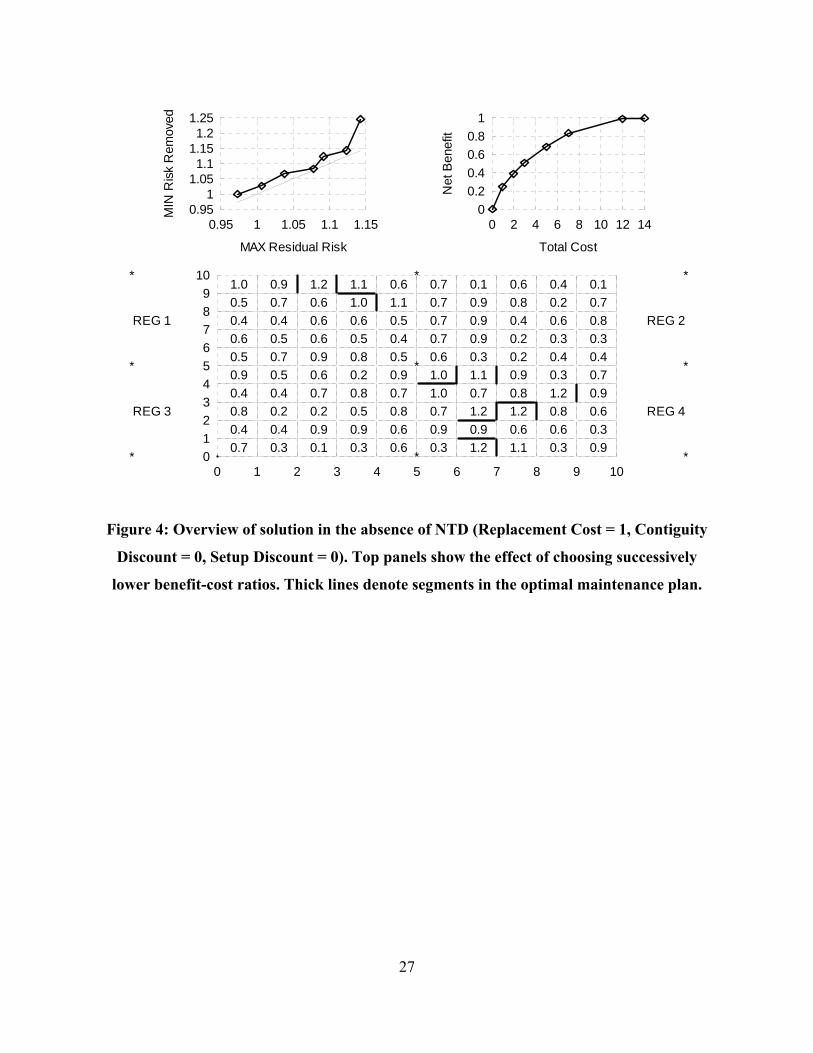
Figure 4 depicts the geographic distribution of the optimal maintenance list when NTD are not

taken into account and the cost of capital is zero (non-binding budget constraint). 14 out of 180

(7.8%) segments are in the maintenance list. From the 14 segments in the maintenance list, 11

are contiguous to another maintenance list arc (78.6%). Having so many contiguous arcs despite

the absence of NTD can be explained by the spatial dependencies in the risk structure. The

reader is reminded that the risk of each segment is the average risk of its surrounding

neighborhoods. Even though neighborhood risk was simulated as geographically independent,

segment risk by construction has an obvious dependence on geographic proximity. As high risk

segments are contiguous, segments in the optimal maintenance list are also contiguous. This

geographic dependence in segment risk is often a very realistic assumption. When NTD are

added to the maintenance cost structure the pattern of contiguous maintenance list segments will

be more pronounced.

In addition, Figure 4 depicts two panels with the equity and efficiency tradeoffs as the cost of

capital increases and in turn total budget decreases. In this “knapsack” problem, optimal

18

maintenance lists obtained by varying λ lie on the benefit cost efficiency frontier. A property

that will also apply after NTD are added. The equity tradeoff is studied using a simple metric, the

difference between the minimum risk planned for elimination (using the maintenance budget)

and the maximum risk of segments outside the maintenance list. The minimax points lie on an

increasing curve situated above the identity line (gray line in top left panel of Figure 4). Thus,

the minimum eliminated risk is higher than the maximum residual risk. This property makes it

easier for the network operator to explicate its maintenance policy.

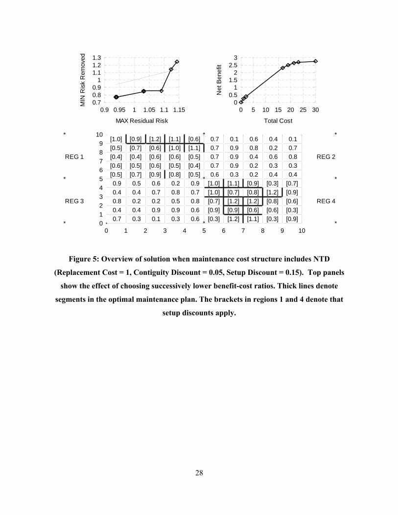
In the same format as in Figure 4, Figure 5 depicts the results one obtains after NTD are taken

into account. 34 out of 180 segments are now scheduled for maintenance. In addition, setups are

prescribed for regions 1 and 4, where neighborhood risk is put in brackets. Now all but one

segments in the maintenance list are contiguous to another maintenance list segment. With

respect to efficiency, tradeoffs are clear as all solutions generated by varying λ belong to the

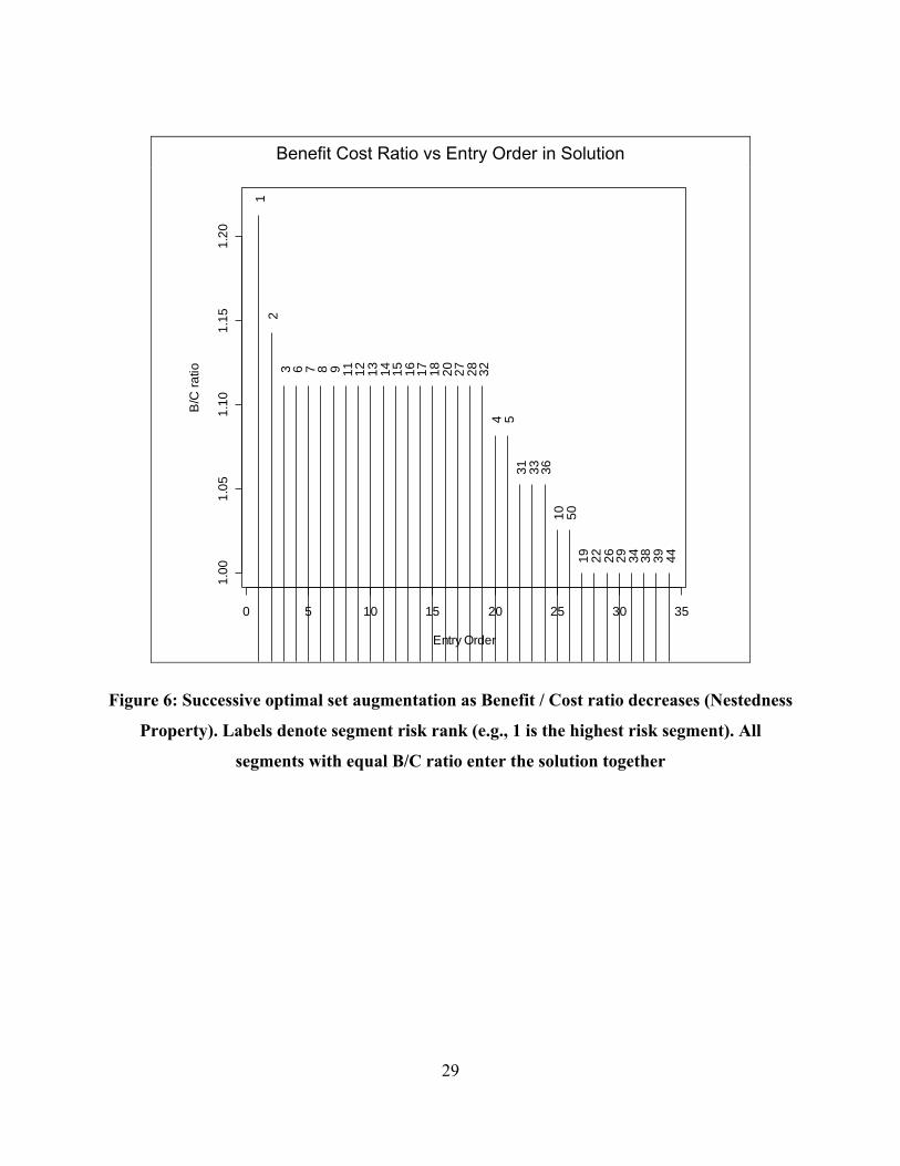
benefit-cost efficiency frontier. Figure 6 verifies the “Nestedness Property”, of the optimal

maintenance list as cost of capital increases and total budget decreases. Note, however, that risk

rank does not define entry order to the optimal solution as λ increases.

With respect to equity, note in Figure 5 that the minimax risk points form a curve that is still

increasing, but now crosses the identity line. Lower risk segments are scheduled for

maintenance, due to their being contiguous to other segments or on the regions where special

setups are prescribed. At the same time, higher risk segments that are geographically isolated are

left unmaintained. This might create friction with residents of neighborhoods exposed to the

higher residual risks. Equity tradeoffs are clear in the decision process we propose, so network

operator managers may take them into account. Consider two options to influence residual risk

distribution. First, enforce maintenance of segments with very high risk independent of whether

or not they enter the optimal (most efficient) maintenance list. And second, choose points on the

minimax curve that have low disparities between eliminated and non-eliminated risks. For

instance, choose the point (Min Removed: 0.85, Max Residual, 1.03) over the point (Min

Removed: 0.85, Max Residual, 1.09). Alternatively, network operator managers may opt for

making clear the shared benefits from the increased efficiencies due to NTD.

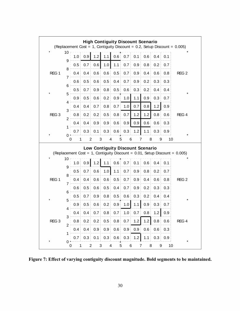
Experiments were conducted with different cost parameters for discount and contiguity. Figure 7

shows the effect of going to high (top) and low (bottom) contiguity discounts magnitude. High

19

contiguity discount leads to the optimal maintenance list forming two big clusters of segments,

in one case even joining two different regions. Regarding equity, we found in this scenario high

disparity between eliminated risk (min: 0.71) and residual risk (max: 0.93). When contiguity

discounts are lower the segments in the maintenance list are not as well connected. With respect

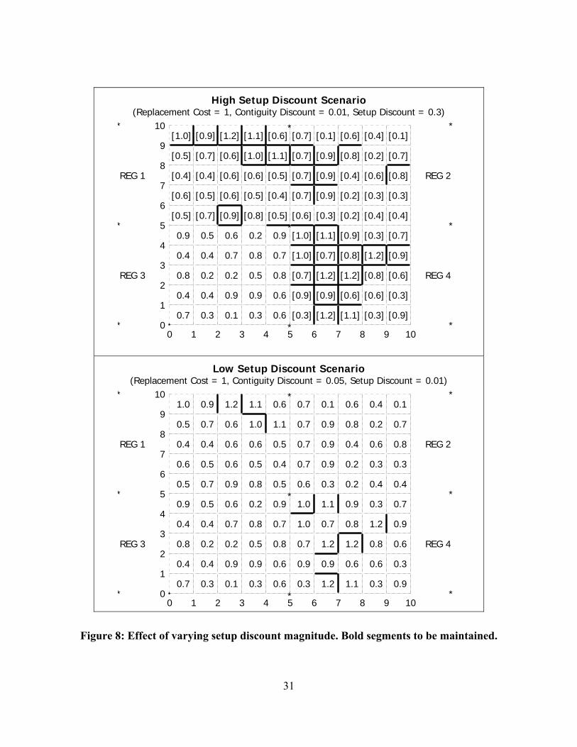
to equity, disparities exist but are not as pronounced. Figure 8 shows the effect of going to high

(top) and low (bottom) setup discount magnitudes. High setup discounts lead to an optimal

maintenance list prescribing setups in 3 out of 4 regions. With respect to equity, disparities are

also very high (Min Eliminated: 0.68, Max Not Eliminated, 0.93).

All the scenarios above were tested in a small network of 180 segments and 4 regions, which

generated a CBN of about 500 nodes and 1,200 arcs. Finding the Pareto frontier using a

conventional Linux server and unoptimized code was acheived in less than a second. The Pareto

frontier of a larger version of this network (of similar size to what may be encountered in

practical applications) with roughly 6,000 segments and about 18,000 CBN nodes was calculated

in less than 10 minutes on the same conventional machine.

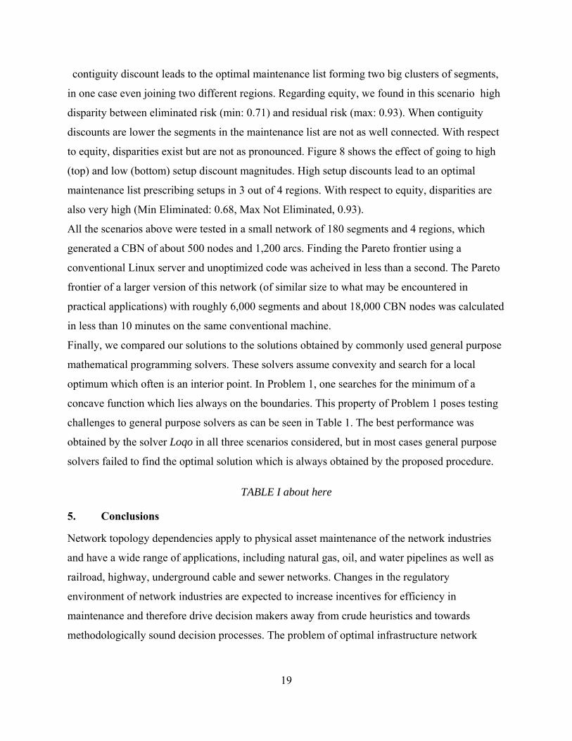
Finally, we compared our solutions to the solutions obtained by commonly used general purpose

mathematical programming solvers. These solvers assume convexity and search for a local

optimum which often is an interior point. In Problem 1, one searches for the minimum of a

concave function which lies always on the boundaries. This property of Problem 1 poses testing

challenges to general purpose solvers as can be seen in Table 1. The best performance was

obtained by the solver Loqo in all three scenarios considered, but in most cases general purpose

solvers failed to find the optimal solution which is always obtained by the proposed procedure.

TABLE I about here

5. Conclusions

Network topology dependencies apply to physical asset maintenance of the network industries

and have a wide range of applications, including natural gas, oil, and water pipelines as well as

railroad, highway, underground cable and sewer networks. Changes in the regulatory

environment of network industries are expected to increase incentives for efficiency in

maintenance and therefore drive decision makers away from crude heuristics and towards

methodologically sound decision processes. The problem of optimal infrastructure network

20

maintenance under network topology dependencies is formulated and solved by a procedure

that is computationally efficient, facilitates sensitivity analysis, and avoids manipulability.

The latter attributes of the proposed maintenance planning process are essential for success in

implementing any prioritization procedure for infrastructure maintenance. Firstly, infrastructure

networks are large in size and comprised by a vast number of elements. Therefore, computational

efficiency is a requirement. Secondly, risk estimates for the failure of network sections are rarely

robust to problem parameters and are typically given within ranges of uncertainty. Sensitivity

analysis is thus a necessary element of maintenance prioritization. Under the proposed solution,

the most frequently occurring parametric uncertainties may be analyzed very efficiently. Finally,

prioritization of physical risks that may involve loss of life, serious injuries, and significant

economic disruption is a decision likely to be challenged by many and diverse parties. The

proposed selection process produces exact solutions, which may be replicated by independent

analysts working with the same problem parameters. Near optimal solutions may be close in the

objective function range, but far apart in a geographic sense. Thus heuristic procedures, not

producing the same solution every time they are applied, may be seen as arbitrary and

manipulable. By contrast, our solution framework generates nested solutions that do not vary

radically after parametric changes. Thus, our approach provides both a logical structure and

intuitively appealing and explicable results.

Our work stresses the contribution of Operations Research and Management Science not only in

developing quantitative analysis procedures for decision support, but also in integrating decision

support systems with organizational and interorganizational decision processes. This integration

is not a trivial matter and requires in-depth knowledge of the problem context and of quantitative

analysis. An essential part of this integration is managing complexity and transparency. In our

paper we permit solution process complexity when transparency in not a requirement in order to

achieve computational efficiency. By contrast, when transparency is required, for instance when

risk equity is questioned, tradeoffs are made as clear as possible using sensitivity analysis.

Optimization procedures are designed to solve problems. They may, however, generate problems

in their implementation, raising questions of manipulability, for example, if applied

inappropriately. These side effects of quantitative decision processes are not unpredictable and

are often avoidable. Considerable effort has been allocated so that the solution procedure fits the

21

risk management problem in hand. It is often difficult to legitimate physical risk allocation to a

multitude of affected stakeholders. For network maintenance problems involving risk to the

public, it is important that procedures used be able to accommodate and transparently display the

results of budget restrictions, equity considerations and appropriate cost factors. The procedure

described here appears to satisfy these requirements.

6. References

Balinski ML (1970) On a selection problem. Management Science 17:3, 230-231.

Brumelle S, Granot D (1993) The Repair Kit Problem Revisited. Operations Research 41:5, 994-

1006.

Crew M, Kleindorfer P (2002) Regulatory Economics: Twenty Years of Progress? Journal of

Regulatory Economics (forthcoming).

Dinic EA (1970) Algorithm for Solution of a Problem of Maximum Flow with Power

Estimation. Soviet Math. Dokl., 11, 1277-1280.

Goldberg AV (1998) Recent Developments in Maximum Flow Algorithms. Technical Report

#98-045, NEC Research Institute, Inc., Princeton, NJ.

Lawler E (2001) Combinatorial Optimization: Networks and Matroids. Dover (Reprint of Holt,

Rinehart & Winston, 1976 Edition), Mineola, NY.

Mamer JW, Smith SA (1982) Optimizing Field Repair Kits Based on Job Completion Rate.

Management Science 28:11, 1328-1333.

Nemhauser GL, Wolsey LA (1988) Integer and Combinatorial Optimization, Wiley Interscience,

New York.

Rhys JK (1970) A Selection Problem of Shared Fixed Costs and Network Flows. Management

Science 17:3, 200-207.

Tarjan RE (1986) Algorithms for Maximum Network Flow. Mathematical Programming Study

26, 1-11.

Topkis DM (1978) Minimizing a Submodular Function on a Lattice. Operations Research 6:2,

305-321.

22

List of Illustrations

TABLE I: Comparison of solutions obtained by the proposed method to solutions obtained using common

general purpose solvers. Maximum net benefit is rarely approached by general purpose solvers..............22

Figure 1: Risk distribution prior to maintenance with efficient maintenance plan segments marked by a

vertical line. Nonlinearities in the cost structure affect the congruence between efficiency and equity

priorities............................................................................................................................................................24 Figure 2: Part of an infrastructure network divided in 4 regions. Each location is marked by its risk index

with segment risk equal to the average of its adjacent locations. High risk arcs (thick lines) tend to form

clusters. .............................................................................................................................................................25 Figure 3: Cost-Benefit network example .................................................................................................................26 Figure 4: Overview of solution in the absence of NTD. Top panels show the effect of choosing successively

lower benefit-cost ratios. Thick lines denote segments in the optimal maintenance plan..........................27 Figure 5: Overview of solution when maintenance cost structure includes NTD. Top panels show the effect of

choosing successively lower benefit-cost ratios. Thick lines denote segments in the optimal maintenance

plan. The brackets in the NW and SE regions denote that setup discounts apply. ....................................28 Figure 6: Successive optimal set augmentation as benefit-cost ratio decreases (Nestedness Property). Labels

denote segment indices (e.g., 146) or region codes (e.g., R4) ........................................................................29 Figure 7: Effect of varying contiguity discount magnitude....................................................................................30 Figure 8: Effect of varying setup discount magnitude............................................................................................31

23

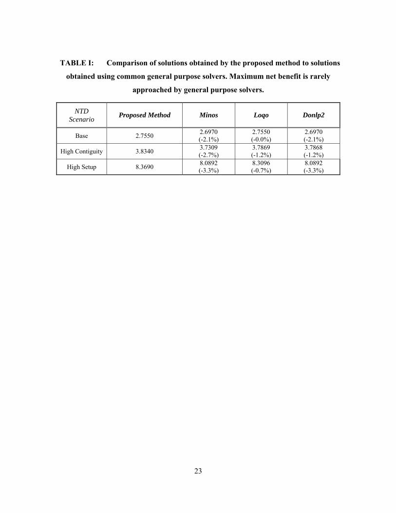
TABLE I: Comparison of solutions obtained by the proposed method to solutions

obtained using common general purpose solvers. Maximum net benefit is rarely

approached by general purpose solvers.

NTD Scenario Proposed Method Minos Loqo Donlp2

Base 2.7550 2.6970 (-2.1%)

2.7550 (-0.0%)

2.6970 (-2.1%)

High Contiguity 3.8340 3.7309 (-2.7%)

3.7869 (-1.2%)

3.7868 (-1.2%)

High Setup 8.3690 8.0892 (-3.3%)

8.3096 (-0.7%)

8.0892 (-3.3%)

24

i i

LINEAR COST STRUCTURE Segment Cost of Replacement is 1

No Network Dependencies

Efficient Ma ntenance Plan Segments

NONLINEAR COST STRUCTURE Segment Cost of Replacement is 1

Network Dependencies Present

Efficient Ma ntenance Plan Segments

0 50 100 150

0.2

0.4

0.6

0.8

1.0

1.2

Segment

Ris

k In

dex

0 50 100 150

0.2

0.4

0.6

0.8

1.0

1.2

Segment

Ris

k In

dex

Equity and Efficiency Priorities Coincide Equity and Efficiency Priorities Conflict

Figure 1: Risk distribution prior to maintenance with efficient maintenance plan segments

marked by a vertical line. Nonlinearities in the cost structure affect the congruence

between efficiency and equity priorities

25

0

2

4

6

8

10

0 2 4 6 8 10

0.7 0.3 0.1 0.3 0.6 0.3 1.2 1.1 0.3 0.9

0.4 0.4 0.9 0.9 0.6 0.9 0.9 0.6 0.6 0.3

0.8 0.2 0.2 0.5 0.8 0.7 1.2 1.2 0.8 0.6

0.4 0.4 0.7 0.8 0.7 1.0 0.7 0.8 1.2 0.9

0.9 0.5 0.6 0.2 0.9 1.0 1.1 0.9 0.3 0.7

0.5 0.7 0.9 0.8 0.5 0.6 0.3 0.2 0.4 0.4

0.6 0.5 0.6 0.5 0.4 0.7 0.9 0.2 0.3 0.3

0.4 0.4 0.6 0.6 0.5 0.7 0.9 0.4 0.6 0.8

0.5 0.7 0.6 1.0 1.1 0.7 0.9 0.8 0.2 0.7

1.0 0.9 1.2 1.1 0.6 0.7 0.1 0.6 0.4 0.1

R E G I O N 1 R E G I O N 2

R E G I O N 3 R E G I O N 4

Segment Risk (0.2 + 0.9) / 2 = 0.55

Segment Risk (1.2 + 0.9) / 2 = 1.05

Figure 2: Part of an infrastructure network divided in 4 regions. Each location is marked

by its risk value with segment risk equal to the average of its adjacent locations. High risk

arcs (thick lines) tend to form clusters.

26

BENEFIT INTERACTION COST

2,3

1,3

1,4

3

3,4

4

1,2

1

1

2

3

4

o q

Figure 3: Cost-Benefit network example

27

0123456789

10

0 1 2 3 4 5 6 7 8 9 10

0.7 0.3 0.1 0.3 0.6 0.3 1.2 1.1 0.3 0.9 0.4 0.4 0.9 0.9 0.6 0.9 0.9 0.6 0.6 0.3 0.8 0.2 0.2 0.5 0.8 0.7 1.2 1.2 0.8 0.6 0.4 0.4 0.7 0.8 0.7 1.0 0.7 0.8 1.2 0.9 0.9 0.5 0.6 0.2 0.9 1.0 1.1 0.9 0.3 0.7 0.5 0.7 0.9 0.8 0.5 0.6 0.3 0.2 0.4 0.4 0.6 0.5 0.6 0.5 0.4 0.7 0.9 0.2 0.3 0.3 0.4 0.4 0.6 0.6 0.5 0.7 0.9 0.4 0.6 0.8 0.5 0.7 0.6 1.0 1.1 0.7 0.9 0.8 0.2 0.7 1.0 0.9 1.2 1.1 0.6 0.7 0.1 0.6 0.4 0.1

*

REG 1

*

REG 3

*

*

*

*

*

REG 2

*

REG 4

*

0.951

1.051.1

1.151.2

1.25

0.95 1 1.05 1.1 1.15

MIN

Ris

k R

emov

ed

MAX Residual Risk

00.20.40.60.8

1

0 2 4 6 8 10 12 14

Net

Ben

efit

Total Cost

Figure 4: Overview of solution in the absence of NTD (Replacement Cost = 1, Contiguity

Discount = 0, Setup Discount = 0). Top panels show the effect of choosing successively

lower benefit-cost ratios. Thick lines denote segments in the optimal maintenance plan.

28

0123456789

10

0 1 2 3 4 5 6 7 8 9 10

0.7 0.3 0.1 0.3 0.6 [0.3] [1.2] [1.1] [0.3] [0.9] 0.4 0.4 0.9 0.9 0.6 [0.9] [0.9] [0.6] [0.6] [0.3] 0.8 0.2 0.2 0.5 0.8 [0.7] [1.2] [1.2] [0.8] [0.6] 0.4 0.4 0.7 0.8 0.7 [1.0] [0.7] [0.8] [1.2] [0.9] 0.9 0.5 0.6 0.2 0.9 [1.0] [1.1] [0.9] [0.3] [0.7][0.5] [0.7] [0.9] [0.8] [0.5] 0.6 0.3 0.2 0.4 0.4[0.6] [0.5] [0.6] [0.5] [0.4] 0.7 0.9 0.2 0.3 0.3[0.4] [0.4] [0.6] [0.6] [0.5] 0.7 0.9 0.4 0.6 0.8[0.5] [0.7] [0.6] [1.0] [1.1] 0.7 0.9 0.8 0.2 0.7[1.0] [0.9] [1.2] [1.1] [0.6] 0.7 0.1 0.6 0.4 0.1

*

REG 1

*

REG 3

*

*

*

*

*

REG 2

*

REG 4

*

0.70.80.9

11.11.21.3

0.9 0.95 1 1.05 1.1 1.15

MIN

Ris

k R

emov

ed

MAX Residual Risk

00.5

11.5

22.5

3

0 5 10 15 20 25 30

Net

Ben

efit

Total Cost

Figure 5: Overview of solution when maintenance cost structure includes NTD

(Replacement Cost = 1, Contiguity Discount = 0.05, Setup Discount = 0.15). Top panels

show the effect of choosing successively lower benefit-cost ratios. Thick lines denote

segments in the optimal maintenance plan. The brackets in regions 1 and 4 denote that

setup discounts apply.

29

Benefit Cost Ratio vs Entry Order in Solution

0 5 10 15 20 25 30 35

1.00

1.05

1.10

1.15

1.20

Entry Order

B/C

ratio

12

3 6 7 8 9 11 12 13 14 15 16 17 18 20 27 28 324 5

31 33 3610 50

19 22 26 29 34 38 39 44

Figure 6: Successive optimal set augmentation as Benefit / Cost ratio decreases (Nestedness

Property). Labels denote segment risk rank (e.g., 1 is the highest risk segment). All

segments with equal B/C ratio enter the solution together

30

High Contiguity Discount Scenario (Replacement Cost = 1, Contiguity Discount = 0.2, Setup Discount = 0.005)

0

1

2

3

4

5

6

7

8

9

10

0 1 2 3 4 5 6 7 8 9 10

0.7 0.3 0.1 0.3 0.6 0.3 1.2 1.1 0.3 0.9

0.4 0.4 0.9 0.9 0.6 0.9 0.9 0.6 0.6 0.3

0.8 0.2 0.2 0.5 0.8 0.7 1.2 1.2 0.8 0.6

0.4 0.4 0.7 0.8 0.7 1.0 0.7 0.8 1.2 0.9

0.9 0.5 0.6 0.2 0.9 1.0 1.1 0.9 0.3 0.7

0.5 0.7 0.9 0.8 0.5 0.6 0.3 0.2 0.4 0.4

0.6 0.5 0.6 0.5 0.4 0.7 0.9 0.2 0.3 0.3

0.4 0.4 0.6 0.6 0.5 0.7 0.9 0.4 0.6 0.8

0.5 0.7 0.6 1.0 1.1 0.7 0.9 0.8 0.2 0.7

1.0 0.9 1.2 1.1 0.6 0.7 0.1 0.6 0.4 0.1*

REG 1

*

REG 3

*

*

*

*

*

REG 2

*

REG 4

*

Low Contiguity Discount Scenario (Replacement Cost = 1, Contiguity Discount = 0.01, Setup Discount = 0.005)

0

1

2

3

4

5

6

7

8

9

10

0 1 2 3 4 5 6 7 8 9 10

0.7 0.3 0.1 0.3 0.6 0.3 1.2 1.1 0.3 0.9

0.4 0.4 0.9 0.9 0.6 0.9 0.9 0.6 0.6 0.3

0.8 0.2 0.2 0.5 0.8 0.7 1.2 1.2 0.8 0.6

0.4 0.4 0.7 0.8 0.7 1.0 0.7 0.8 1.2 0.9

0.9 0.5 0.6 0.2 0.9 1.0 1.1 0.9 0.3 0.7

0.5 0.7 0.9 0.8 0.5 0.6 0.3 0.2 0.4 0.4

0.6 0.5 0.6 0.5 0.4 0.7 0.9 0.2 0.3 0.3

0.4 0.4 0.6 0.6 0.5 0.7 0.9 0.4 0.6 0.8

0.5 0.7 0.6 1.0 1.1 0.7 0.9 0.8 0.2 0.7

1.0 0.9 1.2 1.1 0.6 0.7 0.1 0.6 0.4 0.1*

REG 1

*

REG 3

*

*

*

*

*

REG 2

*

REG 4

*

Figure 7: Effect of varying contiguity discount magnitude. Bold segments to be maintained.

31

High Setup Discount Scenario (Replacement Cost = 1, Contiguity Discount = 0.01, Setup Discount = 0.3)

0

1

2

3

4

5

6

7

8

9

10

0 1 2 3 4 5 6 7 8 9 10

0.7 0.3 0.1 0.3 0.6 [0.3] [1.2] [1.1] [0.3] [0.9]

0.4 0.4 0.9 0.9 0.6 [0.9] [0.9] [0.6] [0.6] [0.3]

0.8 0.2 0.2 0.5 0.8 [0.7] [1.2] [1.2] [0.8] [0.6]

0.4 0.4 0.7 0.8 0.7 [1.0] [0.7] [0.8] [1.2] [0.9]

0.9 0.5 0.6 0.2 0.9 [1.0] [1.1] [0.9] [0.3] [0.7]

[0.5] [0.7] [0.9] [0.8] [0.5] [0.6] [0.3] [0.2] [0.4] [0.4]

[0.6] [0.5] [0.6] [0.5] [0.4] [0.7] [0.9] [0.2] [0.3] [0.3]

[0.4] [0.4] [0.6] [0.6] [0.5] [0.7] [0.9] [0.4] [0.6] [0.8]

[0.5] [0.7] [0.6] [1.0] [1.1] [0.7] [0.9] [0.8] [0.2] [0.7]

[1.0] [0.9] [1.2] [1.1] [0.6] [0.7] [0.1] [0.6] [0.4] [0.1]*

REG 1

*

REG 3

*

*

*

*

*

REG 2

*

REG 4

*

Low Setup Discount Scenario (Replacement Cost = 1, Contiguity Discount = 0.05, Setup Discount = 0.01)

0

1

2

3

4

5

6

7

8

9

10

0 1 2 3 4 5 6 7 8 9 10

0.7 0.3 0.1 0.3 0.6 0.3 1.2 1.1 0.3 0.9

0.4 0.4 0.9 0.9 0.6 0.9 0.9 0.6 0.6 0.3

0.8 0.2 0.2 0.5 0.8 0.7 1.2 1.2 0.8 0.6

0.4 0.4 0.7 0.8 0.7 1.0 0.7 0.8 1.2 0.9

0.9 0.5 0.6 0.2 0.9 1.0 1.1 0.9 0.3 0.7

0.5 0.7 0.9 0.8 0.5 0.6 0.3 0.2 0.4 0.4

0.6 0.5 0.6 0.5 0.4 0.7 0.9 0.2 0.3 0.3

0.4 0.4 0.6 0.6 0.5 0.7 0.9 0.4 0.6 0.8

0.5 0.7 0.6 1.0 1.1 0.7 0.9 0.8 0.2 0.7

1.0 0.9 1.2 1.1 0.6 0.7 0.1 0.6 0.4 0.1*

REG 1

*

REG 3

*

*

*

*

*

REG 2

*

REG 4

*

Figure 8: Effect of varying setup discount magnitude. Bold segments to be maintained.