Optimizing Roof Maintenance and Replacement Decisions

ABSTRACT

AL-IBRAHIM, ANWAR A. Optimizing Roof Maintenance and Replacement Decisions. (Under the direction of Dr. David W. Johnston.)

The objective of this research is to develop a Decision Support System that helps

allocation of available funds to optimize roof maintenance strategies. The Decision Support

System analyzes different maintenance alternatives available for each roof element and

chooses the alternative that maximizes the benefits due to savings resulting from postponing

element replacement.

The analysis uses the Life-Cycle Cost to calculate the Reduction in Uniform Annual

Cost (RUAC) that is used as the economical decision criterion to select the most economical

maintenance alternative for each roof element at different condition states. The analysis

utilizes integer linear programming to optimize the selection of maintenance actions for the

different elements by maximizing the RUAC under budgetary constraints. Excel and AMPL

software are used to implement the analysis.

This study uses the roofing systems of 28 buildings on the North Carolina State

University campus as a model to develop the Decision Support System. Parameters

necessary to develop the model are estimated. The analysis is tested on the available data

base.

OPTIMIZING ROOF MAINTENANCE AND REPLACEMENT DECISIONS

by

ANWAR AL-IBRAHIM

A dissertation submitted to the Graduate Faculty of North Carolina State University

in partial fulfillment of the requirements for the Degree of

Doctor of Philosophy

CIVIL ENGINEERING

Raleigh

2005

APPROVED BY:

Dr. David W. Johnston Dr. Salah E. Elmaghraby Chair of Advisory Committee

Dr. Michael L. Leming Dr. John W. Baugh

ii

This work is dedicated to my dearly loved parents Adel Al-ibrahim and Maria

Gallerani who supported me spiritually and financially throughout my journey.

iii

BIOGRAPHY

Anwar Adel Al-ibrahim was born in Stillwater, Oklahoma on September 21, 1975.

At the age of four she moved back to Kuwait were she was raised. She graduated from high

school and applied to Kuwait University. She was accepted to study construction

engineering and management at the Department of Civil Engineering. She graduated in June

1998. In January 1999, she left Kuwait for the United States of America to pursue her higher

education in Construction Engineering and Management with a full scholarship granted to

her from Kuwait University.

She accomplished her Master of Science degree from Oregon State University on

November 15, 2000 under the direction of Dr. Neil Eldin. In January 2001, she had started

her Doctor of Philosophy in Civil Engineering at North Carolina State University under the

direction of Dr. David W. Johnston.

Her research interest is optimizing maintenance work on buildings. She will be a

faculty member at the Kuwait University in Kuwait.

iv

ACKNOWLEDGEMENT

I would like to take this opportunity to thank all those who helped me through out this

research. In particular, I would like to express my appreciation to Dr. David W. Johnston for

his guidance and continuous support all the way. I also would like to express my

appreciation to the other members of my committee: Dr. John W. Baugh, Dr. Michael L.

Leming and Dr. Salah E. Elmaghraby.

I would like to thank my family for their continuous support. My father Adel Al-

ibrahim and my mother Maria Gallerani for their constant encouragement and continuous

support throughout my journey. My brothers Mishel Al-ibrahim for his help in writing the

Visual Basic program, Khalid and Fahed Al-ibrahim for being there for me when I needed

them.

I also would like to thank my husband Sager Al-ghanim for being a source of

encouragement in the past 3 years, believing in me and being the deriving force toward

finishing this degree.

A special acknowledgment goes to Mr. David Hatch and the people working at the

Department of Maintenance and Repair for their time and help in providing the required

information, Dr. Neil Eldin for his continues support and valuable advices, my dear friend

Dr. Safa Amer who always was there for me when I needed a friend, Zohreh Asgharzadeh

Talebi for her help and support, Al-jarrad family for embracing me as their daughter and to

all my friends and family back in Kuwait

Finally my love goes to my new born daughter, Zain Al-ghanim for being the light of

my life.

v

TABLE OF CONTENTS

Page

LIST OF TABLES ................................................................................................. ix LIST OF FIGURES ................................................................................................. x LIST OF NOTATION................................................................................................. xi 1. INTRODUCTION................................................................................................. 1 1.1 Problem Statement........................................................................................ 1 1.2 Research Objective ....................................................................................... 2 1.3 Overview of Proposed Model ....................................................................... 3 2. LITERATURE REVIEW...................................................................................... 4 2.1 Related Literature in Roof Management ....................................................... 4 2.1.1 RoofManager .................................................................................... 4 2.1.2 Garland Roof Asset Management Program (RAMP) Computer Software............................................................................................ 5 2.2 Related Literature in Roof Maintenance........................................................ 5 2.2.1 Roofer............................................................................................... 5 2.3 Related Literature in Bridge Management..................................................... 9 2.3.1 INCBEN ........................................................................................... 9 2.3.2 OPBRIDGE ...................................................................................... 11 2.3.3 Bridge Maintenance Level of Service Optimization Based on an Economical Analysis Approach......................................................... 11 2.4 Economic Analysis Decision Criteria............................................................ 12 2.4.1 First-Cost Analysis............................................................................ 13 2.4.2 Life-Cycle Cost Analysis .................................................................. 13 2.4.3 Simple Benefit-Cost Analysis............................................................ 14 2.4.4 Incremental Benefit-Cost Analysis .................................................... 14 3. ROOF COMPONENTS ........................................................................................ 15 3.1 Low-Slope Roofs.......................................................................................... 15 3.1.1 Roof Decks ....................................................................................... 15 3.1.2 Vapor Retarder.................................................................................. 16

vi

3.1.3 Roof Insulation ................................................................................. 17 3.1.4 Roof Membrane ................................................................................ 18 3.1.5 Roof Covering or Surfacing .............................................................. 18 3.2 Steep-Slope Roofs ........................................................................................ 19 3.2.1 Roof Covering .................................................................................. 22 3.2.2 Underlayment ................................................................................... 22 3.2.3 Insulation .......................................................................................... 22 3.2.4 Roof Deck......................................................................................... 22 3.3 Other Roofing Components .......................................................................... 22 3.3.1 Drainage System............................................................................... 23 3.3.2 Roof Flashing.................................................................................... 24 4. METHODOLOGY................................................................................................ 26 4.1 Identification and Selection of Maintenance Elements .................................. 26 4.1.1 Element Rate of Deterioration ........................................................... 27 4.1.2 Element Service Life......................................................................... 27 4.2 Element Condition State ............................................................................... 30 4.3 Element Maintenance Action........................................................................ 31 4.4 Annual User Cost ......................................................................................... 34 4.4.1 Cost Damage of Building Interior...................................................... 34 4.4.2 Element Condition State Damage Factor (ECSDF)............................ 35

4.5 Equivalent, Uniform Annual Cost Calculations for Maintenance Action Alternatives ................................................................................................. 36

4.5.1 Element Replacement Alternative ..................................................... 37 4.5.2 Major Maintenance Alternative ......................................................... 42 4.5.3 Do-Nothing Alternative..................................................................... 44 4.6 Reduction in Equivalent Uniform Annual Costs............................................ 46 4.7 Reduction in Re-roofing Uniform Annual Costs ........................................... 47 4.8 Projection of Future Element Condition State .............................................. 48 4.8.1 Initial Distribution............................................................................. 49 4.8.2 Transition Matrix .............................................................................. 50 4.9 Optimizing Model ........................................................................................ 54 4.9.1 Maximizing Total Reduction in EUAC ............................................. 54 4.9.2 Maximizing Total Amount of Reduction in Re-roofing Costs............ 56

vii

5. INVENTORY, CONDITION AND COST DATA ................................................ 57 5.1 Number of Building and Buildings Roof Sections......................................... 57 5.2 Number of Maintenance Elements ................................................................ 57 5.3 Quantity of Maintenance Elements at Each Condition State.......................... 60 5.4 Real Rate of Return ...................................................................................... 61 5.5 Average Condition State Service Life ........................................................... 63 5.6 Unit Cost of Maintenance Action.................................................................. 64 5.7 Equivalent Uniform Annual Cost.................................................................. 64 6. MODEL DEVELOPMENT................................................................................... 65 6.1 Optimizing Roof Maintenance Using Separated and Combined Budgets....... 65 6.2 Excel Operations .......................................................................................... 66 6.3 Ampl Operations .......................................................................................... 72 6.4 Separated Budget Optimization..................................................................... 74 6.4.1 First Year Analysis............................................................................ 77 6.4.2 Remaining Years Analysis ................................................................ 78 6.5 Combined Budget Optimization.................................................................... 79 6.5.1 First Year Analysis............................................................................ 80 6.5.2 Remaining Years Analysis ................................................................ 81 7. ANALYSIS AND RESULTS................................................................................ 84 7.1 Separated Vs. Combined Budgets ................................................................. 84

7.2 Sensitivity of User Costs and Element Weighted Average Condition State to Budget Reduction and Increase..................................................................... 87 7.2.1 User Costs Sensitivity to Budget Levels ............................................ 87 7.2.2 Element Weighted Average Condition State Sensitivity to Budget Levels ............................................................................................... 92

viii

7.3 Sensitivity of User Costs and Element Weighted Average Condition State to Real Rate of Return ...................................................................................... 98 7.3.1 User Cost Sensitivity to Real Rate of Return Changes ....................... 98 7.3.2 Element Weighted Average Condition State Sensitivity to Real Rate of Return Changes............................................................................. 100

8. CONCLUSIONS AND RECOMMENDATIONS ................................................. 103

8.1 Conclusions ................................................................................................. 103 8.2 Recommendations ........................................................................................ 104

9. REFERENCES ................................................................................................. 106 APPENDIX A ................................................................................................. 108 APPENDIX A1 MAUCST Matrices .................................................................. 109 APPENDIX A2 EUAC Matrices ........................................................................ 116 APPENDIX B ................................................................................................. 123 APPENDIX B1 ................................................................................................. 124 Appendix B1.1 Visual Basic Code (VB)...................................................... 124 Appendix B1.2 Visual Basic Code 1 (VB1)................................................. 127 Appendix B1.3 Visual Basic Code 2 (VB2)................................................. 130 Appendix B1.4 Visual Basic Code 3 (VB3)................................................. 131 Appendix B1.5 Visual Basic Code 4 (VB4)................................................. 133 APPENDIX B2 ................................................................................................. 134 Appendix B2.1 Optimization Model Created by VB and VB1 ..................... 134 Appendix B2.2 Optimization Model Created by VB3.................................. 161 APPENDIX B3 ................................................................................................. 163 Appendix B3.1 Data File for Maintenance Optimization Model .................. 163 Appendix B3.2 Data File for Re-roofing Optimization Model ..................... 164 APPENDIX C ................................................................................................. 165 APPENDIX C1 Weighted Average Condition State Sensitivity to Budget Levels 166 APPENDIX C2 Weighted Average Condition State Sensitivity to Real Rates of Return ...................................................................................... 180

ix

LIST OF TABLES Table Page 2.1 Maintenance, repair and replacement recommendations............................. 7 4.1 Element condition states and average condition state service life ............... 28 4.2 Description of condition state..................................................................... 30 4.3 Total cost of repair to building interior ...................................................... 35 4.4 ECSDF calculation ................................................................................... 38 4.5 Transition probability for maintenance element ......................................... 52 5.1 Building name and number of sections associated ..................................... 58 5.2 Maintenance element and corresponding unit measure............................... 60 5.3 Examples of element quantity distribution over different condition states .. 62 5.4 Average condition state service life for each element at each condition state ................................................................................................. 63 6.1 “Initial Quantity” data sheet ...................................................................... 68 6.2 “Initial Building Data” sheet ..................................................................... 69 6.3 Column content description for the “Initial Building Data” sheet ............... 70 6.4 “Building Data” sheet entry ...................................................................... 71 6.5 Column content description for “Building Data” sheet .............................. 72 7.1 Analysis groups ..................................................................................... 85 7.2 User costs for the separated and combined budget cases ............................ 85 7.3 User cost sensitivity to budget levels ........................................................ 88 7.4 Total cost for different budget levels ......................................................... 91 7.5 Fund expenditure for different budget levels ........................................... 92 7.6 Single-ply membrane condition sensitivity to budget level ........................ 93 7.7 Multiple-ply membrane condition sensitivity to budget level ..................... 95 7.8 Shingle condition sensitivity to budget level .............................................. 97 7.9 User cost sensitivity to Real Rate of Return .............................................. 99 7.10 Multiple-ply membrane weighted average condition state sensitivity to Real Rate of Return................................................................................ 101

x

LIST OF FIGURES

Figure Page 3.1 Formation of blister in roof membrane....................................................... 16 3.2 Vapor retarder ................................................................................ 17 3.3 Rigid board insulation ................................................................................ 17 3.4 Built-up roofing membrane........................................................................ 18 3.5 Aggregate covering ................................................................................ 19 3.6 Compact or warm roof assembly................................................................ 20

3.7 Vented or cold roof assembly .................................................................... 21 3.8 Built-in scupper and drain strainer ............................................................. 23 3.9 Counter flashing and base flashing ............................................................ 25 4.1 Element deterioration with time ................................................................ 31 4.2 Maintenance action unit cost matrix .......................................................... 33 4.3 Extension in service life due to improvement in condition state ................. 33 4.4 Element replacement cycle profile ............................................................ 37

4.5 Perpetual replacement cycle ...................................................................... 42 4.6 Major maintenance cycle profile ............................................................... 44 4.7 Do-nothing cycle profile .......................................................................... 45 6.1 Flowchart for use of Excel and Ampl to optimize roof maintenance

using separated budget approach................................................................ 75 6.2 Flowchart for use of Excel and Ampl to optimize roof maintenance using combined budget approach ............................................................... 82 7.1 User costs for the separated and combined budget cases ............................ 86 7.2 User cost difference between the separated and combined budgets ............ 87 7.3 User cost sensitivity to budget levels ......................................................... 89 7.4 Total cost for different budget levels ......................................................... 90 7.5 Fund expenditure for different budget levels ............................................. 91 7.6 Single-ply membrane condition sensitivity to budget level ........................ 93 7.7 Multiple-ply membrane condition sensitivity to budget level ..................... 95 7.8 Shingle condition sensitivity to budget level ............................................. 96 7.9 User cost sensitivity to Real Rate of Return .............................................. 99 7.10 Multiple-ply membrane weighted average condition state sensitivity to Real Rate of Return ................................................................................ 102

xi

LIST OF NOTATION

ACSSL = Average Condition State Service Life of

AMPL = A Mathematical Programming Language

ASL = Additional Service Life

AUCST = Annual User Cost

c = Element condition state before maintenance

CS = Condition State

DM&R = Department of Maintenance and Repair

DSS = Decision Support System

ECSDF = Element Condition State Damage Factor

EL = Expected Life

EUAC = Equivalent Uniform Annual Cost

EX = Extension in element service life

f = Inflation rate

FCI = Flashing Condition Index

i = Building number

ICI = Insulation Condition Index

INCBEN = Incremental Benefit-Cost

IRC = Initial Replacement Cost

j = Roof section

k = Element condition state after maintenance

l = Maintenance element

xii

LCC = Life-Cycle Cost

MA = Maintenance Action

MAUCST = Maintenance Action Unit Cost

MCST = Maintenance Cost

MCI = Membrane Condition Index

MMC = Major Maintenance Cost

OPBRIDGE = Optimum Bridge

Pcc = Probability of a condition state c quantity staying in state c after one year

Qty = Quantity

r = Nominal rate of return

RAMP = Roof Asset Management Program

RCC = Replacement-Cycle Cost

RCI = Roof Condition Index

RCIimproved = Improved Roof Condition Index

RCST = Re-roofing Cost

REUAC = Reduction in Equivalent Uniform Annual Cost

RFUAC = Re-roofing Uniform Annual Cost

RMCST = Regular Maintenance Cost

RRFUAC = Reduction in Re-roofing Uniform Annual Cost

RRR = Real Rate of Return

RSL = Remaining Service Life

s = Roof section

SL = Service Life of element

xiii

VB = Visual Basic program

X(i,j,l,c,k)= Decision variable for building i, roof section j, element l, initial condition state c,

and final condition state k

X(t) = Vector of the CS of the element at the start of year t

µc = Average years an element stays at a condition state before deteriorating to a

lower condition state

1

1. INTRODUCTION

The condition and quality of buildings mirror the quality of life and the owner’s

awareness of building maintenance [1]. Each building element has an approximate life span.

Experience has shown that proper maintenance can not only ensure a normal life span but

can add additional life to the span expected. Proper planning and allocating the right

resources for maintenance - workers, materials, equipment, and funds - will help ensure the

availability of resources when a component is to be maintained, rehabilitated or replaced [2].

During a building’s life there are many elements to be maintained. These elements

can fall under the following categories: 1) General construction (roof maintenance, window

caulking, carpet replacement, repainting, etc.), 2) Mechanical construction (HVAC, boilers,

electrical, pluming, etc.), and 3) Custodial aspects (routine cleaning services).

1.1 Problem Statement

Roof Maintenance Management is typically a major concern for the owners of

facilities. Decisions are too often made only in reaction to a problem, such as a leak. The

use of computer programs is limited to information systems that tabulate needs from

inspections and tabulate needs from maintenance schedules. When resources are limited, a

tradeoff between maintained elements will occur. The tradeoff is to give some elements

maintenance priority over other elements to stop the deterioration beyond acceptable users’

standard. Currently the tradeoff is based on expert opinion.

2

Roof Maintenance Management should be aided by a Decision Support System

(DSS) which has the capability of optimizing the work performed on each element to reduce

the elements’ maintenance life cycle costs over the long run. The tradeoff will then be based

on expected costs and benefits associated with the work performed on each element for it to

be maintained at an optimal, and no less than minimum acceptable, condition state.

1.2 Research Objectives

The objective of this research is to develop a DSS that optimizes roof element

maintenance Condition State (CS). Concepts of economic analysis will be used to evaluate

the different maintenance options. In addition, a methodology for analyzing maintenance

cost and deterioration rate data will be implemented to optimize element condition state

alternatives.

This study will be directed toward the proper allocation of funds for building roof

maintenance work for North Carolina State University buildings by using a DSS. The first

step is to identify the availability of data and information required for developing the DSS.

The DSS is then developed to optimize the allocation of available funds for proper roof

maintenance and replacement work. The system could also provide information on the

action required on a roof element depending on its status. The action suggested might be

routine maintenance or replacement, based on the level of improvement required.

3

1.3 Overview of Proposed Model

This study will use the roofing systems of 28 buildings on the North Carolina State

University campus as an inventory to develop the DSS model. The campus has many more

buildings but additional data will be needed to implement the DDS on the entire building

inventory.

The proposed model will analyze maintenance costs and deterioration rates as

obtained from the North Carolina State University Department of Maintenance and Repair

(DM&R) database or as provided by personnel working in the department. The analysis will

compare the different maintenance activities based on their costs and expected benefits to

determine the most economical maintenance action for each roof element.

The model then takes the available budget of the DM&R into consideration and tries

to optimize the choices of different maintenance actions taking into account the available

funds, and the number and quantity of roofing elements to be maintained.

4

2. LITERATURE REVIEW

2.1 Related Literature in Roof Management

Roof Management is currently performed by using computer programs that tabulate

the available resources and provide the user with a preventive maintenance program that

reduces maintenance cost. Examples of these software programs are summarized in this

section.

2.1.1 RoofManager

RoofManager [3] is a program that facilitates creation of a database of roof

information for multiple buildings at multiple sites for a single client. Information about

each roof sector is entered. Examples of the information entered are: roof area, roof age,

construction and historical data including drawings, roof designer and contractor that

installed the roof, contractors that performed any repair work on the roof, repairs performed,

unit prices, and quantities.

This software is a helpful tool used to track and manage multiple sites and buildings

and their related repair budgets, deficiencies and repair orders. In addition the database can

incorporate site plans, drawings, and digital photos. Also, this software provides the user

with reporting capabilities by providing summaries and detailed roof information to support

roofing expenditures and budgetary plans.

5

2.1.2 Garland Roof Asset Management Program (RAMP) Computer Software

This computer program creates a data base that includes construction details,

inspection reports, roof maintenance histories and digital documentation of problem areas

[4]. RAMP computer software will then analyze the data and propose recommendations

based on specific user needs, expectations, and budget. The software provides different

repair and replacement solutions. The user is then to choose which solution best fits the

available budget.

No work has been done toward maximizing the benefits gained from extending the

roof life through maintenance while working within the available budget by using an

optimization algorithmic. Parallel work is found in bridge management where research has

been done to provide systems to optimize the allocation of limited budgets to maintenance

work while maximizing the benefits resulting from the investment.

2.2 Related Literature in Roof Maintenance

2.2.1 Roofer

Roofer is a roofing maintenance management system developed by the U.S. Army

Construction Engineering Research Laboratory with the assistance of the U.S Army Cold

Regions Research and Engineering Laboratory and the U.S. Army Engineering and Housing

Support Center [5]. Its purpose is to provide engineers with data and procedures to aid in

practical decision making for cost-effective maintenance and repair of building roofs. Roofer

provides the user with a practical tool for evaluating roofs, determining maintenance

priorities, and selecting repair strategies that ensure the maximum return on investments.

6

Roofer uses a Roof Condition Index (RCI) to evaluate the overall condition of a roof

section and to compare between different roof sections. The RCI is calculated by combining

the membrane, flashing and insulation indexes, MCI, FCI and ICI respectively. Each of the

three indexes (MCI, FCI and ICI) provides a measure of the component’s ability to perform

its function, the needed level of repair and the potential for leaks. The three component

indexes have a direct relationship in determining the needs for maintenance and repair of a

roof section, where the RCI provides an overall indication of the maintenance and repair

needs. The RCI is based on a scale from 0 to 100 with 100 indicating that only routine

maintenance is needed. The three component Indexes also range numerically from 0 to 100,

where 100 represents excellent condition. The MCI and FCI [6] are determined by visual

inspection, while the ICI is determined by evaluation techniques such as infrared, electrical

capacitance or nuclear moisture measurement.

RCI is calculated using Eq. 2.1 where 70% of the total RCI weight is given to the

lowest of the three indexes (MCI, FCI and ICI), while each of the other two indexes

contribute 15% of the weighting.

RCI = (0.7 x Lowest condition index) +

(0.15 x Sum of remaining condition indexes) (2.1)

Roofer uses the RCI to describe the overall condition of a roof section and by

combining the value of the three indexes (MCI, FCI and ICI) it gives the user and indication

of the level of repair needed Table 2.1

7

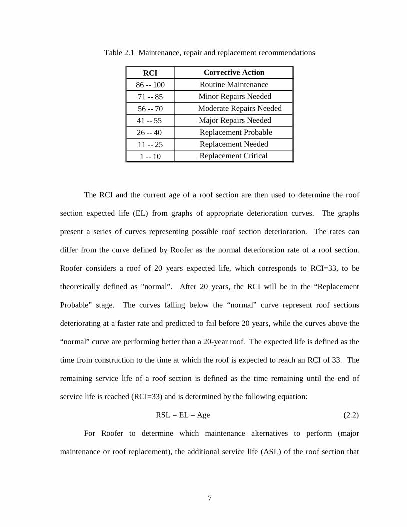
Table 2.1 Maintenance, repair and replacement recommendations

RCI86 -- 10071 -- 8556 -- 7041 -- 55 26 -- 40 11 -- 251 -- 10 Replacement Critical

Routine Maintenance Minor Repairs Needed

Moderate Repairs Needed

Corrective Action

Major Repairs Needed Replacement ProbableReplacement Needed

The RCI and the current age of a roof section are then used to determine the roof

section expected life (EL) from graphs of appropriate deterioration curves. The graphs

present a series of curves representing possible roof section deterioration. The rates can

differ from the curve defined by Roofer as the normal deterioration rate of a roof section.

Roofer considers a roof of 20 years expected life, which corresponds to RCI=33, to be

theoretically defined as "normal”. After 20 years, the RCI will be in the “Replacement

Probable” stage. The curves falling below the “normal” curve represent roof sections

deteriorating at a faster rate and predicted to fail before 20 years, while the curves above the

“normal” curve are performing better than a 20-year roof. The expected life is defined as the

time from construction to the time at which the roof is expected to reach an RCI of 33. The

remaining service life of a roof section is defined as the time remaining until the end of

service life is reached (RCI=33) and is determined by the following equation:

RSL = EL – Age (2.2)

For Roofer to determine which maintenance alternatives to perform (major

maintenance or roof replacement), the additional service life (ASL) of the roof section that

8

will result from performing a major maintenance action is calculated using the following

equation:

ASL = RSL’ – RSL (2.3)

Where RSL’ is determined from curve that requires an RCIimproved which is the

recalculated RCI for the repaired roof section

For the optimum maintenance alternative to be selected, a cost analysis should be

made to determine if the selected alternative is cost effective. The cost to repair per year of

ASL is compared to the cost per year of service life to replace the roof section by calculating

a cost ratio.

Cost of major repair/year = ASL

costrepair total (2.4)

Cost of replacement/year = years) (20 life service

costt replacemen total (2.5)

Cost Ratio = t/year replacemen ofcost

r repair/yeamajor ofcost (2.6)

It is assumed that when the cost ratio exceeds 1.0 for roofs at an early age, then

replacement is justified. However, as a roof ages, it eventually reaches a state where it will

wear out because of physical changes to the material. To compensate for this, an aging factor

is used to adjust the cost ratio as shown in Eq. 2.7. If the adjusted cost ratio is less than 0.8,

it is best to repair. If the ratio is greater than 1.2, replacement is the preferable alternative.

When the adjusted ratio falls within 0.8-1.2 the roof engineer has the option to replace or

repair.

9

Adjusted Cost Ratio = Cost Ratio + (0.01 x Age) (2.7)

Roofer is used to provide engineers with data and procedures to aid in practical

decision making for cost-effective maintenance and repair of building roofs. This system has

the following limitations:

1- The procedures used to calculate MCI, FCI and ICI are lengthy and time consuming,

2- The cost analysis is a simplified approach and does not take into account the cost of

money including inflation and discount rates,

3- The system does not allow any tracking of the deterioration of roof section elements.

4- The analysis is done on a yearly basis. There is no forecasting for maintenance work

required in the future,

5- The optional range of the adjusted cost ratio from 0.8 to 1.2 is very large. This large

range may result in a non-optimum maintenance alternative selection because it is

based only on the roof engineers’ subjective opinion.

2.3 Related Literature in Bridge Management

2.3.1 INCBEN

Farid, Johnston, Chen, Laverde and Rihani [7] investigated the applicability of the

Incremental Benefit-Cost (INCBEN) Technique in allocating limited budgets to bridge

improvement alternatives at the system level. A sample of 25 in–service bridges in North

Carolina with varying degrees of structural or functional deficiencies were investigated. The

report concluded that:

10

1. INCBEN is superior to empirical priority ranking methods used as guidelines for

knowledgeable, responsible bridge managers who select bridge improvement

alternatives under budget constraints.

2. Under budget constraints INCBEN selects near optimal sets of improvement

alternative, while it selects optimal alternative if the budget restriction is omitted.

3. The report overcame the “do-nothing’ alternative by ensuring that the least-cost

alternative is funded first. The budget balance is then allocated in such a way as

to increase the level of improvement.

The limitations of INCBEN application in a Roof Management System are similar to

those in Bridge Management Systems.

1. INCBEN does not maximize the benefits expected from improvement alternatives

selected under a limited budget.

2. INCBEN uses the total benefits (Net Benefit + Initial Cost) while the algorithm

objective is to maximize net benefits subjected to a limited budget constraint.

3. The “do-nothing” alternative should be considered when using INCBEN in a

Roof Management system for two reasons. First, it may leave out a roof that is

deficient which might cause leak and result in losses to the building users.

Second, INCBEN disregards the results of leaving the roof with no improvement

because it assumes that the benefit of such alternative is equal to zero.

4. One year is usually the horizon for a limited budget allocation produced by

INCBEN. This is considered a limited or short period. In addition to the

INCBEN possible selection of sub-optimal alternative set that has a small initial

cost but very high future cost due to the roof deterioration. This results because

11

the denominator of the incremental benefit-cost ratio only includes the first cost

for every improvement alternative.

2.3.2 OPBRIDGE

Al-Subhi, Johnston and Farid [8] developed a system which forecasts and allocates an

optimum budget for bridge maintenance and replacement (OPBRIDGE) considering both the

owner and user costs. The system determines the optimum improvement action and time for

each individual bridge in the system under various levels of service goals and funding

constraints over an analysis horizon. OPBRIDGE optimizes decisions for every year in the

analysis horizon using a 0-1 integer-linear programming formulation. At the end of every

year, OPBRIDGE ages bridges one year and predicts the required information to allow the

system to continue the analysis for the next year. The output of OPBRIDGE is a detailed

bridge by bridge recommended current and future major action. It also produces a county by

county output showing costs of major actions and the budget required for each county.

OPBRIDGE tabular and graphical outputs show the future performance level of the bridge

system over the specified study horizon.

2.3.3 Bridge Maintenance Level of Service Optimization Based on an Economical

Analysis Approach

Jabreen [9] adopted an economical analysis and decision making approach in

optimizing bridge routine and preventive maintenance levels of service. Level of service is a

trigger condition state that signals a need for maintenance effort to be applied to the bridge

12

element. In this approach, different maintenance alternatives are analyzed to select the best

levels of service that will maximize the benefits under a budget limitation.

A computer program in FORTRAN-77 was developed to implement the economical

analysis using Benefit-to-Cost Ratio and Life-Cycle Cost methods through an integer

programming algorithm to optimize the selection of levels of service for different elements.

The program determines the best economical maintenance alternative for each bridge

element at different condition states. The benefits and costs of the various levels of service

are determined through maintenance costs, replacement costs and element deterioration rates.

The parameters for estimating benefits and costs of various maintenance alternatives are

estimated.

2.4 Economic Analysis Decision Criteria

Four basic decision criteria are often used for evaluating highway improvements [7].

These criteria can also be used to evaluate roof improvement alternatives.

1. First-Cost Analysis

2. Life-Cycle Cost Analysis

3. Simple Benefit-Cost Analysis

4. Incremental Benefit-Cost Analysis

The selected criterion should provide the analyst with correct and consistent results in

attempting to:

1. Determine economic justification of proposed improvement alternatives. A

project is deemed desirable if the present value of all project benefits is equal to

or greater than the present values of all project costs

13

2. Compare merits of a group of mutually-exclusive option alternatives for selecting

the most desirable alternative.

2.4.1 First-Cost Analysis

First-cost analysis is the simplest of the four economic evaluation techniques

mentioned earlier. In this technique, alternatives are compared based on the first expenditure

on roof element improvements. The alternative with the lowest first-cost is selected as the

most economical disregarding any future costs.

In spite of being the simplest evaluation technique, first-cost analysis has the

following disadvantages:

1. Only alternatives with identical life span, performance, and maintenance needs

can be evaluated.

2. Different types of roof improvements- replacement, rehabilitation, and

maintenance- cannot be compared.

For this technique to be meaningful when comparing alternatives with different types of roof

improvements, the present value of future expenditures for each alternative must be

determined.

2.4.2 Life-Cycle Cost Analysis

Life-cycle cost (LCC) analysis combines initial and future costs of an improvement

alternative into a single present value, LCC. Future costs may include maintenance costs,

rehabilitation costs, and replacement costs minus salvage value at the end of the service life.

14

The alternative with the lowest LCC is selected as the most economical alternative. The

disadvantages of this technique are:

1. This technique cannot establish economic desirability, which is determined by

comparing benefits to costs.

2. Various alternatives must be compared over the same economic horizon (time

period), otherwise the analysis maybe biased towards the shortest time horizon.

3. This technique should only be applied to improvement alternatives which have

equal expected user benefits. Thus, life-cycle cost analysis requires that

improvement alternatives be compared under similar levels of services

2.4.3 Simple Benefit-Cost Analysis

This technique compares the benefits of improvement alternatives with their costs.

The advantages of this technique when compared to the previous two techniques are:

1. It can be applied to roofs with different levels of service because it considers user

costs as well as agency costs.

2. The analysis can be conducted at both roof and system levels.

The problem with this technique is estimating user and agency benefits in monetary terms.

2.4.4 Incremental Benefit-Cost Analysis

Incremental benefit-cost ratio is defined [7] as “the ratio of the extra benefits of

advancing from one improvement level to the next, divided by the corresponding extra cost.”

For the incremental increase in benefits to be economically justified the ratio should be

greater or equal to one.

15

3. ROOF COMPONENTS

The primary purpose of a roof system is to protect the interior of the building from

moisture and to prevent excessive heat loss. The roof structure also serves as an integral part

of the structural frame and must be designed to sustain loads due to wind, snow, and rain, as

well as to contribute to the building’s exterior appearance. Building roofs are generally

divided into two categories. Low-slope roofs with a slope of 3:12 or less, and steep-slope

roofs with a slope of more than 3:12. This chapter will cover these two types of roofs and the

roofing system components characterizing each type.

3.1 Low-Slope Roofs

A Low-slope roof is composed of several interrelated parts, and collectively these

parts are referred to as either the roof assembly or the roof system [10]. A roof assembly

includes the roof deck, vapor retarder (if present), roof insulation, roof membrane and roof

covering or surfacing. The roof system includes all the components of a roof assembly

excluding the roof deck.

3.1.1 Roof Decks

The roof deck serves as the structural foundation onto which a roof system is applied

and may provide slope. A roof deck maybe made of wood, concrete, metal, gypsum, or

lightweight cellular concrete.

16

3.1.2 Vapor Retarder

Vapor retarders are used to prevent moisture vapor within the building from

infiltrating the insulation and condensing, thereby destroying the insulating value, and

eventually causing blistering or other damage to the roof covering, Figure 3.1. The vapor

retarder may be located at various points in the roof assembly depending on the type of

construction. The most common position for vapor retarder is over the roof deck, just under

the insulation, Figure 3.2.

Pocket of trapped air andmoisture

Vapour pressure rises too quickly toescape through dense deck

Rapid expansion of trapped air andmoisture forms small blister

Partial vacuum at night drawsadditional air and water vapour intoblister from deck

Partial vacuum at night drawadditional air and water vapourthrough micro cracks

DAY

NIGHT

Figure 3.1 Formation of blister in roof membrane [11]

17

Figure 3.2 Vapor retarder [12]

3.1.3 Roof Insulation

Roof insulation provides the building with thermal resistance which will reduce the

energy used by the air-conditioning and heating systems and will result in energy cost saving.

Roof insulation is also used as a base for most membranes over any structural deck and to

create slopes on flat roofs to allow for drainage and to help control ponding during heavy

storms. Insulation is applied over the vapor barrier or directly over the roof deck. There are

four types of roof insulation:

1. Rigid board - perlite, wood fiber or polyisocyanurate foam, Figure 3.3,

2. Composite board,

3. Cellular Glass Roof Insulation, and

4. Glass Fiber Insulation boards.

Figure 3.3 Rigid board insulation [12]

18

3.1.4 Roof Membrane

Roof membranes serve as the weatherproofing component of the low-slope roof. The

membrane is installed over the insulation or directly over the roof deck. Common roof

membrane types are:

1. Built-up Roofing Membrane, Figure 3.4,

2. Thermoplastic Single-Ply Membrane,

3. Thermoset Single-Ply Roofing Membrane, and

4. Modified Bitumen Roofing Membrane.

Figure 3.4 Built-up roofing membrane [12]

3.1.5 Roof Covering or Surfacing

Roof coverings are used to protect the roof membrane from direct sunlight and to

reflect solar radiation [13]. It thus slows down weathering of the roofing membrane. Roof

surfacing also protects the membrane against casual foot traffic. Roof surfacing may include:

1. Aggregate, Figure 3.5,

2. Cap sheets, and

3. Smooth-surfaced Aggregate.

19

Figure 3.5 Aggregate covering [12]

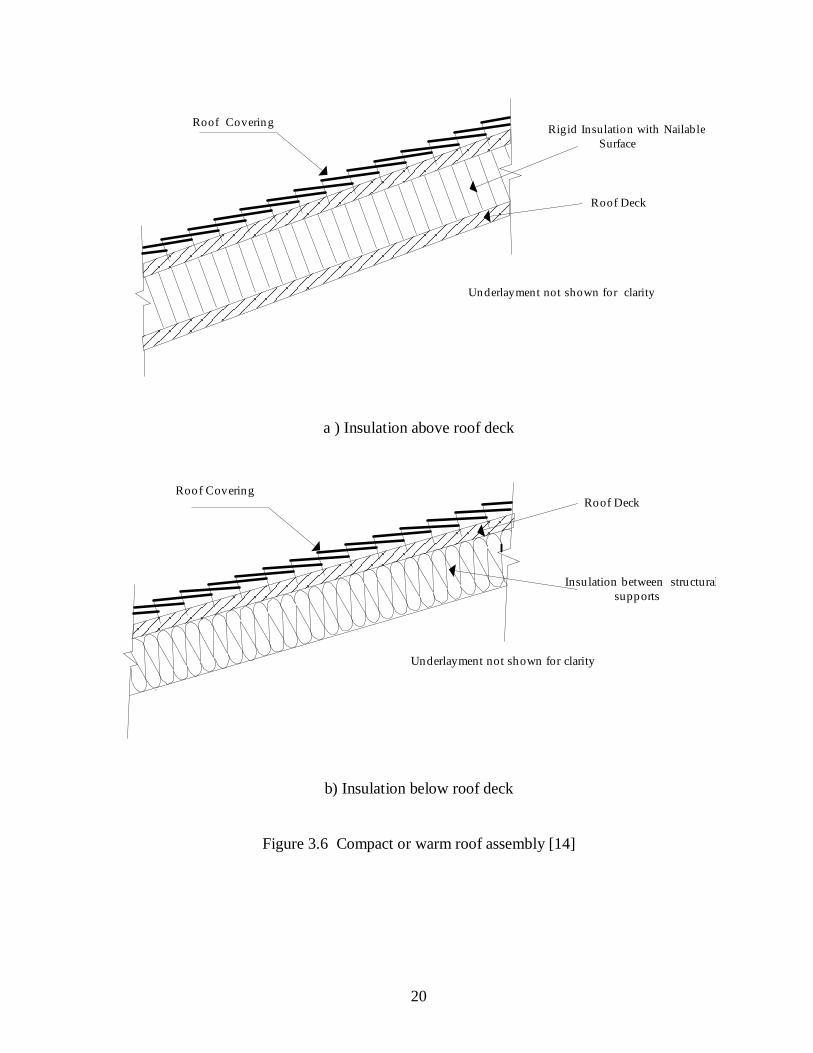
3.2 Steep-Slope Roofs

Steep-slope roofs are water shedding roof systems that function with gravity to shed

water from one course to the next, thereby draining roof surfaces. Steep-slope roofs are

composed of a roof covering, underlayment, insulation (covered by a nailable substrate if

installed on top of a roof deck) and roof deck. Steep-slope roofs are divided into two

categories. Compact, or warm, roof assemblies incorporate insulation directly above or

below roof decks as shown in Figure 3.6. Ventilated, or cold, roof assemblies have

ventilation cavities beneath roof decks. A ventilation cavity may be an attic or a vented

space just below the nailable surface of a roof covering as shown in Figure 3.7.

20

Rigid Insulation with NailableSurface

Roof Deck

Roof Covering

Underlayment not shown for clarity

a ) Insulation above roof deck

Insulation between structuralsupports

Roof DeckRoof Covering


b) Insulation below roof deck

Figure 3.6 Compact or warm roof assembly [14]

21

Ridge Vent

Roof coveringover roof deck

air flow

Vented space

Soffit vent

Insulation layer atciling level

a) Vented attic

Air Flow

Vented space

Roof deck

Insulation between structuralsupport

Roof covering over nailablesurface


b) Vented compact roof

Figure 3.7 Vented or cold roof assembly [14]

22

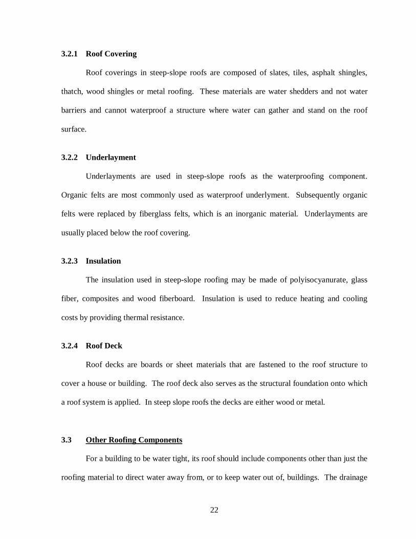
3.2.1 Roof Covering

Roof coverings in steep-slope roofs are composed of slates, tiles, asphalt shingles,

thatch, wood shingles or metal roofing. These materials are water shedders and not water

barriers and cannot waterproof a structure where water can gather and stand on the roof

surface.

3.2.2 Underlayment

Underlayments are used in steep-slope roofs as the waterproofing component.

Organic felts are most commonly used as waterproof underlyment. Subsequently organic

felts were replaced by fiberglass felts, which is an inorganic material. Underlayments are

usually placed below the roof covering.

3.2.3 Insulation

The insulation used in steep-slope roofing may be made of polyisocyanurate, glass

fiber, composites and wood fiberboard. Insulation is used to reduce heating and cooling

costs by providing thermal resistance.

3.2.4 Roof Deck

Roof decks are boards or sheet materials that are fastened to the roof structure to

cover a house or building. The roof deck also serves as the structural foundation onto which

a roof system is applied. In steep slope roofs the decks are either wood or metal.

3.3 Other Roofing Components

For a building to be water tight, its roof should include components other than just the

roofing material to direct water away from, or to keep water out of, buildings. The drainage

23

system can be considered as a first line of defense against water penetration followed by roof

flashing. The following sections will describe the drainage system and roof flashing in more

detail.

3.3.1 Drainage Systems

Drainage systems are used as the first line of defense against moisture by directing

water away from the roof and eliminating water ponding on the roof surface. Drainage

systems used in low-slope roofs differ than the drainage systems used in steep-slope roofs.

Low-slope roof drainage systems are in the interior of the roof surface with the scupper built

into the roof and the drain strainer projecting above the roof surface, Figure 3.8. The

drainage system of the steep-slope roof consists of the gutter that runs around the parameter

of the roof collecting the water moving downward due to gravity, and the downspout that is

attached to the gutter to take the water out of the gutter and down to the drainage pipe or

splash block on the ground.

Figure 3.8 Built-in scupper and drain strainer [12]

24

3.3.2 Roof Flashing

Roof flashings are used in both low-slope and steep-slope roofs wherever there is an

interruption in the roof surface. Flashing is used to seal and protect joints in a building from

water penetration. The joints created by the intersection of the roof and roof rising structures

and projections, such as parapets, hatches, skylights, chimneys, vent stacks, or towers, are

among the most vulnerable areas of roofing systems. They constantly expand and contract in

response to changes in humidity and temperature. The greater the number of such

projections, the greater the potential for serious leaks. Flashing is used at these intersections

to keep rainwater from leaking into the building. It makes joints at these junctions

watertight, while at the same time allowing the natural expansion and contraction of

materials to continue. Flashing materials are overlapped when installed in such a way as to

discourage water entrapment. Roof flashing can be divided into two groups: Vertical

Flashing and Horizontal Flashing [15].

1. Vertical Flashing: Vertical flashings are installed at upturned edges, such as walls.

Vertical Flashings are divide into three parts:

- Cant: A cant is a triangular-shaped strip made of perlite, wood fiberboard

or wood. Cants are used in corners so that flashing materials do not have

to bend so much as to cause a tear. A cant is adhered or mechanically

fastened.

- Base Flashing: A base flashing may be an extension of the roof membrane

running up to the vertical parapet wall or other projecting element or may

be of a different waterproof material that is compatible with the roofing

materials used. Base flashings are used to exclude moisture from

25

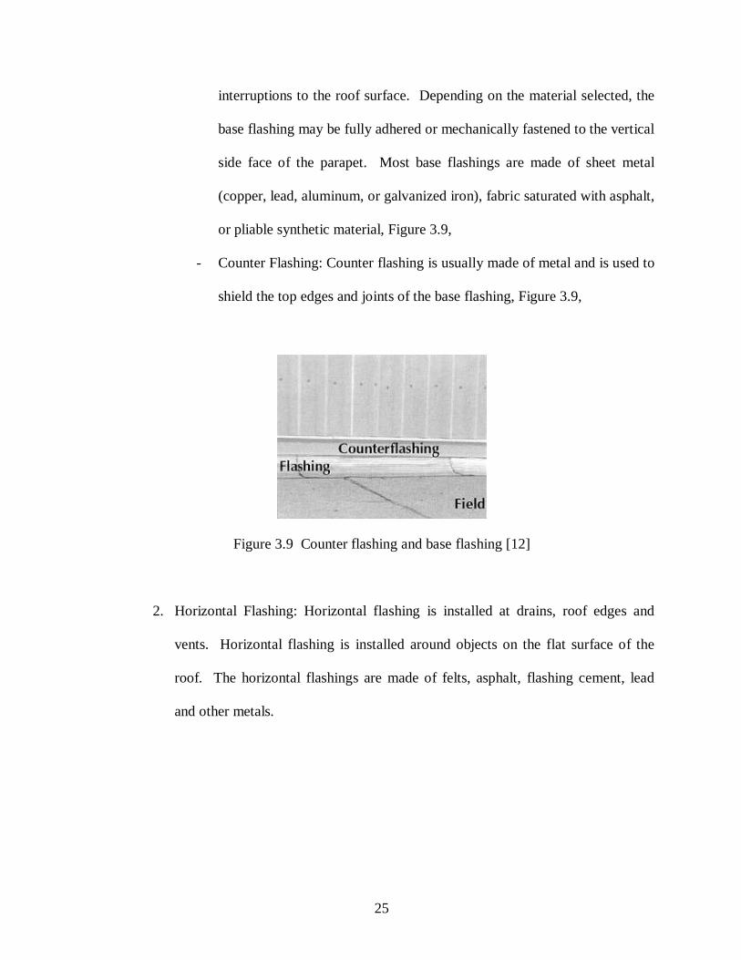
interruptions to the roof surface. Depending on the material selected, the

base flashing may be fully adhered or mechanically fastened to the vertical

side face of the parapet. Most base flashings are made of sheet metal

(copper, lead, aluminum, or galvanized iron), fabric saturated with asphalt,

or pliable synthetic material, Figure 3.9,

- Counter Flashing: Counter flashing is usually made of metal and is used to

shield the top edges and joints of the base flashing, Figure 3.9,

Figure 3.9 Counter flashing and base flashing [12]

2. Horizontal Flashing: Horizontal flashing is installed at drains, roof edges and

vents. Horizontal flashing is installed around objects on the flat surface of the

roof. The horizontal flashings are made of felts, asphalt, flashing cement, lead

and other metals.

26

4. METHODOLOGY

4.1 Identification and Selection of Maintenance Elements

The DM&R at North Carolina State University funded a roof management survey

carried out by Stafford Consulting Engineers. The survey results are stored in RoofManager

and provide a data base for multiple building roofs at different sites belonging to the

university. RoofManager also lists re-roofing costs and repair costs by item to provide the

user with additional insight into the decision of re-roof versus repair. This research will

adopt the information provided by the RoofManager database for each roof element. Missing

information is provided by the roofing expertise of the staff of the DM&R.

RoofManager also provides a list of recommended repair methods. Each group of

repair methods relates to a certain maintenance element in the roof. A maintenance element

is a physical part of a roof that requires a substantial maintenance effort [9]. The major

maintenance elements identified by the DM&R staff and provided by the RoofManager

database are used in this research. For the purpose of this research, each element is assigned

a number which is used as a reference in the optimization model developed. For each

element in the system, certain parameters are needed by the optimization which were not

available in RoofManager, particularly the element’s expected rate of deterioration and the

element’s expected service life.

27

4.1.1 Element Rate of Deterioration

Roof elements deteriorate with time. The decline in condition can be described as a

series of condition states such as those described in Table 4.1 which were developed during

this research effort. Each element will have a condition state service life at each condition

state (CS). The condition state service life is associated with the average time (in years) that

an element will stay at a condition state before declining to a lower condition state. The

average condition state service lives presented in Table 4.1 were estimated by the DM&R

roofing staff personnel. The element average condition state service life at a condition state

will be characterized by ACSSL(l,c) where (l) represents the element and (c) is the condition

state before maintenance.

4.1.2 Element Service Life

Service life is another important parameter of an element. Element service life is the

time span that a roof element can serve its purpose before it needs replacement [9]. The

element service life can be calculated from:

SL(l) =∑5

),(c

cACSSL l + EX(l,c,k) (4.1)

Where,

SL(l) = Service life of element (l) starting new,

ACSSL(l,c) = Average Condition State Service Life of element (l) at condition

state (c) during first cycle of deterioration,

28

EX(l,c,k) = Extension in element (l) service life when the condition state is

increased from condition state (c) to condition state (k) after first

cycle of deterioration.

Table 4.1 Element condition states and average condition state service life

5 New/excellent Membrane- New condition 13.00

4 Loose/dry Membrane Lap or wrinkled/ridging Membrane/ slightly deteriorated- No deficiency

5.00

3 Infiltration of water in roof system/ partially deteriorated- Deficient with no damage 2.00

2 Infiltration of water in building- Damaged 1.001 Deteriorated/damaged Membrane- Useless/ non-functional 0.005 New/excellent Membrane- New condition 18.00

4Loose/dry Membrane Lap or wrinkled/ridging Membrane/ slightly deteriorated- No deficiency 6.00

3 Infiltration of water in roof system/ partially deteriorated- Deficient with no damage 1.50

2 Infiltration of water in building- Damaged 0.751 Deteriorated/damaged Membrane- Useless/ non-functional 0.005 New/excellent Insulation- New condition 15.50

4 Shuffled/loose Insulation, loose Insulation fastener/ slightly damaged- No deficiency 4.50

3 Small Area of saturation/ partially damaged- Deficient with no damage 2.002 Large area of saturation- Damaged 0.751 Collapsed Insulation/ fully saturated- Useless/ non-functional 0.005 New/excellent Base Flashing- New condition 10.004 Small hair-line cracks- Deterioration with no deficiency 5.003 Wide spread cracks- Deficiency with no damage 2.002 Partially deteriorated /loose Base Flashing- Damaged 1.251 Dried/deteriorated Base Flashing- Useless/ non-functional 0.005 New/excellent Base Flashing- New condition 12.504 Small hair-line cracks- Deterioration with no deficiency 6.003 Wide spread cracks- Deficiency with no damage 3.002 Partially deteriorated /loose Base Flashing- Damaged 2.001 Dried/deteriorated Base Flashing- Useless/ non-functional 0.005 New/excellent Counter Flashing condition 5.504 Slightly deteriorated/damaged/rusted Counter Flashing- No deficiency 4.003 Partially deteriorated/damaged Counter Flashing- Deficiency with no damage 3.502 Loose Counter Flashing/severely damaged- Damaged 2.001 Missing Counter Flashing- Useless/ non-functional 0.005 New/excellent Gutter- New condition 5.004 Slightly deteriorated/loose Gutter- No deficiency 3.00

3 Partially disconnected & leaking Gutter/partially damaged- Deficient with no damage 2.00

2 Substantially disconnected & leaking Gutter/ severely damaged- Damaged 0.751 Missing or ineffective Gutter/ useless/ non-functional 0.00

No.

5

6

7

1

2

3

4

ACSSL

Counter Flashing

Gutter

Base Flashing Single-ply

Base Flashing Multiple-ply

Multiple-ply membrane

Insulation

Element Condition State Description

Single-ply membrane

CS

29

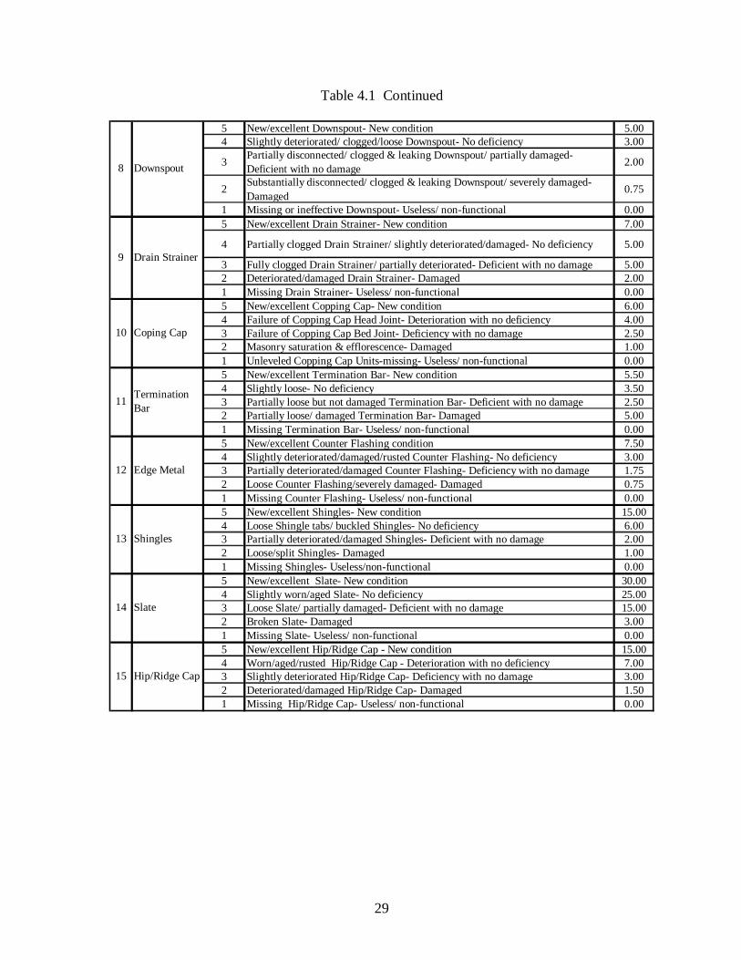
Table 4.1 Continued

5 New/excellent Downspout- New condition 5.004 Slightly deteriorated/ clogged/loose Downspout- No deficiency 3.00

3 Partially disconnected/ clogged & leaking Downspout/ partially damaged- Deficient with no damage 2.00

2 Substantially disconnected/ clogged & leaking Downspout/ severely damaged- Damaged

0.75

1 Missing or ineffective Downspout- Useless/ non-functional 0.005 New/excellent Drain Strainer- New condition 7.00

4 Partially clogged Drain Strainer/ slightly deteriorated/damaged- No deficiency 5.00

3 Fully clogged Drain Strainer/ partially deteriorated- Deficient with no damage 5.002 Deteriorated/damaged Drain Strainer- Damaged 2.001 Missing Drain Strainer- Useless/ non-functional 0.005 New/excellent Copping Cap- New condition 6.004 Failure of Copping Cap Head Joint- Deterioration with no deficiency 4.003 Failure of Copping Cap Bed Joint- Deficiency with no damage 2.502 Masonry saturation & efflorescence- Damaged 1.001 Unleveled Copping Cap Units-missing- Useless/ non-functional 0.005 New/excellent Termination Bar- New condition 5.504 Slightly loose- No deficiency 3.503 Partially loose but not damaged Termination Bar- Deficient with no damage 2.502 Partially loose/ damaged Termination Bar- Damaged 5.001 Missing Termination Bar- Useless/ non-functional 0.005 New/excellent Counter Flashing condition 7.504 Slightly deteriorated/damaged/rusted Counter Flashing- No deficiency 3.003 Partially deteriorated/damaged Counter Flashing- Deficiency with no damage 1.752 Loose Counter Flashing/severely damaged- Damaged 0.751 Missing Counter Flashing- Useless/ non-functional 0.005 New/excellent Shingles- New condition 15.004 Loose Shingle tabs/ buckled Shingles- No deficiency 6.003 Partially deteriorated/damaged Shingles- Deficient with no damage 2.002 Loose/split Shingles- Damaged 1.001 Missing Shingles- Useless/non-functional 0.005 New/excellent Slate- New condition 30.004 Slightly worn/aged Slate- No deficiency 25.003 Loose Slate/ partially damaged- Deficient with no damage 15.002 Broken Slate- Damaged 3.001 Missing Slate- Useless/ non-functional 0.005 New/excellent Hip/Ridge Cap - New condition 15.004 Worn/aged/rusted Hip/Ridge Cap - Deterioration with no deficiency 7.003 Slightly deteriorated Hip/Ridge Cap- Deficiency with no damage 3.002 Deteriorated/damaged Hip/Ridge Cap- Damaged 1.501 Missing Hip/Ridge Cap- Useless/ non-functional 0.00

13

14

15

9

10

11

12

8

Slate

Hip/Ridge Cap

Edge Metal

Shingles

Coping Cap

Termination Bar

Downspout

Drain Strainer

30

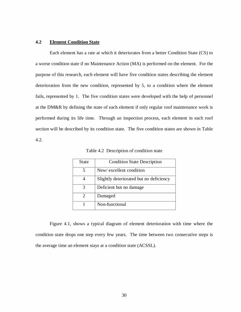
4.2 Element Condition State

Each element has a rate at which it deteriorates from a better Condition State (CS) to

a worse condition state if no Maintenance Action (MA) is performed on the element. For the

purpose of this research, each element will have five condition states describing the element

deterioration from the new condition, represented by 5, to a condition where the element

fails, represented by 1. The five condition states were developed with the help of personnel

at the DM&R by defining the state of each element if only regular roof maintenance work is

performed during its life time. Through an inspection process, each element in each roof

section will be described by its condition state. The five condition states are shown in Table

4.2.

Table 4.2 Description of condition state

State Condition State Description

5 New/ excellent condition

4 Slightly deteriorated but no deficiency

3 Deficient but no damage

2 Damaged

1 Non-functional

Figure 4.1, shows a typical diagram of element deterioration with time where the

condition state drops one step every few years. The time between two consecutive steps is

the average time an element stays at a condition state (ACSSL).

31

Time (years)

Con

ditio

n St

ate

5

4

3

2

1

Figure 4.1 Element deterioration with time

4.3 Element Maintenance Action

Each element will have one or more maintenance action (MA) alternatives at each

condition state. The higher the element condition state the lower the number of maintenance

action alternatives that will be available for the element. Each maintenance action will

require the following information:

1. The unit cost of performing the maintenance action.

Maintenance costs were usually provided from one of two sources: North

Carolina State University historical cost data or the Means Building Construction

Cost Data. RoofManager has work function codes for the types of maintenance and

repair performed on roofs. There are 162 function codes, each describing a certain

type of maintenance work item. Each group of maintenance work items generally

relates to a particular roof element. Unit costs for maintenance work function codes

will be denoted in this research by MAUCST(l,c,k) where (l) is the element, (c) is the

32

condition state before maintenance and k is the condition state after maintenance.

Figure 4.2 shows the maintenance action unit cost matrix representing the unit cost of

improving an element from a condition state (c) to a condition state (k). These unit

costs were partially available from Roofmanager and partially developed in this

research.

2. The effect of maintenance action on the condition of element.

It is assumed that each maintenance action will improve the state of the

element, which will lengthen its service life and postpone the need for replacement.

This improvement can be determined as the increase in the element condition state

after maintenance. The higher the increase in the element condition state, the higher

the cost of maintenance. For routine maintenance performed annually on each roof

section, the element condition state will not increase, but will help in slowing the

element deterioration.

Figure 4.3 shows the effect of increasing the element condition state to a higher state that

results in the extension of the element service life.

33

Condition state after maintenance (k)5

5 MAUCST(l,5,5)

4

4 MAUCST(l,4,5) MAUCST(l,4,4)

3

3 MAUCST(l,3,5) MAUCST(l,3,4) MAUCST(l,3,3)

2

2 MAUCST(l,2,5) MAUCST(l,2,4) MAUCST(l,2,3) MAUCST(l,2,2)

1

1 MAUCST(l,1,5) MAUCST(l,1,4) MAUCST(l,1,3) MAUCST(l,1,2) MAUCST(l,1,1)

$/Unit measure

Con

ditio

n st

ate

befo

re m

aint

enan

ce (c

)

Figure 4.2 Maintenance action unit cost matrix

Figure 4.3 Extension in service life due to improvement in condition state

34

4.4 Annual User Cost

Annual user cost is the cost incurred by a building user if damage occurs due to water

infiltration into the building interior. It can also be defined as the penalty paid by the agency

as result of selecting one maintenance alternative instead of the other.

Damage to a building interior is calculated by multiplying the cost of repairing a unit

area of the building interior by an Element Condition State Damage Factor. The annual user

cost is calculated as follows:

AUCST(l,c) = Damage Cost * ECSDF(l,c) (4.2)

Where,

AUCST(l,c) = Annual User Cost per unit measure of element (l) at initial condition

state (c) ($/unit measure of element),

Damage Cost = Cost of repairing a square foot of the building interior ($/SF),

ECSDF(l,c) = Element Condition State Damage Factor of element (l) at initial

condition state (c) (unit area of interior damage/ unit measure of

element).

4.4.1 Cost of Damage to Building Interior

The cost of damage to a building interior resulting from a roof leak was estimated by

the DM&R based on their records, experience, and consideration of standard repair costs

[16]. Table 4.3 shows a breakdown of the total cost of repair to a building interior. The total

unit cost of repair does not include the value of research, business continuation, etc.

35

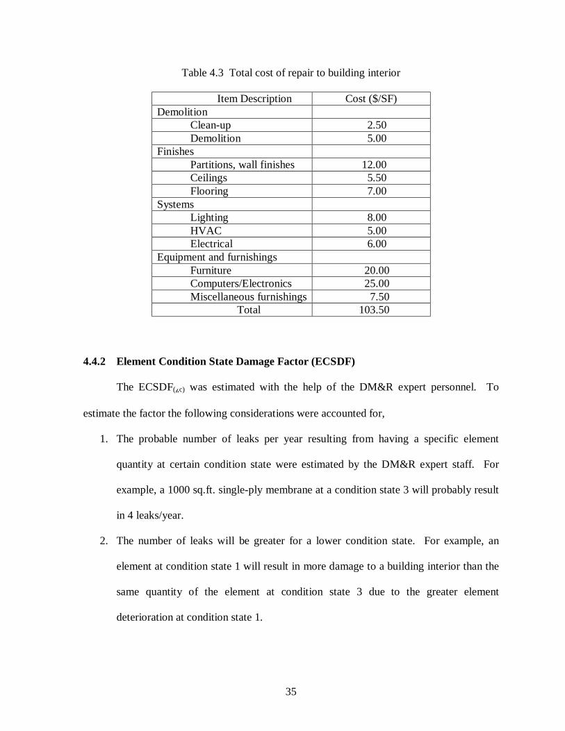
Table 4.3 Total cost of repair to building interior

Item Description Cost ($/SF) Demolition

Clean-up 2.50 Demolition 5.00

Finishes Partitions, wall finishes 12.00 Ceilings 5.50 Flooring 7.00

Systems Lighting 8.00 HVAC 5.00 Electrical 6.00

Equipment and furnishings Furniture 20.00 Computers/Electronics 25.00 Miscellaneous furnishings 7.50

Total 103.50

4.4.2 Element Condition State Damage Factor (ECSDF)

The ECSDF(l,c) was estimated with the help of the DM&R expert personnel. To

estimate the factor the following considerations were accounted for,

1. The probable number of leaks per year resulting from having a specific element

quantity at certain condition state were estimated by the DM&R expert staff. For

example, a 1000 sq.ft. single-ply membrane at a condition state 3 will probably result

in 4 leaks/year.

2. The number of leaks will be greater for a lower condition state. For example, an

element at condition state 1 will result in more damage to a building interior than the

same quantity of the element at condition state 3 due to the greater element

deterioration at condition state 1.

36

3. The area, in square feet of roof, affected by the leak resulting from a specific element

quantity at certain condition state was also an approximate estimate provided by the

experts working at the DM&R. For example, 1000 sq.ft. of single-ply membrane at a

condition state 3 will have about 4 leaks/year that will damage a total area of about 7

sq.ft. of building interior in each year.

The ECSDF(l,c) of an element (l) at an initial condition state (c) is the ratio of the

probable damaged area of the building interior to the quantity of the element at the condition

state.

ECSDF (l,c) = damage thecausing measureunit element ofQuantity

interior building damaged of Area (4.3)

Table 4.4 shows the element condition state, element unit measure causing the leak,

number of leaks caused by having the element unit measure at a certain condition state, and

the corresponding ECSDF of each element at each condition state.

4.5 Equivalent, Uniform Annual Cost Calculation for Maintenance Action

Alternatives

Three types of maintenance action alternatives are available for an element: do-

nothing, major maintenance, or replacement. This section describes the method used to

estimate the Equivalent, Uniform Annual Costs (EUAC(l,c,k)) of the alternatives. The

reductions in EUAC(l,c,k) that are associated with the optimum set of improvement

37

alternatives will be the objective function value. In addition, some minor routine

maintenance is performed for each element on an annual basis.

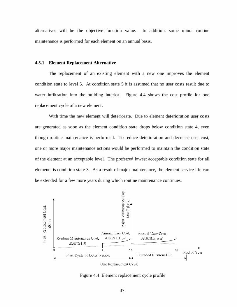
4.5.1 Element Replacement Alternative

The replacement of an existing element with a new one improves the element

condition state to level 5. At condition state 5 it is assumed that no user costs result due to

water infiltration into the building interior. Figure 4.4 shows the cost profile for one

replacement cycle of a new element.

With time the new element will deteriorate. Due to element deterioration user costs

are generated as soon as the element condition state drops below condition state 4, even

though routine maintenance is performed. To reduce deterioration and decrease user cost,

one or more major maintenance actions would be performed to maintain the condition state

of the element at an acceptable level. The preferred lowest acceptable condition state for all

elements is condition state 3. As a result of major maintenance, the element service life can

be extended for a few more years during which routine maintenance continues.

Figure 4.4 Element replacement cycle profile

38

Table 4.4 ECSDF calculation

Deteriorated/damaged Membrane- Useless/ non-functional 1 1000 13 39 0.04Infiltration of water in building- Damaged 2 1000 9 27 0.03Infiltration of water in roof system/ partially deteriorated- Deficient with no damage 3 1000 4 7 0.01

Loose/dry Membrane Lap or wrinkled/ridging Membrane/ slightly deteriorated- No deficiency

4 1000 0 0 0.00

New/excellent Membrane- New condition 5 1000 0 0 0.00Deteriorated/damaged Membrane- Useless/ non-functional 1 1000 13 39 0.04Infiltration of water in building- Damaged 2 1000 9 22 0.02Infiltration of water in roof system/ partially deteriorated- Deficient with no damage 3 1000 4 5 0.01

Loose/dry Membrane Lap or wrinkled/ridging Membrane/ slightly deteriorated- No deficiency 4 1000 0 0 0.00

New/excellent Membrane- New condition 5 1000 0 0 0.00Collapsed Insulation/ fully saturated- Useless/ non-functional 1 1000 0 3 0.00Large area of saturation- Damaged 2 1000 0 2 0.00

Small Area of saturation/ partially damaged- Deficient with no damage 3 1000 0 1 0.00

Shuffled/loose Insulation, loose Insulation fastener/ slightly damaged- No deficiency 4 1000 0 0 0.00

New/excellent Insulation- New condition 5 1000 0 0 0.00Dried/deteriorated Base Flashing- Useless/ non-functional 1 100 9 13 0.13Partially deteriorated /loose Base Flashing- Damaged 2 100 6 5 0.05Wide spread cracks- Deficiency with no damage 3 100 3 3 0.03Small hair-line cracks- Deterioration with no deficiency 4 100 0 0 0.00New/excellent Base Flashing- New condition 5 100 0 0 0.00

Multiple-ply membrane (SF)

Insulation (SF)

Single-ply base flashing (LF)

# Leak/yearDamage building

interior (SF) ECSDF

Single-ply membrane (SF)

Element Condition State Description CSElement unit

measure causing leak

39

Table 4.4 Continued

Dried/deteriorated Base Flashing- Useless/ non-functional 1 100 9 10 0.10Partially deteriorated /loose Base Flashing- Damaged 2 100 3 6 0.06Wide spread cracks- Deficiency with no damage 3 100 3 3 0.03Small hair-line cracks- Deterioration with no deficiency 4 100 0 0 0.00New/excellent Base Flashing- New condition 5 100 0 0 0.00Missing Counter Flashing- Useless/ non-functional 1 100 9 13 0.13Loose Counter Flashing/severely damaged- Damaged 2 100 4 5 0.05Partially deteriorated/damaged Counter Flashing- Deficiency with no damage

3 100 2 3 0.03

Slightly deteriorated/damaged/rusted Counter Flashing- No deficiency 4 100 0 0 0.00

New/excellent Counter Flashing condition 5 100 0 0 0.00Missing or ineffective Gutter/ useless/ non-functional 1 100 0 3 0.03

Substantially disconnected & leaking Gutter/ severely damaged- Damaged 2 100 0 2 0.02

Partially disconnected & leaking Gutter/partially damaged- Deficient with no damage

3 100 0 2 0.02

Slightly deteriorated/loose Gutter- No deficiency 4 100 0 0 0.00New/excellent Gutter- New condition 5 100 0 0 0.00Missing or ineffective Downspout- Useless/ non-functional 1 12 0 3 0.25Substantially disconnected/ clogged & leaking Downspout/ severely damaged- Damaged 2 12 0 2 0.17

Partially disconnected/ clogged & leaking Downspout/ partially damaged- Deficient with no damage

3 12 0 1 0.08

Slightly deteriorated/ clogged/loose Downspout- No deficiency 4 12 0 0 0.00New/excellent Downspout- New condition 5 12 0 0 0.00Missing Drain Strainer- Useless/ non-functional 1 2 0 3 1.50Deteriorated/damaged Drain Strainer- Damaged 2 2 0 2 1.00Fully clogged Drain Strainer/ partially deteriorated- Deficient with no damage 3 2 0 1 0.50

Partially clogged Drain Strainer/ slightly deteriorated/damaged- No deficiency

4 2 0 0 0.00

New/excellent Drain Strainer- New condition 5 2 0 0 0.00

Counter fashing (LF)

Gutter (LF)

Downspout (LF)

Drain strainer (EA)

Multiple-ply base flashing (LF)

40

Table 4.4 Continued

Unleveled Copping Cap Units-missing- Useless/ non-functional 1 100 9 7 0.07Masonry saturation & efflorescence- Damaged 2 100 4 5 0.05Failure of Copping Cap Bed Joint- Deficiency with no damage 3 100 2 4 0.04Failure of Copping Cap Head Joint- Deterioration with no deficiency 4 100 0 0 0.00New/excellent Copping Cap- New condition 5 100 0 0 0.00Missing Termination Bar- Useless/ non-functional 1 100 9 7 0.07Partially loose/ damaged Termination Bar- Damaged 2 100 4 3 0.03Partially loose but not damaged Termination Bar- Deficient with no damage 3 100 2 1 0.01

Slightly loose- No deficiency 4 100 0 0 0.00New/excellent Termination Bar- New condition 5 100 0 0 0.00Missing Edge Metal 1 100 10 20 0.20Deteriorated/damage Edge Metal 2 100 6 11 0.11Loose Edge Metal- Deficiency with no damage 3 100 3 3 0.03Slightly deteriorated Edge Metal- No deficiency 4 100 0 0 0.00New/excellent Edge Metal condition 5 100 0 0 0.00Missing Shingles- Useless/non-functional 1 100 4 3 0.03Loose/split Shingles- Damaged 2 100 2 2 0.02Partially deteriorated/damaged Shingles- Deficient with no damage 3 100 1 1 0.01Loose Shingle tabs/ buckled Shingles- No deficiency 4 100 0 0 0.00New/excellent Shingles- New condition 5 100 0 0 0.00Missing Slate- Useless/ non-functional 1 100 8 3 0.03Broken Slate- Damaged 2 100 4 2 0.02Loose Slate/ partially damaged- Deficient with no damage 3 100 2 1 0.01Slightly worn/aged Slate- No deficiency 4 100 0 0 0.00New/excellent Slate- New condition 5 100 0 0 0.00Missing Hip/Ridge Cap- Useless/ non-functional 1 100 1 3 0.03Deteriorated/damaged Hip/Ridge Cap- Damaged 2 100 1 2 0.02Slightly deteriorated Hip/Ridge Cap- Deficiency with no damage 3 100 1 1 0.01Worn/aged/rusted Hip/Ridge Cap - Deterioration with no deficiency 4 100 0 0 0.00New/excellent Hip/Ridge Cap - New condition 5 100 0 0 0.00

Slate (SF)

Hip/Ridge cap (LF)

Coping cap (LF)

Termination bar (LF)

Edge metal (LF)

Shingle (SF) (Asphalt)

41

The Replacement-Cycle Cost, RCC(l,c,k), of element (l) at a beginning condition state

(c) and final condition state 5 can be expressed as:

)n,r,F/P(*AUCST)n,r,F/P(*RMCST IRC RCCSL

tn)n,c,(

SL

0n)n,()(c,5),( ∑+∑+=

==llll

)m,r,F/P(*MMC )k,c,(l+ )zm,r,F/P(*MMC )k,c,( ++ l

)z2m,r,F/P(*MMC )k,c,( ++ l +………. (4.4)

where,

IRC(l) = Initial Replacement Cost of element (l),

RMCST(l,n) = Regular Maintenance Cost of element (l) at year (n),

MMC(l,c,k) = Major Maintenance Cost of element (l) at beginning condition state

(c) improved to final condition state (k),

AUCST(l,c,n) = Annual User Cost of element (l) at initial condition state (c) at year

(n),

SL = Expected Service Life of the element,

(P/F,r,n) = Single-payment present value factor; and

r = Nominal rate of return

z = m-t, from Figure 4.4

It is assumed that an element will always be replaced at the end of its service life,

because the element is assumed to be always required on the roof. The cost profile for

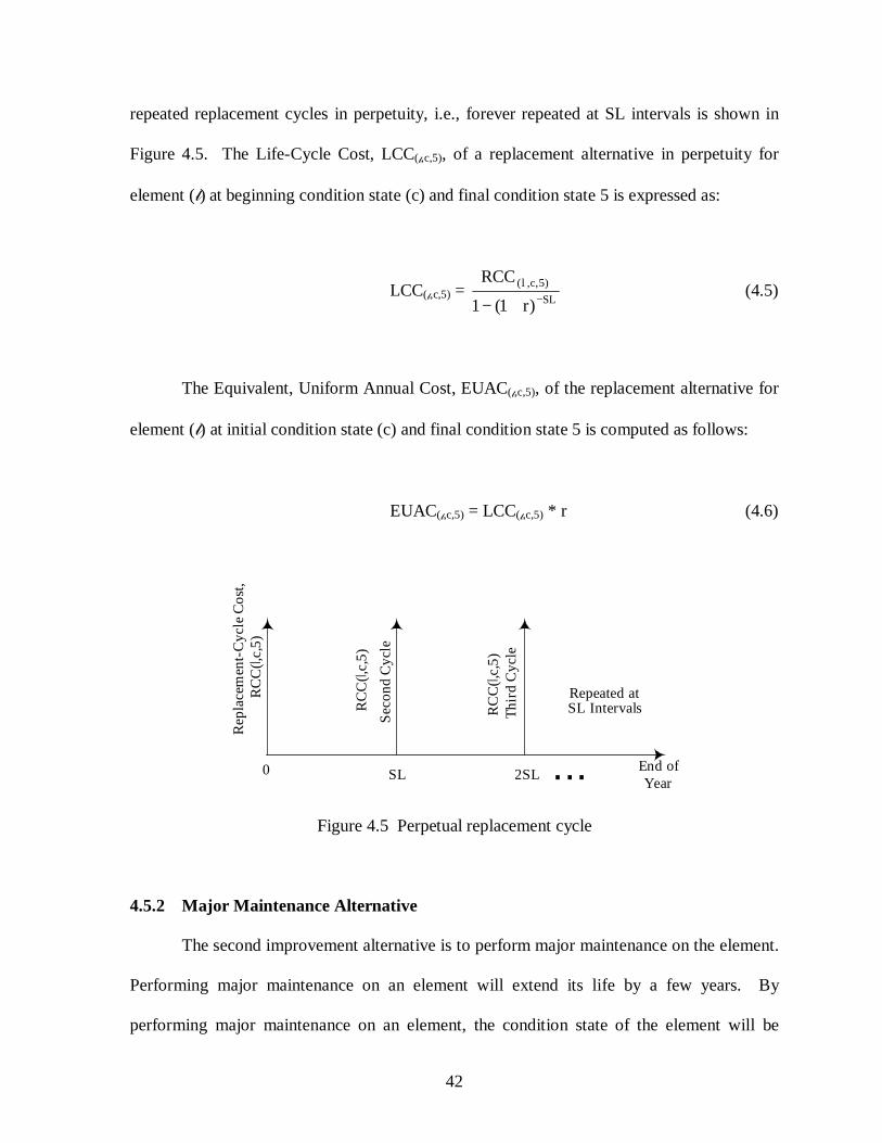
42

repeated replacement cycles in perpetuity, i.e., forever repeated at SL intervals is shown in

Figure 4.5. The Life-Cycle Cost, LCC(l,c,5), of a replacement alternative in perpetuity for

element (l) at beginning condition state (c) and final condition state 5 is expressed as:

LCC(l,c,5) = SL)5,c,(

)r1(1

RCC−+−

l (4.5)

The Equivalent, Uniform Annual Cost, EUAC(l,c,5), of the replacement alternative for

element (l) at initial condition state (c) and final condition state 5 is computed as follows:

EUAC(l,c,5) = LCC(l,c,5) * r (4.6)

0

Rep

lace

men

t-C

ycle

Cos

t,R

CC

(l,c,

5)

End ofYear

Seco

nd C

ycle

SL 2SL

Thir

d C

ycle

Repeated atSL Intervals

...

RC

C(l,

c,5)

RC

C(l,

c,5)

Figure 4.5 Perpetual replacement cycle

4.5.2 Major Maintenance Alternative

The second improvement alternative is to perform major maintenance on the element.

Performing major maintenance on an element will extend its life by a few years. By

performing major maintenance on an element, the condition state of the element will be

43

raised to a higher condition state. Thus, the extension in the element life will be equal to the

number of years an element stays at the new condition state before dropping to a lower

condition state. The number of years which an element stays in a condition state before

dropping to a lower condition state was defined in Section 4.1.1 as the average condition

state service life. At the end of the extended life, the element will be replaced by a new one.

The cost profile for a major maintenance cycle of an existing element followed by

replacement is shown in Figure 4.6.

The Life-Cycle Cost, LCC(l,c,k), of a major maintenance alternative in perpetuity for

element (l) at an initial condition state (c), and final condition state (k) is expressed as:

LCC(l,c,k) = MMC(l,c,k) )n,r,F/P(*AUCST)n,r,F/P(*RMCST Ex

0n)n,c,(

Ex

0n)n,( ∑+∑+

==ll

+ LCC(l,c,5) * (P/F, r, Ex) (4.7)

where,

MMC(l,c,k) = Major Maintenance Cost for element (l) at initial condition state

(c) and final condition state (k); and

Ex = Extended element life of element (l) due to major maintenance.

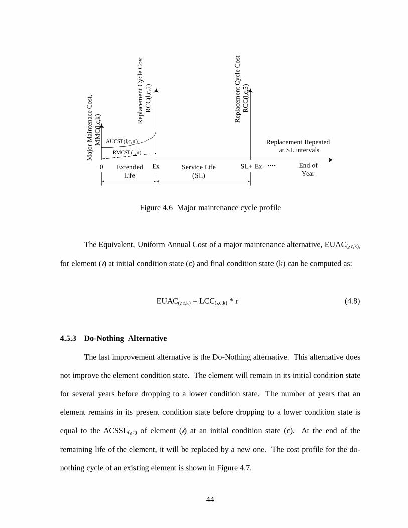
44

0 ....Ex Service Life(SL)

Maj

or M

aint

enac

e C

ost,

MM

C(l,

c,k)

End ofYear

ExtendedLife

SL+ Ex

Replacement Repeatedat SL intervals

Rep

lace

men

t Cyc

le C

ost

RC

C(l,

c,5)

Rep

lace

men

t Cyc

le C

ost

RC

C(l,

c,5)

RMCST ( l,n)

AUCST( l,c,n)

Figure 4.6 Major maintenance cycle profile

The Equivalent, Uniform Annual Cost of a major maintenance alternative, EUAC(l,c,k),

for element (l) at initial condition state (c) and final condition state (k) can be computed as:

EUAC(l,c,k) = LCC(l,c,k) * r (4.8)

4.5.3 Do-Nothing Alternative

The last improvement alternative is the Do-Nothing alternative. This alternative does

not improve the element condition state. The element will remain in its initial condition state

for several years before dropping to a lower condition state. The number of years that an

element remains in its present condition state before dropping to a lower condition state is

equal to the ACSSL(l,c) of element (l) at an initial condition state (c). At the end of the

remaining life of the element, it will be replaced by a new one. The cost profile for the do-

nothing cycle of an existing element is shown in Figure 4.7.

45

0 ....R Service Life(SL)

End ofYear

RemainningLife

SL+ R

Replacement Repeatedat SL intervals

Rep

lace

men

t Cyc

le C

ost

RC

C(l,

c,5)

Rep

lace

men

t Cyc

le C

ost

RC

C(l,

c,5)

RMCST ( l,n)

AUCST( l,c,n)

Figure 4.7 Do-nothing cycle profile

The Life-Cycle Cost, LCC(l,c,c-1), of a major maintenance alternative in perpetuity for

element (l) at an initial condition state (c), and final condition state (c-1) is expressed as:

LCC(l,c,c-1) = )n,r,F/P(*AUCST)n,r,F/P(*RMCST R

0n)n,c,(

R

0n)n,( ∑+∑

==ll

+ LCC(l,c,5) * (P/F, r, R) (4.9)

The Equivalent, Uniform Annual Cost of a do-nothing alternative, EUAC(l,c,c-1), for

element (l) at initial condition state (c) and final condition state (c-1) can be computed as:

EUAC(l,c,c-1) = LCC(l ,c,c-1) * r

(4.10)

46

4.6 Reduction in Equivalent Uniform Annual Costs

Maximizing the total amount of reductions in annual cost will assure the optimal

maintenance solution for all roof elements available under budgetary constraint.

To optimize roof maintenance, the Reduction in Equivalent Uniform Annual Costs,

REUAC(i,j,l,c,k) for all maintenance alternatives that are possible for each roof element (l) at

initial condition state (c) and final condition state (k) has to be calculated. REUAC(i,j,l,c,k)

calculates the saving in annual cost associated with a specific alternative.

The REUAC(i,j,l,c,k) for building (i), section (j), element (l) at initial condition state (c)

and final condition state (k) is calculated as follows:

REUAC(i,j,l,c,k) = AUCST(l,c) – EUAC(i,j,l,c,k)

(4.11)

As an example, assume an element is at condition state 2 and the possible

maintenance alternatives are: do-nothing or replace the element with a new one. The do-

nothing alternative is to leave the element at its current condition state, CS= 2, while the

replacement alternative is to improve the element condition state to CS= 5 by replacing the

element with a new one. The following hypothetical values are available as an example:

AUCST(l,c) EUAC(i,j,l,c,k) REUAC(i,j,l,c,k)($) ($) ($)

Do-nothing 55.95 223.50Replacement 39.99 239.46

Alternative

279.45

47

To maximize the saving in annual cost, it is necessary to maximize the total amount

of reductions in equivalent uniform annual cost. For the previous example, the replacement

alternative would be chosen under budgetary constraint. Minimizing EUAC(i,j,l,c,k) or

AUCST(l,c) in isolation will not produce the optimal solution. The reason for including

AUCST(l,c) in the calculation of the REUAC(i,j,l,c,k) is because building users are the ultimate

owners of the buildings.

4.7 Reduction in Re-roofing Uniform Annual Costs

Maximizing the total amount of reductions in re-roofing annual cost will ensure the

optimal maintenance solution for all roof sections under budgetary constraint. To optimize

roof maintenance, the Re-roofing Uniform Annual Cost, RFUAC(s) for each section (s) has to

be calculated. RRFUAC(s) is the saving in annual cost due to choosing re-roofing the roof

section. The RRFUAC(s) for section (s) is calculated as follows:

RRFUAC(s) = MCST(s) – RFUAC(s) (4.12)

where,

MCST(s) = Total maintenance cost of section (s) resulting from maximizing

REUAC(i,j,l,c,k)

RFUAC(s) = Re-roofing Uniform Annual Cost of section (s) calculated using the

following equation,

RFUAC(s) = RCST(s))()1(1 sSLr

r−+−

(4.13)

where,

48

RCST(s)= Re-roofing cost of section (s)

As an example, assume that total maintenance cost of section (1) equals $ 300, while

the total maintenance cost of section (2) equals $2500. If the RFUAC for both sections (1)

and (2) equals $500, then the RRFUAC equals -$200 for section (1) and $2000 for section

(2). The model will choose section (2) for re-roofing while maintenance work is performed

on roof section (1). This is all performed under a budget restriction.

4.8 Projection of Future Element Condition State

Element condition deteriorates with time. The finite Markov Chain class will be used

to project the quantity of each element at each condition state for the subsequent analysis

year. A Markov chain is a discrete-state random process in which the evolution of the state

of the process beginning at a time (t) depends only on the current state X(t), and not how the

chain reached its current state or how long it has been in that state. Therefore, a finite

Markov chain will be used since the condition states that a roof element may be in are

considered to be discrete and countable and the probability that an element will transition

from condition state (c) to condition state (k) does not depend on how the (c) state was

arrived at. This means that the current state will always be considered as the starting point

because the time between state changes is a random variable with a memory-less distribution.

The construction of a Markov chain requires two basic parts, an initial distribution and a

transition matrix.

49

4.8.1 Initial Distribution

Each element is given an ACSSL at each CS. Assuming that the life of an element at

any CS is exponentially distributed, knowledge of the ACSSL identifies the distribution of

the life of the element, which shall be denoted by the random variable Yc, in state (c) as:

=)(tfcY

cµ1 cµ

-t

e (4.14)

Assuming that the deterioration in the element CS leads to the next lower CS (and no

to other state) then the probability of the element remaining at the same CS for one year is

given by the probability that it will survive longer than one year in that state,

∫∞

=

−−

==≥=1

11)1Pr(

t

t

cccc

cc edteYp µµ

µ (4.15)

and the probability that one element will deteriorate to CS (c-1) is

cccc pp −=− 11 , c= 5,4,3,2 (4.16)

while,

111 =p (4.17)

This means that an element reaching a failure condition state, CS=1, will remain in

that condition state forever if no maintenance action is performed.

50

4.8.2 Transition Matrix

Based on the ACSSL defined in Table 4.1 for each element at each CS, and the

assumption that the deterioration in an element CS leads to the next lower CS (and no to

other state), a one year transition probability matrix P is constructed as follows:

P =

−−

−−

100001000

010000100001

2222

3333

4444

5555

PPPP

PPPP

where,

Pcc = Probability of a condition state c quantity staying in state c after one year,

c = 2,3,4,5, and

P11 = 1, because we have only 5 condition states; therefore, an element deteriorates to

condition state 1 and remains at condition state 1 with no further deterioration.

The probabilities (Pcc) of all elements remaining at their initial condition state (c)

more than one year are given in Table 4.5. It should be noted that, for the sake of brevity, the

probabilities in the table are written for only two significant figures. However, the full

accuracy of the exponentiation operation was retained throughout the calculations.

As an example consider the do-nothing maintenance action. The element will

continuously deteriorate year after year until it reaches CS = 1, where it stays forever. Let

X(t) denote the vector of the CS of the element at the start of year t; given in its expanded

form as

51

X(t) = (x5(t), x4(t), x3(t), x2(t), x1(t)) , t = 1, 2, 3, …..

The starting CS in the first year is denoted by X(0) and is given by

X(0) = (1,0,0,0,0),

This means that the entire element quantity is at CS = 5. Clearly,

X(1) = X(0) P,

which can be written in an expanded form as follows:

(x5(1), x4(1), x3(1), x2(1), x1(1))

= (x5(0), x4(0), x3(0), x2(0), x1(0))

−−

−−

100001000

010000100001

2222

3333

4444

5555

PPPP

PPPP

= (P55, 1-P55, 0, 0, 0)

So generally,

X(t) = X(t-1) P

Substituting for X(t-1) = X(t-2) P one gets

X(t) = [X(t-1) P] P = X(t-1) 2P

Continuing recursively all the way we secure,

52

X(t) = X(0) tP

So to calculate the distribution of an element after year t, the transition matrix P is

raised to the tht power and pre-multiplied by the original state X(0).

Table 4.5 Transition probability for maintenance element

No. Element CS ACSSL Pck5 13 0.934 5 0.823 2 0.612 1 0.371 0 1.005 18 0.954 6 0.853 1.5 0.512 0.75 0.261 0 1.005 15.5 0.944 4.5 0.803 2 0.612 0.75 0.261 0 1.005 10 0.904 5 0.823 2 0.612 1.25 0.451 0 1.005 12.5 0.924 6 0.853 3 0.722 2 0.611 0 1.005 5.5 0.834 4 0.77883 3.5 0.752 2 0.60651 0 1.005 5 0.824 3 0.723 2 0.612 0.75 0.261 0 1.00

7 Gutter


Single-ply membrane

6

5

4

3

2

1

Counter Flashing

Base Flashing Multiple-ply

Base Flashing Single-ply

Insulation

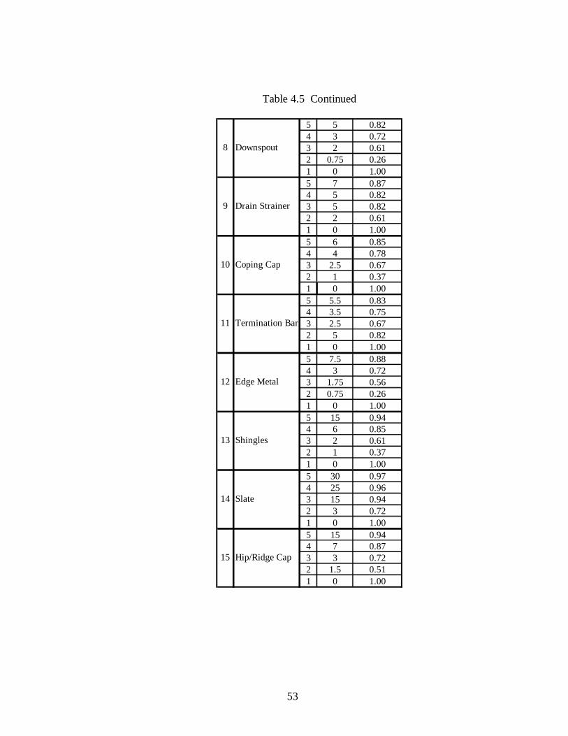
53

Table 4.5 Continued

5 5 0.824 3 0.723 2 0.612 0.75 0.261 0 1.005 7 0.874 5 0.823 5 0.822 2 0.611 0 1.005 6 0.854 4 0.783 2.5 0.672 1 0.371 0 1.005 5.5 0.834 3.5 0.753 2.5 0.672 5 0.821 0 1.005 7.5 0.884 3 0.723 1.75 0.562 0.75 0.261 0 1.005 15 0.944 6 0.853 2 0.612 1 0.371 0 1.005 30 0.974 25 0.963 15 0.942 3 0.721 0 1.005 15 0.944 7 0.873 3 0.722 1.5 0.511 0 1.00

15

14

13

Hip/Ridge Cap

Slate

Shingles

8

Edge Metal

Termination Bar

Coping Cap

Drain Strainer

Downspout

12

11

10

9

54

4.9 Optimization Model

Two optimization models will be used in this study. The first optimization

maximizes the saving in annual cost by maximizing the total amount of reduction in

equivalent uniform annual cost. The second optimization also maximizes the saving in

annual cost by maximizing the total amount of reduction in annual re-roofing cost.

4.9.1 Maximizing Total Amount of Reduction in EUAC

After quantifying the REUAC and MAUCST for each maintenance alternative of

each roof element, a binary linear programming approach was used to optimize the selection

of maintenance actions to perform on each roof element under a limited budget. The

following model was used:

Objective function:

Max ∑∑∑∑ ∑= = = = −=

28

1

12

1

15

1

5

1

5

1),,,,(),,,,(),,,,( **

i j c ckkcjikcjikcji REUACQtyX

llll (4.18)

Subject to:

Constraint 1:

28 12 15 5 5

( , , , , ) ( , , , , ) ( , , , , )1 1 1 1 1

* *i j c k i j c k i j c ki j c k c

X Qty MAUCST BUDGET= = = = = −

≤∑∑∑∑ ∑ l l ll

(4.19)

Constraint 2:

5

( , , , , )1

1i j c kk c

X= −

=∑ l , ∀ i,j,l values, c = 1, 2, …, 5 (4.20)

55

Constraint 3:

X(i,j,l,,c,k) = 0 or 1 (4.21)

where,

BUDGET = Available maintenance budget

i = Building number

j = Roof section

l = Maintenance element

c = Element condition state before maintenance

k = Element condition state after maintenance

X(i,j,l,c,k) = Decision variable for building (i), roof section (j), element (l), initial

condition state (c), and final condition state (k)

The model will compute the maintenance actions performed on each roof element that

will maximize the total savings in annual cost within the available budget. For each element

on each roof section of each building, there is only one decision variable X(i,j,l,c,k) which will

have a value of 1. This means that for each element (l) the model will select one

maintenance action that will improve the element from condition state (c) to condition state

(k) and maximize the total savings.

The benefits are calculated as the saving in future replacement costs due to applying

the maintenance action on the element. After obtaining the recommended maintenance action

on each element, the condition state of the elements is updated. The quantity of elements

improving to a better condition state and the quantity of elements deteriorating to a worst

56

condition state will be calculated and the resulting element condition state will help in

creating the inputs for the following year analysis.

4.9.2 Maximizing Total Amount of Reduction in Re-roofing Costs

After maximizing the total reduction in EUAC, another optimization is performed to

ensure that the total cost of maintenance actions performed on a roof section does not exceed

the cost of re-roofing the section. The 28 buildings available for this study include a total of

116 roof sections. A binary linear programming approach was used to optimize the decision

of maintaining or re-roofing a roof section. The following model was used:

Objective function:

Max 116

( ) ( )1

*s ss

X RRFUAC=

∑ (4.22)

Subject to:

Constraint 1:

116

( ) ( )1

*s ss

X RCST RBUDGET=

≤∑ (4.23)

Constraint 2:

X(s) = 0 or 1 (4.24)

where,

RBUDGET = Available re-roofing budget

s = Roof section

57

5. INVENTORY, CONDITION AND COST DATA

This chapter presents input data required to run the optimization model. The data was

obtained from or developed with the assistance of the Department of Maintenance and Repair

(DM&R) at North Carolina State University.

5.1 Number of Buildings and Buildings Roof Sections

The North Carolina State University campus has an inventory of the 128 buildings.

Inspections of these buildings are performed biennially and the repairs performed on each

building are stored in the department data base.

For the purpose of this model application, only 28 buildings were chosen because of

the availability of data on their roof elements. Each building roof is divided into one or more

sections. The division of roof buildings into sections is based on the variation in roof

elevation or on the use of different roofing material, and in some cases, it is based on both.

Table 5.1 lists the 28 buildings and the number of sections associated with each building.

5.2 Number of Maintenance Elements

DM&R defines 15 roof elements in its database. The following is a list of these

maintenance elements:

1- Hip/Ridge Cap 2- Coping Cap 3- Base Flashing 4- Edge Metal 5- Counter Flashing 6- Shingle

58

7- Slate 8- Gutter 9- Downspout 10- Drain Strainer 11- Membrane 12- Insulation 13- Termination Bar 14- Scupper 15- Penetration Flashing

Table 5.1 Building name and number of sections associated

Building Name Number of Sections Alumini Memorial Building 3 D.H.Hill Library 4 Harris Hall 1 Pullen Hall 1 West Dunn Building 2 Winston Hall 6 Head House Unit 2 1 Hillsborough Building 2 Hodges Wood Products Lab 2 Jordan Hall 10 Page Hall 1 Peele Hall 1 Phytotron 5 Pulp and Paper Labs 7 Thompkins Hall 3 Williams Hall 12 Withers Hall 3 Administrative Services 2 Avent Ferry Convention Ctr 5 Biltmore Hall 4 Bostian Hall 6 Bureau of Mines 1 Caldwell Hall 5 Cates Avenue Steam Plant 5 Daniels Hall 8 Don E. Ellis Lab 2 Gardner Hall 12 Harrelson Hall 2

59

For the purpose of this model application, two elements were removed from the

previous list. One removed element is the scupper; it was removed because no maintenance

action is performed on it and it does not affect the roof maintenance cost. Penetration

flashing was also removed because there were no available data in the DM&R database.

Because of the important role penetration flashing plays in preventing water infiltration at

roof projections, an approximate quantity was calculated and added to the base flashing

quantity of each roof section.

Another modification was done to the maintenance element list. The membrane and base

flashing were subdivided into single-ply and multiple-ply types. This subdivision allowed

deterioration rates and maintenance costs of these materials to be better represented. No

subdivision was needed for the rest of the elements due to the similarity in the average

deterioration rates and maintenance costs for the material types encountered within each.

When the optimization model was first executed it was noted that the condition state

weighted average of insulation sometimes improved when the membrane did not. This was

logically impossible because the insulation can not be replaced or fixed without replacing the

membrane. To solve this problem, the insulation was left in the model but was given zero

quantities and half of the insulation maintenance cost was added to the cost of membrane

maintenance. This assures that the insulation would be repaired or replaced over 50% of the

area of membrane maintenance or replacement. Table 5.2 shows the modified list of the

maintenance elements.

60

Table 5.2 Maintenance element and corresponding unit measure

Maintenance element Unit measure Single-ply membrane Sq. Ft. Multiple-ply membrane Sq. Ft. Insulation Sq. Ft. Single-ply base flashing Linear Ft. Multiple-ply base flashing Linear Ft. Counter flashing Linear Ft. Gutter Linear Ft. Downspout Linear Ft. Drain strainer Each Coping cap Linear Ft. Termination bar Linear Ft. Edge metal Linear Ft. Shingle Sq. Ft. Slate Sq. Ft. Hip/Ridge cap Linear Ft.

5.3 Quantity of Maintenance Elements at Each Condition State

The quantity of maintenance elements and their distribution among different

condition states are important factors in determining the annual cost of performing

maintenance. They also have an important role in the optimization model because costs and

benefits of the decisions increase and decrease with the increase or decrease in the quantity

and present condition of units maintained.

The records in the DM&R database are kept for each roof section. The data available

of interest to the research consists of the total square feet area and the perimeter length of

each roof section. The types of repairs to be performed on each element and the quantity of

element to be repaired are also available in the DM&R database. The availability of the this

information helped in developing the allocation of element quantities among the different

61

condition states. Table 5.3 shows Harris Hall, Pullen Hall, and West Dunn building element

quantities distributed over their condition states. A table showing all buildings element

initial quantities distributed over their condition states is available in Appendix A3.

5.4 Real Rate of Return

The interest rate should reflect the time value of money. It is used to convert costs

occurring at different future times to equivalent costs at a common point in time. There are

two main types of Interest rates; nominal and real. The nominal interest rate includes general

price inflation, while the real interest rate, called also the Real Rate of Return (RRR), the net

of price inflation. The nominal rate of return is calculated as follows,

Nominal rate of return = RRR + (1 + RRR) f (5.1)

where,

f = Inflation rate

For computational simplicity, inflation will be set to zero and the nominal rate of

return will equal the RRR. Thus, for this analysis, the budgets are estimated in today’s

dollar.

62

Table 5.3 Examples of element quantity distribution over different condition states

Single-ply membrane

(SF)


(SF)

Insulation (SF)

Single-ply base

flashing (LF)

Multiple-ply base flashing

(LF)

Counter flashing

(LF)

Gutter (LF)

Downspout (LF)

Drain strainer (EA)

Coping cap (LF)


Edge metal (LF)

Shingle (SF)

Slate (SF)

Hip/Ridge cap (LF)

1 0.0 0.0 0.0 0.0 0.0 0.0 0.0 0.0 0.0 0.0 0.0 0.0 0.0 0.0 0.02 0.0 0.0 0.0 0.0 0.0 0.0 0.0 0.0 0.0 0.0 0.0 0.0 0.0 0.0 0.03 0.0 0.0 0.0 0.0 0.0 0.0 0.0 0.0 0.0 0.0 0.0 0.0 0.0 0.0 0.04 0.0 0.0 0.0 0.0 0.0 0.0 0.0 0.0 0.0 0.0 0.0 0.0 0.0 0.0 0.05 0.0 0.0 0.0 239.7 0.0 239.7 239.7 0.0 0.0 0.0 0.0 239.7 4871.0 0.0 0.01 0.0 0.0 0.0 0.0 0.0 0.0 0.0 0.0 0.0 0.0 0.0 0.0 0.0 0.0 0.02 0.0 0.0 0.0 0.0 0.0 0.0 0.0 0.0 0.0 0.0 0.0 0.0 0.0 0.0 0.03 0.0 0.0 0.0 0.0 0.0 0.0 0.0 0.0 0.0 0.0 0.0 0.0 0.0 0.0 0.04 0.0 0.0 0.0 0.0 0.0 77.3 0.0 0.0 1.0 0.0 0.0 20.0 0.0 0.0 0.05 2207.0 0.0 0.0 154.7 0.0 77.3 0.0 0.0 3.0 0.0 0.0 134.7 0.0 0.0 0.01 0.0 0.0 0.0 0.0 0.0 0.0 0.0 0.0 0.0 0.0 0.0 0.0 0.0 0.0 0.02 0.0 0.0 0.0 0.0 0.0 0.0 0.0 0.0 0.0 0.0 0.0 0.0 0.0 0.0 0.03 0.0 0.0 0.0 0.0 0.0 4.0 0.0 0.0 0.0 0.0 0.0 0.0 0.0 0.0 0.04 0.0 0.0 0.0 0.0 0.0 23.9 0.0 36.0 0.0 15.0 56.9 0.0 0.0 0.0 0.05 368.0 0.0 0.0 75.8 0.0 47.9 0.0 0.0 0.0 60.8 19.0 0.0 0.0 0.0 0.01 0.0 0.0 0.0 0.0 0.0 0.0 0.0 0.0 0.0 0.0 0.0 0.0 0.0 0.0 0.02 0.0 0.0 0.0 0.0 0.0 0.0 0.0 0.0 0.0 0.0 0.0 0.0 0.0 0.0 0.03 0.0 0.0 0.0 0.0 0.0 0.0 0.0 0.0 0.0 0.0 0.0 98.6 0.0 0.0 0.04 429.0 0.0 0.0 0.0 0.0 0.0 98.6 24.0 0.0 0.0 0.0 0.0 0.0 0.0 0.05 0.0 0.0 0.0 0.0 0.0 0.0 0.0 0.0 0.0 0.0 0.0 0.0 0.0 0.0 0.01 0.0 0.0 0.0 0.0 0.0 0.0 0.0 0.0 0.0 0.0 0.0 0.0 0.0 0.0 0.02 0.0 0.0 0.0 0.0 0.0 0.0 0.0 0.0 0.0 0.0 0.0 0.0 0.0 0.0 0.03 0.0 0.0 0.0 0.0 0.0 0.0 0.0 0.0 0.0 0.0 0.0 191.0 0.0 0.0 0.04 3129.0 0.0 0.0 235.3 0.0 235.3 235.3 24.0 0.0 0.0 0.0 44.3 0.0 0.0 0.05 0.0 0.0 0.0 0.0 0.0 0.0 0.0 0.0 0.0 0.0 0.0 0.0 0.0 0.0 0.01 0.0 0.0 0.0 0.0 0.0 0.0 0.0 0.0 0.0 0.0 0.0 0.0 0.0 0.0 0.02 0.0 0.0 0.0 0.0 0.0 0.0 0.0 0.0 0.0 0.0 0.0 0.0 0.0 0.0 0.03 0.0 0.0 0.0 0.0 0.0 0.0 0.0 0.0 0.0 0.0 0.0 573.0 0.0 0.0 0.04 15876.0 0.0 0.0 573.0 0.0 573.0 0.0 0.0 0.0 0.0 0.0 0.0 0.0 0.0 0.05 0.0 0.0 0.0 0.0 0.0 0.0 0.0 0.0 0.0 0.0 0.0 0.0 0.0 0.0 0.01 0.0 0.0 0.0 0.0 0.0 0.0 0.0 0.0 0.0 0.0 0.0 0.0 0.0 0.0 0.02 0.0 0.0 0.0 0.0 0.0 0.0 0.0 0.0 0.0 0.0 0.0 0.0 0.0 0.0 0.03 0.0 0.0 0.0 0.0 0.0 0.0 0.0 0.0 0.0 0.0 0.0 0.0 0.0 0.0 0.04 260.0 0.0 0.0 577.6 0.0 0.0 0.0 0.0 0.0 0.0 0.0 577.6 0.0 0.0 0.05 0.0 0.0 0.0 0.0 0.0 0.0 0.0 0.0 0.0 0.0 0.0 0.0 0.0 0.0 0.0

D.H.Hill Library

A1

A2

A3

A4

Alumini Memorial Building

A

B

C

Building Section CS

Maintenance Elements

63

5.5 Average Condition State Service Life

The average condition state service life is an important factor in determining its

service life and in calculating its life-cycle cost. In addition, the average condition state

service life determines the frequency in which major maintenance is performed on different

elements. The average condition state service life for each element at each condition state

was estimated by the roof maintenance personnel at the DM&R. For the elements used in

this study, Table 5.4 provides the average condition state service life values which are the

average times the elements will remain at a condition state without maintenance before

deteriorating to a lower condition state.

Table 5.4 Average condition state service life for each element at each condition state

Average condition state service life (years) Maintenance Element

5 4 3 2 1 Single-ply membrane 13.00 5.00 2.00 1.00 - Multiple-ply membrane 18.00 6.00 1.50 0.75 - Insulation 15.50 4.50 2.00 0.75 - Single-ply base flashing 10.00 5.00 2.00 1.25 - Multiple-ply base flashing 12.50 6.00 3.00 2.00 - Counter flashing 5.50 4.00 3.50 2.00 - Gutter 5.00 3.00 2.00 0.75 - Downspout 5.00 3.00 2.00 0.75 - Drain strainer 7.00 5.00 5.00 2.00 - Coping cap 6.00 4.00 2.50 1.00 - Termination bar 5.50 3.50 2.50 5.00 - Edge metal 7.50 3.00 1.75 0.75 - Shingle 15.00 6.00 2.00 1.00 - Slate 30.00 25.00 15.00 3.00 - Hip/Ridge cap 15.00 7.00 3.00 1.50 -

64

5.6 Unit Cost of Maintenance Actions

The unit cost of maintenance work performed on each roof element can be obtained

from North Carolina State University historical cost data or the Means Building Construction

Cost Data [16]. Since the maintenance costs required in this study are those incurred to

improve the roof element from a lower condition state to a higher one, a group of experts at

DM&R were asked to give their estimate of maintenance cost at each condition state for all

elements and the corresponding improvement resulting from the performed maintenance.

The group used their knowledge and the available data in the database. The individuals in

the group were allowed to discuss their estimates to reach an agreement on the proper

estimate for each element at each condition state. The results of this process are presented in

Appendix A1.

5.7 Equivalent Uniform Annual Cost

The Equivalent Uniform Annual Cost is calculated to estimate the savings in annual

costs resulting from performing a maintenance action. The EUAC is calculated for each

maintenance action performed on each maintenance element at each condition state. The

calculation of EUAC is discussed in detail in section 4.5. The values of all EUAC

maintenance action alternatives calculated for all elements are available in Appendix A2.

65

6. MODEL DEVELOPMENT

Two software programs, Excel and AMPL, were used for the optimization analysis.

Microsoft Excel is a spreadsheet program, while AMPL is an optimization program that uses

algebraic modeling language to solve linear, nonlinear and integer programming problems.

Excel operates on a MS Windows PC and AMPL operates on a SUN microcomputer

platform.

This chapter will present the use of the two programs to perform the optimization and

analysis. The chapter will also present two different approaches for optimizing roof

maintenance and replacement.

6.1 Optimizing Roof Maintenance Using Separated and Combined Budgets

Currently, the DM&R has two budgets. The first budget is used to perform

maintenance activity on university building roof elements. Maintenance work is performed

by department maintenance personnel, and consists of repairing or replacing roof elements.

The second budget available to the department is a capital budget which is used to perform

re-roofing of a building roof section. Re-roofing replaces all roof section elements.

Contractors usually perform the re-roofing work. If these two total budgets for all university

building roofs are apportioned on the basis of sq.ft. of roof, the amounts for the 28 buildings

in this study are $54,000 for maintenance activity and $246,000 for the re-roofing capital

budget. Two approaches will be considered, one based on separated budget amounts and a

second based on the combined budget amount.

66

In the separated budget approach, two optimizations are performed using the two

separate budgets. First optimization is performed to select the optimum maintenance action

on each roof element using the $54,000 budget. The total maintenance costs for each roof

section resulting from the first optimization are added and compared and the cost of

performing re-roofing on the section. Second, optimization is performed by maximizing the

difference between the total costs of performing maintenance work and the cost of re-roofing

the roof section using capital budget.

In the combined budget approach, the two budgets available are combined and used

to perform one optimization. The optimization will select the optimum maintenance or

replacement action on each roof element using the combined budget of $300,000. For both

approaches, separated and combined, Excel is used for data entry and performing certain

analysis, while AMPL performs the optimization.

6.2 Excel Operations

Excel was used to tabulate the input data, create the optimization model in algebraic

language, save the created model in a text file readable to AMPL, and use the optimized

results generated by AMPL to complete the analysis. An Excel file containing multiple

sheets was developed for this purpose.

The initial quantities obtained from the DM&R database are entered in the “Initial

Quantity” data sheet. Each element quantity entered at a specific condition state in the

“Initial Quantity” sheet, Table 6.1, will then be displayed in the fifth column of the “Initial

Building Data” sheet, Table 6.2. The entered quantity in “Initial Quantity” sheet will appear

in more than one cell in the “Initial Building Data” sheet depending on the maintenance

67

actions available for the specific condition state. If, for example, 15 LF of coping cap at

condition state 4 is entered for Alumini Memorial Building roof section C, Table 6.1, the

quantity will appear in the “Initial Building Data” sheet at condition state 43, 44, and 45,

Table 6.2. This means that the possible maintenance action for the 15 LF coping cap at

condition 4 are do nothing, 43 and 44, or replace the element, 45.

Other data entered into the “Initial Building Data” sheet are EUAC, ECSDF, Damage

cost, and MAUCST. The values displayed in these columns are obtained from different

sheets used to perform the calculations.

The “Initial Building Data” sheet will also be used to create the optimization model

only for the first year of the analysis horizon that has a total of 15 years. Table 6.2 shows a

sample of the data entered into the “Initial Building Data” sheet for building 1, section 3 and

elements 10 and 11. Table 6.3 describes the content of each column in Table 6.2.

68

Table 6.1 “Initial Quantity” data sheet

Single-ply membrane

(SF)


(SF)

Insulation (SF)

Single-ply base

flashing (LF)

Multiple-ply base flashing

(LF)

Counter flashing

(LF)

Gutter (LF)

Downspout (LF)

Drain strainer (EA)

Coping cap (LF)


Edge metal (LF)

Shingle (SF)

Slate (SF)

Hip/Ridge cap (LF)

1 0.0 0.0 0.0 0.0 0.0 0.0 0.0 0.0 0.0 0.0 0.0 0.0 0.0 0.0 0.02 0.0 0.0 0.0 0.0 0.0 0.0 0.0 0.0 0.0 0.0 0.0 0.0 0.0 0.0 0.03 0.0 0.0 0.0 0.0 0.0 0.0 0.0 0.0 0.0 0.0 0.0 0.0 0.0 0.0 0.04 0.0 0.0 0.0 0.0 0.0 0.0 0.0 0.0 0.0 0.0 0.0 0.0 0.0 0.0 0.05 0.0 0.0 0.0 239.7 0.0 239.7 239.7 0.0 0.0 0.0 0.0 239.7 4871.0 0.0 0.0

1 0.0 0.0 0.0 0.0 0.0 0.0 0.0 0.0 0.0 0.0 0.0 0.0 0.0 0.0 0.02 0.0 0.0 0.0 0.0 0.0 0.0 0.0 0.0 0.0 0.0 0.0 0.0 0.0 0.0 0.03 0.0 0.0 0.0 0.0 0.0 0.0 0.0 0.0 0.0 0.0 0.0 0.0 0.0 0.0 0.04 0.0 0.0 0.0 0.0 0.0 77.3 0.0 0.0 1.0 0.0 0.0 20.0 0.0 0.0 0.05 2207.0 0.0 0.0 154.7 0.0 77.3 0.0 0.0 3.0 0.0 0.0 134.7 0.0 0.0 0.01 0.0 0.0 0.0 0.0 0.0 0.0 0.0 0.0 0.0 0.0 0.0 0.0 0.0 0.0 0.02 0.0 0.0 0.0 0.0 0.0 0.0 0.0 0.0 0.0 0.0 0.0 0.0 0.0 0.0 0.03 0.0 0.0 0.0 0.0 0.0 4.0 0.0 0.0 0.0 0.0 0.0 0.0 0.0 0.0 0.04 0.0 0.0 0.0 0.0 0.0 23.9 0.0 36.0 0.0 15.0 56.9 0.0 0.0 0.0 0.05 368.0 0.0 0.0 75.8 0.0 47.9 0.0 0.0 0.0 60.8 19.0 0.0 0.0 0.0 0.0

1 0.0 0.0 0.0 0.0 0.0 0.0 0.0 0.0 0.0 0.0 0.0 0.0 0.0 0.0 0.02 0.0 0.0 0.0 0.0 0.0 0.0 0.0 0.0 0.0 0.0 0.0 0.0 0.0 0.0 0.03 0.0 0.0 0.0 0.0 0.0 0.0 0.0 0.0 0.0 0.0 0.0 98.6 0.0 0.0 0.04 429.0 0.0 0.0 0.0 0.0 0.0 98.6 24.0 0.0 0.0 0.0 0.0 0.0 0.0 0.05 0.0 0.0 0.0 0.0 0.0 0.0 0.0 0.0 0.0 0.0 0.0 0.0 0.0 0.0 0.0

1 0.0 0.0 0.0 0.0 0.0 0.0 0.0 0.0 0.0 0.0 0.0 0.0 0.0 0.0 0.02 0.0 0.0 0.0 0.0 0.0 0.0 0.0 0.0 0.0 0.0 0.0 0.0 0.0 0.0 0.03 0.0 0.0 0.0 0.0 0.0 0.0 0.0 0.0 0.0 0.0 0.0 191.0 0.0 0.0 0.04 3129.0 0.0 0.0 235.3 0.0 235.3 235.3 24.0 0.0 0.0 0.0 44.3 0.0 0.0 0.05 0.0 0.0 0.0 0.0 0.0 0.0 0.0 0.0 0.0 0.0 0.0 0.0 0.0 0.0 0.01 0.0 0.0 0.0 0.0 0.0 0.0 0.0 0.0 0.0 0.0 0.0 0.0 0.0 0.0 0.02 0.0 0.0 0.0 0.0 0.0 0.0 0.0 0.0 0.0 0.0 0.0 0.0 0.0 0.0 0.03 0.0 0.0 0.0 0.0 0.0 0.0 0.0 0.0 0.0 0.0 0.0 573.0 0.0 0.0 0.04 15876.0 0.0 0.0 573.0 0.0 573.0 0.0 0.0 0.0 0.0 0.0 0.0 0.0 0.0 0.05 0.0 0.0 0.0 0.0 0.0 0.0 0.0 0.0 0.0 0.0 0.0 0.0 0.0 0.0 0.0

1 0.0 0.0 0.0 0.0 0.0 0.0 0.0 0.0 0.0 0.0 0.0 0.0 0.0 0.0 0.02 0.0 0.0 0.0 0.0 0.0 0.0 0.0 0.0 0.0 0.0 0.0 0.0 0.0 0.0 0.03 0.0 0.0 0.0 0.0 0.0 0.0 0.0 0.0 0.0 0.0 0.0 0.0 0.0 0.0 0.04 260.0 0.0 0.0 577.6 0.0 0.0 0.0 0.0 0.0 0.0 0.0 577.6 0.0 0.0 0.05 0.0 0.0 0.0 0.0 0.0 0.0 0.0 0.0 0.0 0.0 0.0 0.0 0.0 0.0 0.0

D.H.Hill Library

A1

A2

A3

A4

Alumini Memorial Building

A

B

C

Building Section CS

Maintenance Elements

69

Table 6.2 “Initial Building Data” sheet

Building Section Element CS Qty-1 EUAC ECSDF Damage cost

MAUCST Obj. Fun. Coeff.

Budget Coeff.

10 0.0 0.00 0.00 103.50 0.00 0.00 0.0011 0.0 3.50 0.07 103.50 0.00 0.00 0.0012 0.0 1000.00 0.07 103.50 100.00 0.00 0.0013 0.0 1000.00 0.07 103.50 100.00 0.00 0.0014 0.0 1000.00 0.07 103.50 100.00 0.00 0.0015 0.0 3.28 0.07 103.50 25.00 0.00 0.0021 0.0 0.00 0.00 103.50 0.00 0.00 0.0022 0.0 3.49 0.05 103.50 0.00 0.00 0.0023 0.0 1000.00 0.05 103.50 100.00 0.00 0.0024 0.0 1000.00 0.05 103.50 100.00 0.00 0.0025 0.0 3.28 0.05 103.50 25.00 0.00 0.0032 0.0 0.00 0.00 103.50 0.00 0.00 0.0033 0.0 3.53 0.04 103.50 0.00 0.00 0.0034 0.0 3.22 0.04 103.50 10.00 0.00 0.0035 0.0 3.28 0.04 103.50 25.00 0.00 0.0043 15.0 0.00 0.00 103.50 0.00 0.00 0.0044 15.0 2.92 0.00 103.50 0.00 -43.74 0.0045 15.0 3.28 0.00 103.50 25.00 -49.20 375.0054 60.8 0.00 0.00 103.50 0.00 0.01 0.0055 60.8 2.75 0.00 103.50 0.00 -167.24 0.0010 0.0 0.00 0.00 103.50 0.00 0.00 0.0011 0.0 0.59 0.07 103.50 0.00 0.00 0.0012 0.0 1000.00 0.07 103.50 100.00 0.00 0.0013 0.0 1000.00 0.07 103.50 100.00 0.00 0.0014 0.0 1000.00 0.07 103.50 100.00 0.00 0.0015 0.0 0.37 0.07 103.50 3.00 0.00 0.0021 0.0 0.00 0.00 103.50 0.00 0.00 0.0022 0.0 0.84 0.03 103.50 0.00 0.00 0.0023 0.0 1000.00 0.03 103.50 100.00 0.00 0.0024 0.0 1000.00 0.03 103.50 100.00 0.00 0.0025 0.0 0.37 0.03 103.50 3.00 0.00 0.0032 0.0 0.00 0.00 103.50 0.00 0.00 0.0033 0.0 0.46 0.01 103.50 0.00 0.00 0.0034 0.0 0.36 0.01 103.50 1.00 0.00 0.0035 0.0 0.37 0.01 103.50 3.00 0.00 0.0043 56.9 0.00 0.00 103.50 0.00 0.01 0.0044 56.9 0.33 0.00 103.50 0.00 -18.94 0.0045 56.9 0.37 0.00 103.50 3.00 -20.98 170.6254 19.0 0.00 0.00 103.50 0.00 0.00 0.0055 19.0 0.31 0.00 103.50 0.00 -5.95 0.00

11

10

1 3

70

Table 6.3 Column content description for the “Initial Building Data” sheet

Column No. Column Content Description

1 Building number 2 Section number 3 Element number 4 Element initial condition state and suggested final condition state 5 Quantity of element at initial condition state

6 Equivalent, uniform annual cost for improving the element from the initial condition state to the final condition state

7 Element Condition State Damage Factor of the element at the initial condition state

8 Damage cost 9 Maintenance action unit cost of maintaining, improving or replacing an element

10 Objective function coefficient, calculated as: Qty * (ECSDF * Damage cost – EUAC)

11 Budget constraint coefficient, calculated as: Qty * MAUCST

The “Building Data” sheet was used to enter the data and perform the analysis for the

remaining 14 years in the analysis horizon. The “Building Quantity” sheet is similar to the

“Initial Quantity” sheet but it is linked to column 14 of “Building Data” sheet and is used to

display the condition state and quantity of each roof element after suggested maintenance is

applied for the analyzed year. Table 6.4 shows a sample of the data entered into the

“Building Data” sheet for building 1, section 3 and elements 10 and 11. Table 6.5 describes

the content of each column in Table 6.4.

The “Decision” sheet was used to perform the re-roofing optimization. The resulting

decision of whether to perform maintenance or re-roofing will appear in column 12 of the

“Building data” sheet, Table 6.4.

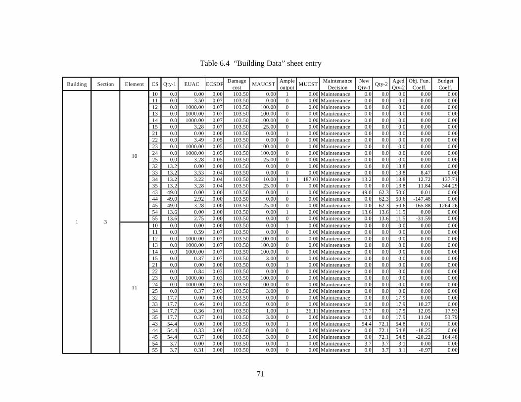
71

Table 6.4 “Building Data” sheet entry

Building Section Element CS Qty-1 EUAC ECSDF Damage cost MAUCST Ample

output MUCST Maintenance Decision

New Qty-1 Qty-2 Aged

Qty-2Obj. Fun.

Coeff.Budget Coeff.

10 0.0 0.00 0.00 103.50 0.00 1 0.00 Maintenance 0.0 0.0 0.0 0.00 0.0011 0.0 3.50 0.07 103.50 0.00 0 0.00 Maintenance 0.0 0.0 0.0 0.00 0.0012 0.0 1000.00 0.07 103.50 100.00 0 0.00 Maintenance 0.0 0.0 0.0 0.00 0.0013 0.0 1000.00 0.07 103.50 100.00 0 0.00 Maintenance 0.0 0.0 0.0 0.00 0.0014 0.0 1000.00 0.07 103.50 100.00 0 0.00 Maintenance 0.0 0.0 0.0 0.00 0.0015 0.0 3.28 0.07 103.50 25.00 0 0.00 Maintenance 0.0 0.0 0.0 0.00 0.0021 0.0 0.00 0.00 103.50 0.00 1 0.00 Maintenance 0.0 0.0 0.0 0.00 0.0022 0.0 3.49 0.05 103.50 0.00 0 0.00 Maintenance 0.0 0.0 0.0 0.00 0.0023 0.0 1000.00 0.05 103.50 100.00 0 0.00 Maintenance 0.0 0.0 0.0 0.00 0.0024 0.0 1000.00 0.05 103.50 100.00 0 0.00 Maintenance 0.0 0.0 0.0 0.00 0.0025 0.0 3.28 0.05 103.50 25.00 0 0.00 Maintenance 0.0 0.0 0.0 0.00 0.0032 13.2 0.00 0.00 103.50 0.00 0 0.00 Maintenance 0.0 0.0 13.8 0.00 0.0033 13.2 3.53 0.04 103.50 0.00 0 0.00 Maintenance 0.0 0.0 13.8 8.47 0.0034 13.2 3.22 0.04 103.50 10.00 1 187.03 Maintenance 13.2 0.0 13.8 12.72 137.7135 13.2 3.28 0.04 103.50 25.00 0 0.00 Maintenance 0.0 0.0 13.8 11.84 344.2943 49.0 0.00 0.00 103.50 0.00 1 0.00 Maintenance 49.0 62.3 50.6 0.01 0.0044 49.0 2.92 0.00 103.50 0.00 0 0.00 Maintenance 0.0 62.3 50.6 -147.48 0.0045 49.0 3.28 0.00 103.50 25.00 0 0.00 Maintenance 0.0 62.3 50.6 -165.88 1264.2654 13.6 0.00 0.00 103.50 0.00 1 0.00 Maintenance 13.6 13.6 11.5 0.00 0.0055 13.6 2.75 0.00 103.50 0.00 0 0.00 Maintenance 0.0 13.6 11.5 -31.59 0.0010 0.0 0.00 0.00 103.50 0.00 1 0.00 Maintenance 0.0 0.0 0.0 0.00 0.0011 0.0 0.59 0.07 103.50 0.00 0 0.00 Maintenance 0.0 0.0 0.0 0.00 0.0012 0.0 1000.00 0.07 103.50 100.00 0 0.00 Maintenance 0.0 0.0 0.0 0.00 0.0013 0.0 1000.00 0.07 103.50 100.00 0 0.00 Maintenance 0.0 0.0 0.0 0.00 0.0014 0.0 1000.00 0.07 103.50 100.00 0 0.00 Maintenance 0.0 0.0 0.0 0.00 0.0015 0.0 0.37 0.07 103.50 3.00 0 0.00 Maintenance 0.0 0.0 0.0 0.00 0.0021 0.0 0.00 0.00 103.50 0.00 1 0.00 Maintenance 0.0 0.0 0.0 0.00 0.0022 0.0 0.84 0.03 103.50 0.00 0 0.00 Maintenance 0.0 0.0 0.0 0.00 0.0023 0.0 1000.00 0.03 103.50 100.00 0 0.00 Maintenance 0.0 0.0 0.0 0.00 0.0024 0.0 1000.00 0.03 103.50 100.00 0 0.00 Maintenance 0.0 0.0 0.0 0.00 0.0025 0.0 0.37 0.03 103.50 3.00 0 0.00 Maintenance 0.0 0.0 0.0 0.00 0.0032 17.7 0.00 0.00 103.50 0.00 0 0.00 Maintenance 0.0 0.0 17.9 0.00 0.0033 17.7 0.46 0.01 103.50 0.00 0 0.00 Maintenance 0.0 0.0 17.9 10.27 0.0034 17.7 0.36 0.01 103.50 1.00 1 36.11 Maintenance 17.7 0.0 17.9 12.05 17.9335 17.7 0.37 0.01 103.50 3.00 0 0.00 Maintenance 0.0 0.0 17.9 11.94 53.7943 54.4 0.00 0.00 103.50 0.00 1 0.00 Maintenance 54.4 72.1 54.8 0.01 0.0044 54.4 0.33 0.00 103.50 0.00 0 0.00 Maintenance 0.0 72.1 54.8 -18.25 0.0045 54.4 0.37 0.00 103.50 3.00 0 0.00 Maintenance 0.0 72.1 54.8 -20.22 164.4854 3.7 0.00 0.00 103.50 0.00 1 0.00 Maintenance 3.7 3.7 3.1 0.00 0.0055 3.7 0.31 0.00 103.50 0.00 0 0.00 Maintenance 0.0 3.7 3.1 -0.97 0.00

10

11

1 3

72

Table 6.5 Column content description for the “Building Data” sheet

Column Number Column Content Description

1 Building number 2 Section number 3 Element number 4 Element initial condition state and suggested final condition state 5 Quantity of element at initial condition state

6 Equivalent, uniform annual cost for improving the element from the initial condition state to the final condition state

7 Element Condition State Damage factor at initial condition state 8 Damage cost

9 Maintenance action unit cost of maintaining, improving or replacing an element

10 Ampl output, the optimum value of the decision variables obtained from AMPL

11 Maintenance and user cost resulting from implementing the selected maintenance action

12 Maintenance or Re-roof decision when MUCST is compared to the equivalent uniform annual re-roof cost

13 Element quantity available at each condition state based on the maintenance or re-roof decision

14 Addition of all element quantity improved to or remained at each condition state

15 Element quantities aged using Markov Chain. The aged quantities will serve as element initial quantities for next year analysis

16 Objective function coefficient, calculated as: Aged Qty_2 * (ECSDF * Damage cost – EUAC)

17 Budget constraint coefficient, calculated as: Aged Qty_2 * MAUCST

6.3 AMPL Operations

AMPL is the acronym for A Mathematical Programming Language. AMPL is a

comprehensive, powerful and flexible algebraic modeling language for the linear, nonlinear

and integer programming problems often encountered in optimization. It uses familiar

algebraic notation to express models concisely, while allowing the separation of model from

the data file. This feature helps in modifying and maintaining the model by allowing sets,

73

variables and constraints to be added, changed or deleted. The separation feature helps also

in updating the data file quickly. AMPL is the software program used in the research to

perform the optimization task. AMPL uses the branch and bound algorithm and CPLEX for

its solver.

The model files required by AMPL are generated using Excel. A visual basic

program, VB, generates the model file required for the first year analysis, while the visual

basic program VB1 generates the maintenance model file required for the remaining years of

the analysis horizon. VB3 is a third visual basic program used to generate the re-roofing

model file required for all years in the analysis horizon when using the separated budget

approach.

The data file, containing the parameter values required to run the optimization model,

is created in advance and stored in a path retrievable by AMPL. There are two data files. The

first data file, “data.dat”, contains the data required to run the maintenance model generated

by both VB and VB1. The second data file, “r_data.dat”, is used to run the re-roofing model

generated by VB3. Both data files can be found in Appendix B3.

The following commands are used with AMPL to obtain the optimal value of the

decision variables for each year in the analysis horizon for the maintenance part of the

analysis when performing the separated budget approach analysis (i represents the analyzed

year):

ampl: Reset; ampl: model”/afs/unity.ncsu.edu/users/a/aaalibra/outputs/model_year i.mod”; ampl: data”afs/unity.ncsu.edu/users/a/aaalibra/data.dat”; ampl: solve; ampl: print {i in I1, j in J1, l in L1, k in K1} x [i, j, l, k]>output; ampl: close output;

The following commands are fed into AMPL to obtain the optimal value of the decision

74

variables for each year in the analysis horizon. These commands are only used for the re-

roofing part of the analysis when performing the separated budget analysis approach (i

represents the analysis year):

ampl: Reset; ampl: model”/afs/unity.ncsu.edu/users/a/aaalibra/outputs/reroof_year i.mod”; ampl: data”afs/unity.ncsu.edu/users/a/aaalibra/r_data.dat”; ampl: solve; ampl: print {n in N1} x [n]>output; ampl: close output;

6.4 Separated Budget Optimization

This optimization is called “separated budget” because two budgets are used in

performing separate optimizations. The first budget, $54,000, is used to optimize

maintenance work. Maintenance work includes repairing or replacement of roof elements

only. With this budget no re-roofing is performed. The second budget is the capital budget,

$246,000, and is used to perform re-roofing work. Re-roofing includes replacing all

elements of a roof section. The steps followed to perform the analysis are shown in Figure

6.1.

75

Figure 6.1 Flowchart for use of Excel and Ampl to optimize roof maintenance using the separated budget approach

76

Figure 6.1 Continued

77

6.4.1 First Year Analysis

The input data are entered in “Initial Quantity” sheet. The data is then displayed in

column 5 of “Initial Building Data” sheet as explained earlier in the chapter. Before starting

the optimization, the initial element quantities displayed in column 5 in “Initial Building

Data” sheet are copied from and pasted in column 5 of “Building Data” sheet. The Visual

Basic program VB is then run from the “Initial Building Data” sheet (see figure 6.1). A

dialog box will appear asking the user to enter the maintenance budget for the analysis. By

entering the budget a binary integer linear program text file is created in an algebraic

modeling language readable by AMPL. The output file generated by VB is named

“model_year1.mod” and is stored in a path retrievable by AMPL. The VB code used to

generate “model_year1.mod” text file can be found in Appendix B1.1. A sample generated

“model_year1.mod” file can be found in Appendix B2.1.

After obtaining the output file resulting from performing the optimization using

AMPL, a second Visual Basic program, VB2, is run from the “Building Data” sheet. VB2

reads the output file generated by AMPL containing the optimized values of the decision

variables. By executing VB2, a message box appears notifying the user that a file called

“ampl_output.cvs” is created. The created file is an Excel file containing the optimized

values of the maintenance decision variables generated by AMPL but translated by Excel

from binary format to ascii or text format. The binary decision variables will be displayed

column wise. The contents of “ampl_output.cvs” are then copied and pasted in column 10 of

“Building Data” sheet. The VB2 code used for this step can be found in Appendix B1.3.

A third Visual Basic program, VB3, will be run from the “Decision” sheet. A dialog

box appears asking the user to enter the budget available for re-roofing. By entering the

78

budget, a file named “reroof_year.mod” is created in an algebraic modeling language

readable by AMPL, and stored in a path retrievable by AMPL. The VB3 code used to

generate “reroof_year.mod can be found in Appendix B1.4. An example of the file

“reroof_year.mod” generated by VB3 can be found in Appendix B2.2.

After obtaining the optimization results from AMPL, a forth Visual Basic program,

VB4, is run. VB4 reads the output file generated by AMPL containing the optimized values

of the re-roofing decision variables. By executing VB4, a message box appears notifying the

user that a file called “ampl_r_output.cvs” is created. The created file is an Excel file

containing the optimized values of the re-roofing decision variables generated by AMPL but

translated by Excel from binary format to ascii or text format. The binary decision variables

are displayed column wise. The values of the later file are copied and pasted into the “Ampl

Output” column in the “Decision” sheet. The VB4 code used for this step can be found in

Appendix B1.5. At this point, the analysis for the first year is completed.

6.4.2 Remaining Years Analysis

Before starting the analysis of the next year, the aged element quantities in column 15

of “Building data” sheet are copied and pasted in column 5 of the same sheet. To start the

next year analysis, VB1 (see Figure 6.1) is run. A dialog box appears asking the user to enter

the maintenance budget for the analysis. By entering the budget a message box will appear

telling the user that a file called “model_yaer.mod” is created. The created file is in an

algebraic modeling language readable by AMPL and will be stored in a path retrievable by

AMPL. The VB1 code used to generate the binary linear program text file can be found in

Appendix B1.2. An example of the file “model_year.mod” generated by VB1 can be found

79

in Appendix B2.1. After obtaining the output file resulting from performing the optimization

using AMPL, VB2 is run from “Building Data” sheet and the decision variable values in

“ampl_output.cvs” are copied into column 10 as explained in the first year analysis. VB3

and VB4 will also be run from “Decision” sheet as explained in the previous section.

The steps in this section are repeated for the number of years remaining in the

analysis horizon. The steps followed to perform the analysis for the separated budget

approach are shown in Figure 6.1.

6.5 Combined Budget Optimization

This step is used to assess the total budget available to the DM&R. The hypothesis is

that a combined budget will show better future savings when compared to the analysis

approach results of the separated budgets discussed earlier.

In the combined budget approach, both the available budget for maintenance and the

available budget for re-roofing are combined and considered to be the total budget used to

optimize roof maintenance.

The Excel file used in the previous approach is also be used for this approach. All

sheets are used except for the “Decision” sheet. Since the maintenance and re-roofing

budgets are combined into one budget, this approach will perform only the first optimization

of the previous approach. For this reason VB3 and VB4 will not be used and AMPL will

only be used to run the first optimization of the separated budget approach using the same

commands.

The steps followed to perform one budget analysis for the combined budget approach

are similar to the steps followed to perform one budget analysis for the separated budget

80

analysis except for the re-roofing part of the analysis that will not be executed. The steps

followed to perform one year analysis of the combined budgets are explained below and

shown in Figure 6.2.

6.5.1 First Year Analysis

The input data are entered in “Initial Quantity” sheet. The data is then displayed in

column 5 of “Initial Building Data” sheet as explained earlier in the chapter. Before starting

the optimization, the initial element quantities displayed in column 5 in “Initial Building

Data” sheet are copied from and pasted in column 5 of “Building Data” sheet. A Visual

Basic program called VB is then run from “Initial Building Data” sheet (see Figure 6.2). A

dialog box will appear asking the user to enter the maintenance budget for the analysis. By

entering the budget, a binary integer linear program text file is created in an algebraic

modeling language readable by AMPL. The output file generated by VB will be called

“model_year1.mod” and will be stored in path retrievable by AMPL. The VB code used to

generate “model_year1.mod” text file can be found in Appendix B1.1. A sample generated

“model_year1.mod” file can be found in Appendix B2.1.

After obtaining the output file resulting from performing the optimization using

AMPL, a second Visual Basic program, VB2, is run from “Building Data” sheet. VB2 will

read the output file generated by AMPL containing the optimized values of the decision

variables. By executing VB2, a message box will appear notifying the user that a file called

“ampl_output.cvs” is created. The created file is an Excel file containing the optimized

values of the maintenance decision variables generated by AMPL but translated by Excel

from binary format to ascii or text format. The binary decision variables will be displayed

81

column wise. The content of “ampl_output.cvs” are then copied and pasted in column 10 of

“Building Data” sheet. The VB2 code used for this step can be found in Appendix B1.3.

Upon reaching this step, the analysis of the first year is completed.

6.5.2 Remaining Years Analysis

Before starting the analysis of the next year, the aged element quantities in column 15

of “Building data” sheet are copied and pasted in column 5 of the same sheet. To start the

next year analysis, VB1 (see Figure 6.2), is run. A dialog box will appear asking the user to

enter the maintenance budget for the analysis. By entering the budget a message box will

appear telling the user that a file called “model_year.mod” is created. The created file is in

an algebraic modeling language readable by AMPL and will be stored in a path retrievable

by AMPL. The VB1 code used to generate the binary linear program text file can be found

in Appendix B1.2. An example of the file “model_year.mod” generated by VB1 can be

found in Appendix B2.1. After obtaining the outputs file resulting from performing the

optimization using AMPL, VB2 is run from “Building Data” sheet and the decision variable

values in “ampl_output.cvs” are copied into column 10 as explained in the first year analysis.

The steps in this section are repeated for the number of years remaining in the

analysis horizon. The steps followed to perform the analysis for the combined budget

approach are shown in Figure 6.2.

82

Figure 6.2 Flowchart for use of Excel and AMPL to optimize roof maintenance using

combined budget approach

83

Figure 6.2 Continued

84

7. ANALYSIS AND RESULTS

This chapter presents an evaluation of the impact of different budget levels and real

rates of return on the model outputs. The results from the analysis are the user costs, total

costs and the weighted average condition state of each roof element. The user costs and total

costs will be used as indicators of cost effects the DM&R may encounter using the Decision

Support System. Better maintenance of roofs results in a higher condition state of the roof

elements and a reduction in the user costs. However, better maintenance results in increases

in maintenance costs offsetting some of the user cost savings.

The analyses conducted are divided into three groups to evaluate the optimization

model. The first group examines the effect of using a combined budget approach vs. a

separated budget approach. The second group examines the sensitivity of the model to

budget reductions and increases. The last group examines the sensitivity of the model to

variations in the required real rates of return. The three groups are shown in Table 7.1.

7.1 Separated Vs. Combined Budgets

As mentioned in the previous chapter, the DM&R has two budgets: the maintenance

budget, which is available for all maintenance work including replacement of individual

roof elements, and the capital budget, available to the department for re-roofing purposes.

This section will present the optimization results from using the two budgets separately,

$54,000 for maintenance work and $246,000 for re-roofing work, versus combining the two

85

budgets and considering it to be the only budget available and used for maintenance work or

re-roofing.

Table 7.1 Analysis groups

Total budget Real Rate of ReturnSeparated $54,000 maintenance + $246,000 re-roofing 3.0%Combined $300,000 3.0%Budget 1 $200,000 3.0%Budget 2 $250,000 3.0%Budget 3 $300,000 3.0%Budget 4 $350,000 3.0%Budget 5 $400,000 3.0%RRR 1 $300,000 1.5%RRR 2 $300,000 3.0%RRR 3 $300,000 4.5%RRR 4 $300,000 6.0%RRR 5 $300,000 7.5%

Group

3

2

1

The User costs resulting from the separated budget maintenance optimization and

combined budget optimization are shown in Table 7.2 and Figure 7.1.

Table 7.2 User costs for the separated and combined budget cases

Difference ($)54K & 246K 300K 54K-300K

1 130,912 109,069 21,842 2 282,068 185,676 96,392 3 438,096 271,675 166,421 4 518,957 334,341 184,616 5 558,334 368,194 190,139 6 559,835 376,320 183,515 7 552,484 356,988 195,495 8 540,056 314,721 225,335 9 523,633 263,808 259,825 10 488,968 205,652 283,315 11 445,650 138,441 307,209 12 399,281 79,230 320,051 13 349,705 33,644 316,061 14 301,206 19,001 282,205 15 270,692 6,600 264,092

Sum 6,359,877 3,063,362 3,296,515

Year User Cost ($)

86

-

100,000

200,000

300,000

400,000

500,000

600,000

0 1 2 3 4 5 6 7 8 9 10 11 12 13 14 15 16

Year

Use

r cos

t ($)

300K

54K & 246K

Figure 7.1 User costs for the separated and combined budget cases

From the results of this analysis, the user costs of the combined budget are always

lower than the user costs when the budget is separated. Table 7.2 and Figure 7.2 show the

difference between the resulting user costs for the two budget approaches. It is also shown

that the difference between the two user costs reaches a peak of about $320,000.

The results of this analysis indicate that it is better to utilize the total combined

budget available to perform maintenance and re-roofing rather than constrain the budget in

fixed categories. Based on these results, the combined budget approach will be used when

investigating the sensitivity of user costs and weighted average condition state to different

budget levels and real rates of return.

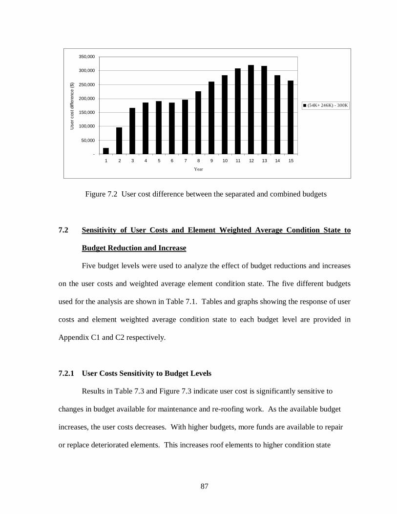
87

-

50,000

100,000

150,000

200,000

250,000

300,000

350,000

1 2 3 4 5 6 7 8 9 10 11 12 13 14 15

Year

Use

r cos

t diff

eren

ce ($

)

(54K+ 246K) - 300K

Figure 7.2 User cost difference between the separated and combined budgets

7.2 Sensitivity of User Costs and Element Weighted Average Condition State to

Budget Reduction and Increase

Five budget levels were used to analyze the effect of budget reductions and increases

on the user costs and weighted average element condition state. The five different budgets

used for the analysis are shown in Table 7.1. Tables and graphs showing the response of user

costs and element weighted average condition state to each budget level are provided in

Appendix C1 and C2 respectively.

7.2.1 User Costs Sensitivity to Budget Levels

Results in Table 7.3 and Figure 7.3 indicate user cost is significantly sensitive to

changes in budget available for maintenance and re-roofing work. As the available budget

increases, the user costs decreases. With higher budgets, more funds are available to repair

or replace deteriorated elements. This increases roof elements to higher condition state

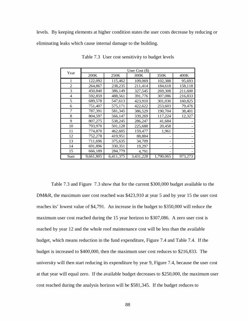
88

levels. By keeping elements at higher condition states the user costs decrease by reducing or

eliminating leaks which cause internal damage to the building.

Table 7.3 User cost sensitivity to budget levels

200K 250K 300K 350K 400K1 122,092 115,462 109,069 102,388 95,693 2 264,867 238,235 211,414 184,618 158,118 3 450,840 386,149 327,545 269,308 211,600 4 592,859 488,561 391,776 307,086 216,833 5 689,578 547,613 423,910 301,030 160,825 6 751,407 575,171 422,622 253,603 79,476 7 787,391 581,345 386,529 190,704 38,401 8 804,597 566,147 339,269 117,224 12,327 9 807,275 538,245 286,247 41,684 - 10 793,970 501,128 225,688 20,458 - 11 774,870 462,605 159,477 1,961 - 12 752,278 419,951 88,884 - - 13 711,696 375,635 34,709 - - 14 691,896 330,351 19,297 - - 15 666,189 284,779 4,791 - -

Sum 9,661,805 6,411,375 3,431,228 1,790,065 973,273

Year User Cost ($)

Table 7.3 and Figure 7.3 show that for the current $300,000 budget available to the

DM&R, the maximum user cost reached was $423,910 at year 5 and by year 15 the user cost

reaches its’ lowest value of $4,791. An increase in the budget to $350,000 will reduce the

maximum user cost reached during the 15 year horizon to $307,086. A zero user cost is

reached by year 12 and the whole roof maintenance cost will be less than the available

budget, which means reduction in the fund expenditure, Figure 7.4 and Table 7.4. If the

budget is increased to $400,000, then the maximum user cost reduces to $216,833. The

university will then start reducing its expenditure by year 9, Figure 7.4, because the user cost

at that year will equal zero. If the available budget decreases to $250,000, the maximum user

cost reached during the analysis horizon will be $581,345. If the budget reduces to

89

$200,000, then the maximum user cost will increase to $807,275. In both the $250,000 and

$200,000 budget, the fund expenditure will remain constant and equal to the available

budget, Figure 7.4.

-

100,000

200,000

300,000

400,000

500,000

600,000

700,000

800,000

900,000

0 1 2 3 4 5 6 7 8 9 10 11 12 13 14 15 16

Year

Use

r cos

t ($)

400K

350K

300K

250K

200K

Figure 7.3 User cost sensitivity to budget levels

The total cost to the university is the sum of the actual budget used plus the user cost

resulting from deteriorated roof elements. Figure 7.5 and Table 7.5 show that the total cost

decreases with the increase of the budget for element maintenance and replacement. It also

shows that before year 3, the higher the budget, the higher the total cost. This changes to the

opposite beyond year three and continues throughout the analysis horizon. Figure 7.5 and

Table 7.5 show that the lowest budget needed to maintain roof elements at an acceptable

levels (CS 4 and 5) is around $200,000. This is only true after bringing all deteriorated

90

elements to condition state 4 or 5 by maintenance or replacement with higher initial budget

levels.

Figure 7.4 and Table 7.4 show the actual fund expenditure for different budget levels.

In the long run, the higher the budget available, the lower the total cost to university even if

the total funds expended increase initially with the increase of available budget.

0

50,000

100,000

150,000

200,000

250,000

300,000

350,000

400,000

450,000

0 1 2 3 4 5 6 7 8 9 10 11 12 13 14 15 16

Year

Fund

exp

endi

ture

($) 200K

250K

300K

350K

400K

Figure 7.4 Funds expended for different budget levels

91

Table 7.4 Funds expended for different budget levels

200K 250K 300K 350K 400K1 199,498 249,828 299,945 349,777 399,9152 199,954 249,983 299,993 349,956 399,9533 199,997 249,961 299,997 349,997 400,0004 199,998 249,974 299,968 349,998 399,9955 199,993 249,999 299,989 349,999 399,9896 199,988 249,999 299,998 349,999 399,9947 199,998 249,994 299,989 349,993 399,9918 199,999 249,996 299,998 349,996 399,9979 199,999 249,998 299,996 349,988 324,06110 199,999 249,997 299,999 349,996 203,13911 199,999 249,998 299,996 349,518 205,07912 199,999 250,000 299,999 223,308 206,65513 200,000 250,000 299,986 200,215 207,93414 200,000 249,993 299,970 203,093 208,97115 200,000 250,000 299,980 205,331 209,813

Sum 2,999,421 3,749,720 4,499,805 4,681,164 4,765,485

Budget Used ($)Year

0

100,000

200,000

300,000

400,000

500,000

600,000

700,000

800,000

900,000

1,000,000

1,100,000

0 1 2 3 4 5 6 7 8 9 10 11 12 13 14 15 16

Year

Tota

l cos

t ($)

200K

250K

300K

350K

400K

Figure 7.5 Total cost for different budget levels

92

Table 7.5 Total cost for different budget levels

200K 250K 300K 350K 400K1 321,590 365,290 409,014 452,165 495,6082 464,821 488,218 511,407 534,575 558,0713 650,837 636,110 627,542 619,305 611,6004 792,857 738,534 691,744 657,085 616,8285 889,571 797,613 723,899 651,029 560,8146 951,394 825,169 722,620 603,601 479,4717 987,389 831,338 686,518 540,696 438,3918 1,004,596 816,143 639,267 467,220 412,3249 1,007,275 788,244 586,243 391,672 324,06110 993,969 751,125 525,688 370,455 203,13911 974,869 712,603 459,474 351,479 205,07912 952,277 669,951 388,883 223,308 206,65513 911,696 625,635 334,695 200,215 207,93414 891,896 580,344 319,268 203,093 208,97115 866,189 534,779 304,771 205,331 209,813

Sum 12,661,226 10,161,095 7,931,033 6,471,229 5,738,757

Total Cost ($)Year

7.2.2 Element Weighted Average Condition State Sensitivity to Budget Levels

From Tables and Figures in Appendix C2 showing the sensitivity of each roof

element weighted average condition state to budget changes, it is found that only three roof

elements are significantly sensitive to budget changes. Figures 7.6, 7.7 and 7.8 show the

sensitivity of single-ply membrane, multiple-ply membrane and shingles respectively to

budget changes.

Figure 7.6 shows that the lower the budget the later the single-ply membrane element

reaches a higher condition state. It is shown from the sensitivity analysis also that the

element reaches condition state 4 from the first analysis year except for budgets of $200,000

and $250,000 where the element reaches condition state 4 at year 8 and 3 respectively.

93

Figure 7.6 and Table 7.6 show that the single-ply membrane has a relatively low sensitivity

to changes in budget levels since the changes in its condition state ranges between 3.82 and

4.74.

0

1

2

3

4

5

0 1 2 3 4 5 6 7 8 9 10 11 12 13 14 15 16

Year

Con

ditio

n st

ate

wei

ghte

d av

erag

e

200K250K300K350K400K

Figure 7.6 Single-ply membrane condition sensitivity to budget level

Table 7.6 Single-ply membrane condition sensitivity to budget level

200K 250K 300K 350K 400K

0 3.82 3.82 3.82 3.82 3.821 3.93 3.98 4.04 4.09 4.142 3.93 3.96 3.99 4.02 4.053 3.94 4.02 4.03 4.04 4.064 3.94 4.10 4.10 4.11 4.125 3.94 4.18 4.18 4.18 4.196 3.95 4.26 4.26 4.26 4.267 3.98 4.33 4.32 4.32 4.428 4.03 4.38 4.37 4.37 4.649 4.09 4.42 4.41 4.42 4.7110 4.18 4.44 4.44 4.60 4.7111 4.27 4.46 4.46 4.73 4.7112 4.34 4.48 4.46 4.72 4.7113 4.47 4.49 4.50 4.72 4.7114 4.53 4.50 4.63 4.72 4.7115 4.53 4.50 4.74 4.72 4.71

YearSingle-ply membrane condition state weighted average

94

With the current budget available to the DM&R the single-ply membrane element

improves to the highest condition state reached by the element at year 15, as shown in Table

7.6. An increase in the budget to $350,000 allows the element to reach its highest condition

state at year 11. An increase in the budget to $400,000 allows the element to reach its

highest condition state at year 9. Reducing the available budget to $250,000 or $200,000 will

cause the element to reach its highest condition state at a year out side our analysis horizon.

Figure 7.7 shows the sensitivity of the multiple-ply membrane to changes in budget

levels. As the available budget for maintenance decreases the element reaches a higher

condition states at later years when compared to the same element but with a higher

maintenance budget. The multiple-ply membrane has a relatively high sensitivity to budget

changes since its condition state ranges between 1.29 and 4.81, as shown in Figure 7.7 and

Table 7.7.

95

0

1

2

3

4

5

0 1 2 3 4 5 6 7 8 9 10 11 12 13 14 15 16

Year

Con

ditio

n st

ate

wei

ghte

d av

erag

e

200K

250K300K350K400K

Figure 7.7 Multiple-ply membrane condition sensitivity to budget level

Table 7.7 Multiple-ply membrane condition sensitivity to budget level

200K 250K 300K 350K 400K

0 3.23 3.23 3.23 3.23 3.231 3.23 3.23 3.23 3.23 3.232 2.82 2.99 3.16 3.33 3.493 2.30 2.55 2.91 3.26 3.614 1.93 2.22 2.77 3.28 3.815 1.70 2.02 2.72 3.42 4.176 1.56 1.93 2.78 3.68 4.607 1.47 1.92 2.97 4.01 4.748 1.41 2.00 3.21 4.38 4.729 1.36 2.15 3.48 4.75 4.8110 1.33 2.33 3.79 4.73 4.8011 1.30 2.54 4.12 4.77 4.7812 1.31 2.76 4.50 4.80 4.7813 1.29 2.99 4.75 4.78 4.7714 1.31 3.22 4.72 4.77 4.7615 1.45 3.45 4.70 4.77 4.76

Year Multiple-ply membrane condition state weighted average

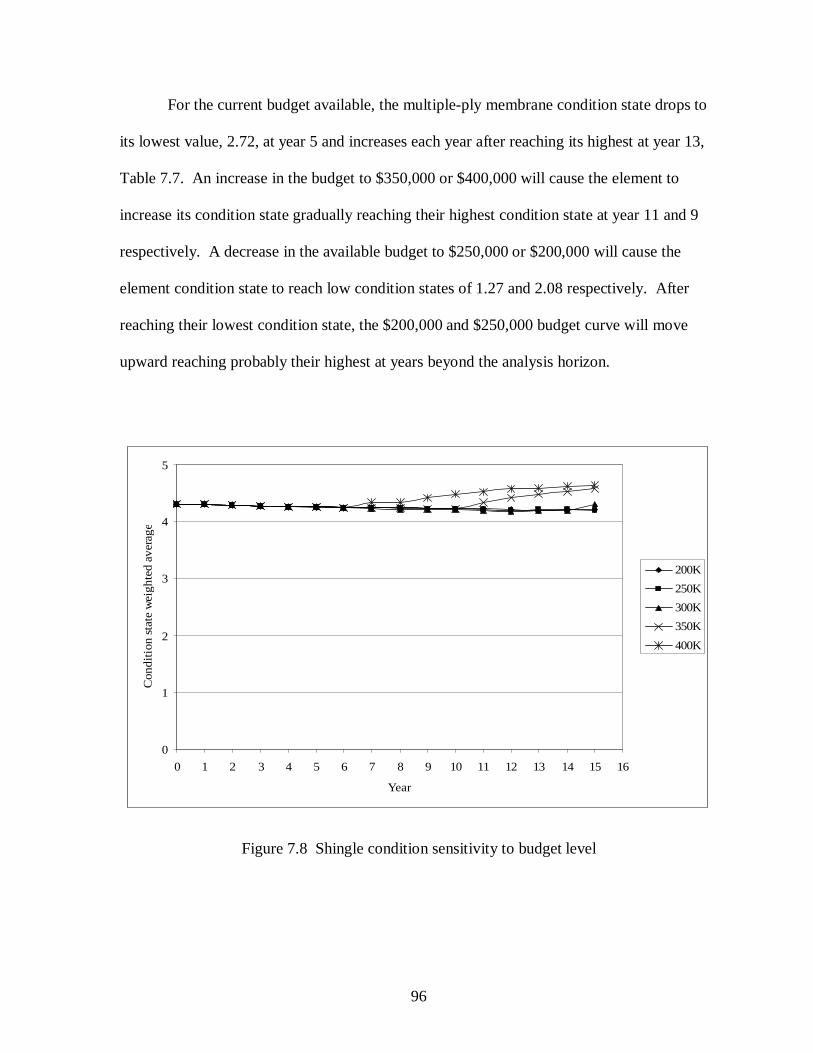
96

For the current budget available, the multiple-ply membrane condition state drops to

its lowest value, 2.72, at year 5 and increases each year after reaching its highest at year 13,

Table 7.7. An increase in the budget to $350,000 or $400,000 will cause the element to

increase its condition state gradually reaching their highest condition state at year 11 and 9

respectively. A decrease in the available budget to $250,000 or $200,000 will cause the

element condition state to reach low condition states of 1.27 and 2.08 respectively. After

reaching their lowest condition state, the $200,000 and $250,000 budget curve will move

upward reaching probably their highest at years beyond the analysis horizon.

0

1

2

3

4

5

0 1 2 3 4 5 6 7 8 9 10 11 12 13 14 15 16

Year

Con

ditio

n st

ate

wei

ghte

d av

erag

e

200K250K300K350K400K

Figure 7.8 Shingle condition sensitivity to budget level

97

Table 7.8 Shingle condition sensitivity to budget level

200K 250K 300K 350K 400K

0 4.31 4.31 4.31 4.31 4.311 4.31 4.31 4.31 4.31 4.312 4.29 4.29 4.29 4.29 4.293 4.27 4.27 4.27 4.27 4.274 4.25 4.26 4.26 4.26 4.265 4.25 4.25 4.25 4.25 4.256 4.24 4.25 4.25 4.25 4.247 4.24 4.24 4.23 4.24 4.348 4.23 4.23 4.21 4.23 4.339 4.23 4.23 4.22 4.23 4.4110 4.23 4.23 4.20 4.23 4.4811 4.22 4.21 4.19 4.33 4.5312 4.21 4.20 4.18 4.41 4.5613 4.20 4.20 4.19 4.48 4.6014 4.20 4.21 4.19 4.53 4.6215 4.21 4.19 4.30 4.57 4.64

Year Shingle condition state weighted average

Figure 7.8 shows the sensitivity of shingles to changes in budget levels. Shingles

show no significant sensitivity to changes in budget level through year 6. Years following

year 6 show a relatively low sensitivity to changes in budget levels where condition states

rage between 4.19 and 4.64.

Table 7.8 shows that for the $300,000 budget the element condition state decreases to

its lowest condition state of 4.18 at year 12 and then the condition state increases reaching

4.30, which is the highest value for this budget at year 15. Increasing the available budget to

$350,000 or $400,000 will cause the element to reach its lowest condition state of 4.23 at

year 8 and 4.24 at year 6 respectively.

98

The highest condition state reached by increasing the available budget to $350,000 is

4.57, while the highest condition state reached by the element due to increasing the budget to

$400,000 is 4.64. A decrease in the available budget to $250,000 will cause a decrease in the

element condition state through the whole analysis horizon reaching its lowest condition state

of 4.19 at year 15. A decrease in the budget to $200,000 will cause a decrease in the element

condition state through the whole analysis horizon. The lowest condition state reached under

the $200,000 budget is 4.20 at years 13 and 14.

7.3 Sensitivity of the User Costs and Element Weighted Average Condition State to

Real Rate of Return

Five Real Rate of Return levels were used to analyze the effect on the user costs and

element weighted average condition state. The five levels used for the analysis are shown in

Table 7.1. Tables and graphs showing the response of user costs and element weighted

average condition state to each Real Rate of Return level are available in Appendix C1 and

C2 respectively.

7.3.1 User Cost Sensitivity to Real Rate of Return Changes

Table 7.9 and Figure 7.9 indicate that user cost is not very sensitivity to changes in

Real Rate of Return levels considered in this analysis. It might be expected that as the Real

Rate of Return increases, the curve of the user cost would move upward. This expectation

would be correct if the Real Rate of Return increase causes the EUAC values to be greater

than the user costs for all elements at all condition states. If this happens the objective

function coefficient would be negative and would not be picked by the model. This would

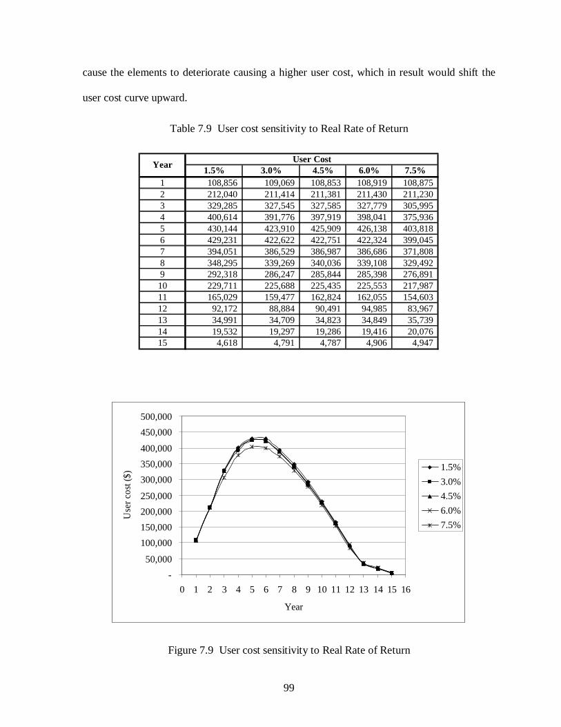
99

cause the elements to deteriorate causing a higher user cost, which in result would shift the

user cost curve upward.

Table 7.9 User cost sensitivity to Real Rate of Return

1.5% 3.0% 4.5% 6.0% 7.5%

1 108,856 109,069 108,853 108,919 108,875 2 212,040 211,414 211,381 211,430 211,230 3 329,285 327,545 327,585 327,779 305,995 4 400,614 391,776 397,919 398,041 375,936 5 430,144 423,910 425,909 426,138 403,818 6 429,231 422,622 422,751 422,324 399,045 7 394,051 386,529 386,987 386,686 371,808 8 348,295 339,269 340,036 339,108 329,492 9 292,318 286,247 285,844 285,398 276,891 10 229,711 225,688 225,435 225,553 217,987 11 165,029 159,477 162,824 162,055 154,603 12 92,172 88,884 90,491 94,985 83,967 13 34,991 34,709 34,823 34,849 35,739 14 19,532 19,297 19,286 19,416 20,076 15 4,618 4,791 4,787 4,906 4,947

Year User Cost

-50,000

100,000150,000200,000250,000

300,000350,000400,000

450,000500,000

0 1 2 3 4 5 6 7 8 9 10 11 12 13 14 15 16

Year

Use

r cos

t ($)

1.5%3.0%4.5%6.0%7.5%

Figure 7.9 User cost sensitivity to Real Rate of Return

100

This was not the case for the Real Rates of Return used in this study. For the

analyzed Real Rates of Return, as the Real Rate of Return increases the EUAC for each roof

element increases too, but the increase never exceeded the user cost. The increase of the

EUAC caused some elements to have an objective function more attractive to be picked by

the optimization model than other elements.

For the 1.5%, 3%, 4.5%, and 6% Real Rates of Return, the increase of the EUAC was

not sufficient to change the model optimized decision. This resulted in having nearly the

same user cost for all four Real Rates of return and their curves are drawn on top of each

other, Figure 7.9, indicating low user cost sensitivity to changes in the Real Rate of Return.

The increase of the EUAC due to the 7.5% Real rate of Return caused the model to

change its optimizing decisions. For this Real Rate of Return, it can be shown from the

analysis results in Appendix C1 that it was more attractive to the model to use more of the

budget to maintain the multiple-ply membrane. Since the single-ply and multiple-ply

membrane are the elements that result in highest user cost if damage occurs to them, any

maintenance or replacement will drop the user costs significantly in comparison to other roof

elements. For this reason the 7.5% resulted in slightly lower total user cost - when compared

to the other analyzed Real Rates of Return - which shifted its user cost curve downward.

7.3.2 Element Weighted Average Condition State Sensitivity to Real Rate of Return

Changes

From Tables and Figures in Appendix C2 showing the sensitivity of each roof

element weighted average condition state to Real Rate of Return changes, it is found that roof

101

element condition state have no significant sensitivity to changes in Real Rates of Return

changes except for multiple-ply membrane, which shows a low sensitivity to Real Rate of

Return changes. Figure 7.10 shows the sensitivity of multiple-ply membrane to changes in

Real Rate of Return.

Table 7.10 and Figure 7.10 show that multiple-ply membrane weighted average

condition state has a very low sensitivity to changes in Real Rates of Return analyzed in this

study except for the 7.5% level. By increasing the Real rate of Return to 7.5% the curve in

Figure 7.10 moves upward. The upward movement of the curve indicates a better element

weighted average condition state compared to the other Real Rate of Return weighted

average. However, this appears to be due to minor switches in actions selected rather than a

general trend.

Table 7.10 Multiple-ply membrane weighted average condition state sensitivity to Real Rate

of Return

1.5% 3.0% 4.5% 6.0% 7.5%0 3.23 3.23 3.23 3.23 3.231 3.23 3.23 3.23 3.23 3.232 3.15 3.16 3.16 3.16 3.163 2.89 2.91 2.91 2.91 2.984 2.72 2.77 2.75 2.75 2.825 2.68 2.72 2.71 2.71 2.786 2.74 2.78 2.78 2.78 2.867 2.92 2.97 2.96 2.97 3.018 3.15 3.21 3.20 3.21 3.249 3.44 3.48 3.48 3.48 3.5110 3.76 3.79 3.78 3.79 3.8111 4.09 4.12 4.10 4.11 4.1312 4.48 4.50 4.49 4.45 4.5613 4.75 4.75 4.75 4.75 4.7514 4.72 4.72 4.72 4.72 4.7215 4.70 4.70 4.70 4.70 4.70

Year Multiple-ply membrane condition state weighted average

102

0

1

2

3

4

5

0 1 2 3 4 5 6 7 8 9 10 11 12 13 14 15 16

Year

Con

ditio

n st

ate

wei

ghte

d av

erag

e

1.5%3.0%4.5%6.0%7.5%

Figure 7.10 Multiple-ply membrane weighted average condition state sensitivity to Real Rate of Return

103

8. CONCLUSIONS AND RECOMMENDATIONS

The main objective of the research was to develop a Decision Support System that

optimizes the allocation of available funds to the DM&R by maximizing the saving in annual

cost through maximizing the total amount of reductions in equivalent uniform annual cost.

Based on the developed methodology and data available or developed for the analysis, this

chapter lists the conclusions of this study and recommendations for future research and

development.

8.1 Conclusions

1. The Decision Support System developed in this study provides an allocation of the

available funds to the Department of Maintenance and Repair that results in optimal sets

of roof element improvement.

2. The combined budget approach produces lower total cost in comparison to the separated

budget approach. This is due to non-optimal restriction of the available budget into fixed

categories in the separated budget approach.

3. For the combined budget approach, the higher the available budget, the lower the

resulting user cost. The analysis shows that the user cost is sensitive to budget levels.

Increasing the funding for roof maintenance and replacement would reduce total costs by

reducing user costs (building damage).

4. For the developed model and data available, the multiple-ply membrane has a high

weighted average condition state sensitivity to budget levels. The single-ply membrane

104

and shingle elements show less condition sensitivity to budget levels in comparison to

multiple-ply membrane. All other elements have shown low condition sensitivity to

budget changes.

5. For the developed model and data available, the user costs show very low sensitivity to

changes in Real Rate of Return.

6. No significant condition sensitivity is shown by any roof elements to changes in Real

Rate of Return except for the multiple-ply membrane where it shows a slight sensitivity.

8.2 Recommendations

1. Expand the study to include the remaining university buildings when the data is available.

To do that, another computer program has to be used due to Excel capacity limitation in

data entry.

2. The values of ECSDF and ACSSL used in this study were estimated with the help of

experts at the Department of Maintenance and Repair. More research would be desirable

to improve the accuracy and precision of this data.

3. Remove the exponential distribution assumption and empirically determine the values of

ACSSL based on historical data to obviate the need to assume any real life distribution,

which is typically extremely difficult to assess.

4. Expand the analysis horizon to test the model adequacy beyond the 15 years.

5. Modify the model developed in this study to incorporate the dependence relationship

between membrane and insulation maintenance and replacement.

6. Allow the element quantity to deteriorate to any condition state in one year in case of

natural disaster or poor element installment.

105

7. The DSS model analysis system needs to be automated so that it becomes user friendly

for optimizing roof maintenance.

106

9. REFERENCES

1. Lee, R. (1976) Building Maintenance Management. Crosby Lockwood Staples, London.

2. Shear, M. (1983) Handbook of Building Maintenance Management. Reston Publishing

Company, Inc. Reston, Virginia. 3. Propeller Head Software, Inc. (2005) Roof Manager. Matthews, NC.

www.roofmanager.com. 4. The Garland Company, Inc. (2005) Garland Roof Asset Management Program.

Cleveland, OH. www.garlandco.com. 5. Bailey D., Brotherson D., Tobiasson W., (1989) Roofer: A Management Tool for

Maintaining Built-Up Roofs. US Army Corps of Engineers and Cold Regions Research & Engineering Laboratory. US Army Corps of Engineers, Construction Engineering Research Laboratory, Champaign, Ill. And National Technical Information Service, Springfield, VA.

6. Shahin M., Bailey D and Brotherson D. (1987) Membrane and Flashing Condition

Indexes for Built-up Roofs. US Army Corps of Engineers, Construction Engineering Research Laboratory, Champaign, Ill., and National Technical Information Service, Springfield, VA.

7. Farid F., Johnston, D., Chen, C., Laverde, M. and Rihani, B. (1988) Feasibility of

Incremental Benefit-Cost Analysis for Optimal Allocation of Limited Budgets to Maintenance, Rehabilitation and Replacement for Bridges, FHWA-DP-71-02, Research Project DTFH71-87-NC-07, Center for Transportation Engineering Studies, Department of Civil Engineering, North Carolina State University, Raleigh, NC, 187 pages.

8. Al-Subhi, K., Johnston, D. and Farid, F. (1989) Optimizing System-Level Bridge

Maintenance, Rehabilitation, and Replacement Decisions. FHWA/NC/89-001, Research Project 88-2, Center for Transportation Engineering Studies, Department of Civil Engineering, North Carolina State University, Raleigh, NC, 274 pages.

9. Jebreen, J. (1995) Bridge Maintenance Level of Service Optimization Based on an

Economic Analysis Approach. A dissertation submitted to the graduate faculty of North Carolina State University in partial fulfillment of the requirements for the degree of Doctoral of Philosophy, Raleigh, NC, 151 pages.

10. Cameron, A. and Ronald S. (1998) Principles and Practices of Heavy Construction.

Prentice Hall, New Jersey.

http://www.roofmanager.com

http://www.garlandco.com

107

11. Paroli, R.M. and Booth, R.J. (1997) Ways to Reduce Blistering Built-Up Roofs. National

Research Council of Canada. ISSN 1206-1220. 12. All American Roofing. (December 2005) www.800roofusa.com. West Los Angeles. 13. Hardy, S. (1998) Time-Saver Details for Roof Design. McGraw-Hill, New York. 14. Bollnow, T. and Crowe J. (2005) Steep-Slope Reroofing Consideration. Professional Roofing.

National Roofing Contractors Association. www.professionalroofing.net. 15. Beall, C. (1999) Thermal and Moisture Protection Manual. McGraw-Hill, New York. 16. R.S Means Company. (1997) Means Building Construction Cost Data. R.S. Means Co.

Kingston, MA.

http://www.800roofusa.com

http://www.professionalroofing.net

108

APPENDIX A

109

APPENDIX A1

This appendix includes the MAUCST matrices of all maintenance elements.


5 0.004

4 5.50 0.003

3 5.50 100.00 0.002

2 5.50 100.00 100.00 0.001

1 5.50 100.00 100.00 100.00 0.00Con

ditio

n st

ate

befo

re m

aint

enan

ce (c

)

Figure A1.1 Single-ply membrane MAUCST ($/SF)


5 0.004

4 7.00 0.003

3 7.00 100.00 0.002

2 7.00 100.00 100.00 0.001

1 7.00 100.00 100.00 100.00 0.00Con

ditio

n st

ate

befo

re m

aint

enan

ce (c

)

Figure A1.2 Multiple-ply membrane MAUCST ($/SF)

110


5 6.004

4 6.00 0.003

3 6.00 1.00 0.002

2 6.00 100.00 100.00 0.001

1 6.00 100.00 100.00 100.00 0.00Con

ditio

n st

ate

befo

re m

aint

enan

ce (c

)

Figure A1.3 Single-ply base flashing MAUCST ($/LF)


5 7.504

4 7.50 0.003

3 7.50 2.00 0.002

2 7.50 100.00 100.00 0.001

1 7.50 100.00 100.00 100.00 0.00Con

ditio

n st

ate

befo

re m

aint

enan

ce (c

)

Figure A1.4 Multiple-ply base flashing MAUCST ($/LF)

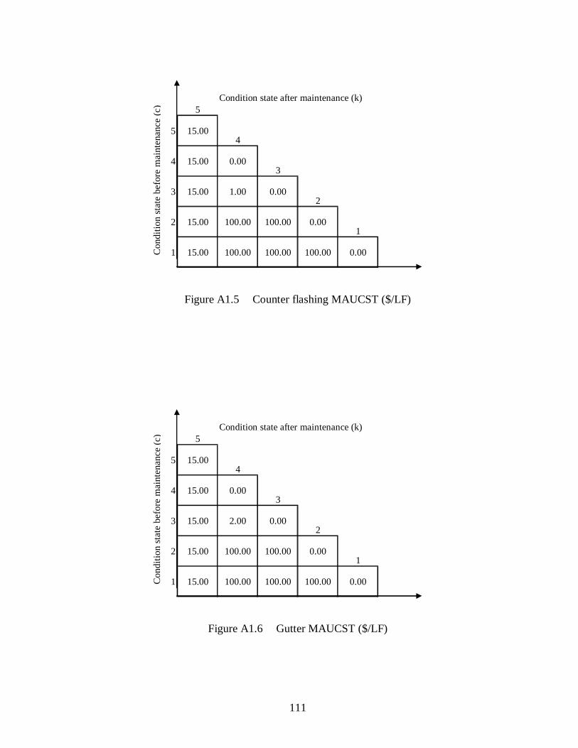
111


5 15.004

4 15.00 0.003

3 15.00 1.00 0.002

2 15.00 100.00 100.00 0.001

1 15.00 100.00 100.00 100.00 0.00Con

ditio

n st

ate

befo

re m

aint

enan

ce (c

)

Figure A1.5 Counter flashing MAUCST ($/LF)


5 15.004

4 15.00 0.003

3 15.00 2.00 0.002

2 15.00 100.00 100.00 0.001

1 15.00 100.00 100.00 100.00 0.00Con

ditio

n st

ate

befo

re m

aint

enan

ce (c

)

Figure A1.6 Gutter MAUCST ($/LF)

112


5 12.004

4 12.00 0.003

3 12.00 4.00 0.002

2 12.00 100.00 100.00 0.001

1 12.00 100.00 100.00 100.00 0.00Con

ditio

n st

ate

befo

re m

aint

enan

ce (c

)

Figure A1.7 Downspout MAUCST ($/LF)


5 35.004

4 35.00 0.003

3 35.00 1.50 0.002

2 35.00 100.00 100.00 0.001

1 35.00 100.00 100.00 100.00 0.00Con

ditio

n st

ate

befo

re m

aint

enan

ce (c

)

Figure A1.8 Drain strainer MAUCST ($/EA)

113


5 25.004

4 25.00 0.003

3 25.00 10.00 0.002

2 25.00 100.00 100.00 0.001

1 25.00 100.00 100.00 100.00 0.00Con

ditio

n st

ate

befo

re m

aint

enan

ce (c

)

Figure A1.9 Coping cap MAUCST ($/EA)


5 3.004

4 3.00 0.003

3 3.00 1.00 0.002

2 3.00 100.00 100.00 0.001

1 3.00 100.00 100.00 100.00 0.00Con

ditio

n st

ate

befo

re m

aint

enan

ce (c

)

Figure A1.10 Termination bar MAUCST ($/LF)

114


5 15.004

4 15.00 0.003

3 15.00 1.00 0.002

2 15.00 100.00 100.00 0.001

1 15.00 100.00 100.00 100.00 0.00Con

ditio

n st

ate

befo

re m

aint

enan

ce (c

)

Figure A1.11 Edge metal MAUCST ($/LF)


5 4.204

4 4.20 0.003

3 4.20 2.00 0.002

2 4.20 100.00 100.00 0.001

1 4.20 100.00 100.00 100.00 0.00Con

ditio

n st

ate

befo

re m

aint

enan

ce (c

)

Figure A1.12 Shingle MAUCST ($/SF)

115


5 30.004

4 30.00 0.003

3 30.00 5.00 0.002

2 30.00 100.00 100.00 0.001

1 30.00 100.00 100.00 100.00 0.00Con

ditio

n st

ate

befo

re m

aint

enan

ce (c

)

Figure A1.13 Slate MAUCST ($/SF)


5 6.004

4 6.00 0.003

3 6.00 1.00 0.002

2 6.00 100.00 100.00 0.001

1 6.00 100.00 100.00 100.00 0.00Con

ditio

n st

ate

befo

re m

aint

enan

ce (c

)

Figure A1.14 Hip/Ridge cap MAUCST ($/LF)

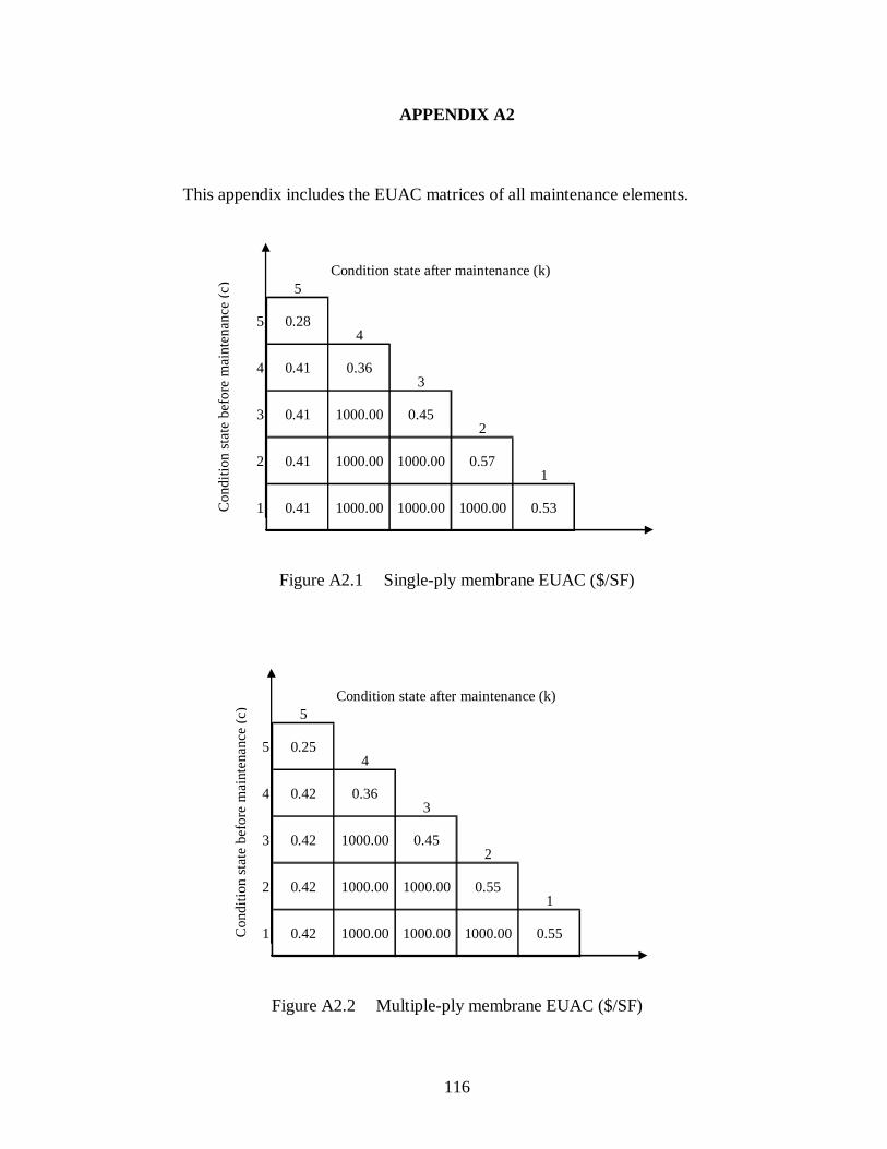
116

APPENDIX A2

This appendix includes the EUAC matrices of all maintenance elements.


5 0.284

4 0.41 0.363

3 0.41 1000.00 0.452

2 0.41 1000.00 1000.00 0.571

1 0.41 1000.00 1000.00 1000.00 0.53Con

ditio

n st

ate

befo

re m

aint

enan

ce (c

)

Figure A2.1 Single-ply membrane EUAC ($/SF)


5 0.254

4 0.42 0.363

3 0.42 1000.00 0.452

2 0.42 1000.00 1000.00 0.551

1 0.42 1000.00 1000.00 1000.00 0.55Con

ditio

n st

ate

befo

re m

aint

enan

ce (c

)

Figure A2.2 Multiple-ply membrane EUAC ($/SF)

117


5 0.344

4 0.48 0.423

3 0.48 0.45 0.732

2 0.48 1000.00 1000.00 0.921

1 0.48 1000.00 1000.00 1000.00 0.89Con

ditio

n st

ate

befo

re m

aint

enan

ce (c

)

Figure A2.3 Single-ply base flashing EUAC ($/LF)


5 0.404

4 0.00 0.483

3 0.57 0.54 0.882

2 0.57 1000.00 1000.00 1.081

1 0.57 1000.00 1000.00 1000.00 0.88Con

ditio

n st

ate

befo

re m

aint

enan

ce (c

)

Figure A2.4 Multiple-ply base flashing EUAC ($/LF)

118


5 1.254

4 1.46 1.303

3 1.46 1.33 1.762

2 1.46 1000.00 1000.00 1.831

1 4.16 1000.00 1000.00 1000.00 1.87Con

ditio

n st

ate

befo

re m

aint

enan

ce (c

)

Figure A2.5 Counter flashing EUAC ($/LF)


5 1.604

4 1.85 1.703

3 1.85 1.76 1.932

2 1.85 1000.00 1000.00 1.931

1 1.85 1000.00 1000.00 1000.00 1.94Con

ditio

n st

ate

befo

re m

aint

enan

ce (c

)

Figure A2.6 Gutter EUAC ($/LF)

119


5 1.554

4 1.79 1.643

3 1.79 1.76 2.442

2 1.79 1000.00 1000.00 2.771

1 1.79 1000.00 1000.00 1000.00 2.56Con

ditio

n st

ate

befo

re m

aint

enan

ce (c

)

Figure A2.7 Downspout EUAC ($/LF)


5 2.854

4 3.38 3.003

3 3.38 3.05 11.672

2 3.38 1000.00 1000.00 12.281

1 3.38 1000.00 1000.00 1000.00 8.05Con

ditio

n st

ate

befo

re m

aint

enan

ce (c

)

Figure A2.8 Drain strainer EUAC ($/EA)

120


5 2.754

4 3.28 2.923

3 3.28 3.22 3.532

2 3.28 1000.00 1000.00 3.491

1 3.28 1000.00 1000.00 1000.00 3.50Con

ditio

n st

ate

befo

re m

aint

enan

ce (c

)

Figure A2.9 Coping cap EUAC ($/EA)


5 0.314

4 0.37 0.333

3 0.37 0.36 0.462

2 0.37 1000.00 1000.00 0.841

1 0.37 1000.00 1000.00 1000.00 0.59Con

ditio

n st

ate

befo

re m

aint

enan

ce (c

)

Figure A2.10 Termination bar EUAC ($/LF)

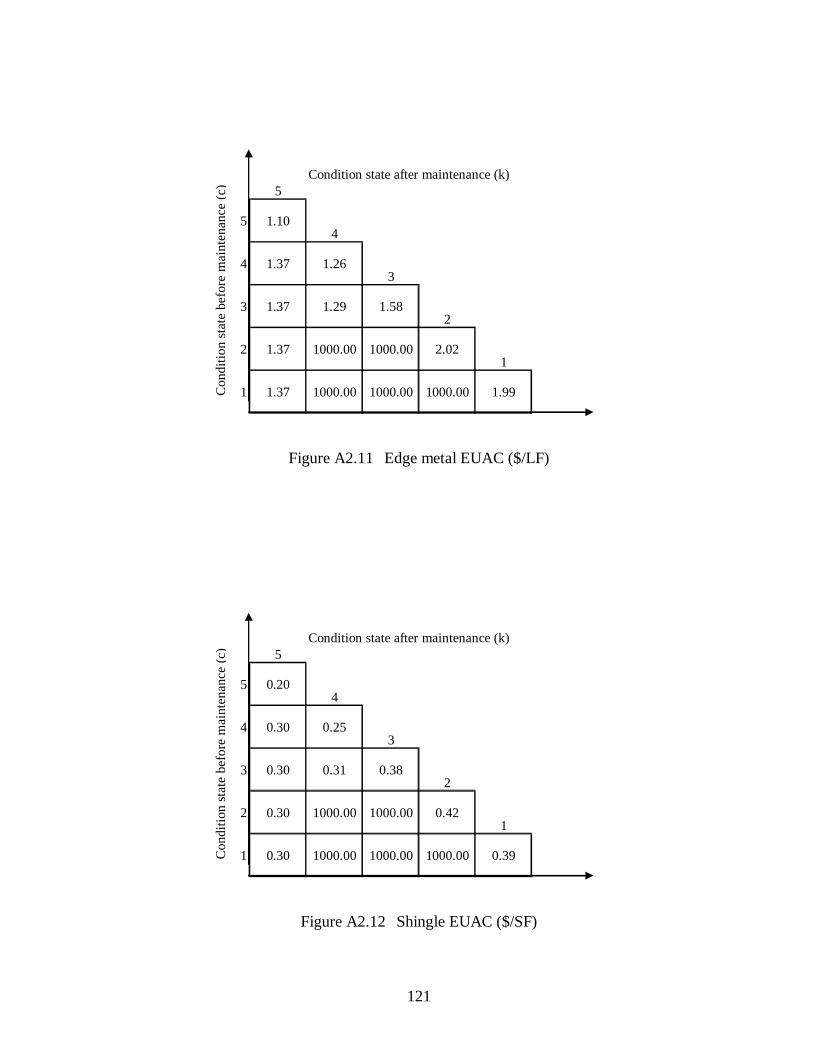
121


5 1.104

4 1.37 1.263

3 1.37 1.29 1.582

2 1.37 1000.00 1000.00 2.021

1 1.37 1000.00 1000.00 1000.00 1.99Con

ditio

n st

ate

befo

re m

aint

enan

ce (c

)

Figure A2.11 Edge metal EUAC ($/LF)


5 0.204

4 0.30 0.253

3 0.30 0.31 0.382

2 0.30 1000.00 1000.00 0.421

1 0.30 1000.00 1000.00 1000.00 0.39Con

ditio

n st

ate

befo

re m

aint

enan

ce (c

)

Figure A2.12 Shingle EUAC ($/SF)

122


5 0.444

4 1.04 0.503

3 1.04 0.65 1.072

2 1.04 1000.00 1000.00 1.191

1 1.04 1000.00 1000.00 1000.00 1.13Con

ditio

n st

ate

befo

re m

aint

enan

ce (c

)

Figure A2.13 Slate EUAC ($/SF)


5 0.264

4 0.39 0.323

3 0.39 0.35 0.482

2 0.39 1000.00 1000.00 0.561

1 0.39 1000.00 1000.00 1000.00 0.48Con

ditio

n st

ate

befo

re m

aint

enan

ce (c

)

Figure A2.14 Hip/Ridge cap EUAC ($/LF)

123

APPENDIX B

124

APPENDIX B1

This appendix includes all the Visual Basic programs used in the analysis:

B1.1 Visual Basic Code (VB)

' Keyboard Shortcut: Ctrl+Shift+I '================================================== ' The file path where the file will be saved in "k:\outputs\" directory '================================================== Sheets("Initial Building Data").Select Open "k:\outputs\model_year_1.mod" For Output As #3 Open "k:\outputs\model_year_1.txt" For Output As #4 '=================================================== ' Writing the header of the model file '=================================================== Print #3, "set I1;" Print #3, "set J1;" Print #3, "set L1;" Print #3, "set K1;" Print #4, "set I1;" Print #4, "set J1;" Print #4, "set L1;" Print #4, "set K1;" msgin: Budget = InputBox("Please enter the Budget: ", "Budget") If Trim(Budget) = "" Then GoTo msgin Print #3, "param budget:= " & Budget & ";" Print #3, " " Print #3, "var x{i in I1,j in J1,l in L1,k in K1}binary;" Print #4, "param budget:= " & Budget & ";" Print #4, " " Print #4, "var x{i in I1,j in J1,l in L1,k in K1}binary;" '=================================================== ' Writing the objective function formula '=================================================== txtmsg = "maximize REUAC:" For i = 2 To 50401 xx = Trim(Cells(i, 10).Value) If Trim(xx) <> "0" And IsNumeric(Trim(xx)) Then

125

a = (((i - 2) \ 3600) + 1) b = (((i - 2) \ 300) + 1) - ((a - 1) * 12) c = (((i - 2) \ 20) + 1) - ((b - 1) * 15) - ((a - 1) * 180) d = Trim(Cells(i, 4).Value) txtmsg = txtmsg & xx & "*x[" & a & "," & b & "," & c & "," & d & "]+" End If Next i For i = 2 To 50401 xx = Trim(Cells(i, 22).Value) If Trim(xx) <> "0" And IsNumeric(Trim(xx)) Then a = (((i - 2 + 50401) \ 3600) + 1) b = (((i - 2 + 50401) \ 300) + 1) - ((a - 1) * 12) c = (((i - 2 + 50401) \ 20) + 1) - ((b - 1) * 15) - ((a - 1) * 180) d = Trim(Cells(i, 16).Value) txtmsg = txtmsg & xx & "*x[" & a & "," & b & "," & c & "," & d & "]+" End If Next i Print #3, Mid(Trim(txtmsg), 1, (Len(Trim(txtmsg))) - 1) & ";" Print #4, Mid(Trim(txtmsg), 1, (Len(Trim(txtmsg))) - 1) & ";" '=================================================== ' Writing the budget constraint formula '=================================================== Print #3, " " Print #3, " " Print #4, " " Print #4, " " txtmsg = "subject to constraint1 :" For i = 2 To 50401 xx = Trim(Cells(i, 11).Value) If Trim(xx) <> "0" And IsNumeric(Trim(xx)) Then a = (((i - 2) \ 3600) + 1) b = (((i - 2) \ 300) + 1) - ((a - 1) * 12) c = (((i - 2) \ 20) + 1) - ((b - 1) * 15) - ((a - 1) * 180) d = Trim(Cells(i, 4).Value) txtmsg = txtmsg & xx & "*x[" & a & "," & b & "," & c & "," & d & "]+" End If Next i For i = 2 To 50401 xx = Trim(Cells(i, 23).Value) If Trim(xx) <> "0" And IsNumeric(Trim(xx)) Then a = (((i - 2 + 50401) \ 3600) + 1) b = (((i - 2 + 50401) \ 300) + 1) - ((a - 1) * 12) c = (((i - 2 + 50401) \ 20) + 1) - ((b - 1) * 15) - ((a - 1) * 180)

126

d = Trim(Cells(i, 16).Value) txtmsg = txtmsg & xx & "*x[" & a & "," & b & "," & c & "," & d & "]+" End If Next i Print #3, Mid(Trim(txtmsg), 1, (Len(Trim(txtmsg))) - 1) & "<=budget;" Print #4, Mid(Trim(txtmsg), 1, (Len(Trim(txtmsg))) - 1) & "<=budget;" '=================================================== ' Writing the bottom of the model file '================================================== Print #3, " " Print #3, " " Print #4, " " Print #4, " " Print#3, "subject to constraint2 {i in I1,j in J1,l in L1}:

x[i,j,l,10]+x[i,j,l,11]+x[i,j,l,12]+x[i,j,l,13]+x[i,j,l,14]+x[i,j,l,15]=1;" Print #3, "subject to constraint3 {i in I1,j in J1,l in L1}:

x[i,j,l,21]+x[i,j,l,22]+x[i,j,l,23]+x[i,j,l,24]+x[i,j,l,25]=1;" Print #3, "subject to constraint4 {i in I1,j in J1,l in L1}:

x[i,j,l,32]+x[i,j,l,33]+x[i,j,l,34]+x[i,j,l,35]=1;" Print #3, "subject to constraint5 {i in I1,j in J1,l in L1}:

x[i,j,l,43]+x[i,j,l,44]+x[i,j,l,45]=1;" Print #3, "subject to constraint6 {i in I1,j in J1,l in L1}:

x[i,j,l,54]+x[i,j,l,55]=1;" Print #4, "subject to constraint2 {i in I1,j in J1,l in L1}:





x[i,j,l,54]+x[i,j,l,55]=1;" '=================================================== ' Closing the file '=================================================== Close #3 Close #4 MsgBox "Creation of the file model is successfully done, The file is saved in K:\outputs\ ", vbInformation, " Done" End Sub

127

B1.2 Visual Basic Code 1 (VB1)

' Keyboard Shortcut: Ctrl+Shift+B '================================================== ' The path where the file will be saved in "K:\outputs\" directory '================================================== Sheets("Building Data").Select Open "K:\outputs\model_year_.mod" For Output As #3 Open "K:\outputs\model_year_.txt" For Output As #4 '=================================================== ' Writing the header of the model file '=================================================== Print #3, "set I1;" Print #3, "set J1;" Print #3, "set L1;" Print #3, "set K1;" Print #4, "set I1;" Print #4, "set J1;" Print #4, "set L1;" Print #4, "set K1;" msgin: Budget = InputBox("Please enter the Budget: ", "Budget") If Trim(Budget) = "" Then GoTo msgin Print #3, "param budget:= " & Budget & ";" Print #3, " " Print #3, "var x{i in I1,j in J1,l in L1,k in K1} binary;" Print #4, "param budget:= " & Budget & ";" Print #4, " " Print #4, "var x{i in I1,j in J1,l in L1,k in K1} binary;" '=================================================== ' Writing the objective function formula '=================================================== txtmsg = "maximize REUAC:" For i = 2 To 50401 xx = Trim(Cells(i, 16).Value) If Trim(xx) <> "0" And IsNumeric(Trim(xx)) Then a = (((i - 2) \ 3600) + 1) b = (((i - 2) \ 300) + 1) - ((a - 1) * 12) c = (((i - 2) \ 20) + 1) - ((b - 1) * 15) - ((a - 1) * 180) d = Trim(Cells(i, 4).Value) txtmsg = txtmsg & xx & "*x[" & a & "," & b & "," & c & "," & d & "]+" End If

128

Next i For i = 2 To 50401 xx = Trim(Cells(i, 35).Value) If Trim(xx) <> "0" And IsNumeric(Trim(xx)) Then a = (((i - 2 + 50401) \ 3600) + 1) b = (((i - 2 + 50401) \ 300) + 1) - ((a - 1) * 12) c = (((i - 2 + 50401) \ 20) + 1) - ((b - 1) * 15) - ((a - 1) * 180) d = Trim(Cells(i, 23).Value) txtmsg = txtmsg & xx & "*x[" & a & "," & b & "," & c & "," & d & "]+" End If Next i Print #3, Mid(Trim(txtmsg), 1, (Len(Trim(txtmsg))) - 1) & ";" Print #4, Mid(Trim(txtmsg), 1, (Len(Trim(txtmsg))) - 1) & ";" '=================================================== ' Writing the budget constraint formula '=================================================== Print #3, " " Print #3, " " Print #4, " " Print #4, " " txtmsg = "subject to constraint1 :" For i = 2 To 50401 xx = Trim(Cells(i, 17).Value) If Trim(xx) <> "0" And IsNumeric(Trim(xx)) Then a = (((i - 2) \ 3600) + 1) b = (((i - 2) \ 300) + 1) - ((a - 1) * 12) c = (((i - 2) \ 20) + 1) - ((b - 1) * 15) - ((a - 1) * 180) d = Trim(Cells(i, 4).Value) txtmsg = txtmsg & xx & "*x[" & a & "," & b & "," & c & "," & d & "]+" End If Next i For i = 2 To 50401 xx = Trim(Cells(i, 36).Value) If Trim(xx) <> "0" And IsNumeric(Trim(xx)) Then a = (((i - 2 + 50401) \ 3600) + 1) b = (((i - 2 + 50401) \ 300) + 1) - ((a - 1) * 12) c = (((i - 2 + 50401) \ 20) + 1) - ((b - 1) * 15) - ((a - 1) * 180) d = Trim(Cells(i, 23).Value) txtmsg = txtmsg & xx & "*x[" & a & "," & b & "," & c & "," & d & "]+" End If Next i Print #3, Mid(Trim(txtmsg), 1, (Len(Trim(txtmsg))) - 1) & "<=budget;"

129

Print #4, Mid(Trim(txtmsg), 1, (Len(Trim(txtmsg))) - 1) & "<=budget;" '=================================================== ' Writing the bottom of the model file '=================================================== Print #3, " " Print #3, " " Print #4, " " Print #4, " " Print #3, "subject to constraint2 {i in I1,j in J1,l in L1}:





x[i,j,l,54]+x[i,j,l,55]=1;" Print #4, "subject to constraint2 {i in I1,j in J1,l in L1}:





x[i,j,l,54]+x[i,j,l,55]=1;" '=================================================== ' Closing the file '=================================================== Close #3 Close #4 MsgBox "Creation of the file model is successfully done, The file is saved in K:\outputs\ ", vbInformation, " Done" End Sub

130

B1.3 Visual Basic Code 2 (VB2) ' Keyboard Shortcut: Ctrl+Shift+R '================================================== ' The file path where the file will be saved in "k:\" ' directory '================================================== Sheets("Building Data").Select Open "K:\output" For Input As #1 '=================================================== ' Read Data character by character from the file and 'store it in jj '=================================================== Do Until EOF(1) Line Input #1, xx For k = 1 To Len(Trim(xx)) DoEvents If Asc(Mid(Trim(xx), k, 1)) = 48 Or Asc(Mid(Trim(xx), k, 1)) = 49 Then jj = jj & Chr(Asc(Mid(Trim(xx), k, 1))) i = i + 1 End If Next k Loop '=================================================== ' Creating CSV file '=================================================== Open "k:\ampl_output_1.csv" For Output As #2 For i = 1 To 50400 DoEvents Print #2, Mid(Trim(jj), i, 1) & "," & Mid(Trim(jj), i + 50400, 1) Next i Close #2 '=================================================== ' Close file and display the Done message '=================================================== Close #1 MsgBox "The file is successfully created. The file is named as ampl_output.csv", vbInformation, " Done" End Sub

131

B1.4 Visual Basic Code 3 (VB3) ' Keyboard Shortcut: Ctrl+Shift+S '================================================== ' The file path where the file will be saved in "k:\outputs\" directory '================================================== Sheets("Decision").Select Open "K:\outputs\reroof_year.mod" For Output As #3 Open "K:\outputs\reroof_year.txt" For Output As #4 '=================================================== ' Writing the header of the model file '=================================================== Print #3, "set N1;" Print #4, "set N1;" msgin: Budget = InputBox("Please enter the Budget: ", "Budget") If Trim(Budget) = "" Then GoTo msgin Print #3, " " Print #4, " " Print #3, "param budget:= " & Budget & ";" Print #3, " " Print #3, "var x{n in N1}binary;" Print #4, "param budget:= " & Budget & ";" Print #4, " " Print #4, "var x{n in N1}binary;" Print #3, " " Print #4, " " '=================================================== ' Writing the objective function formula '=================================================== txtmsg = "maximize REUAC:" For i = 586 To 701 xx = Trim(Cells(i, 4).Value) If Trim(xx) <> "0" And IsNumeric(Trim(xx)) Then txtmsg = txtmsg & xx & "*x[" & i - 585 & "]+" End If Next i

132

Print #3, Mid(Trim(txtmsg), 1, (Len(Trim(txtmsg))) - 1) & ";" Print #4, Mid(Trim(txtmsg), 1, (Len(Trim(txtmsg))) - 1) & ";" '=================================================== ' Writing the budget constraint formula '=================================================== Print #3, " " Print #3, " " Print #4, " " Print #4, " " txtmsg = "subject to constraint1: " For i = 586 To 701 xx = Trim(Cells(i, 5).Value) If Trim(xx) <> "0" And IsNumeric(Trim(xx)) Then txtmsg = txtmsg & xx & "*x[" & i - 585 & "]+" End If Next i Print #3, Mid(Trim(txtmsg), 1, (Len(Trim(txtmsg))) - 1) & "<=budget;" Print #4, Mid(Trim(txtmsg), 1, (Len(Trim(txtmsg))) - 1) & "<=budget;" '=================================================== ' Closing the file '=================================================== Close #3 Close #4 MsgBox "Creation of the file modol is successfully done, The file is saved in K:\outputs\ ", vbInformation, " Done" End Sub

133

B1.5 Visual Basic Code 4 (VB4) ' Keyboard Shortcut: Ctrl+Shift+E '================================================== ' The file path where the file will be saved in "k:\" ' directory '================================================== Sheets("Decision").Select Open "K:\r_output" For Input As #1 '=================================================== ' Read Data character by character from the file and 'store it in jj '=================================================== Do Until EOF(1) Line Input #1, xx For k = 1 To Len(Trim(xx)) DoEvents If Asc(Mid(Trim(xx), k, 1)) = 48 Or Asc(Mid(Trim(xx), k, 1)) = 49 Then jj = jj & Chr(Asc(Mid(Trim(xx), k, 1))) i = i + 1 End If Next k Loop '=================================================== ' Creating CSV file '=================================================== Open "k:\ampl_r_output.csv" For Output As #2 For i = 1 To 116 DoEvents Print #2, Mid(Trim(jj), i, 1) Next i Close #2 '=================================================== ' Close file and display the Done message '=================================================== Close #1 MsgBox "The file is successfuly created. The file is named as ampl_r_output.csv", vbInformation, " Done" End Sub

134

APPENDIX B2

This appendix includes an optimization model created by Visual Basic.

B2.1 Optimization model created by Visual Basic code VB and VB1 set I1; set J1; set L1; set K1; param budget:= 54000; var x{i in I1,j in J1,l in L1,k in K1}binary; maximize REUAC:2.39693633333333E-02*x[1,1,4,54]+-81.0383281553196*x[1,1,4,55]+2.39693633333333E-02*x[1,1,6,54]+-298.56704181053*x[1,1,6,55]+2.39693633333333E-02*x[1,1,7,54]+-383.158770098389*x[1,1,7,55]+2.39693633333333E-02*x[1,1,12,54]+-264.300954184872*x[1,1,12,55]+0.4871*x[1,1,13,54]+-964.181048906213*x[1,1,13,55]+0.2207*x[1,2,1,54]+-626.094916916993*x[1,2,1,55]+1.54669433333333E-02*x[1,2,4,54]+-52.2923872434826*x[1,2,4,55]+7.73347166666667E-03*x[1,2,6,43]+-100.684663094628*x[1,2,6,44]+-113.254222256756*x[1,2,6,45]+7.73347166666667E-03*x[1,2,6,54]+-96.3296240426723*x[1,2,6,55]+0.0001*x[1,2,9,43]+-3.00300916126406*x[1,2,9,44]+-3.37535811163398*x[1,2,9,45]+0.0003*x[1,2,9,54]+-8.53958118936015*x[1,2,9,55]+0.002*x[1,2,12,43]+-25.1562471935999*x[1,2,12,44]+-27.4546466219908*x[1,2,12,45]+1.34669433333333E-02*x[1,2,12,54]+-148.494806618571*x[1,2,12,55]+0.0368*x[1,3,1,54]+-104.396433813074*x[1,3,1,55]+7.58312666666667E-03*x[1,3,4,54]+-25.6378902814699*x[1,3,4,55]+0.0004*x[1,3,6,32]+5.37224440921064*x[1,3,6,33]+7.09226575414475*x[1,3,6,34]+6.56212777193392*x[1,3,6,35]+2.39437555555556E-03*x[1,3,6,43]+-31.1731789452634*x[1,3,6,44]+-35.064865176123*x[1,3,6,45]+4.78875111111111E-03*x[1,3,6,54]+-59.649613272081*x[1,3,6,55]+0.0036*x[1,3,8,43]+-59.0788817742593*x[1,3,8,44]+-64.3001099560661*x[1,3,8,45]+0.0015*x[1,3,10,43]+-43.7447428447757*x[1,3,10,44]+-49.2024820962666*x[1,3,10,45]+6.08312666666667E-03*x[1,3,10,54]+-167.24372281349*x[1,3,10,55]+0.005687345*x[1,3,11,43]+-18.9362985537847*x[1,3,11,44]+-20.9758590377591*x[1,3,11,45]+1.89578166666667E-03*x[1,3,11,54]+-5.95126660615399*x[1,3,11,55]+0.0429*x[2,1,1,43]+-153.012128753889*x[2,1,1,44]+-176.436042967313*x[2,1,1,45]+9.86499666666667E-03*x[2,1,7,43]+-167.257513868322*x[2,1,7,44]+-182.597794701843*x[2,1,7,45]+0.0024*x[2,1,8,43]+-39.3859211828396*x[2,1,8,44]+-

135

42.8667399707107*x[2,1,8,45]+9.86499666666667E-03*x[2,1,12,32]+150.760239481251*x[2,1,12,33]+179.265500144647*x[2,1,12,34]+170.888147794775*x[2,1,12,35]+0.3129*x[2,2,1,43]+-1116.02552650564*x[2,2,1,44]+-1286.87267702732*x[2,2,1,45]+2.35333333333333E-02*x[2,2,4,43]+-98.8224720795283*x[2,2,4,44]+-113.938975647893*x[2,2,4,45]+2.35333333333333E-02*x[2,2,6,43]+-306.388364797817*x[2,2,6,44]+-344.638149417888*x[2,2,6,45]+2.35333333333333E-02*x[2,2,7,43]+-398.999306271216*x[2,2,7,44]+-435.594142993464*x[2,2,7,45]+0.0024*x[2,2,8,43]+-39.3859211828396*x[2,2,8,44]+-42.8667399707107*x[2,2,8,45]+0.0191*x[2,2,12,32]+291.892706241012*x[2,2,12,33]+347.082839301121*x[2,2,12,34]+330.863124759988*x[2,2,12,35]+4.43333333333333E-03*x[2,2,12,43]+-55.7630146124797*x[2,2,12,44]+-60.8578000120796*x[2,2,12,45]+1.5876*x[2,3,1,43]+-5662.51877878029*x[2,3,1,44]+-6529.36740827286*x[2,3,1,45]+0.0573*x[2,3,4,43]+-240.617322244631*x[2,3,4,44]+-277.423653171002*x[2,3,4,45]+0.0573*x[2,3,6,43]+-746.007930718765*x[2,3,6,44]+-839.140196670466*x[2,3,6,45]+0.0573*x[2,3,12,32]+875.678118723035*x[2,3,12,33]+1041.24851790336*x[2,3,12,34]+992.589374279964*x[2,3,12,35]+0.026*x[2,4,1,43]+-92.7346234872056*x[2,4,1,44]+-106.930935131705*x[2,4,1,45]+0.05776*x[2,4,4,43]+-242.548979630888*x[2,4,4,44]+-279.650788955621*x[2,4,4,45]+0.05776*x[2,4,12,43]+-726.512418951164*x[2,4,12,44]+-792.890194443094*x[2,4,12,45]+1.3181*x[3,1,1,54]+-3739.2646578536*x[3,1,1,55]+0.0048*x[3,1,4,10]+603.205466247455*x[3,1,4,11]+-47354.16*x[3,1,4,12]+-47354.16*x[3,1,4,13]+-47354.16*x[3,1,4,14]+622.600322247455*x[3,1,4,15]+0.002*x[3,1,4,21]+85.032085619799*x[3,1,4,22]+-19896.5*x[3,1,4,23]+-19896.5*x[3,1,4,24]+93.8168009364397*x[3,1,4,25]+3.87102616666667E-02*x[3,1,4,54]+-130.876020539064*x[3,1,4,55]+0.0002*x[3,1,9,43]+-6.00601832252813*x[3,1,9,44]+-6.75071622326796*x[3,1,9,45]+4.55102616666667E-02*x[3,1,12,43]+-572.433696166039*x[3,1,12,44]+-624.734075866334*x[3,1,12,45]+0.9912*x[4,1,1,43]+-3535.32918463531*x[4,1,1,44]+-4076.53626548253*x[4,1,1,45]+0.0012*x[4,1,4,21]+51.0192513718794*x[4,1,4,22]+-11937.9*x[4,1,4,23]+-11937.9*x[4,1,4,24]+56.2900805618638*x[4,1,4,25]+3.83333333333333E-02*x[4,1,4,43]+-160.971448854756*x[4,1,4,44]+-185.594648718239*x[4,1,4,45]+0.0001*x[4,1,9,10]+147.200761888366*x[4,1,9,11]+-1844.75*x[4,1,9,12]+-1844.75*x[4,1,9,13]+-1844.75*x[4,1,9,14]+151.874641888366*x[4,1,9,15]+0.0001*x[4,1,9,21]+91.224355213843*x[4,1,9,22]+-1896.5*x[4,1,9,23]+-1896.5*x[4,1,9,24]+100.124641888366*x[4,1,9,25]+3.95333333333333E-02*x[4,1,12,43]+-497.255152860157*x[4,1,12,44]+-542.686848228018*x[4,1,12,45]+0.0003*x[5,1,1,10]+10.5113727677111*x[5,1,1,11]+-2987.8905*x[5,1,1,12]+-2987.8905*x[5,1,1,13]+-2987.8905*x[5,1,1,14]+10.8756815177111*x[5,1,1,15]+6.6941*x[5,1,1,43]+-23875.9555032963*x[5,1,1,44]+-27531.0143409671*x[5,1,1,45]+0.003*x[5,1,4,21]+127.548128429698*x[5,1,4,22]+-29844.75*x[5,1,4,23]+-29844.75*x[5,1,4,24]+140.72520140466*x[5,1,4,25]+0.03108358*x[5,1,4,43]+-

136

130.527884561549*x[5,1,4,44]+-150.494246374051*x[5,1,4,45]+0.0006*x[5,1,9,43]+-18.0180549675844*x[5,1,9,44]+-20.2521486698039*x[5,1,9,45]+0.03408358*x[5,1,12,43]+-428.707481861418*x[5,1,12,44]+-467.876322256177*x[5,1,12,45]+0.0008*x[5,2,2,43]+-2.86300175028636*x[5,2,2,44]+-3.39765529314231*x[5,2,2,45]+0.0005*x[5,2,5,10]+47.3603502295042*x[5,2,5,11]+-4948.25*x[5,2,5,12]+-4948.25*x[5,2,5,13]+-4948.25*x[5,2,5,14]+48.9148977295042*x[5,2,5,15]+3.19766833333333E-03*x[5,2,5,43]+-15.2688197151309*x[5,2,5,44]+-31976.6833333333*x[5,2,5,45]+3.69766833333333E-03*x[5,2,6,43]+-48.1411850232863*x[5,2,6,44]+-54.1511715960818*x[5,2,6,45]+0.0001*x[5,2,9,43]+-3.00300916126406*x[5,2,9,44]+-3.37535811163398*x[5,2,9,45]+0.3406*x[6,1,1,43]+-1214.82356768239*x[6,1,1,44]+-1400.79525022533*x[6,1,1,45]+0.032688*x[6,1,4,43]+-137.265253569502*x[6,1,4,44]+-158.262205494829*x[6,1,4,45]+0.032688*x[6,1,12,43]+-411.153704132196*x[6,1,12,44]+-448.718744389818*x[6,1,12,45]+0.0267*x[6,2,1,43]+-95.2313248887842*x[6,2,1,44]+-109.809844923712*x[6,2,1,45]+6.28467333333333E-03*x[6,2,12,43]+-79.0493979521793*x[6,2,12,44]+-86.2717427506579*x[6,2,12,45]+0.0192*x[6,3,1,43]+-68.4809527290133*x[6,3,1,44]+-78.9643828664897*x[6,3,1,45]+0.03982412*x[6,3,12,43]+-500.912703493792*x[6,3,12,44]+-546.678570815878*x[6,3,12,45]+0.0191*x[6,4,1,43]+-68.1242811002164*x[6,4,1,44]+-78.55311003906*x[6,4,1,45]+0.006005*x[6,4,4,43]+-25.2165274010298*x[6,4,4,44]+-29.0738051883397*x[6,4,4,45]+0.006005*x[6,4,7,43]+-101.81264167813*x[6,4,7,44]+-111.150545127865*x[6,4,7,45]+0.0048*x[6,4,8,43]+-78.7718423656791*x[6,4,8,44]+-85.7334799414214*x[6,4,8,45]+0.006005*x[6,4,11,43]+-19.9939467036863*x[6,4,11,44]+-22.1474226588581*x[6,4,11,45]+0.006005*x[6,4,12,43]+-75.5316321987836*x[6,4,12,44]+-82.4325764825274*x[6,4,12,45]+0.0191*x[6,5,1,43]+-68.1242811002164*x[6,5,1,44]+-78.55311003906*x[6,5,1,45]+5.99749333333333E-03*x[6,5,4,43]+-25.1850049920888*x[6,5,4,44]+-29.0374609145212*x[6,5,4,45]+5.99749333333333E-03*x[6,5,7,43]+-101.685368811597*x[6,5,7,44]+-111.011599234094*x[6,5,7,45]+0.0048*x[6,5,8,43]+-78.7718423656791*x[6,5,8,44]+-85.7334799414214*x[6,5,8,45]+5.99749333333333E-03*x[6,5,11,43]+-19.9689528829943*x[6,5,11,44]+-22.1197368437997*x[6,5,11,45]+5.99749333333333E-03*x[6,5,12,43]+-75.4372124176503*x[6,5,12,44]+-82.3295300422062*x[6,5,12,45]+0.063017*x[6,6,4,43]+-264.624464151656*x[6,6,4,44]+-305.103077694189*x[6,6,4,45]+0.063017*x[6,6,6,43]+-820.439472427651*x[6,6,6,44]+-922.863835490101*x[6,6,6,45]+0.002*x[6,6,7,21]+2.71935363176898*x[6,6,7,22]+-19958.6*x[6,6,7,23]+-19958.6*x[6,6,7,24]+4.38066773426655*x[6,6,7,25]+0.061017*x[6,6,7,43]+-1034.5215582472*x[6,6,7,44]+-1129.40429842913*x[6,6,7,45]+0.002*x[6,6,8,43]+-32.8216009856996*x[6,6,8,44]+-35.7222833089256*x[6,6,8,45]+0.0028*x[6,6,8,54]+-43.3588930436228*x[6,6,8,55]+0.063017*x[6,6,12,43]+-792.635614699541*x[6,6,12,44]+-865.054733088997*x[6,6,12,45]+0.0015*x[6,6,13,21]+24.8185461791559*x[6,6,13,22]+-14968.95*x[6,6,13,23]+-14968.95*x[6,6,13,24]+26.5346011970306*x[6,6,13,25]+0.0004*x[6,6,13,32]+2.638548158

137

62145*x[6,6,13,33]+2.88141890969841*x[6,6,13,34]+2.93589365254149*x[6,6,13,35]+1.0858*x[6,6,13,43]+-2764.93836962368*x[6,6,13,44]+-3268.54668017611*x[6,6,13,45]+0.0001*x[6,6,15,21]+1.51378879469785*x[6,6,15,22]+-997.93*x[6,6,15,23]+-997.93*x[6,6,15,24]+1.67986563124971*x[6,6,15,25]+0.062917*x[6,6,15,43]+-201.444973094284*x[6,6,15,44]+-245.46084078662*x[6,6,15,45]+1.0273*x[7,1,1,43]+-3664.08764263101*x[7,1,1,44]+-4225.00575618463*x[7,1,1,45]+0.0519125*x[7,1,4,43]+-217.993834921892*x[7,1,4,44]+-251.339535693537*x[7,1,4,45]+0.0004*x[7,1,9,43]+-12.0120366450563*x[7,1,9,44]+-13.5014324465359*x[7,1,9,45]+0.0519125*x[7,1,12,43]+-652.961841218877*x[7,1,12,44]+-712.619671382049*x[7,1,12,45]+0.9313*x[8,1,2,32]+603.146744651081*x[8,1,2,33]+-9308180.5225*x[8,1,2,34]+864.182031870703*x[8,1,2,35]+0.0003*x[8,1,5,10]+28.4162101377025*x[8,1,5,11]+-2968.95*x[8,1,5,12]+-2968.95*x[8,1,5,13]+-2968.95*x[8,1,5,14]+29.3489386377025*x[8,1,5,15]+0.008*x[8,1,5,21]+410.524509556101*x[8,1,5,22]+-79503.2*x[8,1,5,23]+-79503.2*x[8,1,5,24]+451.438363672067*x[8,1,5,25]+0.001*x[8,1,5,32]+22.2789299669025*x[8,1,5,33]+25.6750145657807*x[8,1,5,34]+25.3797954590084*x[8,1,5,35]+0.0296958332*x[8,1,5,43]+-141.797170987006*x[8,1,5,44]+-296958.332*x[8,1,5,45]+0.0389958332*x[8,1,6,43]+-507.699840003248*x[8,1,6,44]+-571.081520781443*x[8,1,6,45]+0.0004*x[8,1,9,43]+-12.0120366450563*x[8,1,9,44]+-13.5014324465359*x[8,1,9,45]+0.0389958332*x[8,1,10,43]+-1137.24179690118*x[8,1,10,44]+-1279.127856568*x[8,1,10,45]+0.034*x[8,2,2,32]+22.0197458586242*x[8,2,2,33]+-339824.05*x[8,2,2,34]+31.5496500414516*x[8,2,2,35]+0.0083125*x[8,2,4,43]+-34.9063087462215*x[8,2,4,44]+-40.2457961079224*x[8,2,4,45]+0.0001*x[8,2,9,10]+147.200761888366*x[8,2,9,11]+-1844.75*x[8,2,9,12]+-1844.75*x[8,2,9,13]+-1844.75*x[8,2,9,14]+151.874641888366*x[8,2,9,15]+0.0083125*x[8,2,12,43]+-104.555652398399*x[8,2,12,44]+-114.108375022649*x[8,2,12,45]+0.2368*x[9,1,1,43]+-844.598416991165*x[9,1,1,44]+-973.894055353372*x[9,1,1,45]+0.0016*x[9,1,4,32]+38.016800652608*x[9,1,4,33]+42.4811916999754*x[9,1,4,34]+41.9334407491518*x[9,1,4,35]+0.017992*x[9,1,4,43]+-75.5529993337765*x[9,1,4,44]+-87.1100587757883*x[9,1,4,45]+0.0002*x[9,1,9,43]+-6.00601832252813*x[9,1,9,44]+-6.75071622326796*x[9,1,9,45]+0.012*x[9,1,12,21]+1123.91323007913*x[9,1,12,22]+-118633.8*x[9,1,12,23]+-118633.8*x[9,1,12,24]+1201.47212026806*x[9,1,12,25]+0.007592*x[9,1,12,43]+-95.4931143469051*x[9,1,12,44]+-104.217838577077*x[9,1,12,45]+1.7908*x[9,2,1,43]+-6387.27552849568*x[9,2,1,44]+-7365.07379360988*x[9,2,1,45]+0.0372*x[9,2,4,32]+883.890615173135*x[9,2,4,33]+987.687707024428*x[9,2,4,34]+974.952497417779*x[9,2,4,35]+0.020768*x[9,2,4,43]+-87.2101317343191*x[9,2,4,44]+-100.55033907601*x[9,2,4,45]+0.057968*x[9,2,6,43]+-754.704846909343*x[9,2,6,44]+-848.922843291337*x[9,2,6,45]+0.001*x[9,2,9,43]+-30.0300916126406*x[9,2,9,44]+-33.7535811163398*x[9,2,9,45]+0.012*x[9,2,12,21]+1123.91323007913*x[9,2,12,22]+-118633.8*x[9,2,12,23]+-

138

118633.8*x[9,2,12,24]+1201.47212026806*x[9,2,12,25]+0.045968*x[9,2,12,43]+-578.191185497699*x[9,2,12,44]+-631.017597959837*x[9,2,12,45]+0.8652*x[10,1,1,43]+-3085.92293235116*x[10,1,1,44]+-3558.33250292119*x[10,1,1,45]+0.0002*x[10,1,4,10]+25.133561093644*x[10,1,4,11]+-1973.09*x[10,1,4,12]+-1973.09*x[10,1,4,13]+-1973.09*x[10,1,4,14]+25.941680093644*x[10,1,4,15]+3.95452983333333E-02*x[10,1,4,43]+-166.060799168093*x[10,1,4,44]+-191.462497894773*x[10,1,4,45]+3.97452983333333E-02*x[10,1,6,43]+-517.457378105584*x[10,1,6,44]+-582.057198257586*x[10,1,6,45]+0.001*x[10,1,9,43]+-30.0300916126406*x[10,1,9,44]+-33.7535811163398*x[10,1,9,45]+0.0014*x[10,1,10,43]+-40.828426655124*x[10,1,10,44]+-45.9223166231821*x[10,1,10,45]+3.83452983333333E-02*x[10,1,10,54]+-1054.22931283045*x[10,1,10,55]+0.9279*x[10,2,1,43]+-3309.55604360685*x[10,2,1,44]+-3816.20056571957*x[10,2,1,45]+0.0001*x[10,2,4,10]+12.566780546822*x[10,2,4,11]+-986.545*x[10,2,4,12]+-986.545*x[10,2,4,13]+-986.545*x[10,2,4,14]+12.970840046822*x[10,2,4,15]+0.0001*x[10,2,4,21]+4.25160428098995*x[10,2,4,22]+-994.825*x[10,2,4,23]+-994.825*x[10,2,4,24]+4.69084004682199*x[10,2,4,25]+4.04256141666667E-02*x[10,2,4,43]+-169.75746999787*x[10,2,4,44]+-195.724634621258*x[10,2,4,45]+4.06256141666667E-02*x[10,2,6,43]+-528.918505386631*x[10,2,6,44]+-594.949142437612*x[10,2,6,45]+0.0008*x[10,2,9,43]+-24.0240732901125*x[10,2,9,44]+-27.0028648930719*x[10,2,9,45]+4.06256141666667E-02*x[10,2,10,43]+-1184.77136308794*x[10,2,10,44]+-1332.5873691235*x[10,2,10,45]+0.0804*x[10,3,1,43]+-286.763989552743*x[10,3,1,44]+-330.663353253425*x[10,3,1,45]+1.97952966666667E-02*x[10,3,4,43]+-83.1255022159057*x[10,3,4,44]+-95.8408990727823*x[10,3,4,45]+1.97952966666667E-02*x[10,3,6,43]+-257.721610894661*x[10,3,6,44]+-289.89579647499*x[10,3,6,45]+0.0004*x[10,3,9,43]+-12.0120366450563*x[10,3,9,44]+-13.5014324465359*x[10,3,9,45]+1.97952966666667E-02*x[10,3,10,43]+-577.293441479586*x[10,3,10,44]+-649.318486554635*x[10,3,10,45]+0.0301*x[10,4,1,43]+-107.35816026788*x[10,4,1,44]+-123.79312105632*x[10,4,1,45]+0.0002*x[10,4,4,10]+25.133561093644*x[10,4,4,11]+-1973.09*x[10,4,4,12]+-1973.09*x[10,4,4,13]+-1973.09*x[10,4,4,14]+25.941680093644*x[10,4,4,15]+0.0074*x[10,4,4,21]+314.618716793256*x[10,4,4,22]+-73617.05*x[10,4,4,23]+-73617.05*x[10,4,4,24]+347.122163464827*x[10,4,4,25]+0.008753045*x[10,4,4,43]+-36.7562696228054*x[10,4,4,44]+-42.3787385736505*x[10,4,4,45]+0.008753045*x[10,4,10,43]+-255.2664684225*x[10,4,10,44]+-287.114359933544*x[10,4,10,45]+0.0373*x[10,5,1,43]+-133.03851754126*x[10,5,1,44]+-153.404764631253*x[10,5,1,45]+0.008*x[10,5,4,21]+340.128342479196*x[10,5,4,22]+-79586*x[10,5,4,23]+-79586*x[10,5,4,24]+375.267203745759*x[10,5,4,25]+0.008*x[10,5,10,43]+-233.305295172137*x[10,5,10,44]+-262.413237846755*x[10,5,10,45]+0.0375*x[10,6,1,43]+-133.751860798854*x[10,6,1,44]+-154.227310286113*x[10,6,1,45]+0.0085*x[10,6,4,21]+361.386363884146*x[10,6,4,22]+-

139

84560.125*x[10,6,4,23]+-84560.125*x[10,6,4,24]+398.721403979869*x[10,6,4,25]+1.39869333333333E-03*x[10,6,4,43]+-5.87347023574316*x[10,6,4,44]+-6.77191298777067*x[10,6,4,45]+9.89869333333334E-03*x[10,6,10,43]+-288.677196243975*x[10,6,10,44]+-324.693521006511*x[10,6,10,45]+0.0218*x[10,7,1,43]+-77.7544150777339*x[10,7,1,44]+-89.6574763796601*x[10,7,1,45]+0.0062*x[10,7,4,21]+263.599465421377*x[10,7,4,22]+-61679.15*x[10,7,4,23]+-61679.15*x[10,7,4,24]+290.832082902963*x[10,7,4,25]+4.59608333333333E-04*x[10,7,4,43]+-1.93001267797529*x[10,7,4,44]+-2.22523949146891*x[10,7,4,45]+6.65960833333333E-03*x[10,7,10,43]+-194.215235992395*x[10,7,10,44]+-218.446173192654*x[10,7,10,45]+0.0597*x[10,8,1,43]+-212.932962391776*x[10,8,1,44]+-245.529877975491*x[10,8,1,45]+0.0096*x[10,8,4,21]+408.154010975035*x[10,8,4,22]+-95503.2*x[10,8,4,23]+-95503.2*x[10,8,4,24]+450.320644494911*x[10,8,4,25]+0.0096*x[10,8,10,43]+-279.966354206564*x[10,8,10,44]+-314.895885416106*x[10,8,10,45]+0.0301*x[10,9,1,43]+-107.35816026788*x[10,9,1,44]+-123.79312105632*x[10,9,1,45]+0.0074*x[10,9,4,21]+314.618716793256*x[10,9,4,22]+-73617.05*x[10,9,4,23]+-73617.05*x[10,9,4,24]+347.122163464827*x[10,9,4,25]+1.16712666666667E-03*x[10,9,4,43]+-4.90106270948752*x[10,9,4,44]+-5.65075992286145*x[10,9,4,45]+8.56712666666667E-03*x[10,9,10,43]+-249.844501967969*x[10,9,10,44]+-281.01593095541*x[10,9,10,45]+0.0373*x[10,10,1,43]+-133.03851754126*x[10,10,1,44]+-153.404764631253*x[10,10,1,45]+0.0078*x[10,10,4,21]+331.625133917216*x[10,10,4,22]+-77596.35*x[10,10,4,23]+-77596.35*x[10,10,4,24]+365.885523652115*x[10,10,4,25]+0.0078*x[10,10,10,43]+-227.472662792834*x[10,10,10,44]+-255.852906900586*x[10,10,10,45]+0.0001*x[11,1,1,10]+3.50379092257037*x[11,1,1,11]+-995.9635*x[11,1,1,12]+-995.9635*x[11,1,1,13]+-995.9635*x[11,1,1,14]+3.62522717257037*x[11,1,1,15]+1.2073*x[11,1,1,43]+-4306.09657446551*x[11,1,1,44]+-4965.29684555797*x[11,1,1,45]+0.0001*x[11,1,4,10]+12.566780546822*x[11,1,4,11]+-986.545*x[11,1,4,12]+-986.545*x[11,1,4,13]+-986.545*x[11,1,4,14]+12.970840046822*x[11,1,4,15]+0.0485*x[11,1,4,21]+2062.02807628012*x[11,1,4,22]+-482490.125*x[11,1,4,23]+-482490.125*x[11,1,4,24]+2275.05742270866*x[11,1,4,25]+1.18333333333333E-03*x[11,1,4,43]+-4.96911863855984*x[11,1,4,44]+-5.72922611260649*x[11,1,4,45]+0.0004*x[11,1,9,43]+-12.0120366450563*x[11,1,9,44]+-13.5014324465359*x[11,1,9,45]+4.97833333333333E-02*x[11,1,10,43]+-1451.83940974828*x[11,1,10,44]+-1632.97571135054*x[11,1,10,45]+4.97833333333333E-02*x[11,1,11,43]+-165.756088825731*x[11,1,11,44]+-183.609079883456*x[11,1,11,45]+0.0012*x[12,1,1,10]+42.0454910708444*x[12,1,1,11]+-11951.562*x[12,1,1,12]+-11951.562*x[12,1,1,13]+-11951.562*x[12,1,1,14]+43.5027260708444*x[12,1,1,15]+0.8546*x[12,1,1,32]+2328.93395

140

644462*x[12,1,1,33]+-8539808.423*x[12,1,1,34]+2676.83941678635*x[12,1,1,35]+0.025*x[12,1,4,21]+1062.90107024749*x[12,1,4,22]+-248706.25*x[12,1,4,23]+-248706.25*x[12,1,4,24]+1172.7100117055*x[12,1,4,25]+0.0134*x[12,1,4,43]+-56.2700195127059*x[12,1,4,44]+-64.8774337258539*x[12,1,4,45]+0.0384*x[12,1,6,21]+1283.2531214708*x[12,1,6,22]+-382012.8*x[12,1,6,23]+-382012.8*x[12,1,6,24]+1424.84426610566*x[12,1,6,25]+0.0008*x[12,1,9,43]+-24.0240732901125*x[12,1,9,44]+-27.0028648930719*x[12,1,9,45]+0.0384*x[12,1,10,43]+-1119.86541682626*x[12,1,10,44]+-1259.58354166442*x[12,1,10,45]+0.2576*x[13,1,1,43]+-918.786115780929*x[13,1,1,44]+-1059.43880345874*x[13,1,1,45]+0.026272*x[13,1,4,43]+-110.322832286404*x[13,1,4,44]+-127.198502898928*x[13,1,4,45]+0.026272*x[13,1,6,43]+-342.043985267773*x[13,1,6,44]+-384.74504793938*x[13,1,6,45]+0.0004*x[13,1,9,43]+-12.0120366450563*x[13,1,9,44]+-13.5014324465359*x[13,1,9,45]+0.026272*x[13,1,10,43]+-766.174589345298*x[13,1,10,44]+-861.765073088744*x[13,1,10,45]+0.5954*x[13,2,1,43]+-2123.62287785701*x[13,2,1,44]+-2448.71841451604*x[13,2,1,45]+0.0339212*x[13,2,4,43]+-142.443775066746*x[13,2,4,44]+-164.232866037421*x[13,2,4,45]+0.0339212*x[13,2,6,43]+-441.631487251263*x[13,2,6,44]+-496.765138556688*x[13,2,6,45]+0.0001*x[13,2,9,10]+147.200761888366*x[13,2,9,11]+-1844.75*x[13,2,9,12]+-1844.75*x[13,2,9,13]+-1844.75*x[13,2,9,14]+151.874641888366*x[13,2,9,15]+0.001*x[13,2,9,43]+-30.0300916126406*x[13,2,9,44]+-33.7535811163398*x[13,2,9,45]+0.0339212*x[13,2,10,43]+-989.249447324137*x[13,2,10,44]+-1112.67149045592*x[13,2,10,45]+0.0339212*x[13,2,12,43]+-426.66504615177*x[13,2,12,44]+-465.647279496937*x[13,2,12,45]+0.3427*x[13,3,1,43]+-1222.31367188713*x[13,3,1,44]+-1409.43197960135*x[13,3,1,45]+0.029168*x[13,3,4,43]+-122.483875309448*x[13,3,4,44]+-141.219775142963*x[13,3,4,45]+0.029168*x[13,3,6,43]+-379.747981207765*x[13,3,6,44]+-427.156042870579*x[13,3,6,45]+0.0006*x[13,3,9,43]+-18.0180549675844*x[13,3,9,44]+-20.2521486698039*x[13,3,9,45]+0.029168*x[13,3,10,43]+-850.631106197612*x[13,3,10,44]+-956.758665189269*x[13,3,10,45]+0.0459*x[13,4,1,43]+-163.712277617798*x[13,4,1,44]+-188.774227790202*x[13,4,1,45]+0.019008*x[13,4,4,43]+-79.8194426042921*x[13,4,4,44]+-92.0291239000769*x[13,4,4,45]+0.01*x[13,4,6,32]+134.306110230266*x[13,4,6,33]+177.306643853619*x[13,4,6,34]+164.053194298348*x[13,4,6,35]+0.009008*x[13,4,6,43]+-117.27817521666*x[13,4,6,44]+-131.919282576048*x[13,4,6,45]+0.0003*x[13,4,9,43]+-9.00902748379219*x[13,4,9,44]+-

141

10.1260743349019*x[13,4,9,45]+0.019008*x[13,4,10,43]+-554.333381328998*x[13,4,10,44]+-623.49385312389*x[13,4,10,45]+0.2142*x[13,5,1,43]+-763.990628883055*x[13,5,1,44]+-880.946396354275*x[13,5,1,45]+0.031266*x[13,5,4,43]+-131.293912692855*x[13,5,4,44]+-151.377450960638*x[13,5,4,45]+0.031266*x[13,5,6,43]+-407.062547327276*x[13,5,6,44]+-457.880582706785*x[13,5,6,45]+0.0004*x[13,5,9,43]+-12.0120366450563*x[13,5,9,44]+-13.5014324465359*x[13,5,9,45]+0.031266*x[13,5,12,43]+-393.267612377547*x[13,5,12,44]+-429.198490641582*x[13,5,12,45]+0.5281*x[14,1,1,43]+-1883.58287167666*x[14,1,1,44]+-2171.9318016559*x[14,1,1,45]+0.0291625*x[14,1,4,43]+-122.460779405917*x[14,1,4,44]+-141.193146345538*x[14,1,4,45]+0.0004*x[14,1,9,43]+-12.0120366450563*x[14,1,9,44]+-13.5014324465359*x[14,1,9,45]+0.0291625*x[14,1,10,43]+-850.470708807181*x[14,1,10,44]+-956.578256088249*x[14,1,10,45]+0.0059*x[14,2,1,43]+-21.0436260990197*x[14,2,1,44]+-24.2650968183484*x[14,2,1,45]+0.00426712*x[14,2,4,43]+-17.9187257957506*x[14,2,4,44]+-20.6596861940497*x[14,2,4,45]+0.0001*x[14,2,9,43]+-3.00300916126406*x[14,2,9,44]+-3.37535811163398*x[14,2,9,45]+0.00426712*x[14,2,10,43]+-124.442711391866*x[14,2,10,44]+-139.968596935081*x[14,2,10,45]+0.1809*x[14,3,1,43]+-645.218976493673*x[14,3,1,44]+-743.992544820207*x[14,3,1,45]+0.01508*x[14,3,4,43]+-63.3247682277317*x[14,3,4,44]+-73.0113209392445*x[14,3,4,45]+0.0004*x[14,3,9,43]+-12.0120366450563*x[14,3,9,44]+-13.5014324465359*x[14,3,9,45]+0.01508*x[14,3,10,43]+-439.780481399478*x[14,3,10,44]+-494.648953341133*x[14,3,10,45]+0.0106*x[14,4,1,43]+-37.8071926524761*x[14,4,1,44]+-43.5949197075412*x[14,4,1,45]+0.00805716*x[14,4,4,43]+-33.8340709266413*x[14,4,4,44]+-39.0095420834777*x[14,4,4,45]+0.00805716*x[14,4,6,43]+-104.898870140838*x[14,4,6,44]+-117.994534502712*x[14,4,6,45]+0.0001*x[14,4,9,43]+-3.00300916126406*x[14,4,9,44]+-3.37535811163398*x[14,4,9,45]+0.00805716*x[14,4,10,43]+-234.972261506142*x[14,4,10,44]+-264.28818043117*x[14,4,10,45]+0.5087*x[14,5,1,43]+-1814.38857569006*x[14,5,1,44]+-2092.14487313455*x[14,5,1,45]+0.02980056*x[14,5,4,43]+-125.140156170863*x[14,5,4,44]+-144.282377342786*x[14,5,4,45]+0.0004*x[14,5,9,43]+-12.0120366450563*x[14,5,9,44]+-13.5014324465359*x[14,5,9,45]+0.02980056*x[14,5,10,43]+-869.078555886872*x[14,5,10,44]+-977.507679905812*x[14,5,10,45]+0.0506*x[14,6,1,43]+-180.475844171254*x[14,6,1,44]+-208.104050679395*x[14,6,1,45]+0.00984525*x[14,6,4,43]+-41.3427171348857*x[14,6,4,44]+-47.6667577902584*x[14,6,4,45]+0.00984525*x[14,6,6,43]+-128.178613960016*x[14,6,6,44]+-144.180541383419*x[14,6,6,45]+0.0004*x[14,6,9,43]+-

142

12.0120366450563*x[14,6,9,44]+-13.5014324465359*x[14,6,9,45]+0.00984525*x[14,6,10,43]+-287.118619661685*x[14,6,10,44]+-322.940491238846*x[14,6,10,45]+0.0013*x[14,6,12,32]+19.8670428331579*x[14,6,12,33]+23.6234393241601*x[14,6,12,34]+22.519479695706*x[14,6,12,35]+0.00854525*x[14,6,12,43]+-107.483210665555*x[14,6,12,44]+-117.303409523283*x[14,6,12,45]+0.1217*x[14,7,1,43]+-434.069372245881*x[14,7,1,44]+-500.519030981864*x[14,7,1,45]+0.01535738*x[14,7,4,43]+-64.4895576316448*x[14,7,4,44]+-74.3542838173697*x[14,7,4,45]+0.0003*x[14,7,9,43]+-9.00902748379219*x[14,7,9,44]+-10.1260743349019*x[14,7,9,45]+0.01535738*x[14,7,10,43]+-447.869759246334*x[14,7,10,44]+-503.747476330375*x[14,7,10,45]+0.01535738*x[14,7,12,43]+-193.167023763023*x[14,7,12,44]+-210.815720469815*x[14,7,12,45]+0.6032*x[15,1,2,32]+390.656197115357*x[15,1,2,33]+-6028878.44*x[15,1,2,34]+559.727908970694*x[15,1,2,35]+0.0488*x[15,1,5,43]+-233.019289189901*x[15,1,5,44]+-488000*x[15,1,5,45]+0.04*x[15,1,12,21]+3746.37743359709*x[15,1,12,22]+-395446*x[15,1,12,23]+-395446*x[15,1,12,24]+4004.90706756018*x[15,1,12,25]+0.0088*x[15,1,12,43]+-110.687487651839*x[15,1,12,44]+-120.80044513676*x[15,1,12,45]+1.2611*x[15,2,2,32]+816.738279479736*x[15,2,2,33]+-12604473.8075*x[15,2,2,34]+1170.21363727278*x[15,2,2,35]+0.0034*x[15,2,5,21]+174.472916561343*x[15,2,5,22]+-33788.86*x[15,2,5,23]+-33788.86*x[15,2,5,24]+191.861304560629*x[15,2,5,25]+0.0264*x[15,2,5,32]+588.163751126225*x[15,2,5,33]+677.820384536611*x[15,2,5,34]+670.026600117822*x[15,2,5,35]+0.034*x[15,2,5,43]+-162.349504763456*x[15,2,5,44]+-340000*x[15,2,5,45]+0.0638*x[15,2,6,43]+-830.633612213913*x[15,2,6,44]+-934.33062037654*x[15,2,6,45]+0.0048*x[15,2,8,43]+-78.7718423656791*x[15,2,8,44]+-85.7334799414214*x[15,2,8,45]+0.001*x[15,2,9,43]+-30.0300916126406*x[15,2,9,44]+-33.7535811163398*x[15,2,9,45]+0.04*x[15,2,12,21]+3746.37743359709*x[15,2,12,22]+-395446*x[15,2,12,23]+-395446*x[15,2,12,24]+4004.90706756018*x[15,2,12,25]+0.0238*x[15,2,12,43]+-299.359341603838*x[15,2,12,44]+-326.710294801691*x[15,2,12,45]+0.0425*x[15,3,2,32]+27.5246823232803*x[15,3,2,33]+-424780.0625*x[15,3,2,34]+39.4370625518145*x[15,3,2,35]+0.0062*x[15,3,5,21]+318.156494905978*x[15,3,5,22]+-61614.98*x[15,3,5,23]+-61614.98*x[15,3,5,24]+349.864731845852*x[15,3,5,25]+0.0031*x[15,3,5,32]+69.0646828973976*x[15,3,5,33]+79.5925451539202*x[15,3,5,34]+78.6773659229261*x[15,3,5,35]+0.0093*x[15,3,6,43]+-121.079821216135*x[15,3,6,44]+-136.195529302536*x[15,3,6,45]+0.0048*x[15,3,8,43]+-78.7718423656791*x[15,3,8,44]+-85.7334799414214*x[15,3,8,45]+0.0093*x[15,3,10,43]+-271.217405637609*x[15,3,10,44]+-305.055388996853*x[15,3,10,45]+0.004*x[15,3,12,21]+374.637743359709*x[15,3,12,22]+-39544.6*x[15,3,12,23]+-39544.6*x[15,3,12,24]+400.490706756018*x[15,3,12,25]+0.0053*x[15,3,12,43]+-

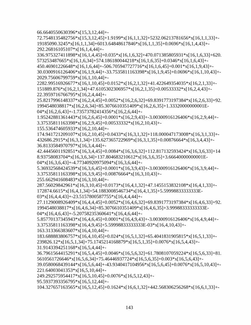
143

66.6640550630396*x[15,3,12,44]+-72.7548135482756*x[15,3,12,45]+1.9199*x[16,1,1,32]+5232.06213781656*x[16,1,1,33]+-19185090.3245*x[16,1,1,34]+6013.64848617846*x[16,1,1,35]+0.0696*x[16,1,4,43]+-292.26816105107*x[16,1,4,44]+-336.975327411898*x[16,1,4,45]+0.035*x[16,1,6,32]+470.071385805931*x[16,1,6,33]+620.573253487665*x[16,1,6,34]+574.186180044218*x[16,1,6,35]+0.0346*x[16,1,6,43]+-450.46901226648*x[16,1,6,44]+-506.705947727716*x[16,1,6,45]+0.001*x[16,1,9,43]+-30.0300916126406*x[16,1,9,44]+-33.7535811163398*x[16,1,9,45]+0.0696*x[16,1,10,43]+-2029.75606799759*x[16,1,10,44]+-2282.99516926677*x[16,1,10,45]+0.0152*x[16,2,1,32]+41.422649354035*x[16,2,1,33]+-151889.876*x[16,2,1,34]+47.6105302306957*x[16,2,1,35]+0.00533332*x[16,2,4,43]+-22.3959716766795*x[16,2,4,44]+-25.8217996148337*x[16,2,4,45]+0.0052*x[16,2,6,32]+69.8391773197384*x[16,2,6,33]+92.1994548038817*x[16,2,6,34]+85.3076610351409*x[16,2,6,35]+1.33320000000001E-04*x[16,2,6,43]+-1.73573782414356*x[16,2,6,44]+-1.95242881361443*x[16,2,6,45]+0.0001*x[16,2,9,43]+-3.00300916126406*x[16,2,9,44]+-3.37535811163398*x[16,2,9,45]+0.00533332*x[16,2,10,43]+-155.536474605933*x[16,2,10,44]+-174.941721209107*x[16,2,10,45]+0.0433*x[16,3,1,32]+118.000047173008*x[16,3,1,33]+-432686.2915*x[16,3,1,34]+135.627365722969*x[16,3,1,35]+0.00876664*x[16,3,4,43]+-36.8133584970797*x[16,3,4,44]+-42.4445601192851*x[16,3,4,45]+0.0084*x[16,3,6,32]+112.817132593424*x[16,3,6,33]+148.93758083704*x[16,3,6,34]+137.804683210612*x[16,3,6,35]+3.66640000000001E-04*x[16,3,6,43]+-4.77340920975094*x[16,3,6,44]+-5.36932568424539*x[16,3,6,45]+0.0001*x[16,3,9,43]+-3.00300916126406*x[16,3,9,44]+-3.37535811163398*x[16,3,9,45]+0.00876664*x[16,3,10,43]+-255.662941608483*x[16,3,10,44]+-287.56029842961*x[16,3,10,45]+0.0173*x[16,4,1,32]+47.1455153832108*x[16,4,1,33]+-172874.6615*x[16,4,1,34]+54.1883008546734*x[16,4,1,35]+5.59998833333333E-03*x[16,4,4,43]+-23.5157800587755*x[16,4,4,44]+-27.1129008926409*x[16,4,4,45]+0.0052*x[16,4,6,32]+69.8391773197384*x[16,4,6,33]+92.1994548038817*x[16,4,6,34]+85.3076610351409*x[16,4,6,35]+3.99988333333333E-04*x[16,4,6,43]+-5.20758235360641*x[16,4,6,44]+-5.85770137345943*x[16,4,6,45]+0.0001*x[16,4,9,43]+-3.00300916126406*x[16,4,9,44]+-3.37535811163398*x[16,4,9,45]+5.59998833333333E-03*x[16,4,10,43]+-163.313366383607*x[16,4,10,44]+-183.688883806757*x[16,4,10,45]+0.024*x[16,5,1,32]+65.4041831905815*x[16,5,1,33]+-239826.12*x[16,5,1,34]+75.1745214168879*x[16,5,1,35]+0.0076*x[16,5,4,43]+-31.9143394251168*x[16,5,4,44]+-36.7961564415291*x[16,5,4,45]+0.0046*x[16,5,6,32]+61.7808107059224*x[16,5,6,33]+81.5610561726646*x[16,5,6,34]+75.46446937724*x[16,5,6,35]+0.003*x[16,5,6,43]+-39.0580068439144*x[16,5,6,44]+-43.9340417104956*x[16,5,6,45]+0.0076*x[16,5,10,43]+-221.64003041353*x[16,5,10,44]+-249.292575954417*x[16,5,10,45]+0.0076*x[16,5,12,43]+-95.5937393356795*x[16,5,12,44]+-104.327657163565*x[16,5,12,45]+0.1624*x[16,6,1,32]+442.568306256268*x[16,6,1,33]+-

144

1622823.412*x[16,6,1,34]+508.680928254275*x[16,6,1,35]+0.0051*x[16,6,4,10]+640.905807887921*x[16,6,4,11]+-50313.795*x[16,6,4,12]+-50313.795*x[16,6,4,13]+-50313.795*x[16,6,4,14]+661.512842387921*x[16,6,4,15]+0.0113*x[16,6,4,43]+-47.4515836189237*x[16,6,4,44]+-54.7100747091156*x[16,6,4,45]+0.0164*x[16,6,6,43]+-213.517104080065*x[16,6,6,44]+-240.172761350709*x[16,6,6,45]+0.0002*x[16,6,9,43]+-6.00601832252813*x[16,6,9,44]+-6.75071622326796*x[16,6,9,45]+0.0164*x[16,6,10,43]+-478.275855102881*x[16,6,10,44]+-537.947137585848*x[16,6,10,45]+0.024*x[16,7,1,32]+65.4041831905815*x[16,7,1,33]+-239826.12*x[16,7,1,34]+75.1745214168879*x[16,7,1,35]+0.003*x[16,7,4,10]+377.00341640466*x[16,7,4,11]+-29596.35*x[16,7,4,12]+-29596.35*x[16,7,4,13]+-29596.35*x[16,7,4,14]+389.12520140466*x[16,7,4,15]+0.0046*x[16,7,4,43]+-19.3165738625707*x[16,7,4,44]+-22.2713578461886*x[16,7,4,45]+0.0046*x[16,7,6,32]+61.7808107059224*x[16,7,6,33]+81.5610561726646*x[16,7,6,34]+75.46446937724*x[16,7,6,35]+0.003*x[16,7,6,43]+-39.0580068439144*x[16,7,6,44]+-43.9340417104956*x[16,7,6,45]+0.0001*x[16,7,9,43]+-3.00300916126406*x[16,7,9,44]+-3.37535811163398*x[16,7,9,45]+0.0076*x[16,7,10,43]+-221.64003041353*x[16,7,10,44]+-249.292575954417*x[16,7,10,45]+0.0076*x[16,7,12,43]+-95.5937393356795*x[16,7,12,44]+-104.327657163565*x[16,7,12,45]+0.0373*x[16,8,1,43]+-133.03851754126*x[16,8,1,44]+-153.404764631253*x[16,8,1,45]+8.06666666666667E-03*x[16,8,4,43]+-33.8739918459573*x[16,8,4,44]+-39.0555695563598*x[16,8,4,45]+0.0001*x[16,8,9,43]+-3.00300916126406*x[16,8,9,44]+-3.37535811163398*x[16,8,9,45]+8.06666666666667E-03*x[16,8,10,43]+-235.249505965238*x[16,8,10,44]+-264.600014828811*x[16,8,10,45]+0.0373*x[16,9,1,43]+-133.03851754126*x[16,9,1,44]+-153.404764631253*x[16,9,1,45]+8.06666666666667E-03*x[16,9,4,43]+-33.8739918459573*x[16,9,4,44]+-39.0555695563598*x[16,9,4,45]+0.0001*x[16,9,9,43]+-3.00300916126406*x[16,9,9,44]+-3.37535811163398*x[16,9,9,45]+8.06666666666667E-03*x[16,9,10,43]+-235.249505965238*x[16,9,10,44]+-264.600014828811*x[16,9,10,45]+1.0971*x[16,10,1,43]+-3913.04443953128*x[16,10,1,44]+-4512.07418973051*x[16,10,1,45]+0.049272105*x[16,10,4,43]+-206.906142521052*x[16,10,4,44]+-238.555800497822*x[16,10,4,45]+0.049272105*x[16,10,6,43]+-641.49007143469*x[16,10,6,44]+-721.57423874464*x[16,10,6,45]+0.0012*x[16,10,9,43]+-36.0361099351688*x[16,10,9,44]+-40.5042973396078*x[16,10,9,45]+0.049272105*x[16,10,10,43]+-1436.93037509719*x[16,10,10,44]+-1616.20657607191*x[16,10,10,45]+0.0379*x[16,11,1,43]+-135.178547314042*x[16,11,1,44]+-155.872401595831*x[16,11,1,45]+0.00825*x[16,11,4,43]+-34.6438552970018*x[16,11,4,44]+-39.9431961371862*x[16,11,4,45]+0.0001*x[16,11,9,43]+-3.00300916126406*x[16,11,9,44]+-3.37535811163398*x[16,11,9,45]+0.00825*x[16,11,10,43]+-240.596085646266*x[16,11,10,44]+-

145

270.613651529466*x[16,11,10,45]+0.0589*x[16,12,1,43]+-210.0795893614*x[16,12,1,44]+-242.239695356054*x[16,12,1,45]+1.02321616666667E-02*x[16,12,4,43]+-42.9674579582459*x[16,12,4,44]+-49.540029134432*x[16,12,4,45]+0.0001*x[16,12,9,43]+-3.00300916126406*x[16,12,9,44]+-3.37535811163398*x[16,12,9,45]+1.02321616666667E-02*x[16,12,10,43]+-298.402187236337*x[16,12,10,44]+-335.631834140181*x[16,12,10,45]+0.0313*x[17,1,2,43]+-112.014943479954*x[17,1,2,44]+-132.933263344193*x[17,1,2,45]+0.0074*x[17,1,7,43]+-125.464371093782*x[17,1,7,44]+-136.971529383214*x[17,1,7,45]+0.0036*x[17,1,8,43]+-59.0788817742593*x[17,1,8,44]+-64.3001099560661*x[17,1,8,45]+0.0074*x[17,1,12,43]+-93.0781146163195*x[17,1,12,44]+-101.582192501366*x[17,1,12,45]+0.0006*x[17,2,1,10]+21.0227455354222*x[17,2,1,11]+-5975.781*x[17,2,1,12]+-5975.781*x[17,2,1,13]+-5975.781*x[17,2,1,14]+21.7513630354222*x[17,2,1,15]+1.6625*x[17,2,1,43]+-5929.6658287492*x[17,2,1,44]+-6837.41075601766*x[17,2,1,45]+0.0615833*x[17,2,4,43]+-258.603991989315*x[17,2,4,44]+-298.161676445476*x[17,2,4,45]+0.0615833*x[17,2,6,43]+-801.773650956945*x[17,2,6,44]+-901.867756956655*x[17,2,6,45]+0.0009*x[17,2,9,43]+-27.0270824513766*x[17,2,9,44]+-30.3782230047058*x[17,2,9,45]+0.0615833*x[17,2,10,43]+-1795.96374802178*x[17,2,10,44]+-2020.03414378601*x[17,2,10,45]+0.2967*x[17,3,1,43]+-1058.24472264053*x[17,3,1,44]+-1220.24647898372*x[17,3,1,45]+0.021316*x[17,3,4,43]+-89.5113235770775*x[17,3,4,44]+-103.203535619425*x[17,3,4,45]+0.021316*x[17,3,6,43]+-277.520157961626*x[17,3,6,44]+-312.166011033642*x[17,3,6,45]+0.0002*x[17,3,9,43]+-6.00601832252813*x[17,3,9,44]+-6.75071622326796*x[17,3,9,45]+0.021316*x[17,3,10,43]+-621.641958986159*x[17,3,10,44]+-699.200072242679*x[17,3,10,45]+1.4863*x[18,1,1,32]+4050.42656150672*x[18,1,1,33]+-14852231.7565*x[18,1,1,34]+4655.49546591336*x[18,1,1,35]+0.01*x[18,1,4,10]+1256.6780546822*x[18,1,4,11]+-98654.5*x[18,1,4,12]+-98654.5*x[18,1,4,13]+-98654.5*x[18,1,4,14]+1297.0840046822*x[18,1,4,15]+0.0061*x[18,1,4,21]+259.347861140387*x[18,1,4,22]+-60684.325*x[18,1,4,23]+-60684.325*x[18,1,4,24]+286.141242856141*x[18,1,4,25]+0.03876602*x[18,1,4,43]+-162.788410584324*x[18,1,4,44]+-187.68954428098*x[18,1,4,45]+0.0008*x[18,1,9,43]+-24.0240732901125*x[18,1,9,44]+-27.0028648930719*x[18,1,9,45]+0.05486602*x[18,1,10,43]+-1600.06662387755*x[18,1,10,44]+-1799.6962444956*x[18,1,10,45]+0.0504*x[18,2,1,32]+137.348784700221*x[18,2,1,33]+-503634.852*x[18,2,1,34]+157.866494975465*x[18,2,1,35]+0.001*x[18,2,4,10]+125.66780546822*x[18,2,4,11]+-9865.45*x[18,2,4,12]+-9865.45*x[18,2,4,13]+-9865.45*x[18,2,4,14]+129.70840046822*x[18,2,4,15]+7.06651833333333E-03*x[18,2,4,43]+-29.6741137689224*x[18,2,4,44]+-34.2132518539824*x[18,2,4,45]+0.0001*x[18,2,9,43]+-3.00300916126406*x[18,2,9,44]+-

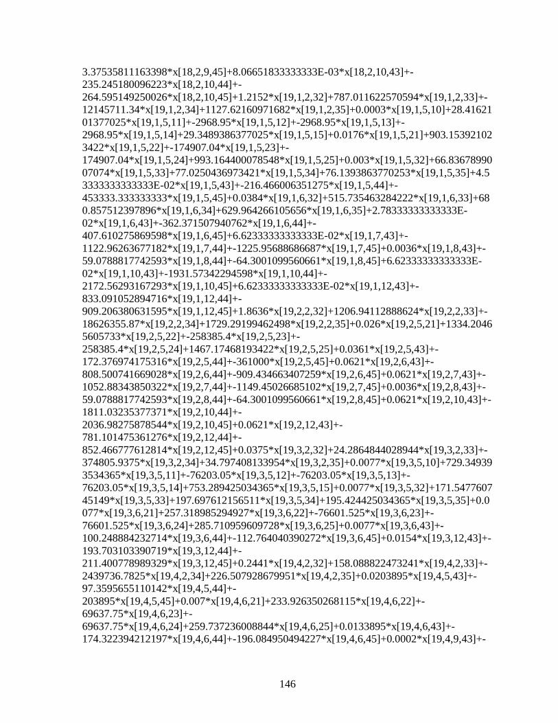
146

3.37535811163398*x[18,2,9,45]+8.06651833333333E-03*x[18,2,10,43]+-235.245180096223*x[18,2,10,44]+-264.595149250026*x[18,2,10,45]+1.2152*x[19,1,2,32]+787.011622570594*x[19,1,2,33]+-12145711.34*x[19,1,2,34]+1127.62160971682*x[19,1,2,35]+0.0003*x[19,1,5,10]+28.4162101377025*x[19,1,5,11]+-2968.95*x[19,1,5,12]+-2968.95*x[19,1,5,13]+-2968.95*x[19,1,5,14]+29.3489386377025*x[19,1,5,15]+0.0176*x[19,1,5,21]+903.153921023422*x[19,1,5,22]+-174907.04*x[19,1,5,23]+-174907.04*x[19,1,5,24]+993.164400078548*x[19,1,5,25]+0.003*x[19,1,5,32]+66.8367899007074*x[19,1,5,33]+77.0250436973421*x[19,1,5,34]+76.1393863770253*x[19,1,5,35]+4.53333333333333E-02*x[19,1,5,43]+-216.466006351275*x[19,1,5,44]+-453333.333333333*x[19,1,5,45]+0.0384*x[19,1,6,32]+515.735463284222*x[19,1,6,33]+680.857512397896*x[19,1,6,34]+629.964266105656*x[19,1,6,35]+2.78333333333333E-02*x[19,1,6,43]+-362.371507940762*x[19,1,6,44]+-407.610275869598*x[19,1,6,45]+6.62333333333333E-02*x[19,1,7,43]+-1122.96263677182*x[19,1,7,44]+-1225.95688686687*x[19,1,7,45]+0.0036*x[19,1,8,43]+-59.0788817742593*x[19,1,8,44]+-64.3001099560661*x[19,1,8,45]+6.62333333333333E-02*x[19,1,10,43]+-1931.57342294598*x[19,1,10,44]+-2172.56293167293*x[19,1,10,45]+6.62333333333333E-02*x[19,1,12,43]+-833.091052894716*x[19,1,12,44]+-909.206380631595*x[19,1,12,45]+1.8636*x[19,2,2,32]+1206.94112888624*x[19,2,2,33]+-18626355.87*x[19,2,2,34]+1729.29199462498*x[19,2,2,35]+0.026*x[19,2,5,21]+1334.20465605733*x[19,2,5,22]+-258385.4*x[19,2,5,23]+-258385.4*x[19,2,5,24]+1467.17468193422*x[19,2,5,25]+0.0361*x[19,2,5,43]+-172.376974175316*x[19,2,5,44]+-361000*x[19,2,5,45]+0.0621*x[19,2,6,43]+-808.500741669028*x[19,2,6,44]+-909.434663407259*x[19,2,6,45]+0.0621*x[19,2,7,43]+-1052.88343850322*x[19,2,7,44]+-1149.45026685102*x[19,2,7,45]+0.0036*x[19,2,8,43]+-59.0788817742593*x[19,2,8,44]+-64.3001099560661*x[19,2,8,45]+0.0621*x[19,2,10,43]+-1811.03235377371*x[19,2,10,44]+-2036.98275878544*x[19,2,10,45]+0.0621*x[19,2,12,43]+-781.101475361276*x[19,2,12,44]+-852.466777612814*x[19,2,12,45]+0.0375*x[19,3,2,32]+24.2864844028944*x[19,3,2,33]+-374805.9375*x[19,3,2,34]+34.797408133954*x[19,3,2,35]+0.0077*x[19,3,5,10]+729.349393534365*x[19,3,5,11]+-76203.05*x[19,3,5,12]+-76203.05*x[19,3,5,13]+-76203.05*x[19,3,5,14]+753.289425034365*x[19,3,5,15]+0.0077*x[19,3,5,32]+171.547760745149*x[19,3,5,33]+197.697612156511*x[19,3,5,34]+195.424425034365*x[19,3,5,35]+0.0077*x[19,3,6,21]+257.318985294927*x[19,3,6,22]+-76601.525*x[19,3,6,23]+-76601.525*x[19,3,6,24]+285.710959609728*x[19,3,6,25]+0.0077*x[19,3,6,43]+-100.248884232714*x[19,3,6,44]+-112.764040390272*x[19,3,6,45]+0.0154*x[19,3,12,43]+-193.703103390719*x[19,3,12,44]+-211.400778989329*x[19,3,12,45]+0.2441*x[19,4,2,32]+158.088822473241*x[19,4,2,33]+-2439736.7825*x[19,4,2,34]+226.507928679951*x[19,4,2,35]+0.0203895*x[19,4,5,43]+-97.3595655110142*x[19,4,5,44]+-203895*x[19,4,5,45]+0.007*x[19,4,6,21]+233.926350268115*x[19,4,6,22]+-69637.75*x[19,4,6,23]+-69637.75*x[19,4,6,24]+259.737236008844*x[19,4,6,25]+0.0133895*x[19,4,6,43]+-174.322394212197*x[19,4,6,44]+-196.084950494227*x[19,4,6,45]+0.0002*x[19,4,9,43]+-

147

6.00601832252813*x[19,4,9,44]+-6.75071622326796*x[19,4,9,45]+0.0203895*x[19,4,12,43]+-256.461651076952*x[19,4,12,44]+-279.893258649541*x[19,4,12,45]+0.1156*x[19,5,1,32]+315.030149034634*x[19,5,1,33]+-1155162.478*x[19,5,1,34]+362.090611491344*x[19,5,1,35]+0.0136*x[19,5,4,43]+-57.109870550209*x[19,5,4,44]+-65.8457536322099*x[19,5,4,45]+0.0018*x[19,5,6,21]+60.152490068944*x[19,5,6,22]+-17906.85*x[19,5,6,23]+-17906.85*x[19,5,6,24]+66.7895749737026*x[19,5,6,25]+0.0118*x[19,5,6,43]+-153.62816025273*x[19,5,6,44]+-172.807230727949*x[19,5,6,45]+0.0036*x[19,5,8,43]+-59.0788817742593*x[19,5,8,44]+-64.3001099560661*x[19,5,8,45]+0.0136*x[19,5,12,43]+-171.062480916479*x[19,5,12,44]+-186.691597029537*x[19,5,12,45]+0.777*x[20,1,1,43]+-2771.33855575226*x[20,1,1,44]+-3195.58986912825*x[20,1,1,45]+4.20833333333333E-02*x[20,1,4,43]+-176.718655807938*x[20,1,4,44]+-203.750646962414*x[20,1,4,45]+0.0004*x[20,1,9,43]+-12.0120366450563*x[20,1,9,44]+-13.5014324465359*x[20,1,9,45]+0.008*x[20,1,12,32]+122.258725127125*x[20,1,12,33]+145.375011225601*x[20,1,12,34]+138.581413512037*x[20,1,12,35]+3.40833333333333E-02*x[20,1,12,43]+-428.704379257598*x[20,1,12,44]+-467.872936183093*x[20,1,12,45]+0.1071*x[20,2,1,43]+-381.995314441528*x[20,2,1,44]+-440.473198177138*x[20,2,1,45]+0.0006*x[20,2,4,21]+25.5096256859397*x[20,2,4,22]+-5968.95*x[20,2,4,23]+-5968.95*x[20,2,4,24]+28.1450402809319*x[20,2,4,25]+0.02875*x[20,2,4,43]+-120.728586641067*x[20,2,4,44]+-139.195986538679*x[20,2,4,45]+0.0002*x[20,2,9,43]+-6.00601832252813*x[20,2,9,44]+-6.75071622326796*x[20,2,9,45]+0.0006*x[20,2,11,21]+13.5998943724423*x[20,2,11,22]+-5981.37*x[20,2,11,23]+-5981.37*x[20,2,11,24]+16.4171018159342*x[20,2,11,25]+0.02875*x[20,2,11,43]+-95.7245574905882*x[20,2,11,44]+-106.034704653151*x[20,2,11,45]+0.0014*x[20,2,12,21]+131.123210175898*x[20,2,12,22]+-13840.61*x[20,2,12,23]+-13840.61*x[20,2,12,24]+140.171747364606*x[20,2,12,25]+0.0014*x[20,2,12,32]+21.3952768972469*x[20,2,12,33]+25.4406269644801*x[20,2,12,34]+24.2517473646064*x[20,2,12,35]+0.02655*x[20,2,12,43]+-333.949181495038*x[20,2,12,44]+-364.460433906928*x[20,2,12,45]+0.5586*x[20,3,1,43]+-1992.36771845973*x[20,3,1,44]+-2297.37001402193*x[20,3,1,45]+0.03495*x[20,3,4,43]+-146.763968803662*x[20,3,4,44]+-169.213903635716*x[20,3,4,45]+0.0002*x[20,3,9,43]+-6.00601832252813*x[20,3,9,44]+-6.75071622326796*x[20,3,9,45]+0.03495*x[20,3,11,43]+-116.367766410298*x[20,3,11,44]+-128.90131922183*x[20,3,11,45]+0.002*x[20,3,12,21]+187.318871679854*x[20,3,12,22]+-19772.3*x[20,3,12,23]+-19772.3*x[20,3,12,24]+200.245353378009*x[20,3,12,25]+0.002*x[20,3,12,32]+30.5646812817813*x[20,3,12,33]+36.3437528064001*x[20,3,12,34]+34.6453533780092*x[20,3,12,35]+0.03095*x[20,3,12,43]+-389.292925320958*x[20,3,12,44]+-424.860656475308*x[20,3,12,45]+0.0806*x[20,4,1,43]+-287.477332810337*x[20,4,1,44]+-331.485898908285*x[20,4,1,45]+0.0133*x[20,4,4,43]+-55.8500939939544*x[20,4,4,44]+-64.3932737726759*x[20,4,4,45]+0.0001*x[20,4,9,43]+-3.00300916126406*x[20,4,9,44]+-

148

3.37535811163398*x[20,4,9,45]+0.0133*x[20,4,11,43]+-44.2830126826025*x[20,4,11,44]+-49.0525764134576*x[20,4,11,45]+0.0008*x[20,4,12,21]+74.9275486719418*x[20,4,12,22]+-7908.92*x[20,4,12,23]+-7908.92*x[20,4,12,24]+80.0981413512037*x[20,4,12,25]+0.0008*x[20,4,12,32]+12.2258725127125*x[20,4,12,33]+14.5375011225601*x[20,4,12,34]+13.8581413512037*x[20,4,12,35]+0.0117*x[20,4,12,43]+-147.164046082559*x[20,4,12,44]+-160.609682738646*x[20,4,12,45]+0.2019*x[21,1,2,32]+130.758432025183*x[21,1,2,33]+-2017955.1675*x[21,1,2,34]+187.349245393208*x[21,1,2,35]+0.0004*x[21,1,5,10]+37.8882801836034*x[21,1,5,11]+-3958.6*x[21,1,5,12]+-3958.6*x[21,1,5,13]+-3958.6*x[21,1,5,14]+39.1319181836034*x[21,1,5,15]+0.0025*x[21,1,5,21]+128.288909236282*x[21,1,5,22]+-24844.75*x[21,1,5,23]+-24844.75*x[21,1,5,24]+141.074488647521*x[21,1,5,25]+0.034*x[21,1,5,32]+757.483618874684*x[21,1,5,33]+872.950495236544*x[21,1,5,34]+862.913045606287*x[21,1,5,35]+0.0031*x[21,1,5,43]+-14.8024548460798*x[21,1,5,44]+-31000*x[21,1,5,45]+0.0016*x[21,1,6,32]+21.4889776368426*x[21,1,6,33]+28.369063016579*x[21,1,6,34]+26.2485110877357*x[21,1,6,35]+0.0384*x[21,1,6,43]+-499.942487602104*x[21,1,6,44]+-562.355733894344*x[21,1,6,45]+0.0002*x[21,1,9,43]+-6.00601832252813*x[21,1,9,44]+-6.75071622326796*x[21,1,9,45]+0.04*x[21,1,10,43]+-1166.52647586068*x[21,1,10,44]+-1312.06618923378*x[21,1,10,45]+0.0229*x[21,2,2,32]+14.8309464753675*x[21,2,2,33]+-228881.4925*x[21,2,2,34]+21.2496172338012*x[21,2,2,35]+0.006466*x[21,2,5,43]+-30.8750558176619*x[21,2,5,44]+-64660*x[21,2,5,45]+0.006466*x[21,2,6,43]+-84.1830240842502*x[21,2,6,44]+-94.6925045666882*x[21,2,6,45]+0.0036*x[21,2,8,43]+-59.0788817742593*x[21,2,8,44]+-64.3001099560661*x[21,2,8,45]+0.006466*x[21,2,10,43]+-188.56900482288*x[21,2,10,44]+-212.09549948964*x[21,2,10,45]+1.1706*x[21,3,2,32]+758.126897120751*x[21,3,2,33]+-11699942.145*x[21,3,2,34]+1086.23589230951*x[21,3,2,35]+0.0798*x[21,3,5,21]+4094.98198282211*x[21,3,5,22]+-793044.42*x[21,3,5,23]+-793044.42*x[21,3,5,24]+4503.09767762887*x[21,3,5,25]+0.0798*x[21,3,6,43]+-1038.94298204812*x[21,3,6,44]+-1168.64550949918*x[21,3,6,45]+0.0006*x[21,3,9,43]+-18.0180549675844*x[21,3,9,44]+-20.2521486698039*x[21,3,9,45]+0.0798*x[21,3,10,43]+-2327.22031934207*x[21,3,10,44]+-2617.57204752138*x[21,3,10,45]+0.3902*x[21,4,2,32]+252.708965706917*x[21,4,2,33]+-3899980.715*x[21,4,2,34]+362.078630769836*x[21,4,2,35]+0.025246*x[21,4,5,43]+-120.5492822723*x[21,4,5,44]+-252460*x[21,4,5,45]+0.025246*x[21,4,6,43]+-328.686146927154*x[21,4,6,44]+-369.719605674391*x[21,4,6,45]+0.0001*x[21,4,9,43]+-3.00300916126406*x[21,4,9,44]+-3.37535811163398*x[21,4,9,45]+0.0053*x[21,4,10,10]+198.594976426525*x[21,4,10,11]+-52616.015*x[21,4,10,12]+-52616.015*x[21,4,10,13]+-52616.015*x[21,4,10,14]+210.136229926525*x[21,4,10,15]+0.019946*x[21,4,10,43]+-581.688427187931*x[21,4,10,44]+-654.261805261422*x[21,4,10,45]+0.0369*x[21,5,2,32]+23.8979006524481*x[21,5,2,33]+-368809.0425*x[21,5,2,34]+34.2406496038107*x[21,5,2,35]+0.0099*x[21,5,5,21]+508.024080575675*x[21,5,5,22]+-98385.21*x[21,5,5,23]+-

149

98385.21*x[21,5,5,24]+558.654975044184*x[21,5,5,25]+0.008*x[21,5,5,32]+178.23143973522*x[21,5,5,33]+205.400116526246*x[21,5,5,34]+203.038363672067*x[21,5,5,35]+0.0019*x[21,5,6,10]+220.147644716686*x[21,5,6,11]+-18744.355*x[21,5,6,12]+-18744.355*x[21,5,6,13]+-18744.355*x[21,5,6,14]+227.820106916686*x[21,5,6,15]+0.0038*x[21,5,6,21]+126.988590145548*x[21,5,6,22]+-37803.35*x[21,5,6,23]+-37803.35*x[21,5,6,24]+141.000213833372*x[21,5,6,25]+0.0122*x[21,5,6,43]+-158.835894498585*x[21,5,6,44]+-178.665102956016*x[21,5,6,45]+0.0001*x[21,5,9,43]+-3.00300916126406*x[21,5,9,44]+-3.37535811163398*x[21,5,9,45]+0.0179*x[21,5,10,43]+-522.020597947657*x[21,5,10,44]+-587.149619682114*x[21,5,10,45]+0.0267*x[21,6,2,32]+17.2919768948608*x[21,6,2,33]+-266861.8275*x[21,6,2,34]+24.7757545913752*x[21,6,2,35]+0.0068*x[21,6,5,32]+151.496723774937*x[21,6,5,33]+174.590099047309*x[21,6,5,34]+172.582609121257*x[21,6,5,35]+0.0014*x[21,6,6,21]+46.7852700536231*x[21,6,6,22]+-13927.55*x[21,6,6,23]+-13927.55*x[21,6,6,24]+51.9474472017687*x[21,6,6,25]+0.0054*x[21,6,6,43]+-70.3044123190459*x[21,6,6,44]+-79.0812750788921*x[21,6,6,45]+0.0001*x[21,6,9,43]+-3.00300916126406*x[21,6,9,44]+-3.37535811163398*x[21,6,9,45]+0.0068*x[21,6,10,43]+-198.309500896316*x[21,6,10,44]+-223.051252169742*x[21,6,10,45]+0.0358*x[22,1,7,43]+-606.976281778025*x[22,1,7,44]+-662.646047556629*x[22,1,7,45]+0.0048*x[22,1,8,43]+-78.7718423656791*x[22,1,8,44]+-85.7334799414214*x[22,1,8,45]+0.597*x[22,1,14,43]+-3006.37381587333*x[22,1,14,44]+-6203.5696499677*x[22,1,14,45]+0.1295*x[23,1,2,32]+83.8693261379953*x[23,1,2,33]+-1294329.8375*x[23,1,2,34]+120.167049422588*x[23,1,2,35]+0.0001*x[23,1,9,43]+-3.00300916126406*x[23,1,9,44]+-3.37535811163398*x[23,1,9,45]+0.003*x[23,1,12,21]+280.978307519782*x[23,1,12,22]+-29658.45*x[23,1,12,23]+-29658.45*x[23,1,12,24]+300.368030067014*x[23,1,12,25]+0.01503034*x[23,1,12,43]+-189.053474221926*x[23,1,12,44]+-206.326336654187*x[23,1,12,45]+0.8215*x[23,2,2,32]+532.035918319406*x[23,2,2,33]+-8210748.7375*x[23,2,2,34]+762.295220854485*x[23,2,2,35]+0.0474597*x[23,2,5,43]+-226.619376212417*x[23,2,5,44]+-474597*x[23,2,5,45]+0.0474597*x[23,2,6,43]+-617.893762470042*x[23,2,6,44]+-695.03214645587*x[23,2,6,45]+0.0005*x[23,2,9,43]+-15.0150458063203*x[23,2,9,44]+-16.8767905581699*x[23,2,9,45]+0.0474597*x[23,2,10,43]+-1384.07491466013*x[23,2,10,44]+-1556.75669302945*x[23,2,10,45]+0.0099*x[23,3,2,32]+6.41163188236412*x[23,3,2,33]+-98948.7675*x[23,3,2,34]+9.18651574736385*x[23,3,2,35]+0.004042*x[23,3,5,43]+-19.3004911251144*x[23,3,5,44]+-40420*x[23,3,5,45]+0.004042*x[23,3,10,43]+-117.877500385722*x[23,3,10,44]+-132.584288422073*x[23,3,10,45]+0.004042*x[23,3,12,43]+-50.8407755782653*x[23,3,12,44]+-55.4858408230434*x[23,3,12,45]+0.0099*x[23,4,2,32]+6.41163188236412*x[23,4,2,33]+-98948.7675*x[23,4,2,34]+9.18651574736385*x[23,4,2,35]+0.004042*x[23,4,5,43]+-19.3004911251144*x[23,4,5,44]+-40420*x[23,4,5,45]+0.004042*x[23,4,12,43]+-50.8407755782653*x[23,4,12,44]+-55.4858408230434*x[23,4,12,45]+0.0885*x[23,5,2,32]+57.3161031908308*x[23,5,2,33]+-

150

884542.0125*x[23,5,2,34]+82.1218831961314*x[23,5,2,35]+0.01383232*x[23,5,5,43]+-66.0491265214602*x[23,5,5,44]+-138323.2*x[23,5,5,45]+0.01383232*x[23,5,6,43]+-180.087616409071*x[23,5,6,44]+-202.569907944308*x[23,5,6,45]+0.01383232*x[23,5,10,43]+-403.394187564432*x[23,5,10,44]+-453.722984766553*x[23,5,10,45]+0.005*x[24,1,2,10]+174.517841917861*x[24,1,2,11]+-49798.175*x[24,1,2,12]+-49798.175*x[24,1,2,13]+-49798.175*x[24,1,2,14]+180.589654417861*x[24,1,2,15]+0.1402*x[24,1,2,32]+90.7990696876212*x[24,1,2,33]+-1401274.465*x[24,1,2,34]+130.095909876809*x[24,1,2,35]+0.01911666*x[24,1,5,43]+-91.2817730509226*x[24,1,5,44]+-191166.6*x[24,1,5,45]+0.01911666*x[24,1,6,43]+-248.886212370928*x[24,1,6,44]+-279.957379268454*x[24,1,6,45]+0.01911666*x[24,1,10,43]+-557.502250500673*x[24,1,10,44]+-627.058080926944*x[24,1,10,45]+0.005*x[24,2,2,21]+86.2903775708823*x[24,2,2,22]+-49886.15*x[24,2,2,23]+-49886.15*x[24,2,2,24]+92.6146544178605*x[24,2,2,25]+0.2622*x[24,2,2,32]+169.811098945038*x[24,2,2,33]+-2620643.115*x[24,2,2,34]+243.303477672606*x[24,2,2,35]+0.0078*x[24,2,5,10]+738.821463580266*x[24,2,5,11]+-77192.7*x[24,2,5,12]+-77192.7*x[24,2,5,13]+-77192.7*x[24,2,5,14]+763.072404580266*x[24,2,5,15]+0.01467036*x[24,2,5,43]+-70.0507553147533*x[24,2,5,44]+-146703.6*x[24,2,5,45]+0.02247036*x[24,2,6,43]+-292.54915822174*x[24,2,6,44]+-329.071244496618*x[24,2,6,45]+0.0003*x[24,2,9,43]+-9.00902748379219*x[24,2,9,44]+-10.1260743349019*x[24,2,9,45]+0.02247036*x[24,2,10,43]+-655.306746553023*x[24,2,10,44]+-737.064990397776*x[24,2,10,45]+0.3047*x[24,3,1,54]+-864.391124533792*x[24,3,2,55]+0.02191668*x[24,3,4,43]+-92.0337321831143*x[24,3,4,44]+-106.111787626175*x[24,3,4,45]+0.02191668*x[24,3,6,43]+-285.340612478627*x[24,3,6,44]+-320.962777758528*x[24,3,6,45]+0.02191668*x[24,3,7,43]+-371.589523332927*x[24,3,7,44]+-405.670429540877*x[24,3,7,45]+0.0024*x[24,3,8,43]+-39.3859211828396*x[24,3,8,44]+-42.8667399707107*x[24,3,8,45]+0.0004*x[24,3,9,43]+-12.0120366450563*x[24,3,9,44]+-13.5014324465359*x[24,3,9,45]+0.02191668*x[24,3,10,43]+-639.159687074159*x[24,3,10,44]+-718.903370206402*x[24,3,10,45]+0.02191668*x[24,3,12,43]+-275.670709871513*x[24,3,12,44]+-300.857352263627*x[24,3,12,45]+0.0422*x[24,4,1,32]+115.002355443439*x[24,4,1,33]+-421694.261*x[24,4,1,34]+132.181866824695*x[24,4,1,35]+0.0118*x[24,4,4,43]+-49.5512112126813*x[24,4,4,44]+-57.1308744750057*x[24,4,4,45]+0.0118*x[24,4,6,43]+-153.62816025273*x[24,4,6,44]+-172.807230727949*x[24,4,6,45]+0.0093*x[24,5,1,32]+25.3441209863503*x[24,5,1,33]+-92932.6215*x[24,5,1,34]+29.1301270490441*x[24,5,1,35]+0.0053*x[24,5,4,43]+-22.2560524938314*x[24,5,4,44]+-

151

25.6604775184347*x[24,5,4,45]+0.0012*x[24,5,6,21]+40.1016600459626*x[24,5,6,22]+-11937.9*x[24,5,6,23]+-11937.9*x[24,5,6,24]+44.5263833158018*x[24,5,6,25]+0.0041*x[24,5,6,43]+-53.3792760200164*x[24,5,6,44]+-60.0431903376774*x[24,5,6,45]+0.01*x[25,1,2,21]+172.580755141765*x[25,1,2,22]+-99772.3*x[25,1,2,23]+-99772.3*x[25,1,2,24]+185.229308835721*x[25,1,2,25]+1.5348*x[25,1,2,43]+-5492.66885792439*x[25,1,2,44]+-6518.40167989353*x[25,1,2,45]+6.55219783333333E-02*x[25,1,4,43]+-275.14350741252*x[25,1,4,44]+-317.231179619975*x[25,1,4,45]+6.55219783333333E-02*x[25,1,6,43]+-853.052626056715*x[25,1,6,44]+-959.548443016953*x[25,1,6,45]+0.001*x[25,1,9,43]+-30.0300916126406*x[25,1,9,44]+-33.7535811163398*x[25,1,9,45]+6.55219783333333E-02*x[25,1,10,43]+-1910.82806191509*x[25,1,10,44]+-2149.22931057187*x[25,1,10,45]+0.0276*x[25,2,2,43]+-98.7735603848795*x[25,2,2,44]+-117.21910761341*x[25,2,2,45]+0.0082*x[25,2,4,10]+1030.4760048394*x[25,2,4,11]+-80896.69*x[25,2,4,12]+-80896.69*x[25,2,4,13]+-80896.69*x[25,2,4,14]+1063.6088838394*x[25,2,4,15]+0.0082*x[25,2,6,43]+-106.758552040033*x[25,2,6,44]+-120.086380675355*x[25,2,6,45]+0.0001*x[25,2,9,43]+-3.00300916126406*x[25,2,9,44]+-3.37535811163398*x[25,2,9,45]+0.0082*x[25,2,10,43]+-239.13792755144*x[25,2,10,44]+-268.973568792924*x[25,2,10,45]+0.0123*x[25,3,2,43]+-44.0186519106528*x[25,3,2,44]+-52.2389501320631*x[25,3,2,45]+0.0044*x[25,3,4,10]+552.938344060167*x[25,3,4,11]+-43407.98*x[25,3,4,12]+-43407.98*x[25,3,4,13]+-43407.98*x[25,3,4,14]+570.716962060167*x[25,3,4,15]+0.0044*x[25,3,6,43]+-57.2850767044078*x[25,3,6,44]+-64.4365945087269*x[25,3,6,45]+0.0001*x[25,3,9,43]+-3.00300916126406*x[25,3,9,44]+-3.37535811163398*x[25,3,9,45]+0.0044*x[25,3,10,43]+-128.317912344675*x[25,3,10,44]+-144.327280815715*x[25,3,10,45]+0.6572*x[25,4,1,43]+-2344.04594445352*x[25,4,1,44]+-2702.88502186755*x[25,4,1,45]+0.0001*x[25,4,4,10]+12.566780546822*x[25,4,4,11]+-986.545*x[25,4,4,12]+-986.545*x[25,4,4,13]+-986.545*x[25,4,4,14]+12.970840046822*x[25,4,4,15]+4.51252666666667E-02*x[25,4,4,43]+-189.492510138014*x[25,4,4,44]+-218.478469964787*x[25,4,4,45]+0.0006*x[25,4,9,43]+-18.0180549675844*x[25,4,9,44]+-20.2521486698039*x[25,4,9,45]+4.52252666666667E-02*x[25,4,10,43]+-1318.91177361316*x[25,4,10,44]+-1483.46358231037*x[25,4,10,45]+4.52252666666667E-02*x[25,4,11,43]+-150.579778749931*x[25,4,11,44]+-166.798184134261*x[25,4,11,45]+1.1252*x[25,5,2,54]+-2859.85260848753*x[25,5,3,55]+4.99810766666667E-02*x[25,5,4,43]+-209.883295470103*x[25,5,4,44]+-241.988357387201*x[25,5,4,45]+0.0008*x[25,5,9,43]+-24.0240732901125*x[25,5,9,44]+-27.0028648930719*x[25,5,9,45]+4.99810766666667E-02*x[25,5,10,43]+-1457.60623059223*x[25,5,10,44]+-1639.46201989586*x[25,5,10,45]+4.99810766666667E-02*x[25,5,11,43]+-166.414485106777*x[25,5,11,44]+-184.33838965553*x[25,5,11,45]+0.006*x[25,6,1,43]+-21.4002977278167*x[25,6,1,44]+-24.676369645778*x[25,6,1,45]+4.07790333333333E-03*x[25,6,12,43]+-51.2923721424691*x[25,6,12,44]+-55.9786974876525*x[25,6,12,45]+0.0091*x[25,7,1,43]+-32.4571182205219*x[25,7,1,44]+-

152

37.4258272960967*x[25,7,1,45]+0.00442766*x[25,7,12,43]+-55.6916547246072*x[25,7,12,44]+-60.7799203311619*x[25,7,12,45]+0.0224*x[25,8,2,32]+14.5071266833289*x[25,8,2,33]+-223884.08*x[25,8,2,34]+20.7856517920152*x[25,8,2,35]+0.0064*x[25,8,5,10]+606.212482937654*x[25,8,5,11]+-63337.6*x[25,8,5,12]+-63337.6*x[25,8,5,13]+-63337.6*x[25,8,5,14]+626.110690937654*x[25,8,5,15]+3.86346666666667E-04*x[25,8,5,43]+-1.84479970589251*x[25,8,5,44]+-3863.46666666667*x[25,8,5,45]+0.0032*x[25,8,6,21]+106.937760122567*x[25,8,6,22]+-31834.4*x[25,8,6,23]+-31834.4*x[25,8,6,24]+118.737022175471*x[25,8,6,25]+3.58634666666667E-03*x[25,8,6,43]+-46.6918508837721*x[25,8,6,44]+-52.5209013472101*x[25,8,6,45]+0.0048*x[25,8,8,43]+-78.7718423656791*x[25,8,8,44]+-85.7334799414214*x[25,8,8,45]+0.0001*x[25,8,9,43]+-3.00300916126406*x[25,8,9,44]+-3.37535811163398*x[25,8,9,45]+6.78634666666667E-03*x[25,8,10,43]+-197.911326525889*x[25,8,10,44]+-222.603400243817*x[25,8,10,45]+0.0242*x[26,1,1,32]+65.949218050503*x[26,1,1,33]+-241824.671*x[26,1,1,34]+75.8009757620287*x[26,1,1,35]+0.3289*x[26,1,1,43]+-1173.09298711315*x[26,1,1,44]+-1352.67632941606*x[26,1,1,45]+2.38817666666667E-02*x[26,1,4,43]+-100.285632562032*x[26,1,4,44]+-115.625950311416*x[26,1,4,45]+2.38817666666667E-02*x[26,1,6,43]+-310.924735303811*x[26,1,6,44]+-349.740844284552*x[26,1,6,45]+0.0024*x[26,1,8,43]+-39.3859211828396*x[26,1,8,44]+-42.8667399707107*x[26,1,8,45]+2.38817666666667E-02*x[26,1,10,43]+-696.467827674846*x[26,1,10,44]+-783.361464562588*x[26,1,10,45]+0.0026*x[26,2,1,32]+7.08545317897967*x[26,2,1,33]+-25981.163*x[26,2,1,34]+8.14390648682953*x[26,2,1,35]+0.0381*x[26,2,1,43]+-135.891890571636*x[26,2,1,44]+-156.69494725069*x[26,2,1,45]+0.008015105*x[26,2,4,43]+-33.6574712497304*x[26,2,4,44]+-38.8059286151687*x[26,2,4,45]+0.008015105*x[26,2,6,43]+-104.351341981564*x[26,2,6,44]+-117.378652461334*x[26,2,6,45]+0.0024*x[26,2,8,43]+-39.3859211828396*x[26,2,8,44]+-42.8667399707107*x[26,2,8,45]+0.008015105*x[26,2,10,43]+-233.745804732584*x[26,2,10,44]+-262.908706841464*x[26,2,10,45]+1.6079*x[27,1,2,32]+1041.3396872377*x[27,1,2,33]+-16070679.1175*x[27,1,2,34]+1492.02006769559*x[27,1,2,35]+0.0188*x[27,1,5,10]+1780.74916862936*x[27,1,5,11]+-186054.2*x[27,1,5,12]+-186054.2*x[27,1,5,13]+-186054.2*x[27,1,5,14]+1839.20015462936*x[27,1,5,15]+0.0548*x[27,1,5,32]+1220.88536218626*x[27,1,5,33]+1406.99079820478*x[27,1,5,34]+1390.81279115366*x[27,1,5,35]+4.34000000000003E-04*x[27,1,5,43]+-2.07234367845119*x[27,1,5,44]+-4340.00000000003*x[27,1,5,45]+0.056*x[27,1,6,21]+1871.41080214492*x[27,1,6,22]+-557102*x[27,1,6,23]+-557102*x[27,1,6,24]+2077.89788807075*x[27,1,6,25]+0.018034*x[27,1,6,43]+-234.790698474384*x[27,1,6,44]+-264.102169402359*x[27,1,6,45]+0.074034*x[27,1,7,43]+-1255.22016885906*x[27,1,7,44]+-1370.34462248066*x[27,1,7,45]+0.0048*x[27,1,8,43]+-78.7718423656791*x[27,1,8,44]+-

153

85.7334799414214*x[27,1,8,45]+0.074034*x[27,1,10,43]+-2159.06552784675*x[27,1,10,44]+-2428.43770634333*x[27,1,10,45]+0.0207*x[27,1,12,21]+1938.75032188649*x[27,1,12,22]+-204643.305*x[27,1,12,23]+-204643.305*x[27,1,12,24]+2072.5394074624*x[27,1,12,25]+0.053334*x[27,1,12,43]+-670.841643911728*x[27,1,12,44]+-732.133061468629*x[27,1,12,45]+0.5809*x[27,2,2,32]+376.213834390436*x[27,2,2,33]+-5805993.8425*x[27,2,2,34]+539.035050267036*x[27,2,2,35]+0.0225*x[27,2,5,32]+501.275924255305*x[27,2,5,33]+577.687827730066*x[27,2,5,34]+571.04539782769*x[27,2,5,35]+0.011648*x[27,2,5,43]+-55.6190303377863*x[27,2,5,44]+-116480*x[27,2,5,45]+0.034148*x[27,2,6,43]+-444.584272568663*x[27,2,6,44]+-500.086552110002*x[27,2,6,45]+0.034148*x[27,2,7,43]+-578.967208663575*x[27,2,7,44]+-632.068079105133*x[27,2,7,45]+0.0048*x[27,2,8,43]+-78.7718423656791*x[27,2,8,44]+-85.7334799414214*x[27,2,8,45]+0.034148*x[27,2,10,43]+-995.863652442267*x[27,2,10,44]+-1120.11090574887*x[27,2,10,45]+0.0126*x[27,2,12,21]+1180.10889158308*x[27,2,12,22]+-124565.49*x[27,2,12,23]+-124565.49*x[27,2,12,24]+1261.54572628146*x[27,2,12,25]+0.021548*x[27,2,12,43]+-271.033407263845*x[27,2,12,44]+-295.796362705329*x[27,2,12,45]+0.6991*x[27,3,2,32]+452.764833228359*x[27,3,2,33]+-6987382.1575*x[27,3,2,34]+648.716480705259*x[27,3,2,35]+0.012*x[27,3,5,10]+1136.6484055081*x[27,3,5,11]+-118758*x[27,3,5,12]+-118758*x[27,3,5,13]+-118758*x[27,3,5,14]+1173.9575455081*x[27,3,5,15]+0.0265*x[27,3,5,32]+590.391644122915*x[27,3,5,33]+680.387885993189*x[27,3,5,34]+672.564579663723*x[27,3,5,35]+0.024*x[27,3,6,21]+802.033200919253*x[27,3,6,22]+-238758*x[27,3,6,23]+-238758*x[27,3,6,24]+890.527666316035*x[27,3,6,25]+0.0145*x[27,3,6,43]+-188.780366412253*x[27,3,6,44]+-212.347868267396*x[27,3,6,45]+0.0385*x[27,3,7,43]+-652.753822582513*x[27,3,7,44]+-712.622146115369*x[27,3,7,45]+0.0048*x[27,3,8,43]+-78.7718423656791*x[27,3,8,44]+-85.7334799414214*x[27,3,8,45]+0.0385*x[27,3,10,43]+-1122.78173301591*x[27,3,10,44]+-1262.86370713751*x[27,3,10,45]+0.0138*x[27,3,12,21]+1292.500214591*x[27,3,12,22]+-136428.87*x[27,3,12,23]+-136428.87*x[27,3,12,24]+1381.69293830826*x[27,3,12,25]+0.0247*x[27,3,12,43]+-310.679652840958*x[27,3,12,44]+-339.064885781586*x[27,3,12,45]+0.016*x[27,4,2,32]+10.3622333452349*x[27,4,2,33]+-159917.2*x[27,4,2,34]+14.8468941371537*x[27,4,2,35]+0.0048*x[27,4,8,43]+-78.7718423656791*x[27,4,8,44]+-85.7334799414214*x[27,4,8,45]+0.0051668*x[27,4,12,43]+-64.9886489999459*x[27,4,12,44]+-70.926334083251*x[27,4,12,45]+0.0535*x[27,5,2,32]+34.6487177481293*x[27,5,2,33]+-534723.1375*x[27,5,2,34]+49.6443022711077*x[27,5,2,35]+0.0096*x[27,5,5,43]+-45.8398601685052*x[27,5,5,44]+-96000*x[27,5,5,45]+0.0096*x[27,5,12,21]+899.130584063301*x[27,5,12,22]+-94907.04*x[27,5,12,23]+-94907.04*x[27,5,12,24]+961.177696214444*x[27,5,12,25]+0.0227*x[27,6,2,32]+14.701418

154

5585521*x[27,6,2,33]+-226882.5275*x[27,6,2,34]+21.0640310570868*x[27,6,2,35]+0.012725*x[27,6,5,43]+-60.7616896504405*x[27,6,5,44]+-127250*x[27,6,5,45]+0.001*x[27,6,6,21]+33.4180500383022*x[27,6,6,22]+-9948.25*x[27,6,6,23]+-9948.25*x[27,6,6,24]+37.1053194298348*x[27,6,6,25]+0.011725*x[27,6,6,43]+-152.651710081632*x[27,6,6,44]+-171.708879685187*x[27,6,6,45]+0.0001*x[27,6,9,32]+40.0844954306164*x[27,6,9,33]+48.7019908387359*x[27,6,9,34]+48.374641888366*x[27,6,9,35]+0.012725*x[27,6,10,43]+-371.10123513318*x[27,6,10,44]+-417.401056449995*x[27,6,10,45]+0.0241*x[27,7,2,32]+15.6081139762601*x[27,7,2,33]+-240875.2825*x[27,7,2,34]+22.3631342940878*x[27,7,2,35]+0.012725*x[27,7,5,43]+-60.7616896504405*x[27,7,5,44]+-127250*x[27,7,5,45]+0.0055*x[27,7,6,21]+183.799275210662*x[27,7,6,22]+-54715.375*x[27,7,6,23]+-54715.375*x[27,7,6,24]+204.079256864091*x[27,7,6,25]+0.007225*x[27,7,6,43]+-94.0646998157605*x[27,7,6,44]+-105.807817119444*x[27,7,6,45]+0.0001*x[27,7,9,43]+-3.00300916126406*x[27,7,9,44]+-3.37535811163398*x[27,7,9,45]+0.012725*x[27,7,10,43]+-371.10123513318*x[27,7,10,44]+-417.401056449995*x[27,7,10,45]+0.0443*x[27,8,2,32]+28.6904335746192*x[27,8,2,33]+-442770.7475*x[27,8,2,34]+41.1073381422443*x[27,8,2,35]+0.00806666*x[27,8,5,43]+-38.5181840027994*x[27,8,5,44]+-80666.6*x[27,8,5,45]+0.004*x[27,8,6,21]+133.672200153209*x[27,8,6,22]+-39793*x[27,8,6,23]+-39793*x[27,8,6,24]+148.421277719339*x[27,8,6,25]+0.00406666*x[27,8,6,43]+-52.9452113706243*x[27,8,6,44]+-59.5549366874681*x[27,8,6,45]+0.0001*x[27,8,9,43]+-3.00300916126406*x[27,8,9,44]+-3.37535811163398*x[27,8,9,45]+0.00806666*x[27,8,12,43]+-101.463446493362*x[27,8,12,44]+-110.733649859874*x[27,8,12,45]+2.3197*x[27,9,2,32]+1502.32954318384*x[27,9,2,33]+-23184995.5525*x[27,9,2,34]+2152.52127062221*x[27,9,2,35]+0.0644*x[27,9,5,43]+-307.509061963722*x[27,9,5,44]+-644000*x[27,9,5,45]+0.0644*x[27,9,6,21]+2152.12242246666*x[27,9,6,22]+-640667.3*x[27,9,6,23]+-640667.3*x[27,9,6,24]+2389.58257128136*x[27,9,6,25]+0.0015*x[27,9,9,43]+-45.0451374189609*x[27,9,9,44]+-50.6303716745097*x[27,9,9,45]+0.0644*x[27,9,10,43]+-1878.1076261357*x[27,9,10,44]+-2112.42656466638*x[27,9,10,45]+0.028*x[27,10,2,32]+18.1339083541611*x[27,10,2,33]+-279855.1*x[27,10,2,34]+25.982064740019*x[27,10,2,35]+0.0067959*x[27,10,5,43]+-32.4503235124109*x[27,10,5,44]+-67959*x[27,10,5,45]+0.0067959*x[27,10,6,43]+-88.4781029035193*x[27,10,6,44]+-99.5237846867857*x[27,10,6,45]+0.0001*x[27,10,9,43]+-3.00300916126406*x[27,10,9,44]+-3.37535811163398*x[27,10,9,45]+0.0067959*x[27,10,10,43]+-198.189931932541*x[27,10,10,44]+-

155

222.916765385345*x[27,10,10,45]+0.0168*x[27,11,2,32]+10.8803450124967*x[27,11,2,33]+-167913.06*x[27,11,2,34]+15.5892388440114*x[27,11,2,35]+0.0065668*x[27,11,5,43]+-31.3563743494312*x[27,11,5,44]+-65668*x[27,11,5,45]+0.0065668*x[27,11,6,43]+-85.4953731142057*x[27,11,6,44]+-96.1686883681609*x[27,11,6,45]+0.0001*x[27,11,9,43]+-3.00300916126406*x[27,11,9,44]+-3.37535811163398*x[27,11,9,45]+0.0065668*x[27,11,10,43]+-191.508651542049*x[27,11,10,44]+-215.401906286509*x[27,11,10,45]+0.0676*x[27,12,1,32]+184.221782653471*x[27,12,1,33]+-675510.238*x[27,12,1,34]+211.741568657568*x[27,12,1,35]+0.0103668*x[27,12,4,43]+-43.5328386779343*x[27,12,4,44]+-50.1918940260584*x[27,12,4,45]+0.0001*x[27,12,9,43]+-3.00300916126406*x[27,12,9,44]+-3.37535811163398*x[27,12,9,45]+0.0103668*x[27,12,12,43]+-130.394891703306*x[27,12,12,44]+-142.308415300427*x[27,12,12,45]+0.2551*x[28,1,2,43]+-912.939683122564*x[28,1,2,44]+-1083.42733160076*x[28,1,2,45]+0.01995*x[28,1,4,43]+-83.7751409909316*x[28,1,4,44]+-96.5899106590138*x[28,1,4,45]+0.01995*x[28,1,12,43]+-250.933565756159*x[28,1,12,44]+-273.860100054358*x[28,1,12,45]+0.0012*x[28,2,1,10]+42.0454910708444*x[28,2,1,11]+-11951.562*x[28,2,1,12]+-11951.562*x[28,2,1,13]+-11951.562*x[28,2,1,14]+43.5027260708444*x[28,2,1,15]+3.1436*x[28,2,1,32]+8566.85792824634*x[28,2,1,33]+-31413224.618*x[28,2,1,34]+9846.60939692204*x[28,2,1,35]+0.05252*x[28,2,4,43]+-220.544882448307*x[28,2,4,44]+-254.280807409093*x[28,2,4,45]+0.0176*x[28,2,6,21]+588.157680674119*x[28,2,6,22]+-175089.2*x[28,2,6,23]+-175089.2*x[28,2,6,24]+653.053621965092*x[28,2,6,25]+0.03492*x[28,2,6,43]+-454.635199663164*x[28,2,6,44]+-511.392245510169*x[28,2,6,45]+0.05252*x[28,2,12,43]+-660.603051303932*x[28,2,12,44]+-720.959020293478*x[28,2,12,45]; subject to constraint1 :1160.02075*x[1,2,6,45]+35*x[1,2,9,45]+300*x[1,2,12,45]+4*x[1,3,6,34]+60*x[1,3,6,35]+359.156333333333*x[1,3,6,45]+432*x[1,3,8,45]+375*x[1,3,10,45]+170.62035*x[1,3,11,45]+2359.5*x[2,1,1,45]+1479.7495*x[2,1,7,45]+288*x[2,1,8,45]+98.6499666666667*x[2,1,12,34]+1479.7495*x[2,1,12,35]+17209.5*x[2,2,1,45]+1412*x[2,2,4,45]+3530*x[2,2,6,45]+3530*x[2,2,7,45]+288*x[2,2,8,45]+191*x[2,2,12,34]+2865*x[2,2,12,35]+665*x[2,2,12,45]+87318*x[2,3,1,45]+3438*x[2,3,4,45]+8595*x[2,3,6,45]+573*x[2,3,12,34]+8595*x[2,3,12,35]+1430*x[2,4,1,45]+3465.6*x[2,4,4,45]+8664*x[2,4,12,45]+4800*x[3,1,4,12]+4800*x[3,1,4,13]+4800*x[3,1,4,14]+288*x[3,1,4,15]+2000*x[3,1,4,23]+2000*x[3,1,4,24]+120*x[3,1,4,25]+70*x[3,1,9,45]+6826.53925*x[3,1,12,45]+54516*x[4,1,1,45]+1200*x[4,1,4,23]+1200*x[4,1,4,24]+72*x[4,1,4,25]+2300*x[4,1,4,45]+100*x[4,1,9,12]+100*x[4,1,9,13]+100*x[4,1,9,14]+35*x[4,1,9,15]+100*x[4,1,9,23]+100*x[4,1,9,24]+35*x[4,1,9,25]+5930*x[4,1,12,45]+300*

156

x[5,1,1,12]+300*x[5,1,1,13]+300*x[5,1,1,14]+16.5*x[5,1,1,15]+368175.5*x[5,1,1,45]+3000*x[5,1,4,23]+3000*x[5,1,4,24]+180*x[5,1,4,25]+1865.0148*x[5,1,4,45]+210*x[5,1,9,45]+5112.537*x[5,1,12,45]+56*x[5,2,2,45]+500*x[5,2,5,12]+500*x[5,2,5,13]+500*x[5,2,5,14]+37.5*x[5,2,5,15]+3197.66833333333*x[5,2,5,45]+554.65025*x[5,2,6,45]+35*x[5,2,9,45]+18733*x[6,1,1,45]+1961.28*x[6,1,4,45]+4903.2*x[6,1,12,45]+1468.5*x[6,2,1,45]+942.701*x[6,2,12,45]+1056*x[6,3,1,45]+5973.618*x[6,3,12,45]+1050.5*x[6,4,1,45]+360.3*x[6,4,4,45]+900.75*x[6,4,7,45]+576*x[6,4,8,45]+180.15*x[6,4,11,45]+900.75*x[6,4,12,45]+1050.5*x[6,5,1,45]+359.8496*x[6,5,4,45]+899.624*x[6,5,7,45]+576*x[6,5,8,45]+179.9248*x[6,5,11,45]+899.624*x[6,5,12,45]+3781.02*x[6,6,4,45]+9452.55*x[6,6,6,45]+2000*x[6,6,7,23]+2000*x[6,6,7,24]+300*x[6,6,7,25]+9152.55*x[6,6,7,45]+240*x[6,6,8,45]+9452.55*x[6,6,12,45]+1500*x[6,6,13,23]+1500*x[6,6,13,24]+63*x[6,6,13,25]+8*x[6,6,13,34]+16.8*x[6,6,13,35]+45603.6*x[6,6,13,45]+100*x[6,6,15,23]+100*x[6,6,15,24]+6*x[6,6,15,25]+3775.02*x[6,6,15,45]+56501.5*x[7,1,1,45]+3114.75*x[7,1,4,45]+140*x[7,1,9,45]+7786.875*x[7,1,12,45]+931300*x[8,1,2,34]+65191*x[8,1,2,35]+300*x[8,1,5,12]+300*x[8,1,5,13]+300*x[8,1,5,14]+22.5*x[8,1,5,15]+8000*x[8,1,5,23]+8000*x[8,1,5,24]+600*x[8,1,5,25]+20*x[8,1,5,34]+75*x[8,1,5,35]+29695.8332*x[8,1,5,45]+5849.37498*x[8,1,6,45]+140*x[8,1,9,45]+9748.9583*x[8,1,10,45]+34000*x[8,2,2,34]+2380*x[8,2,2,35]+498.75*x[8,2,4,45]+100*x[8,2,9,12]+100*x[8,2,9,13]+100*x[8,2,9,14]+35*x[8,2,9,15]+1246.875*x[8,2,12,45]+13024*x[9,1,1,45]+16*x[9,1,4,34]+96*x[9,1,4,35]+1079.52*x[9,1,4,45]+70*x[9,1,9,45]+12000*x[9,1,12,23]+12000*x[9,1,12,24]+1800*x[9,1,12,25]+1138.8*x[9,1,12,45]+98494*x[9,2,1,45]+372*x[9,2,4,34]+2232*x[9,2,4,35]+1246.08*x[9,2,4,45]+8695.2*x[9,2,6,45]+350*x[9,2,9,45]+12000*x[9,2,12,23]+12000*x[9,2,12,24]+1800*x[9,2,12,25]+6895.2*x[9,2,12,45]+47586*x[10,1,1,45]+200*x[10,1,4,12]+200*x[10,1,4,13]+200*x[10,1,4,14]+12*x[10,1,4,15]+2372.7179*x[10,1,4,45]+5961.79475*x[10,1,6,45]+350*x[10,1,9,45]+350*x[10,1,10,45]+51034.5*x[10,2,1,45]+100*x[10,2,4,12]+100*x[10,2,4,13]+100*x[10,2,4,14]+6*x[10,2,4,15]+100*x[10,2,4,23]+100*x[10,2,4,24]+6*x[10,2,4,25]+2425.53685*x[10,2,4,45]+6093.842125*x[10,2,6,45]+280*x[10,2,9,45]+10156.4035416667*x[10,2,10,45]+4422*x[10,3,1,45]+1187.7178*x[10,3,4,45]+2969.2945*x[10,3,6,45]+140*x[10,3,9,45]+4948.82416666667*x[10,3,10,45]+1655.5*x[10,4,1,45]+200*x[10,4,4,12]+200*x[10,4,4,13]+200*x[10,4,4,14]+12*x[10,4,4,15]+7400*x[10,4,4,23]+7400*x[10,4,4,24]+444*x[10,4,4,25]+525.1827*x[10,4,4,45]+2188.26125*x[10,4,10,45]+2051.5*x[10,5,1,45]+8000*x[10,5,4,23]+8000*x[10,5,4,24]+480*x[10,5,4,25]+2000*x[10,5,10,45]+2062.5*x[10,6,1,45]+8500*x[10,6,4,23]+8500*x[10,6,4,24]+510*x[10,6,4,25]+83.9216*x[10,6,4,45]+2474.67333333333*x[10,6,10,45]+1199*x[10,7,1,45]+6200*x[10,7,4,23]+6200*x[10,7,4,24]+372*x[10,7,4,25]+27.5765*x[10,7,4,45]+1664.90208333333*x[10,7,10,45]+3283.5*x[10,8,1,45]+9600*x[10,8,4,23]+9600*x[10,8,4,24]+576*x[10,8,4,25]+2400*x[10,8,10,45]+1655.5*x[10,9,1,45]+7400*x[10,9,4,23]+7400*x[10,9,4,24]+444*x[10,9,4,25]+70.0276*x[10,9,4,45]+2141.78166666667*x[10,9,10,45]+2051.5*x[10,10,1,45]+7800*x[10,10,4,23]+7800*x[10,10,4,24]+468*x[10,10,4,25]+1950*x[10,10,10,45]+100*x[11,1,1,12]+100*x[11,1,1,13]+100*x[11,1,1,14]+5.5*x[11,1,1,15]+66401.5*x[11,1,1,45]+100*x[11,1,4,12]+100*x[11,1,4,13]+100*x[11,1,4,14]+6*x[11,1,4,15]+48500*x[11,1,4,23]+48500*x[11,1,4,24]+2910*x[11,1,4,25]+70.9999999999999*x[11,1,4,45]+140*x[11,1,9,45]+12445.8333333333*x[11,1,10,45]+1493.5*x[11,1,11,45]+1200*x[12,1,1,12]+1200*x[12,1,1,13]+1200*x[12,1,1,14]+66*x[12,1,1,15]+854600*x[12,1,1,34]+47003*x[12,1,1,35]+25000*x[12,1,4,23]+25000*x[12,1,4,24]+1500*x[12,1,4,25]+804*x[12,1,4,45]+38400*x[12,1,6,23]+38400*x[12,1,6,24]+5760*x[12,1,6,25]+280*x[12,1,9,45]+9600*x[12,1,10,45]+14168*x[13,1,1,45]+1576.32*x[13,1,4,45]+3940.8*x[13,1,6,45]+140*x[13,1,9,45]+6568*x[13,1,10,45

157

]+32747*x[13,2,1,45]+2035.272*x[13,2,4,45]+5088.18*x[13,2,6,45]+100*x[13,2,9,12]+100*x[13,2,9,13]+100*x[13,2,9,14]+35*x[13,2,9,15]+350*x[13,2,9,45]+8480.3*x[13,2,10,45]+5088.18*x[13,2,12,45]+18848.5*x[13,3,1,45]+1750.08*x[13,3,4,45]+4375.2*x[13,3,6,45]+210*x[13,3,9,45]+7292*x[13,3,10,45]+2524.5*x[13,4,1,45]+1140.48*x[13,4,4,45]+100*x[13,4,6,34]+1500*x[13,4,6,35]+1351.2*x[13,4,6,45]+105*x[13,4,9,45]+4752*x[13,4,10,45]+11781*x[13,5,1,45]+1875.96*x[13,5,4,45]+4689.9*x[13,5,6,45]+140*x[13,5,9,45]+4689.9*x[13,5,12,45]+29045.5*x[14,1,1,45]+1749.75*x[14,1,4,45]+140*x[14,1,9,45]+7290.625*x[14,1,10,45]+324.5*x[14,2,1,45]+256.0272*x[14,2,4,45]+35*x[14,2,9,45]+1066.78*x[14,2,10,45]+9949.5*x[14,3,1,45]+904.8*x[14,3,4,45]+140*x[14,3,9,45]+3770*x[14,3,10,45]+583*x[14,4,1,45]+483.4296*x[14,4,4,45]+1208.574*x[14,4,6,45]+35*x[14,4,9,45]+2014.29*x[14,4,10,45]+27978.5*x[14,5,1,45]+1788.0336*x[14,5,4,45]+140*x[14,5,9,45]+7450.14*x[14,5,10,45]+2783*x[14,6,1,45]+590.715*x[14,6,4,45]+1476.7875*x[14,6,6,45]+140*x[14,6,9,45]+2461.3125*x[14,6,10,45]+13*x[14,6,12,34]+195*x[14,6,12,35]+1281.7875*x[14,6,12,45]+6693.5*x[14,7,1,45]+921.4428*x[14,7,4,45]+105*x[14,7,9,45]+3839.345*x[14,7,10,45]+2303.607*x[14,7,12,45]+603200*x[15,1,2,34]+42224*x[15,1,2,35]+48800*x[15,1,5,45]+40000*x[15,1,12,23]+40000*x[15,1,12,24]+6000*x[15,1,12,25]+1320*x[15,1,12,45]+1261100*x[15,2,2,34]+88277*x[15,2,2,35]+3400*x[15,2,5,23]+3400*x[15,2,5,24]+255*x[15,2,5,25]+528*x[15,2,5,34]+1980*x[15,2,5,35]+34000*x[15,2,5,45]+9570*x[15,2,6,45]+576*x[15,2,8,45]+350*x[15,2,9,45]+40000*x[15,2,12,23]+40000*x[15,2,12,24]+6000*x[15,2,12,25]+3570*x[15,2,12,45]+42500*x[15,3,2,34]+2975*x[15,3,2,35]+6200*x[15,3,5,23]+6200*x[15,3,5,24]+465*x[15,3,5,25]+62*x[15,3,5,34]+232.5*x[15,3,5,35]+1395*x[15,3,6,45]+576*x[15,3,8,45]+2325*x[15,3,10,45]+4000*x[15,3,12,23]+4000*x[15,3,12,24]+600*x[15,3,12,25]+795*x[15,3,12,45]+1919900*x[16,1,1,34]+105594.5*x[16,1,1,35]+4176*x[16,1,4,45]+350*x[16,1,6,34]+5250*x[16,1,6,35]+5190*x[16,1,6,45]+350*x[16,1,9,45]+17400*x[16,1,10,45]+15200*x[16,2,1,34]+836*x[16,2,1,35]+319.9992*x[16,2,4,45]+52*x[16,2,6,34]+780*x[16,2,6,35]+19.9980000000001*x[16,2,6,45]+35*x[16,2,9,45]+1333.33*x[16,2,10,45]+43300*x[16,3,1,34]+2381.5*x[16,3,1,35]+525.9984*x[16,3,4,45]+84*x[16,3,6,34]+1260*x[16,3,6,35]+54.9960000000002*x[16,3,6,45]+35*x[16,3,9,45]+2191.66*x[16,3,10,45]+17300*x[16,4,1,34]+951.5*x[16,4,1,35]+335.9993*x[16,4,4,45]+52*x[16,4,6,34]+780*x[16,4,6,35]+59.9982499999999*x[16,4,6,45]+35*x[16,4,9,45]+1399.99708333333*x[16,4,10,45]+24000*x[16,5,1,34]+1320*x[16,5,1,35]+456*x[16,5,4,45]+46*x[16,5,6,34]+690*x[16,5,6,35]+450*x[16,5,6,45]+1900*x[16,5,10,45]+1140*x[16,5,12,45]+162400*x[16,6,1,34]+8932*x[16,6,1,35]+5100*x[16,6,4,12]+5100*x[16,6,4,13]+5100*x[16,6,4,14]+306*x[16,6,4,15]+678*x[16,6,4,45]+2460*x[16,6,6,45]+70*x[16,6,9,45]+4100*x[16,6,10,45]+24000*x[16,7,1,34]+1320*x[16,7,1,35]+3000*x[16,7,4,12]+3000*x[16,7,4,13]+3000*x[16,7,4,14]+180*x[16,7,4,15]+276*x[16,7,4,45]+46*x[16,7,6,34]+690*x[16,7,6,35]+450*x[16,7,6,45]+35*x[16,7,9,45]+1900*x[16,7,10,45]+1140*x[16,7,12,45]+2051.5*x[16,8,1,45]+484*x[16,8,4,45]+35*x[16,8,9,45]+2016.66666666667*x[16,8,10,45]+2051.5*x[16,9,1,45]+484*x[16,9,4,45]+35*x[16,9,9,45]+2016.66666666667*x[16,9,10,45]+60340.5*x[16,10,1,45]+2956.3263*x[16,10,4,45]+7390.81575*x[16,10,6,45]+420*x[16,10,9,45]+12318.02625*x[16,10,10,45]+2084.5*x[16,11,1,45]+495*x[16,11,4,45]+35*x[16,11,9,45]+2062.5*x[16,11,10,45]+3239.5*x[16,12,1,45]+613.9297*x[16,12,4,45]+35*x[16,12,9,45]+2558.04041666667*x[16,12,10,45]+2191*x[17,1,2,45]+1110*x[17,1,7,45]+432*x[17,1,8,45]+1110*x[17,1,12,45]+600*x[17,2,1,12]+600*x[17,2,1,13]+600*x[17,2,1,14]+33*x[17,2,1,15]+91437.5*x[17,2,1,45]+3694.998*x[17,2,4,45]+9237.495*x[17,2,6,45]+315*x[17,2,9,45]+15395.825*x[17,2,10,45]+16318.5*x[17,3,1,45]+1278.96*x[17,3,4,45]+3197.4*x[17,3,6,45]+70*x[17,3,9,45]+5329*x[17,3,10,45]+14863

158

00*x[18,1,1,34]+81746.5*x[18,1,1,35]+10000*x[18,1,4,12]+10000*x[18,1,4,13]+10000*x[18,1,4,14]+600*x[18,1,4,15]+6100*x[18,1,4,23]+6100*x[18,1,4,24]+366*x[18,1,4,25]+2325.9612*x[18,1,4,45]+280*x[18,1,9,45]+13716.505*x[18,1,10,45]+50400*x[18,2,1,34]+2772*x[18,2,1,35]+1000*x[18,2,4,12]+1000*x[18,2,4,13]+1000*x[18,2,4,14]+60*x[18,2,4,15]+423.9911*x[18,2,4,45]+35*x[18,2,9,45]+2016.62958333333*x[18,2,10,45]+1215200*x[19,1,2,34]+85064*x[19,1,2,35]+300*x[19,1,5,12]+300*x[19,1,5,13]+300*x[19,1,5,14]+22.5*x[19,1,5,15]+17600*x[19,1,5,23]+17600*x[19,1,5,24]+1320*x[19,1,5,25]+60*x[19,1,5,34]+225*x[19,1,5,35]+45333.3333333333*x[19,1,5,45]+384*x[19,1,6,34]+5760*x[19,1,6,35]+4175*x[19,1,6,45]+9935*x[19,1,7,45]+432*x[19,1,8,45]+16558.3333333333*x[19,1,10,45]+9935*x[19,1,12,45]+1863600*x[19,2,2,34]+130452*x[19,2,2,35]+26000*x[19,2,5,23]+26000*x[19,2,5,24]+1950*x[19,2,5,25]+36100*x[19,2,5,45]+9315*x[19,2,6,45]+9315*x[19,2,7,45]+432*x[19,2,8,45]+15525*x[19,2,10,45]+9315*x[19,2,12,45]+37500*x[19,3,2,34]+2625*x[19,3,2,35]+7700*x[19,3,5,12]+7700*x[19,3,5,13]+7700*x[19,3,5,14]+577.5*x[19,3,5,15]+154*x[19,3,5,34]+577.5*x[19,3,5,35]+7700*x[19,3,6,23]+7700*x[19,3,6,24]+1155*x[19,3,6,25]+1155*x[19,3,6,45]+2310*x[19,3,12,45]+244100*x[19,4,2,34]+17087*x[19,4,2,35]+20389.5*x[19,4,5,45]+7000*x[19,4,6,23]+7000*x[19,4,6,24]+1050*x[19,4,6,25]+2008.425*x[19,4,6,45]+70*x[19,4,9,45]+3058.425*x[19,4,12,45]+115600*x[19,5,1,34]+6358*x[19,5,1,35]+816*x[19,5,4,45]+1800*x[19,5,6,23]+1800*x[19,5,6,24]+270*x[19,5,6,25]+1770*x[19,5,6,45]+432*x[19,5,8,45]+2040*x[19,5,12,45]+42735*x[20,1,1,45]+2525*x[20,1,4,45]+140*x[20,1,9,45]+80*x[20,1,12,34]+1200*x[20,1,12,35]+5112.5*x[20,1,12,45]+5890.5*x[20,2,1,45]+600*x[20,2,4,23]+600*x[20,2,4,24]+36*x[20,2,4,25]+1725*x[20,2,4,45]+70*x[20,2,9,45]+600*x[20,2,11,23]+600*x[20,2,11,24]+18*x[20,2,11,25]+862.5*x[20,2,11,45]+1400*x[20,2,12,23]+1400*x[20,2,12,24]+210*x[20,2,12,25]+14*x[20,2,12,34]+210*x[20,2,12,35]+3982.5*x[20,2,12,45]+30723*x[20,3,1,45]+2097*x[20,3,4,45]+70*x[20,3,9,45]+1048.5*x[20,3,11,45]+2000*x[20,3,12,23]+2000*x[20,3,12,24]+300*x[20,3,12,25]+20*x[20,3,12,34]+300*x[20,3,12,35]+4642.5*x[20,3,12,45]+4433*x[20,4,1,45]+798*x[20,4,4,45]+35*x[20,4,9,45]+399*x[20,4,11,45]+800*x[20,4,12,23]+800*x[20,4,12,24]+120*x[20,4,12,25]+8*x[20,4,12,34]+120*x[20,4,12,35]+1755*x[20,4,12,45]+201900*x[21,1,2,34]+14133*x[21,1,2,35]+400*x[21,1,5,12]+400*x[21,1,5,13]+400*x[21,1,5,14]+30*x[21,1,5,15]+2500*x[21,1,5,23]+2500*x[21,1,5,24]+187.5*x[21,1,5,25]+680*x[21,1,5,34]+2550*x[21,1,5,35]+3100*x[21,1,5,45]+16*x[21,1,6,34]+240*x[21,1,6,35]+5760*x[21,1,6,45]+70*x[21,1,9,45]+10000*x[21,1,10,45]+22900*x[21,2,2,34]+1603*x[21,2,2,35]+6466*x[21,2,5,45]+969.9*x[21,2,6,45]+432*x[21,2,8,45]+1616.5*x[21,2,10,45]+1170600*x[21,3,2,34]+81942*x[21,3,2,35]+79800*x[21,3,5,23]+79800*x[21,3,5,24]+5985*x[21,3,5,25]+11970*x[21,3,6,45]+210*x[21,3,9,45]+19950*x[21,3,10,45]+390200*x[21,4,2,34]+27314*x[21,4,2,35]+25246*x[21,4,5,45]+3786.9*x[21,4,6,45]+35*x[21,4,9,45]+5300*x[21,4,10,12]+5300*x[21,4,10,13]+5300*x[21,4,10,14]+1325*x[21,4,10,15]+4986.5*x[21,4,10,45]+36900*x[21,5,2,34]+2583*x[21,5,2,35]+9900*x[21,5,5,23]+9900*x[21,5,5,24]+742.5*x[21,5,5,25]+160*x[21,5,5,34]+600*x[21,5,5,35]+1900*x[21,5,6,12]+1900*x[21,5,6,13]+1900*x[21,5,6,14]+285*x[21,5,6,15]+3800*x[21,5,6,23]+3800*x[21,5,6,24]+570*x[21,5,6,25]+1830*x[21,5,6,45]+35*x[21,5,9,45]+4475*x[21,5,10,45]+26700*x[21,6,2,34]+1869*x[21,6,2,35]+136*x[21,6,5,34]+510*x[21,6,5,35]+1400*x[21,6,6,23]+1400*x[21,6,6,24]+210*x[21,6,6,25]+810*x[21,6,6,45]+35*x[21,6,9,45]+1700*x[21,6,10,45]+5370*x[22,1,7,45]+576*x[22,1,8,45]+179100*x[22,1,14,45]+129500*x[23,1,2,34]+9065*x[23,1,2,35]+35*x[23,1,9,45]+3000*x[23,1,12,23]+3000*x[23,1,12,24]+450*x[23,1,12,25]+2254.551*x[23,1,12,45]+821500*x[23,2,2,34]+57505*x[23,2,2,35]+47459.7*x[23,2,5,45]+7118.955*x[23,2,6,45]+175*x[23,2,9,45]+11864.925*x[23,2,10,45]+990

159

0*x[23,3,2,34]+693*x[23,3,2,35]+4042*x[23,3,5,45]+1010.5*x[23,3,10,45]+606.3*x[23,3,12,45]+9900*x[23,4,2,34]+693*x[23,4,2,35]+4042*x[23,4,5,45]+606.3*x[23,4,12,45]+88500*x[23,5,2,34]+6195*x[23,5,2,35]+13832.32*x[23,5,5,45]+2074.848*x[23,5,6,45]+3458.08*x[23,5,10,45]+5000*x[24,1,2,12]+5000*x[24,1,2,13]+5000*x[24,1,2,14]+350*x[24,1,2,15]+140200*x[24,1,2,34]+9814*x[24,1,2,35]+19116.66*x[24,1,5,45]+2867.499*x[24,1,6,45]+4779.165*x[24,1,10,45]+5000*x[24,2,2,23]+5000*x[24,2,2,24]+350*x[24,2,2,25]+262200*x[24,2,2,34]+18354*x[24,2,2,35]+7800*x[24,2,5,12]+7800*x[24,2,5,13]+7800*x[24,2,5,14]+585*x[24,2,5,15]+14670.36*x[24,2,5,45]+3370.554*x[24,2,6,45]+105*x[24,2,9,45]+5617.59*x[24,2,10,45]+1315.0008*x[24,3,4,45]+3287.502*x[24,3,6,45]+3287.502*x[24,3,7,45]+288*x[24,3,8,45]+140*x[24,3,9,45]+5479.17*x[24,3,10,45]+3287.502*x[24,3,12,45]+42200*x[24,4,1,34]+2321*x[24,4,1,35]+708*x[24,4,4,45]+1770*x[24,4,6,45]+9300*x[24,5,1,34]+511.5*x[24,5,1,35]+318*x[24,5,4,45]+1200*x[24,5,6,23]+1200*x[24,5,6,24]+180*x[24,5,6,25]+615*x[24,5,6,45]+10000*x[25,1,2,23]+10000*x[25,1,2,24]+700*x[25,1,2,25]+107436*x[25,1,2,45]+3931.3187*x[25,1,4,45]+9828.29675*x[25,1,6,45]+350*x[25,1,9,45]+16380.4945833333*x[25,1,10,45]+1932*x[25,2,2,45]+8200*x[25,2,4,12]+8200*x[25,2,4,13]+8200*x[25,2,4,14]+492*x[25,2,4,15]+1230*x[25,2,6,45]+35*x[25,2,9,45]+2050*x[25,2,10,45]+861*x[25,3,2,45]+4400*x[25,3,4,12]+4400*x[25,3,4,13]+4400*x[25,3,4,14]+264*x[25,3,4,15]+660*x[25,3,6,45]+35*x[25,3,9,45]+1100*x[25,3,10,45]+36146*x[25,4,1,45]+100*x[25,4,4,12]+100*x[25,4,4,13]+100*x[25,4,4,14]+6*x[25,4,4,15]+2707.516*x[25,4,4,45]+210*x[25,4,9,45]+11306.3166666667*x[25,4,10,45]+1356.758*x[25,4,11,45]+2998.8646*x[25,5,4,45]+280*x[25,5,9,45]+12495.2691666667*x[25,5,10,45]+1499.4323*x[25,5,11,45]+330*x[25,6,1,45]+611.6855*x[25,6,12,45]+500.5*x[25,7,1,45]+664.149*x[25,7,12,45]+22400*x[25,8,2,34]+1568*x[25,8,2,35]+6400*x[25,8,5,12]+6400*x[25,8,5,13]+6400*x[25,8,5,14]+480*x[25,8,5,15]+386.346666666667*x[25,8,5,45]+3200*x[25,8,6,23]+3200*x[25,8,6,24]+480*x[25,8,6,25]+537.952*x[25,8,6,45]+576*x[25,8,8,45]+35*x[25,8,9,45]+1696.58666666667*x[25,8,10,45]+24200*x[26,1,1,34]+1331*x[26,1,1,35]+18089.5*x[26,1,1,45]+1432.906*x[26,1,4,45]+3582.265*x[26,1,6,45]+288*x[26,1,8,45]+5970.44166666667*x[26,1,10,45]+2600*x[26,2,1,34]+143*x[26,2,1,35]+2095.5*x[26,2,1,45]+480.9063*x[26,2,4,45]+1202.26575*x[26,2,6,45]+288*x[26,2,8,45]+2003.77625*x[26,2,10,45]+1607900*x[27,1,2,34]+112553*x[27,1,2,35]+18800*x[27,1,5,12]+18800*x[27,1,5,13]+18800*x[27,1,5,14]+1410*x[27,1,5,15]+1096*x[27,1,5,34]+4110*x[27,1,5,35]+434.000000000003*x[27,1,5,45]+56000*x[27,1,6,23]+56000*x[27,1,6,24]+8400*x[27,1,6,25]+2705.1*x[27,1,6,45]+11105.1*x[27,1,7,45]+576*x[27,1,8,45]+18508.5*x[27,1,10,45]+20700*x[27,1,12,23]+20700*x[27,1,12,24]+3105*x[27,1,12,25]+8000.1*x[27,1,12,45]+580900*x[27,2,2,34]+40663*x[27,2,2,35]+450*x[27,2,5,34]+1687.5*x[27,2,5,35]+11648*x[27,2,5,45]+5122.2*x[27,2,6,45]+5122.2*x[27,2,7,45]+576*x[27,2,8,45]+8537*x[27,2,10,45]+12600*x[27,2,12,23]+12600*x[27,2,12,24]+1890*x[27,2,12,25]+3232.2*x[27,2,12,45]+699100*x[27,3,2,34]+48937*x[27,3,2,35]+12000*x[27,3,5,12]+12000*x[27,3,5,13]+12000*x[27,3,5,14]+900*x[27,3,5,15]+530*x[27,3,5,34]+1987.5*x[27,3,5,35]+24000*x[27,3,6,23]+24000*x[27,3,6,24]+3600*x[27,3,6,25]+2175*x[27,3,6,45]+5775*x[27,3,7,45]+576*x[27,3,8,45]+9625*x[27,3,10,45]+13800*x[27,3,12,23]+13800*x[27,3,12,24]+2070*x[27,3,12,25]+3705*x[27,3,12,45]+16000*x[27,4,2,34]+1120*x[27,4,2,35]+576*x[27,4,8,45]+775.02*x[27,4,12,45]+53500*x[27,5,2,34]+3745*x[27,5,2,35]+9600*x[27,5,5,45]+9600*x[27,5,12,23]+9600*x[27,5,12,24]+1440*x[27,5,12,25]+22700*x[27,6,2,34]+1589*x[27,6,2,35]+12725*x[27,6,5,45]+1000*x[27,6,6,23]+1000*x[27,6,6,24]+150*x[27,6,6,25]+1758.75*x[27,6,6,45]+1.5*x[27,6,9,34]+35*x[27,6,9,35]+3181.25*x[27,6,10,45]+24100*x[27,7,2,34]+1687*x[27,7,2,35]+12725*x[27,7,5,45]+5500*x[27,7,6,23]+55

160

00*x[27,7,6,24]+825*x[27,7,6,25]+1083.75*x[27,7,6,45]+35*x[27,7,9,45]+3181.25*x[27,7,10,45]+44300*x[27,8,2,34]+3101*x[27,8,2,35]+8066.66*x[27,8,5,45]+4000*x[27,8,6,23]+4000*x[27,8,6,24]+600*x[27,8,6,25]+609.999*x[27,8,6,45]+35*x[27,8,9,45]+1209.999*x[27,8,12,45]+2319700*x[27,9,2,34]+162379*x[27,9,2,35]+64400*x[27,9,5,45]+64400*x[27,9,6,23]+64400*x[27,9,6,24]+9660*x[27,9,6,25]+525*x[27,9,9,45]+16100*x[27,9,10,45]+28000*x[27,10,2,34]+1960*x[27,10,2,35]+6795.9*x[27,10,5,45]+1019.385*x[27,10,6,45]+35*x[27,10,9,45]+1698.975*x[27,10,10,45]+16800*x[27,11,2,34]+1176*x[27,11,2,35]+6566.8*x[27,11,5,45]+985.02*x[27,11,6,45]+35*x[27,11,9,45]+1641.7*x[27,11,10,45]+67600*x[27,12,1,34]+3718*x[27,12,1,35]+622.008*x[27,12,4,45]+35*x[27,12,9,45]+1555.02*x[27,12,12,45]+17857*x[28,1,2,45]+1197*x[28,1,4,45]+2992.5*x[28,1,12,45]+1200*x[28,2,1,12]+1200*x[28,2,1,13]+1200*x[28,2,1,14]+66*x[28,2,1,15]+3143600*x[28,2,1,34]+172898*x[28,2,1,35]+3151.2*x[28,2,4,45]+17600*x[28,2,6,23]+17600*x[28,2,6,24]+2640*x[28,2,6,25]+5238*x[28,2,6,45]+7878*x[28,2,12,45]<=budget; subject to constraint2 {i in I1,j in J1,l in L1}:

x[i,j,l,10]+x[i,j,l,11]+x[i,j,l,12]+x[i,j,l,13]+x[i,j,l,14]+x[i,j,l,15]=1; subject to constraint3 {i in I1,j in J1,l in L1}:

x[i,j,l,21]+x[i,j,l,22]+x[i,j,l,23]+x[i,j,l,24]+x[i,j,l,25]=1; subject to constraint4 {i in I1,j in J1,l in L1}: x[i,j,l,32]+x[i,j,l,33]+x[i,j,l,34]+x[i,j,l,35]=1; subject to constraint5 {i in I1,j in J1,l in L1}:

x[i,j,l,43]+x[i,j,l,44]+x[i,j,l,45]=1; subject to constraint6 {i in I1,j in J1,l in L1}:

x[i,j,l,54]+x[i,j,l,55]=1;

161

B2.2 Optimization model created by Visual Basic code VB3 set N1; param budget:= 246000; var x{n in N1}binary; maximize REUAC:-5675.13383863912*x[1]+-1239.89902283163*x[2]+-190.323470956974*x[3]+163.944664686934*x[4]+-975.511714775115*x[5]+-6567.01800248075*x[6]+-140.876676304214*x[7]+-6247.78415946704*x[8]+-4599.50495090298*x[9]+-3537.29990849246*x[10]+84.4818663404727*x[11]+-1652.56879687619*x[12]+-129.54664379505*x[13]+-93.1571371110475*x[14]+-92.6719436885941*x[15]+-92.6719436885941*x[16]+-12508.1802715824*x[17]+-4354.78461469127*x[18]+848.630966993555*x[19]+177.371070415313*x[20]+2228.07098923499*x[21]+-2898.04564391036*x[22]+-3451.96985046589*x[23]+-3713.22970093308*x[24]+-324.395214953141*x[25]+744.413532710329*x[26]+275.06874600737*x[27]+798.571261682304*x[28]+604.892093457979*x[29]+831.924448598228*x[30]+705.503532710329*x[31]+721.153214953331*x[32]+823.951724182617*x[33]+10119.7514152376*x[34]+-1091.98142387274*x[35]+-2333.68532520897*x[36]+-1452.72528711642*x[37]+215.92722299783*x[38]+-908.006292676793*x[39]+-2238.64670010557*x[40]+-25.0104441026754*x[41]+-766.845650537963*x[42]+-44.934018218366*x[43]+-2156.40896864932*x[44]+-161.13135111786*x[45]+-515.893397846712*x[46]+10488.9295819987*x[47]+2058.03372206788*x[48]+2058.03372206788*x[49]+8335.49035248122*x[50]+268.077872471334*x[51]+500.40907092163*x[52]+275.623762746979*x[53]+275.06874600737*x[54]+1575.7538479832*x[55]+858.71874600737*x[56]+-136.209115580213*x[57]+-136.209115580213*x[58]+-4006.30082313811*x[59]+-138.400146930029*x[60]+-215.08624417358*x[61]+-186.553229429004*x[62]+-7025.75889612873*x[63]+-1257.728604282*x[64]+8461.28229510431*x[65]+392.382878741342*x[66]+4042.38986081696*x[67]+3363.56347647999*x[68]+1593.97384959773*x[69]+335.917624280299*x[70]+319.971608221231*x[71]+-2965.34831657268*x[72]+98.416523364659*x[73]+-1944.02048598041*x[74]+-81.2821682241689*x[75]+2027.00476767681*x[76]+-5.57234182178868*x[77]+10021.4634226967*x[78]+77.6128075655834*x[79]+2189.01233495431*x[80]+398.626039113278*x[81]+-34029.7522388905*x[82]+292.496429964206*x[83]+-199.898637842769*x[84]+-2.40900366968157*x[85]+-2.40900366968157*x[86]+-21.5350328047292*x[87]+101.280843486904*x[88]+757.867296003448*x[89]+-1711.81346740734*x[90]+68.6581718917311*x[91]+77.2308293505474*x[92]+-4900.64125635664*x[93]+1503.68505264407*x[94]+815.187143026161*x[95]+-2162.28106530139*x[96]+-3735.37647698892*x[97]+-30.6437951023183*x[98]+-46.4764225718494*x[99]+825.58359190446*x[100]+-996.872772151429*x[101]+-116.276599905305*x[102]+12711.7787373252*x[103]+4331.78245134161*x[104]+7307.84040752784*x[105]+-3.89333926413184*x[106]+2519.94164683556*x[107]+99.476324919013*x[108]+278.760657733401*x[109]+209.999146161217*x[110]+2768.23880681209*x[111]+-

162

6.81334371223073*x[112]+-4.08800622733843*x[113]+253.263403998675*x[114]+-846.866814148484*x[115]+13294.6875925749*x[116]; subject to constraint1: 77936*x[1]+24277*x[2]+4048*x[3]+4719*x[4]+34452*x[5]+174636*x[6]+2600*x[7]+144991*x[8]+99120*x[9]+76384*x[10]+88*x[11]+32357*x[12]+2536.5*x[13]+1824*x[14]+1814.5*x[15]+1814.5*x[16]+174032*x[17]+85265.9*x[18]+95458.25*x[19]+3485*x[20]+19654.4*x[21]+148636.4*x[22]+68350.8*x[23]+73304.1*x[24]+6351.6*x[25]+2377.9*x[26]+2946.7*x[27]+2962.5*x[28]+1722.2*x[29]+4716.3*x[30]+2377.9*x[31]+2946.7*x[32]+90555*x[33]+17645.6*x[34]+21380.8*x[35]+49418.2*x[36]+28444.1*x[37]+3809.7*x[38]+17778.6*x[39]+43832.3*x[40]+489.7*x[41]+15014.7*x[42]+879.8*x[43]+42222.1*x[44]+4199.8*x[45]+10101.1*x[46]+58812*x[47]+122957.25*x[48]+4163.25*x[49]+137272.85*x[50]+1086.8*x[51]+3095.95*x[52]+1236.95*x[53]+1716*x[54]+11611.6*x[55]+1716*x[56]+2666.95*x[57]+2666.95*x[58]+78442.65*x[59]+2709.85*x[60]+4211.35*x[61]+3443*x[62]+138037.3*x[63]+24626.1*x[64]+96609.5*x[65]+3276*x[66]+118482*x[67]+181701*x[68]+3480.75*x[69]+23799.75*x[70]+11271*x[71]+64491*x[72]+8460.9*x[73]+44129.4*x[74]+6367.4*x[75]+22209*x[76]+2290*x[77]+128766*x[78]+42922*x[79]+4059*x[80]+2937*x[81]+192532.5*x[82]+13273.75*x[83]+82150*x[84]+990*x[85]+990*x[86]+8850*x[87]+15246*x[88]+28056*x[89]+33517*x[90]+4642*x[91]+1023*x[92]+100412*x[93]+1794*x[94]+799.5*x[95]+42718*x[96]+73138*x[97]+600*x[98]+910*x[99]+2184*x[100]+22951.5*x[101]+2645.5*x[102]+160790*x[103]+58090*x[104]+69910*x[105]+1600*x[106]+5350*x[107]+2270*x[108]+2410*x[109]+4430*x[110]+231970*x[111]+2800*x[112]+1680*x[113]+4630.6*x[114]+16581.5*x[115]+204412*x[116]<=budget;

163

APPENDIX B3

This appendix includes the data files required by Ampl to run the optimization

models.

B3.1 Data file for maintenance optimization model

set I1:=1 2 3 4 5 6 7 8 9 10 11 12 13 14 15 16 17 18 19 20 21 22 23 24 25 26 27 28;

set J1:=1 2 3 4 5 6 7 8 9 10 11 12;

set L1:=1 2 3 4 5 6 7 8 9 10 11 12 13 14 15;

set K1:=10 11 12 13 14 15 21 22 23 24 25 32 33 34 35 43 44 45 54 55;

164

B3.2 Data file for re-roofing optimization model

set N1:=1 2 3 4 5 6 7 8 9 10 11 12 13 14 15 16 17 18 19 20 21 22 23 24 25 26 27 28 29 30 31 32 33 34 35 36 37 38 39 40 41 42 43 44 45 46 47 48 49 50 51 52 53 54 55 56 57 58 59 60 61 62 63 64 65 66 67 68 69 70 71 72 73 74 75 76 77 78 79 80 81 82 83 84 85 86 87 88 89 90 91 92 93 94 95 96 97 98 99 100 101 102 103 104 105 106 107 108 109 110 111 112 113 114 115 116;

165

APPENDIX C

166

APPENDIX C.1

This appendix includes tables and graphs showing the weighted average condition

state sensitivity to budget levels of all maintenance elements.

Table C1.1 Single-ply membrane weighted average condition state sensitivity to budget levels

200K 250K 300K 350K 400K1 3.82 3.82 3.82 3.82 3.822 3.93 3.98 4.04 4.09 4.143 3.93 3.96 3.99 4.02 4.054 3.94 4.02 4.03 4.04 4.065 3.94 4.10 4.10 4.11 4.126 3.94 4.18 4.18 4.18 4.197 3.95 4.26 4.26 4.26 4.268 3.98 4.33 4.32 4.32 4.429 4.03 4.38 4.37 4.37 4.6410 4.09 4.42 4.41 4.42 4.7111 4.18 4.44 4.44 4.60 4.7112 4.27 4.46 4.46 4.73 4.7113 4.34 4.48 4.46 4.72 4.7114 4.47 4.49 4.50 4.72 4.7115 4.53 4.50 4.63 4.72 4.71

Weighted average condition stateYear

0

1

2

3

4

5

0 1 2 3 4 5 6 7 8 9 10 11 12 13 14 15 16

Year

Con

ditio

n st

ate

wei

ghte

d av

erag

e

200K250K300K350K400K

Figure C1.1 Single-ply membrane weighted average condition state sensitivity to budget

levels

167

Table C1.2 Multiple-ply membrane weighted average condition state sensitivity to budget

levels

200K 250K 300K 350K 400K1 3.23 3.23 3.23 3.23 3.232 3.23 3.23 3.23 3.23 3.233 2.82 2.99 3.16 3.33 3.494 2.30 2.55 2.91 3.26 3.615 1.93 2.22 2.77 3.28 3.816 1.70 2.02 2.72 3.42 4.177 1.56 1.93 2.78 3.68 4.608 1.47 1.92 2.97 4.01 4.749 1.41 2.00 3.21 4.38 4.7210 1.36 2.15 3.48 4.75 4.8111 1.33 2.33 3.79 4.73 4.8012 1.30 2.54 4.12 4.77 4.7813 1.31 2.76 4.50 4.80 4.7814 1.29 2.99 4.75 4.78 4.7715 1.31 3.22 4.72 4.77 4.76

Year Weighted average condition state

0

1

2

3

4

5

0 1 2 3 4 5 6 7 8 9 10 11 12 13 14 15 16

Year

Con

ditio

n st

ate

wei

ghte

d av

erag

e

200K250K300K350K400K

Figure C1.2 Multiple-ply membrane weighted average condition state sensitivity to budget levels

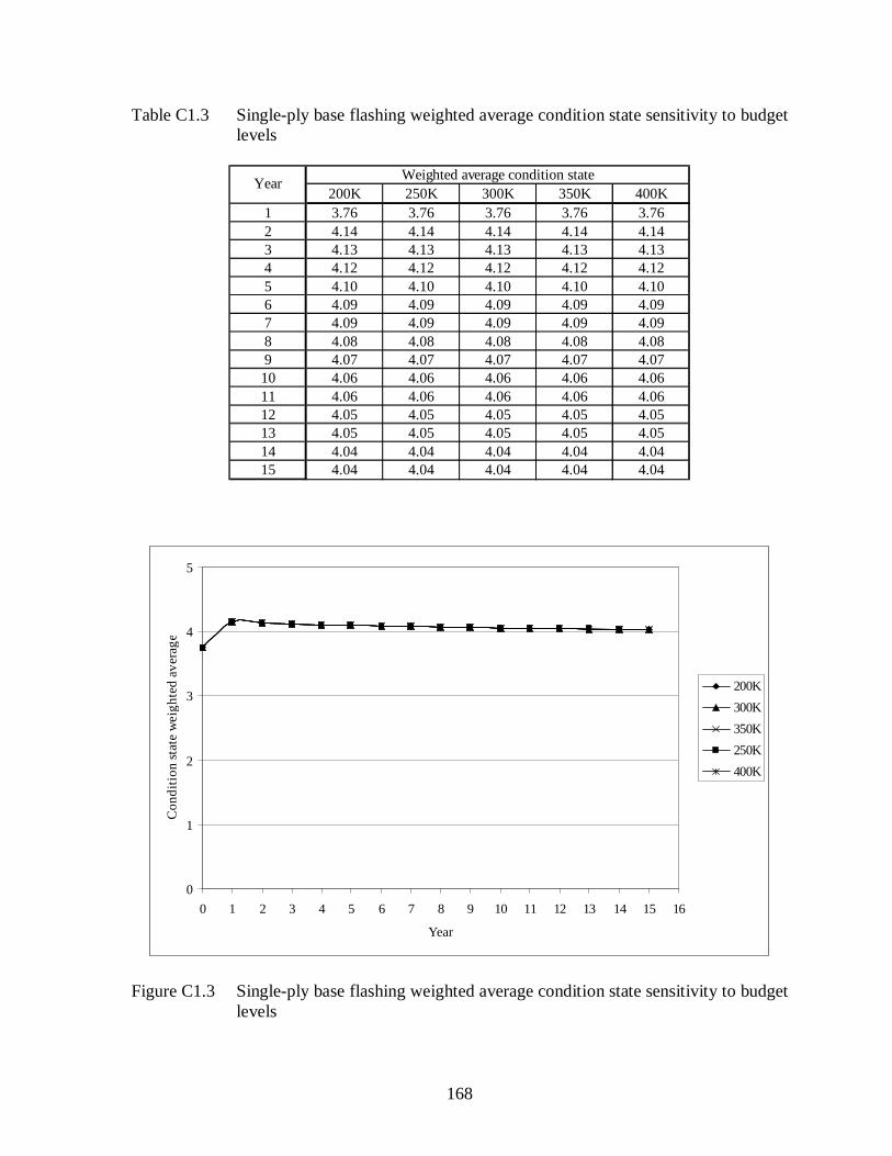
168

Table C1.3 Single-ply base flashing weighted average condition state sensitivity to budget levels

200K 250K 300K 350K 400K1 3.76 3.76 3.76 3.76 3.762 4.14 4.14 4.14 4.14 4.143 4.13 4.13 4.13 4.13 4.134 4.12 4.12 4.12 4.12 4.125 4.10 4.10 4.10 4.10 4.106 4.09 4.09 4.09 4.09 4.097 4.09 4.09 4.09 4.09 4.098 4.08 4.08 4.08 4.08 4.089 4.07 4.07 4.07 4.07 4.0710 4.06 4.06 4.06 4.06 4.0611 4.06 4.06 4.06 4.06 4.0612 4.05 4.05 4.05 4.05 4.0513 4.05 4.05 4.05 4.05 4.0514 4.04 4.04 4.04 4.04 4.0415 4.04 4.04 4.04 4.04 4.04


0

1

2

3

4

5

0 1 2 3 4 5 6 7 8 9 10 11 12 13 14 15 16

Year

Con

ditio

n st

ate

wei

ghte

d av

erag

e

200K300K350K250K400K

Figure C1.3 Single-ply base flashing weighted average condition state sensitivity to budget levels

169

Table C1.4 Multiple-ply base flashing weighted average condition state sensitivity to budget levels

200K 250K 300K 350K 400K1 3.26 3.26 3.26 3.26 3.262 4.23 4.23 4.23 4.23 4.233 4.22 4.22 4.22 4.22 4.224 4.20 4.20 4.20 4.20 4.205 4.18 4.18 4.18 4.18 4.186 4.17 4.17 4.17 4.17 4.177 4.16 4.16 4.16 4.16 4.168 4.14 4.14 4.14 4.14 4.149 4.13 4.13 4.13 4.13 4.1310 4.12 4.12 4.12 4.12 4.1211 4.11 4.11 4.11 4.11 4.1112 4.10 4.10 4.10 4.10 4.1013 4.10 4.10 4.10 4.10 4.1014 4.09 4.09 4.09 4.09 4.0915 4.08 4.08 4.08 4.08 4.08


0

1

2

3

4

5

0 1 2 3 4 5 6 7 8 9 10 11 12 13 14 15 16

Year

Con

ditio

n st

ate

wei

ghte

d av

erag

e

200K250K300K350K400K

Figure C1.4 Multiple-ply base flashing weighted average condition state sensitivity to budget levels

170

Table C1.5 Counter flashing weighted average condition state sensitivity to budget levels

200K 250K 300K 350K 400K1 3.68 3.68 3.68 3.68 3.682 4.15 4.15 4.15 4.15 4.153 4.12 4.12 4.12 4.12 4.124 4.10 4.10 4.10 4.10 4.105 4.09 4.09 4.09 4.09 4.096 4.07 4.07 4.07 4.07 4.077 4.06 4.06 4.06 4.06 4.068 4.05 4.05 4.05 4.05 4.059 4.04 4.04 4.04 4.04 4.0410 4.04 4.04 4.04 4.04 4.0411 4.03 4.03 4.03 4.03 4.0312 4.02 4.02 4.02 4.02 4.0213 4.02 4.02 4.02 4.02 4.0214 4.02 4.02 4.02 4.02 4.0215 4.01 4.01 4.01 4.01 4.01


0

1

2

3

4

5

0 1 2 3 4 5 6 7 8 9 10 11 12 13 14 15 16

Year

Con

ditio

n st

ate

wei

ghte

d av

erag

e

200K250K300K350K400K

Figure C1.5 Counter flashing weighted average condition state sensitivity to budget levels

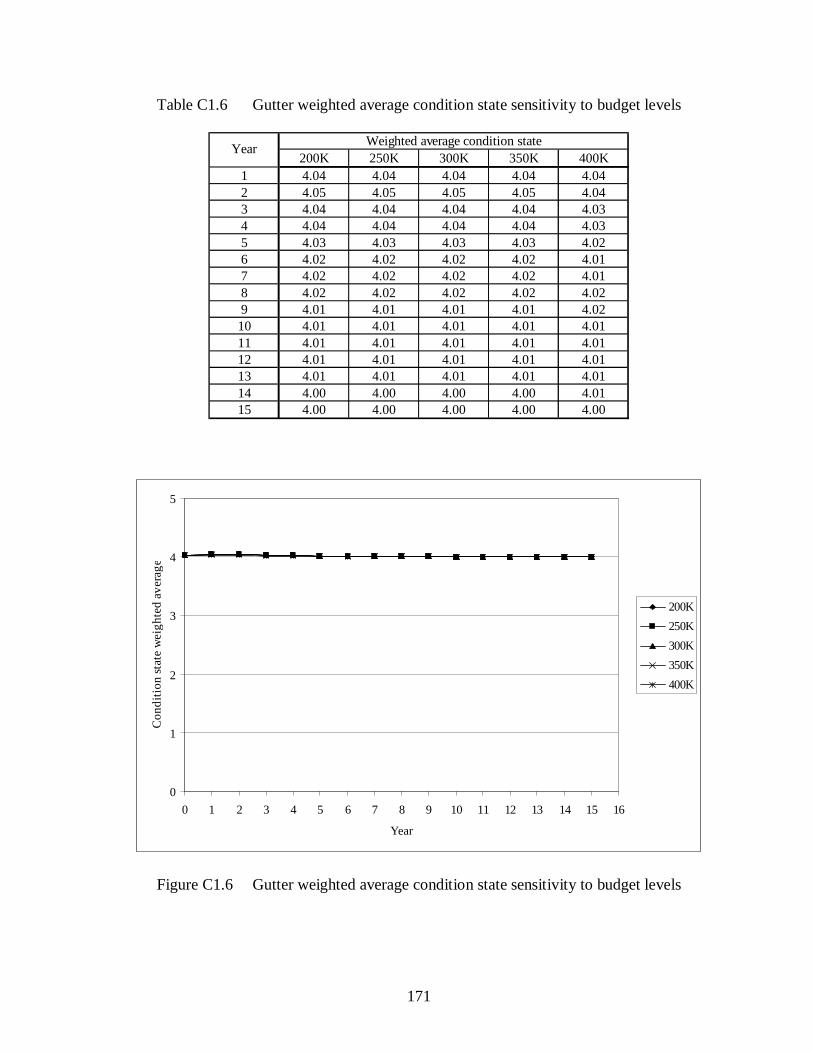
171

Table C1.6 Gutter weighted average condition state sensitivity to budget levels

200K 250K 300K 350K 400K1 4.04 4.04 4.04 4.04 4.042 4.05 4.05 4.05 4.05 4.043 4.04 4.04 4.04 4.04 4.034 4.04 4.04 4.04 4.04 4.035 4.03 4.03 4.03 4.03 4.026 4.02 4.02 4.02 4.02 4.017 4.02 4.02 4.02 4.02 4.018 4.02 4.02 4.02 4.02 4.029 4.01 4.01 4.01 4.01 4.0210 4.01 4.01 4.01 4.01 4.0111 4.01 4.01 4.01 4.01 4.0112 4.01 4.01 4.01 4.01 4.0113 4.01 4.01 4.01 4.01 4.0114 4.00 4.00 4.00 4.00 4.0115 4.00 4.00 4.00 4.00 4.00


0

1

2

3

4

5

0 1 2 3 4 5 6 7 8 9 10 11 12 13 14 15 16

Year

Con

ditio

n st

ate

wei

ghte

d av

erag

e

200K250K300K350K400K

Figure C1.6 Gutter weighted average condition state sensitivity to budget levels

172

Table C1.7 Downspout weighted average condition state sensitivity to budget levels

200K 250K 300K 350K 400K1 4.03 4.03 4.03 4.03 4.032 4.03 4.03 4.03 4.03 4.033 4.03 4.03 4.03 4.03 4.034 4.02 4.02 4.02 4.02 4.025 4.02 4.02 4.02 4.02 4.026 4.01 4.01 4.01 4.01 4.017 4.01 4.01 4.01 4.01 4.018 4.01 4.01 4.01 4.01 4.019 4.01 4.01 4.01 4.01 4.0110 4.01 4.01 4.01 4.01 4.0111 4.01 4.01 4.01 4.01 4.0112 4.00 4.00 4.00 4.00 4.0013 4.00 4.00 4.00 4.00 4.0014 4.00 4.00 4.00 4.00 4.0015 4.00 4.00 4.00 4.00 4.00


0

1

2

3

4

5

0 1 2 3 4 5 6 7 8 9 10 11 12 13 14 15 16

Year

Con

ditio

n st

ate

wei

ghte

d av

erag

e

200K250K300K350K400K

Figure C1.7 Downspout weighted average condition state sensitivity to budget levels

173

Table C1.8 Drain Strainer weighted average condition state sensitivity to budget levels

200K 250K 300K 350K 400K1 3.97 3.97 3.97 3.97 3.972 4.03 4.03 4.03 4.03 4.033 4.02 4.02 4.02 4.02 4.024 4.02 4.02 4.02 4.02 4.025 4.02 4.02 4.02 4.02 4.026 4.01 4.01 4.01 4.01 4.017 4.01 4.01 4.01 4.01 4.018 4.01 4.01 4.01 4.01 4.019 4.01 4.01 4.01 4.01 4.0110 4.01 4.01 4.01 4.01 4.0111 4.01 4.01 4.01 4.01 4.0112 4.01 4.01 4.01 4.01 4.0113 4.01 4.01 4.01 4.01 4.0114 4.00 4.00 4.00 4.00 4.0015 4.00 4.00 4.00 4.00 4.00


0

1

2

3

4

5

0 1 2 3 4 5 6 7 8 9 10 11 12 13 14 15 16

Year

Con

ditio

n st

ate

wei

ghte

d av

erag

e

200K250K300K350K400K

Figure C1.8 Drain Strainer weighted average condition state sensitivity to budget levels

174

Table C1.9 Coping cap weighted average condition state sensitivity to budget levels

200K 250K 300K 350K 400K1 4.02 4.02 4.02 4.02 4.022 4.03 4.03 4.02 4.03 4.033 4.02 4.02 4.01 4.02 4.024 4.02 4.02 4.01 4.02 4.025 4.02 4.02 4.01 4.02 4.026 4.01 4.01 4.00 4.01 4.017 4.01 4.01 4.00 4.01 4.018 4.01 4.01 4.00 4.01 4.019 4.01 4.01 4.00 4.01 4.0110 4.01 4.01 4.00 4.01 4.0111 4.01 4.01 4.00 4.01 4.0112 4.01 4.00 4.00 4.01 4.0113 4.00 4.00 4.00 4.00 4.0014 4.00 3.99 4.01 4.00 4.0015 4.00 4.00 4.01 4.00 4.00


0

1

2

3

4

5

0 1 2 3 4 5 6 7 8 9 10 11 12 13 14 15 16

Year

Con

ditio

n st

ate

wei

ghte

d av

erag

e

250K300K350K400K200K

Figure C1.9 Coping cap weighted average condition state sensitivity to budget levels

175

Table C1.10 Termination bar weighted average condition state sensitivity to budget levels

200K 250K 300K 350K 400K1 4.00 4.00 4.00 4.00 4.002 4.01 4.01 4.01 4.01 4.013 4.01 4.01 4.01 4.01 4.014 4.01 4.01 4.01 4.01 4.015 4.01 4.01 4.01 4.01 4.016 4.00 4.00 4.00 4.00 4.007 4.00 4.00 4.00 4.00 4.008 4.00 4.00 4.00 4.00 4.009 4.00 4.00 4.00 4.00 4.0010 4.00 4.00 4.00 4.00 4.0011 4.00 4.00 4.00 4.00 4.0012 4.00 4.00 4.00 4.00 4.0013 4.00 4.00 4.00 4.00 4.0014 4.00 4.00 4.00 4.00 4.0015 4.00 4.00 4.00 4.00 4.00


0

1

2

3

4

5

0 1 2 3 4 5 6 7 8 9 10 11 12 13 14 15 16

Year

Con

ditio

n st

ate

wei

ghte

d av

erag

e

200K250K300K350K400K

Figure C1.10 Termination bar weighted average condition state sensitivity to budget levels

176

Table C1.11 Edge metal weighted average condition state sensitivity to budget levels

200K 250K 300K 350K 400K1 3.64 3.64 3.64 3.64 3.642 4.15 4.15 4.15 4.15 4.153 4.13 4.13 4.13 4.13 4.134 4.11 4.11 4.11 4.11 4.115 4.10 4.10 4.10 4.10 4.106 4.09 4.09 4.09 4.09 4.097 4.07 4.07 4.07 4.07 4.078 4.07 4.07 4.07 4.07 4.079 4.06 4.06 4.06 4.06 4.0610 4.05 4.05 4.05 4.05 4.0511 4.04 4.04 4.04 4.04 4.0412 4.04 4.04 4.04 4.04 4.0413 4.03 4.03 4.03 4.03 4.0314 4.03 4.03 4.03 4.03 4.0315 4.03 4.03 4.03 4.03 4.03


0

1

2

3

4

5

0 1 2 3 4 5 6 7 8 9 10 11 12 13 14 15 16

Year

Con

ditio

n st

ate

wei

ghte

d av

erag

e

200K250K300K350K400K

Figure C1.11 Edge metal weighted average condition state sensitivity to budget levels

177

Table C1.12 Shingle weighted average condition state sensitivity to budget levels

200K 250K 300K 350K 400K1 4.31 4.31 4.31 4.31 4.312 4.31 4.31 4.31 4.31 4.313 4.29 4.29 4.29 4.29 4.294 4.27 4.27 4.27 4.27 4.275 4.25 4.26 4.26 4.26 4.266 4.25 4.25 4.25 4.25 4.257 4.24 4.25 4.25 4.25 4.248 4.24 4.24 4.23 4.24 4.349 4.23 4.23 4.21 4.23 4.3310 4.23 4.23 4.22 4.23 4.4111 4.23 4.23 4.20 4.23 4.4812 4.22 4.21 4.19 4.33 4.5313 4.21 4.20 4.18 4.41 4.5614 4.20 4.20 4.19 4.48 4.6015 4.20 4.21 4.19 4.53 4.62


0

1

2

3

4

5

0 1 2 3 4 5 6 7 8 9 10 11 12 13 14 15 16

Year

Con

ditio

n st

ate

wei

ghte

d av

erag

e

200K250K300K350K400K

Figure C1.12 Shingle weighted average condition state sensitivity to budget levels

178

Table C1.13 Slate weighted average condition state sensitivity to budget levels

200K 250K 300K 350K 400K1 4.00 4.00 4.00 4.00 4.002 4.00 4.00 4.00 4.00 4.003 4.00 4.00 4.00 4.00 4.004 4.00 4.00 4.00 4.00 4.005 4.00 4.00 4.00 4.00 4.006 4.00 4.00 4.00 4.00 4.007 4.00 4.00 4.00 4.00 4.008 4.00 4.00 4.00 4.00 4.009 4.00 4.00 4.00 4.00 4.0010 4.00 4.00 4.00 4.00 4.0011 4.00 4.00 4.00 4.00 4.0012 4.00 4.00 4.00 4.00 4.0013 4.00 4.00 4.00 4.00 4.0014 4.00 4.00 4.00 4.00 4.0015 4.00 4.00 4.00 4.00 4.00


0

1

2

3

4

5

0 1 2 3 4 5 6 7 8 9 10 11 12 13 14 15 16

Year

Con

ditio

n st

ate

wei

ghte

d av

erag

e

200K250K300K350K400K

Figure C1.13 Slate weighted average condition state sensitivity to budget levels

179

Table C1.14 Hip/ridge cap weighted average condition state sensitivity to budget levels

200K 250K 300K 350K 400K1 4.00 4.00 4.00 4.00 4.002 4.00 4.00 4.00 4.00 4.003 4.00 4.00 4.00 4.00 4.004 4.00 4.00 4.00 4.00 4.005 4.00 4.00 4.00 4.00 4.006 4.00 4.00 4.00 4.00 4.007 4.00 4.00 4.00 4.00 4.008 4.00 4.00 4.00 4.00 4.009 4.00 4.00 4.00 4.00 4.0010 4.00 4.00 4.00 4.00 4.0011 4.00 4.00 4.00 4.00 4.0012 4.00 4.00 4.00 4.00 4.0013 4.00 4.00 4.00 4.00 4.0014 4.00 4.00 4.00 4.00 4.0015 4.00 4.00 4.00 4.00 4.00


0

1

2

3

4

5

0 1 2 3 4 5 6 7 8 9 10 11 12 13 14 15 16

Year

Con

ditio

n st

ate

wei

ghte

d av

erag

e

250K300K350K400K200K

Figure C1.14 Hip/ridge cap weighted average condition state sensitivity to budget levels

180

APPENDIX C2

This appendix includes tables and graphs showing the weighted average condition

state sensitivity to Real Rates of Return of all maintenance elements.

Table C2.1 Single-ply membrane weighted average condition state sensitivity to Real Rate of Return levels

1.50% 3.00% 4.50% 6.00% 7.50%1 3.82 3.82 3.82 3.82 3.822 4.04 4.04 4.04 4.04 4.043 4.00 3.99 3.99 3.99 3.994 4.04 4.03 4.03 4.03 4.035 4.11 4.10 4.10 4.10 4.106 4.19 4.18 4.18 4.18 4.187 4.27 4.26 4.26 4.26 4.268 4.33 4.32 4.32 4.32 4.329 4.39 4.37 4.37 4.37 4.3710 4.42 4.41 4.41 4.41 4.4111 4.44 4.44 4.44 4.44 4.4412 4.46 4.46 4.46 4.46 4.4613 4.46 4.46 4.46 4.48 4.4814 4.50 4.50 4.50 4.50 4.4915 4.62 4.63 4.63 4.62 4.62


0

1

2

3

4

5

0 1 2 3 4 5 6 7 8 9 10 11 12 13 14 15 16

Year

Con

ditio

n st

ate

wei

ghte

d av

erag

e

1.5%3.0%4.5%6.0%7.5%

Figure C2.1 Single-ply membrane weighted average condition state sensitivity to Real

Rate of Return levels

181

Table C2.2 Multiple-ply membrane weighted average condition state sensitivity to Real

Rate of Return levels

1.50% 3.00% 4.50% 6.00% 7.50%1 3.23 3.23 3.23 3.23 3.232 3.23 3.23 3.23 3.23 3.233 3.15 3.16 3.16 3.16 3.164 2.89 2.91 2.91 2.91 2.985 2.72 2.77 2.75 2.75 2.826 2.68 2.72 2.71 2.71 2.787 2.74 2.78 2.78 2.78 2.868 2.92 2.97 2.96 2.97 3.019 3.15 3.21 3.20 3.21 3.2410 3.44 3.48 3.48 3.48 3.5111 3.76 3.79 3.78 3.79 3.8112 4.09 4.12 4.10 4.11 4.1313 4.48 4.50 4.49 4.45 4.5614 4.75 4.75 4.75 4.75 4.7515 4.72 4.72 4.72 4.72 4.72


0

1

2

3

4

5

0 1 2 3 4 5 6 7 8 9 10 11 12 13 14 15 16

Year

Con

ditio

n st

ate

wei

ghte

d av

erag

e

1.5%3.0%4.5%6.0%7.5%

Figure C2.2 Multiple-ply membrane weighted average condition state sensitivity to Real Rate of Return levels

182

Table C2.3 Single-ply base flashing weighted average condition state sensitivity to Real Rate of Return levels

1.50% 3.00% 4.50% 6.00% 7.50%1 3.76 3.76 3.76 3.76 3.762 4.14 4.14 4.14 4.14 4.143 4.13 4.13 4.13 4.13 4.134 4.12 4.12 4.12 4.12 4.125 4.10 4.10 4.10 4.10 4.106 4.09 4.09 4.09 4.09 4.097 4.09 4.09 4.09 4.09 4.098 4.08 4.08 4.08 4.08 4.089 4.07 4.07 4.07 4.07 4.0710 4.06 4.06 4.06 4.06 4.0611 4.06 4.06 4.06 4.06 4.0612 4.05 4.05 4.05 4.05 4.0513 4.05 4.05 4.05 4.05 4.0514 4.04 4.04 4.04 4.04 4.0415 4.04 4.04 4.04 4.04 4.04


0

1

2

3

4

5

0 1 2 3 4 5 6 7 8 9 10 11 12 13 14 15 16

Year

Con

ditio

n st

ate

wei

ghte

d av

erag

e

1.5%3.0%4.5%6.0%7.5%

Figure C2.3 Single-ply base flashing weighted average condition state sensitivity to Real Rate of Return levels

183

Table C2.4 Multiple-ply base flashing weighted average condition state sensitivity to Real Rate of Return levels

1.50% 3.00% 4.50% 6.00% 7.50%1 3.26 3.26 3.26 3.26 3.262 4.23 4.23 4.23 4.23 4.233 4.22 4.22 4.22 4.22 4.224 4.20 4.20 4.20 4.20 4.205 4.18 4.18 4.18 4.18 4.186 4.17 4.17 4.17 4.17 4.177 4.16 4.16 4.16 4.16 4.168 4.14 4.14 4.14 4.14 4.149 4.13 4.13 4.13 4.13 4.1310 4.12 4.12 4.12 4.12 4.1211 4.11 4.11 4.11 4.11 4.1112 4.10 4.10 4.10 4.10 4.1013 4.10 4.10 4.10 4.10 4.1014 4.09 4.09 4.09 4.09 4.0915 4.08 4.08 4.08 4.08 4.08


0

1

2

3

4

5

0 1 2 3 4 5 6 7 8 9 10 11 12 13 14 15 16

Year

Con

ditio

n st

ate

wei

ghte

d av

erag

e

1.5%3.0%4.5%6.0%7.5%

Figure C2.4 Multiple-ply base flashing weighted average condition state sensitivity to Real Rate of Return levels

184

Table C2.5 Counter flashing weighted average condition state sensitivity to Real Rate of Return levels

1.50% 3.00% 4.50% 6.00% 7.50%1 3.68 3.68 3.68 3.68 3.682 4.15 4.15 4.15 4.15 4.153 4.12 4.12 4.12 4.12 4.124 4.10 4.10 4.10 4.10 4.105 4.09 4.09 4.09 4.09 4.096 4.07 4.07 4.07 4.07 4.077 4.06 4.06 4.06 4.06 4.068 4.05 4.05 4.05 4.05 4.059 4.04 4.04 4.04 4.04 4.0410 4.04 4.04 4.04 4.04 4.0411 4.03 4.03 4.03 4.03 4.0312 4.02 4.02 4.02 4.02 4.0213 4.02 4.02 4.02 4.02 4.0214 4.02 4.02 4.02 4.02 4.0215 4.01 4.01 4.01 4.01 4.01


0

1

2

3

4

5

0 1 2 3 4 5 6 7 8 9 10 11 12 13 14 15 16

Year

Con

ditio

n st

ate

wei

ghte

d av

erag

e

1.5%

3.0%4.5%

6.0%

7.5%

Figure C2.5 Counter flashing weighted average condition state sensitivity to Real Rate of Return levels

185

Table C2.6 Gutter weighted average condition state sensitivity to Real Rate of Return levels

1.50% 3.00% 4.50% 6.00% 7.50%1 4.04 4.04 4.04 4.04 4.042 4.04 4.05 4.05 4.04 4.053 4.03 4.04 4.04 4.03 4.044 4.03 4.04 4.04 4.02 4.045 4.03 4.03 4.03 4.02 4.036 4.03 4.02 4.02 4.01 4.027 4.02 4.02 4.02 4.01 4.028 4.02 4.02 4.02 4.00 4.029 4.01 4.01 4.01 4.00 4.0110 4.01 4.01 4.01 4.00 4.0111 4.01 4.01 4.01 4.00 4.0112 4.01 4.01 4.01 3.99 4.0113 4.01 4.01 4.01 3.99 4.0114 4.01 4.00 4.00 4.01 4.0015 4.00 4.00 4.00 4.01 4.00


0

1

2

3

4

5

0 1 2 3 4 5 6 7 8 9 10 11 12 13 14 15 16

Year

Con

ditio

n st

ate

wei

ghte

d av

erag

e

1.5%3.0%

4.5%6.0%

7.5%

Figure C2.6 Gutter weighted average condition state sensitivity to Real Rate of Return levels

186

Table C2.7 Downspout weighted average condition state sensitivity to Real Rate of Return levels

1.50% 3.00% 4.50% 6.00% 7.50%1 4.03 4.03 4.03 4.03 4.032 4.03 4.03 4.03 4.03 4.033 4.03 4.03 4.03 4.03 4.034 4.02 4.02 4.02 4.02 4.025 4.02 4.02 4.02 4.02 4.026 4.01 4.01 4.01 4.01 4.017 4.01 4.01 4.01 4.01 4.018 4.01 4.01 4.01 4.01 4.019 4.01 4.01 4.01 4.01 4.0110 4.01 4.01 4.01 4.01 4.0111 4.01 4.01 4.01 4.01 4.0112 4.00 4.00 4.00 4.00 4.0013 4.00 4.00 4.00 4.00 4.0014 4.00 4.00 4.00 4.00 4.0015 4.00 4.00 4.00 4.00 4.00


0

1

2

3

4

5

0 1 2 3 4 5 6 7 8 9 10 11 12 13 14 15 16

Year

Con

ditio

n st

ate

wei

ghte

d av

erag

e

1.5%3.0%

4.5%6.0%7.5%

Figure C2.7 Downspout weighted average condition state sensitivity to Real Rate of Return levels

187

Table C2.8 Drain Strainer weighted average condition state sensitivity to Real Rate of Return levels

1.50% 3.00% 4.50% 6.00% 7.50%1 3.97 3.97 3.97 3.97 3.972 4.03 4.03 4.03 4.03 4.033 4.02 4.02 4.02 4.02 4.024 4.02 4.02 4.02 4.02 4.025 4.02 4.02 4.02 4.02 4.026 4.01 4.01 4.01 4.01 4.017 4.01 4.01 4.01 4.01 4.018 4.01 4.01 4.01 4.01 4.019 4.01 4.01 4.01 4.01 4.0110 4.01 4.01 4.01 4.01 4.0111 4.01 4.01 4.01 4.01 4.0112 4.01 4.01 4.01 4.01 4.0113 4.01 4.01 4.01 4.01 4.0114 4.00 4.00 4.00 4.00 4.0015 4.00 4.00 4.00 4.00 4.00


0

1

2

3

4

5

0 1 2 3 4 5 6 7 8 9 10 11 12 13 14 15 16

Year

Con

ditio

n st

ate

wei

ghte

d av

erag

e

1.5%

3.0%4.5%6.0%

7.5%

Figure C2.8 Drain Strainer weighted average condition state sensitivity to Real Rate of Return levels

188

Table C2.9 Coping cap weighted average condition state sensitivity to Real Rate of Return levels

1.50% 3.00% 4.50% 6.00% 7.50%1 4.02 4.02 4.02 4.02 4.022 4.03 4.02 4.03 4.03 4.033 4.02 4.01 4.02 4.02 4.024 4.02 4.01 4.02 4.02 4.025 4.02 4.01 4.02 4.02 4.026 4.01 4.00 4.01 4.01 4.017 4.01 4.00 4.01 4.01 4.018 4.01 4.00 4.01 4.01 4.019 4.01 4.00 4.01 4.01 4.0110 4.01 4.00 4.01 4.01 4.0111 4.01 4.00 4.01 4.01 4.0112 4.01 4.00 4.01 4.01 4.0113 4.00 4.00 4.00 4.00 3.8514 4.00 4.01 4.00 4.00 4.0515 4.00 4.01 4.00 4.00 4.05


0

1

2

3

4

5

0 1 2 3 4 5 6 7 8 9 10 11 12 13 14 15 16

Year

Cond

ition

stat

e w

eigh

ted

aver

age

1.5%3.0%4.5%6.0%7.5%

Figure C2.9 Coping cap weighted average condition state sensitivity to Real Rate of Return levels

189

Table C2.10 Termination bar weighted average condition state sensitivity to Real Rate of Return levels

1.50% 3.00% 4.50% 6.00% 7.50%1 4.00 4.00 4.00 4.00 4.002 4.01 4.01 4.01 4.01 4.013 4.01 4.01 4.01 4.01 4.014 4.01 4.01 4.01 4.01 4.015 4.01 4.01 4.01 4.01 4.016 4.00 4.00 4.00 4.00 4.007 4.00 4.00 4.00 4.00 4.008 4.00 4.00 4.00 4.00 4.009 4.00 4.00 4.00 4.00 4.0010 4.00 4.00 4.00 4.00 4.0011 4.00 4.00 4.00 4.00 4.0012 4.00 4.00 4.00 4.00 4.0013 4.00 4.00 4.00 4.00 4.0014 4.00 4.00 4.00 4.00 4.0015 4.00 4.00 4.00 4.00 4.00


0

1

2

3

4

5

0 1 2 3 4 5 6 7 8 9 10 11 12 13 14 15 16

Year

Cond

ition

stat

e w

eigh

ted

aver

age

1.5%3.0%4.5%6.0%7.5%

Figure C2.10 Termination bar weighted average condition state sensitivity to Real Rate of Return levels

190

Table C2.11 Edge metal weighted average condition state sensitivity to Real Rate of Return levels

1.50% 3.00% 4.50% 6.00% 7.50%1 3.64 3.64 3.64 3.64 3.642 4.15 4.15 4.15 4.15 4.153 4.13 4.13 4.13 4.13 4.134 4.11 4.11 4.11 4.11 4.115 4.10 4.10 4.10 4.10 4.106 4.09 4.09 4.09 4.09 4.097 4.07 4.07 4.07 4.07 4.078 4.07 4.07 4.07 4.07 4.079 4.06 4.06 4.06 4.06 4.0610 4.05 4.05 4.05 4.05 4.0511 4.04 4.04 4.04 4.04 4.0412 4.04 4.04 4.04 4.04 4.0413 4.03 4.03 4.03 4.03 4.0314 4.03 4.03 4.03 4.03 4.0315 4.03 4.03 4.03 4.03 4.03


0

1

2

3

4

5

0 1 2 3 4 5 6 7 8 9 10 11 12 13 14 15 16

Year

Cond

ition

stat

e w

eigh

ted

aver

age

1.5%3.0%4.5%6.0%7.5%

Figure C2.11 Edge metal weighted average condition state sensitivity to Real Rate of Return levels

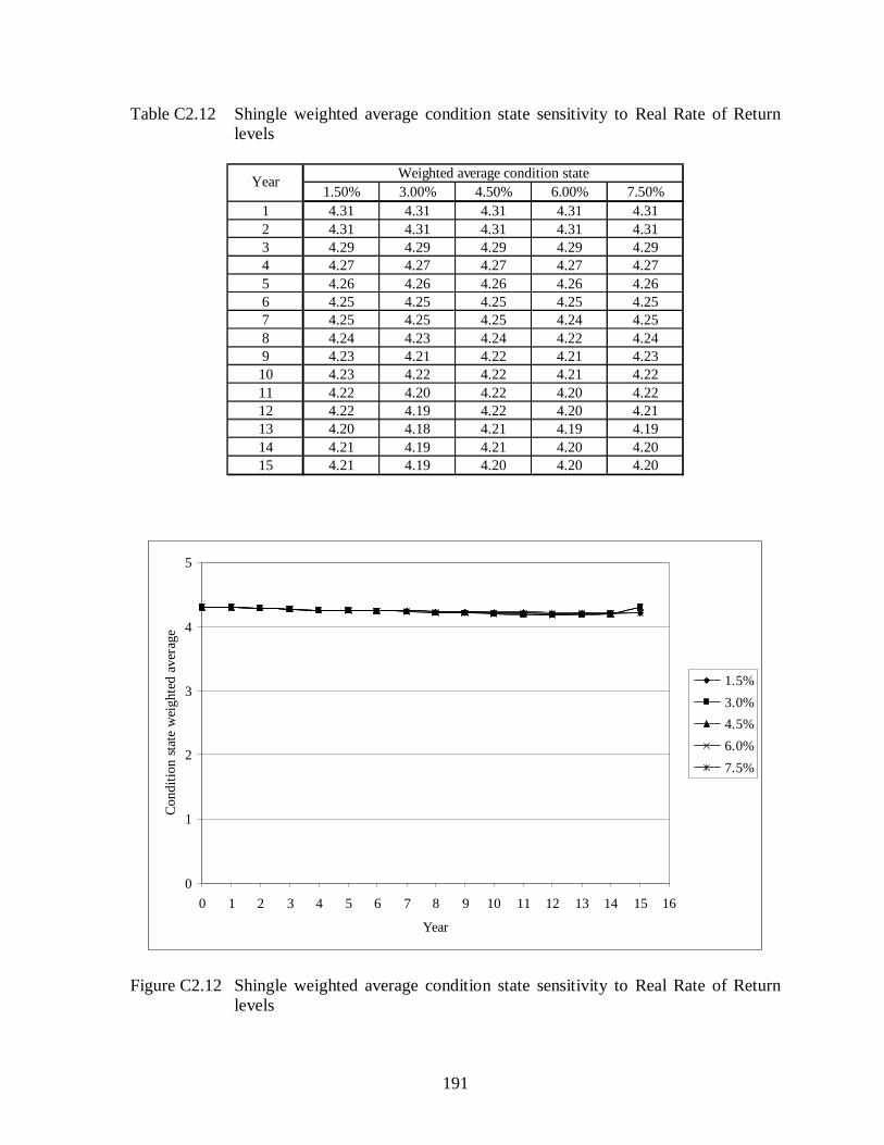
191

Table C2.12 Shingle weighted average condition state sensitivity to Real Rate of Return levels

1.50% 3.00% 4.50% 6.00% 7.50%1 4.31 4.31 4.31 4.31 4.312 4.31 4.31 4.31 4.31 4.313 4.29 4.29 4.29 4.29 4.294 4.27 4.27 4.27 4.27 4.275 4.26 4.26 4.26 4.26 4.266 4.25 4.25 4.25 4.25 4.257 4.25 4.25 4.25 4.24 4.258 4.24 4.23 4.24 4.22 4.249 4.23 4.21 4.22 4.21 4.2310 4.23 4.22 4.22 4.21 4.2211 4.22 4.20 4.22 4.20 4.2212 4.22 4.19 4.22 4.20 4.2113 4.20 4.18 4.21 4.19 4.1914 4.21 4.19 4.21 4.20 4.2015 4.21 4.19 4.20 4.20 4.20


0

1

2

3

4

5

0 1 2 3 4 5 6 7 8 9 10 11 12 13 14 15 16

Year

Cond

ition

stat

e w

eigh

ted

aver

age

1.5%3.0%4.5%6.0%7.5%

Figure C2.12 Shingle weighted average condition state sensitivity to Real Rate of Return levels

192

Table C2.13 Slate weighted average condition state sensitivity to Real Rate of Return levels

1.50% 3.00% 4.50% 6.00% 7.50%1 4.00 4.00 4.00 4.00 4.002 4.00 4.00 4.00 4.00 4.003 4.00 4.00 4.00 4.00 4.004 4.00 4.00 4.00 4.00 4.005 4.00 4.00 4.00 4.00 4.006 4.00 4.00 4.00 4.00 4.007 4.00 4.00 4.00 4.00 4.008 4.00 4.00 4.00 4.00 4.009 4.00 4.00 4.00 4.00 4.0010 4.00 4.00 4.00 4.00 4.0011 4.00 4.00 4.00 4.00 4.0012 4.00 4.00 4.00 4.00 4.0013 4.00 4.00 4.00 4.00 3.9614 4.00 4.00 4.00 4.00 3.9915 4.00 4.00 4.00 4.00 4.00


0

1

2

3

4

5

0 1 2 3 4 5 6 7 8 9 10 11 12 13 14 15 16

Year

Cond

ition

stat

e w

eigh

ted

aver

age

1.5%3.0%4.5%6.0%7.5%

Figure C2.13 Slate weighted average condition state sensitivity to Real Rate of Return levels

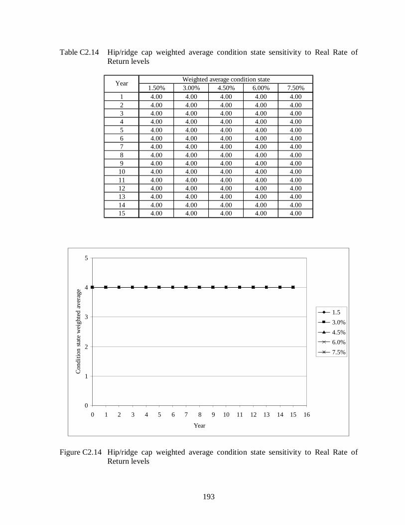
193

Table C2.14 Hip/ridge cap weighted average condition state sensitivity to Real Rate of Return levels

1.50% 3.00% 4.50% 6.00% 7.50%1 4.00 4.00 4.00 4.00 4.002 4.00 4.00 4.00 4.00 4.003 4.00 4.00 4.00 4.00 4.004 4.00 4.00 4.00 4.00 4.005 4.00 4.00 4.00 4.00 4.006 4.00 4.00 4.00 4.00 4.007 4.00 4.00 4.00 4.00 4.008 4.00 4.00 4.00 4.00 4.009 4.00 4.00 4.00 4.00 4.0010 4.00 4.00 4.00 4.00 4.0011 4.00 4.00 4.00 4.00 4.0012 4.00 4.00 4.00 4.00 4.0013 4.00 4.00 4.00 4.00 4.0014 4.00 4.00 4.00 4.00 4.0015 4.00 4.00 4.00 4.00 4.00


0

1

2

3

4

5

0 1 2 3 4 5 6 7 8 9 10 11 12 13 14 15 16

Year

Cond

ition

stat

e w

eigh

ted

aver

age

1.53.0%4.5%6.0%7.5%

Figure C2.14 Hip/ridge cap weighted average condition state sensitivity to Real Rate of Return levels

Documents

Optimizing Roof Maintenance and Replacement Decisions