Optimizing shrub parameters to estimate gross … based models like LPJ -DGVM (Lund -Potsman -Jena Dynamic Vegetation Model) (S itch et al., 2003) , and B IOME BGC (Running and Hunt,

1

Optimizing shrub parameters to estimate gross primary production

of the sagebrush ecosystem using the Ecosystem Demography

(EDv2.2) model

Karun Pandit1, Hamid Dashti1, Nancy F. Glenn1, Alejandro N. Flores1, Kaitlin C. Maguire2, Douglas J.

Shinneman2, Gerald N. Flerchinger3, Aaron W. Fellows3 5

1Department of Geosciences, Boise State University, 1910 University Dr., Boise, ID 83725-1535 USA 2United States Geological Survey, Forest and Rangeland Ecosystem Science Center, 970 Lusk St., Boise, ID 83706 3United States Department of Agriculture, Agricultural Research Service, 800 Park Blvd., Suite 105, Boise, ID 83712

Correspondence to: Karun Pandit ([email protected])

Abstract. Gross primary production (GPP) is one of the most critical processes in the global carbon cycle, but is difficult to 10

quantify in part because of its high spatiotemporal variability. Direct techniques to quantify GPP are lacking, thus, researchers

rely on data inferred from eddy covariance (EC) towers and/or ecosystem dynamic models. The latter are useful to quantify

GPP over time and space because of their efficiency over direct field measurements and applicability to broad spatial extents.

However, such models have also been associated with internal uncertainties and complexities arising from distinct qualities of

the ecosystem being analyzed. Widely distributed sagebrush-steppe ecosystems in western North America are threatened by 15

anthropogenic disturbance, invasive species, climate change, and altered fire regimes. Although land managers have focused

on different restoration techniques, the effects of these activities and their interactions with fire, climate change, and invasive

species on ecosystem dynamics are poorly understood. In this study, we applied an ecosystem dynamic model, Ecosystem

Demography (EDv2.2), to parameterize and predict GPP for sagebrush-steppe ecosystems in the Reynolds Creek Experimental

Watershed (RCEW), located in the northern Great Basin. Our primary objective was to develop and parameterize a sagebrush 20

(Artemisia spp.) shrubland Plant Functional Type (PFT) for use in the EDv2.2 model, which will support future studies to

model estimates of GPP under different climate and management scenarios. To accomplish this, we employed a three-tiered

approach. First, to parameterize the sagebrush PFT, we fitted allometric relationships for sagebrush using field-collected data,

gathered information from existing sagebrush literature, and borrowed values from other PFTs in EDv2.2. Second, we

identified the five most sensitive parameters out of eleven that were found to be influential in GPP prediction based on previous 25

studies. Third, we optimized the five parameters using an exhaustive search method to predict GPP, and performed validation

using observations from two EC sites in the study area. Our modeled results were encouraging, with reasonable fidelity to

observed values, although some negative biases (i.e., seasonal underestimates of GPP) were apparent. We expect that, with

further refinement, the resulting sagebrush PFT will permit explicit scenario testing of potential anthropogenic modifications

of GPP in sagebrush ecosystems, and will contribute to a better understanding of the role of sagebrush ecosystems in shaping 30

global carbon cycles.

Geosci. Model Dev. Discuss., https://doi.org/10.5194/gmd-2018-264Manuscript under review for journal Geosci. Model Dev.Discussion started: 13 December 2018c© Author(s) 2018. CC BY 4.0 License.

2

1 Introduction

Terrestrial gross primary production (GPP) is a major driver of the global carbon cycle as it plays an important role in regulation

of atmospheric CO2 by offsetting anthropogenic CO2 emissions. GPP quantifies the rate of carbon uptake from the atmosphere

through photosynthesis and is often presented as one of the most critical elements in global carbon research because of its high

spatiotemporal variability (Chen, 2012; Zhao and Running, 2010). Since direct techniques to quantify GPP are lacking, 5

researchers derive estimates using observations from eddy covariance (EC) towers or using ecosystem dynamic models (Dong

et al., 2017; Turner et al., 2006; Zhao et al., 2005). Ecosystem models have been widely used to estimate terrestrial carbon

flux and to project ecosystem dynamics over time and space (Dietze et al., 2014; Fisher et al., 2017), largely due to their

efficiency over direct field measurements and their applicability to broader spatial scales. However, these models have also

been associated with high levels of uncertainty and complexity associated with their applicability to distinct ecosystems. 10

Mainly, three different types of errors have been associated with these models: (1) process error arising from formulations in

the model and associated parameters, (2) forcing error related to the quality of meteorological data, and (3) the initial ecosystem

state at the start of the simulation (Antonarakis et al., 2014; Huntzinger et al., 2012). Initialization error is generally not an

issue for long-term simulations, and researchers can minimize both forcing and initialization errors by using observational data

rather than reanalysis data (Antonorakis et al., 2014; Medvigy et al., 2009). Indeed, process error is the most problematic, as 15

it can mask uncertainties caused by forcing errors and can create potential bias in predictions. Fortunately, process error can

be quantified and minimized by systematically comparing model predictions with observable ecosystem metrics (Braswell et

al., 2005; Dietze et al., 2014; Medvigy et al., 2009).

Another critical limitation to widely applying ecosystem dynamic models is their suitability for a unique ecosystem for

which they have not been parametrized. Semi-arid, non-forest ecosystems provide an excellent example of this limitation, 20

including sagebrush (Artemisia spp.) ecosystems, one of the most widespread community types in North America. Sagebrush

ecosystems hold high ecological and social value, but have been reduced to nearly half of their historical range and are

declining at an alarming rate (Knick et al., 2003; Schroeder et al., 2004). Various factors have contributed to this decline,

including land clearing, invasion of nonnative species such as cheatgrass (Bromus tectorum), and climate change, that have

collectively altered vegetation composition, hydrological function, and wildfire frequency (Bradley, 2010; Connelly et al., 25

2004; McArthur and Plummer, 1978; Schlaepfer et al., 2014). In order to restore the sagebrush ecosystem, land managers have

focused on suppressing fire, reducing flammable vegetation, controlling invasive species, and seeding native species

(Chambers et al., 2014; McIver and Brunson, 2014). There are relatively few studies that have evaluated carbon flux in

sagebrush ecosystems in response to prescribed fire or restoration activities, and most of them used observational data from

EC stations. Previous studies identified temporal variation in net carbon exchange rates after restoration treatments, including 30

documenting increases in carbon uptake in the early years after prescribed fire (caused by re-sprouting shrubs and fast growing

grasses), followed by an eventual levelling off to pre-fire conditions (Cleary et al., 2010; Fellows et al., 2018). However,

because of the paucity in EC station sites, coupled with the large spatial extent of the sagebrush ecosystems in the Great Basin,


3

the collective effects of restoration activities, fire, climate change, and invasive species on the spatiotemporal dynamics of

structure, composition, and function of ecosystem are poorly understood.

In this study, we applied an ecosystem dynamic model, Ecosystem Demography (EDv2.2) (Medvigy et al., 2009; Moorcroft

et al., 2001), to parameterize and predict GPP for sagebrush ecosystems in an experimental watershed located in the northern

Great Basin. The Great Basin is a ~500,000 km2 cold-desert region dominated by expansive, shrub-steppe ecosystems. Our 5

primary objective was to develop preliminary sagebrush Plant Functional Type (PFT) parameters in the EDv2.2 model, based

on sensitivity analysis and optimization, with respect to GPP prediction. EDv2.2 was originally developed for tropical forest

ecosystems (Moorcroft et al., 2001), and it has been tested in boreal forests (Trugman et al., 2016), temperate forests

(Antonarakis et al., 2014; Medvigy et al., 2009; Medvigy et al., 2013), and tundra (Davidson et al., 2011), however, its

application to semi-arid shrubland ecosystems has not been explored. Preliminary parameterization of sagebrush PFT, from 10

this study, will be a first step towards further studies on shrubland ecosystem using EDv2.2 or any other terrestrial models.

2 Materials and methods

2.1 Ecosystem Demography (EDv2.2) model

The Ecosystem Demography (EDv2.2) is a process-based terrestrial biosphere model, which occupies a mid-point on the

continuum of models from individual-based (or gap) models to area-based (or big-leaf) models (Fisher, 2010; Smith et al., 15

2001). Area based models like LPJ-DGVM (Lund-Potsman-Jena Dynamic Vegetation Model) (Sitch et al., 2003), and BIOME

BGC (Running and Hunt, 1993 as cited in Bond-Lamberty et al., 2014) represent plant communities with area-averaged

representation of a plant function type (PFT) for each grid cell. The simplification and computational efficiency of these models

make them widely applicable for regional ecosystem analysis, however, this advantage comes in trade-off with their failure to

capture light competition, competitive exclusion, and disturbances (Fisher, 2010; Bond-Lamberty et al., 2014; Smith et al, 20

2001). On the other hand, individual-based models such as JABOWA (Botkin et al., 1972), and SORTIE (Pacala et al., 1993)

represent vegetation at individual plant level thus making it possible to incorporate competition, coexistence, and disturbances.

The disadvantage of IBMs is that they are often confined to limited spatial and temporal scales due to added computational

burden. EDv2.2 is a cohort based model where individual plants with similar properties, in terms of size, age, and function,

are grouped together to reduce the computational cost while retaining most of the dynamics of IBMs. Each cohort is defined 25

by a PFT, number of plants per unit area, and dimensions of a single representative plant like diameter, height, structural

biomass, and live biomass (Fisher et al., 2010).

In EDv2.2, land surface is composed of a series of gridded cells, which experience meteorological forcing from a

corresponding gridded data or from a coupled atmospheric model (Medvigy, 2006). The mechanistic scaling from individual

to the region is achieved through size and age structured partial differential equations that closely approximate mean behaviour 30

of stochastic gap model (Medvigy et al., 2009; Moorcroft et al., 2001). Each grid cell is subdivided into a series of dynamic

horizontal tiles, which represent locations that had experienced similar disturbance history and has an explicit vertical canopy


4

structure. This mechanism helps capture both vertical and horizontal distribution of vegetation structure and compositional

heterogeneity compared to area-based models (Kim et al., 2012; Moorcroft et al., 2001; Moorcroft et al., 2003; Sellers et al.,

1992). EDv2.2 consists of multiple sub-models for plant growth and mortality, phenology, disturbance, biodiversity,

hydrology, land surface biophysics, and soil biogeochemistry, to predict short-term and long-term ecosystem flux and to

represent natural and anthropogenic disturbances (Kim et al., 2012; Medvigy et al., 2009; Zhang et al., 2015). Sub-models in 5

EDv2.2 rely mostly on many PFT-specific parameters, representing unique attributes of that particular group of species, to

resolve the stated biological processes (Knox et al., 2015). EDv2.2 has parameters defined for 17 different PFTs including

grasses (C3 & C4), conifers, and deciduous trees (temperate & tropical), and agricultural crops. In this study, we identified

parameters for sagebrush (shrub) ecosystem to simulate it in the model as a new PFT. Furthermore, since we focussed on GPP

prediction, we selected eleven different parameters related to plant ecophysiology and biomass allocation from overall to 10

conduct sensitivity and optimization study. We used similar studies (Dietze et al., 2014; Fisher et al., 2010; LeBauer et al.,

2013; Medvigy et al., 2009; Mo et al., 2008; Pereira et al., 2017), preliminary sensitivity analyses, and consultation with other

developers and users of the EDv2.2 model to select these parameters. These included maximum photosynthetic capacity at

15⁰ C (Vm0), specific leaf area (SLA), fine root turnover rate, leaf turnover rate, storage turnover rate, slope of stomatal

conductance-photosynthesis relationship (stomatal slope), ratio of fine roots to leaves (Q), water conductance, cuticular 15

conductance, growth respiration factor (GRF), and leaf width.

As we can find detailed descriptions of sub-models of EDv2.2 in the existing literature (Medvigy et al., 2009; Moorcroft

et al., 2001), here we are trying to describe the ones related to the parameters we have used in this study. The ecophysiological

sub-model has a coupled photosynthesis and stomatal conductance scheme developed by Farquhar and Sharkey (1982) and 20

Leuning (1995) respectively takes care of leaf-level carbon and water fluxes. Leaf-level carbon demand of C3 plants is

determined by the minimum of light-limited rate (Je) and Rubisco-limited rate (Jc), and Vm0 controls the later as given by Eq.(1)

after being scaled to a given temperature.

𝐽𝑐 =𝑉𝑚(𝑇𝑣)(𝐶𝑖𝑛𝑡𝑒𝑟− Г)

𝐶𝑖𝑛𝑡𝑒𝑟+ 𝐾1(1+𝐾2) (1)

25

where, 𝑉𝑚(𝑇𝑣) is the maximum capacity of Rubisco to perform carboxylase function at a given temperature Tv scaled from

Vm0, 𝐶𝑖𝑛𝑡𝑒𝑟is the intercellular CO2 concentration, Г is the compensation point for gross photosynthesis, K1 is the Michaelis-

Menten coefficient for CO2, and K2 is proportional to the Michaelis-Menten coefficient for O2. Stomatal conductance which

is modeled using Leuning (1995), a variant of Ball Berry model (Eq. 2), is influenced by stomatal slope and cuticular

conductance. 30

𝑔𝑠𝑤

=𝑀𝐴𝑜

(𝐶𝑠−Г) (1+𝐷𝑠𝐷0

)+ 𝑏 (2)


5

where, 𝐴𝑜 is photosynthetic rate, 𝑔𝑠𝑤

is stomatal conductance for water, 𝑀 is stomatal slope, 𝑏 is cuticular conductance, 𝐷0 is

empirical constant, 𝐷𝑠 is water vapour deficit and CO2 concentration within leaf boundary, and Г is as described above.

Stomatal control is also affected by soil moisture supply term, which is a function of soil moisture, fine root biomass, and

water conductance. Water and CO2 concentrations within the leaf boundary layer is influenced by leaf width along with other

factors like wind speed, leaf area index, and molecular diffusivity of heat. Specific leaf area (SLA) has units of leaf are per 5

unit leaf carbon and is used scale up leaf-level fluxes to canopy-level fluxes. Relationship between growth respiration and net

photosynthesis is controlled by the growth respiration factor. In EDv2.2, while leaf biomass is determined by allometric

equations based on diameter, fine root biomass is defined by a ratio of leaves to fine roots. Leaf turnover and fine root turnover

rates together influence overall litter turnover rate, even though in deciduous trees dropping of leaves also affects this rate.

Turnover rate of stored leaf pool and storage respiration depends on storage turnover rate, size of stored leaf pool, and storage 10

biomass.

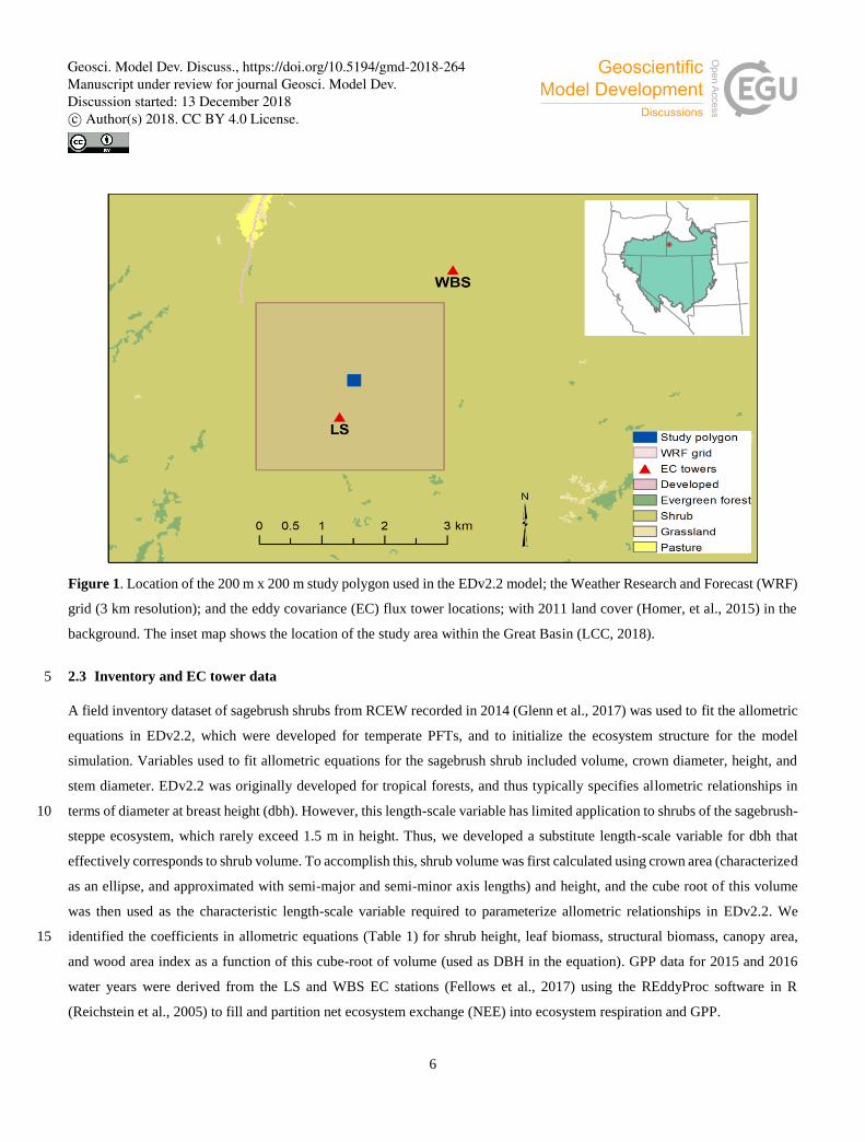
2.2 Study area

We initialized and performed parameter optimization for sagebrush ecosystems in the EDv2.2 model using field data and two

EC station sites located in the Reynolds Creek Experimental Watershed (RCEW) and Critical Zone Observatory (CZO), 15

operated by the USDA Agricultural Research Service (Fig. 1). We used a 200 m x 200 m polygon with center location of 43.15

N and 116.72 W and a mean elevation of 1583 m. The AmeriFlux US-Rls EC station, located at 43.1439 N and 116.7356 W

within the Lower Sheep Creek drainage is approximately 0.7 km from the center of our study site. The area within the footprint

of this tower is dominated by low sagebrush (Artemisia arbuscula) and Sandberg bluegrass (Poa secunda) (Stephenson, 1970;

Seyfried et al., 2000) and is characterized as having light cattle grazing (AmeriFlux, 2018). Another AmeriFlux tower, US-20

Rws, is located at 43.1675 N and 116.7132 W in the Nancy Gulch drainage, within about 2.5 km distance to the northeast from

the study polygon. This area is dominated by Wyoming big sagebrush (A. tridentata ssp. wyomingensis) and bluebunch

wheatgrass (Pseudoroegneria spicata) (Stephenson, 1970). Hereafter, these two sites are designated as LS (for low sagebrush)

and WBS (for Wyoming big sagebrush), respectively.

25


6

Figure 1. Location of the 200 m x 200 m study polygon used in the EDv2.2 model; the Weather Research and Forecast (WRF)

grid (3 km resolution); and the eddy covariance (EC) flux tower locations; with 2011 land cover (Homer, et al., 2015) in the

background. The inset map shows the location of the study area within the Great Basin (LCC, 2018).

2.3 Inventory and EC tower data 5

A field inventory dataset of sagebrush shrubs from RCEW recorded in 2014 (Glenn et al., 2017) was used to fit the allometric

equations in EDv2.2, which were developed for temperate PFTs, and to initialize the ecosystem structure for the model

simulation. Variables used to fit allometric equations for the sagebrush shrub included volume, crown diameter, height, and

stem diameter. EDv2.2 was originally developed for tropical forests, and thus typically specifies allometric relationships in

terms of diameter at breast height (dbh). However, this length-scale variable has limited application to shrubs of the sagebrush-10

steppe ecosystem, which rarely exceed 1.5 m in height. Thus, we developed a substitute length-scale variable for dbh that

effectively corresponds to shrub volume. To accomplish this, shrub volume was first calculated using crown area (characterized

as an ellipse, and approximated with semi-major and semi-minor axis lengths) and height, and the cube root of this volume

was then used as the characteristic length-scale variable required to parameterize allometric relationships in EDv2.2. We

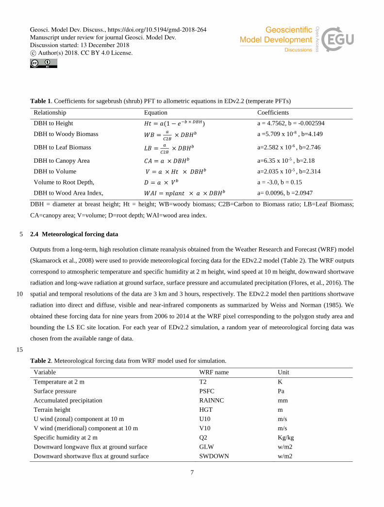
identified the coefficients in allometric equations (Table 1) for shrub height, leaf biomass, structural biomass, canopy area, 15

and wood area index as a function of this cube-root of volume (used as DBH in the equation). GPP data for 2015 and 2016

water years were derived from the LS and WBS EC stations (Fellows et al., 2017) using the REddyProc software in R

(Reichstein et al., 2005) to fill and partition net ecosystem exchange (NEE) into ecosystem respiration and GPP.


7

Table 1. Coefficients for sagebrush (shrub) PFT to allometric equations in EDv2.2 (temperate PFTs)

Relationship Equation Coefficients

DBH to Height 𝐻𝑡 = 𝑎(1 − 𝑒−𝑏 × 𝐷𝐵𝐻) a = 4.7562, b = -0.002594

DBH to Woody Biomass 𝑊𝐵 =𝑎

𝐶2𝐵 × 𝐷𝐵𝐻𝑏 a =5.709 x 10-8 , b=4.149

DBH to Leaf Biomass 𝐿𝐵 =𝑎

𝐶2𝐵 × 𝐷𝐵𝐻𝑏 a=2.582 x 10-6 , b=2.746

DBH to Canopy Area 𝐶𝐴 = 𝑎 × 𝐷𝐵𝐻𝑏 a=6.35 x 10-5 , b=2.18

DBH to Volume 𝑉 = 𝑎 × 𝐻𝑡 × 𝐷𝐵𝐻𝑏 a=2.035 x 10-5 , b=2.314

Volume to Root Depth, 𝐷 = 𝑎 × 𝑉𝑏 a = -3.0, b = 0.15

DBH to Wood Area Index, 𝑊𝐴𝐼 = 𝑛𝑝𝑙𝑎𝑛𝑡 × 𝑎 × 𝐷𝐵𝐻𝑏 a= 0.0096, b =2.0947

DBH = diameter at breast height; Ht = height; WB=woody biomass; C2B=Carbon to Biomass ratio; LB=Leaf Biomass;

CA=canopy area; V=volume; D=root depth; WAI=wood area index.

2.4 Meteorological forcing data 5

Outputs from a long-term, high resolution climate reanalysis obtained from the Weather Research and Forecast (WRF) model

(Skamarock et al., 2008) were used to provide meteorological forcing data for the EDv2.2 model (Table 2). The WRF outputs

correspond to atmospheric temperature and specific humidity at 2 m height, wind speed at 10 m height, downward shortwave

radiation and long-wave radiation at ground surface, surface pressure and accumulated precipitation (Flores, et al., 2016). The

spatial and temporal resolutions of the data are 3 km and 3 hours, respectively. The EDv2.2 model then partitions shortwave 10

radiation into direct and diffuse, visible and near-infrared components as summarized by Weiss and Norman (1985). We

obtained these forcing data for nine years from 2006 to 2014 at the WRF pixel corresponding to the polygon study area and

bounding the LS EC site location. For each year of EDv2.2 simulation, a random year of meteorological forcing data was

chosen from the available range of data.

15

Table 2. Meteorological forcing data from WRF model used for simulation.

Variable WRF name Unit

Temperature at 2 m T2 K

Surface pressure PSFC Pa

Accumulated precipitation RAINNC mm

Terrain height HGT m

U wind (zonal) component at 10 m U10 m/s

V wind (meridional) component at 10 m V10 m/s

Specific humidity at 2 m Q2 Kg/kg

Downward longwave flux at ground surface GLW w/m2

Downward shortwave flux at ground surface SWDOWN w/m2


8

2.5 Initial parameterization and sensitivity analysis

We identified initial shrub PFT parameters based on field allometric equations, previous research studies on the sagebrush

ecosystem (Cleary et al., 2010; Comstock and Ehleringer, 1992; Gill and Jackson, 2000; Li et al., 2009; Olsoy et al., 2016; Qi

et al., 2014), and existing PFT parameters in the EDv2.2 model for C3 grass, northern pines, and late conifers (Table S1 in the

Supplement). The initial ecosystem state for the model run was designated to be a single sagebrush cohort with an average 5

cube root volume (diameter) of 0.6 m, average height of 0.52 m, and density of 1 plant/m2 representing 2014 field inventory

data. The soil column was configured to be 2.3 m deep with 9 vertical layers and a free-drainage lower boundary.

Corresponding to a gravelly loam soil in the study site (USDA, 2018), we used a soil texture with 55% sand, 25% silt, and

20% clay. Initial soil moisture was set to near saturation with no temperature offset, and the initial atmospheric carbon dioxide

level was set at 370 ppm. The EDv2.2 model was then run with these initial settings and initial shrub PFT parameters values 10

for an 8-year simulation period.

We used sensitivity index (SI) suggested by Hoffman and Gardner (1983) (Eq. 3) to perform preliminary one at a time

sensitivity analysis and rank the parameters. Since, this index is highly affected by the extreme values of parameters being

studied, it is recommended that the parameter range cover the entire range of possible values. SI has been used in different 15

areas of studies including ecology (Waring et al., 2016) and hydrology (Wambura et al., 2015), mostly to assess the effect of

parameters on target variables, and sometimes to reduce the number of variables for further analysis.

𝑆𝐼 =𝐺𝑃𝑃𝑚𝑎𝑥−𝐺𝑃𝑃𝑚𝑖𝑛

𝐺𝑃𝑃𝑚𝑎𝑥, (3)

20

where, 𝑆𝐼 is sensitivity index, 𝐺𝑃𝑃𝑚𝑎𝑥 is the value of GPP corresponding to the simulation with the maximum value of a

parameter, and 𝐺𝑃𝑃𝑚𝑖𝑛 is the value of GPP corresponding to the simulation with the minimum value of a parameter. We

identified minimum and maximum possible values for each of the selected parameters based on previous sensitivity and

optimization studies, the range of parameters for other PFTs in EDv2.2, and our preliminary sensitivity analyses (Table 3).

EDv2.2 was then run for an eight year period with both minimum and maximum values of each parameter while keeping all 25

other parameters constant. The average daily GPP outputs throughout the simulation years for maximum and minimum values

of parameters were used to get 𝐺𝑃𝑃𝑚𝑎𝑥 and 𝐺𝑃𝑃𝑚𝑖𝑛 respectively. Based on SI, we limited optimization and validation to

the five most sensitive parameters from the list of eleven, to keep time and computing performance manageable.

2.6 Optimization and validation

In the third step, an optimization of the five selected parameters was performed using an exhaustive search method within the 30

specified range of values. This was performed to identify the best values for five selected parameters for each EC station in

predicting GPP. We ran 900 simulations with a unique combination of parameter values for 15 years, at which point it was


9

assumed to reach an equilibrium with climate. EDv2.2 simulations were configured to allow for growth of the C3 grass,

northern pines, and late conifers together with the shrub PFT. This was done because although the vegetation assemblage in

the footprints of flux sites is primarily composed of sagebrush and grasses, conifers are present in some parts of the

experimental watershed (Seyfried et al., 2000). For each simulation, we calculated a skill score, Nash-Sutcliffe efficiency

(NSE) (Nash and Sutcliffe, 1970), to compare the final year simulated GPP with those derived from both the LS and WBS EC 5

stations for 2016. Although, NSE is closely related to root mean square error (RMSE) (or mean square error, MSE), the skill

score from it can be interpreted as comparative ability of the model over a baseline model, which is the mean of site

observations in this case. While the RMSE value depends on the unit of predicted variables, which can vary from 0 to infinity,

the NSE is dimensionless and varies from negative infinity to 1 (Krause et al, 2005; Gupta et al, 2009). NSE is calculated using

Eq. (4): 10

𝑁𝑆𝐸 = 1 −∑ (𝑂𝑖−𝑃𝑖)2𝑛

𝑖=1

∑ (𝑂𝑖−�̅�)2𝑛𝑖=1

, (4)

where, 𝑂𝑖 is observation, 𝑃𝑖 is predicted value, �̅� is mean of observation, and n is number of observations. For both EC

stations, we selected the 10 best simulations based on NSE scores and computed ensemble means of all five parameter values. 15

We then ran the EDv2.2 model using the ensemble mean parameter values for both EC sites. The simulated GPP from ensemble

mean parameter values and the best case (highest NSE) were then compared against EC site data from 2015, which was

withheld from the optimization as a means of providing an independent validation.

3 Results

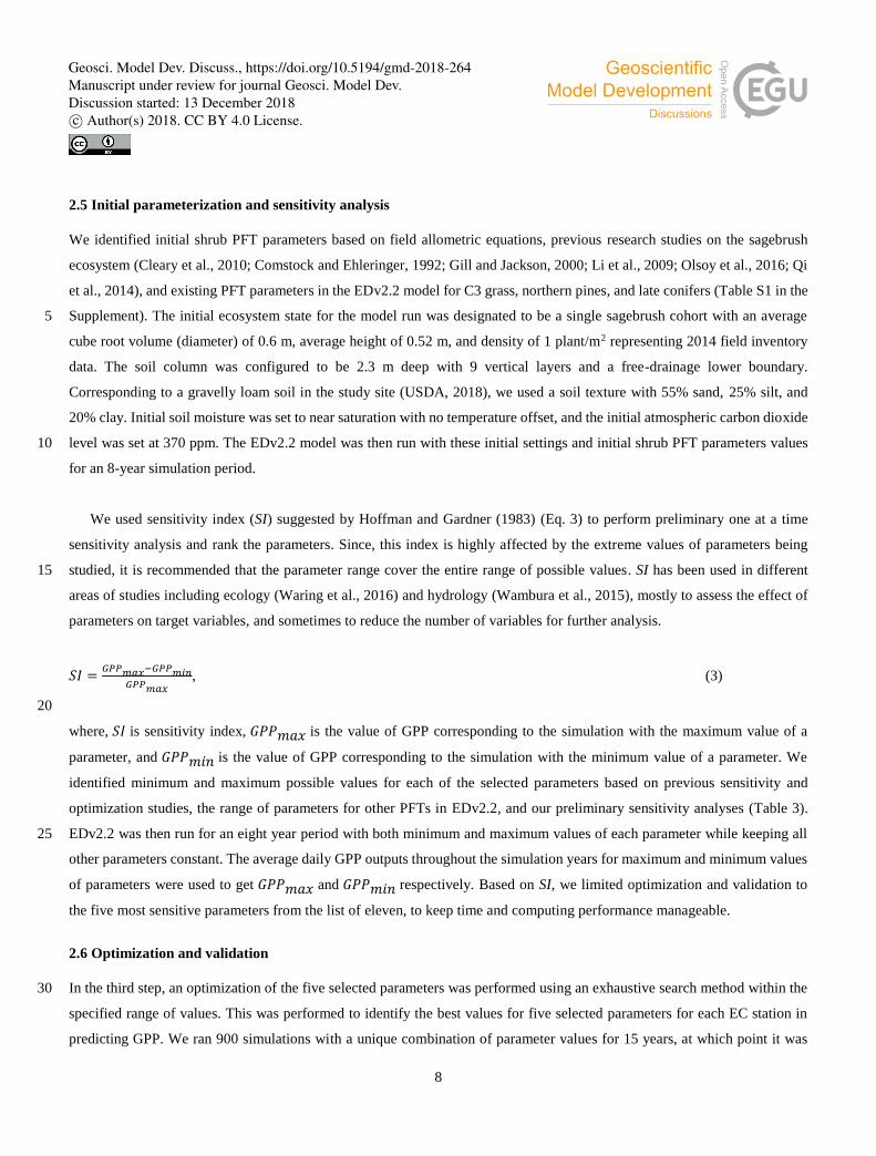
3.1 Initial parameterization and sensitivity analysis 20

For the model run based on the initial values of parameters (Table S1 of Supplement), the 8-year simulations produced an

annual cycle in GPP that decreases in amplitude during the initial 1-3 years, and remains at a level of approximately 0.07

KgC/m2/yr in the remaining years (Fig. 2a). Observed GPP in 2016 were 0.51 KgC/m2/yr and 0.38 KgC/m2/yr for the LS and

WBS sites, respectively. This result was significantly lower than the observed GPP from either of the EC sites, and thus

warranted changes in initial values for one or more parameters. 25

Based on the SI ranking, 𝑉𝑚0, 𝑆𝐿𝐴, stomatal slope, fine root turnover rate, and Q-ratio were identified as the top five

sensitive parameters compared to the other parameters explored (Fig. 2; Table 3). Related studies (Dietze et al., 2014; Medvigy

et al., 2009; Pereira et al., 2017; Zaehle et al., 2005) have also identified similar model parameters being important in estimating

GPP. In our study, higher parameter values of SLA, 𝑉𝑚0, and stomatal slope, resulted in higher GPP estimates (Fig. 2b and d),

whereas for fine root turnover rate and Q-ratio, higher parameter values produced lower GPP (Fig. 2e and f). The impact of 30

shifts in SLA, 𝑉𝑚0, and stomatal slope values are observed from the very beginning of the simulations, while changes in fine


10

root turnover rate and Q-ratio parameters start to show differences from roughly 3-4 years after the initial model run. Although

not ranked in the top five, leaf turnover rate, cuticular conductance, and growth respiration factor also had considerable

influences over GPP (Table 3).

Figure 2. Simulated daily GPP outputs from 1-8 years for the study location with (a) initial values of all five parameters, and 5

(b-f) maximum (green), minimum (blue), and initial (red) parameter values for SLA, 𝑉𝑚0, stomatal slope, Q-ratio, and fine

root turnover rate.

Table 3. PFT parameters in EDv2.2 used for the sensitivity analysis ranked according to Sensitivity Index (SI). Top five

parameters denoted by * were selected for optimization. 10

Parameters Initial Min Max SI Reference

SLA (m2kg-1) 4.5 2 15 0.973* Barbec (2014);

Wright et al., (2004)

𝑉𝑚0 (µmolm-2s-1) 16.5 4 30 0.962* Comstock & Ehlenger (1992);

Oleson et al., (2013)

Stomatal Slope 7 2 15 0.951* Dietze et al., (2014)

Ratio of fine roots to leaves/ Q-ratio 3.2 0.4 12 0.801* Dietze et al., (2014)

Fineroot Turnover rate (a-1) 0.33 0.1 2 0.787* Gill and Jackson, (2000)

Leaf Turnover rate (a-1) 1 0.1 2 0.728 *


11

Growth respiration factor 0.33 0.11 0.66 0.718 Wang et al., (2013)

Cuticular conductance (µmolm-2s-1) 103 102 107 0.501 Barnard and Bauerle (2013):

Duursma et al., (2018)

Water Conductance (ms-1kgCroot-1) 1.9 × 10-5 1.9 × 10-6 1.9 × 10-4 0.227 *

Storage turnover 0.624 0.33 0.95 0.004 *

Leaf width (m) 0.05 0.01 0.10 0.002 *

* Information about the range comes from range of values for other PFTs in EDv2.2, and our preliminary sensitivity analysis

3.2 Optimization and validation

For our exhaustive search of parameter values, we limited search domains for parameters based on previous studies and the

result of our sensitivity analysis. SLA search limits were largely based on Olsoy et al. (2016), who suggested a range of 3 to 6

m2/Kg for sagebrush SLA, but who also hinted at variation due to regional and seasonal variation. Similarly, limits for 5

𝑉𝑚0 were extended slightly beyond Comstock and Ehleringer’s (1992) recommendations for Great Basin shrubs, and the upper

limit for stomatal slope was extended slightly beyond that used by Oleson et al. (2013) for a shrub PFT in the Community

Land Model (CLMv4.5). We set search domains for Q-ratio based on a leaf and root biomass study of sagebrush by Cleary et

al. (2010), and fine root turnover ratio was based on results from a study on Artemisia ordosica in a semi-arid region of China

(Li et al, 2009). Interval distances (or ‘steps’) were calculated to equally space out the range between the maximum and 10

minimum of each parameter for a given number of intervals (Table 4). Parameters identified as exerting more control on GPP

prediction were assigned higher number of steps, resulting in the following: five steps of SLA and 𝑉𝑚0, four steps for stomatal

slope, and three steps for Q-ratio and fine root turnover rate. Among 900 simulations for unique parameter value combinations,

180 cases which did not provide model optimization results because of numerical instabilities (with GPP approaching zero),

were excluded from subsequent analysis. 15

Table 4. Minimum value, maximum value, interval size, and number of steps for each parameter used in optimization.

Parameter Min Max Interval Number of steps

SLA (m2kg-1) 3.00 9.00 1.50 5

𝑉𝑚0 (µmolm-2s-1) 11.50 21.50 2.50 5

Stomatal slope 7.00 10.00 1.00 4

Fine root turnover (a-1) 0.11 0.33 0.11 3

Q-ratio 0.40 3.20 1.40 3

We selected ten simulations with the best NSE scores for both LS and WBS sites (Table S2 and Fig. S1 in the Supplement)

and determined ensemble means of parameter values for these sites (Table 5). We then ran EDv2.2 to predict GPP using 20

ensemble mean parameter values for each of the EC stations (hereafter, the ‘ensemble case’). Among the ten best simulations


12

selected for each EC sites, two of them were commonly selected in both sites. One of them was ranked top with highest NSE

score (hereafter, the ‘best case’) and the other one was ranked as top fifth for LS and top second for WBS site. Both of these

common simulations, showed gradual growth of C3 grass through the simulation years even though we initialized model with

only shrub PFT. In the final year of simulation, the ‘best case’ had about 51% of total GPP coming from C3 grass and the other

one had about 43% from it (Table S2 and Fig. S2 in the Supplement). Optimized parameter values were considerably different 5

between the best case and ensemble cases for both stations, possibly suggesting interaction effects among the parameters

(Table 5). When parameters from ensemble means between two stations were compared, mean 𝑉𝑚0 for LS was higher by 3

µmolm-2s-1 than that for WBS. Mean parameter for stomatal slope was lower by 1 for LS than for WBS site. Another clear

difference was with ensemble mean for Q-ratio which was higher by 0.70 for LS than for WBS. But, we did not find such

differences for SLA and fine root turnover rate. 10

Figure 3. Optimization of daily GPP (KgC/m2/yr) for water year 2016 based on EC station observation data from a) LS and

b) WBS EC towers. Spring is shown as roughly 170-255 DOY.

15

Figure 3 compares simulated GPP from the final modeled year (from the ten best simulations and the ensemble case) with

the observed GPP in 2016 from each EC station. Optimization results for the LS site in Fig. 3a show that simulated GPP

matches well with observed data for most days, except during the spring, during which a clear peak in observed GPP was not

captured by the simulation results. A lower spring peak in GPP was observed at the WBS site (Fig. 3b) and was far more

comparable to simulation results. The impact of the spring mismatch in the LS site was such that, despite some over-prediction 20

during the fall season for WBS simulations, Bias and NSE were better for WBS than for LS data (Table 5). However, for both

EC site comparisons, most simulations resulted in a negative bias, and optimization NSEs for the ensemble cases were not as

good as for the best cases.


13

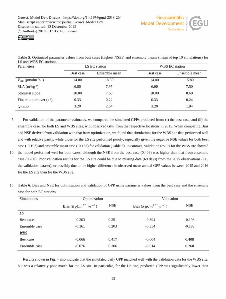
Table 5. Optimized parameter values from best cases (highest NSEs) and ensemble means (mean of top 10 simulations) for

LS and WBS EC stations.

Parameters LS EC station WBS EC station

Best case Ensemble mean Best case Ensemble mean

𝑉𝑚0 (µmolm-2s-1) 14.00 18.50 14.00 15.80

SLA (m2kg-1) 6.00 7.95 6.00 7.50

Stomatal slope 10.00 7.60 10.00 8.60

Fine root turnover (a-1) 0.33 0.22 0.33 0.24

Q-ratio 3.20 2.64 3.20 1.94

For validation of the parameter estimates, we compared the simulated GPPs produced from; (i) the best case, and (ii) the 5

ensemble case, for both LS and WBS sites, with observed GPP from the respective locations in 2015. When comparing Bias

and NSE derived from validation with that from optimization, we found that simulations for the WBS site data performed well

and with relative parity, while those for the LS site performed poorly, especially given the negative NSE values for both best

case (-0.193) and ensemble mean case (-0.183) for validation (Table 6). In contrast, validation results for the WBS site showed

the model performed well for both cases, although the NSE from the best case (0.408) was higher than that from ensemble 10

case (0.260). Poor validation results for the LS site could be due to missing data (69 days) from the 2015 observations (i.e.,

the validation dataset), or possibly due to the higher difference in observed mean annual GPP values between 2015 and 2016

for the LS site than for the WBS site.

Table 6. Bias and NSE for optimization and validation of GPP using parameter values from the best case and the ensemble 15

case for both EC stations.

Simulations Optimization

Validation

Bias (𝐾𝑔𝐶𝑚2−1𝑦𝑟−1) NSE

Bias (𝐾𝑔𝐶𝑚2−1𝑦𝑟−1) NSE

LS

Best case -0.203 0.251

-0.394 -0.193

Ensemble case -0.161 0.203

-0.354 -0.183

WBS

Best case -0.066 0.417

-0.004 0.408

Ensemble case -0.076 0.306

-0.014 0.260

Results shown in Fig. 4 also indicate that the simulated daily GPP matched well with the validation data for the WBS site,

but was a relatively poor match for the LS site. In particular, for the LS site, predicted GPP was significantly lower than


14

observed for most of the spring and summer months (Fig. 4c). The validation data (from 2015) for the LS site had clearly

higher GPP values for late summer days (Fig. 4a and c), thus resulting in higher negative Bias and negative NSE compared to

the optimization results. Predicted daily GPP for this site during the remaining months, however, is comparable with observed

values. In contrast, predicted daily GPP for the WBS site matched well with the validation GPP data through most of the year

(Fig. 4b and d), with slight inconsistencies during September (under estimation) and October (over estimation). Compared to 5

the best case, the ensemble case simulation for the LS site performed slightly better for most months, much better for July and

August, but worse for October and November (Fig. 4c). For the WBC site (Fig. 4d), the clearest differences between the two

cases were for April, May, July, and August, during which the best case simulation strongly outperformed the ensemble case.

Figure 4. Validation of GPP (KgC/m2/yr) using best case and ensemble case against respective EC station observation data 10

from water year 2015. a) daily GPP for LS, b) daily GPP for WBS, c) monthly GPP for LS, and d) monthly GPP for WBS.


15

4 Discussion

Our sensitivity analysis results were similar to previous studies (Dietze et al., 2014; LeBauer et al., 2013; Medvigy et al.,

2009), wherein parameters 𝑉𝑚0, SLA, fine root turnover rate, and stomatal slope were found to be the most influential in

determining carbon flux or primary productivity. A high variation in parameter values was observed among the simulations

that resulted in the best NSE values (Table S2 in the Supplement). The effects of some parameters on GPP prediction were not 5

the same when altered individually or simultaneously with other parameters. For instance, the sensitivity analysis showed an

increase in GPP with an increase in 𝑉𝑚0 (Fig. 2) and, since our initial GPP prediction was very low, we would expect higher

𝑉𝑚0 for better prediction. However, when all five parameters were optimized simultaneously, a generally lower value of

𝑉𝑚0 produced the best NSE (Table 5). Likewise, despite the sensitivity analysis suggesting higher GPP with lower fine root

turnover ratio and Q-ratio, the best results were obtained with the same initial values (maximum values in the search domain) 10

for these parameters, Nonetheless, top ten best parameter combinations exhibited greater variation of these parameters for

either EC site, and resulted in slightly lower mean values than the initial ones. This suggests interaction effects are dominant

over first order effects of the studied parameters, and there is likely nonlinear dependence among them.

GPP simulations from this study demonstrated a closer similarity with observations from the WBS site compared to the LS

site, even though the WBS EC station is outside of the WRF pixel used in this analysis. This could be due to slight differences 15

in soils and hydraulic conditions in the field compared to those conditions used for initialization. Moreover, variation between

morphological characteristics of the vegetation at the LS and WBS EC towers (characterized by low sagebrush and Wyoming

big sagebrush, respectively), such as differences in common plant heights and flowering seasons, may have resulted in the

observed differences in GPP (Howard, 1999; USDA, 2018). Since Wyoming big sagebrush is the dominant species in the

Reynold Creek Watershed area (Seyfried et al., 2000), meteorological forcing data used in this simulation, as well as the 20

allometric equations fitted for sagebrush (representing most areas of RCEW), could be favoring the more realistic growth

pattern of this species in the model (e.g., Fig. 3 and 4).

Additionally, differences in the phenology of the associated grass species between the two sites could result in differences

in seasonal and annual productivity (Cleary et al., 2015). For instance, the perennial grass at the LS site is Sandberg bluegrass,

which is photosynthetically active in early spring and senesces by early summer (USDA, 2016), and thus may have contributed 25

to observed spring GPP peak at the LS site. In contrast, the associated grass at the WBS site, bluebunch wheatgrass, does not

typically senesce by early summer. Indeed, the best optimization result from this study showed a gradual increase in C3 grass

through the years along with the shrubs, with about 51% of GPP coming from the former by the final year. We could not

validate how close this result was in terms of the actual species composition and ecosystem dynamics of the EC sites, as we

did not have GPP observations for unique PFTs. However, the emphasis of this study was to optimize shrub PFT parameters, 30

rather than C3 grass PFT parameters for the study area. Although we would expect that simultaneous optimization of both

grass and shrub PFTs would result in improved representation of the vegetation composition in the study area, it would also

increases the number of parameters required, potentially complicating the process of optimization and validation unique to


16

each PFT. Moreover, several studies suggest that the parameters 𝑉𝑚0 and SLA vary considerably across seasons (Groenendijk

et al., 2011; Kwon et al., 2016; Olsoy et al., 2016; Zhang et al., 2014). The mismatch in daily GPP pattern between simulated

and flux tower data for specific seasons could be partly attributed to the lack of the model’s ability to address these seasonal

deviations correctly. Like most other terrestrial biosphere models, EDv2.2 does not incorporate seasonal variation in 𝑉𝑚0,

SLA, or other model parameters (Medvigy et al., 2009). Finally, we can achieve better results in parameter optimization and 5

GPP prediction of sagebrush ecosystem, by making some advances in our methods. We can adopt some robust sensitivity

(including variance decomposition, first order and second order analysis) (Zhang et al., 2017) and optimization (including cost

function, gradient descent, and uncertainty analysis) (Richardson et al., 2010) methods to fine tune the sagebrush PFT

parameters. Similarly, instead of relying on a single year of observation data for optimization and/or validation, we can use

multiple years of data that would take into account the inter annual variability normally observed in ecosystem fluxes. 10

5 Conclusions

In this study, the Ecosystem Demography (EDv2.2) model was used to parameterize shrub PFT parameters and predict GPP

for a sagebrush ecosystem in the Great Basin. Initial shrub PFT parameters were identified based on allometric equations fitted

with field data, previous studies on sagebrush and shrubs in the sagebrush-steppe, and other PFTs (C3 grass, northern pines,

and late conifers) in EDv2.2. The WRF model was used to acquire and force simulation with meteorological inputs to predict 15

GPP. The simulation with initial shrub PFT parameters showed annual decline in GPP for 1-3 years and remained at a low

level (compared to observed GPP data) for the remaining simulation period. Sensitivity analysis suggested Vm0, SLA, stomatal

slope, fine root turnover rate, and Q-ratio ranked top five in influencing GPP prediction, which agrees with previous studies.

An exhaustive search was performed over constrained domains to explore the optimum combination of parameters to predict

GPP. This led to identification of parameter values for best case and ensemble mean (of the ten best cases) cases optimized for 20

the LS and WBS EC sites, using the NSE. Even though the model predicted daily GPP quite well, mostly negative bias was

observed in predictions, and there was mismatch during the spring months. Validation results showed better performance by

parameters optimized for WBS site than those done for LS site in GPP prediction. The difference in the local site vegetation

community and the overall dominance of Wyoming big sagebrush in the study area and in the Great Basin may explain why

the GPP predictions were closest to the WBS site. Similarly, the limitation of EDv2.2 in incorporating seasonal variation of 25

parameters like Vm0 and SLA, could also be attributed to its poor predictions for spring seasons.

Our identification of coefficients for allometric equations coupled with the other parametrization of a semiarid shrub PFT

for EDv2.2 will permit exploration of additional research questions. For instance, we can run EDv2.2 at regional scales with

optimized parameters to model the spatiotemporal dynamics of sagebrush community composition and ecosystem flux, under

different climate and ecological restoration scenarios. Another direction is to optimize C3 grass PFT parameters in EDv2.2, 30

simultaneously with shrub PFT parameters, by using multiple years of observation data to characterize inter annual variation.


17

Code & data availability. Original EDv2.2 is available at Github (https://github.com/EDmodel/ED22), which is maintained

and continuously updated by the owners of the repository. Modified source codes for EDv2.2 with shrub PFT parameters used

in this paper and input data are available at https://doi.org/10.5281/zenodo.2144044 (Last access: 12 December, 2018).

Author contribution. KP led the model simulation and manuscript preparation with significant contributions from all co-5

authors. KP, HD, NFG, ANF, KCM, and DJS conceived the idea and contributed in research design. KP, KCM, and HD led

work on fitting shrub allometric equations and sagebrush parameters, with feedback from all other authors. GNF and AWF

processed EC tower data to use in the analysis.

Competing interests. The authors declare that they have no conflict of interest. 10

Acknowledgements. This work was supported by the Joint Fire Science Program grant (Project ID: 15-1-03-23), NASA

Terrestrial Ecology (NNX14AD81G), and NSF Reynolds Creek CZO project (58-5832-4-004). We thank Nayani T.

Ilangakoon and Lucas P. Spaete from Boise Center Aerospace Laboratory (BCAL), Boise State University; Dr. Matt Masarik

from Lab for Ecohydrology and Alternative Futuring (LEAF), Boise State University; and the staff at Research Computing, 15

Boise State University. Part of this work was performed at R2 computer cluster, Boise State University. Authors are thankful

to Dr. Paul R. Moorcroft, Center for the Environment, Harvard University; Dr. David Medvigy, Department of Biological

Sciences, University of Notre Dame; Dr. Ryan G. Knox, Earth Science Division, Lawrence Berkley National Laboratory; and

Dr. Michael Dietze, Earth and Environment Department, Boston University for valuable inputs in exploring shrub PFT

parameters. We also thank Dr. Matthew Germino and Dr. David Barnard for expert review of the input parameters and review 20

of the manuscript, respectively. Any use of trade, product, or firm names is for descriptive purposes only and does not imply

endorsement by the U.S. Government.

References

AmeriFlux: http://ameriflux.lbl.gov, last access: 7 May 2018.

Antonarakis, A. S., Munger, J. W., and Moorcroft, P. R.: Imaging spectroscopy- and lidar-derived estimates of canopy 25

composition and structure to improve predictions of forest carbon fluxes and ecosystem dynamics, Geophys. Res. Lett., 41,

2535–2542, doi:10.1002/2013GL058373, 2014.

Barnard, D. M., and Bauerle, W. L.: The implications of minimum stomatal conductance on modeling water flux in forest

canopies, Journal of Geophysical Research: Biogeosciences, 118, 1322-1333, doi:10.1002/jgrg.20112, 2013.

Bond-Lamberty, B., Fish, J., Holm, J. A., Bailey, V. and Gough, C. M.: Moderate forest disturbance as a stringent test for gap 30

and big-leaf models. Biogeosciences Discuss, 11, 11217-11248, 2014.


18

Botkin, D. B., Janak, J.F., Wallis, J. R.: Rationale, Limitations, and Assumptions of a Northeastern Forest Growth Simulator.

IBM Journal of Research and Development, 16(2), 101-116, 1972.

Brabec, M. M.: Big Sagebrush (Artemisia tridentata) in a shifting climate context: assessment of seedling responses to climate,

Master’s Thesis. Boise State University, United States, 116pp., 2014.

Bradley, B. A.: Assessing ecosystem threats from global and regional change: hierarchical modeling of risk to sagebrush 5

ecosystems from climate change, land use and invasive species in Nevada, USA. Ecography, 33, 198-208, 2014.

Braswell, B. H., Sacks, W. J., Linder, E., and Schimel, D. S.: Estimating diurnal to annual ecosystem parameters by synthesis

of a carbon flux model with eddy covariance net ecosystem exchange observations. Global Change Biology, 11, 335–355,

doi:10.1111/j.1365-2486.2005.00897.x, 2005.

Chambers, J. C., Miller, R. F., Board, D. I., Pyke, D. A., Roundy, B. A., Grace, J. B., Schupp, E. W., and Taush, R. J. 10

Resilience and Resistance of Sagebrush Ecosystems: Implications for State and Transition Models and Management

Treatments. Range Ecol Manage 67: 440-454, 10.2111/REM-D-13-00074.1, 2010.

Chen, J. M., Mo, G., Pisek, J., Liu, J., Deng, F., Ishizawa, M., and Chan, D.: Effects of foliage clumping on the estimation of

global terrestrial gross primary productivity, Global Biogeochem. Cycles, 26, GB1019, doi:10.1029/2010GB003996, 2012.

Cleary, M. B., Pendall, E., and Ewers, B. E.: Aboveground and belowground carbon pools after fire in mountain big sagebrush 15

steppe, Rangel Ecol. Manag., 63, 187–96, doi.org/10.2111/REM-D-09-00117.1, 2010.

Cleary, M. B., Naithani, K. J., Ewers, B.E., and Pendall, E.: Upscaling CO2 fluxes using leaf, soil and chamber measurements

across successional growth stages in a sagebrush steppe ecosystem, J. Arid Environ., 121, 43–51, 2015.

Comstock, J.P. and Ehleringer, J.R.: Plant adaptation in the Great Basin and Colorado Plateau, Great Basin Naturalist, 52, 195-

215, 1992. 20

Connelly, J. W., Knick, S. T., Schroeder, M. A., and Stiver, S. J.: Conservation Assessment of Greater Sage-grouse and

Sagebrush Habitats. Western Association of Fish and Wildlife Agencies, Unpublished Report, Cheyenne, Wyoming, 2004.

Davidson, E., Lefebvre, P. A., Brando, P. M., Ray, D. M., Trumbore, S. E.,Solorzano, L. A., Ferreira, J. N., Bustamante, M.

M. da C., and Nepstad, D. C.: Carbon inputs and water uptake in deep soils of an eastern Amazon forest, Forest Science,

57, 51–58, doi.org/10.1093/forestscience/57.1.51, 2011. 25

Dietze, M. C., Serbin, S. P., Davidson, C., Desai, A. R., Fend, X., Kelly, R., Kooper, R, LeBauer, D., Mantooth, J., McHenry,

K., and Wang, D.: A quantitative assessment of a terrestrial biospheremodel’s data needs across North American biomes,

J. Geophys. Res.Biogeosci., 119, 286 –300, doi:10.1002/2013JG002392, 2014.

Dong, J., Li, L., Shi, H., Chen, X., Luo, G., and Yu, Q.: Robustness and Uncertainties of the “Temperature and Greenness”

Model for Estimating Terrestrial Gross Primary Production, Scientific Reports, 7, 44046, 2017. 30

Duursma, R. A., Blackman, C. J., Lopez, R., Martin-StPaul, N. K., Cochard, H., Medlyn, B. E.: On the minimum leaf

conductance: its role in models of plant water use, and ecological and environmental controls, New Phytologist, online

version, doi : 10.1111/nph.15395, 2018.

Farquhar, G. D. and Sharkey T. D.: Stomatal conductance and photosynthesis, Ann. Rev. Plant Physiol., 33, 317– 345, 1982.


19

Fellows, A. W., Flerchinger, G. N., Seyfried, M. S., and Lohse, K.: Data for Partitioned Carbon and Energy Fluxes Within the

Reynolds Creek Critical Zone Observatory [Data set]. Retrieved from https://doi.org/10.18122/B2TD7V, 2017.

Fellows, A. W., Flerchinger, G. N., Lohse, K. A., and Seyfried, M. S.: Rapid Recovery of Gross Production and Respiration

in a Mesic Mountain Big Sagebrush Ecosystem Following Prescribed Fire, Ecosystems, 1-12, doi.org/10.1007/s10021-

017-0218-9, 2018. 5

Fisher, R., McDowell, N., Purves, D., Moorcroft, P., Sitch, S., Cox, P., Huntingford, C., Meir, P., and Woodward, F. I.:

Assessing uncertainties in a second-generation dynamic vegetation model caused by ecological scale limitations, New

Phytologist, 187, 666-681, doi: 10.1111/j.1469-8137.2010.03340.x, 2010.

Fisher, R. A., Koven, C. D., Anderegg, W. R. L, Christoffersen, B. O., Dietze, M. C., Farrior, C. E. Holm, J. A., Hurtt, G. C.,

Knox, R. G., Lawrence, P. J., Lichstein, J. W., Longo, M., Matheny, A. M., Medvigy, D., Muller-Landau, H. C., Powell, 10

T. L., Serbin, S. P., Sato, H., Shuman, J. K., Smith, B., Trugman, A. T., Viskari, T., Verbeeck, H., Weng, E., Xu, C., Xu,

X., Zhang, T., and Moorcroft, P. R.: Vegetation demographics in Earth System Models: A review of progress and priorities,

Glob. Change Biol., 24, 35-24, DOI: 10.1111/gcb.13910, 2017.

Flores, A., Masarik, M., and Watson, K.: A 30-Year, Multi-Domain High-Resolution Climate Simulation Dataset for the

Interior Pacific Northwest and Southern Idaho [Data set]. Retrieved from http://dx.doi.org/10.18122/B2LEAFD001, 2016. 15

Gill, R.A. and Jackson, R. B.: Global patterns of root turnover for terrestrial ecosystems, New Phytol., 147, 13-31,

doi.org/10.1046/j.1469-8137.2000.00681.x, 2000.

Glenn, N.F., Spaete, L. P., Shrestha, R., Li, A., Ilangakoon, N., Mitchell, J., Ustin, S. L., Qi, Y., Dashti, H., and Finan, K.:

Shrubland Species Cover, Biometric, Carbon and Nitrogen Data, Southern Idaho, 2014. ORNL DAAC, Oak Ridge,

Tennessee, USA. [Data set] retrieved from https://doi.org/10.3334/ORNLDAAC/1503, 2017. 20

Groenendijk, M., Dolman, A. J., Ammann, C., Arneth, A., Cescatti, A., Dragoni, D., Gash, J. H. C., Gianelle, D., Gioli, B.,

Kiely, G., Knohl, A., Law, B. E., Lund, M., Marcolla, B., Van Der Molen, M. K., Montagnani, L., Moors, E., Richardson,

A. D., Roupsard, O., Verbeeck, H., and Wohlfahrt, G. Seasonal variation of photosynthetic model parameters and leaf area

index from global Fluxnet eddy covariance data, J. Geophys. Res., 116, G04027, doi:10.1029/2011JG001742, 2011.

Gupta, H. V., Kling, H., Yilmaz, K. K., and Martinez, G. F.: Decomposition of the mean squared error and NSE performance 25

criteria: Implications for improving hydrological modelling, Journal of Hydrology, 377, 80-91,

doi:10.1016/j.jhydrol.2009.08.003, 2009.

Hoffman, E. O. and Gardner, R. H.: Evaluation of Uncertainties in Environmental Radiological Assessment Models, in: Till,

J. E. and Meyer, H. R. (Eds.): Radiological Assessments: a Textbook on Environmental Dose Analysis. Washington, DC:

U.S. Nuclear Regulatory Commission; Report No. NUREG/CR-3332, 1983. 30

Homer, C.G., Dewitz, J.A., Yang, L., Jin, S., Danielson, P., Xian, G., Coulston, J., Herold, N.D., Wickham, J.D., and Megown,

K. : Completion of the 2011 National Land Cover Database for the conterminous United States-Representing a decade of

land cover change information. Photogrammetric Engineering and Remote Sensing, v. 81, no. 5, p. 345-354, 2015


20

Howard, J. L. 1999. Artemisia tridentata subsp. Wyomingensis, in: Fire Effects Information System, [Online]. U.S. Department

of Agriculture, Forest Service, Rocky Mountain Research Station, Fire Sciences Laboratory (Producer). Retrieved from

https://www.fs.fed.us/database/feis/plants/shrub/arttriw/all.html, last access: 20 August 2018.

Huntzinger, D. N., Post, W. M., Wei, Y, Michalak, A. M., West, T. O., Jacobson, A. R., Baker, I. T., Chen, J. M., Davis, K.

J., Hayes, D. J., Hoffman, F. M., Jain, A. K., Liu, S., McGuire, A. D., Neilson, R. P., Potter, C., Poulter, B., Price, D., 5

Raczka, B. M., Tian, H. Q., Thornton P., Tomelleri, E., Viovy, N., Xiao, J., Yuan, W., Zeng, N., Zhao, M., and Cook, R.:

North American Carbon Program (NACP) regional interim synthesis: Terrestrial biospheric model intercomparison, Ecol.

Modell., 232, 144–157, doi:10.1016/j.ecolmodel.2012.02.004, 2012.

Kim, Y., Knox, R. G., Longo, M., Medvigy, D., Hutyra, L. R., Pyle, E. H., Wofsy, S. C., Bras, R. L., and Moorcroft, P. R.:

Seasonal carbon dynamics and water fluxes in an Amazon rainforest. Global Change Biology, 18, 1322-1334, doi: 10

10.1111/j.1365-2486.2011.02629.x, 2012.

Knick, S. T. and Dobkin, D. S.: Teetering on the Edge or Too Late? Conservation and Research Issues for Avifauna of

Sagebrush Habitats, The Condor, 105, 611-634, https://doi.org/10.1650/7329, 2003.

Knox, R. G., Longo. M., Swann. A. L. S., Zhang, K., Levine, N. M., Moorcroft, P. R., and Bras, R. L.: Hydrometeorological

effects of historical land-conversion in an ecosystem-atmosphere model of Northern South America, Hydrol. Earth Syst. 15

Sci., 19, 241–273, doi:10.5194/hess-19-241-2015, 2015.

Krause, P., Boyle, D. P., and Baise, F.: Comparison of different efficiency criteria for hydrological model assessment.

Advances in Geosciences, 5, 89-97, https://doi.org/10.5194/adgeo-5-89-2005, 2005.

Kwon, B., Kim, H. S., Jeon, J., and Yi, M. J.: Effects of Temporal and Interspecific Variation of Specific Leaf Area on Leaf

Area Index Estimation of Temperate Broadleaved Forests in Korea. Forests, 7, 215, doi:10.3390/f7100215, 2016. 20

LCC: Landscape Conservation Cooperatives: 2015 LCC Network Areas OGC Webservices :

https://www.sciencebase.gov/catalog/item/55c52e08e4b033ef5212bd75, last access, 21 April, 2018

LeBauer, D. S., Wang, D., Richter, K. T., Davidson, C. C., and Dietze, M. C.: Facilitating feedbacks between field

measurements and ecosystem models. Ecological Monographs, 83, 133-154, https://doi.org/10.1890/12-0137.1, 2013.

Leuning, R.: A critical appraisal of a combined stomatal-photosynthesis model for C3 plants, Plant Cell Environ., 18, 339– 25

355, 1995.

Li, C., Sun, O. J., Xiao, C., and Han, X.: Differences in Net Primary Productivity Among Contrasting Habitats in Artemisia

ordosica Rangeland of Northern China. Rangeland Ecol Manage., 62, 345-350, https://doi.org/10.2111/07-084.1, 2009.

McArthur, E. D. and Plummer, A. P.: Biogeography and management of native western shrubs: a case study, Section

Tridentatae of Artemisia, Great Basin Naturalist Memoirs, 2 , 15, https://scholarsarchive.byu.edu/gbnm/vol2/iss1/15, 1978. 30

McIver, J. and Brunson, M.: Multidisciplinary, Multisite Evaluation of Alternative Sagebrush Steppe Restoration Treatments:

The SageSTEP Project, Range Ecol. Manage., 67, 435-439, https://doi.org/10.2111/REM-D-14-00085.1, 2014.

Medvigy, D. M.: The state of the regional carbon cycle: Results from a coupled constrained ecosystem-atmosphere model,

Ph.D. Thesis, Harvard Univ., Cambridge, Mass., 2006.


21

Medvigy, D., Wofsy, S. C., Munger, J. W., Hollinger, D. Y., and Moorcroft, P. R.: Mechanistic scaling of ecosystemfunction

and dynamics in space and time: Ecosystem Demography model version 2, J. Geophys. Res., 114, G01002,

doi:10.1029/2008JG000812, 2009.

Medvigy, D., Jeong, S. J., Clark, K. L., Skowronski, N. S., and Schäfer, K. V. R.: Effects of seasonal variatio n of

photosynthetic capacity onthe carbon fluxes of a temperate deciduous forest, Journal of Geo-physical Research: 5

Biogeosciences, 118, 1703– 1714, , doi:10.1002/2013JG002421, 2013.

Mo, X., Chen, J. M., Ju, W., and Black, T. A.: Optimization of ecosystem model parameters through assimilating eddy

covariance flux data with an ensemble Kalman filter, Ecological Modelling, 217, 157–173,

https://doi.org/10.1016/j.ecolmodel.2008.06.021, 2008.

Moorcroft, P. R.: Recent advances in ecosystem-atmosphere interactions: an ecological perspective, Proceedings of the Royal 10

Society B-Biological Sciences, 270, 1215–1227, DOI: 10.1098/rspb.2002.2251, 2003.

Moorcroft, P. R., Hurtt, G. C., Pacala, S. W.: A method for scaling vegetation dynamics: the Ecosystem Demography model

(ED), Ecol. Monogr., 71, 557–586, https://doi.org/10.1890/0012-9615(2001)071[0557:AMFSVD]2.0.CO;2, 2001.

Nash, J. E. and Sutcliffe, J. V. River flow forecasting through conceptual models, Part I - A discussion of principles, J. Hydrol.,

10, 282–290, 1970. 15

NPS, 2018. Great Basin: Trees and Shrubs. National Park Service: https://www.nps.gov/grba/learn/nature/treesandshrubs.htm,

last access: 26 July 2018.

Oleson, K., Lawrence, D. M., Bonan, G. B., Drewniak, B., Huang, M., Koven, C. D., Levis, S., Li, F., Riley, W. J., Subin, Z.

M., Swenson, S. C., Thornton, P. E., Bozbiyik, A., Fisher, R., Heald, C. L., Kluzek, E., Lamarque, J.-F., Lawrence, P. J.,

Leung, L. R., Lipscomb, W., Muszala, S., Ricciuto, D. M., Sacks, W., Sun, Y., Tang, J., and Yang, Z.-L.: Technical 20

Description of version 4.5 of the Community Land Model (CLM), NCAR Technical Note NCAR/TN-503+STR, Boulder,

Colorado, 420 pp., 2013.

Olsoy, P. J., Mitchell, J. J., Levia, D. F., Clark, P. E., Glenn, N. F.: Estimation of big sagebrush leaf area index with terrestrial

laser scanning, Ecological Indicators, 61, 815–821, https://doi.org/10.1016/j.ecolind.2015.10.034, 2016.

Pacala, S. W., Canham, C. D., Silander Jr, J. A.: Forest models defined by field measurements. I. The design of a northeastern 25

forest simulator, Can. J. For. Res., 23, 1980-1988, 1993.

Pereira, F. F, Farinosi, F., Arias, M. E., Lee, E., Briscoe, J., and Moorcroft, P.R.: Technical note: A hydrological routing

scheme for the Ecosystem Demography model (ED+R) tested in the Tapajós River basin in the Brazilian Amazon, Hydrol.

Earth Syst. Sci., 21, 4629–4648, https://doi.org/10.5194/hess-21-4629-2017, 2017.

Qi, Y., Dennison, P. E., Jolly, W. M, Kropp, R. C., and Brewer, S. C.: Spectroscopic analysis of seasonal changes in live fuel 30

moisture content and leaf dry mass, Remote Sensing of Environment, 150, 198-206,

https://doi.org/10.1016/j.rse.2014.05.004, 2014.

Reichstein, M., Falge, E., Baldocchi, D., Papale, D., Aubinet M., Berbigier P., Bernhofer, C., Buchmann, N., Gilmanov, T.,

Granier, A., Grünwald, T., Havránková, K., Ilvesniemi, H., Janous, D., Knohl, A., Laurila, T., Lohila, A., Loustau, D.,


22

Matteucci, G., Meyers, T., Miglietta, F., Ourcival, J. M., Pumpanen, J., Rambal, S., Rotenberg, E., Sanz, M., Tenhunen, J.,

Seufert, G., Vaccari, F., Vesala, T., Yakir, D., and Valentini, R.: On the separation of net ecosystem exchange into

assimilation and ecosystem respiration: review and improved algorithm, Glob. Change Biol., 11, 1424–39,

https://doi.org/10.1111/j.1365-2486.2005.001002.x, 2005.

Richardson, A. D., Williams, M., Hollinger, D. Y., Moore, D. J. P., Dail, D. B., Davidson, E. A., Scott, N. A., Evans, R. E., 5

Hughes, H., Lee, J. T., Rodrigues, C., Savage, K.: Estimating parameters of a forest ecosystem C model with measurements

of stocks and fluxes as joint constraints, Oecologia, 164, 25–40, doi:10.1007/s00442-010-1628-y, 2010.

Schlaepfer, D. R., Lauenrotha, W. K., and Bradford, J. B.: Modeling regeneration responses of big sagebrush (Artemisia

tridentata) to abiotic conditions, Ecological Modelling, 286, 66-77, https://doi.org/10.1016/j.ecolmodel.2014.04.021, 2014.

Schroeder, M. A., Aldridge, C. L., Apa, A. D., Bohne, J. R., Braun, C. E., Bunnell, S. D., Connelly, J. W., Deibert, P. A., 10

Gardner, S. C., Hilliard, M. A., Kobriger, G. D., McAdam, S. M., McCarthy, C. W., McCarthy, J. J., Mitchell, D. L.,

Rickerson, E. V., and Stiver, S. J.: Distribution of Sage-Grouse in North America, The Condor, 106, 363-376,

https://doi.org/10.1650/7425, 2004.

Sellers, P. J., Berry, J. A., Collatz, G. J., Field, C. B., and Hall, F.G.: Canopy reflectance, photosynthesis, and transpiration.

III. A reanalysis using improved leaf models and a new canopy integration scheme, Remote Sensing of Environment, 42, 15

187-216, doi.org/10.1016/0034-4257(92)90102-P, 1992.

Seyfried, M. S., Harris, R., Marks, D., and Jacob, B.: A geographic database for watershed research: Reynolds Creek

Experimental Watershed, Idaho, USA, Tech. Bull. NWRC 2000-3, 26 pp., Northwest Watershed Res. Cent., Agric. Res.

Serv., U.S. Dep. of Agric., Boise, Idaho, 2000

Sitch, S., Smith, B., Prentice, I. C., Arneth, A., Bondeau, A., Cramer, W., Kaplans, J. O., Levis, S., Lucht, W., Sykes, M. T., 20

Thonicke, K. and Venevsky, S.: Evaluation of ecosystem dynamics, plant geography and terrestrial carbon cycling in the

LPJ dynamic vegetation model, Global Change Biol., 9, 161 – 185, 2003.

Smith, B., Trentice, C.I., and Sykes, M. T.: Representation of vegetation dynamics in the modelling of terrestrial ecosystems:

comparing two contrasting approaches within European climate space. Global Ecology & Biogeography, 10, 621-637,

2001. 25

Stephenson GR (Ed.): CZO Dataset: Reynolds Creek - Geology, Soil Survey, Vegetation, GIS/Map Data (1960-1970),

Retrieved from http://criticalzone.org/reynolds/data/dataset/3722/, last access: 18 May 2018.

Trugman, A. T., Fenton, N. J., Bergeron, Y., Xu, X., Welp, L. R., and Medvigy, D.: Climate, soil organic layer, and nitrogen

jointlydrive forest development after fire in the North American boreal zone, Journal of Advances in Modeling the Earth

System, 8, 1180–1209, doi:10.1002/2015MS000576, 2016. 30

Turner, D. P., Ritts, W. D., Cohen, W. B., Gower, S. T., Running, S. W., Zhao, M., Costa, M. H., Kirschbaum, A. A., Ham, J.

M., Saleska, S. R., Ahl, D. E.: Evaluation of MODIS NPP and GPP products across multiple biomes, Remote Sens.

Environ., 102, 282–292, doi:http://dx.doi.org/10.1016/j.rse.2006.02.017, 2006.


23

USDA: Plant materials Technical Note No. MT-114. Natural Resources Conservation Service, United States Department of

Agriculture, August 2016, 2016.

USDA: Soil Survey Staff, Natural Resources Conservation Service, United States Department of Agriculture. Web Soil

Survey. Retrieved from https://websoilsurvey.sc.egov.usda.gov/, last access: 28 March 2018.

USDA: The PLANTS Database (http://plants.usda.gov, 20 August 2018). National Plant Data Team, Greensboro, NC 27401-5

4901 USA, 2018.

Wamburaa, F. J., Ndombab, P. M., Kongob, V., Tumboc, S. D.: Uncertainty of runoff projections under changing climate in

Wami River sub-basin, Journal of Hydrology: Regional Studies, 4, 333–348, 2015.

Wang, D., LeBauer, D., Dietze, M.: Predicting yields of short-rotation hybrid poplar (Populus spp.) for the United States

through model–data synthesis, Ecological Applications, 23(4), 944-958, 2013. 10

Waring, B. G., Averill, C., Hawkes, C. V.: Differences in fungal and bacterial physiology alter soil carbon and nitrogen cycling:

insights from meta-analysis and theoretical models, Ecology Letters, 16, 887-894, doi: 10.1111/ele.12125, 2016

Weiss, A. and Norman, J. M.: Partitioning solar radiation into direct and diffuse, visible and near-infrared components. Agric.

Forest Meteorol., 34, 205–213, 1985.

Zaehle, S., Sitch, S., Smith, B., and Hatterman, F.: Effects of parameter uncertainties on the modeling of terrestrialbiosphere 15

dynamics, Global biogeochemical cycles, 19, 3, DOI: 10.1029/2004GB002395, 2005.

Zhang, K., de Almeida Castanho, A. D., Galbraith, D. R., Moghim, S., Levine, N. M., Bras, R. L., Coe, M. T., Costa, M. H.,

Malhi, Y., Longo, M., Knox, R. G., McKnight, S., Wang, J.,and Moorcroft, P. R.: The fate of Amazonian ecosystems over

the coming century arising from changes in climate, atmospheric CO2, and land use, Glob. Change Biol., 21, 2569–2587,

https://doi.org/10.1111/gcb.12903, 2015. 20

Zhang, K., Ma. J., Zhu, G., Ma, T., Han, T., Feng, L. L.: Parameter sensitivity analysis and optimization for a satellite-based

evapotranspiration model across multiple sites using Moderate Resolution Imaging Spectroradiometer and flux data, J.

Geophys. Res. Atmos., 122, 230–245, doi:10.1002/2016JD025768, 2017

Zhang, Y, Guanter, L., Berry, J. A., Joiner, J., Tol, C. V. D., Huete, A., Gitelson, A., Voigt, M., and Kohler, P.: Estimation of

vegetation photosynthetic capacity from space-based measurements of chlorophyll fluorescence for terrestrial biosphere 25

models, Global Change Biology, 20, 3727–3742, doi: 10.1111/gcb.12664, 2014.

Zhao, M. and Running, S. W.: Drought-Induced Reduction in Global Terrestrial Net Primary Production from 2000 through

2009, Science, 329, 940-943, doi: 10.1126/science.1192666, 2010.

Zhao, M., Heinsch, F. A., Nemani, R. R., Running, S. W.: Improvements of the MODIS terrestrial gross and net primary

production global data set, Remote Sens. Environ., 95, 164–176, doi:http://dx.doi.org/10.1016/j.rse.2004.12.011, 2005. 30


Documents

Optimizing shrub parameters to estimate gross … based models like LPJ -DGVM (Lund -Potsman -Jena Dynamic Vegetation Model) (S itch et al., 2003) , and B IOME BGC (Running and Hunt,