Optimizing Space Utilization in Block Stacking Warehouses · PDF file2/9/2016 · stacking warehouse where the objectives are maximizing space utilization and minimizing trans-portation

February 9, 2016 International Journal of Production Research Manuscript

To appear in the International Journal of Production ResearchVol. 00, No. 00, 00 Month 20XX, 1–20

Optimizing Space Utilization in Block Stacking Warehouses

Shahab Derhamia∗ , Jeffrey S. Smitha and Kevin R. Gueb

aIndustrial & Systems Engineering, Auburn University, Auburn, AL 36849, USA; bIndustrial Engineering,

University of Louisville, Louisville, KY 40292, USA

(Received 00 Month 20XX; accepted 00 Month 20XX)

Block stacking storage is an inexpensive storage system widely used in manufacturing systems wherepallets of stock keeping units (SKUs) are stored in a warehouse at the finite production rates. However,determining the optimal lane depth that maximizes space utilization under a finite production rateconstraint has not been adequately addressed in the literature and is an open problem. In this research,we propose mathematical models to obtain the optimal lane depth for single and multiple SKUs wherethe pallet production rates are finite. A simulation model is used to evaluate performance of the proposedmodels under stochastic uncertainty in the major production parameters and the demand.

Keywords: block stacking; facility layout; warehouse design; space utilization

1. Introduction

Optimizing space utilization has been one of the main goals in designing and operating warehouses(Van den Berg 1999). The U.S. Roadmap for Material Handling and Logistics recognizes low ware-house utilization as one of the main factors that propels companies, associations and governmentsto employ collaborative warehouses more in the next decade. It also predicts that requests for highspeed delivery or same-day delivery forces companies to build their warehouses and distributioncenters near major metropolitan area where real estate is very expensive and therefore efficient useof space becomes more important (Gue et al. 2014).

Various approaches from the design to the operational phase of a warehouse have been developedto better utilize storage space. Block stacking is an inexpensive and conventional storage systemwhose performance depends on the efficient use of space. It is a unit load storage system in whichpallets of stock keeping units (SKUs) are stacked on top of one another in lanes on the warehousefloor. Pallets are stacked to the maximum stacking height which depends on the conditions andheights of the pallets, load weights, safety limits, clearance height of the warehouse, and so on.No racking or storage facility is required for this system and it can be employed in any warehousewith wide floor space. This makes it an inexpensive storage system to implement but challengingto manage in terms of space planning.

Two major operating policies that are widely used to manage storage spaces in this system arededicated and shared storage policies. In the dedicated policy, lanes are dedicated to SKUs andonly pallets of the assigned SKU are allowed to be stored in a lane. So, a lane may remain emptyuntil it is replenished with its assigned SKU. On the other hand, lanes are not dedicated to anySKUs in the shared storage policy and they are available to all SKUs once they become empty.This policy utilizes space more efficiently than the former one though the order picking process isgenerally less efficient since the SKUs storage locations change over time and SKUs are assigned

∗Corresponding author. Email: [email protected]


0

2

4

6

8

10

12

0 20 40 60 80 100 120 140 160 180

Figure 1. Waste of space in Example 1

to the lanes based on their availability rather than convenience of their locations. However, sharedstorage is widely used in warehouses that deal with numerous SKUs and limited storage space.

The shared policy is operated with allowing or not allowing blockage. When the variety of SKUsis large but their inventory is small, assigning a lane to a single SKU is not justifiable and thereforedifferent SKUs have to be stored in the same lane. In this case, blockage is inevitable and the goalis to arrange SKUs such that the relocation costs are minimized. An example of such a case is thestorage space allocation problem in a marine container terminal (Yang and Kim 2006; Peteringand Hussein 2013; Jang, Kim, and Kim 2013; Carlo, Vis, and Roodbergen 2014). On the otherhand, when the inventories of the SKUs are big enough to justify assigning a lane to a single SKU,no blockage policy is enforced. In this case to avoid blockage and relocation, a lane is dedicated toa SKU once it occupies the first position of the lane. This case mainly occurs in the warehouseslocated in manufacturing systems or the distribution centers where plenty of pallets of differentSKUs are block-stacked. However, this restriction wastes storage spaces in a lane when it is filledor depleted as there will be some unoccupied pallet positions in the lane that are just available tothe pallets of the assigned SKU. This effect is termed honeycombing and waste associated with itis incurred to the system until a lane becomes entirely occupied or empty (Hudock 1998).

In addition to honeycombing, aisles also contribute to the overall wasted space. Aisles are re-quired to have access to the lanes but their devoted spaces are not directly used for storage.Warehouse designers aim to minimize these two types of waste to enhance space utilization in thewarehouse. The following example shows how waste of storage space is calculated in a lane.

Example 1. Consider a batch of 10 pallets of a SKU is stored in a lane of two pallets deep.Pallets are produced at the rate of (1/5) pallets per hour, stacked up to two pallets high anddepleted at the rate of (1/18) pallets per hour. Assume that an aisle with width equivalent totwo pallets is required to access the lane. Figure 1 shows waste of storage space generated in theinventory cycle time of this SKU. At time zero, waste is zero because an empty lane is available toall SKUs. At time five, the first pallet is stored in the lane and makes the three unoccupied palletpositions in the lane unavailable to the other SKUs. This is the honeycombing waste. Moreover,four pallet positions are dedicated to the aisle to provide accessibility to the lane. So, seven palletpositions are wasted at this time. At times 10 and 15, the next two pallets are stored in the laneand the total number of wasted positions decreases to six and then five pallets, respectively. Thefirst depletion event occurs at time 18 and increases the number of wasted positions to six. Thisprocedure continues until all 10 pallets are produced, stored in the lane, and depleted. The areaunder the waste plot in Figure 1 is the pallets-time waste of storage space during the inventorycycle time, and dividing it by 175 hours gives the average waste of storage space in the inventorycycle time which is 7.48 pallets.

Storing a batch of pallets in deep lanes increases the honeycombing waste, but the space requiredfor aisles decreases while the reverse is true for the shallow lanes. Hence, a trade-off between the

2


9.87

7.48 7.46*

7.91

7

8

9

10

1 2 3 4

Figure 2. Optimal lane depth in Example 1

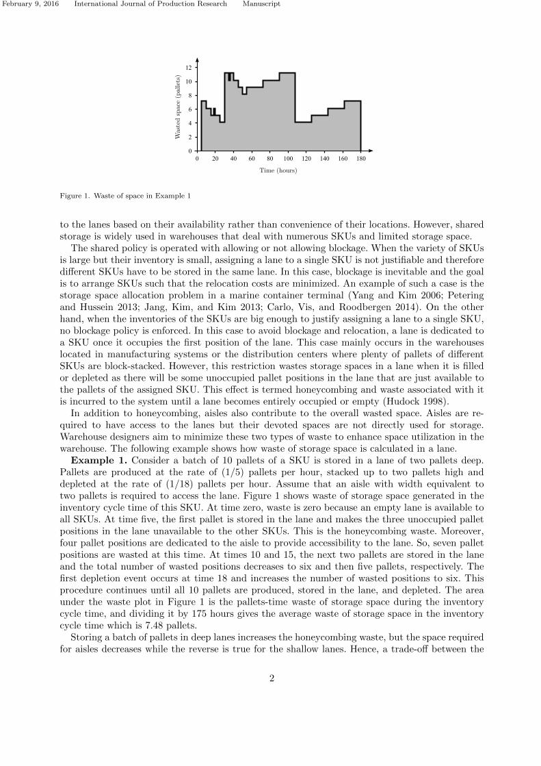
lane depth and width must be considered to optimize space utilization. This trade-off is shown inFigure 2 by comparing the average waste of storage space generated by storing the SKU describedin Example 1 in lanes with one to four pallets deep. In this case, the minimum waste achievedwhen the SKU is stored in the lanes with three pallets deep.

In this paper, we consider this trade-off from a mathematical point of view and develop models tocompute an optimal lane depth that minimizes waste of storage space in the warehouse. Our modelsare different from those existing in the literature in two major respects. First, the instantaneouspallet storage assumption, which was made in all previous research is relaxed and models arebuilt for finite production rates. Hence, they are more suitable for the warehouses located inmanufacturing systems where pallets are stored at finite production rates. Second, our proposedmodels aim to maximize utilization of the volume instead of the floor space. A review of the previousresearch on block stacking is provided in the next section.

2. Related research

Various studies have investigated designing the layout of a warehouse (Gu, Goetschalckx, andMcGinnis 2010). Most of them considered designing the layout with respect to the constructionand maintenance costs (Ashayeri, Gelders, and Wassenhove 1985; Rosenblatt, Roll, and Zyser1993; Pazour and Meller 2011), material handling costs in order picking process (Gue and Meller2009; Pohl, Meller, and Gue 2009; Omer Ozturkoglu, Gue, and Meller 2012, 2014; Ramtin andPazour 2014), products allocation (Heragu et al. 2005; Ramtin and Pazour 2015) and few of themconsidered objectives pertinent to the space utilization (Gue 2006). Extensive reviews on differentapproaches used to design different storage systems are found in Gu, Goetschalckx, and McGinnis(2010); Baker and Canessa (2009); Gu, Goetschalckx, and McGinnis (2007); Klose and Drexl (2005);Rouwenhorst et al. (2000). Studies that investigated space utilization in the block stacking storagesystems are reviewed in the following.

To the best of our knowledge, Kind (1975) was the first person who considered the trade-off between the lane depth and width in the block stacking storage and proposed a model toapproximately find the optimal lane depth that minimizes waste of storage space. He proposed thisapproximation for a single SKU whose batch of pallets are instantaneously stored in a warehouse.Marsh (1979) developed a simulation model to evaluate different storage and operating policies forblock-stacking. Later, Matson (1982) developed a more accurate version of Kind’s approximation(Kind 1975) for a single SKU and extended it to obtain the optimal common lane depth for multipleSKUs. Her models aim to maximize utilization of the floor space (area).

Goetschalckx and Ratliff (1991) showed that if a batch of pallets of a SKU is allowed to bestored in lanes with unlimited different depths, then the optimal lane depths follow a continuous

3


triangular pattern. They developed a continuous and discrete approximations to obtain the optimalmultiple lane depths considering limited and unlimited lane depths. They compared their proposedmodels with scenarios like equal lane depth models developed by Matson (1982) and two extremeheuristics in which a batch of pallets is stored in the lanes whose depths are equal to one or tothe batch size, respectively. They concluded space utilization is “relatively insensitive” to the lanedepth and all heuristic methods except the two extreme cases provide comparatively equivalentresults in terms of accuracy and computational complexity. However, their approaches, especiallythe one that assumes unlimited multiple lane depths, are not practical for multiple SKUs.

Larson, March, and Kusiak (1997) proposed a heuristic approach to design the layout of a blockstacking warehouse where the objectives are maximizing space utilization and minimizing trans-portation costs. Their class-based storage approach classifies SKUs based on the throughput to therequired storage space ratio, ranks classes based on their average ratios, and constructs and ded-icates the storage regions to the classes considering their ranks and required storage spaces. Thealgorithm considers honeycombing, fluctuations in the inventory level and the maximum stack-ing height to determine storage medium (i.e., racks or floor stacking) for a SKU, and assumesrandomized storage policy among the classes (storage zones).

Bartholdi (2014) developed Matson’s model to optimize volume utilization instead of the floorutilization. He suggested that maximizing the volume utilization is the better objective in thecurrent modern warehouse because volume within a warehouse is worth as much as floor space intoday’s modern warehouses.

All aforementioned studies assumed pallets of SKUs are instantaneously stored in a warehouse.In practice, this case occurs in a distribution center where trucks quickly unload pallets of SKUs,and hence it appears realistic to assume infinite arrival rate for incoming pallets. However, thisassumption cannot be justified in the warehouses located in manufacturing systems where palletsof SKUs are stored in the warehouse at finite production rates. In such a warehouse, waste ofstorage space is generated either when a lane is filled or depleted. However, the traditional modelsare not capable of taking the first part into account and therefore do not correctly compute theoptimal lane depth for such cases. We address this drawback in this paper by developing models todetermine the optimal lane depth for both single and multiple SKUs under the finite productionrate constraint.

3. Optimal lane depth

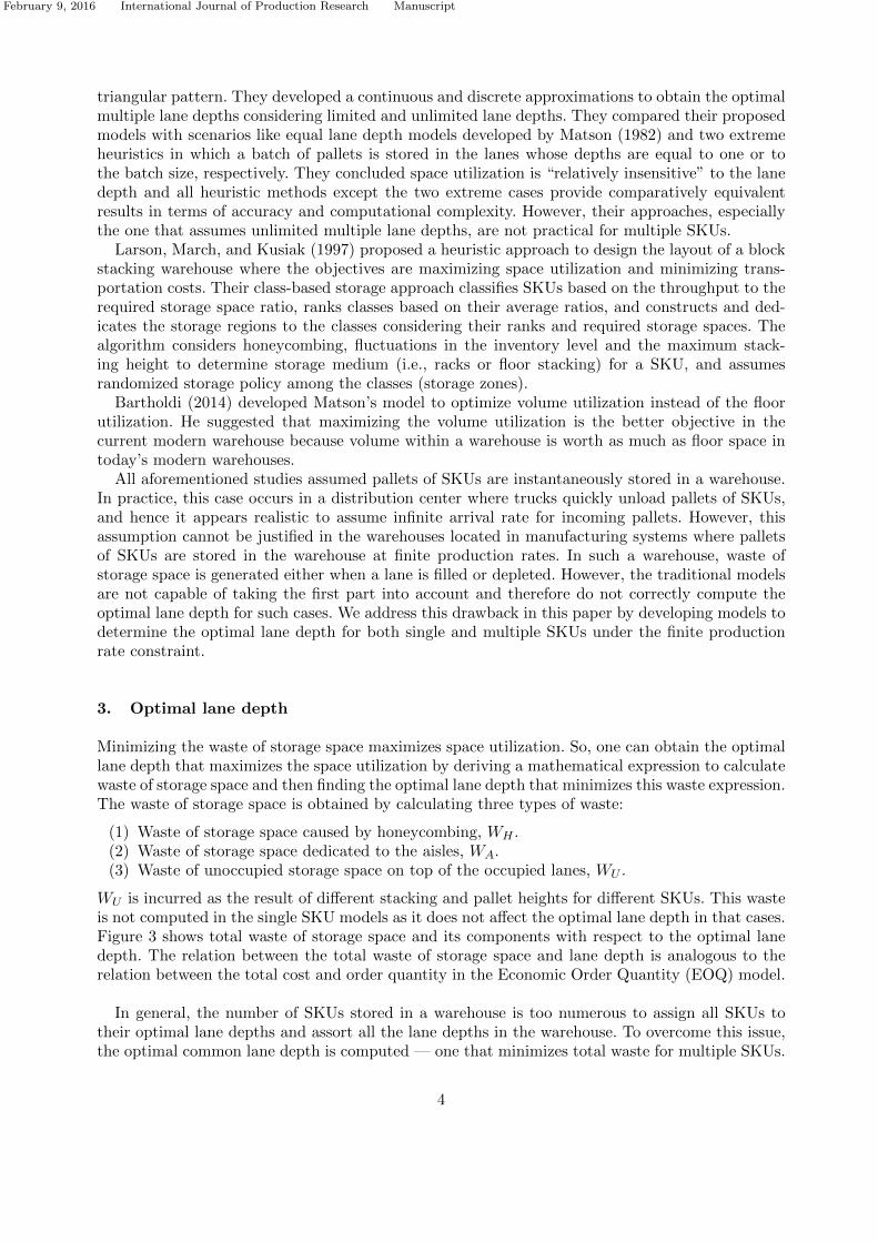
Minimizing the waste of storage space maximizes space utilization. So, one can obtain the optimallane depth that maximizes the space utilization by deriving a mathematical expression to calculatewaste of storage space and then finding the optimal lane depth that minimizes this waste expression.The waste of storage space is obtained by calculating three types of waste:

(1) Waste of storage space caused by honeycombing, WH .(2) Waste of storage space dedicated to the aisles, WA.(3) Waste of unoccupied storage space on top of the occupied lanes, WU .

WU is incurred as the result of different stacking and pallet heights for different SKUs. This wasteis not computed in the single SKU models as it does not affect the optimal lane depth in that cases.Figure 3 shows total waste of storage space and its components with respect to the optimal lanedepth. The relation between the total waste of storage space and lane depth is analogous to therelation between the total cost and order quantity in the Economic Order Quantity (EOQ) model.

In general, the number of SKUs stored in a warehouse is too numerous to assign all SKUs totheir optimal lane depths and assort all the lane depths in the warehouse. To overcome this issue,the optimal common lane depth is computed — one that minimizes total waste for multiple SKUs.

4


Figure 3. Total waste of storage space

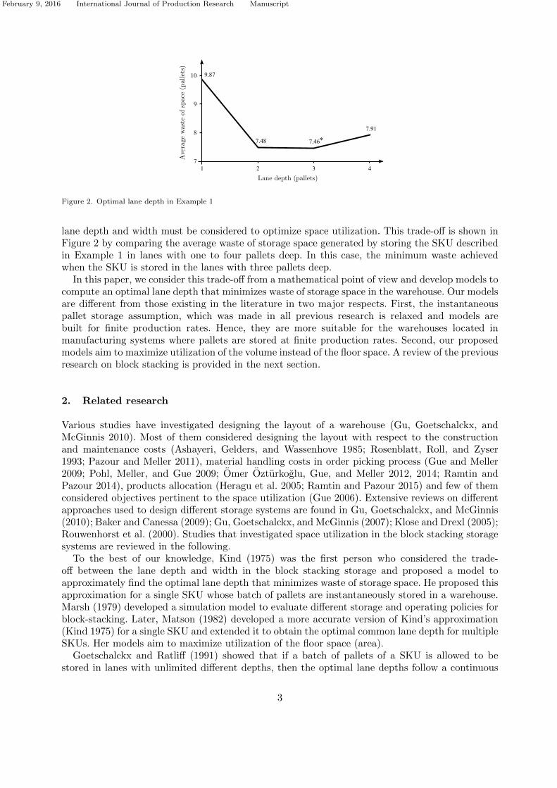
The models in this section are derived by assuming that a batch of Q pallets of a SKU is produced(or unloaded to a warehouse) at the deterministic production rate of P pallets per unit of time andblock-stacked in the lanes of x pallets deep to the height of z pallets. Pallets are depleted at thedeterministic rate of λ pallets per unit of time and aisles with a pallets width are required to accessthe lanes. Table 1 describes the notation used in the following models. The following assumptionsare made for all models in this paper:

(1) Lanes are accessible from one side and as a result, they are depleted based on last-In-first-out(LIFO).

(2) Partially occupied lanes are prioritized to be depleted first. This helps to utilize space moreefficiently because unlike the fully occupied lanes which incur only accessibility wastes to thesystem, a partially occupied lane generates both honeycombing and accessibility waste. Thus,the longer it remains incomplete, the more storage space is wasted. Another advantage of thispolicy is that these lanes are depleted faster than the fully occupied lanes and consequently,their devoted spaces are released sooner.

(3) Fully occupied lanes are depleted in an arbitrary order. This is because the order of depletingsuch lanes does not affect waste of storage space.

(4) The production, if exists, and the depletion quantities are one pallet at a time and the storage,and depletion times are assumed to be zero.

(5) No safety stock is kept in the warehouse. Production stops once all pallets of a batch areproduced and it is restarted when the inventory of the SKU becomes zero.

3.1 P = ∞, Demand is constant

In this case, pallets of SKUs are instantaneously stored in a warehouse and depleted at a finiterate. So, the production rate is considered to be infinite. Figure 4 shows the inventory level of sucha SKU over its inventory cycle time. Kind (1975) proposed the following formula to estimate theoptimal lane depth in this case:

x∗ =

√Qa

z− a

2(1)

However, he did not provide any derivation for his formula. Later, Matson (1982) developed anotherapproximation for the optimal lane depth. We derive the optimal lane depth for this case byproviding a correction on the model proposed by Matson (1982) and also considering volumeutilization instead of the floor utilization as proposed by Bartholdi (2014). The correction herein is

5


Table 1. Table of notation

P production rate (in units of pallet/time)λ depletion rate (in units of pallet/time)x lane depth (in units of pallet)x∗ optimal lane depth for single SKU (in units of pallet)x∗c optimal common lane depth for multiple SKUs (in units of pallet)z stackable height (in units of pallet)Q production (arrival) batch quantity (in units of pallet)H maximum inventory level (approximation)K maximum number of lanes required for storage (approximation)a aisle width (in units of pallets)h height of a pallet of a SKU (in units of distance i.e., inch, cm)e clear height of the warehouse (in units of pallet)n number of SKUsT inventory cycle timeOT occupied space-time in the inventory cycle timeU space utilization (single SKU)Uc space utilization for a common lane depth (multiple SKUs)WH waste of storage space caused by honeycombingWA waste of storage space dedicated to the aislesWU waste of unoccupied storage space on top of the occupied lanesW average waste of storage space (single SKU)Wc average waste of storage space for a common lane depth (multiple SKUs)

Figure 4. Changes in the inventory of a SKU stored instantaneously, P =∞

correcting the approach used to calculate total space dedicated to the aisles. However, applying thiscorrection does not change the original lane depth model proposed by Matson (1982) for the singleSKU, but the model for multiple SKUs changes as the result of optimizing volume utilization.

3.1.1 Optimal lane depth for a single SKU

The number of lanes required for storage is dQ/zxe, where dxe is the smallest integer not less thanx. Relaxing the integrality restriction, the approximate number of lanes would be

K ≈ Q

zx(2)

Assume a fully occupied lane is being depleted at the rate of λ pallets per unit of time. Once

6


the first pallet is depleted, the lane will have one unoccupied but unavailable position to the otherSKUs. This waste of storage space remains in the lane for the time period of (1/λ). Then the secondpallet is depleted and two pallet positions are wasted for the same amount of time. This waste isrendered and accumulated until the last pallet is depleted at which (zx − 1) pallet positions areunoccupied. Total pallets-time wasted in a lane as a result of honeycombing is(

1

λ

)(1 + 2 + · · ·+ (zx− 1)) (3)

Multiplying (3) by approximate number of lanes gives

WH ≈(

1

λ

)(Q(zx− 1)

2

)(4)

WA is calculated by computing total time that lanes are occupied and require accessibility.Herein, in accordance with assumption (2) in section (3), the last lane, which is most likely apartially occupied lane, is depleted first and the remaining lanes are depleted in an arbitrary order.The lane that is depleted at the last remains occupied until the whole batch is gone. So, this laneremains occupied for (1/λ)(Q) time periods. The lane depleted before this lane becomes entirelyempty (1/λ)(zx) time periods before the latter one. Thus, it remains occupied for (1/λ)(Q − zx)time periods. This process is applied to the remaining lanes, and the total time that all lanes areoccupied is (

1

λ

)(Q+ (Q− zx) + (Q− 2zx) + · · ·+ (Q−Kzx)) (5)

Each aisle is shared between two lanes located on both sides of it, so half of an aisle volume isdedicated to each lane. It is equal to (az/2) pallets. This follows that

WA ≈(

1

λ

)(Q(K + 1)−

(K(K + 1)

2

)zx

)(az2

)(6)

OT is given by

OT ≈(

1

λ

)(Q+ (Q− 1) + · · ·+ 1)

≈(

1

λ

)(Q(Q+ 1)

2

)(7)

and subsequently, space utilization is obtained by

U ≈ OTOT +WA +WH

≈ 2x(Q+ 1)

(2x+ a)(Q+ zx)(8)

Finally, the average waste of storage space is obtained by summing (4) and (6) and dividing theresult by T which is (Q/λ). That is,

W ≈(

1

4x

)(Qa− 2x+ zx(2x+ a)) (9)

7


Proposition 1. The optimal lane depth to block-stack a SKU whose batch of Q pallets is instan-taneously stored in a warehouse is

x∗ ≈√Qa

2z(10)

Proof. The optimal lane depth is obtained by taking the derivative of (9) with respect to x, set itequal to zero and solve for x.

From a practical point of view, the optimal lane depth should be an integer. To obtain aninteger lane depth, the two nearest integers to x∗ are obtained by rounding x∗ up and down andthen evaluating (9) at these values. This method can be used to obtain integer solutions for allfurther propositions.

3.1.2 Common optimal lane depth for multiple SKUs

WU needs to be computed for the multiple SKUs model. If the clear height of a warehouse in unitsof pallets of a particular SKU is denoted by e, then (e− z)x is the total pallet positions wasted ontop of a lane (stack) for the period of time that the lane is occupied by that SKU. The total timethat all lanes are occupied is given by (5). It follows that

WU ≈(

1

λ

)(Q(K + 1)−

(K(K + 1)

2

)zx

)(e− z)x (11)

Taking the clear height of the warehouse into account changes the space that a lane requires foraccessibility to (ae/2). So, expression (6) is updated accordingly.

Denote the height of a pallet of SKU i by hi. Different SKUs may have different pallet heightsand consequently be stackable to different heights. To take this into account, all waste expressionsare scaled by multiplying to a factor of hi. Total waste of storage space for each SKU is obtainedby aggregating all three types of waste. Denote the least common multiple of the inventory cycletimes of all SKUs by TLCM . Since SKUs have different inventory cycle times, Wc is determined bycalculating the total waste that all SKUs generate in TLCM and then dividing the result by TLCM .The number of inventory turns of SKU i in TLCM is TLCM (λi/Qi), and multiplying it by the totalwaste that SKU i generates in its inventory cycle time gives the total waste that SKU i generatesin the TLCM . Summing these wastes for all SKUs and dividing the result by the TLCM results inthe TLCM terms to be canceled out from the expression. Therefore from a mathematical point ofview, Wc is obtained by summing W s for all SKUs.

Wc ≈n∑i=1

(hi

4zix

)(Qiei(2x+ a) + zix(2eix+ aei − 2Qi − 2)) (12)

Uc is calculated similarly by computing the occupied and wasted space-time in TLCM . That is,

Uc ≈

∑ni=1

(λi

Qi

) (OiT)

∑ni=1

(λi

Qi

) (OiT +W i

A +W iH

)≈

2x∑n

i=1 hi(Qi + 1)

(2x+ a)∑n

i=1 eihi

(Qi

zi+ x) (13)

8


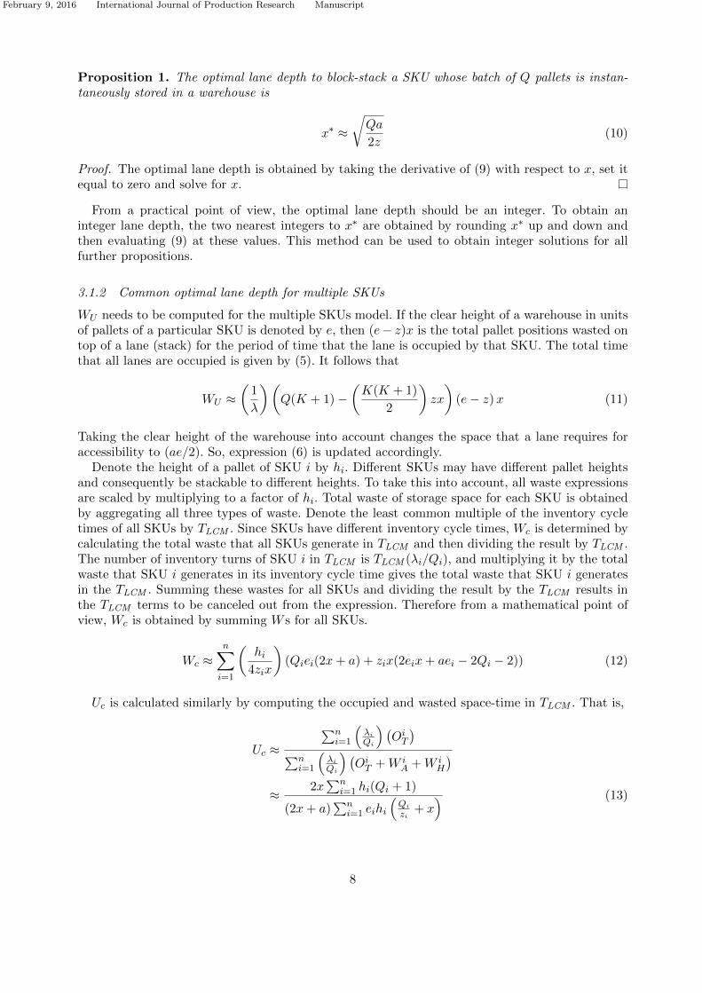
Figure 5. Changes in the inventory of a SKU stored at the rate P and depleted at the rate λ, where P > λ

where W iH , W i

A and OiT are obtained for SKU i by (4), (6) and (7), respectively. Note that TLCM

is canceled out in this expression too.

Proposition 2. The optimal common lane depth to block-stack n SKUs whose batches of palletsare instantaneously stored in a warehouse is

x∗c ≈

√√√√a∑n

i=1

(eihi

zi

)Qi

2∑n

i=1 eihi(14)

Proof. Differentiating (12) with respect to x, setting it equal to zero and solving for x gives theresult.

3.2 P > λ, demand is constant

This is a prevalent case in manufacturing systems where pallets of SKUs are produced at finiterates, stored in the warehouse and depleted at finite rates. Figure 5 shows changes in the inventorylevel of a SKU in this system. Period T1 is the production phase in which Q pallets of the SKUare produced at the rate P and stored in the warehouse. Since the demand is constant, palletsare depleted at the rate λ in this period. To simplify calculations, we assume that lanes are filledat the rate (P − λ). Production stops at the end of T1 when the inventory reaches its maximumlevel. Then, the inventory starts decreasing in T2 at the rate λ. Since the demand is constant,the inventory cycle time is (Q/λ), the maximum on-hand inventory, H, is (Q− bQλ/P c), and themaximum number of lanes required for storage is (dH/zxe) where bxc is the largest integer notgreater than x. Relaxing the integrality restriction results in the following approximations:

H ≈ Q (P − λ)

P(15)

K ≈ Q (P − λ)

Pzx(16)


WH is generated in two phases, T1 and T2. First the former is calculated. Once a pallet is stored inan empty lane, (zx− 1) pallet positions are wasted in that lane for 1/(P −λ) time periods. This is

9


the time that it takes until the next unoccupied position is filled. Then, (zx − 2) pallet positionsare wasted for the same period of time. This waste is generated and accumulated until the lastunoccupied pallet position in the lane is filled. So, the total honeycombing waste in a single lanein T1 is (

1

P − λ

)((zx− 1) + (zx− 2) + · · ·+ (zx− (zx− 1))) (17)

Multiplying (17) by K gives

WHT1≈(

(zx− 1)

2

)(Q

P

)(18)

WHT2is calculated similar to (3). Multiplying (3) by K results in

WHT2≈(zx− 1

2λ

)(Q (P − λ)

P

)(19)

WA is calculated by approximating the total time that lanes are occupied in T1 and T2. Once thefirst pallet is stored in the first lane in T1, this lane remains occupied until all (H−1) positions arefilled. Since the inventory increases at the rate (P−λ), this lane remains occupied for (H−1)/(P−λ)time periods. The second lane is used when the first one becomes fully occupied. It means (H−zx)pallet positions are remained to be filled. Once the first pallet is stored in the second lane, this laneremains occupied until the remaining (H − 1 − zx) pallet positions are filled. That is, it remainsoccupied for (H−1−zx)/(P−λ) time periods. Thus, that the total time that all lanes are occupiedin T1 is (

1

P − λ

)((H − 1) + (H − 1− zx) + (H − 1− 2zx) + · · ·+ (H −Kzx)) (20)

The total time that lanes are occupied in T2 is calculated similar to (5) but herein H pallets aredepleted, therefore Q is substituted with H in (5). Given that the dedicated aisle space to a laneis (az/2),

WA ≈((

1

P − λ+

1

λ

)(H (K + 1)− zx

(K (1 +K)

2

))− K

P − λ

)(az2

)(21)

OT is computed in T1 and T2 by

OT ≈(

1

(P − λ)

)(1 + 2 + · · ·+ (H − 1)) +

(1

λ

)(H + (H − 1) + · · ·+ 1) (22)

It follows that

U ≈ 2x(Q(P − λ) + P − 2λ)

(2x+ a)(Q(P − λ) + Pzx− 2λ)(23)

The average waste of storage space is obtained by accumulating all types of waste and dividingthe result by T , which is (Q/λ). That is,

W ≈(

1

4Px

)(2Px(zx− 1) + aP (Q+ zx)− aλ(Q+ 2)) (24)

10


Figure 6. Space utilization vs. average waste of storage space

Figure 6 compares space utilization and the average waste of storage space with respect to lanedepth. At x∗, the space utilization and the average waste of storage space reach their maximumand minimum values, respectively.

Proposition 3. The optimal lane depth to block-stack a SKU whose batch of pallets is producedat the rate P and depleted at the rate λ, where P > λ, is

x∗ ≈√a (Q(P − λ)− 2λ)

2zP(25)

Proof. It is proved by taking the derivative of (24) with respect to x, setting it equal to zero andsolving for x.


WU is calculated by multiplying the total time that lanes are occupied in T1 and T2 by the unoccu-pied volume on top of lanes which is (e− z)x pallets. WA is computed similar to (21), except thatthe aisle space that a lane requires for accessibility changes to (ae/2). Scaling all waste expressionsby multiplying them by hi, summing them, and dividing the result by T results in W for SKU i.Wc is obtained by aggregating the W s for all SKUs. That is,

Wc ≈n∑i=1

(hi

4Pizix

)(Pi(Qiei(2x+ a) + zix(2eix− 2Qi + aei − 2))− λ(Qi + 2)(2x(ei − zi) + aei))

(26)Uc is obtained as described in (13). That is,

Uc ≈2x∑n

i=1

(hi

Pi

)(Qi(Pi − λi)− 2λi + Pi)

(2x+ a)∑n

i=1 eihi(x+(

1Pizi

)(Qi(Pi − λi)− 2λi))

(27)

Proposition 4. The optimal common lane depth to block-stack n SKUs whose batches of palletsare produced at the rate P and depleted at the rate λ, where P > λ, is

x∗c ≈

√√√√a∑n

i=1

(eihi

ziPi

)(Qi(Pi − λi)− 2λi)

2∑n

i=1 eihi(28)

11


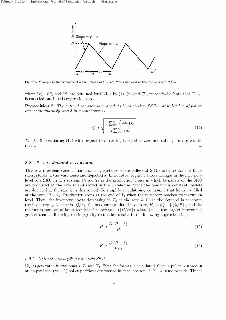
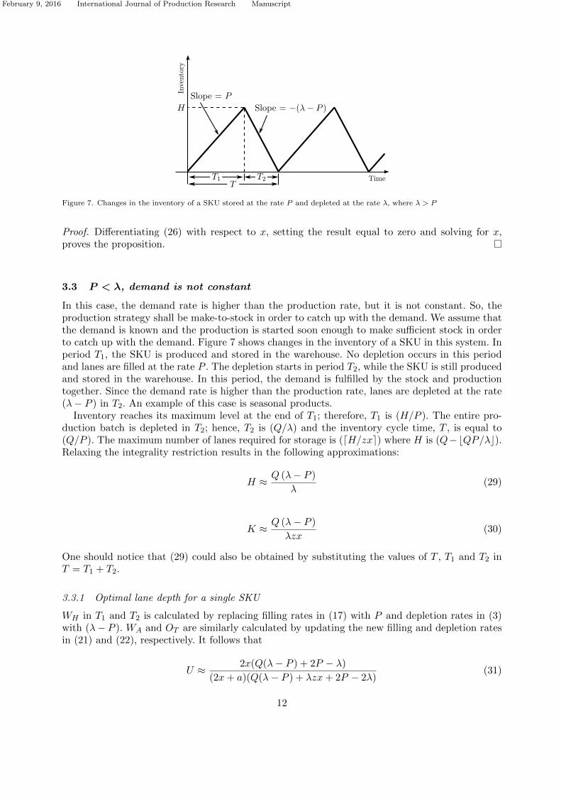
Figure 7. Changes in the inventory of a SKU stored at the rate P and depleted at the rate λ, where λ > P

Proof. Differentiating (26) with respect to x, setting the result equal to zero and solving for x,proves the proposition.

3.3 P < λ, demand is not constant

In this case, the demand rate is higher than the production rate, but it is not constant. So, theproduction strategy shall be make-to-stock in order to catch up with the demand. We assume thatthe demand is known and the production is started soon enough to make sufficient stock in orderto catch up with the demand. Figure 7 shows changes in the inventory of a SKU in this system. Inperiod T1, the SKU is produced and stored in the warehouse. No depletion occurs in this periodand lanes are filled at the rate P . The depletion starts in period T2, while the SKU is still producedand stored in the warehouse. In this period, the demand is fulfilled by the stock and productiontogether. Since the demand rate is higher than the production rate, lanes are depleted at the rate(λ− P ) in T2. An example of this case is seasonal products.

Inventory reaches its maximum level at the end of T1; therefore, T1 is (H/P ). The entire pro-duction batch is depleted in T2; hence, T2 is (Q/λ) and the inventory cycle time, T , is equal to(Q/P ). The maximum number of lanes required for storage is (dH/zxe) where H is (Q−bQP/λc).Relaxing the integrality restriction results in the following approximations:

H ≈ Q (λ− P )

λ(29)

K ≈ Q (λ− P )

λzx(30)

One should notice that (29) could also be obtained by substituting the values of T , T1 and T2 inT = T1 + T2.


WH in T1 and T2 is calculated by replacing filling rates in (17) with P and depletion rates in (3)with (λ− P ). WA and OT are similarly calculated by updating the new filling and depletion ratesin (21) and (22), respectively. It follows that

U ≈ 2x(Q(λ− P ) + 2P − λ)

(2x+ a)(Q(λ− P ) + λzx+ 2P − 2λ)(31)

12


W is determined by summing all types of waste and then dividing the result by T , which is(Q/P ). That is,

W ≈(

1

4λx

)(2λx(zx− 1) + aλ(Q+ zx− 2)− aP (Q− 2)) (32)

Proposition 5. The optimal lane depth to block-stack a SKU whose batch of pallets is producedat the rate P and depleted at the rate λ, where P < λ, is

x∗ ≈√a(Q− 2)(λ− P )

2zλ(33)

Proof. It is proven by taking the derivative of (32) with respect to x, setting it equal to zero andsolving for x.


WU is calculated as described in section (3.2.2) using the new filling and depletion rates. WA iscomputed as described for the single SKU model. Herein, the aisle space that a lane requires foraccessibility changes to (ez/2). To take the pallet heights into account, all waste expressions arescaled by multiplying by hi. Summing the W s for all SKUs results in the average waste of storagespace for a common lane depth.

Wc ≈n∑i=1

(hi

4λizix

)(λi(ei(Qi − 2)(2x+ a) + zix(2eix+ aei − 2Qi + 2))− Pi(Qi − 2)(2x(ei − zi) + aei))

(34)It follows that

Uc ≈2x∑n

i=1

(hi

λi

)(Qi(λi − Pi) + 2Pi − λi)

(2x+ a)∑n

i=1 eihi(x+(

1λizi

)(Qi(λi − Pi) + 2Pi − 2λi))

(35)

Proposition 6. The optimal common lane depth to block-stack n SKUs whose batches of palletsare produced at the rate P and depleted at the rate λ, where P < λ, is

x∗c ≈

√√√√a∑n

i=1

(eihi

ziλi

)(Qi − 2)(λi − Pi)

2∑n

i=1 eihi(36)

Proof. Differentiating (34) with respect to x, setting the result equal to zero and solving for x,proves it.

4. Experimental framework

The experimental framework is designed as follows: First, we describe the simulation model usedto evaluate performance of the proposed models. Next, the test problem sets are described andthen accuracy of the proposed models is evaluated by the simulation model. Finally, the finite andinfinite production rate models are compared with respect to the optimal lane depth and spaceutilization.

13


Algorithm 1 Pseudo-code of the simulation

Initialize parameters (Pi, λi, Qi, zi, x, a, n)Schedule first events for all SKUswhile (simulation time not terminated) do

Find the earliest eventif (the event is production (arrival)) then

if (a partially occupied lane is available for the SKU) thenAssign the SKU to the lane

elseDedicate a new lane to the SKU

elseif (a partially occupied lane is available for the SKU) then

Deplete the SKU from the laneelse

Deplete the SKU from a fully occupied lane

Update the lane occupanciesUpdate WH , WA, WU and OTSchedule the next event for the SKU

return Wc and Uc

Table 2. Parameters of the triangular distributions used in the simulation

Variables Low Mode High

Production time 1P (1− 0.3) 1

P1P (1 + 0.3)

Demand inter-arrival time 1λ(1− 0.5) 1

λ1λ(1 + 0.5)

Batch size Q(1− 0.3) Q Q(1 + 0.3)

4.1 Simulation model

The pseudo-code of the simulation model used for evaluation (an event-oriented model writtenin Python) is shown in Algorithm 1. The main goal of the experimental analysis is to evaluateaccuracy of the proposed models for the real world situations where stochastic variations existamong the major production factors and demand. For this reason, the simulation model utilizesrandom variables for the production times, demand inter-arrival times, and the batch sizes aspresented in Table 2.

To compute the performance metrics under the stochastic variations, the simulation model isrun for lane depths from 5 to 50 pallets deep and replicated 40 times for each lane depth. Theaverage waste of storage space is computed for each replication and the average of results withinthe replications is recorded for each lane depth. Finally the lane depth that generated the minimumaverage waste of space is reported as the optimal lane depth. Common random numbers were usedfor all lane depths in the same replication to ensure that randomness does not interfere in selectingthe optimal lane depth. However, the number of replications must be determined such that theconfidence intervals on the average waste of space obtained for any two consecutive lane depthsdo not overlap. Our experiments showed that 40 replications sufficiently narrows the confidenceintervals such that this condition is met. Also, they showed that the space utilization convergesfaster when the warm-up period is set to 10 percent of the simulation period.

Our objective is to evaluate the long time performance of the system, therefore the simulationperiod must be defined long enough to cover sufficient numbers of inventory cycles for each SKU inthe test problems. Considering the randomly generated test problems, the inventory cycle times in

14


Table 3. Parameters of the uniform distributions used to generate the random SKUs

VariablesP > λ P < λ

Min Max Min Max

P (pallet/hour) λ 100 0.5 10λ (pallet/hour) 0.1 2 P 15z (pallet) 2 5 2 5a (pallet) 2 4 2 4h (feet) 2 5 2 5Pallet cost 50$ 500$ 50$ 500$

our test problems vary from less than a month to higher than 6 months. Thus, we set the simulationperiod to five years for both single and the multiple SKU test problems.

4.2 Analyzing accuracy of the models

The performance of the models was analyzed on randomly generated test problems for single andmultiple SKUs. The test problems were designed as described in the following:

• Single SKU: A repository of 1000 SKUs were randomly generated for each of the two finiteproduction rate models. Uniform random distributions with the parameters shown in Table3 were used to generate the SKUs. The following are the non-random parameters used ingenerating the SKUs:◦ monthly holding cost: (pallet cost)×0.3/12◦ setup cost: (pallet cost)×5◦ warehouse clear height: 25 feet◦ Q: computed by the EOQ model (Nahmias 2005)The SKU repository for the infinite production rate model was created by duplicating the

SKU repository generated for the finite production rate with P > λ and discarding the λs.The simulation model was run for the 1000 SKUs in each repository one by one and the

results were compared with the outputs of the relevant models.• Multiple SKUs: For each of the three cases investigated in this paper, three test sets

were designed for 10, 50 and 100 SKU test problems. Each test set consists of 30 differenttest problems whose SKUs were randomly chosen from the relevant SKU repository. For allmultiple SKU test problems, aisle width was set to three pallets.

The accuracy of the proposed models in estimating the optimal lane depth and space utilizationwas evaluated by calculating the Mean Absolute Percentage Error (MAPE) between the modelestimations and the simulation results. The MAPE for the optimal lane depth is calculated as

MAPEx∗ =1

N

N∑i=1

∣∣xSi − x∗i ∣∣xSi

(37)

where xSi and x∗i are the optimal lane depth obtained by the simulation and the proposed modelsfor the ith test problem, respectively, and N is the number of the test problems, which is equal to1000 and 30 for the single and multiple SKU test sets, respectively. The MAPE for space utilization

15


Figure 8. The MAPE for the optimal lane depth and space utilization, P =∞

Figure 9. The MAPE for the optimal lane depth and space utilization, P > λ

Figure 10. The MAPE for the optimal lane depth and space utilization, P < λ

is obtained by

MAPEU =1

(N × 45)

N∑i=1

50∑j=5

∣∣∣USij − Uij∣∣∣USij

(38)

where USij is the average space utilization within the 40 replications of simulation for the lanedepth j in test problem i and Uij is the space utilization estimated by the relevant model for thelane depth j in test problem i. Figures 8, 9 and 10 show the MAPEx∗ and MAPEU for the threeinvestigated cases. The following observations are obtained from the experimental study:

16


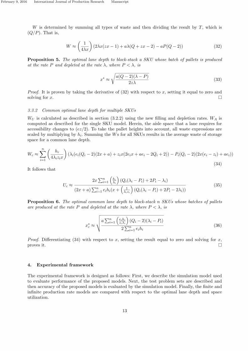
Figure 11. The MAPE for the space utilization estimated by the finite and infinite production rate models

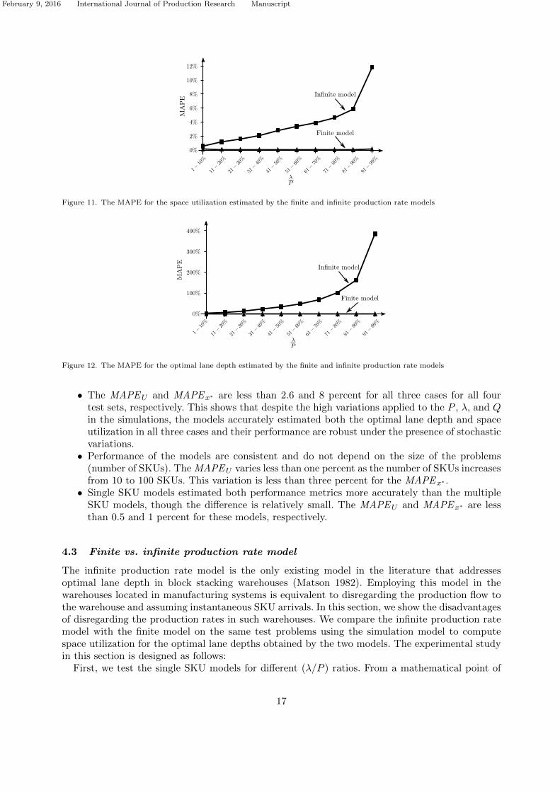
Figure 12. The MAPE for the optimal lane depth estimated by the finite and infinite production rate models

• The MAPEU and MAPEx∗ are less than 2.6 and 8 percent for all three cases for all fourtest sets, respectively. This shows that despite the high variations applied to the P , λ, and Qin the simulations, the models accurately estimated both the optimal lane depth and spaceutilization in all three cases and their performance are robust under the presence of stochasticvariations.• Performance of the models are consistent and do not depend on the size of the problems

(number of SKUs). The MAPEU varies less than one percent as the number of SKUs increasesfrom 10 to 100 SKUs. This variation is less than three percent for the MAPEx∗ .• Single SKU models estimated both performance metrics more accurately than the multiple

SKU models, though the difference is relatively small. The MAPEU and MAPEx∗ are lessthan 0.5 and 1 percent for these models, respectively.

4.3 Finite vs. infinite production rate model

The infinite production rate model is the only existing model in the literature that addressesoptimal lane depth in block stacking warehouses (Matson 1982). Employing this model in thewarehouses located in manufacturing systems is equivalent to disregarding the production flow tothe warehouse and assuming instantaneous SKU arrivals. In this section, we show the disadvantagesof disregarding the production rates in such warehouses. We compare the infinite production ratemodel with the finite model on the same test problems using the simulation model to computespace utilization for the optimal lane depths obtained by the two models. The experimental studyin this section is designed as follows:

First, we test the single SKU models for different (λ/P ) ratios. From a mathematical point of

17


Table 4. Finite vs. infinite production rate models

Metric10 SKUs 50 SKUs 100 SKUs

Min Max Avg. Min Max Avg. Min Max Avg.

Improvement finite modelachieved in space utilization

0.36% 3.67% 2.09% 0.87% 3.25% 1.94% 0.76% 2.68% 1.86%

Optimal lane depth (finitemodel)

14 21 17.8 15 19 17.60 16 19 17.43

Optimal lane depth (infinitemodel)

24 40 30.00 26 34 29.90 26 33 29.63

view, the infinite production rate model is a special case of the finite model where P > λ. Thatis, (10) can be alternatively obtained by substituting( P = ∞) in (25). This experiment aims todetermine when the infinite model is capable of estimating optimal lane depth for a finite productionrate problem with a relatively small error. Then, performance of both models are examined formultiple SKUs with respect to space utilization. Single and multiple SKU test problems are designedfor this experiment as described in the following:

• Single SKU: 10 different test problems each consisting of 1000 randomly generated SKUswere generated similar to the SKU repositories in section 4.2 except that here, the demandrates were generated such that the (λ/P ) ratios for all SKUs in the first, second, ..., andthe tenth test problems were in the ranges 1-10 percent, 11-20 percent,..., 91-99 percent,respectively.• Multiple SKUs: Two SKU repositories were randomly generated as described in section

4.2. Herein, the demand rates were generated such that (λ/P ) ratios were between 5 to 30percent for the SKUs in the first repository and between 70 to 95 percent for the ones inthe second repository. Then, three test sets were designed each containing 30 test problemsfor 10, 50 and 100 SKUs, respectively. For each test problem, 70 percent of its SKUs wererandomly chosen from the first SKU repository and the remaining were randomly chosenfrom the second repository. This setup aims to preserve diversity among the SKUs in the testproblems.

Figure 11 and 12 compare the MAPEU and MAPEx∗ for the single SKU models for different(λ/P ) ratios. The infinite production rate model obtained relatively small errors when the ratio isless than 10 percent. As the ratio increases, both the MAPEU and the MAPEx∗ drastically increasefor the infinite model. On the contrary, the finite model obtained relatively small and consistenterrors for all ranges.

Table 4 shows the test results for the multiple SKU test problems. On average, the optimal lanedepths obtained by the finite production rate model resulted in about two percent higher spaceutilization than the ones obtained by the infinite model. This improvement is almost consistentamong the three test sets. On the other hand, the infinite model obtained much deeper lanes thanthe finite model. The average of the optimal lane depths estimated by the infinite model is morethan 68 percent deeper than the average of the ones obtained by the finite model. Deep lanes forma warehouse layout that has few cross aisles and therefore, the transportation costs increase inthe warehouse. So, the layout designed by the finite model is more flexible and also incurs lesstransportation costs. However, quantifying this cost is out of the scope of this paper and is an openproblem for a future research.

The optimal lane depths obtained by the finite model achieved higher space utilization in alltest problems. This improvement increases when the production rates are closer to the demandrates, like just-in-time manufacturing systems where the production lines are in balance with thedemand.

18


5. Conclusion

In this paper, we developed mathematical models to obtain the optimal lane depth for single andmultiple SKUs in block stacking storage systems under finite production rate constraints. The fol-lowing cases were studied: infinite production rate, finite production rate where the production rateis higher than the demand rate, and less than the demand rate. A simulation model was developedto evaluate performance of the models for the real word situation where uncertainty exists in pro-duction and demand. That is, the assumptions of constant, deterministic production and demandwere relaxed in the simulation. An experimental study was carried out on the randomly generatedtest problems for single and multiple SKUs. The experimental analysis shows that although themodels were developed based on the assumption of deterministic production and demand, they arerobust and accurate under uncertainty.

We evaluated the finite production rate model with the only existing model in the literature (in-finite production rate model) on the same test problems and highlighted the advantages achievedin the space utilization and transportation costs by taking the production rates into considera-tion. The optimal lane depth obtained by the finite model led to higher space utilization in alltest problems. They are nearly half as deep as the ones obtained by the infinite production ratemodel. This implies, they form a flexible layout that contains more cross aisles and as a result lesstransportation costs are incurred to the system.

Our proposed models accurately estimate the lane depth that enhances space utilization in blockstacking warehouses in manufacturing systems. However, it is important to note that our modeldoes not consider safety stock or transportation costs which could influence the results in practice.Considering both space utilization and Transportation costs in finding the optimal lane depthseems a substantial problem for future research.

References

Ashayeri, J., L. Gelders, and L. Van Wassenhove. 1985. “A microcomputer-based optimization model forthe design of automated warehouses.” International Journal of Production Research 23 (4): 825–839.

Baker, Peter, and Marco Canessa. 2009. “Warehouse design: A structured approach.” European Journal ofOperational Research 193 (2): 425 – 436.

Bartholdi, John J. 2014. “A note on the most space-effcient lane-depth for block-stacked pallets.” PrivateNote .

Carlo, Hctor J., Iris F.A. Vis, and Kees Jan Roodbergen. 2014. “Storage yard operations in containerterminals: Literature overview, trends, and research directions.” European Journal of Operational Research235 (2): 412 – 430.

Goetschalckx, Marc, and H. Donald Ratldff. 1991. “Optimal lane depths for single and multiple productsin block stacking storage systems.” IIE Transactions 23 (3): 245–258.

Gu, Jinxiang, Marc Goetschalckx, and Leon F. McGinnis. 2007. “Research on warehouse operation: Acomprehensive review.” European Journal of Operational Research 177 (1): 1 – 21.

Gu, Jinxiang, Marc Goetschalckx, and Leon F. McGinnis. 2010. “Research on warehouse design and per-formance evaluation: A comprehensive review.” European Journal of Operational Research 203 (3): 539 –549.

Gue, Kevin R. 2006. “Very high density storage systems.” IIE Transactions 38 (1): 79–90.Gue, Kevin R., Elif Akcali, Alan Erera, Bill Ferrell, and Gary Forger. 2014. “The U.S. Roadmap for Material

Handling & Logistics.” .Gue, Kevin R., and Russell D. Meller. 2009. “Aisle configurations for unit-load warehouses.” IIE Transactions

41 (3): 171–182.Heragu, S. S., L. Du, R. J. Mantel, and P. C. Schuur. 2005. “Mathematical model for warehouse design and

product allocation.” International Journal of Production Research 43 (2): 327–338.Hudock, Brian. 1998. “Warehouse space and layout planning.” In The warehouse management handbook,

edited by James A Tompkins and Jerry D Smith, 2nd ed. Tompkins press.

19


Jang, Dong-Won, Se Won Kim, and Kap Hwan Kim. 2013. “The optimization of mixed block stackingrequiring relocations.” International Journal of Production Economics 143 (2): 256 – 262.

Kind, DA. 1975. “Elements of space utilization.” Transportation and Distribution Management 15: 29–34.Klose, Andreas, and Andreas Drexl. 2005. “Facility location models for distribution system design.” European

Journal of Operational Research 162 (1): 4 – 29.Larson, T.Nick, Heather March, and Andrew Kusiak. 1997. “A heuristic approach to warehouse layout with

class-based storage.” IIE Transactions 29 (4): 337–348.Marsh, WH. 1979. “Elements of block storage design.” International Journal of Production Research 17 (4):

377–394.Matson, J. O. 1982. “The analysis of selected unit load storage systems.” Ph.D. thesis, Georgia Institute of

Technology, Atlanta, GA.Nahmias, Steven. 2005. Production & operations analysis. 5th ed. McGraw-Hill.Omer Ozturkoglu, Kevin R. Gue, and Russell D. Meller. 2012. “Optimal unit-load warehouse designs for

single-command operations.” IIE Transactions 44 (6): 459–475.Omer Ozturkoglu, Kevin R. Gue, and Russel D. Meller. 2014. “A constructive aisle design model for unit-

load warehouses with multiple pickup and deposit points.” European Journal of Operational Research 236(1): 382 – 394.

Pazour, Jennifer A., and Russell D. Meller. 2011. “An analytical model for A-frame system design.” IIETransactions 43 (10): 739–752.

Petering, Matthew E.H., and Mazen I. Hussein. 2013. “A new mixed integer program and extended look-ahead heuristic algorithm for the block relocation problem.” European Journal of Operational Research231 (1): 120 – 130.

Pohl, Letitia M., Russell D. Meller, and Kevin R. Gue. 2009. “Optimizing fishbone aisles for dual-commandoperations in a warehouse.” Naval Research Logistics 56 (5): 389–403.

Ramtin, Faraz, and Jennifer A. Pazour. 2014. “Analytical models for an automated storage and retrievalsystem with multiple in-the-aisle pick positions.” IIE Transactions 46 (9): 968–986.

Ramtin, Faraz, and Jennifer A. Pazour. 2015. “Product allocation problem for an AS/RS with multiplein-the-aisle pick positions.” IIE Transactions 47 (12): 1379–1396.

Rosenblatt, Meir J., Yaakov Roll, and D Vered Zyser. 1993. “A combined optimization and simulationapproach for designing automated storage/retrieval systems.” IIE Transactions 25 (1): 40–50.

Rouwenhorst, B., B. Reuter, V. Stockrahm, G.J. van Houtum, R.J. Mantel, and W.H.M. Zijm. 2000. “Ware-house design and control: Framework and literature review.” European Journal of Operational Research122 (3): 515 – 533.

Van den Berg, Jeroenp. 1999. “A literature survey on planning and control of warehousing systems.” IIETransactions 31 (8): 751–762.

Yang, JeeHyun, and KapHwan Kim. 2006. “A grouped storage method for minimizing relocations in blockstacking systems.” Journal of Intelligent Manufacturing 17 (4): 453–463.

20

Documents

Optimizing Space Utilization in Block Stacking Warehouses · PDF file2/9/2016 · stacking warehouse where the objectives are maximizing space utilization and minimizing trans-portation