Optimizing Supply Chain Conﬁguration Considering Supply

121

Innovation and Supply Chain Management, Vol. 8, No. 3, pp. 121–133, September 2014

Optimizing Supply Chain Configuration Considering Supply Disruption

Ruiqing XIA 1, Tang LIU 1, and Hiroaki MATSUKAWA 1

1 Department of Administration, Faculty of Science and Technology, Keio University, Japan

Abstract : The purpose of this paper is to investigate a supplier-retailer supply chain that experiences disruptions insupplier during the planning horizon. There are multiple options to supply a raw material, to manufacture or assemble theproduct, and to transport the product to the customer. While determine what suppliers, parts, processes, and transportationmodes to select at each stage in the supply chain, options disruption must be considered. In this paper, we show thatchanges to the original plan induced by a disruption may impose considerable deviation costs throughout the system.When the production plan and the supply chain coordination scheme are designed in a static manner, as is most oftenthe case, both will have to be adjusted under a disruption scenario. Using dynamic policies, we derive conditions underwhich the supply chain can be coordinated so that the maximum potential profit is realized.

Key Words : Supply chain disruptions management, Scenario planning, Business continuity management, Supply dis-ruption, Supply chain configuration, Dynamic Programming

1. Introduction

In 1905, ‘The Independent’ newspaper uses the word ”SupplyChain” in the news article about wartime situation, which is thefirst use of the word “Supply Chain”. A supply chain is theapplication of processes and tools to ensure the optimal opera-tion of a manufacturing and distribution supply chain. Supplychain activities transform natural resources, raw materials, andcomponents into a finished product that is delivered to the endcustomer. It takes a while for people to realize a supply chaincan be managed and optimized. To make the supply chain moreoptimal and flexible to utilize, a concept is introduced. In 1982,the term “supply chain management” first entered public do-main. Supply chain management (SCM) is the management ofthe flow of goods. It includes the movement and storage of rawmaterials, work-in-process inventory, and finished goods frompoint of origin to point of consumption. Interconnected or in-terlinked networks, channels and node businesses are involvedin the provision of products and services required by end cus-tomers in a supply chain. To be more specific, it includes theoptimal placement (including safety stock) of inventory withinthe supply chain and minimizing operating costs. When wetalk about and try to function the SCM, the mathematical mod-eling techniques are often involved. Most of these models arestrategic in the sense that they optimize both safety stock lev-els and safety stock holding locations across the supply chain.There has been significant advancement in the safety stock opti-mization strategies in the last few decades. There are two mainreasons for this. First, the past decades has seen a diffusionof supply chain knowledge throughout the organization. Thisdiffusion of knowledge enables companies and managers to an-alyze and model supply chain. Second, more advanced tools

Corresponding Author: Ruiqing XiaDepartment of Administration Engineering, Keio University([email protected])(Received July 5, 2014)(Revised August 7, 2014)(Accepted September 3, 2014)

including computer software are made that business users canuse to actually perform the analysis.

1.1 Supply Chain NetworkWhat is a supply chain network? And why are they so importantfor logistics and business managers? Supply chain networks al-low us to look at the big picture; giving us a better understand-ing of the flow of materials and information.

Often organizations focus only on their organization; whatthey produce or provide and not what the end customer re-ceives. Looking at a supply chain network enables firms to lookat the overall movement of materials/information from start toend, allowing organizations to see the value in creating part-nerships; and the value in working together to ensure the bestpossible value is provided to the end-customer.

Supply chain networks describes the flow and movement ofmaterials & information, by linking organizations together toserve the end-customer.

Network describes a more complex structure, where orga-nizations can be cross-linked and there are two-way exchangesbetween them; chain describes a simpler, sequential set of links.

A supply chain network shows the links between organiza-tions and how information and materials flow between theselinks. The more detailed the supply chain network the morecomplex and web like the network becomes. And to get a com-plete picture of an organizations supply chain network; infor-mation & material flow should be mapped. Inefficiency canthen be located and removed.

• Material flow: Is the movement of goods from raw pri-mary goods (such as Wool, Trees and Coal etc.) to com-plete goods (TVs, Radios and Computers) that are to bedelivered to the final customer

• Information flow: Is the demand from the end-customer topreceding organizations in the network.

If a focal firm provides their suppliers with their sales data/forecasting demand information; their supplier will be able to

Innovation and Supply Chain Management, DOI: http://dx.doi.org/10.14327/iscm.8.121 , Copyrightc⃝ ISCM Forum 2014 all rights reserved

Innovation and Supply Chain Management, Vol. 8, No. 3, September 2014122

reduces costs (such as over production waste) and improveprices. In order to better serve end customers it is important todevelop strong partnerships within your supply network whichhas a flow on effect to your end customers whether you are amanufacturer, distributor or retailer. Better communication willincrease efficiency and productivity. Trust is the core ingredientto developing better communication and relationships. We willtalk about this topic based on our assumption afterwards.

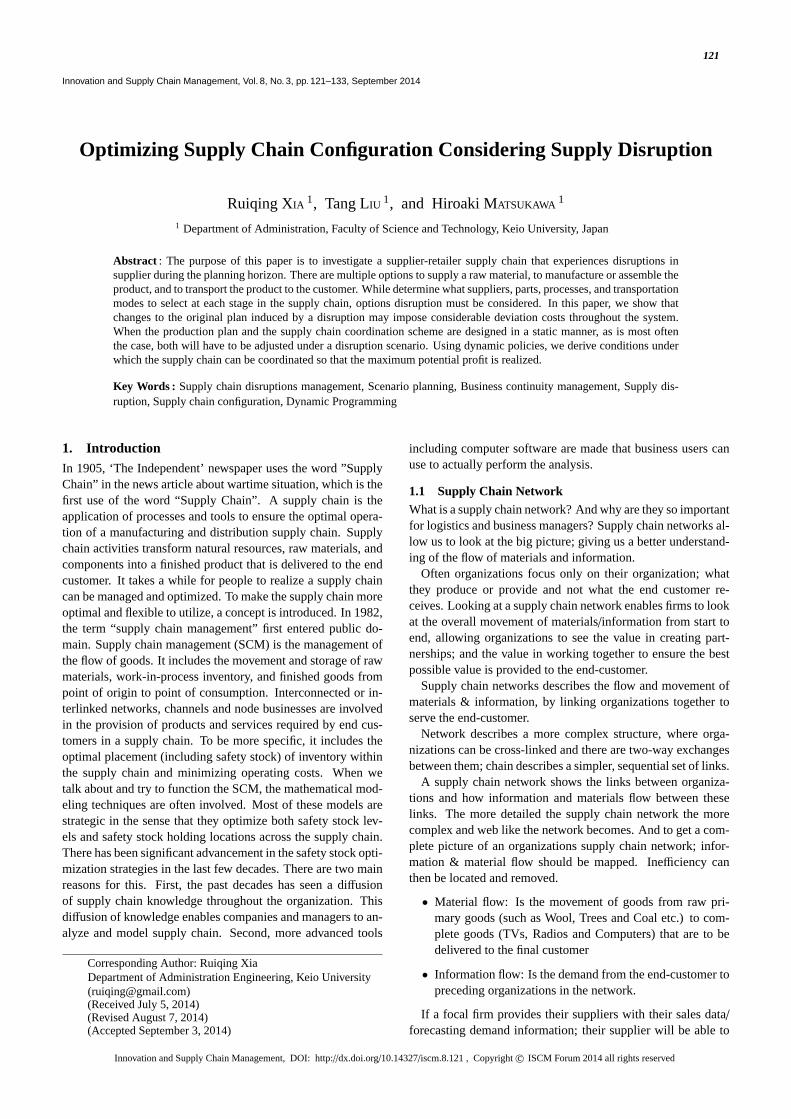
Fig. 1 Apple juice organization network

1.2 Demand Planning and Sales Forecasting

When we talk about SCM, it always comes as the problem suchas who is responsible for forecasting the needs of the supplychain? Where does demand/usage begin? These are just twoquestions supply chain professionals might ask when focusingon the end user or consumer.

Without shared and readily available information on end usersales and demands, all other trading partners and those withina company not directly related to end user demand are workingoff “derived demand” from supply chain individual enterprisesales.

Within each echelon, several forecasts are alive but oftenwithout the consensus of all parties in a company, much lessthe entire supply chain. A company develops business forecastsand goals, as well as product/market forecasts, to achieve broadlong-term financial development benchmarks. These forecastsprovide a basis for resource planning, which ultimately leadsto shorter-term, monthly forecasts aimed at deriving the “num-bers” that drive earnings for the year.

Sales and operations planning next addresses resource load-ing to meet two to six month plans for capacity use and supplyplanning. Finally, short-term production forecasts are neededto set production, operations, and sales schedules.

For most businesses, a key question is whether they have con-sensus for forecasts to drive the company. Forecasts are oftenbased on different assumptions and metrics dollars, units, andshipments, for example.

Extend this thinking to supply chain forecasting among trad-ing partners, and a similar question arises. Is there consensus-based communication among trading partners? Often, forecastsand schedules are not shared, leading to the bullwhip effect thatDr. Jay Forrester and his MIT colleagues first discussed in thelate 1950’s.

1.3 Sourcing Strategy

With the development of supply chain management and mod-els, there are much more aspects of the chain that the companiesand managers and business users need to concern. Among themare the single or dual sourcing and supply disruptions.

When setting up an inventory policy, first of all it has to bedecided whether to source all of the replenishment from onesupplier, or to divide the orders among dual sources. To dualsource means to use two preferred suppliers to provide the sameproduct or service. To single source means to use just one pre-ferred supplier, despite there being multiple capable suppliersavailable. Both single sourcing and dual sourcing have theirown advantages and disadvantages. The selection of suppliersheavily depends on the purchase price and the lead time char-acteristics of the suppliers. Often the choices are made eitherfor an expensive and flexible (for example choices with shortlead time) suppliers or cheap but rigid suppliers. Yet, it maybe profitable to use two suppliers. Many purchasers decide tosingle or dual source based on certain assumptions.

1.4 Supply Disruption

Supply disruptions may be caused by diverse reasons includ-ing nature disasters, equipment failures or damaged facilities,during which a supplier cannot fulfil customer orders and theninfluence flows of the whole supply chain (Chen,H.Zhao andX.Zhao, 2012[4]). Supply chain disruption has been proven tohave seriously negative impact on corporate profitability andshareholder value. In order to cope with uncertainty in inven-tory systems, buffers are held to protect service performanceagainst unforeseen events. If distribution takes place at variousstages, the problem becomes more complex because of addi-tional opportunity of allocating buffers to the stage of the sys-tems.

Every supply chain faces disruptions of various sorts. Re-cent examples of major disruptions are easy to bring to mind:Hurricanes Katrina and Rita in 2005 on the U.S. Gulf Coastcrippled the nations oil refining capacity, destroyed large in-ventories of coffee and lumber, and forced the rerouteing ofbananas and other fresh produce. A strike at two General Mo-tors parts plants in 1998 led to the shut-downs of 26 assemblyplants, which ultimately resulted in a production loss of over500,000 vehicles and an 809 million quarterly loss for the com-pany. An eight-minute fire at a Philips semiconductor plantin 2001 brought one customer, Ericsson, to a virtual stand-still while another, Nokia, weathered the disruption. Moreover,smaller-scale disruptions occur much more frequently. For ex-ample, Wal-Marts Emergency Operations Center receives a callvirtually every day from a store or other facility with some sortof crisis .There is evidence that superior contingency planningcan significantly mitigate the effect of a disruption. For ex-ample, Home Depots policy of planning for various types ofdisruptions based on geography helped it get 23 of its 33 storeswithin Katrinas impact zone open after one day and 29 afterone week, and Wal-Marts stock prepositioning helped make ita model for post-hurricane recovery. Similarly, Nokia weath-ered the 2001 Phillips fire through superior planning and quickresponse, ultimately allowing it to capture a substantial portionof Ericsson’s market share.

Innovation and Supply Chain Management, Vol. 8, No. 3, September 2014 123

2. Literature Reviews

Numerous papers address optimizing inventory and safety stockplacement across the supply chain. Lin et al. (2000) andBillington et al. (2004) both present examples where multi-echelon inventory theory was successfully distributed to a largeset of business users within a company. In the work summa-rized in Billington et al. (2004), multiechelon inventory theoryoptimization tools have been transferred to more than 100 busi-ness users within Hewlett Packard, producing savings in excessof $150 million. But all those theories are derived from variouspapers from the past.

There are some approaches to safety stock placement. One ofthem is stochastic-service model approach. Lee and Billington(1993) develop a multi-echelon inventory model to reflect thedecentralized supply chain structure they witnessed in HewlettParkard’s DeskJet printer supply chain. Their goal was to pro-duce a model that manufacturing and materials managers coulduse to evaluate different strategic decisions involved with thecreation of a new-product supply chain. They model a supplychain as a collection of locations where each stage in the sup-ply chain accepts as an exogenous input a service level targetor a base stock policy. In the case where service level targetswere inputs, the authors develop a single-stage base-stock cal-culation that, while approximate, is tractable. The single-stagebase-stock level is a function of the replenishment lead-timeas the stages, which includes the production lead-time. Leeand Billington show how to propagate the single-stage modelto multiple stages. Ettl, Feigin, Lin and Yao (2000) also con-sider a supply chain context that is quite similar in spirit to thework of Lee and Billington (1993). The single-stage base-stockmodel in Ettl et al. (2000) makes a distinction between thenominal lead-time a stage quotes and the actual lead-time thestage experiences. The actual lead-time will exceed the nomi-nal lead-time when there is a stock-out at a supplier. Glasser-man and Tayur (1995) consider a context very similar to thatof Lee and Billington (1993) and Ettl et al.(2000) but go on tointroduce capacity limits into their multi-echelon model. Theproblem formulation of Glasserman and Tayur (1995) followsthe framework of Clark and Scarf (1960) with the addition ofcapacity.

The guaranteed service-time approach traces its lineage backto the 1955 manuscript, which was later reprinted in 1988(Kim-ball,1988). In that paper, Kimball describes the mechanics ofs single stage that operated a base-stock policy in the face ofrandom but bounded demand. In particular, beyond the deter-ministic production time assumed at the stage, there is an in-coming service time that represents the delivery time quotedfrom the stage’s supplier and an outgoing service time repre-senting the delivery time the stage quotes to bounded. Simp-son (1958) determined optimal safety stocks for a supply chainmodelled as a serial network by using Kimball’s work as thebuilding block, coupling adjacent stages together through theuse of service time. This topic is based on similar assumptionabout the demand process and internal control policies for thesupply chain.

Our work is related to Simpson (1958), and is also relatedto that of Inderfurth (1991,1993), who also build off Simpsonsframework for optimizing safety stocks in a supply chain. In-derfurth(1993) considers the optimization of safety stock costs

and lead times for a single production process production mul-tiple end items. The optimization captures the impact that thefinished goods lead time have on the safety stock in the sup-ply chain and the procedure for valuation of these effects thatis presented in his paper can be applied to general multi-stageproduction systems with convergent or divergent structure andcan be used as a helpful tool for assessing the cost/service per-formance of investments in reducing length and variability oflead-time in complex production systems. However, the modelonly considers changing the configuration at one stage in thesupply chain and only considers safety stock costs. Also, ourwork is related to Ettl et al. (2000), which examines the de-termination of the optimal base-stock levels in a supply chain,and tries to do so in a way that is applicable to practice. Ettlet al. (2000) also develops performance evaluation models of amulti-stage inventory system, where the key challenge is howto approximate the replenishment lead-time within the supplychain. They then formulate and solve a non-linear optimizationproblem that minimizes the supply chain inventory costs sub-ject to user-specified requirement on the customer service level.Because the models from Ettl et al. and its cited papers con-sider existing supply chains, there is already one option chosenat each stage. Therefore, the cost of goods sold (COGS) is set,as is the holding cost of the pipeline inventory, and these costsdo not enter into the analysis. Geoffrion and Powers (1995) de-scribe the evolution in the network design field which focuseson developing the optimal manufacturing and distribution net-work for a company’s entire product line. Network design fo-cuses more on the two or more echelons in the supply chain formultiple products the supply chain configuration problem focuson a single product family at the supply chain level, allowing itto model all the echelons in the supply chain and to explicitlycapture the impact of variability on the supply chain.

Graves and Willems(2000a) and Graves and Willems(2005)address the optimizing safety stock placement across the sup-ply chain. The work of Graves and Willems (2000a) is similarin that we also assume base-stock policies and focus on mini-mizing the inventory requirements in a supply chain. The re-sulting models and algorithms are much different, though, dueto different assumption about the demand process and differentconstraints on service levels within the supply chain.

The objective of our paper differs from the existing single-echelon and multi echelon models with multiple suppliers intwo respects. First, we are not trying to model an optimal re-plenishment policy at an operational level of detail. We rathertake a more strategic view and focus on the placement of safetystock across the network. Based on the empirical evidence pro-vided in the introduction and for reasons of analytical tractabil-ity, we assume that a static allocation of the demand shall beassigned to each supplier in every period at a strategic planninglevel. The static allocation is treated as exogenous based onlong-run time averages and company-specific policies, such asminimum production quantities for facilities.

Second, we consider larger networks with multiple suppli-ers and multiple echelons. To this end, we build on the Gravesapproach for multi echelon inventory optimization, which hasbeen shown to be applicable to supply networks of larger sizes.So far, all the model of Graves and Willems contributions as-sume that each item is sourced from a single supplier.

Therefore, in this paper, we investigate an supplier-retailer


supply chain that in which the suppliers may have the probabil-ity of disruptions during the planning horizon. The model underinvestigation is mostly related to Graves and Willems(2005).Yet, more aspects are concerned based on the origin model.Soley, Graves and Willems (2005) briefly outline an approxi-mate approach of how to incorporate multiple suppliers in thefinal section of their paper. We extend the Graves and Willems(2005) model to dual sourcing strategy and also the disruptionrisk is added.

The goals of this research are therefore:

• To extend and compare the single and dual sourcing.

• To analyse in both cases the effects of a suppliers disrup-tion.

• To compare the model with some existed solutions relatedto supply chain

All those goals are applied to a multi-stage supply chain witha configuration optimization problematic.

The structure of this paper is shown as follow. In chapter3, we introduce the assumptions. The model is formulates inchapter 4 and in chapter 5 we will show the dynamic program-ming method we use to solve the problem. Numerical cases areprovided in chapter 5 and we conclude the paper in chapter 6.

3. Supply Chain Configuration3.1 Multi-stage Network

We model a supply chain as a network where nodes, stages andarcs are included. Arcs denote that an upstream stage suppliesa downstream stage. A stage can represent a major processingfunction in the supply chain. A stage might represent the pro-curement of a raw material, or the production of a component,or the manufacture of a sub-assembly, or the assembly and testof a finished good, or the transportation of a finished productfrom a central distribution center to a regional warehouse. Eachstage is a potential location for holding a safety-stock inventoryof the item processed at the stage. Nodes denote the options forthe stage. An option at a stage is characterized by its lead timeand added cost.

We assume that if a stage is connected to several upstreamstages, then its production activity is an assembly requiring in-puts from each of the upstream stages. A stage that is connectedto multiple downstream stages is either a distribution node ora production activity that produces a common component formultiple internal customers.

3.2 Production Lead-Time

For each stage, we assume a known deterministic productionlead time. When a stage reorders, the lead time is the time fromwhen all of the inputs are available until production is com-pleted and available to serve demand. The production lead timeincludes the waiting and processing time at the stage, plus anytransportation time to put the item into inventory. For example,if stagek requires inputs from stagei and j, then for a produc-tion request made at timet, stagek completes the production attime t+Tk, Tk represents the lead time of stagek, provided thatthere are adequate supplies ofi and j at timet.

We assume that the lead time is not impacted by the size ofthe order; hence, we assume that there are no capacity con-straints that limit production at a stage.

3.3 Inventory Policy

We assume that all stages operate with a periodic review base-stock replenishment policy with a common review period. Foreach period, each stage observes demand either from an exter-nal customer or from its downstream stage, and places orderson its suppliers to replenish the observed demand. No time de-lay in ordering need to be concerned, hence, in each period theordering policy passes the external customer demand back upthe supply chain so that all stages see the customer demand.

3.4 Demand Process

We assume that external demand occurs only at nodes that haveno successors, which we term demand nodes or stages.

For each demand nodej, we assume that the end-item de-mand comes from a stationary process for which the averagedemand per period isu j . Because an internal stage has only in-ternal customers or successors; its demand at time t is the sumof the orders placed by its immediate successors. Since eachstage orders according to a base-stock policy, the demand atinternal stagei is di(t) =

∑(i, j)∈A d j(t)

whered j(t) denotes the realized demand at stagej in periodt and A is the arc set for the network representation of the sup-ply chain. For every arc (i, j) belongs to A, stagej orders anamountd j(t) from upstream stagei in time periodt. The aver-age demand rate for stagei is µi =

∑(i, j)∈A µ j

We assume that demand at each stagei is bounded by a max-imum demand functionDi(t). We haveD j(τ) ≥ d j(t − τ + 1)+d j(t − τ + 2) + ... + d j(t) We defineD j(0)=0 and assume thatD j(t) is increasing and concave.

We presume that it is possible to establish a meaningful up-per bound on demand over varying horizons for each end item,which means in the context of setting safety stocks: the safetystock is set to cover all demand realizations that fall withinthe upper bounds. If demand exceeds the upper bounds, thenthe safety stock will not be adequate by design. Given suchcase, the manager resorts to other tactics to handle the exceeddemand. A manager indicates explicitly a preference for howdemand variation should be handled what range is covered bysafety stock and what range is handled by other actions or re-sponses.

As an example, consider a typical assumption where demandfor end item j is normally distributed each period andi.i.d.,where meanµ and standard deviationσ. Therefore, a man-ager might specify the demand bounds at the demand node byD j(τ) = τµ + kσ

√τ wherek represents the percentage of time

that the safety stock covers the demand variation. The choiceof k indicates how frequently the manager is willing to resortto other tactics to cover demand variability. For the rest of thepaper, we will defineD as shown above.

3.5 Guaranteed Service Time

We assume that each demand nodej promises a guaranteed ser-vice timeSout

j . Which means, the customer demand at timet,the demand at stagej in periodt, d j(t), must be filled by timet + Sout

j . We do not explicitly model a trade-off between pos-sible shortage costs and the costs for holding inventory. how-ever, when we have asked the managers for their desired servicelevel, we have found that managers seem more comfortablewith the notion of 100% service for some range of demand; theyaccept the fact that if demand exceeds this range, they will have


shortages unless they can somehow expand the response capa-bility of their supply chain.(Graves and Willems,2000) There-fore, We assume that stagej provides 100% service for thespecified service time: stagej delivers exactlyd j(t) to the cus-tomer at timet + Sout

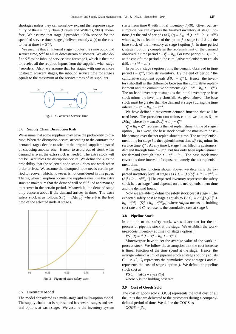
j .We assume that an internal stagei quotes the same outbound

service time,Souti to all its downstream customers. We also de-

fineSini as the inbound service time for stagei, which is the time

to receive all the required inputs from the suppliers when stagei reorders. Also, we assume that for stages with one or moreupstream adjacent stages, the inbound service time for stageiequals to the maximum of the service times of its suppliers.

Fig. 2 Guaranteed Service Time

3.6 Supply Chain Disruption Risk

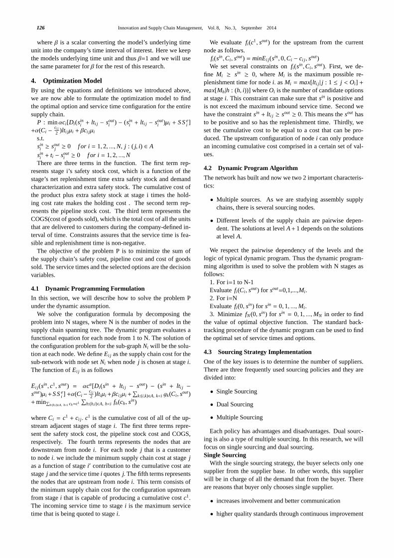
We assume that some suppliers may have the probability to dis-rupt. When the disruption occurs, according to the contract, thedemand stages decide to stick to the original suppliers insteadof choosing another one. Hence, to avoid out of stock whendemand arrives, the extra stock is needed. The extra stock willnot be used unless the disruption occurs. We define theρi as theprobability that the selected node stagei does not work whenorder arrives. We assume the disrupted node needs certain pe-riod to recover, which, however, is not considered in this paper.That is, when disruption occurs, the suppliers must use the extrastock to make sure that the demand will be fulfilled and manageto recover in the certain period. Meanwhile, the demand stageonly concern about if the demand arrives in time. The extrasafety stock is as followsS Se

i = Di(ti)ρ2i whereti is the lead

time of the selected node at stagei.

Fig. 3 Figure of extra safety stock

3.7 Inventory Model

The model considered is a multi-stage and multi-option model.The supply chain that is represented has several stages and sev-eral options at each stage. We assume the inventory system

starts from time 0 with initial inventoryI i j (0). Given our as-sumption, we can express the finished inventory at stagei op-tions j at the end of periodt asI i j (t) = Si j−di(t−sin

i −lt i j , t−souti )

wherelt i j is the lead time of the optionj at stagei andSi j is thebase stock of the inventory at stagei option j. In time periodt, stagei option j completes the replenishment of the demandobserved in time periodt− sin

i − lt i j , For time periodt− si − lt i j ,at the end of time periodt, the cumulative replenishment equalsdi(0, t − sout

i − lt i j )In periodt, stagei option j fills the demand observed in time

period t − souti , from its inventory. By the end of periodt the

cumulative shipment equalsd(i 0, t − sout

i ). Hence, the inven-tory shortfall is the difference between the cumulative replen-ishment and the cumulative shipmentsdi(t − sin

i − lt i j , t − souti ).

The on-hand inventory at stagei is the initial inventory or basestock minus the inventory shortfall. As given above. The basestock must be greater than the demand at stagei during the timeintervalt − sin

i − lt i j , t − souti .

We have defined a maximum demand function that will beused here. The precedent constraints can be written asSi j =

Di(ti j ) whereti j = max0, sini + lt i j − sout

t

sini + lt i j − sout

t represents the net replenishment time of stageioption j. In a word, the base stock equals the maximum possi-ble demand over the net replenishment time. The net replenish-ment time for stagei is the replenishment timesin

i +lt i j minus itsservice timesout

i . At any timet, stagei has filled its customers’demand through timet − sout

i , but has only been replenishmentfor demand through timet − sin

t − lt i j . The base stock mustcover this time interval of exposure, namely the net replenish-ment time.

By using the function shown above, we determine the ex-pected inventory level at stage i asEIi = [Di(Sin

i + lt i j − souti ) −

(Sini + lt i j − sout

i )µi ] The expected inventory represents the safetystock held at stagei, and depends on the net replenishment timeand the demand bound.

Now we are able to define the safety stock cost at stagei. Theexpected safety cost at stagei equals toESCi = αCi [Di(Sin

i +

lt i j − souti )− (Sin

i + lt i j − souti )µi ] where/alphameans the holding

cost rate andCi represents the cumulative cost at stagei.

3.8 Pipeline Stock

In addition to the safety stock, we will account for the in-process or pipeline stock at the stage. We establish the work-in-process inventory at timet of stagei option j.

PSi j (t) = di(t − sini − lt i j , t − sout

i )Moreover,we have to set the average value of the work-in-

process stock. We follow the assumption that the cost increaseis linear function of the time spend at the stage. Hence, theaverage value of a unit of pipeline stock at stage i option j equalsCi − ci j/2, Ci represents the cumulative cost at stagei andci j

represents the cost of stagei option j. We define the pipelinestock cost as

PSC= [α(Ci − ci j/2)lt i j ]whereα is the holding cost rate.

3.9 Cost of Goods Sold

The cost of goods sold (COGS) represents the total cost of allthe units that are delivered to the customers during a company-defined period of time. We define the COGS as

COGS= βci j


whereβ is a scalar converting the model’s underlying timeunit into the company’s time interval of interest. Here we keepthe models underlying time unit and thusβ=1 and we will usethe same parameter forβ for the rest of this research.

4. Optimization ModelBy using the equations and definitions we introduced above,we are now able to formulate the optimization model to findthe optimal option and service time configuration for the entiresupply chain.

P : minαci [Di(sini + lt i j − sout

i ) − (sini + lt i j − sout

i )µi + S Sei ]

+α(Ci − ci j

2 )lt i jµi + βci jµi

s.t.sini ≥ sout

j ≥ 0 f or i = 1,2, ...,N, j : ( j, i) ∈ A

sini + ti − sout

i ≥ 0 f or i = 1,2, ...,NThere are three terms in the function. The first term rep-

resents stage i’s safety stock cost, which is a function of thestage’s net replenishment time extra safety stock and demandcharacterization and extra safety stock. The cumulative cost ofthe product plus extra safety stock at stage i times the hold-ing cost rate makes the holding cost . The second term rep-resents the pipeline stock cost. The third term represents theCOGS(cost of goods sold), which is the total cost of all the unitsthat are delivered to customers during the company-defined in-terval of time. Constraints assures that the service time is fea-sible and replenishment time is non-negative.

The objective of the problem P is to minimize the sum ofthe supply chain’s safety cost, pipeline cost and cost of goodssold. The service times and the selected options are the decisionvariables.

4.1 Dynamic Programming Formulation

In this section, we will describe how to solve the problem Punder the dynamic assumption.

We solve the configuration formula by decomposing theproblem into N stages, where N is the number of nodes in thesupply chain spanning tree. The dynamic program evaluates afunctional equation for each node from 1 to N. The solution ofthe configuration problem for the sub-graphNi will be the solu-tion at each node. We defineEi j as the supply chain cost for thesub-network with node setNi when nodej is chosen at stagei.The function ofEi j is as follows

Ei j (sin, c1, sout) = αca[Di(sin + lt i j − sout) − (sin + lt i j −sout)µi +S Se

i ] +α(Ci − ci j

2 )lt iµi +βci jµi +∑

k:(i,k)∈A, k<i gk(Ci , sout)+min∑

h:(h,i)∈A, h<i ch=c1∑

h:(h,i)∈A, h<i fh(ch, sin)

whereCi = c1 + ci j . c1 is the cumulative cost of all of the up-stream adjacent stages of stagei. The first three terms repre-sent the safety stock cost, the pipeline stock cost and COGS,respectively. The fourth terms represents the nodes that aredownstream from nodei. For each nodej that is a customerto nodei. we include the minimum supply chain cost at stagejas a function of stagei′ contribution to the cumulative cost atestagej and the service timei quotesj. The fifth terms representsthe nodes that are upstream from nodei. This term consists ofthe minimum supply chain cost for the configuration upstreamfrom stagei that is capable of producing a cumulative costc1.

The incoming service time to stagei is the maximum servicetime that is being quoted to stagei.

We evaluatefi(c1, sout) for the upstream from the currentnode as follows.

fi(sin,Ci , sout) = minEi j (sin,0,Ci − ci j , sout)We set several constraints onfi(sin,Ci , sout). First, we de-

fine Mi ≥ sin ≥ 0, whereMi is the maximum possible re-plenishment time for nodei. asMi = max[lt i j | j : 1 ≤ j < Oi ] +max[Mh|h : (h, i))] whereOi is the number of candidate optionsat stagei. This constraint can make sure thatsin is positive andis not exceed the maximum inbound service time. Second wehave the constraintsin + lt i j ≥ sout ≥ 0. This means thesout hasto be positive and so has the replenishment time. Thirdly, weset the cumulative cost to be equal to a cost that can be pro-duced. The upstream configuration of nodei can only producean incoming cumulative cost comprised in a certain set of val-ues.

4.2 Dynamic Program Algorithm

The network has built and now we two 2 important characteris-tics:

• Multiple sources. As we are studying assembly supplychains, there is several sourcing nodes.

• Different levels of the supply chain are pairwise depen-dent. The solutions at levelA+ 1 depends on the solutionsat levelA.

We respect the pairwise dependency of the levels and thelogic of typical dynamic program. Thus the dynamic program-ming algorithm is used to solve the problem with N stages asfollows:

1. For i=1 to N-1Evaluatefi(Ci , sout) for sout=0,1,...,Mi .2. For i=NEvaluatefi(0, sin) for sin = 0,1, ...,Mi .3. Minimize fN(0, sin) for sin = 0,1, ...,MN in order to find

the value of optimal objective function. The standard back-tracking procedure of the dynamic program can be used to findthe optimal set of service times and options.

4.3 Sourcing Strategy Implementation

One of the key issues is to determine the number of suppliers.There are three frequently used sourcing policies and they aredivided into:

• Single Sourcing

• Dual Sourcing

• Multiple Sourcing

Each policy has advantages and disadvantages. Dual sourc-ing is also a type of multiple sourcing. In this research, we willfocus on single sourcing and dual sourcing.Single Sourcing

With the single sourcing strategy, the buyer selects only onesupplier from the supplier base. In other words, this supplierwill be in charge of all the demand that from the buyer. Thereare reasons that buyer only chooses single supplier.

• increases involvement and better communication

• higher quality standards through continuous improvement


• better pricing through higher volumes

• build stronger and longer-term relationship

• single sources are typically open to negotiations. Thesevendors need business and they are often willing to ac-commodate business owners and modify contract terms inorder to stay a step ahead of their competition

Even though single sourcing has some benefits, it also hasweakness. Putting all the requirement on one supplier alsomeans risky. The risk of production disruption for the buyercan be high in case of supply difficulties. For example. in 2000,Philips, the microchip supplier for Ericsson, suffered a fire sothat it was disable to produce and provide any chip to Ericssonfor a few weeks. This factory was the only supplier of Ericsson.As we can expect that this accident had dramatic consequenceson Ericsson at least $400 million in potential revenue lost. An-other issue is that single sourcing is less flexibility as the sup-plier has a limited production capacity. Finally the purchaseproduct might not be the cheapest because of the loyalty to thesupplier and the potentially existing supplier changing costs.

[t]Dual Sourcing

By using dual sourcing policy, the buyer or the business de-cider chooses two suppliers, one of which may dominate theother in terms of business, share, price, reliability, etc. In theevent of disruption, such as the Thailand floods of 2011, thecompany envisions with the possible loss of one supplier, thesecond supplier could ramp up production to offset and mini-mize production disruption. However, normally applying dualsourcing will cost more than single sourcing and another issuewith dual sourcing as well as multiple sourcing is to determinethe procurement quantities to each supplier. Table 4.1 showsthe benefits of the single sourcing and dual sourcing.Sourcing Splitting Ratio

With dual sourcing policy, we have to set the sourcing ra-tio between the selected suppliers. There are various strategiesavailable. We can choose either 50%-50% splitting or a strategythat a dominant supplier providing the main part of the neces-sary supply and a second supplier providing the rest. Therefore,we will follow the 80%-20% splitting. This ratio is set by Mr.Vilfredo Pareto, hence it is also called The Pareto Principle,which states that roughly 80% of the effects come from 20% ofthe causes. For example in business 80% of the sales come from20% of the clients. This ratio is widely used in both businessand industry area.Select the Second Option of the Dual Sourcing

After choosing the best option at each node, we have tochoose the second option in order to use dual sourcing. A fewdecision strategies are available here.

One would be choosing the second option at each node withthe configuration program. That is, we first run the programnormally. We obtain as solution the best options at each stageto minimize the total supply chain cost. As we want to findthe second best options at each node, we erase the best optionsfrom the set of all available options. We return the configura-tion program. Therefore, as we removed the best options, weobtain the second best options for minimizing the total supplychain cost. In this case, we do not have to change the logicalpart of the program based on our definition in previous sections.

We only need to run the program twice to get the results. How-ever, this method can not guarantee that the solution of the totalsupply chain is the overall most optimized options. Cost of firstbest options plus the cost of second best options does not meanit is most optimal for logical reasons.

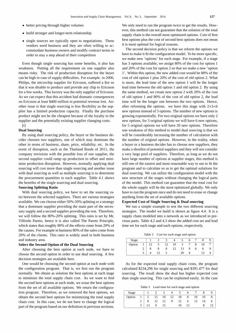
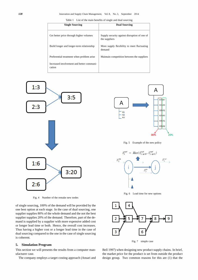
The second decision policy is that we reform the options wehave to make it fit the configuration model. To be more specific,we make new ’options’ for each stage. For example, if a stagehas 3 options available, we assign 80% of the cost for option 1and 20% of the cost for option 2 so that we make a new ’option1’. Within this option, the new added cost would be 80% of thecost of old option 1 plus 20% of the cost of old option 2. Whatis more, the lead time of the new option 1 will be the longerlead time between the old option 1 and old option 2. By usingthe same method, we create new option 2 with 20% of the costof old option 1 and 80% of the cost of old option 2, the leadtime will be the longer one between the two options. Hence,after reforming the options. we have this stage with 2×3=6new options instead of 3 options. The number of new options isgrowing exponentially. For two original options we have only 2new options, for 3 original options we will have 6 new options,for 5 original options we will have 20 new options. Thereforeone weakness of this method to model dual sourcing is that wewill be considerably increasing the number of calculation withthe number of original options. However, in the reality, whena buyer or a business decider has to choose new suppliers, theymake a shortlist of potential suppliers and they will not considera very large pool of suppliers. Therefore, as long as we do nothave large number of options at supplier stages, this method isstill one of the easiest and most reasonable way to use to fit theprogram and to calculate so as to get the optimal solutions fordual sourcing. We can utilize the configuration model with thenew structure of the stages without changing the logical partsof the model. This method can guarantee that the total cost forthe whole supply will be the most optimized globally. We onlyhave to run the program once and do not need to erase or changeanything from the set of available options.Expected Cost of Single Sourcing & Dual sourcing

We run a simple example to test the two different sourcingstrategies. The model we build is shown as figure 4.4. It is asupply chain modeled into a network as we introduced in pre-vious parts. Table 4.2 and 4.3 show the added cost set and leadtime set for each stage and each options, respectively.

Table 2 Cost for each stage and option

Stage 1 2 3 4 5 6 7 8 9Option 1 12 5 12 10 3 7 8 10 7

2 8 8 8 12 13 9 6 6 93 4 12 5 20 4 12 4

As for the expected total supply chain costs, the programcalculated $234,296 for single sourcing and $391.477 for dualsourcing. The result show the dual has higher expected costthan single sourcing. This can be explained easily. In the case

Table 3 Lead time for each stage and option

Stage 1 2 3 4 5 6 7 8 9Option 1 5 15 10 12 18 8 10 10 8

2 8 12 12 9 12 6 12 14 63 13 9 15 10 12 8 12


Table 1 List of the main benefits of single and dual sourcing

Single Sourcing Dual Sourcing

Get better price through higher volumes Supply security against disruption of one ofthe suppliers

Build longer and longer-term relationship More supply flexibility to meet fluctuatingdemand

Preferential treatment when problem arise Maintain competition between the suppliers

Increased involvement and better communi-cation

Fig. 4 Number of the remake new nodes

of single sourcing, 100% of the demand will be provided by theone best option at each stage. In the case of dual sourcing, onesupplier supplies 80% of the whole demand and the not the bestsupplier supplies 20% of the demand. Therefore, part of the de-mand is supplied by a supplier with more expensive added costor longer lead time or both. Hence, the overall cost increases.Thus having a higher cost or a longer lead time in the case ofdual sourcing compared to the one in the case of single sourcingis coherent.

5. Simulation Program

This section we will presents the results from a computer man-ufacturer case.

The company employs a target costing approach (Ansari and

Fig. 5 Example of the new policy

Fig. 6 Lead time for new options

Fig. 7 simple case

Bell 1997) when designing new product supply chains. In brief,the market price for the product is set from outside the productdesign group. Two common reasons for this are (1) that the


product faces many competitors and the firm will be a pricetaker and (2) that another department within the company, forexample, marketing, specifies the product’s selling price. Next,a gross margin for the product is specified, typically by seniormanagement or corporate finance. The combination of the pre-specified selling price and the gross margin target dictates theproducts maximum unit cost. The product’s unit manufactur-ing cost (UMC) is the sum of the direct costs for the productionof a single unit of product. Typical costs include raw materi-als, the processing cost at each stage, and transportation. Themaximum unit cost acts as an overall budget for the product’sUMC.

From an organizational perspective, the supply chain devel-opment core team is composed of an early supply chain en-abler and one or two representatives associated with each of theproduct’s major sub-assemblies. The early supply chain enableris responsible for shepherding the product through the productdevelopment process. This individual is brought in during theearly design phase and will stay with the project until it achievesvolume production.

The core team will allocate the UMC budget across the majorsub-assemblies. This is not an arbitrary process. The team willrely on a number of factors, including competitive analysis, pastproduct history, future cost estimates, and value engineering.Once the sub-assembly budgets are set, the design teams foreach sub-assembly are charged with producing a sub-assemblythat can provide the functionality required subject to its budgetconstraint. Even if these groups incorporate multidisciplinaryteams and concurrent engineering, they will still operate withintheir own budget constraints.

In much the same way that the UMC is allocated to the sub-assemblies, each sub-assembly group allocates its budget anddecides what processes and components to use. There are nu-merous factors to consider when sourcing a component, someof which include functionality, price, vendor delivery history,vendor quality, and vendor flexibility. Because many of thesefactors are difficult to quantify, the team establishes a minimumthreshold for each of the intangible factors. Suppliers that meetor exceed the thresholds are considered as candidates or op-tions.

The company’s current practice is essentially to choose thelowest unit cost option from the set of options that satisfy theintangible factors. In the framework of the supply chain config-uration problem, this corresponds to choosing the options withthe lowest cost added at each stage, regardless of its lead time.While this is admittedly a heuristic, there are several reasonsthe company does this. First, as mentioned earlier, all other fac-tors besides cost are difficult, if not impossible, to quantify. Forexample, the company only wants to do business with suppliersthat have been certified. The certification process involves a rig-orous review of the supplier’s quality practices, but given twocertified suppliers, there is no mechanism to view one supplier’squality as superior to the other. Second, the UMC of the productwill dictate whether the business case to launch the product issuccessful. If the UMC were not low enough to meet the grossmargin target, then the project will be terminated. Therefore,there is tremendous pressure to focus on the UMC at the ex-pense of other considerations. Finally, the team that designs thesupply chain is not the same team that has to manage the supplychain. Although choosing parts with long lead times might sig-

nificantly increase the supply chain’s inventory requirements,this dynamic has not been explicitly considered during the newproduct’s business case analysis.

5.1 Notebook Computer Case Study

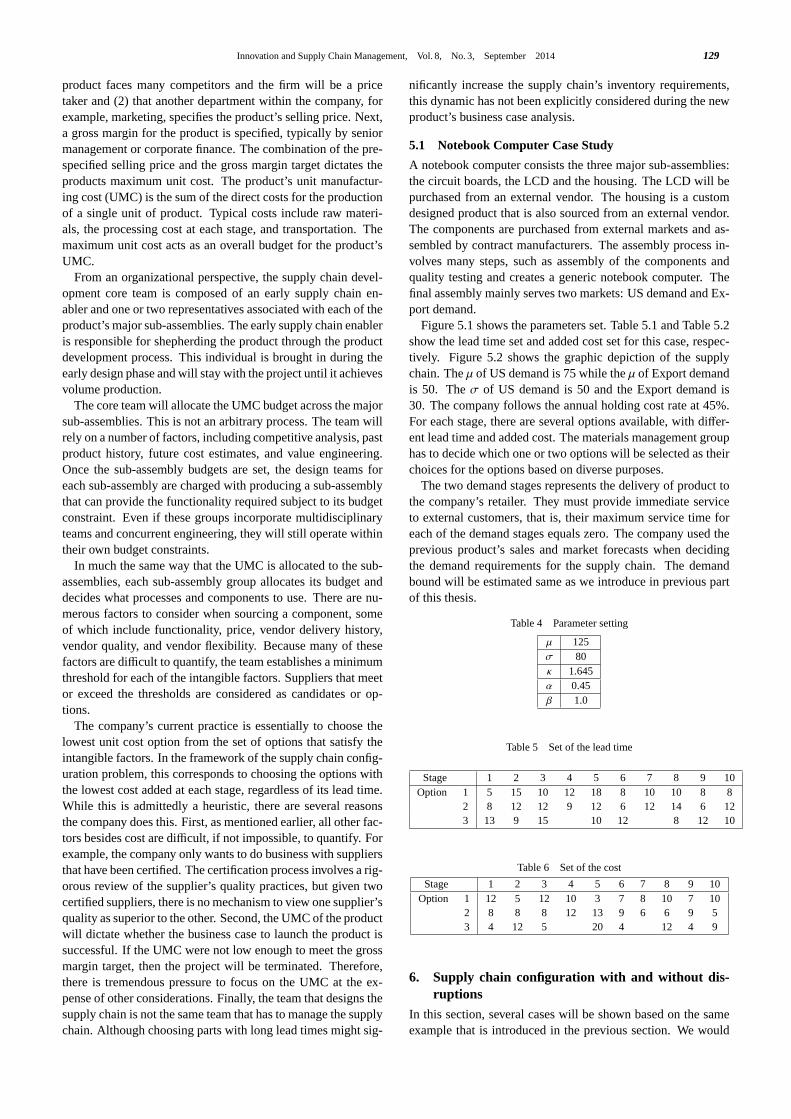
A notebook computer consists the three major sub-assemblies:the circuit boards, the LCD and the housing. The LCD will bepurchased from an external vendor. The housing is a customdesigned product that is also sourced from an external vendor.The components are purchased from external markets and as-sembled by contract manufacturers. The assembly process in-volves many steps, such as assembly of the components andquality testing and creates a generic notebook computer. Thefinal assembly mainly serves two markets: US demand and Ex-port demand.

Figure 5.1 shows the parameters set. Table 5.1 and Table 5.2show the lead time set and added cost set for this case, respec-tively. Figure 5.2 shows the graphic depiction of the supplychain. Theµ of US demand is 75 while theµ of Export demandis 50. Theσ of US demand is 50 and the Export demand is30. The company follows the annual holding cost rate at 45%.For each stage, there are several options available, with differ-ent lead time and added cost. The materials management grouphas to decide which one or two options will be selected as theirchoices for the options based on diverse purposes.

The two demand stages represents the delivery of product tothe company’s retailer. They must provide immediate serviceto external customers, that is, their maximum service time foreach of the demand stages equals zero. The company used theprevious product’s sales and market forecasts when decidingthe demand requirements for the supply chain. The demandbound will be estimated same as we introduce in previous partof this thesis.

Table 4 Parameter setting

µ 125σ 80κ 1.645α 0.45β 1.0

Table 5 Set of the lead time

Stage 1 2 3 4 5 6 7 8 9 10Option 1 5 15 10 12 18 8 10 10 8 8

2 8 12 12 9 12 6 12 14 6 123 13 9 15 10 12 8 12 10

Table 6 Set of the cost

Stage 1 2 3 4 5 6 7 8 9 10Option 1 12 5 12 10 3 7 8 10 7 10

2 8 8 8 12 13 9 6 6 9 53 4 12 5 20 4 12 4 9

6. Supply chain configuration with and without dis-ruptions

In this section, several cases will be shown based on the sameexample that is introduced in the previous section. We would


Fig. 8 Notebook case structure

like to consider the supply chain configuration when the dis-ruptions happen. We assume that the disruptions may happenat any stage, we will calculate the numerical case by setting adisruption probability.

Some solutions are available for the disruption case. First isthat for all the stages that have probability to disruption, noneof them keeps the extra safety stock. When the disruption hap-pens, all the disrupted suppliers will be abandoned instantly andthe buyer or the business decider will choose another supplierthat works well at the same stage. Second is that for all thestages that have probability to disruption, each of them holdsextra safety stock, once the disruption happens, the buyer willnot change the suppliers and all the disrupted suppliers willmeet the demand from the customers by using the extra safetystock, and we assume that all the disrupted suppliers will re-covery in on unit time.

We first do the simulation for the case in which all the dis-rupted suppliers will be abandoned right after the disruptionshappens. We set 5% disruption probability for stage 5. Whichmeans, in the supply chain, there is 95% probability that thewhole chain will work without troubles and 5% probability thatthe the best optimal option, which is responsible for 80% ofthe whole demand from its customer at stage LCD have to bechanged.

We define the expected supply chain cost for this assumptionshown as

[ECdi j ] = (1− ρi j )Ei + (ρi j )Ed

i j whereρi j means the disruptionprobability at stagei option j, Ei j means the whole supply chaincost without disruption at stagei option jandEd

i j represents thethe supply chain cost with disruption.

Table 5.3 shows the new optimal solutions that after the dis-rupted supplier is changed, the optimal options of the supplychain using dual sourcing strategy. The total cost for this as-sumption is $437,418. This increases the cost of no disruptionsupply chain by 0.8%.

Notice that in the above case we assume that any suppli-ers that are under disruption will be abandoned. However, inthe real world, the demand stage may not be able to changethe suppliers in a short period. The suppliers must have extrasafety stock to meet the demand in case the disruption happens.Therefore, under this condition, we have another result with thesame nodes option as shown in figure 3 but a different total costwhich equals to 453,008. This increases the cost of no disrup-tion concerned by 4.32% and increases the cost of the abovecase by 3.56%.

From the comparisons we know that it might be optimal ifthe buyer change the suppliers instantly when disruption hap-pens. But in the real world scenario, sometimes changing thesuppliers may cost more than expect because there are always

Table 7 Disruption assumption optimal solutions case

Stage Option Added Cost Lead Time Proportion1 3 4 13 80%

2 8 8 20%2 1 5 15 80%

2 8 12 20%3 3 5 15 80%

2 8 12 20%4 1 10 12 80%

2 12 9 20%5 2 13 12 80%

3 20 10 20%6 3 4 12 80%

1 7 8 20%7 2 6 12 80%

1 8 10 20%8 1 10 10 80%

3 12 8 20%9 1 7 8 80%

2 9 6 20%10 2 10 8 80%

3 9 10 20%

contract issue involved. Consider all the potential expense ifthe buy or the business decider want to change the old suppli-ers, the total cost could be more than the assumption that notchange the suppliers.

6.1 Different Solutions Approach

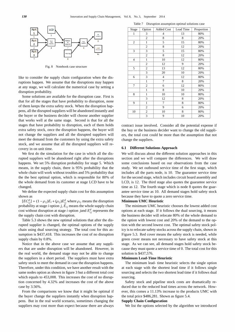
We will discuss about the different solution approaches in thissection and we will compare the differences. We will drawsome conclusions based on our observations from the casestudy. We set outbound service time of the first stage, whichincludes all the parts node, is 10. The guarantee service timefor the second stage, which includes circuit board assembly andLCD, is 12. The third stage also quotes the guarantee servicetime as 12. The fourth stage which is node 8 quotes the guar-antee service time as 10. All demand stages hold safety stockbecause they have to quote a zero service time.Minimum UMC Heuristic

The minimum UMC heuristic chooses the lowest added costoptions at each stage. If it follows the dual sourcing, it meansthe business decider will relocate 80% of the whole demand tothe option with lowest cost and 20% of the demand to the op-tion with the second lowest cost. The optimal safety stock pol-icy is to relocate safety stocks across the supply chain, shown inFigure 5.3. Red cover means the safety stock is needed, whilegreen cover means not necessary to have safety stock at thisstage. As we can see, all demand stages hold safety stock be-cause they must quote a service time of 0. The total cost for thissolution is $437,576.Minimum Lead-Time Heuristic

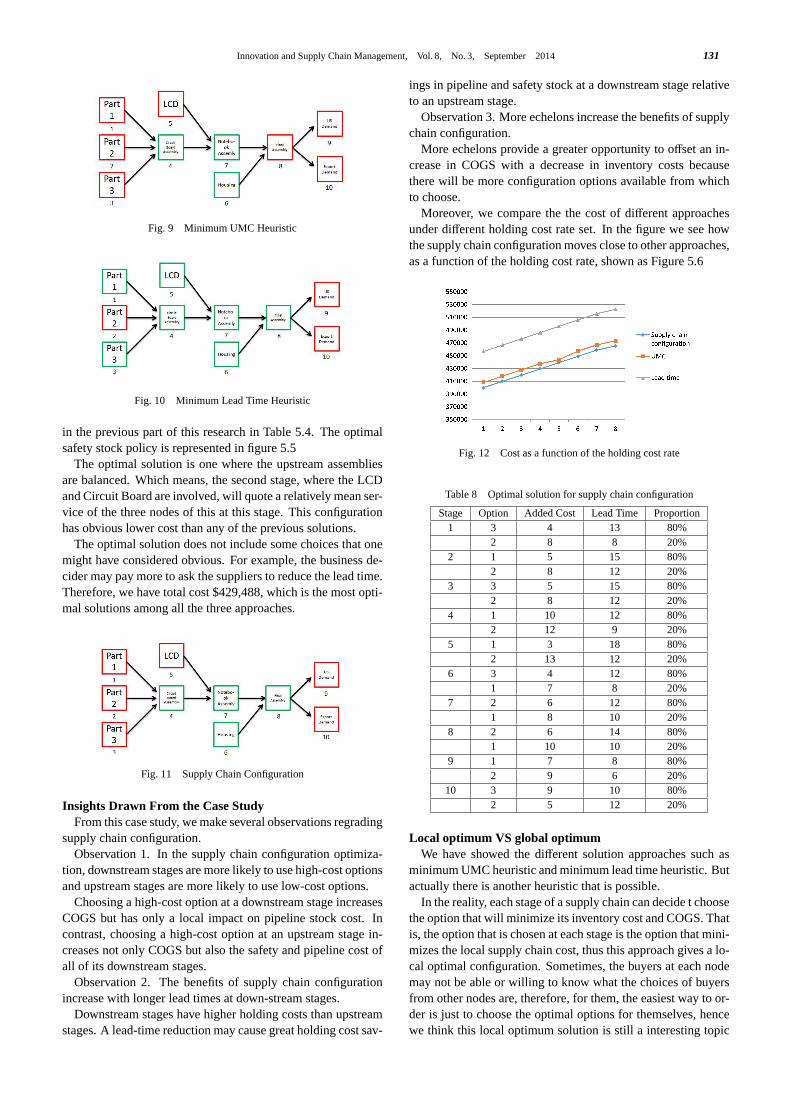
The minimum lead- time heuristic selects the single optionat each stage with the shortest lead time if it follows singlesourcing and selects the two shortest lead time if it follows dualsourcing.

Safety stock and pipeline stock costs are dramatically re-duced due to the reduced lead times across the network. How-ever, this comes a 11.13% increase to the products UMC withthe total price $486,281. Shown as figure 5.4.Supply Chain Configuration

We list the options selected by the algorithm we introduced


Fig. 9 Minimum UMC Heuristic

Fig. 10 Minimum Lead Time Heuristic

in the previous part of this research in Table 5.4. The optimalsafety stock policy is represented in figure 5.5

The optimal solution is one where the upstream assembliesare balanced. Which means, the second stage, where the LCDand Circuit Board are involved, will quote a relatively mean ser-vice of the three nodes of this at this stage. This configurationhas obvious lower cost than any of the previous solutions.

The optimal solution does not include some choices that onemight have considered obvious. For example, the business de-cider may pay more to ask the suppliers to reduce the lead time.Therefore, we have total cost $429,488, which is the most opti-mal solutions among all the three approaches.

Fig. 11 Supply Chain Configuration

Insights Drawn From the Case StudyFrom this case study, we make several observations regrading

supply chain configuration.Observation 1. In the supply chain configuration optimiza-

tion, downstream stages are more likely to use high-cost optionsand upstream stages are more likely to use low-cost options.

Choosing a high-cost option at a downstream stage increasesCOGS but has only a local impact on pipeline stock cost. Incontrast, choosing a high-cost option at an upstream stage in-creases not only COGS but also the safety and pipeline cost ofall of its downstream stages.

Observation 2. The benefits of supply chain configurationincrease with longer lead times at down-stream stages.

Downstream stages have higher holding costs than upstreamstages. A lead-time reduction may cause great holding cost sav-

ings in pipeline and safety stock at a downstream stage relativeto an upstream stage.

Observation 3. More echelons increase the benefits of supplychain configuration.

More echelons provide a greater opportunity to offset an in-crease in COGS with a decrease in inventory costs becausethere will be more configuration options available from whichto choose.

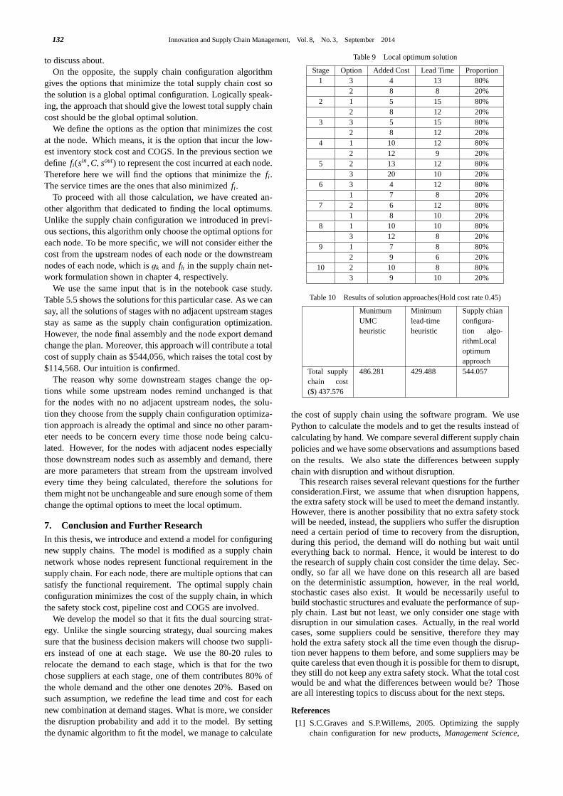
Moreover, we compare the the cost of different approachesunder different holding cost rate set. In the figure we see howthe supply chain configuration moves close to other approaches,as a function of the holding cost rate, shown as Figure 5.6

Fig. 12 Cost as a function of the holding cost rate

Table 8 Optimal solution for supply chain configuration


2 8 8 20%2 1 5 15 80%

2 8 12 20%3 3 5 15 80%

2 8 12 20%4 1 10 12 80%

2 12 9 20%5 1 3 18 80%

2 13 12 20%6 3 4 12 80%

1 7 8 20%7 2 6 12 80%

1 8 10 20%8 2 6 14 80%

1 10 10 20%9 1 7 8 80%

2 9 6 20%10 3 9 10 80%

2 5 12 20%

Local optimum VS global optimumWe have showed the different solution approaches such as

minimum UMC heuristic and minimum lead time heuristic. Butactually there is another heuristic that is possible.

In the reality, each stage of a supply chain can decide t choosethe option that will minimize its inventory cost and COGS. Thatis, the option that is chosen at each stage is the option that mini-mizes the local supply chain cost, thus this approach gives a lo-cal optimal configuration. Sometimes, the buyers at each nodemay not be able or willing to know what the choices of buyersfrom other nodes are, therefore, for them, the easiest way to or-der is just to choose the optimal options for themselves, hencewe think this local optimum solution is still a interesting topic


to discuss about.On the opposite, the supply chain configuration algorithm

gives the options that minimize the total supply chain cost sothe solution is a global optimal configuration. Logically speak-ing, the approach that should give the lowest total supply chaincost should be the global optimal solution.

We define the options as the option that minimizes the costat the node. Which means, it is the option that incur the low-est inventory stock cost and COGS. In the previous section wedefine fi(sin,C, sout) to represent the cost incurred at each node.Therefore here we will find the options that minimize thefi .The service times are the ones that also minimizedfi .

To proceed with all those calculation, we have created an-other algorithm that dedicated to finding the local optimums.Unlike the supply chain configuration we introduced in previ-ous sections, this algorithm only choose the optimal options foreach node. To be more specific, we will not consider either thecost from the upstream nodes of each node or the downstreamnodes of each node, which isgk and fh in the supply chain net-work formulation shown in chapter 4, respectively.

We use the same input that is in the notebook case study.Table 5.5 shows the solutions for this particular case. As we cansay, all the solutions of stages with no adjacent upstream stagesstay as same as the supply chain configuration optimization.However, the node final assembly and the node export demandchange the plan. Moreover, this approach will contribute a totalcost of supply chain as $544,056, which raises the total cost by$114,568. Our intuition is confirmed.

The reason why some downstream stages change the op-tions while some upstream nodes remind unchanged is thatfor the nodes with no no adjacent upstream nodes, the solu-tion they choose from the supply chain configuration optimiza-tion approach is already the optimal and since no other param-eter needs to be concern every time those node being calcu-lated. However, for the nodes with adjacent nodes especiallythose downstream nodes such as assembly and demand, thereare more parameters that stream from the upstream involvedevery time they being calculated, therefore the solutions forthem might not be unchangeable and sure enough some of themchange the optimal options to meet the local optimum.

7. Conclusion and Further ResearchIn this thesis, we introduce and extend a model for configuringnew supply chains. The model is modified as a supply chainnetwork whose nodes represent functional requirement in thesupply chain. For each node, there are multiple options that cansatisfy the functional requirement. The optimal supply chainconfiguration minimizes the cost of the supply chain, in whichthe safety stock cost, pipeline cost and COGS are involved.

We develop the model so that it fits the dual sourcing strat-egy. Unlike the single sourcing strategy, dual sourcing makessure that the business decision makers will choose two suppli-ers instead of one at each stage. We use the 80-20 rules torelocate the demand to each stage, which is that for the twochose suppliers at each stage, one of them contributes 80% ofthe whole demand and the other one denotes 20%. Based onsuch assumption, we redefine the lead time and cost for eachnew combination at demand stages. What is more, we considerthe disruption probability and add it to the model. By settingthe dynamic algorithm to fit the model, we manage to calculate

Table 9 Local optimum solution


2 8 8 20%2 1 5 15 80%

2 8 12 20%3 3 5 15 80%

2 8 12 20%4 1 10 12 80%

2 12 9 20%5 2 13 12 80%

3 20 10 20%6 3 4 12 80%

1 7 8 20%7 2 6 12 80%

1 8 10 20%8 1 10 10 80%

3 12 8 20%9 1 7 8 80%

2 9 6 20%10 2 10 8 80%

3 9 10 20%

Table 10 Results of solution approaches(Hold cost rate 0.45)

MunimumUMCheuristic

Minimumlead-timeheuristic

Supply chianconfigura-tion algo-rithmLocaloptimumapproach

Total supplychain cost($) 437.576

486.281 429.488 544.057

the cost of supply chain using the software program. We usePython to calculate the models and to get the results instead ofcalculating by hand. We compare several different supply chainpolicies and we have some observations and assumptions basedon the results. We also state the differences between supplychain with disruption and without disruption.

This research raises several relevant questions for the furtherconsideration.First, we assume that when disruption happens,the extra safety stock will be used to meet the demand instantly.However, there is another possibility that no extra safety stockwill be needed, instead, the suppliers who suffer the disruptionneed a certain period of time to recovery from the disruption,during this period, the demand will do nothing but wait untileverything back to normal. Hence, it would be interest to dothe research of supply chain cost consider the time delay. Sec-ondly, so far all we have done on this research all are basedon the deterministic assumption, however, in the real world,stochastic cases also exist. It would be necessarily useful tobuild stochastic structures and evaluate the performance of sup-ply chain. Last but not least, we only consider one stage withdisruption in our simulation cases. Actually, in the real worldcases, some suppliers could be sensitive, therefore they mayhold the extra safety stock all the time even though the disrup-tion never happens to them before, and some suppliers may bequite careless that even though it is possible for them to disrupt,they still do not keep any extra safety stock. What the total costwould be and what the differences between would be? Thoseare all interesting topics to discuss about for the next steps.

References

[1] S.C.Graves and S.P.Willems, 2005. Optimizing the supplychain configuration for new products,Management Science,


51(8), 1165-1180.[2] S.C.Graves and S.P.Willems, 2000. Optimizing strategic safety

stock placement in supply chains,Manufacturing and ServiceOperations Management, 2(1), 68-83.

[3] F.S.Hillier and G.J.Lieberman, 2005. Introduction to opera-tions research, eighth edition, McGraw-Hill.

[4] Junlin Chen, Han Zhao and Xiaobo Zhao, 2012. How probabil-ity weighting affects inventory management with supply dis-ruptions,Proceedings of International MultiConference of En-gineers and Computer Scientists 2012, March, 14-16.

[5] Fred Janssen and Ton de Kok, 1996. A two-supplier inventorymodel, Department of Technology Management, EindhovenUniversity of Technology.

[6] Stefan Minner, 1997. Dynamic programming algorithm formulti-stage safety stock optimization,OR Spektrum 1997, 19,261-271.

[7] Humair and Willems, 2006. Optimizing strategic safety stockplacement in supply chains with clusters of commonal-ity,Operations Research, 54(4), 725-742.

[8] Inderfurth,K, 1993. Valuation of leadtime reduction in multi-stage production systems. G. Fandel, T. Gulledge, A. Jones,eds.,Operation Research in Production Planning and Inven-tory Control, Springer, Berlin, Germany, 413-427.

[9] Ettl, M., G. E. Feigin, G. Y. Lin, D. D. Yao, 2000. A supplynetwork model with base-stock control and service require-ments,Operation Research, 48(2), 216-232.

[10] Geoffrion, A. M.,R. F. Powers, 1995. Twenty years of strategicdistribution system design: an evolutionary perspective,Inter-faces, 25(5), 105-127.

[11] Herbert Scarf, 1959. The optimality of (S,s) policies in thedynamic inventory problem,Technical Report No.11, AppliedMathematics and Statistics Laboratory, Stanford University,Stanford California.

Ruiqing X IA

received Bachelor degree on Software Engineering inNorthwest University in Xi’an, China, and received Mas-ter degree from Keio University. During bachelor study,he specialized in software techniques, coding and projectmanagement. He became master course student since2012, financially supported by scholarship provided byJASSO and Donghua Educational & Cultural Exchange

Foundation of Japan. During the master study, he focused on supply chainmanagement, attended and presented research achievement in Japan Indus-try Management Association annual conference, and presented extendedresearch in ICAOR 2014 entitled“Optimizing Supply Chain Configura-tion with Supply Disruptions. Now he is working at Apple Inc. as anoperations specialist.

Tang LIU

is now PhD candidate in Keio University, Departmentof Administration Engineering, Tokyo, Japan. He re-ceived Master degree from Kobe University, Japan, in2013. His research interests include supply chain riskmanagement under disruption event and supply chain re-silience.

Hiroaki M ATSUKAWA

is a professor at Keio University. He received hisPhD degrees from Tokyo Institute of Technology, Tokyo,Japan, in 1992. Main research interests include produc-tion & inventory control and supply chain management(SCM). Continuous effort is dedicated to clarify prin-ciples of management on those research topics such asscheduling, manufacturing strategy, project management

and other topics related to production and logistics. Quantitative methodswere frequently applied for solving management problems. Recent inter-ests include supply chain risk management under disruptive event, and en-ergy supply control applying supply chain optimization approaches.

Documents

Optimizing Supply Chain Conﬁguration Considering Supply