OPTIMIZING TECHNOLOGY TO REDUCE MERCURY AND ACID GAS EMISSIONS

OPTIMIZING TECHNOLOGY TO REDUCE MERCURY AND ACID GAS EMISSIONS

FROM ELECTRIC POWER PLANTS

Semi-Annual Report February 1, 2004 to July 31, 2004

Principal Authors Jeffrey C. Quick David E. Tabet Sharon Wakefield Roger L. Bon Published August 2004 Prepared for The United States Department of Energy Contract No. DE-FG26-03NT41901 Contract Officer Sara M. Pletcher National Energy Technology Laboratory Morgantown, West Virgina Prepared by The Utah Geological Survey 1594 West North Temple, Suite 3110 Salt Lake City, Utah 84114-6100 (801) 537-3300

DISCLAIMER This report was prepared as an account of work sponsored by an agency of the United States Government. Neither the United States Government nor any agency thereof, nor any of their employees, makes any warranty, express or implied, or assumes any legal liability or responsibility for the accuracy, completeness, or usefulness of any information, apparatus, product, or process disclosed, or represents that its use would not infringe privately owned rights. Reference herein to any specific commercial product, process, or service by trade name, trademark, manufacturer, or otherwise does not necessarily constitute or imply its endorsement, recommendation, or favoring by the United States Government or any agency thereof. The views and opinions of authors expressed herein do not necessarily state or reflect those of the United States Government or any agency thereof. Although this product represents the work of professional scientists, the Utah Department of Natural Resources, Utah Geological Survey, makes no warranty, expressed or implied, regarding its suitability for a particular use. The Utah Department of Natural Resources, Utah Geological Survey, shall not be liable under any circumstances for any direct, indirect, special, incidental, or consequential damages with respect to claims by users of this product.

i

ABSTRACT

County-average hydrogen values are calculated for the part 2, 1999 Information

Collection Request (ICR) coal-quality data, published by the U.S. Environmental Protection

Agency. These data are used together with estimated, county-average moisture values to

calculate average net heating values for coal produced in U.S. counties. Finally, 10 draft maps of

the contiguous U.S. showing the potential uncontrolled sulfur, chlorine and mercury emissions of

coal by U.S. county-of-origin, as well as expected mercury emissions calculated for existing

emission control technologies, are presented and discussed.

TABLE OF CONTENTS

INTRODUCTION .......................................................................................................................... 1

Background................................................................................................................................. 1 Recent Developments ................................................................................................................. 2 Scope of This Report .................................................................................................................. 3

EXECUTIVE SUMMARY ............................................................................................................ 4

EXPERIMENTAL.......................................................................................................................... 6

Calculation of the Net Heating Value (Task 4) ......................................................................... 7 Predicting ICR Coal Hydrogen Values................................................................................... 7 Verification of Equations to Predict Coal Hydrogen............................................................ 13 Verification of Calculated ICR Net Heating Values............................................................. 15

Parameters for Mapping and Draft Maps (Tasks 5 and 6)........................................................ 17 RESULTS AND DISCUSSION................................................................................................... 29

Evaluation of Coal Assay Data ............................................................................................. 29 Evaluation of Technology-Specific Hg Emissions ............................................................... 39

CONCLUSIONS........................................................................................................................... 41

REFERENCES ............................................................................................................................. 42

ii

FIGURES

Figure 1. Schedule of project tasks .................................................................................................4

Figure 2. Emissions expressed on an output basis are best estimated if the fuel emission factor is

expressed on a net energy basis ......................................................................................6

Figure 3. Variation of coal hydrogen with coal rank ......................................................................9

Figure 4. COALQUAL moisture values are lower than moisture values for other data sets .......10

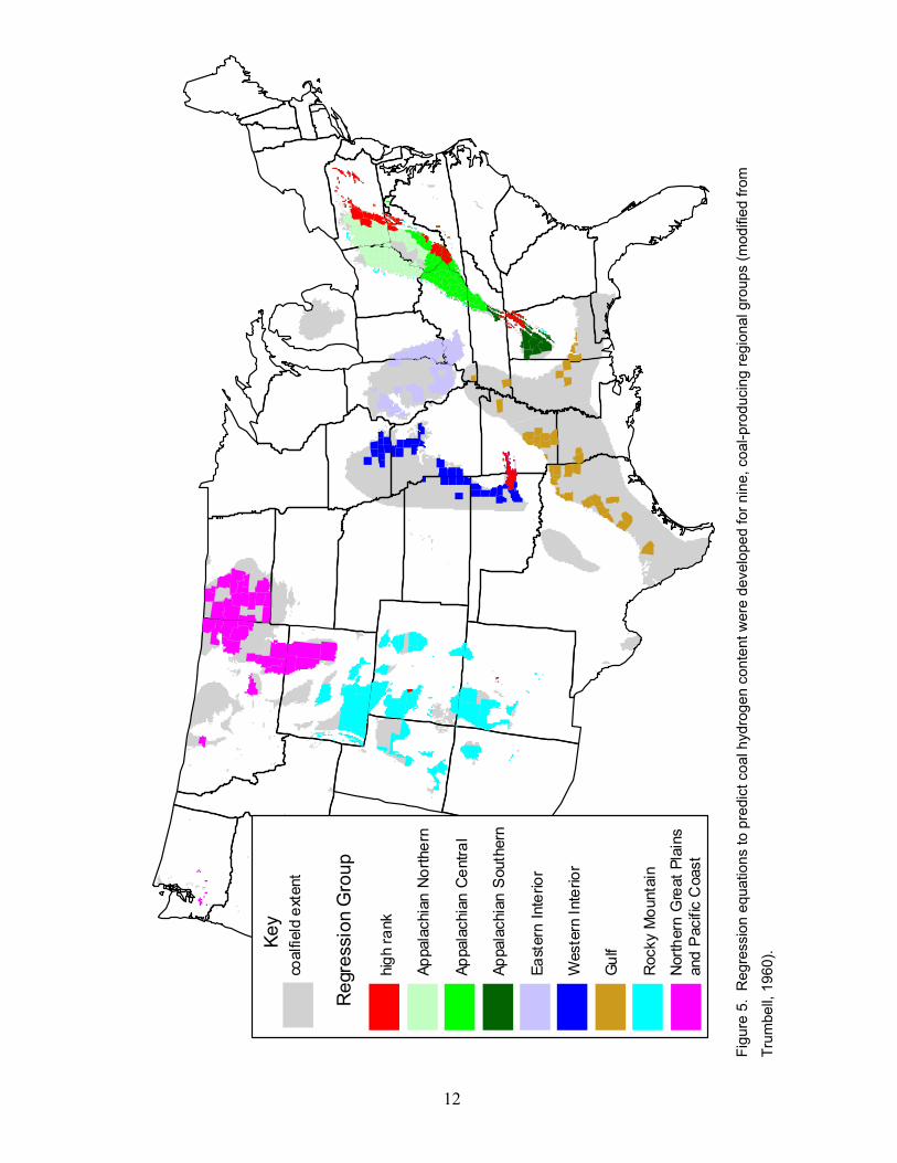
Figure 5. Regression equations to predict coal hydrogen content were developed for nine, coal-

producing regional groups.............................................................................................12

Figure 6. A near 1:1 relationship is observed between the measured PSU-DOE hydrogen values

and predicted PSU-DOE hydrogen values....................................................................15

Figure 7. The difference between the net and gross heating value of U.S. coal from two data sets

systematically varies with ASTM (1990) coal rank......................................................16

Figure 8. Potential uncontrolled sulfur emissions.........................................................................19

Figure 9. Potential uncontrolled mercury emissions.....................................................................20

Figure 10. Potential uncontrolled chlorine emissions by...............................................................21

Figure 11. Predicted mercury emissions for coal burned in electric utilities with Cold-Side,

Electrostatic Precipitators..............................................................................................22

Figure 12. Predicted mercury emissions for coal burned in electric utilities with Cold-Side,

Electrostatic Precipitators and Flue Gas Desulfurization controls................................23

Figure 13. Predicted mercury emissions for coal burned in electric utilities with Hot-Side,

Electrostatic Precipitators..............................................................................................24

Figure 14. Predicted mercury emissions for coal burned in electric utilities with Hot-Side,

Electrostatic Precipitators and Flue Gas Desulfurization..............................................25

Figure 15. Predicted mercury emissions for coal burned in electric utilities with Spray-Dry

Adsorption and fabric filters .........................................................................................26

iii

Figure 16. Predicted mercury emission rate (lbs Hg/terawatt-hour) for coal burned in electric

utilities with Cold-Side, Electrostatic Precipitators and wet Flue Gas Desulfurization

controls..........................................................................................................................27

Figure 17. Predicted mercury emission rate (lbs Hg/terawatt-hour) for coal burned in electric

utilities with Spray-Dry Adsorption and Fabric Filter controls ....................................28

Figure 18. Histograms showing the distribution of county-average coal quality values for the

COALQUAL, FERC 423, ICR, and CTRDB data sets ................................................30

Figure 19. Cross-plots comparing the county-average moisture, ash, sulfur, and Btu values from

the ICR data set with those from the CTRDB, COALQUAL, and FERC 423

data sets .........................................................................................................................31

Figure 20. Distribution of county-average, mercury, chlorine and sulfur values on an energy

basis for the in-ground coal resource and commercial coal shipments.........................34

Figure 21. Comparison of mercury, chlorine, and sulfur values in the ICR and COALQUAL data

sets.................................................................................................................................34

Figure 22. The difference between the mercury content of in-ground coal and the mercury

content of mined coal varies geographically.................................................................37

Figure 23. Average chlorine content of coal delivered to U.S. power plants during 1999, by

county-of-origin ............................................................................................................38

Figure 24. Five model equations predict increasing mercury capture by fabric filter emission

controls with increasing coal chlorine concentration....................................................41

TABLES Table 1. Proposed MACT mercury emission limits .......................................................................2

Table 2. List of variables, coefficients, and statistics for regression equations used to predict coal

hydrogen content .............................................................................................................14

Table 3. Selected parameters for mapping....................................................................................18

1

INTRODUCTION

Background

Switching to low-mercury-emission coal may be an effective strategy to comply with

impending regulations that are intended to reduce mercury emissions from electric utilities. For

example, despite proven emission control technology, burning low-sulfur coal is the most

popular method to reduce sulfur emissions. Because technology to reduce mercury emissions is

considerably less certain, burning low-mercury coal is a likely method to reduce mercury

emissions. Like sulfur, the amount of mercury in U.S. coal shows substantial geographic

variation. Furthermore, mercury emissions from similar types of power plants are largely

correlated with the amount of mercury in the coal. However, unlike sulfur, mercury emissions

also vary with the abundance of other elements in the coal such as chlorine and sulfur, which

influence mercury capture by emission control technologies. Consequently, mercury emission

factors vary according to the relative abundance of several elements in the coal, and are specific

to different emission control technologies.

This project is using Geographic Information System technology (ArcView GIS) to

create detailed maps to show where U.S. coal with low mercury and acid-gas emissions might be

found. The map series will show geographic variation of mercury, chlorine, and sulfur in coal,

as well as the mercury emission penalty calculated for data aggregated by U.S. county-of-origin

using equations specific to power plants classified by boiler type and flue gas emission controls.

Removing mercury from flue gas is a technically complex task – different technologies will be

required for different coals. Maps showing the geographic variation of mercury and acid gas

emission factors for U.S. coal will help locate the best coal for each technology and identify the

best technology for each coal.

2

Coal quality data used in this study were described in a previous report (Quick and

others, 2004). Briefly, these data were selected from five data sets and include: 19,507 FERC

423 data records (USEIA, 2003a), 25,818 ICR data records (USEPA, 2003), 5,602 CTRDB data

records (USEIA, 2003b), 5,045 COALQUAL data records (Bragg and others, 1997), and 73

PSU-DOE data records (Anonymous, 1990; Davis and Glick, 1993; Scaroni and others, 1999).

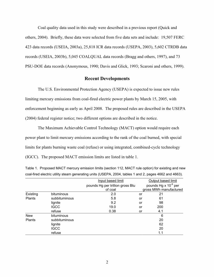
Recent Developments

The U.S. Environmental Protection Agency (USEPA) is expected to issue new rules

limiting mercury emissions from coal-fired electric power plants by March 15, 2005, with

enforcement beginning as early as April 2008. The proposed rules are described in the USEPA

(2004) federal register notice; two different options are described in the notice.

The Maximum Achievable Control Technology (MACT) option would require each

power plant to limit mercury emissions according to the rank of the coal burned, with special

limits for plants burning waste coal (refuse) or using integrated, combined-cycle technology

(IGCC). The proposed MACT emission limits are listed in table 1.

Table 1. Proposed MACT mercury emission limits (section 112, MACT rule option) for existing and new

coal-fired electric utility steam generating units (USEPA, 2004, tables 1 and 2, pages 4662 and 4663).

Input based limit Output based limit

pounds Hg per trillion gross Btu

of coal pounds Hg x 10-6 per

gross MWh manufacturedExisting bituminous 2.0 or 21 Plants subbituminous 5.8 or 61 lignite 9.2 or 98 IGCC 19.0 or 200 refuse 0.38 or 4.1 New bituminous 6 Plants subbituminous 20 lignite 62 IGCC 20 refuse 1.1

3

The cap-and-trade option would limit total mercury emissions from all power plants to a

maximum 15 tons per year by 2018. Each power plant would be required to have mercury

emission allowances sufficient to equal its annual mercury emissions. The allowances would be

distributed by state or federal administrators, and could be used, saved, purchased, or sold. The

USEPA (2004) cap-and-trade proposal allocates allowances to U.S. States according to their

proportional share of coal energy consumption, modified by the rank of the coal consumed. A

state’s fractional share of the proposed 15-ton cap would be calculated as its average coal energy

consumption (highest annual average for 3 of 4 years between 1998 and 2002, of the summed

energy content of coal burned in electric utilities), multiplied by a factor of 1 for bituminous,

1.25 for subbituminous, and 3 for lignite rank coal, and finally divided by the sum of the results

calculated for all 50 states. Additionally, under the cap-and-trade rule, newly constructed power

plants would need to meet the same standards as those listed in table 1 for new plants under the

proposed MACT rule. Although the form of the final rule remains uncertain, the proposed

emission limits shown in table 1 are useful benchmarks to evaluate the geographic variation of

potential mercury emissions.

Scope of This Report

This report describes the progress made during the second six months of this 24-month

project. Results of tasks 4, 5, and 6 (figure 1) are described and discussed.

4

8 9 10 11 12 1 2 3 4 5 6 7 8 9 10 11 12 1 2 3 4 5 6 7

(8) Technical transfer

(7) Create final maps

(6) Create draft maps

(5) Select parameters for mapping

(4) Calculate net heating value

(3) Estimate moisture

(2) Select data

(1) Assemble data

2003 2004 2005

C

W WW W

Advisory board meetingC

W Update project website

THIS REPORT

Figure 1. Schedule of project tasks.

EXECUTIVE SUMMARY

Draft maps showing the geographic variation of mercury and acid gas emission factors

for U.S. coals were constructed using coal assay data aggregated by U.S. county-of-origin.

Specific tasks accomplished during the second six months of this two-year project include:

• Coal hydrogen values were estimated for the ICR data using equations based on selected

COALQUAL data records.

• Net coal heating values were calculated for the ICR data by U.S. county-of-origin.

• Published emission factors that predict mercury capture for power plants classified by air

pollution controls were selected and applied to the ICR data.

• Draft maps were made using ICR data aggregated by county-of-origin. The maps show

potential uncontrolled mercury, sulfur, and chlorine emissions, as well as predicted

mercury emissions from coal burned in power plants classified by air pollution controls.

5

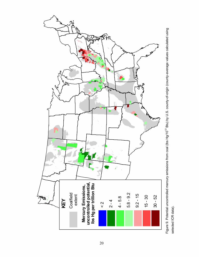
• High-mercury coal is produced in parts of Oklahoma, Texas, Ohio, Pennsylvania,

Kentucky, Alabama, and Tennessee, whereas low-mercury coal is common in the western

U.S., Eastern Interior Province, and the Central Appalachian Region.

• Coal from the Northern Appalachian Region (Ohio and parts of Pennsylvania) has notably

high mercury concentrations compared to U.S. coal produced elsewhere.

• Much subbituminous and some lignite coal should comply with the proposed MACT rule

using existing technology. Bituminous compliance coal for power plants with Electrostatic

Precipitator (ESP) controls is rare. Plants equipped with Flue Gas Desulfurization (FGD)

controls may find bituminous compliance coal in some western U.S. counties, the Eastern

Interior Province, and the Central Appalachian Region. With notable exceptions (for

example, numerous counties in Ohio and the western U.S.), fabric filters may be an

effective technology for bituminous coal.

6

EXPERIMENTAL

The proposed MACT rule includes both input-based (pounds Hg per trillion Btu) and

output-based (pounds Hg x 10-6 per megawatt-hour electricity manufactured) emission limits

(table 1). The output-based limits assume 32 percent efficiency (10,667 gross Btu/kilowatt-hour)

for existing power plants and 35 percent efficiency (9,833 gross Btu/kilowatt-hour) for new

power plants (USEPA, 2004). Although the USEPA used the gross heating value of coal1 to

calculate the output-based emission limits (Cole, 2003), figure 2 shows that output-based

emissions are better calculated from fuel emission factors expressed on a net energy basis.

Accordingly, we use emission factors expressed on a net energy basis to calculate output-based

emissions. This required that we calculate county-average, ICR net heating values.

Figure 2. Emissions expressed on an output basis (vertical axes) are better estimated if the fuel emission

factor is expressed on a net energy basis (right plot) rather than on a gross energy basis (left plot). Data

show output-based carbon emissions calculated by Juniper (1998) for commercial coals in a model 500

MW plant equipped with ESP and FGD emissions controls.

1 The gross coal heating value, (also called the higher heating value) is the familiar Btu/lb (or MJ/kg) value reported from the laboratory. The gross heating value is measured by using a high-pressure, constant-volume combustion bomb. Because water vapor from combustion condenses inside the combustion bomb the gross heating value includes the latent heat of water vapor. Unlike the laboratory combustion bomb, combustion in a coal-fired boiler occurs at constant pressure and moisture from combustion exits the boiler with the flue gas. Consequently, the net heating value (also called the lower heating value) does not include the latent heat of water vapor and is a better measure of the energy available to the boiler than the gross heating value.

7

Calculation of the Net Heating Value (Task 4)

The net heating value is calculated as:

( )HMBtuBtu grossnet +−= 1119.07.92 (1)

where: Btu gross is the familiar Btu per pound value reported from the laboratory and expressed on

a moist, whole-coal basis,

M is the weight percent moisture content of the coal,

H is the weight percent hydrogen of the coal (not including hydrogen in coal moisture)

expressed on a moist, whole-coal basis,

0.1119 is the gravimetric factor applied to the moisture value (M) to obtain the weight

percent hydrogen in coal moisture and,

92.7 is the Btu penalty, which is largely due to the latent heat of water vapor, which is

lost from the boiler with the combustion flue gas.

Note that the ICR data do not include moisture or hydrogen values, which are required for

equation 1. County-average, ICR moisture values were estimated in an earlier report (Quick and

others, 2004). County-average ICR hydrogen values were calculated using predictive equations

obtained by regression analysis, which is described below.

Predicting ICR Coal Hydrogen Values

A multivariate regression method was applied to selected COALQUAL data (Mott-

Spooner values within ±250 Btu) to develop a set of geographically specific equations to predict

coal hydrogen content using dry-basis Btu/lb, ash, and sulfur values. The equations were

validated using the PSU-DOE data, and used to estimate ICR coal hydrogen values.

The dependent COALQUAL variable was dry-basis hydrogen. Note that moist-basis

hydrogen values, which include hydrogen in coal moisture, are listed in the COALQUAL data

8

set. Consequently, the COALQUAL hydrogen values were adjusted to a dry basis by subtracting

the stochiometric contribution of water to hydrogen (0.1119 x moisture), and multiplying the

result by moisture−100100 (ASTM, 2000a).

The four independent variables used in the regression analysis (Btudmmf, Btudmmf2, MMParr, dry,

and lbs S/million Btu) were calculated for the selected COALQUAL data records using the

equations:

( ))55.008.1(100

50100

drydry

drydrydmmf

SAsh

SBtuBtu

+−

−×= (2)

dmmfdmmfdmmf BtuBtuBtu ×=2 (3)

drydrydryParr SAshMM 55.008.1, += (4)

100106

dry

dry

SBtu

BtumillionSlbs ×= (5)

where, Btudry is the dry-basis Btu per pound value,

Sdry is the dry-basis weight percent sulfur, and

Ashdry is the dry-basis weight percent ash.

Although the regression equations were obtained using relationships observed in the

COALQUAL data, they were used to predict ICR coal hydrogen values. Consequently, the

selection of the independent variables was necessarily constrained by the available ICR assay

data (Btu/lb, ash, S, Cl, Hg, and estimated moisture). Considering this constraint, the

independent variables were selected to indicate coal rank, (Btudmmf and Btudmmf2), coal grade

(MMParr,dry), and coal type (lbs S/million Btu), all of which may influence the hydrogen content of

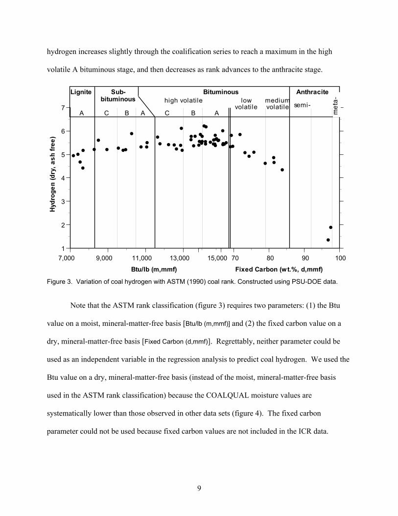
coal. For example, the influence of coal rank is illustrated in figure 3, which shows that coal

9

hydrogen increases slightly through the coalification series to reach a maximum in the high

volatile A bituminous stage, and then decreases as rank advances to the anthracite stage.

Btu/lb (m,mmf) Fixed Carbon (wt.%, d,mmf)

••

••••

•••

•••••

70 80 90 100

•

••

••••••

••

• ••

• ••

•• ••

••• ••

•

•• ••

• • •••••••

•• ••• ••••••

•

1

2

3

4

5

6

7

7,000 9,000 11,000 13,000 15,000

Lignite Sub-bituminous

Bituminous Anthracite

A AAB BC C

high volati le lowvolatile

mediumvolatile semi-

Figure 3. Variation of coal hydrogen with ASTM (1990) coal rank. Constructed using PSU-DOE data.

Note that the ASTM rank classification (figure 3) requires two parameters: (1) the Btu

value on a moist, mineral-matter-free basis [Btu/lb (m,mmf)] and (2) the fixed carbon value on a

dry, mineral-matter-free basis [Fixed Carbon (d,mmf)]. Regrettably, neither parameter could be

used as an independent variable in the regression analysis to predict coal hydrogen. We used the

Btu value on a dry, mineral-matter-free basis (instead of the moist, mineral-matter-free basis

used in the ASTM rank classification) because the COALQUAL moisture values are

systematically lower than those observed in other data sets (figure 4). The fixed carbon

parameter could not be used because fixed carbon values are not included in the ICR data.

10

•

•

••••

•

• ••

•••

•• •

•

•••••

•

•

•

•

• •••

•

•

•

••

•

•

•

••

•

•

•

•

•

•

•

•

•

••

••••• •

••••••

••••• •••

•••• ••

•• •• ••• •• ••••

•

•

•

•

••

•••

•

•••••••••

••••

•••••••

•

••

••

•••

••••

•••

•

•

••

••

•

•

•

•

••

•••

•

+++

++++ +

+++ +++ +

++

++++

+

++

+

++

+

+

+

+

+ ++++

+

+

+

++

+

+

+

+

++

+

+

+

+

+

+

+

+

+

+

++

+

+

+++++++++++++

++++++++++++++++++

++++++++++++++

♦

♦♦

♦♦♦♦♦♦

♦♦♦♦

♦♦

♦

♦♦

♦♦

♦♦♦♦

♦♦

♦

♦♦

♦

♦

♦

♦

♦

♦

♦

♦♦

♦

♦♦

♦♦

♦

♦

♦♦

♦♦

♦

♦

♦

♦

♦

♦

♦

♦♦

♦

♦

∆∆∆∆∆∆∆∆∆∆

∆∆∆∆∆∆∆∆∆∆∆∆∆∆∆∆∆∆∆∆∆∆∆∆∆∆∆∆∆∆

∆

∆∆∆∆∆∆

∆∆∆∆∆∆∆∆∆∆∆

∆

∆∆∆

∆

∆∆∆∆∆∆

∆

∆∆∆∆∆∆∆∆∆∆∆∆∆∆∆∆∆∆∆

∆

∆∆∆

∆

∆∆

∆

∆∆

∆

∆∆

∆

∆∆∆∆∆∆∆

∆∆

∆∆

∆

∆

∆

∆

∆∆∆

∆

∆

∆

∆∆∆

∆

∆

∆∆

∆

∆

∆

∆

∆∆

∆

∆∆

∆

∆∆

∆

∆

∆∆

∆

∆

∆∆∆∆∆

∆

∆

∆∆

∆

∆

∆∆∆∆∆∆∆

∆

∆

∆∆

∆

∆

∆

∆

∆

∆

∆∆∆∆

∆

∆

∆

∆

∆

∆

∆

∆∆

∆

∆

∆

∆

∆

∆

∆

∆

∆

∆

∆

∆

∆∆

∆∆

∆

∆

∆

∆

∆∆

∆

∆

∆∆

∆

∆

∆

∆

∆

∆

∆∆

∆

∆

∆

∆

∆∆

∆

∆

∆

∆

∆∆

∆

∆

∆

∆

∆

∆

∆∆

∆

0

10

20

30

40

50

12,000 13,000 14,000 15,000 16,000

• ICR

+ CTRDB

♦ PSU-DOE

∆ COALQUAL

DATA KEY

Btu/lb (dry, mineral-matter-free)

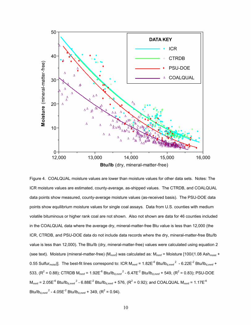
Figure 4. COALQUAL moisture values are lower than moisture values for other data sets. Notes: The

ICR moisture values are estimated, county-average, as-shipped values. The CTRDB, and COALQUAL

data points show measured, county-average moisture values (as-received basis). The PSU-DOE data

points show equilibrium moisture values for single coal assays. Data from U.S. counties with medium

volatile bituminous or higher rank coal are not shown. Also not shown are data for 46 counties included

in the COALQUAL data where the average dry, mineral-matter-free Btu value is less than 12,000 (the

ICR, CTRDB, and PSU-DOE data do not include data records where the dry, mineral-matter-free Btu/lb

value is less than 12,000). The Btu/lb (dry, mineral-matter-free) values were calculated using equation 2

(see text). Moisture (mineral-matter-free) (Mmmf) was calculated as: Mmmf = Moisture [100/(1.08 Ashmoist +

0.55 Sulfurmoist)]. The best-fit lines correspond to: ICR Mmmf = 1.82E-6 Btu/lbd,mmf 2 - 6.22E-2 Btu/lbd,mmf +

533, (R2 = 0.88); CTRDB Mmmf = 1.92E-6 Btu/lbd,mmf 2 - 6.47E-2 Btu/lbd,mmf + 549, (R2 = 0.83); PSU-DOE

Mmmf = 2.05E-6 Btu/lbd,mmf 2 - 6.88E-2 Btu/lbd,mmf + 576, (R2 = 0.92); and COALQUAL Mmmf = 1.17E-6

Btu/lbd,mmf 2 - 4.05E-2 Btu/lbd,mmf + 349, (R2 = 0.94).

11

The relationship between coal rank and coal hydrogen (figure 3) also shows that

hydrogen declines at higher ranks with increasing fixed carbon. The sharp decline of hydrogen

at high rank shown in figure 3 shows that different equations are required for high and low-rank

coals. Accordingly, fixed carbon values listed in the COALQUAL data were used to identify

U.S. counties with high-rank coal. COALQUAL data values from these counties (Btudmmf,

Btudmmf2, MMParr,dry, and lbs S/million Btu values) were used to establish equations to predict the

hydrogen content of high-rank coal, and the equations were applied to the ICR data originating

from the same counties.

Attempts to develop a single equation to predict hydrogen for high volatile A bituminous

(hvAb) and lower rank coals gave unsatisfactory results. The results overestimated coal

hydrogen in some geographic regions and underestimated coal hydrogen in others. For example,

the multiple regression equation based on all the COALQUAL data for hvAb and lower rank

coal, showed average residuals of -0.15% hydrogen for Western Interior coal and +0.23%

hydrogen for Gulf Coast coal. To avoid these systematic errors, equations to predict coal

hydrogen were determined for coal from each of the geographic regions shown in figure 5.

The regression equations used to predict coal hydrogen in this report are described in

table 2. Several results are noteworthy. Excluding high-rank coal, relatively large t-statistic

values, and consistently negative coefficients for the coal grade parameter (MMParr,dry) show the

strong influence of mineral matter content on coal hydrogen; coal hydrogen declines with

increasing mineral content. The general lack of significance (t-statistic <2) for the rank

parameter (Btudmmf) for coal from the Northern Great Plains and the High Rank groups may be

due to small range of variation of the Btu variable in coal from these areas. Although the type

parameter (lbs S/million Btu) is typically the least significant of the independent variables, its

12

Appa

lach

ian

Nor

ther

n

Appa

lach

ian

Cen

tral

Appa

lach

ian

Sou

ther

n

East

ern

Inte

rior

Wes

tern

Inte

rior

Gul

f

Roc

ky M

ount

ain

Nor

ther

n G

reat

Pla

ins

and

Pac

ific

Coa

st

high

rank

Reg

ress

ion

Gro

up

coal

field

ext

ent

Key

Figu

re 5

. R

egre

ssio

n eq

uatio

ns to

pre

dict

coa

l hyd

roge

n co

nten

t wer

e de

velo

ped

for n

ine,

coa

l-pro

duci

ng re

gion

al g

roup

s (m

odifi

ed fr

om

Trum

bell,

196

0).

13

generally positive coefficient is consistent with the geologic enrichment of coal hydrogen due to

the preservation of otherwise labile hydrogen-rich compounds by an early diagenetic natural

vulcanization process where aliphatic compounds are cross-linked by hydrogen sulfide from

sulfate-reducing bacteria (Sinninghe Damste and others, 1989). The inability of the sulfur

variable to predict coal hydrogen for coal from 5 of the 9 groups (t-statistic <2) is also

noteworthy and may have varied origins; possibilities include (1) a late-stage abiogenic sulfide

contribution to Western Interior coal (after diagenetic loss of labile hydrogen), (2) greater initial

hydrogen of geologically younger (western U.S.) peat-forming biomass (more H-rich cellulose;

Robinson, 1990) with early bacterial stripping of hydrogen by methanogenic bacteria, which

thrive in the absence of dissolved sulfate (Belyaev and others, 1980), and (3) catagenetic loss of

hydrogen associated with sulfur in aliphatic structures, as aliphatic sulfur is lost or transformed

into aromatic sulfur at higher ranks (Maes and others, 1997; Gorbaty and Kelemen, 2001).

Verification of Equations to Predict Coal Hydrogen

The geographically specific equations used to predict coal hydrogen are described in

table 2. These equations were applied to the PSU-DOE data to verify their accuracy. Figure 6

shows the near 1:1 correspondence between the measured PSU-DOE hydrogen values and the

predicted PSU-DOE hydrogen values. Error bars on the figure correspond to an assay

reproducibility of 0.3% hydrogen (ASTM, 2000b) and show that most of the scatter can be

attributed to the limited precision of the hydrogen assay. The departure of two, low-hydrogen

coals (anthracite rank) from the forced regression line suggests that the regression model is not

well suited to predict the hydrogen content of anthracite.

14

Table 2. List of variables, coefficients, and statistics for geographically specific regression equations

used to predict the hydrogen content of coal (see equations 2 to 5 in text for variable descriptions).

Data Group variable name coefficient t-statistic equation statistics Intercept -56.22 -14.9 Northern

Appalachian Btudmmf2 -2.82 E-07 -16.4 adjusted R2 = 0.75

Btudmmf 8.35 E-03 16.4 standard error = 0.18 MMParr,dry -5.34 E-02 -49.1 lbs S/million Btu 5.97 E-02 12.0 observations = 1028

Intercept -55.81 -18.1 Central Appalachian Btudmmf

2 -2.76 E-07 -19.5 adjusted R2 = 0.74

Btudmmf 8.22 E-03 19.7 std. error = 0.19 MMParr,dry -5.10 E-02 -39.6 lbs S/million Btu 1.06 E-01 12.7 observations = 756

Intercept -65.88 -13.3 Southern Appalachian Btudmmf

2 -3.19 E-07 -14.3 adjusted R2 = 0.71


Intercept -41.39 -2.8 Eastern Interior Btudmmf

2 -2.11 E-07 -3.0 adjusted R2 = 0.73


Intercept -4.54 -0.6 Western Interior Btudmmf

2 -3.54 E-08 -0.9 adjusted R2 = 0.82


Intercept 20.97 2.5 Gulf Coast Btudmmf

2 1.35 E-07 2.4 adjusted R2 = 0.73

Btudmmf -2.95 E-03 -2.2 std. error = 0.23 MMParr,dry -3.95 E-02 -10.4 lbs S/million Btu -5.27 E-02 -1.9 observations = 66

Intercept -5.87 -5.4 Rocky Mountain Btudmmf

2 -3.39 E-08 -5.7 adjusted R2 = 0.83


Intercept 1.88 0.5 Btudmmf

2 5.98 E-09 0.3 adjusted R2 = 0.72

Btudmmf 1.64 E-04 0.3 std. error = 0.19

Northern Great Plains, Pacific Coast

MMParr,dry -3.88 E-02 -20.4 lbs S/million Btu 3.80 E-03 0.3 observations = 502

Intercept -35.66 5.9 High Rank (mvb to lvb) Btudmmf

2 -1.66 E-07 6.1 adjusted R2 = 0.52

Btudmmf 5.20 E-03 -6.0 std. error = 0.28 MMParr,dry -4.19 E-02 1.4 lbs S/million Btu 3.91 E-02 -1.6 observations = 362

(anthracite) Intercept 209.20 5.9 Btudmmf

2 1.02 E-06 6.1 adjusted R2 = 0.67

Btudmmf -2.92 E-02 -6.0 std. error = 0.38 MMParr,dry 1.74 E-02 1.4 lbs S/million Btu -4.78 E-01 -1.6 observations = 25

15

♦♦

♦♦♦

♦

♦

♦

♦

♦♦

♦♦

♦♦ ♦♦♦♦ ♦♦

♦

♦♦♦ ♦♦♦

♦

♦

♦♦

♦♦♦♦

♦♦♦

♦

♦

♦♦

♦♦

♦♦♦

♦

♦

♦

♦♦♦♦♦♦

♦♦♦♦

♦♦♦

1

2

3

4

5

6

1 2 3 4 5 6

Hpredicted

= 0.99Hmeasured

r2 = 0.88n = 64

std. error = 0.22

Hmeasured (wt.%, dry)

Figure 6. A near 1:1 relationship is observed between the measured PSU-DOE hydrogen values

(Hmeasured) and predicted PSU-DOE hydrogen values (Hpredicted). The predicted hydrogen values were

calculated using equations described in table 2 (in text). The points represent individual PSU-DOE data

records selected to have Mott-Spooner difference values within ±250 Btu. Error bars illustrate an assay

reproducibility of ±0.3% hydrogen (ASTM, 2000b) and show that most of the scatter is explained by the

precision of the hydrogen assay.

Verification of Calculated ICR Net Heating Values

The predicted hydrogen, estimated moisture, and measured Btu values were used with

equation 1 to calculate the average net heating value for 169 counties represented in the ICR data

set. The county-average results show that the net heating value is about 4.5% less than the gross

heating value. This is similar to the 5% difference assumed by the reference method to verify

greenhouse gas emissions for the Kyoto Protocol (Houghton and others, 1997). However, as

shown in figure 7, the difference between the net and gross heating value varies with coal rank.

16

The net heating value of lignite is about 10 percent less than its gross heating value; the

difference smoothly declines through the coalification series to reach a minimum (1 to 2 percent

difference) at the anthracite stage. Figure 7 also shows that the net heating values predicted for

the county-average ICR data mimic those calculated using the (measured) PSU-DOE moisture

and hydrogen values.

70 80 90 100

ο

ο

οο οοοοο ο ο οοοοοο οοο οοοο οο οοοοοο οοοο

οο οοοοο οο οοοο οο οοοοο

ο οο

ο οοοοοοοοοο

οοοοο οο

οοο οοοοοοοο οο οοοο ο

ο ο οοο οο

οοο

ο οοο ο

ο οοο

οο ο

οοοο

οο

οο

οο

οο

ο

οοο

ο

οοοο

ο

ο

οο

οοο ο

ο οο

ο οο

οο

++ +

+

+

++

+++

+

+

+

+

+

++

+

+

+ +

+

+

+++ +++ +

+ + +

+

+

++ + ++ +++ + ++ + ++ ++++

0

2

4

6

8

10

7,000 9,000 11,000 13,000 15,000

ο ICR data

+ PSU-DOE data

Btu/lb (m,mmf) Fixed Carbon (wt.%, d,mmf)

Lignite Sub-bituminous

Bituminous Anthracite

A AAB BC C

high volatile lowvolati le

mediumvolatile semi

-

ICR data from U.S.counties with high rankcoal, where fixedcarbon is theappropriate rankparameter, but was notmeasured for the ICRdata collection effort

Figure 7. The difference between the net and gross heating value of U.S. coal from two data sets

systematically varies with ASTM (1990) coal rank. The percent difference between the gross heating

value of coal (Btugross), and the calculated net heating value (Btunet) corresponds to:

)(100

netgross

gross

BtuBtuBtu

DifferencePercent−

= . The PSU-DOE data points represent single coal assays on an

equilibrium moisture basis. The ICR data points represent county-average values on an estimated, as-

shipped moisture basis.

17

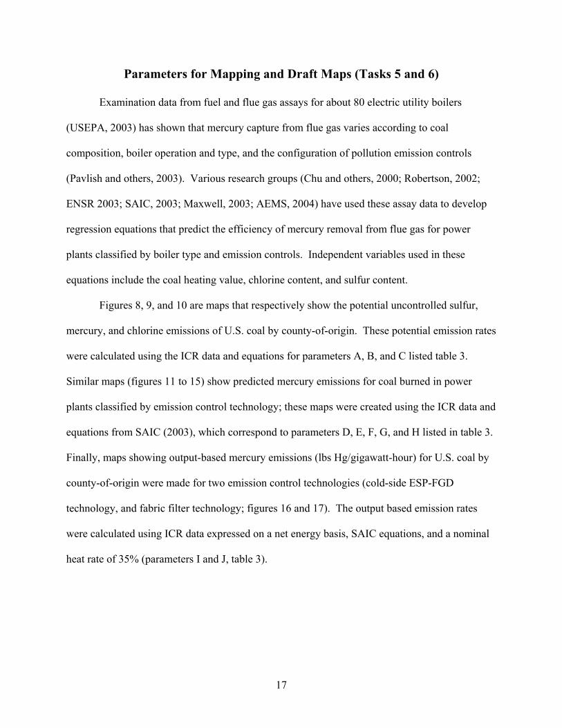
Parameters for Mapping and Draft Maps (Tasks 5 and 6)

Examination data from fuel and flue gas assays for about 80 electric utility boilers

(USEPA, 2003) has shown that mercury capture from flue gas varies according to coal

composition, boiler operation and type, and the configuration of pollution emission controls

(Pavlish and others, 2003). Various research groups (Chu and others, 2000; Robertson, 2002;

ENSR 2003; SAIC, 2003; Maxwell, 2003; AEMS, 2004) have used these assay data to develop

regression equations that predict the efficiency of mercury removal from flue gas for power

plants classified by boiler type and emission controls. Independent variables used in these

equations include the coal heating value, chlorine content, and sulfur content.

Figures 8, 9, and 10 are maps that respectively show the potential uncontrolled sulfur,

mercury, and chlorine emissions of U.S. coal by county-of-origin. These potential emission rates

were calculated using the ICR data and equations for parameters A, B, and C listed table 3.

Similar maps (figures 11 to 15) show predicted mercury emissions for coal burned in power

plants classified by emission control technology; these maps were created using the ICR data and

equations from SAIC (2003), which correspond to parameters D, E, F, G, and H listed in table 3.

Finally, maps showing output-based mercury emissions (lbs Hg/gigawatt-hour) for U.S. coal by

county-of-origin were made for two emission control technologies (cold-side ESP-FGD

technology, and fabric filter technology; figures 16 and 17). The output based emission rates

were calculated using ICR data expressed on a net energy basis, SAIC equations, and a nominal

heat rate of 35% (parameters I and J, table 3).

18

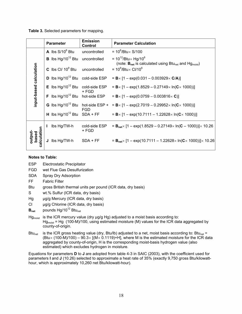
Table 3. Selected parameters for mapping.

Parameter Emission Control Parameter Calculation

A lbs S/106 Btu uncontrolled = 106/Btu× S/100

B lbs Hg/1012 Btu uncontrolled = 1012/Btu× Hg/106 (note: Bnet is calculated using Btunet and Hgmoist)

C lbs Cl/ 109 Btu uncontrolled = 109/Btu× Cl/106

D lbs Hg/1012 Btu cold-side ESP = B× [1 – exp(0.031 – 0.003929× C/A)]

E lbs Hg/1012 Btu cold-side ESP + FGD

= B× [1 – exp(1.8529 – 0.27149× ln(C× 1000))]

F lbs Hg/1012 Btu hot-side ESP = B× [1 – exp(0.0759 – 0.003816× C)]

G lbs Hg/1012 Btu hot-side ESP + FGD

= B× [1 – exp(2.7019 – 0.29952× ln(C× 1000))] inpu

t-bas

ed c

alcu

latio

n

H lbs Hg/1012 Btu SDA + FF = B× [1 – exp(10.7111 – 1.22628× ln(C× 1000))]

I lbs Hg/TW-h cold-side ESP + FGD

= Bnet× [1 – exp(1.8529 – 0.27149× ln(C – 1000))]× 10.26

outp

ut-

base

d ca

lcul

atio

n

J lbs Hg/TW-h SDA + FF = Bnet× [1 – exp(10.7111 – 1.22628× ln(C× 1000))]× 10.26

Notes to Table:

ESP Electrostatic Precipitator FGD wet Flue Gas Desulfurization SDA Spray Dry Adsorption FF Fabric Filter Btu gross British thermal units per pound (ICR data, dry basis) S wt.% Sulfur (ICR data, dry basis) Hg µg/g Mercury (ICR data, dry basis) Cl µg/g Chlorine (ICR data, dry basis) Bnet pounds Hg/1012 Btunet

Hgmoist is the ICR mercury value (dry µg/g Hg) adjusted to a moist basis according to: Hgmoist = Hg (100-M)/100, using estimated moisture (M) values for the ICR data aggregated by county-of-origin.

Btunet is the ICR gross heating value (dry, Btu/lb) adjusted to a net, moist basis according to: Btunet = (Btu× (100-M)/100) – 90.3× [(M× 0.1119)+H], where M is the estimated moisture for the ICR data aggregated by county-of-origin, H is the corresponding moist-basis hydrogen value (also estimated) which excludes hydrogen in moisture.

Equations for parameters D to J are adopted from table 4-3 in SAIC (2003), with the coefficient used for parameters I and J (10.26) selected to approximate a heat rate of 35% (exactly 9,750 gross Btu/kilowatt-hour, which is approximately 10,260 net Btu/kilowatt-hour).

19

Coa

lfiel

d ex

tent

Sulfu

r Em

issi

ons,

unco

ntro

lled

pote

ntia

l,lb

s S

per

mill

ion

Btu

0.30

- 0.

40

0.40

- 0.

60

0.60

- 0.

83

0.83

- 1.

67

1.67

- 2.

50

2.50

- 3.

75

KEY

Figu

re 8

. Pot

entia

l unc

ontro

lled

sulfu

r em

issi

ons

from

coa

l (lb

s S

/106 B

tu) b

y U

.S. c

ount

y-of

-orig

in (c

ount

y-av

erag

e va

lues

cal

cula

ted

usin

g

sele

cted

ICR

dat

a).

20

Coa

lfiel

d ex

tent

Mer

cury

Em

issi

ons,

unco

ntro

lled

pote

ntia

l,lb

s H

g pe

r tril

lion

Btu

< 2

2 - 4

4 - 5

.8

5.8

- 9.2

9.2

- 15

15 -

30

KEY

30 -

52

Fi

gure

9. P

oten

tial u

ncon

trolle

d m

ercu

ry e

mis

sion

s fro

m c

oal (

lbs

Hg/

1012

Btu

) by

U.S

. cou

nty-

of-o

rigin

(cou

nty-

aver

age

valu

es c

alcu

late

d us

ing

sele

cted

ICR

dat

a).

21

Coa

lfiel

d ex

tent

Cl E

mis

sion

s,un

cont

rolle

d po

tent

ial,

lbs

Cl p

er b

illio

n B

tu

3 - 1

0

10 -

25

25 -

50

50 -

100

100

- 200

200

- 330

KEY

Fi

gure

10.

Pot

entia

l unc

ontro

lled

chlo

rine

emis

sion

s fro

m c

oal (

lbs

Cl/1

09 Btu

) by

U.S

. cou

nty-

of-o

rigin

(cou

nty-

aver

age

valu

es c

alcu

late

d us

ing

sele

cted

ICR

dat

a).

22

Coa

lfiel

d ex

tent

Mer

cury

Em

issi

ons,

pred

icte

d fo

rC

old-

Side

ES

P te

chno

logy

,lb

s H

g pe

r tr

illio

n B

tu

< 2

2 - 4

4 - 5

.8

5.8

- 9.2

9.2

- 15

15 -

30

KEY

30 -

52

Fi

gure

11.

Pre

dict

ed m

ercu

ry e

mis

sion

s (lb

s H

g/10

12 B

tu) f

or c

oal b

urne

d in

ele

ctric

util

ities

with

Col

d-S

ide,

Ele

ctro

stat

ic P

reci

pita

tors

(Col

d-S

ide

ES

P te

chno

logy

). T

he m

ap s

how

s co

unty

-ave

rage

val

ues,

whi

ch w

ere

calc

ulat

ed u

sing

sel

ecte

d IC

R d

ata,

and

an

equa

tion

from

SA

IC (2

003)

liste

d as

par

amet

er D

, tab

le 3

, thi

s re

port.

23

Coa

lfiel

d ex

tent

Mer

cury

Em

issi

ons,

pred

icte

d fo

rC

old-

Sid

e E

SP-F

GD

tech

nolo

gy,

lbs

Hg

per t

rillio

n B

tu

< 2

2 - 4

4 - 5

.8

5.8-

9.2

9.2

- 15

15 -

30

KEY

30 -

52

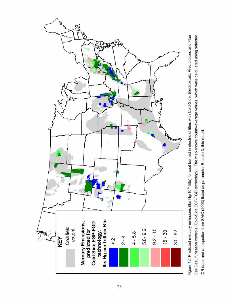
Fi

gure

12.

Pre

dict

ed m

ercu

ry e

mis

sion

s (lb

s H

g/10

12 B

tu) f

or c

oal b

urne

d in

ele

ctric

util

ities

with

Col

d-S

ide,

Ele

ctro

stat

ic P

reci

pita

tors

and

Flu

e

Gas

Des

ulfu

rizat

ion

cont

rols

(Col

d-S

ide

ES

P-F

GD

tech

nolo

gy).

The

map

sho

ws

coun

ty-a

vera

ge v

alue

s, w

hich

wer

e ca

lcul

ated

usi

ng s

elec

ted

ICR

dat

a, a

nd a

n eq

uatio

n fro

m S

AIC

(200

3) li

sted

as

para

met

er E

, tab

le 3

, thi

s re

port.

24

Coa

lfiel

d ex

tent

Mer

cury

Em

issi

ons,

pred

icte

d fo

rH

ot-S

ide

ESP

tech

nolo

gy,

lbs

Hg

per

trill

ion

Btu

< 2

2 - 4

4 - 5

.8

5.8

- 9.2

9.2

- 15

15 -

30

KEY

30 -

52

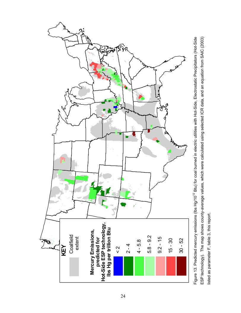
Figu

re 1

3. P

redi

cted

mer

cury

em

issi

ons

(lbs

Hg/

1012

Btu

) for

coa

l bur

ned

in e

lect

ric u

tiliti

es w

ith H

ot-S

ide,

Ele

ctro

stat

ic P

reci

pita

tors

(Hot

-Sid

e

ES

P te

chno

logy

). T

he m

ap s

how

s co

unty

-ave

rage

val

ues,

whi

ch w

ere

calc

ulat

ed u

sing

sel

ecte

d IC

R d

ata,

and

an

equa

tion

from

SA

IC (2

003)

liste

d as

par

amet

er F

, tab

le 3

, thi

s re

port.

25

Coa

lfiel

d ex

tent

Mer

cury

Em

issi

ons,

pred

icte

d fo

rH

ot-S

ide

ESP

- FG

D

tech

nolo

gy,

lbs

Hg

per t

rillio

n B

tu

< 2

2 - 4

4 - 5

.8

5.8

- 9.2

9.2

- 15

15 -

30

KEY

30 -

52

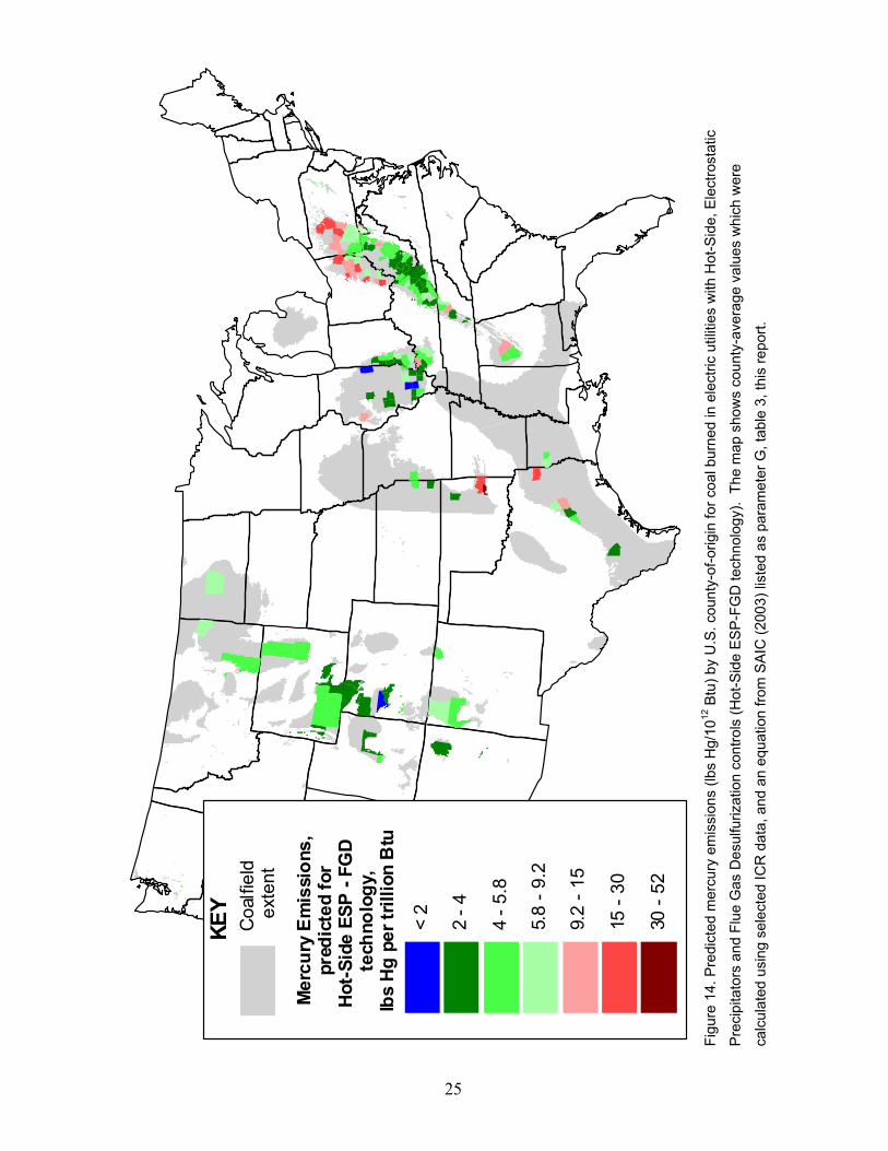
Fi

gure

14.

Pre

dict

ed m

ercu

ry e

mis

sion

s (lb

s H

g/10

12 B

tu) b

y U

.S. c

ount

y-of

-orig

in fo

r coa

l bur

ned

in e

lect

ric u

tiliti

es w

ith H

ot-S

ide,

Ele

ctro

stat

ic

Pre

cipi

tato

rs a

nd F

lue

Gas

Des

ulfu

rizat

ion

cont

rols

(Hot

-Sid

e E

SP

-FG

D te

chno

logy

). T

he m

ap s

how

s co

unty

-ave

rage

val

ues

whi

ch w

ere

calc

ulat

ed u

sing

sel

ecte

d IC

R d

ata,

and

an

equa

tion

from

SA

IC (2

003)

list

ed a

s pa

ram

eter

G, t

able

3, t

his

repo

rt.

26

Coa

lfiel

d ex

tent

Mer

cury

Em

issi

ons,

pred

icte

d fo

rSD

A -

FFte

chno

logy

,lb

s H

g pe

r tril

lion

Btu

< 2

2 - 4

4 - 5

.8

5.8

- 9.2

9.2

- 15

15 -

30

KEY

30 -

52

Fi

gure

15.

Pre

dict

ed m

ercu

ry e

mis

sion

s (lb

s H

g/10

12 B

tu) b

y U

.S. c

ount

y-of

-orig

in fo

r coa

l bur

ned

in e

lect

ric u

tiliti

es w

ith S

pray

-Dry

Ads

orpt

ion

and

Fabr

ic F

ilter

con

trols

(SD

A-FF

tech

nolo

gy).

The

map

sho

ws

coun

ty-a

vera

ge v

alue

s, w

hich

wer

e ca

lcul

ated

usi

ng s

elec

ted

ICR

dat

a, a

nd a

n

equa

tion

from

SA

IC (2

003)

list

ed a

s pa

ram

eter

H, t

able

3, t

his

repo

rt.

27

Coa

lfiel

d ex

tent

Mer

cury

Em

issi

on R

ate,

pred

icte

d fo

rco

ld-s

ide

ESP

- FG

Dte

chno

logy

,lb

s H

g pe

r TW

-h

< 6

6 - 2

0

20 -

40

40 -

62

62 -

100

100

- 221

KEY

Fi

gure

16.

Pre

dict

ed m

ercu

ry e

mis

sion

rate

(lbs

Hg/

tera

wat

t-hou

r, w

hich

is th

e sa

me

as lb

s H

g x

10-6

/meg

awat

t-hou

r) fo

r coa

l bur

ned

in e

lect

ric

utilit

ies

with

Col

d-S

ide,

Ele

ctro

stat

ic P

reci

pita

tors

and

wet

Flu

e G

as D

esul

furiz

atio

n co

ntro

ls (C

old-

Sid

e E

SP-F

GD

tech

nolo

gy).

The

map

sho

ws

coun

ty-a

vera

ge v

alue

s, w

hich

wer

e ca

lcul

ated

usi

ng s

elec

ted

ICR

dat

a ex

pres

sed

on a

net

ene

rgy

basi

s, a

nom

inal

hea

t rat

e of

35%

, and

an

equa

tion

from

SA

IC (2

003)

list

ed a

s pa

ram

eter

I, ta

ble

3, th

is re

port.

28

Coa

lfiel

d ex

tent

Mer

cury

Em

issi

on R

ate,

pred

icte

d fo

rSD

A -

FF

tech

nolo

gy,

lbs

Hg

per

TW-h

< 6

6 - 2

0

20 -

40

40 -

62

62 -

100

100

- 221

KEY

Figu

re 1

7. P

redi

cted

mer

cury

em

issi

on ra

te (l

bs H

g/te

raw

att-h

our,

whi

ch is

the

sam

e as

lbs

Hg

x 10

-6/m

egaw

att-h

our)

for c

oal b

urne

d in

ele

ctric

utilit

ies

with

Spr

ay-D

ry A

dsor

ptio

n an

d Fa

bric

Filt

er c

ontro

ls (S

DA

-FF

tech

nolo

gy).

The

map

sho

ws

coun

ty-a

vera

ge v

alue

s, w

hich

wer

e ca

lcul

ated

usin

g se

lect

ed IC

R d

ata

expr

esse

d on

a n

et e

nerg

y ba

sis,

a n

omin

al h

eat r

ate

of 3

5%, a

nd a

n eq

uatio

n fro

m S

AIC

(200

3) li

sted

as

para

met

er J

,

tabl

e 3,

this

repo

rt.

29

RESULTS AND DISCUSSION

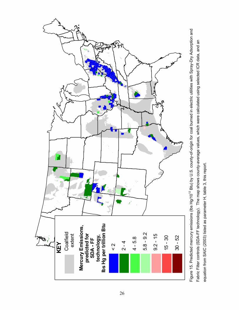
Draft maps showing the potential mercury and acid-gas emissions from coal combustion, by U.S.

county-of-origin were constructed using selected ICR coal quality data, and technology-specific

equations that predict mercury capture (SAIC, 2003). In this section we evaluate the coal assay

data that these maps are based on and conclude with a brief discussion of the significance and

limitations of the draft maps.

Evaluation of Coal Assay Data

Coal assay data used in this study include:

• 19,507 FERC 423 data records from 187 U.S. counties (USEIA, 2003a),

• 25,818 ICR data records from 169 U.S. counties (USEPA, 2003),

• 5,602 CTRDB data records from 116 U.S. counties (USEIA, 2003b),

• 5,045 COALQUAL data records from 340 U.S. counties (Bragg and others, 1997), and

• 73 PSU-DOE data records from 47 U.S. counties (Anonymous, 1990; Davis and Glick, 1993;

Scaroni and others, 1999).

The ICR data are the foundation of the draft maps (figures 8 to 17), whereas the COALQUAL,

FERC 423, CTRDB, and PSU-DOE data were used to estimate ICR moisture and hydrogen

values, and to verify these estimates and their derived values. Comparison of these data sets

shows data limitations, provides geochemical insights, and suggests mercury mitigation

strategies.

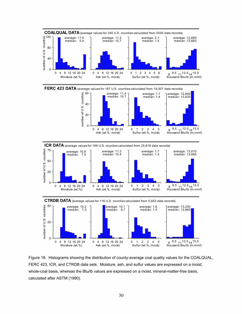
County-average, moisture, ash, sulfur, and Btu/lb values for four data sets are compared

in figures 18 and 19. Note that the data sets compared in figure 18 are populated by different

numbers of counties, whereas the comparisons shown in figure 19 only include counties that are

common to both the ICR, and the FERC 423, CTRDB, or COALQUAL data sets.

30

0 4 8 12 16 20 240

25

50

75

0 4 8 12 16 20 24 0 1 2 3 4 5

thousand Btu/lb (m,mmf)Sulfur (wt.%, moist)Ash (wt.%, moist)

0 4 8 12 16 20 240

40

80

120

0 4 8 12 16 20 24 0 1 2 3 4 5 6

0 4 8 12 16 20 240

20

40

60

0 1 2 3 4 5

0 4 8 12 16 20 240

25

50

0 4 8 12 16 20 24 0 1 2 3 4 5

average: 11.4median: 10.7


average: 12,940median: 13,620













ICR DATA (average values for 169 U.S. counties calculated from 25,818 data records)

FERC 423 DATA (average values for 187 U.S. counties calculated from 19,507 data records)

CTRDB DATA (average values for 116 U.S. counties calculated from 5,602 data records)

COALQUAL DATA (average values for 340 U.S. counties calculated from 5045 data records)

8 1411 15.512.59.5

8 1411 15.512.59.5thousand Btu/lb (m,mmf)Sulfur (wt.%, moist)Ash (wt.%, moist)Moisture (wt.%)



Figure 18. Histograms showing the distribution of county-average coal quality values for the COALQUAL,

FERC 423, ICR, and CTRDB data sets. Moisture, ash, and sulfur values are expressed on a moist,

whole-coal basis, whereas the Btu/lb values are expressed on a moist, mineral-matter-free basis,

calculated after ASTM (1990).

31

Figure 19. Cross-plots comparing the county-average moisture, ash, sulfur, and Btu values from the ICR

data set with those from the CTRDB, COALQUAL, and FERC 423 data sets; the Btu/lb values were

calculated after ASTM (1990).

32

Figures 18 and 19 show reasonably good agreement between the data sets, especially for

data corresponding to commercial coal shipments (FERC 423, CTRDB, and ICR). The

correlation between the ICR and FERC 423 sulfur values shown in figure 19 deserves comment.

Despite the good correlation, a few counties deviate from the 1:1 line. Many of these deviations

can be attributed to instances where the county-average values are calculated from one or two

data records. However a few instances may indicate potential bias in ICR data. Given that the

ICR data relied on periodic assays, and include a disproportionate number of records for small

(<50 MW) utilities, it is likely that the FERC 423 data better represent the quality of commercial

U.S. coal than the ICR data. Moreover, sulfur exhibits a positive correlation with mercury for

aggregated data (Quick and others, 2003). Consequently, instances where ICR sulfur is higher

than FERC 423 sulfur may indicate erroneously high county-average ICR mercury values.

Conversely, instances where the ICR sulfur is lower than the FERC 423 sulfur may indicate

erroneously low county-average ICR mercury values.

The larger number of counties included in the COALQUAL data set should be

considered when evaluating the data distributions shown in figure 18. For example, the

relatively high, average moisture value for the 340 counties listed in the COALQUAL data set

(figure 18) is a result of the comparatively large number of counties in the COALQUAL data set

with high-moisture (low-rank) coal. Thus, the relatively high average COALQUAL moisture

value shown in figure 18 is due to a geographic, rather than analytical, bias. Restricting the

comparison of moisture values to common counties (figure 19) shows that the COALQUAL

assay moisture values are actually relatively low. Although the relatively low COALQUAL

moisture values may relate to added moisture from washing of commercial coal (ICR and

CTRDB data), moisture loss prior to analysis of the COALQUAL coal samples is probably more

33

significant. Indeed, Bragg and others (1997) noted that the calculated ASTM rank for some

COALQUAL data records might be anomalously high due to air-drying of the samples before

analysis. The low COALQUAL moisture values due to assay bias are also consistent with the

relatively high, moist-basis COALQUAL Btu/lb values (figure 19).2

As noted earlier in this report, systematically low COALQUAL moisture values

complicate the evaluation of rank and the calculation of net heating values. Fortunately, the low

moisture values have little effect on COALQUAL emission factors expressed on an energy basis.

For example, the calculation of pounds sulfur per million Btu gives the same result regardless of

whether moist-basis sulfur and Btu/lb values, or dry-basis sulfur and Btu/lb values, are used for

the calculation. Figures 20 and 21 compare ICR sulfur, mercury, and chlorine values expressed

on an energy-basis to equivalent COALQUAL values.

2 As noted in an earlier report (Quick and others, 2004), it was necessary to adjust some COALQUAL assay values (notably Hg and Cl) for unmeasured residual moisture in the analysis specimen. This systematic bias was the result of the sample preparation method for inorganic assays, and is not related to the moisture bias described here (which, with few exceptions, only influences the proximate, ultimate, and sulfur form analyses).

34

0 1 2 3 4 50

50

100

0 1 2 3 4 50

50

100

0 10 20 30 40 500

50

100

0 60 120 1800

50

100

lbs Hg per tri l l ion Btu lbs Cl per bil l ion Btu

ICR DATA (average values for U.S. counties)

COALQUAL DATA (average values for U.S. counties)

average: 14 median: 12counties: 340

average: 11 median: 8

counties: 169



average: 1.9 median: 1.4counties: 340

average: 1.5 median: 1.2counties: 169

lbs S per mill ion Btu

lbs S per mill ion Btu0 10 20 30 40 50

0

50

100

0 60 120 1800

50

100

lbs Hg per tri l l ion Btu lbs Cl per bil l ion Btu

Figure 20. Distribution of county-average, mercury, chlorine and sulfur values for in-ground coal

(COALQUAL DATA) and commercial coal (ICR DATA).

a b c

ICR lbs Hg per tri l l ion Btu

+++

++++

+

++

++

+++++++ +++

+

+++++

+

+

+

+

+

+++

+

+

++++

+++

+

+

+++

++

+++

++ +

+

+

++ ++ +

+

+ ++

+ ++

+

++

+

+++

++

+ ++ ++

++

+++

+ ++

++

++

+++

+

+

+

++

+ + +

+

++

+

++

+ +

++

+++

+++

+

+++

+

+++++

+

++

+

+

+

+

0

20

40

0 20 40ICR lbs Cl per bil l ion Btu

++

+

+++

++

+ +

+

+

++

++

+

+

+

+

++

+

+

+

++

++

+

++

++

++ +

+

++++

++ +

+++

+

+++

++

++++++

+ + ++ ++

+++ ++

+

+

+ ++

++++

++

+

+++++

+

++

+ +++

+ ++++++ +

+

+0

100

200

0 100 200

++

+

++++ +++

++

+++++++

++

+++

+

+

+

++

++

+

+++

+++

+++

++++

+

++

++

+

++++

++

+

+++ +

+++

+

+

+++

+

+++++

++

+

+

+ ++ ++++

++++ ++ +

++

++

+++

+++++

++++

+

+ +

++

+

++++

+

+ +

+

+ +

+

+

+

+

++

++

++ +

+

+

++

++

0

2

4

6

0 2 4 6ICR lbs S per mill ion Btu

+ average value for a U.S. county

KEY1:1 line

Figure 21. Comparison of mercury, chlorine, and sulfur values in the ICR and COALQUAL data sets.

Data points show average values for U.S. counties common to both data sets.

35

When examining figures 20 and 21 it is useful to recognize that the COALQUAL data

indicate the quality of the in-ground coal resource, whereas the ICR data indicate the quality of

commercial coal produced during 1999. Differences between the COALQUAL and ICR data are

inevitable because the COALQUAL data include additional records for coal beds that are not

mined. Nonetheless, comparison of these data is instructive. Figure 20 shows higher sulfur and

mercury values for the COALQUAL data than the ICR data. Quick and others (2003) also

observed higher COALQUAL sulfur and mercury values, which they attributed to selective

mining of low-sulfur and low-mercury coal, as well as reduction of sulfur and mercury due to

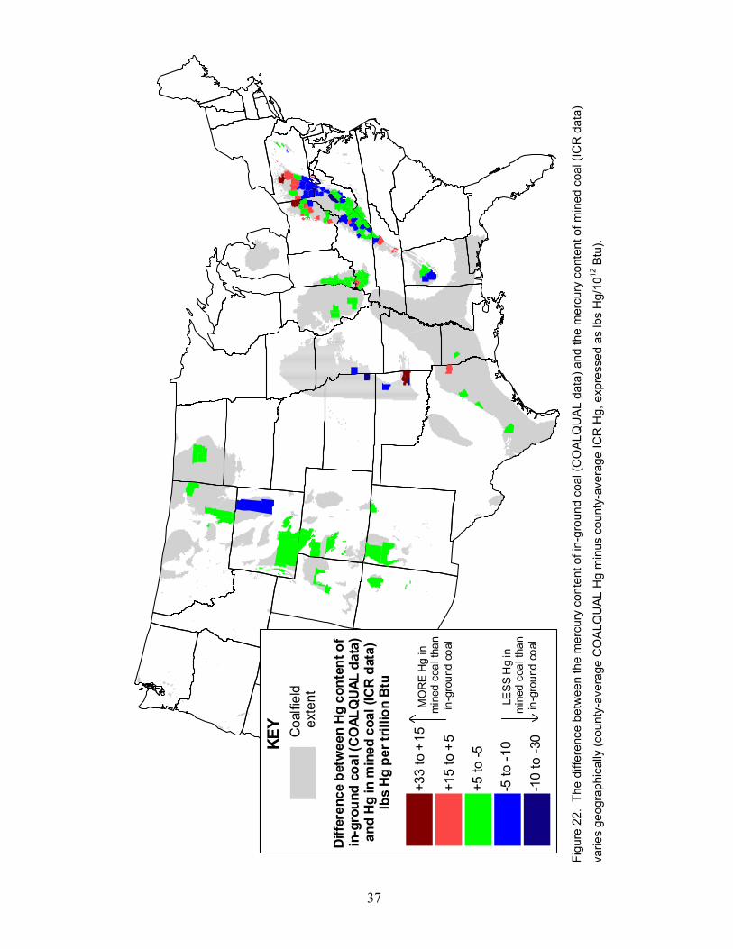
washing of mined coal. However, figure 21a shows that the mercury content of in-ground coal

(COALQUAL data) is not always lower than the mercury content of commercially shipped coal

(ICR data) when the comparison is restricted to coal from common counties-of-origin. Counties

where the mined coal contains more mercury than indicated by the COALQUAL data are

colored red in figure 22. The reason for the higher mercury content of coal mined in these areas

may be the combined result of limited washing, and contamination of mined coal by high-

mercury partings, roof rock, or floor rock; these contaminants are generally not included in

COALQUAL assay specimens because USGS sample collections guidelines (Swanson and

Huffman, 1976) require partings more than 5 mm thick to be excluded from the analysis sample.

Increased coal washing may be an effective Hg reduction strategy in instances where the ICR

mercury values are greater than the COALQUAL mercury values. Green areas on figure 22

show where mined coal contains substantially less Hg than the in-ground resource. Selective

mining and/or extensive coal washing probably explain these occurrences. For a few counties,

these differences may simply indicate bias in the ICR data (suggested by the different FERC 423

36

and ICR sulfur values, discussed above) or instances where the county average values are based

on only a few data records.

The different chlorine distributions for the COALQUAL and ICR data shown in figure 20

suggest preferential mining of counties with high-chlorine coal. However, such inferences are

uncertain given the limitations of the chlorine assays. For example, nearly 30% of the

COALQUAL chlorine values are reportedly below the assay detection limit (Bragg and others,

1997). Although only 14% of the selected ICR records are reportedly below the detection limit,

this is probably a minimum value. Nyberg (2003) notes that methods used to determine chlorine

concentrations in the ICR data collection effort were unreliable below 200 parts-per-million

(ppm or µg/g). Thirty percent of the selected ICR data records show dry chlorine at or below

200 ppm. Moreover, figure 23 shows that western U.S. counties are responsible for a

disproportionate share of the low-chlorine ICR data records.

37

Coa

lfiel

d ex

tent

Diff

eren

ce b

etw

een

Hg

cont

ent o

f in

-gro

und

coal

(CO

ALQ

UAL

dat

a)an

d H

g in

min

ed c

oal (

ICR

dat

a)lb

s H

g pe

r tril

lion

Btu

+33

to +

15

+15

to +

5

+5 to

-5

-5 to

-10

-10

to -3

0KEY

MO

RE

Hg

in

min

ed c

oal t

han

in-g

roun

d co

al

LES

S H

g in

m

ined

coa

l tha

nin

-gro

und

coal

Fi

gure

22.

The

diff

eren

ce b

etw

een

the

mer

cury

con

tent

of i

n-gr

ound

coa

l (C

OAL

QU

AL

data

) and

the

mer

cury

con

tent

of m

ined

coa

l (IC

R d

ata)

varie

s ge

ogra

phic

ally

(cou

nty-

aver

age

CO

ALQ

UA

L H

g m

inus

cou

nty-

aver

age

ICR

Hg,

exp

ress

ed a

s lb

s H

g/10

12 B

tu).

38

Coa

lfiel

d ex

tent

Chl

orin

e C

onte

ntpp

m C

l (dr

y)

< 20

0

200

- 600

600

- 1,0

00

1,00

0 - 1

,500

1,50

0 - 2

,500

> 2,

500

KEY

Figu

re 2

3. A

vera

ge c

hlor

ine

cont

ent o

f coa

l del

iver

ed to

U.S

. pow

er p

lant

s du

ring

1999

, by

coun

ty-o

f-orig

in (c

alcu

late

d us

ing

sele

cted

ICR

dat

a).

39

Evaluation of Technology-Specific Hg Emissions

Figures 11 to 17 show the predicted county-average mercury emissions for coal burned in

power plants classified by emission control technology. Note that these are draft figures and will

likely be modified. About 70% of existing coal-fired utility boilers rely on either hot-side or

cold-side ESP technology for emission control (Pavlish and others, 2003). Figures 11 and 13

show that eastern bituminous coal will rarely achieve the proposed MACT emission limit (2 lb

Hg/1012 Btu) for this substantial technology class. Likewise, no mercury compliance coals for

these power plants are indicated for western bituminous coal (this includes 100% of Arizona and

Utah production, 75% of Colorado production, and 38% of New Mexico production).

Conversely, county-average values for most western subbituminous coal are below the proposed

MACT limit (5.8 lb Hg/1012 Btu). Given the higher MACT limit proposed for subbituminous

coal compared to bituminous coal (table 1), switching to subbituminous coal may be an attractive

compliance option for western power plants with ESP emission controls.

Considering the proposed MACT limit for plants burning lignite (9.2 lb Hg/1012 Btu), the

results for Northern Great Plains or Gulf Coast lignite burned in ESP equipped power plants are

mixed. For example, in the Northern Great Plains, mercury compliance coal is indicated for

Oliver Co., North Dakota and Richland Co., Montana, whereas the more significant coal

production from McLean and Mercer Counties, North Dakota exceeds the proposed MACT

limit.

About 12% of U.S. coal-fired utility boilers use FGD technology (Pavlish and others,

2003). Figures 12 and 14 show that the addition of FGD technology reduces mercury emissions,

especially when combined with a cold-side ESP. Compared to ESP technology alone, there are

more examples of mercury compliance coal for power plants equipped with FGD technology.

40

However, despite better mercury capture using FGD, figures 12 and 14 show most bituminous

coal-producing counties still exceed the proposed MACT limit if burned in plants using ESP-

FGD emission controls.

Spray-dry-adsorption, fabric filter technology (SDA-FF) is used at about 4% of U.S.

coal-fired utility boilers. Figure 15 indicates mercury compliance for bituminous coal from most

counties when burned in power plants equipped with SDA-FF technology. However, the

performance of SDA-FF technology is unlikely to be as good as indicated. Mercury emissions

indicated by figure 15 are based on the county-average coal mercury and chlorine values, and the

mercury emission rate was calculated using equation H listed in table 4. Figure 24 shows that

the percent reduction of mercury emissions predicted by equation H (blue circles, SAIC 2003,

model 1) is greater than what is predicted by other model equations. Consequently, the SAIC

(2003) model is the most optimistic.

Although the different models for fabric filter technology shown in figure 24 clearly

differ, they all indicate greater than 90% mercury capture above 1,200 ppm chlorine, as well as

substantial sensitivity of predicted mercury capture when chlorine concentrations are below

about 200 ppm. The sensitivity of the models below 200 ppm chlorine has special significance

to western U.S. coal, given that the ICR chlorine assays are unreliable below this concentration

(Nyberg, 2003), and that western U.S. coal commonly contains less than 200 ppm chlorine

(figure 23).

41

••

•

•

•

•

•

•

••

•

•

•

•

•

•

•

•

•

•

••

•

•

•

•

•

•

•

••• •

•

••••• •

••

•

•

•• ••

•

••

•

•

•

•

•• ••••• •

••

•

•••

•••

•

•

•

•

•

•

•

•

•

••

•

•

•••

••

••••

•

•

•••

•

•••

••

••

• •• •• •

•

•

••• • ••

• •

•

•

• ••

•

•

•

•

•

•

•

•

•

•

•• ••••

•

•

•

•

•••

• ••

•• ••• •• •• •

•

•• •• •• •

•

•

•

•••

•

•

◊◊

◊

◊

◊◊

◊

◊◊◊◊

◊

◊

◊

◊

◊

◊

◊

◊

◊

◊

◊

◊◊

◊

◊

◊

◊

◊

◊◊

◊◊◊ ◊

◊

◊◊◊◊

◊◊

◊◊

◊

◊

◊

◊ ◊◊

◊

◊◊◊

◊

◊

◊

◊

◊ ◊◊◊◊◊

◊

◊◊◊

◊◊◊

◊◊◊

◊

◊

◊

◊

◊

◊◊

◊◊◊

◊◊

◊

◊

◊◊◊

◊

◊

◊◊◊

◊

◊

◊

◊◊

◊

◊

◊◊◊

◊

◊

◊

◊

◊◊◊ ◊◊ ◊

◊

◊

◊

◊◊◊ ◊◊

◊ ◊

◊

◊

◊ ◊◊

◊

◊

◊

◊

◊◊

◊

◊◊

◊

◊◊

◊

◊◊◊

◊

◊

◊

◊

◊◊

◊

◊ ◊

◊

◊◊ ◊◊◊

◊◊◊◊ ◊

◊

◊◊

◊◊ ◊◊ ◊

◊◊

◊

◊

◊◊◊◊

◊

••

•

•

•

•

•

••••

•

•

•

•

•

•

•

•

•

•

•

••

•

•

•

•

•

•

•

••• •

•

••

•••

•

••

•

•

•

•••

•

••

•

•

•

•

•

• •••••

•

••

•

•••

•••

•

•

•

•

•

••

•••

••

•

•

•••

•

•

•••

•

•

•

••

•

•

•••

•

•

•

•

•••

•• •

•

•

•

••

• ••

••

•

•

• ••

•

•

•

•

••

•

•

•

•

••

•

•••

•

•

•

•

••

•

• •

•

•••

•

•

••

•••

•

••

••

•• •

••

•

•

•••

••

∆∆

∆

∆

∆

∆

∆

∆∆∆∆

∆

∆

∆

∆

∆

∆

∆

∆

∆

∆

∆

∆∆

∆

∆

∆

∆

∆

∆∆

∆∆∆

∆

∆

∆∆∆∆

∆

∆

∆∆

∆

∆

∆

∆ ∆∆

∆

∆∆∆

∆

∆

∆

∆

∆ ∆∆∆∆∆

∆

∆∆

∆

∆∆∆

∆∆∆

∆

∆

∆

∆

∆

∆∆

∆∆∆∆∆

∆

∆

∆∆∆

∆

∆

∆∆

∆

∆

∆

∆

∆∆∆

∆

∆∆∆

∆

∆

∆

∆

∆∆∆

∆∆ ∆

∆

∆

∆

∆∆∆∆∆

∆∆

∆

∆

∆ ∆∆

∆

∆

∆

∆

∆

∆

∆

∆∆

∆

∆∆

∆

∆∆∆

∆

∆

∆

∆

∆∆

∆

∆ ∆

∆

∆∆ ∆∆

∆∆

∆∆

∆∆

∆

∆∆

∆∆

∆∆∆

∆∆

∆

∆

∆∆∆

∆∆

++

+

+

+

+

+

++++

+

+

+

+

+

+

+

+

+

+

+

++

+

+

+

+

+

++

+++

+

+

++++

+

+

++

+

+

+

+++

+

+++

+

+

+

+

+ ++++

++

++

+

+++

+++

+

+

+

+

++

++

+

++

+

+

+++

+

+

++

+

+

+

+

+++

+

+++

+

+

+

+

+++

++

+

+

+

+

++

+++

++

+

+

++

+

+

+

+

+

+

+

+

++

+

+

+

+

+++

+

+

+

+

+

+

+

++

+

+++

+

+

++

++

+

+

++

+

+++

+

++

+

+

+++

+

+

0

20

40

60

80

100

0 200 400 600 800 1,000 1,200

• SAIC (2003) SDA/FF model 1

◊ AEMS (2004) NMA FF model

• SAIC (2003) SDA/FF model 2

∆ ENSR (2003) West Associates SDA/FF model

+ Robertson (2002) EPRI SDA/FF model

Chlorine (ppm, dry)

= 1- exp[10.711- 1.2263Ln(lbsCl/1012Btu)]n = 10r2 = 0.89

= 1- exp[-0.446- 3.042E-5(lbsCl/1012Btu)]n = 16r2 = 0.60

= 1- exp[-0.0192- 3.1418E-5(lbsCl/1012Btu)]n = 10r2 = 0.87

= 1- 0.8188exp[-0.002164Clppm, dry]n = 10r2 = 0.94

= 0.2854Ln(Clppm, dry) - 1.1302n = 11r2 = 0.91

Figure 24. Five model equations predict increasing mercury capture by fabric filter emission controls with

increasing coal chlorine concentration. Note that the SAIC (2003) model 1 equation was used to predict

emissions in figures 15 and 17 of this report. Data points show county-average ICR chlorine values - and

their variously predicted mercury capture efficiencies - for 184 U.S. counties; not shown are 46 U.S.

counties where the average chlorine concentration is more than 1,200 ppm.

CONCLUSIONS

Draft maps showing potential sulfur, chlorine, and mercury emissions for U.S, coals by

county-of origin, show the following:

• As generally known, high-sulfur coal is produced in the Northern Appalachian

Region, as well as Eastern Interior, Western Interior, and Gulf Coast provinces,

whereas low-sulfur coal is produced from the Central Appalachian Region and the

western U.S.

42

• High-mercury coal is produced in parts of Oklahoma, Texas, Ohio, Pennsylvania,

Kentucky, Alabama, and Tennessee, whereas low-mercury coal is common in the

western U.S., Eastern Interior Province, and the Central Appalachian Region.

• Coal from the Northern Appalachian Region (Ohio and parts of Pennsylvania) has

notably high mercury concentrations, compared to other U.S. coal.

• Western U.S. coal typically contains less than 200 ppm chlorine, whereas eastern

U.S. coal generally contains more than 600 ppm chlorine.

• Much subbituminous and some lignite coal should comply with the proposed MACT

rule using existing technology. Bituminous compliance coal for power plants with

ESP controls is rare. Plants equipped with FGD controls may find bituminous

compliance coal in some western U.S. counties, the Eastern Interior Province, and the

Central Appalachian Region. With notable exceptions (for example, certain counties

in Ohio, Alabama, and the western U.S.), fabric filter technology may be an effective

technology for most bituminous coal.

REFERENCES

AEMS, LLC, 2004, Review and critique of data and methodologies used in the USEPA proposed

utility mercury MACT rulemaking, report prepared for the National Mining Association:

AEMS, LLC, Arlington Virginia, and RWCrawford Energy, Tuscon Arizona, 88 p.,

Online, <nma.org/pdf/pol_briefs/mact_critique_072004.pdf>, accessed July 2004.

43

American Society for Testing and Materials, 1990, D 388-90 Standard classification of coals by

rank, Annual Book of ASTM Standards: West Conshohocken, Pennsylvania, v. 05.05, p.

193-197.

— 2000a, D 3180-89 Standard practice for calculating coal and coke analyses from as-

determined to different bases, Annual Book of ASTM Standards: West Conshohocken,

Pennsylvania, v. 05.06, p. 252-255.

— 2000b, D 5373-93 Standard test methods for instrumental determination of carbon, hydrogen,

and nitrogen in laboratory samples of coal and coke, Annual Book of ASTM Standards:

West Conshohocken, Pennsylvania, v. 05.06, p. 453-456.

Anonymous, 1990, The Penn State Coal Sample Bank and Data Base, second edition: Coal and

Organic Petrology Laboratories, University Park, Pennsylvania, The Pennsylvania State

University, unpaginated data sheets.

Belyaev, S.S., Yy-Lein, A., and Ivanov, M.V., 1980, Role of methane-producing and sulfate-

reducing bacteria in the destruction of organic matter, in Trudinger, P.A., and Walter,

M.R., editors, Biogeochemistry of ancient and modern environments: Proceedings of the

Fourth International Symposium on Environmental Biogeochemistry (ISEB) and

Conference on Biogeochemistry in Relation to the Mining Industry and Environmental

Pollution (Leaching Conference), 26 August to 4 September, 1979, Canaberra, Australia:

Australian Academy of Science, p. 235-242.

Bragg, L.J., Oman, J.K., Tewalt, S.J., Oman, C.L., Rega, N.H., Washington, P.M., and

Finkelman R.B., 1997, Coal quality (COALQUAL) database – version 2.0: U.S.

Geological Survey Open-File Report 97-134, CD-ROM.

Chu, P., Goodman, N., Behrens, G., and Roberson, R., 2000, Total and speciated mercury

emissions from coal-fired power plants: Palo Alto, California, Electric Power Research

Institute, 15 p., Online, <epri.com/attachments/262300_EUEC_pchu_1-01.pdf>, accessed

July 2004.

Cole, J., 2003, MACT floor unit conversion from input-based standard to output-based standard

in the proposed national emission standards for hazardous air pollutants; and, in the

alternative, proposed standards of performance for new and existing stationary sources –

44

electric utility steam generating units, memorandum to Bill Maxwell, U.S. USEPA

OAQPS (C439-01): RTI International, 2 p., Online,

<epa.gov/ttn/atw/utility/mact_unit_conv_011504.pdf> accessed July 2004.

Davis, A., and Glick, D.C., 1993, Establishment and maintenance of a coal sample bank and data

base, final report to the U.S. Department of Energy for contract DE-RP22-87PC79997:

University Park, The Pennsylvania State University, Coal and Organic Petrology

Laboratories, 266 p.

ENSR Corporation, 2003, Multivariable method to estimate the mercury emissions of the best-

performing coal-fired utility units under the most adverse circumstances which can

reasonably be expected to recur; report DC\566987.6 prepared for WEST Asscociates,

Tucson, Arizona, and present at the March 4, 2003 meeting of the Clean Air Act

Advisory Committee Permits/New Source Review/Air Toxics Subcommittee Utility

MACT Working Group: 45 p., Online,

<epa.gov/ttn/atw/combust/utiltox/final_ensr_multivar.pdf>, accessed July 2004.

Gorbaty, M.L., and Kelemen, S.R., 2001, Characterization and reactivity of organically bound

sulfur and nitrogen in fossil fuels: Fuel Processing Technology, v. 71, p. 71-78.

Houghton, J.T., Meira Filho, L.G., Lim, B., Tréanton, K., Mamaty, I., Bonduki, Y., Griggs, D.J.,

and Callander, B.A., 1997, Greenhouse Gas Inventory Reference Manual, Revised 1996

IPCC Guidelines For National Greenhouse Gas Emissions (chapter 1, volume 3):

Geneva, Switzerland, World Meteorological Organization, Intergovernmental Panel on

Climate Change, 145 p.

Juniper, L., 1998, Competitiveness of Queensland thermal coals in the export market, Ultra-

Systems Technology Pty Ltd Report C1044 for the Queensland Department of Mines and

Energy: Brisbane, Australia, 57 p.

Maes, I.I., Gryglewicz, G., Machnikowska, H., Yperman, Y., Franco, D.V., Mullens, J., and Van

Pouke, L.C., 1997, Rank dependence of organic sulfur functionalities in coal: Fuel, v. 76,

p. 391-396.

Maxwell, W.H., 2003, Analysis of variability in determining MACT floor for coal-fired electric

utility steam generating units; memorandum to utility MACT files: U.S. Environmental

45

Protection Agency, 66 p., Online, <epa.gov/ttn/atw/utility/floor_dv_112603.pdf>,

accessed July 2004.

Nyberg, C., 2003, Quantitative determination of chlorine in lignite and subbituminous coals,

Center for Air Toxic Metals Newsletter: Grand Forks, University of North Dakota,

Energy and Environmental Research Center, v. 9, issue 2, p. 6 and 8.

Pavlish, J.H., Sondreal, E.A., Mann, M.D., Olson, E.S., Galbreath, K.C., Laudal D.L., and

Benson, S.A., 2003, Status review of mercury control options for coal-fired power plants:

Fuel Processing Technology, v. 82, p. 89-165.

Quick, J.C., Brill, T.C., and Tabet, D.E., 2003, Mercury in US coal – observations using the

COALQUAL and ICR data: Environmental Geology, v. 43, p. 247-259.

Quick, J.C., Tabet, D.E., Wakefield S., and Bon, R.L., 2004, Optimizing technology to reduce

mercury and acid gas emissions from electric power plants, semi-annual report, August

2003 to January 2004, for U. S. Department of Energy contract DE-FG26-03NT41901:

Salt Lake City, Utah Geological Survey, 49 p.

Roberston, R., 2002, UARG variability analysis, memorandum to Bob Wayland, U.S.

Environmental Protection Agency, presented at the October 17, 2002 meeting of the

Clean Air Act Advisory Committee Permits/New Source Review/Air Toxics

Subcommittee Utility MACT Working Group: Raleigh, North Carolina, RMB Consulting

and Research, 4 p., Online, <epa.gov/ttn/atw/combust/utiltox/epavarifnl.doc>, accessed

July 2004.

Robinson, J.M., 1990, Lignin, land plants and fungi – Biological evolution affecting Phanerozoic

oxygen balance: Geology, v. 15, p. 607-610.

Scaroni, A.W., Davis, A., Glick, D.C., Hatcher, P.G., Mitchell, G.D., Carson, D., and Lei, H.,

1999, Maintenance of the coal sample bank and data base; final technical report for the

U.S. Department of Energy contract DE-AC22-93PC93051: University Park, The

Pennsylvania State University, Coal and Organic Petrology Laboratories, 192 p.

Science Applications International Corporation, 2003, Calculation of possible mercury MACT

floor values for coal-fired utilities - influence of variability and approach; report for the

U.S. Department of Energy: Reston, Virginia, SAIC Corp., 46 p., 8 appendices, Online,

46

<netl.doe.gov/coal/E&WR/mercury/pubs/DOE_Report_v120803.pdf >, accessed August

2004.

Sinninghe Damste, J.S., Rijpstra, W.I.C., Kock-Van Dalen, A.C., deLeeuw, J.W., and Schenk,

P.A., 1989, Quenching of labile functionalized lipids by inorganic sulfur species -

evidence for the formation of sedimentary organic sulfur compounds at the early stage of

diagenesis: Geochimica et Cosmochimica Acta, v. 53, p. 143-155.

Swanson, V.E., and Huffman, C. Jr., 1976, Guidelines for sample collecting and analytical

methods used in the U.S. Geological Survey for determining chemical composition of

coal: U.S. Geological Survey Circular 735, 11 p.

Trumbell, J.V.A., 1960, Coal fields of the United States, exclusive of Alaska – sheet 1: U.S.

Geological Survey Map, scale 1:5,000,000, Online, <nationalatlas.gov/coalfdm.html>,

accessed February 2004.

U.S. Energy Information Administration, 2003a, Form FERC 423 Database, Monthly cost and

quality of fuels for electric power plants: Online,

<eia.doe.gov/cneaf/electricity/page/ferc423.html>, accessed October and November

2003.

—2003b, The Coal Transportation Rate Database data tables: Online,

<eia.doe.gov/cneaf/coal/ctrdb/database.html>, accessed October and November 2003.

U.S. Environmental Protection Agency, 2003, Unified air toxics website, electric utility steam

generating units hazardous air pollutant emission study: Online,

<epa.gov/ttn/atw/combust/utiltox/utoxpg.html>, accessed October and November 2003.

— 2004, Proposed national emission standards for hazardous air pollutants; and, in the

alternative, proposed standards of performance for new and existing stationary sources -

electric utility steam generating units; proposed rule: Federal Register, v. 69, no. 20, p.

4652-4752, Online, <epa.gov/ttn/atw/utility/frnotice_013003.pdf>, accessed July 2004.

Documents

OPTIMIZING TECHNOLOGY TO REDUCE MERCURY AND ACID GAS EMISSIONS