Optimum Design of Control Devices for Safe Seepage under Hydraulic

Journal of Engineering and Development, Vol. 10, No.1, March (2006) ISSN 1813-7822

66

Optimum Design of Control Devices for Safe Seepage under Hydraulic Structures

Abstract

The research aimed at determining the optimal control device in order to

decrease seepage under hydraulic structures. The finite-element method is used to

analyze seepage through porous media below hydraulic structures with blanket, cut-

off, or filter trench as seepage control devices. The effect of length and location of

the control devices is investigated.

The formulated optimization model is applied to a hypothetical case study. The

optimization problem is solved by the Lagrange-multiplier method to find the

minimum costs of control devices with safe exit gradient and uplift pressure.

For a hydraulic structure with different control devices, the minimum total cost

has been achieved when using a filter trench, while the maximum total cost was

when a downstream cut-off is used.

ةــــلاصـالخيهدف البحث إلى تحديد وسيلة السيطرة المثلى لتقليل الرشح تحت المنشآت الهيدروليكية. جرى استخدام طريقة العناصر المحددة لتحليل الرشح خلال الأوساط المسامية تحت المنشآت الهيدروليكية بوجود بطانة، جدار

تحرّي تؤثير طول وموقع تلك الوسائل لتحديد الطول قاطع، أو خندق مرشِح كوسيلة للسيطرة على الرشح، وتمّ والموقع الأمثلين.

لقد تمّ تطبيق نموذج الأمثلية المُصاغ على حالة تطبيقية افتراضية، وجرى حلّ المسؤلة بطريقة معامل Exit gradientلاكرانج لإيجاد الكلفة الأدنى لوسيلة السيطرة مع المحافظة على كل من انحدار المخرج

ضمن الحدود الآمنة. Uplift pressureضغط الرفع ولقد بيّن البحث أن الكلفة الكليّة الأدنى تكون باستعمال خندق مرشِح بينما كانت الأعلى عند استعمال جدار

قاطع عند المإخر.1. Introduction

Asst. Prof. Dr. Abdulhadi A. Al-Delewy

Civil Eng. Dept., College of Engineering

University of Babylon, Hilla, Iraq

Asst. Prof. Dr. Abdul-Hassan K. Shukur

Civil Eng. Dept., College of Engineering


Eng. Waked H. AL-Musawi

M.Sc. in Civil Engineering



67

Optimum use of water nowadays cannot be overemphasized. Hydraulic structures are a

specific type of engineering structures designed and executed in order to utilize it to control

water and ensure the aforementioned objective. The hydraulic structures represent the

important part of any flow network. Examples of such structures are dams, regulators, weirs,

… etc. The basic aim of these structures is to control the flow discharge and water levels.

The foundation of any hydraulic structure should be given the greatest importance in

analysis and design as compared with other parts of the structure, because failure in the

foundation would destroy the whole structure.

One of the most important problems that causes damage to hydraulic structures is

seepage under the foundations, which occurs due to the difference in water level between the

upstream, (U/S), and downstream, (D/S), sides of the structures. The water seeping

underneath the hydraulic structure endangers the stability of the structure and may cause

failure.

Water seeping under the base of a hydraulic structure starts from the U/S side and tries

to emerge at the D/S end of the impervious floor. If the exit gradient is greater than the critical

value for the foundation, a phenomenon called piping may occur due to the progressive

washing and removal of the fines of the subsoil [1]

. Moreover, the uplift force which occurs as

a result of the water seeping below the structure exerts an uplift pressure on the floor of the

structure. If this pressure is not counterbalanced by the weight of the floor, the structure may

fail by rupture of a part of the floor.

The problems of piping and uplift are practically tackled through a variety of methods of

seepage control, aiming at ensuring the safety of the respective structure and at the same time

saving the possibly-seeping water. The common provisions in this respect are:

1. Upstream blanket.

2. Upstream or/and downstream cut-offs.

3. Subsurface drain on the downstream side.

4. Filter trench on the downstream side.

5. Weep holes, or pressure relief wells on the downstream side.

This research aims at determining the optimal control device to decrease seepage under

hydraulic structures.

2. Review of Literature

There are different methods to find the piezometric head distribution under hydraulic

structures from which the hydraulic gradient is computed. As a result of the difficulties which

were met through empirical and analytical methods, it was resorted to numerical methods.

Such methods provide obtaining the required results with a good accuracy such that they are

well comparable to the results of the analytical solutions.

Conner and Brebbia [2]

, solved the seepage problem under a hydraulic structure with two

piles resting on isotropic soil by using a finite element method in order to find the distribution

of pressure under the base of the structure.


68

Cechi and Mancino [3]

and Zienkiewicz [4]

have given application examples of simple

cases for seepage under hydraulic structures by using triangular grid of finite element to find

the head distribution under the structures.

Nassir [5]

applied the finite element method in a wider range. He analyzed the seepage

problems under hydraulic structures by using different shapes of the finite elements in order

to choose the best solution that gives the most exact results.

Hatab [6]

and Ijam and Hatab [7]

used the finite element method in the analysis of

seepage through homogeneous and isotropic porous media below hydraulic structures with

horizontal filters. They also studied the stability of the structures with vertical drains.

Ijam and Nassir [8]

used the finite element method to study seepage under hydraulic

structures for isotropic soil with two cut-offs.

Khsaf [9]

used the finite element method to analyze seepage in isotropic, anisotropic,

homogeneous and non-homogeneous soil foundations underneath hydraulic structures

provided with flow control devices.

Gill [10]

used the theoretical ideas presented by Bennett [11]

criteria for optimal design of

rectangular, triangular, and trapezoidal blankets.

Hamed [12]

used Rosenbrock constrained optimization and sequential unconstrained

minimization technique to solve the non-linear programming problem to find the optimum

design of barrage floor (area of concrete and reinforcement).

3. The Finite-Elements Scheme

Real groundwater flow, in general, is a three-dimensional, unsteady, laminar flow of a

practically-incompressible fluid (the water), through a heterogeneous and anisotropic

medium. However, most of the problems of seepage analysis beneath hydraulic structures are

usually simplified by assuming a two-dimensional, steady flow through a homogeneous and

isotropic medium.

Flow through a saturated porous medium is generally governed by Darcy’s law [13]

. The

governing equation for such a flow is obtained by joining Darcy's law with the equation of

continuity. With the aforementioned simplifications, the governing equation for such a flow

would be :

Substituting Darcy’s Law in the continuity equation for three-dimensional, steady, and

incompressible flow results in:

0y

h

x

h2

2

2

2

………………………………………………………………... (1)

where: (h) is the piezometric head, (L); (x) and (y) are the horizontal and vertical Cartesian

coordinates, respectively.

Thus, the seepage pattern can be completely determined by solving Eq.(1), subject to the

boundary conditions of the flow domain.


69

For the steady state of a confined flow, the boundary conditions are defined as follows:

1. Reservoir Boundaries

The water depth (ho) above such boundaries is always known; so, the pressure (p) at any

point on these boundaries would be:

ow hp ……………………………………………………………………. (2)

Therefore, the piezometric head distribution along the reservoir boundaries (S1) is

constant; that is:

zp

hhw

o

………………………………………………………………... (3)

For this reason, all the reservoir boundaries are equipotential lines.

2. Impervious Boundaries

At impervious boundaries, (S2), the water cannot seep through the surface. Thus, the

velocity component normal to the boundary, (Vn), must be equal to zero. That is:

0Ly

hkL

x

hkV yyxxn

………………………………………….. (4)

where: (Kx) and (Ky) are the hydraulic conductivities of the aquifer in the (x) and (y)

directions, respectively, [however, for an assumed isotropic aquifer then (Kx = Ky = K), where

(K) is the average hydraulic conductivity of the aquifer]; (Lx) and (Ly) are the direction

cosines of the normal vector on the surface with the directions (x) and (y), respectively. These

boundaries represent streamlines of constant stream functions.

Figure (1) illustrates the boundary conditions of a typical problem of seepage under a

hydraulic structure.

The basic idea of the finite element method is to discretize the problem domain to

sub-domains or finite elements. These elements may be one, two, or three-dimensional and

joined to each other by nodes existing on element boundaries; the nodes are regarded as part

of the element. After the discretization process, the behavior of the field variable on each

element is represented approximately by a continuous function depending on nodal values of

the field variable as follows:

n

1i

ii

e hNh ………………………………………………………………….. (5)

where:


70

Gate Floor base ho

Reservoir Boundary (S1) Reservoir Boundary (S1)

Soil foundation

Impervious

boundary(S2) (S2)

Impervious

boundary(S2) (S2)

Impervious

boundary(S2) 2)(S2)

Upstream water

level

he = approximate solution for piezometric head distribution in the element (e), (L);

N = shape function of the element (e) ; hi = nodal values of head of the element (e), (L);

n = number of nodes in the element (e).

Substituting Eq.(5) in Eq.(1) gives:

0RhNy

ky

hNx

kx

en

1i

iiy

n

1i

iix

…………………………… (6)

where: Re = element residual.

Figure (1) Boundary Conditions of a Typical Problem of Seepage under a Hydraulic Structure

The best solution is the one which makes this residual a minimum or maintains it small

at all points of the domain. In order to reach this aim, Eq.(6) should be integrated on the

problem domain after weighting by a certain function and should equal zero as follows:

e

e

n

1A

e

j 0AdRW ………………………………………………………….. (7)

where: Wj = weighted function.


71

There are different approaches which can be used, depending on the choice of the

weighted function. The best is the one which is known as Galerkin technique where the

weighted function is taken equal to the shape function (i.e., Wj = Nj) [14]

.

Then substituting Eq.(6) in Eq.(7) yields:

0dAhNy

ky

hNx

kx

Nne

1 A

n

1i

iiy

n

1i

iix

e

je

………………….. (8)

where: dA = dx .dy; (j=1, 2, …, n); n = number of nodes for each element.

To reduce continuity requirements for the shape function, (N), from (C1-continuity) to

(Co-continuity), integration by parts with Green’s theorem is applied to the second order

derivatives terms, where (C1) and (C

o) are the continuity for the shape function for the first

and zero stage, respectively [15]

.

Accordingly, the first term of Eq.(8) will be:

e eA

n

1

iixA

e

j

S

n

1

iix

e

j

n

1

iix

e

j dAhNx

kx

NdyhN

xkNdAhN

xk

xN ….. (9)

The second term of Eq. (8) will be:

e eA

n

1

iiyA

e

j

S

n

1

iiy

e

j

n

1

iiy

e

j dAhNy

ky

NdxhN

ykNdAhN

yk

yN … (10)

Substituting Eqs.(9) and (10) in Eq.(8) results in:

e

e

n

1S

n

1

iinjA

n

1

iiy

jn

1

iix

jdshN

nkNdAhN

yk

y

NhN

xk

x

N … (11)

where: ( e

2

e

1 SSS ) represents the surface boundaries of the element.

Then applying the boundary conditions in Eq. (11) gives:

0dsLhNy

kNLhNx

kN

dydxhNy

ky

NhN

xk

x

N

e1

e

e

S

n

1

yiiyj

n

1

xiixj

n

1A

n

1

iiy

jn

1

iix

j

…………………….. (12)


72

x

y

7 6 5

8 4

1 2 3

and in matrix form:

0hKen

1

i

e ………………………………………………………………... (13)

where: [Ke] represents the element matrix:

eA

eeTee 0dydxBDBK …………………………………………….. (14)

where:

y

N

y

N

y

N

x

N

x

N

x

N

Be

n

e

2

e

1

e

n

e

2

e

1

e

y

xe

k0

0kD

and from assemblage:

[K] {h} = 0 …………………………………………………………………… (15)

where, [K] is the global matrix = eK

The assembled equation, Eq.(15), is solved using a frontal solution because of its

efficiency in computer storage requirement [16]

.

In the present work, two-dimensional quadratic Isoparametric elements are used which

have eight nodes, as shown in Fig.(2).

Figure (2) A Quadratic Isoparametric element


73

From the value of the piezometric head at the nodes, it is possible to compute the

hydraulic gradient directly without the need for transformation. That is:

8..,,.2,1ihNh ii

882211 hN...hNhNh ………………………………………………. (16)

Therefore, x

h

and

y

h

can be written as follows:

88

22

11

88

22

11

hy

N...h

y

Nh

y

N

y

h

hx

N...h

x

Nh

x

N

x

h

………………………………………... (17)

In matrix form, the above equation becomes:

8

2

1

821

821

h

h

h

y

N

y

N

y

N

x

N

x

N

x

N

y

h

x

h

……………………………………... (18)

or:

8

2

1

821

821

1

h

h

h

NNN

NNN

J

y

h

x

h

………………………………… (19)

where: [J] is the Jacobian matrix.

The solution of Eq.(19) will give the hydraulic gradient in the x and y-directions.

4. The Optimization Problem

The purpose of optimization is to find the best possible solution among the many

potential solutions satisfying the chosen criteria. Designers often base their designs on the

minimum cost as an objective, taking into account mainly the costs of foundation, safety, and

serviceability.


74

A general mathematical model of the optimization problem can be represented in the

following form:

A certain function (Z), called the objective function,

Z = f {xi} I = 1, 2, …, n …………………………………………… (20)

which is usually the expected benefit (or the involved cost), involves (n) design variables {x}.

Such a function is to be maximized (or minimized) subject to certain equality or inequality

constraints in their general forms:

iii bxg ; i =1, 2, …, I …………………………………………... (21)

jjj bxq ; j =1, 2, …, J …………………………………………... (22)

The constraint reflects the design and functional requirements. The vector {x} of the

design variables will have optimum values when the objective function reaches its optimum

value.

Of the many optimization techniques available, the formulated problem lends itself as a

nonlinear model.

4-1 Design Variables

The design variables are taken as follows [see Fig.(3)]:

1. Difference head (H): (2, 4, 6, 8, 10, 12 and 14m).

2. Length of floor (b): 3 m b < 50 m.

3. Thickness of the floor base (t): Calculated by Eq.(24).

4. Length of upstream blanket (b1): Calculated from the floor length value in order to avoid

the uplift pressure and critical exit gradient.

5. Depth of the upstream cut-off (d1): 0 – 12 m; step 0.5 m.

6. Depth of the downstream cut-off (d2): 0 – 12 m; step 0.5 m.

7. Filter trench: with filter and without filter.


75

U/S

side =

10

0 m

H

b1

d1

d2

t/3

b/3

b

/3

b/3

t/3

24

m

t

Flo

or len

gth

(b)

D

/S sid

e = 1

00

m

Figure (3) Illustrative Sketch of a Hypothetical Case Study


76

4-2 The Objective Function

The cost objective function (Z) of the present research involves the cost of both floor

and any control device. Such a function is formulated as follows:

z.wcbcdcdcacZ 41322121 …………………………………….. (23)

where:

c1 = cost of one cubic meter of the floor base material, (106 I.D. / m

3);

a = area of floor base, (m2);

c2 = cost of one square meter of cut-off, (106 I.D. / m

2);

d1 ,d2 = depths of upstream and downstream cut-offs, respectively, (m);

c3 = cost of one square meter of upstream blanket, (106 I.D. / m

2);

b1 = length of upstream blanket, (m);

c4 = cost of one cubic meter of the filter trench, (106 I.D. / m

3);

w = width of filter trench, (m); and

z = depth of filter trench, (m).

4-3 Constraints

The objective function is to be minimized, subject to the following constraints:

1. The ratio of the length of any control device used to the length of floor base for a certain

differential head (H) should be such that a safe exit gradient (used as 0.25 in this research)

will be ensured.

2. The floor thickness, with any control device used, shall be limited to a certain value to help

in counteracting the uplift water pressure. This requirement is stated as follows:

For equilibrium: Uplift pressure = Downward pressure; that is: w(h+t) = w.Gc.t or:

1G

ht

c …………………………………………………………………….. (24)

where:

t = thickness of floor base under the gates , (L);

h = head at any point under the hydraulic structure, (L);

Gc = specific gravity of concrete (the floor material) = 2.4; and

w = unit weight of water, (F/L3).

3. The cut-off depth should be equal to or less than (12 m).

4-4 Method of Optimization

The method of optimization employed in this research is the Lagrange multiplier

method. The Lagrangian would be:


77

2

j

m

1ij

jj

m

1i

ii xqxgxFL

…………………………….. (25)

where: (m) denotes the total number of constraint equations, (1, 2, …, m) are the Lagrange

multipliers, and(θ) is a dummy variable. The Lagrangian involves the original (n) variables

plus (m) number of (λ) variables and a similar number of (θ) variables, making a total of

(n+2m) unknowns.

Differentiating the Lagrangian with respect to each of the stated unknowns, one at a

time, and equating each formulated derivative to zero (for the minimization goal) will yield

(n+2m) equations as follows:

0x

q

x

g

X

F

x

L

j

jm

11j

j

i

im

1i

i

jj

…………………………………….. (26)

0gL

i

i

………………………………………………………………… (27)

02L

jj

j

…………………………………………………………….. (28)

Solving Eqs. (26), (27), and (28) simultaneously gives the required optimal solution.

5. Analysis of the Results

In this research, different cases were analyzed to investigate the effect of length and

location of control devices (blanket, cut-off, and filter trench) on uplift pressure and exit

gradient by using the finite-element method. Figure (4) shows the discretization mesh of the

finite-elements of a hydraulic structure with an upstream blanket (b1), downstream blanket

(b2), upstream cut-off (d1), downstream cut-off (d2), and filter trench.

In order to determine the optimum design of control devices, many cases were examined

using the Lagrange multiplier method and cost calculation curves with various values of

active head (H). For this purpose, the difference ratio of piezometric head is considered, that

is:

21

2*

hh

hhH

…………………………………………………………………... (29)

where:

H* = ratio of head difference;

h = piezometric head at any point in the flow domain, (L);

h1, h2= piezometric head (U/S) and (D/S) of the structure, respectively, (L).

Consequently, (H*) equals (one) for the upstream bed and (zero) for the downstream bed.


78

d1

z

w

Filter trench

(H*=0) H

h2 H*=0 b2

b/3 b1

A

B

H*=1.0

h1

T=2b

U/S side = 1.5b b D/S side = 1.5b

c

x x

Figure (4) The Finite Element Mesh Discretization of a Hydraulic

Structure with U/D Blankets, U/S Cut-Off, and Filter Trench


79

Figure (5) shows the effect of using an upstream or downstream blanket on the uplift

pressure. It has been noted that the uplift pressure is decreased when using an upstream

blanket, as compared with the case without blanket, other parameters being unchanged. Also,

the uplift pressure increases with using a downstream blanket. The same aforementioned

effect can be noticed on the exit gradient and as it is shown in Fig.(6).

0.0 0.2 0.4 0.6 0.8 1.0Distance along floor base (x/b)

0.0

0.2

0.4

0.6

0.8

1.0

without blanket

U/S blanket

D/S blanket

b /b=0.5

H*

1,2

Figure (5) The Effect of using the U/S or D/S Blanket on the Uplift Pressure

0.0 0.3 0.6 0.9 1.2 1.5Distance along downstream side (x/b)

0.0

0.5

1.0

1.5

2.0

Ie.b

/H

without blanket

D/S blanket

U/S blanket

b /b=0.51,2

Figure (6) The Effect of using the U/S or D/S Blanket on the Exit Gradient


80

Figures (7) and (8) show a comparison between the use of upstream cut-off,

downstream cut-off, or two cut-offs at upstream and downstream (U/D). It has been noted

from Fig.(7) that the upstream cut-off is more effective in reducing the uplift pressure.

However, Fig.(8) indicates that the downstream cut-off is more effective than the upstream

cut-off in terms of the reduction of the exit gradient. Moreover, using the two cut-offs at the

ends is more effective than using the downstream cut-off only.


0.0

0.2

0.4

0.6

0.8

1.0

without cut-off

U/S cut-off

D/S cut-off

U/D cut-offs

H*

[d/b=0.5]

Figure (7) Effect of using U/S, D/S and U/D Cut-Offs on the Uplift Pressure Distribution under a Hydraulic Structure, (d/b=0.5)


0.0

0.2

0.4

0.6

0.8

1.0

1.2

1.4

1.6

Sp

ec

ific

ex

it g

rad

ien

t (I

e.b

/H)

without cut-off

U/S cut-off

D/S cut-off

U/D cut-offs

[d/b=0.5]

Figure (8) Effect of using U/S, D/S and U/D Cut-Offs on the Exit Gradient Distribution D/S of a Hydraulic Structure, (d/b=0.5)


81


0.0

0.2

0.4

0.6

0.8

1.0

without cut-off

U/S cut-off

D/S cut-off

U/D cut-offs

H*

[d/b=0.5]

H d1 x b

x d2


0.0

0.2

0.4

0.6

0.8

1.0

1.2

1.4

1.6

Sp

ec

ific

ex

it g

rad

ien

t (I

e.b

/H)

without cut-off

U/S cut-off

D/S cut-off

U/D cut-offs

[d/b=0.5]

H d1 x b

x d2

Figure (9) illustrates the distribution of the uplift pressure along the floor for various

(width/depth) ratio of filter trench with the same sectional area of filter. It has been noted that

the uplift pressure decreases with increasing (w/z) ratio for the same sectional area of filter.

Figure (10) shows the effect of different (w/z) ratio of filter on the exit gradient with the

same sectional area of filter. This figure indicates that the exit gradient decreases with

increasing the (w/z) ratio.

Figure (9) Effect of using U/S, D/S and U/D Cut-Offs on the Uplift Pressure Distribution under a Hydraulic Structure, (d/b=0.5)

Figure (10) Effect of using U/S, D/S and U/D Cut-Offs on the Exit Gradient Distribution D/S of a Hydraulic Structure, (d/b=0.5)


82

6. The Optimum Design

In this research, the optimization process considers the hypothetical case shown in

Fig.(3). The aim is to calculate the optimum design to decease the seepage under the shown

structure by using different control devices.

The hydraulic structure would be safe when the existing exit gradient (Ie) is less than the

critical gradient (Ic).

The existing exit gradient is defined as in Eq.(19) whereas the critical exit gradient is

defined as:

w

sc

e1

1GI

.............................................................................................. (30)

where:

Ie = exit gradient;

Ic = critical exit gradient;

Gs = specific gravity of the soil;

e = voids ratio of the soil;

= submerged unit-weight of the soil;

w = unit weight of water.

Practical safety is ensured when:

1I

IFs

e

c …………………………………………………………………... (31)

where: (Fs) = factor of safety against piping.

Harza (1935) [quoted in Janice, 1976] mentioned that a factor of safety between (3)

and (4) is enough for the safety of the structure. A factor of safety of (Fs = 4) has been chosen

for use in this research.

The effect of floor length (b) on the exit gradient with different values of the head

difference (H) is shown in Fig.(11). The figure indicates that the exit gradient decreases as the

length of the floor increases. This figure could be used to find the safe length of floor with any

head difference applied.

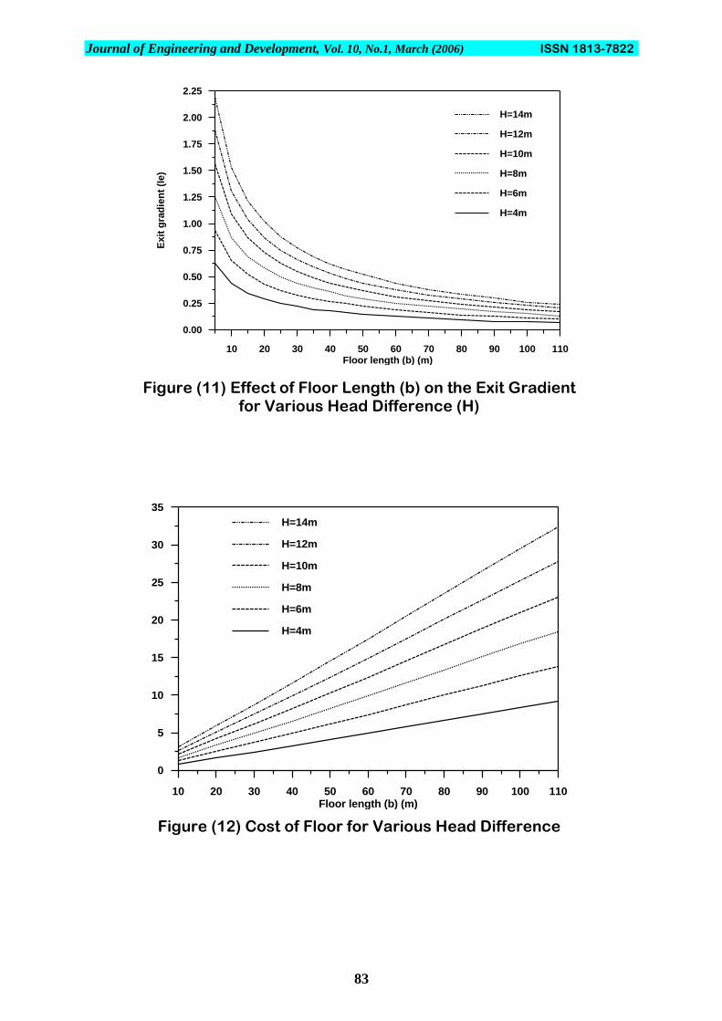
The relationship between the cost of floor and its length (b) for each head difference is

direct, i.e., cost increases with the increase of the floor length, as shown in Fig.(12).

Figure (13) shows the total costs (Z) for upstream blanket length (b1) and floor length

(b) with safe exit gradient. This figure could be used to find the necessary upstream blanket

length (b1) for any floor length (b). Moreover, the total cost is decreased with increased

upstream blanket length (b1), but it increases with increased floor length (b) for all the

considered values of head difference (H).


83

10 20 30 40 50 60 70 80 90 100 110Floor length (b) (m)

0.00

0.25

0.50

0.75

1.00

1.25

1.50

1.75

2.00

2.25

Ex

it g

rad

ien

t (I

e)

H=14m

H=12m

H=10m

H=8m

H=6m

H=4m

Figure (11) Effect of Floor Length (b) on the Exit Gradient for Various Head Difference (H)

10 20 30 40 50 60 70 80 90 100 110Floor length (b) (m)

0

5

10

15

20

25

30

35

H=14m

H=12m

H=10m

H=8m

H=6m

H=4m

Figure (12) Cost of Floor for Various Head Difference


84

0 10 20 30 40 50 60 70 80 90Length (m)

0

2

4

6

8

10

b1-curves b-curves Ie=0.25

H=4m

H=6m

H=8m

(a) For (H=4 , 6 , and 8 m)

0 10 20 30 40 50 60 70 80 90 100 110 120 130 140 150 160Length (m)

0

5

10

15

20

25

30

35

40

b1-curves b-curves

Ie=0.25

H=10m

H=12m

H=14m

(b) For (H=10 , 12 , and 14 m)

Figure (13) Total Cost for U/S Blanket Length(b1) and Floor Length(b),with Safe Exit Gradient


85

Figure (14) shows the total cost (Z) for both downstream cut-off and the floor, for the

considered head difference. The total cost decreases with the increase of the downstream cut-

off depth whereas it increases with the increase of floor length. The figure could be used to

find the necessary downstream cut-off depth (d2) for any floor length (b).

For each head difference value (H), an optimum design (minimum total cost) could be

found from the feasible solutions.

0 10 20 30 40 50 60 70 80 90 100 110Length (m)

0

5

10

15

20

25

30

d2-curves

b-curves

H=4m

H=6m

H=8m

(a) For (H= 4 , 6 , and 8 m)

0 20 40 60 80 100 120 140 160 180 200 220 240Length (m)

0

20

40

60

80

100

120

140

d2-curvesb-curves

H=10m

H=12m

H=14m

(b) For (H= 10 , 12 , and 14 m)

Figure (14) Total Cost for Both D/S Cut-Off (d2) and the Floor (b), with Safe Exit Gradient


86

Table (1) summarizes the final results of running the optimization model. The table

indicates that the filter trench gives a more economical cost than the upstream blanket,

upstream cut-off and downstream cut-off.

Table (1) Optimum Design of Control Devices

(Lagrange-Multiplier Method)

Dif

f .

Hea

d (

H)

(m)

Flo

or

Len

gth

(b

)

(m)

U/S

Bla

nk

et (

b1)

(m)

U/S

Cu

t-O

ff (

d1)

(m)

D/S

Cu

t-O

ff (

d2)

(m)

Total Cost (106 in I.D./m)

With

Filter Trench

Without

Filter Trench

4 3.0 8 3 5 1.0504 1.2503

6 8.5 10 3.5 6.5 1.7894 2.1973

8 15 13 4.5 7 2.7437 3.4261

10 20 15 6 8.5 3.3936 5.2810

12 32 18 9 9.5 4.2226 7.1978

14 40 22 10 11 5.6693 11.4581

7. Conclusions

The following conclusions have been abstracted:

1. The uplift pressure decreases with the increase in U/S length of the blanket; the same holds

true with the exit gradient. However, the uplift pressure and exit gradient increase when

using a D/S blanket.

2. The D/S cut-off is more effective than the U/S cut-off in terms of the reduction of the exit

gradient.

3. The pressure head U/S and D/S of the filter trench decreases as the width or depth of filter

increases; this remains true with the exit gradient. Also, the exit gradient decreases as the

filter trench is moved from U/S to D/S.

4. The uplift pressure and exit gradient would decrease with increasing the (width / depth)

ratio for the same sectional area of filter.

5. For a hydraulic structure with U/S blanket of various lengths, a blanket of (zero) length

gives the maximum floor cost for all applied head differences.

6. For a hydraulic structure with U/S cut-off of various depths, the total cost decreases with

increasing the depth of the U/S cut-off and decreasing the length of the floor. The

minimum total cost is attained when the maximum U/S cut-off depth is used. This remains

true regardless of using a D/S cut-off.

7. Using the U/S cut-off is more economical than using the D/S cut-off.

8. For a hydraulic structure with different control devices, the minimum total cost could be

achieved when a filter trench is used.


87

8. References

1. Terzaghi, K., and Peck, R. B., “Soil Mechanics Engineering Practice”, John Wily

and Sons, U.S.A, 1967.

2. Conner, J. J., and Brebbia, C. A., “Finite Element Technique for Fluids Flow”,

Newnes-Butter Worths, 1976.

3. Cechi, M. M., and Mancino, O. G., “The Generalized Problem of Confined

Seepage”, International Journal for Numerical Method in Engineering, Vol.(12),

1978, pp.479-486.

4. Zienkiewicz, O. C., “The Finite Element in Engineering Sciences”, McGraw-Hill

Co., 1982.

5. Nassir, H. A. A., “Seepage Analysis Below Hydraulic Structures Applying Finite

Element Method”, M.Sc. Thesis, Department of Civil Engineering, University of

Basrah, 1984.

6. Hatab, A. M. A., “Seepage Analysis Below Hydraulic Structures with Subsurface

Drains”, M.Sc. Thesis, Department of Civil Engineering, University of Basrah,

1987.

7. Ijam, A. Z., and Hatab, A. M. A., “Stability of Hydraulic Structures with Vertical

Drains”, Journal of Engineering and Technology, Baghdad, Vol.(10), No.1, 1993.

8. Ijam, A. Z., and Nassir, H. A. A., “Seepage Below Hydraulic Structures with Two

Cut-Offs”, Journal of Engineering, Baghdad, Vol.(5), No.3, 1988.

9. Khsaf, S. I., “Numerical Analysis of Seepage Problems with Flow Control Devices

underneath Hydraulic Structures”, Ph.D. Thesis, Department of Building and

Construction Engineering, University of Technology, 1998.

10. Gill, M. A., “Theory of Blanket Design for Dams on Pervious Foundation”,

Journal of Hydraulic Research, No.4, 1980, pp.299-311.

11. Bennett, P. T., “The Effect of Blankets on Seepage Through Pervious

Foundations”, Transactions, ASCE, Vol.111, 1946, pp.215-228.

12. Hamed, W., “Optimum Design of Barrage Floors”, M.Sc. Thesis, Department of

Civil Engineering, University of Baghdad, 1996.

13. Harr, M. E., “Groundwater and Seepage”, McGraw-Hill Book Company, 1962.

14. Segrlind, L. J., “Applied Finite Element Analysis”, John Wiley and Sons, Inc.,

New York, 1976.

15. Burnett, D. S., “Finite Element Analysis form Concepts to Applications”,

Addison-Wesley Publishing Company, London, 1987.

16. Irons, B. M., “A Frontal Solution Program for Finite Element Analysis”,

International Journal for Numerical Method in Engineering, Vol.(2), 1970, pp.5-32.

Documents

Optimum Design of Control Devices for Safe Seepage under Hydraulic