Embed Size (px)
Citation preview
Optimum Transmission Policies for BatteryLimited Energy Harvesting Nodes
Kaya Tutuncuoglu Aylin YenerWireless Communications and Networking Laboratory (WCAN)
Electrical Engineering DepartmentThe Pennsylvania State University, University Park, PA 16802
[email protected] [email protected]
Abstract
Wireless networks with energy harvesting battery equipped nodes are quickly emerging as a viable
option for future wireless networks with extended lifetime. Equally important to their counterpart in the
design of energy harvesting radios are the design principles that this new networking paradigm calls
for. In particular, unlike wireless networks considered to date, the energy replenishment process and
the storage constraints of the rechargeable batteries need to be taken into account in designing efficient
transmission strategies. In this work, such transmission policies for rechargeable nodes are considered,
and optimum solutions for two related problems are identified. Specifically, the transmission policy that
maximizes the short term throughput, i.e., the amount of data transmitted in a finite time horizon is
found. In addition, the relation of this optimization problem to another, namely, the minimization of the
transmission completion time for a given amount of data is demonstrated, which leads to the solution
of the latter as well. The optimum transmission policies are identified under the constraints on energy
causality, i.e., energy replenishment process, as well as the energy storage, i.e., battery capacity. For
battery replenishment, a model with discrete packets of energy arrivals is considered. The necessary
conditions that the throughput-optimal allocation satisfies are derived, and then the algorithm that finds
the optimal transmission policy with respect to the short-term throughput and the minimum transmission
completion time is given. Numerical results are presented to confirm the analytical findings.
This work was supported by NSF Grant CNS 0964364. The conference paper [1], scheduled to appear at ICC 2011, containstechnical material in part from the short term throughput optimization problem considered in this submission.
arX
iv:1
010.
6280
v2 [
cs.I
T]
8 J
un 2
011
1
I. INTRODUCTION
With the wide deployment of battery powered wireless devices, prolonging the lifetime of
wireless networks is becoming ever more critical [2]. Systems powered with batteries suffer
from a limited lifetime, whereas networks consisting of energy harvesting or rechargeable nodes
can survive perpetually [3]. The performance that such systems can deliver is tied closely to
efficient utilization of energy that is currently available, as well as that is to be harvested. Towards
understanding fundamental performance limits with energy harvesting, in this work, we iden-
tify optimal transmission policies for maximizing throughput and minimizing the transmission
completion time of a wireless node with a replenishing energy source and a finite battery.
There has been a significant amount of previous work in energy efficient communications and
networking of nodes with non-rechargeable batteries, from the perspective of various protocol
layers, or cross-layer approaches, e.g. [4]–[12]. References relevant to this paper include [4], [5].
Energy efficient deadline-constrained communications is considered in [4] resulting in a packet
scheduling algorithm that achieves minimum energy. In [5], an insightful approach to energy-
efficient rate control is developed and the problem with individual deadline or buffer constrained
systems with data arrivals is solved.
There has also been some recent interest in wireless networks with energy harvesting nodes.
A queue stabilizing transmission policy is developed in [13] for a recharging battery powered
transmitter. This is a modified adaptive backpressure policy that is shown to be asymptotically
optimal for sufficiently large battery capacity. Reference [14] calculates energy management
policies that are throughput optimal or mean delay optimal, and shows that a greedy policy
is optimal for both problems in low SNR regime. A discrete-time battery model is introduced
in [15] for the problem of energy aware routing in wireless networks powered with renewable
energy. Reference [16] assumes a Markov model for battery state, and proposes a threshold
algorithm to best utilize available energy to packets with different rewards. In [17], policies
based on the energy-error probability tradeoff are developed to maximize successful transmission
probability while minimizing probability of running out of energy in an energy harvesting body
sensor network. For a solar powered wireless network, [18] lays out sleep/wake-up strategies

2
for various factors and determines optimal parameters of the solar energy harvest based strategy
using a bargaining game model. The most relevant reference work to the present paper is [19],
[20], where the authors have considered an energy harvesting node, and found transmission
policies that minimize the transmission completion time of a given amount of data. This work
assumes an infinite capacity battery for the energy harvesting transmitter.
In this paper, we consider the problem of maximizing the short-term throughput of an energy
harvesting node, in other words, maximizing the data transferred under a deadline constraint.
Unlike previous work [19], we employ the realistic constraint that an energy harvesting battery
must have finite energy storage capacity. We seek to find the optimum transmission policy under
this energy storage constraint as well as the energy causality constraint. That is to say that, due
to the finite battery at the transmitter, any received energy that overflows its capacity is lost, and,
that energy can not be expended prior to being harvested. Like previous work [19], we consider
known energy arrivals, in order to find a bench mark solution for any transmission policy that
considers communication under a deadline. We also show that the problem solved in this paper
is closely related to the problem of transmission completion time minimization considered in
[19]. Specifically, we show that the solution to the former is identical to that of the latter for
the same parameters, providing a solution to the latter under battery storage constraints as well.
The algorithm that finds the optimum power allocation to solve the former is developed. Then,
using the relation between the two problems, a similar algorithm that finds the optimum power
allocation to minimize the transmission completion time is presented.
The remainder of the paper is organized as follows. The system model and the problem
definition is presented in Section II. Section III solves the short-term throughput maximization
problem and presents the optimal policy. Section IV addresses the completion time optimization
problem. Numerical results are presented in Section V followed by concluding remarks in
Section VI.
3
II. SYSTEM MODEL AND PROBLEM DEFINITION
We assume a single link continuous time system where a node transmits continuously and its
rate can be varied at will via power control. Specifically, the transmitter can choose to transmit
with power P (t) at any instant t, achieving a corresponding rate r(p(t)) where r(.) is a non-
negative, increasing, strictly concave function that we will refer to as the power-rate function.
Using a power-rate function of this form is fairly common [5], [20], and is clearly valid for
the additive white Gaussian noise (AWGN) channel. Factors such as processing power, battery
leakage or base energy consumption are not explicitly taken into account in this model, however,
can be integrated in the power-rate function without violating its above stated properties. For
example, a base energy consumption of power Pb could be modeled as a shift in the power rate
function horizontally by Pb, or a processing power linear in transmission rate could be added to
r(.) to yield a new power-rate function satisfying the same properties.
We consider an energy harvesting system with a finite-capacity battery. That is to say that
the battery can store up to Emax. This storage capacity is considered to be constant throughout
the transmission horizon, i.e., battery wear or fatigue is assumed to be much slower than the
time scale of the problem. The property of keeping the battery energy below its capacity and
non-negative, i.e. within [0, Emax], will be referred to as energy-feasibility in the sequel.
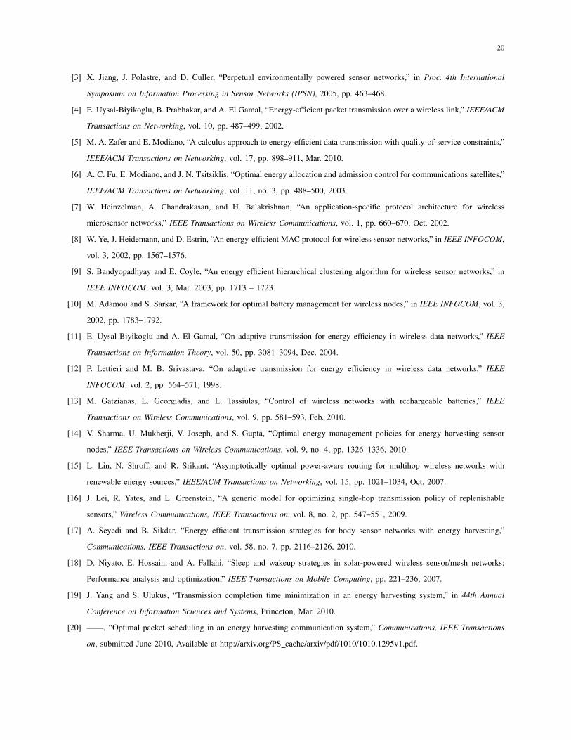
We will consider the offline optimization problem. Hence the energy replenishment process
is modeled as a discrete process with energy harvests of size En arriving at time instances sn,
as shown in Figure 1, where En and sn take positive real values and are available non-causally
to the transmitter at the beginning of transmission. The first energy arrival E0 is conventionally
at time s0 = 0, representing the initial energy in the battery. Due to the limited battery, if the
harvested energy En is larger than the available space in the battery at time sn, the battery is
charged to maximum capacity and the remainder of the energy packet is discarded. Note that an
instantaneous energy consumption requires infinite instantaneous power, which is not allowed
by system definition. Thus, all harvested energy must first be stored before consumption. Based
on this observation, it is safe to assume that En ≤ Emax, as no more than an Emax amount of
a harvest can be utilized by the transmitter. Therefore, a truncation at Emax for En values will

4
be assumed in the sequel.
An example to justify this model could be a solar powered surveillance network. A continuous
operation would be necessary for surveillance purposes, and the nodes would realistically be
operating on finite batteries. Once the nodes are deployed, the solar energy harvesting process
would be predictable enough to have good estimates of En and sn, yet significantly varying
throughout the day.
In this model, the amount of energy available at any time instant is constrained, either because
a sufficient amount may not yet be harvested or cannot be stored in the battery. As such, we
have an energy-feasibility constraint on the transmission policy. Specifically, a energy-feasible
power allocation p(t) is a bounded non-negative function for the transmission power that ensures
the battery state stays within [0, Emax]. We express the set of energy-feasible power allocation
functions as
P = { p(t) | 0 ≤n−1∑k=0
Ek −∫ t′
0
p(t)dt ≤ Emax, sn−1 ≤ t′ ≤ sn } (1)
which is a convex set of functions, i.e., any convex combination of two energy feasible allocations
is also energy feasible. Note that allocation functions which lead to a battery overflow are
physically possible, but are discarded from the energy-feasible set due to being strictly suboptimal
as shown in subsequent sections of this paper.
Our goal is to find the optimum power allocation for maximizing the total data transferred
from an energy harvesting node under a deadline constraint. The only constraint induced by the
model on the power allocation is the feasibility set P. The objective is to maximize the total
number of bits departed in the time interval [0, T ] over p(t). Under a rate function r(p(t)) and
a time deadline T the problem can be expressed as:
P1 : maxp(t)
∫ T
0
r(p(t))dt, s.t. p(t) ∈ P (2)
Next, we shall solve this problem.
5
III. SHORT-TERM THROUGHPUT MAXIMIZATION
This section considers the throughput maximization problem for an energy harvesting node
with infinite backlog and finite time. First, the necessary properties of the optimal policy are
established. Then, an algorithm is presented to generate the policy that satisfies all the necessary
conditions and the optimality of this policy is shown.
A. Optimality conditions
The following lemmas provide the necessary conditions for a power allocation policy to
be optimal. These conditions provide valuable insight into the development of the algorithm
proposed in Section III-B and the proof of its optimality.
Lemma 1: Given the total amount of energy consumed in any time interval [t1, t2], a constant-
power transmission is throughput optimal, i.e., among all transmission policies consuming energy
E, the constant-power transmission p(t) = Et2−t1 departs the largest number of bits.
Proof: The proof is by contradiction. Assume that p(t) is non-uniform in (t1, t2) , i.e.,
for τ1, τ2 ∈ (t1, t2), τ1 6= τ2, we have p(τ1) 6= p(τ2). Without loss of generality, assume that
p(τ1) < p(τ2). Keeping p(t) unchanged at every other time instance, we define an alternative
policy p′(t) as
p′(t) =
p(t) + δ t ∈ [τ1, τ1 + ε]
p(t)− δ t ∈ [τ2, τ2 + ε]
p(t) otherwise.
(3)
where δ > 0 is an infinitesimal power displacement among two intervals of arbitrarily small
duration ε > 0. Clearly, the energy consumed by p(t) and p′(t) are equal. However calculating
the information sent in [t1, t2] yields
B =
∫ t2
t1
r(p(t)) dt
=
∫ τ1
t1
r(p(t)) dt+
∫ τ2
τ1+ε
r(p(t)) dt+
∫ t2
τ2+ε
r(p(t)) dt+ [r(p(τ1)) + r(p(τ2))].ε

6
<
∫ τ1
t1
r(p(t)) dt+
∫ τ2
τ1+ε
r(p(t)) dt+
∫ t2
τ2+ε
r(p(t)) dt+ (r(p(τ1) + δ) + r(p(τ2)− δ)).ε
(4)
=
∫ t2
t1
r(p′(t)) dt = B′
where the inequality in (4) follows from the definition of strict concavity for r(p). This shows
that we can strictly improve the throughput by equalizing the two power values, and by extension
uniformizing the power allocation.
Corollary 1: The optimal power allocation policy dictates the transmission power, and thus
the rate, remains constant between energy arrivals. Consequently the power level can change
only when a new energy packet arrives. This follows from Lemma 1, by considering the interval
[sn, sn+1] and introducing the feasibility definition in (1) to the optimization. However, given a
total consumed energy in [sn, sn+1], feasibility in the sense defined in (1) does not depend on
the structure of p(t) in this interval. Thus the constant power policy is feasible, and therefore
optimal for any given energy consumed.
Lemma 2: Any power allocation policy yielding a battery overflow is strictly suboptimal.
Proof: It is clear that the battery cannot possibly overflow without an energy arrival. Therefore,
we start by assuming that the battery overflows at the energy arrival instant si. Let the power
allocation allowing this overflow be p(t). Ei is less than or equal to Emax by system model
and causes an overflow, thus battery state at s−i is strictly positive. This implies that p(t) can
be increased by an infinitesimal amount δ in (si − ε, si) without violating energy-feasibility,
which strictly increases the throughput. Since the excess energy required, δ.ε, is recovered by
the overflow at si, the remaining transmission schedule remains unchanged. Therefore, a power
allocation that yields a battery overflow can not be optimal.
Lemma 3: In the optimal power allocation, the transmission power does not change unless
the battery is either full or completely depleted.

7
Proof: Assume that at arbitrary time t transmission power changes, so that p(t−) 6= p(t+).
Consider the interval [t− τ, t+ τ ], where the policy depletes a total energy of τ.(p(t−) + p(t+)).
Unless the battery is full or depleted at t, the energy feasibility constraints will be inactive in
this interval. Let p∗(t) = p(t−)+p(t+)2
be the constant power transmission policy in [t − τ, t + τ ]
that expends the same total energy, which is also feasible for τ sufficiently small, due to energy
feasibility constraints being locally inactive around t. Then, p(t) can be replaced with p∗(t)
without altering the rest of the problem, and due to Lemma 1, departs strictly more bits. Thus,
p(t) must be stay constant unless an energy feasibility constraint is active, i.e. the battery is
either full or depleted.
Note that in the proof above, p∗(t) might still be feasible when battery is full or depleted,
specifically if it shifts the policy away from the active constraint. This observation forms the
grounds of the next lemma:
Lemma 4: For optimal power allocation, the change in power level pn at an energy arrival
instant sn has to be nonnegative (nonpositive) if the battery is depleted (full) at that time instant.
Proof: The proof is by contradiction. Consider the notation in the proof of Lemma 3. Battery
being depleted at time t implies that the first inequality in (1) is active. However, if p(t−) > p(t+)
holds, i.e. if transmission power is decreasing, then p∗(t) < p(t). Hence replacing p(t) with p∗(t)
on [t− τ, t+ τ ] increases the RHS of the active inequality, which is feasible. This shows that if
the battery is depleted at t, a decreasing power policy at t can not be optimal. Similarly, battery
being full at time t implies that the second inequality in (1) is active. This time, an increasing
power policy, p(t−) < p(t+), implies p∗(t) > p(t); which renders replacing p(t) with p∗(t) on
[t− τ, t+ τ ] feasible. This proves the second statement of the lemma.
Corollary 2: Lemmas 3 and 4 together imply that for optimal power allocation, transmission
power decreases only at energy arrival instants when the battery is full and increases only at
energy arrival instants when the battery is depleted.
Lemma 5: The optimal power allocation expends all harvested energy by the end of the
transmission.
8
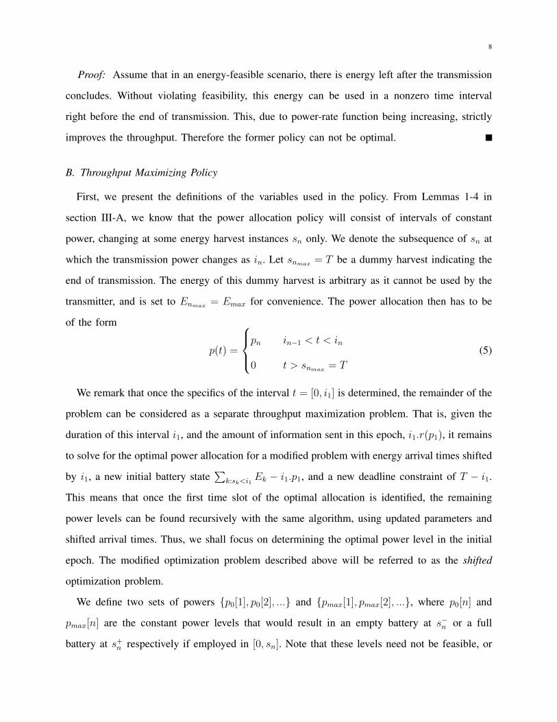
Proof: Assume that in an energy-feasible scenario, there is energy left after the transmission
concludes. Without violating feasibility, this energy can be used in a nonzero time interval
right before the end of transmission. This, due to power-rate function being increasing, strictly
improves the throughput. Therefore the former policy can not be optimal.
B. Throughput Maximizing Policy
First, we present the definitions of the variables used in the policy. From Lemmas 1-4 in
section III-A, we know that the power allocation policy will consist of intervals of constant
power, changing at some energy harvest instances sn only. We denote the subsequence of sn at
which the transmission power changes as in. Let snmax = T be a dummy harvest indicating the
end of transmission. The energy of this dummy harvest is arbitrary as it cannot be used by the
transmitter, and is set to Enmax = Emax for convenience. The power allocation then has to be
of the form
p(t) =
pn in−1 < t < in
0 t > snmax = T
(5)
We remark that once the specifics of the interval t = [0, i1] is determined, the remainder of the
problem can be considered as a separate throughput maximization problem. That is, given the
duration of this interval i1, and the amount of information sent in this epoch, i1.r(p1), it remains
to solve for the optimal power allocation for a modified problem with energy arrival times shifted
by i1, a new initial battery state∑
k:sk<i1Ek − i1.p1, and a new deadline constraint of T − i1.
This means that once the first time slot of the optimal allocation is identified, the remaining
power levels can be found recursively with the same algorithm, using updated parameters and
shifted arrival times. Thus, we shall focus on determining the optimal power level in the initial
epoch. The modified optimization problem described above will be referred to as the shifted
optimization problem.
We define two sets of powers {p0[1], p0[2], ...} and {pmax[1], pmax[2], ...}, where p0[n] and
pmax[n] are the constant power levels that would result in an empty battery at s−n or a full
battery at s+n respectively if employed in [0, sn]. Note that these levels need not be feasible, or
9
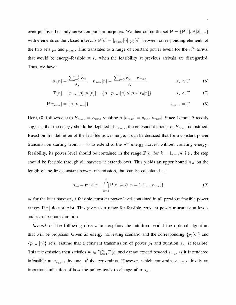
even positive, but only serve comparison purposes. We then define the set P = {P[1],P[2], ...}
with elements as the closed intervals P[n] = [pmax[n], p0[n]] between corresponding elements of
the two sets p0 and pmax. This translates to a range of constant power levels for the nth arrival
that would be energy-feasible at sn when the feasibility at previous arrivals are disregarded.
Thus, we have:
p0[n] =
∑n−1k=0 Eksn
, pmax[n] =
∑nk=0Ek − Emax
snsn < T (6)
P[n] = [pmax[n], p0[n]] = {p | pmax[n] ≤ p ≤ p0[n]} sn < T (7)
P[nmax] = {p0[nmax]} snmax = T (8)
Here, (8) follows due to Enmax = Emax yielding p0[nmax] = pmax[nmax]. Since Lemma 5 readily
suggests that the energy should be depleted at snmax , the convenient choice of Enmax is justified.
Based on this definition of the feasible power range, it can be deduced that for a constant power
transmission starting from t = 0 to extend to the nth energy harvest without violating energy-
feasibility, its power level should be contained in the range P[k] for k = 1, ..., n, i.e., the step
should be feasible through all harvests it extends over. This yields an upper bound nub on the
length of the first constant power transmission, that can be calculated as
nub = max{n |n⋂k=1
P[k] 6= ∅, n = 1, 2, .., nmax} (9)
as for the later harvests, a feasible constant power level contained in all previous feasible power
ranges P[n] do not exist. This gives us a range for feasible constant power transmission levels
and its maximum duration.
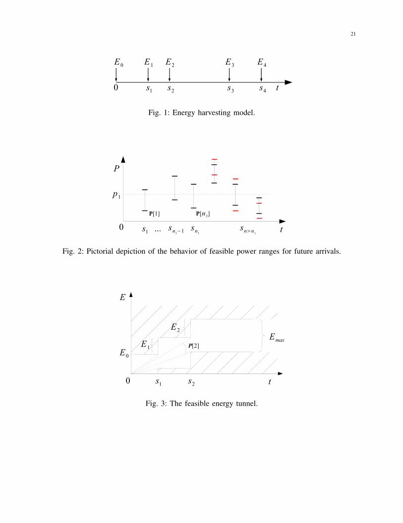
Remark 1: The following observation explains the intuition behind the optimal algorithm
that will be proposed. Given an energy harvesting scenario and the corresponding {p0[n]} and
{pmax[n]} sets, assume that a constant transmission of power p1 and duration sn1 is feasible.
This transmission then satisfies p1 ∈⋂n1
k=1 P[k] and cannot extend beyond snub, as it is rendered
infeasible at snub+1 by one of the constraints. However, which constraint causes this is an
important indication of how the policy tends to change after sn1 .
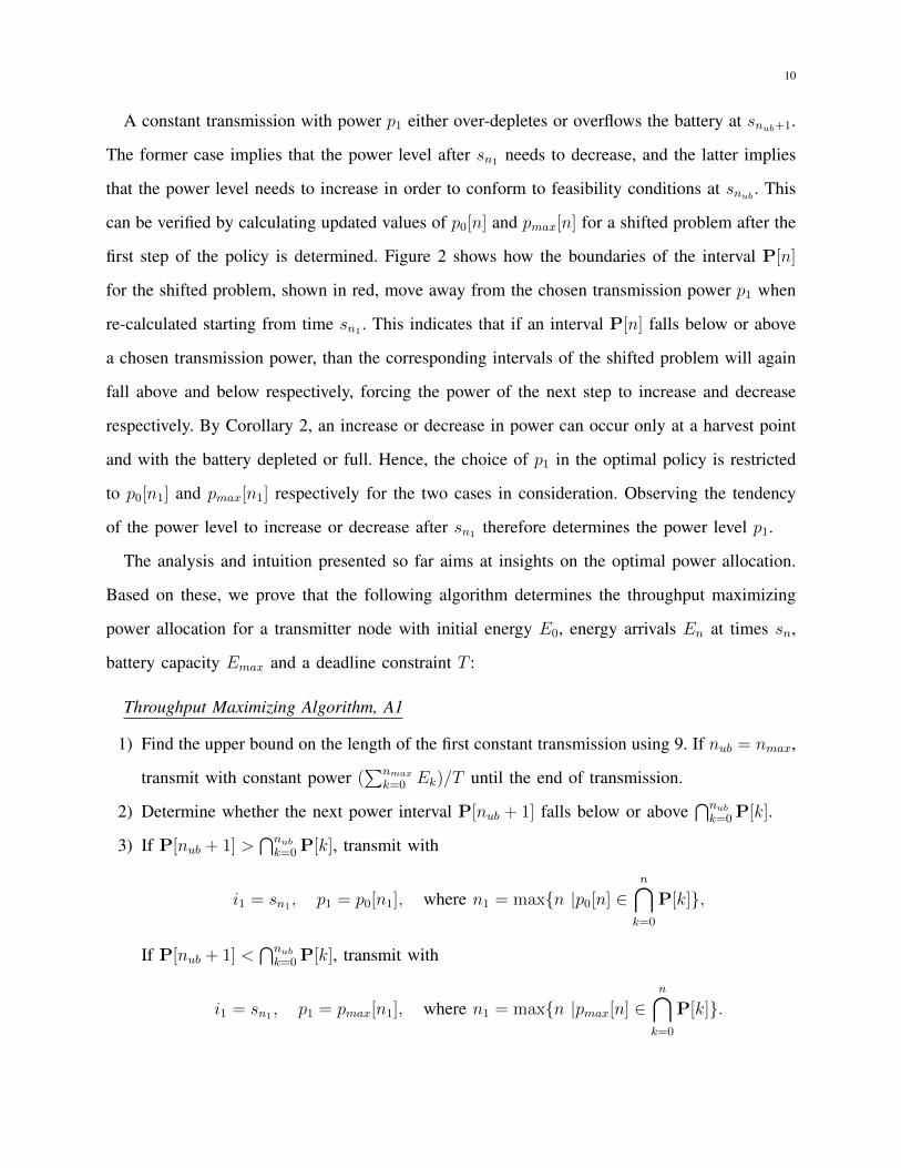
10
A constant transmission with power p1 either over-depletes or overflows the battery at snub+1.
The former case implies that the power level after sn1 needs to decrease, and the latter implies
that the power level needs to increase in order to conform to feasibility conditions at snub. This
can be verified by calculating updated values of p0[n] and pmax[n] for a shifted problem after the
first step of the policy is determined. Figure 2 shows how the boundaries of the interval P[n]
for the shifted problem, shown in red, move away from the chosen transmission power p1 when
re-calculated starting from time sn1 . This indicates that if an interval P[n] falls below or above
a chosen transmission power, than the corresponding intervals of the shifted problem will again
fall above and below respectively, forcing the power of the next step to increase and decrease
respectively. By Corollary 2, an increase or decrease in power can occur only at a harvest point
and with the battery depleted or full. Hence, the choice of p1 in the optimal policy is restricted
to p0[n1] and pmax[n1] respectively for the two cases in consideration. Observing the tendency
of the power level to increase or decrease after sn1 therefore determines the power level p1.
The analysis and intuition presented so far aims at insights on the optimal power allocation.
Based on these, we prove that the following algorithm determines the throughput maximizing
power allocation for a transmitter node with initial energy E0, energy arrivals En at times sn,
battery capacity Emax and a deadline constraint T :
Throughput Maximizing Algorithm, A1
1) Find the upper bound on the length of the first constant transmission using 9. If nub = nmax,
transmit with constant power (∑nmax
k=0 Ek)/T until the end of transmission.
2) Determine whether the next power interval P[nub + 1] falls below or above⋂nub
k=0P[k].
3) If P[nub + 1] >⋂nub
k=0P[k], transmit with
i1 = sn1 , p1 = p0[n1], where n1 = max{n |p0[n] ∈n⋂k=0
P[k]},
If P[nub + 1] <⋂nub
k=0P[k], transmit with
i1 = sn1 , p1 = pmax[n1], where n1 = max{n |pmax[n] ∈n⋂k=0
P[k]}.
11
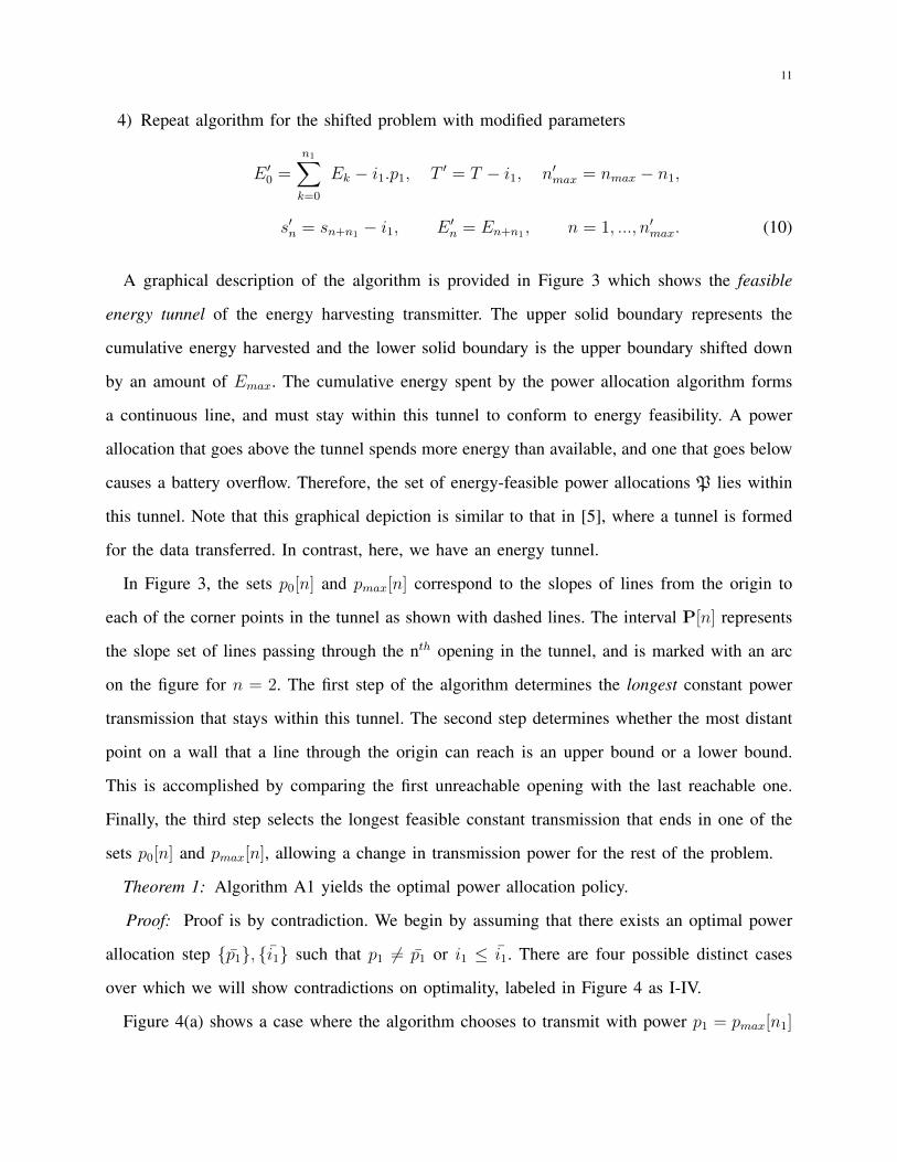
4) Repeat algorithm for the shifted problem with modified parameters
E ′0 =
n1∑k=0
Ek − i1.p1, T ′ = T − i1, n′max = nmax − n1,
s′n = sn+n1 − i1, E ′n = En+n1 , n = 1, ..., n′max. (10)
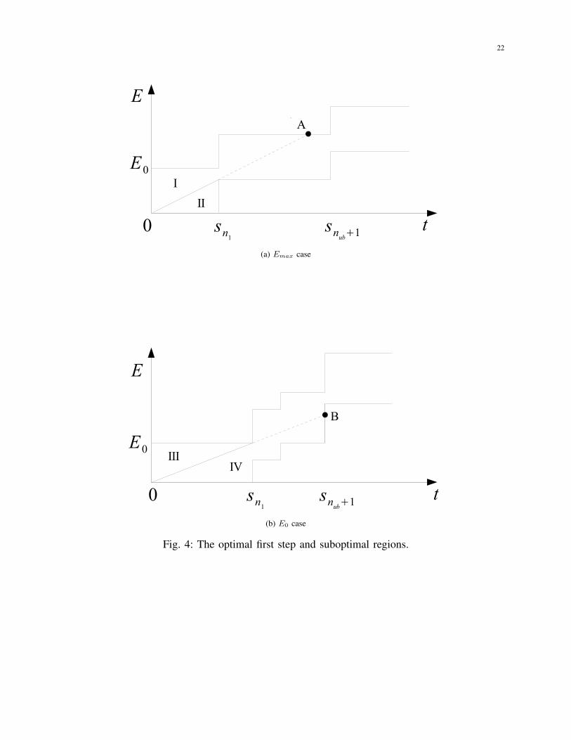
A graphical description of the algorithm is provided in Figure 3 which shows the feasible
energy tunnel of the energy harvesting transmitter. The upper solid boundary represents the
cumulative energy harvested and the lower solid boundary is the upper boundary shifted down
by an amount of Emax. The cumulative energy spent by the power allocation algorithm forms
a continuous line, and must stay within this tunnel to conform to energy feasibility. A power
allocation that goes above the tunnel spends more energy than available, and one that goes below
causes a battery overflow. Therefore, the set of energy-feasible power allocations P lies within
this tunnel. Note that this graphical depiction is similar to that in [5], where a tunnel is formed
for the data transferred. In contrast, here, we have an energy tunnel.
In Figure 3, the sets p0[n] and pmax[n] correspond to the slopes of lines from the origin to
each of the corner points in the tunnel as shown with dashed lines. The interval P[n] represents
the slope set of lines passing through the nth opening in the tunnel, and is marked with an arc
on the figure for n = 2. The first step of the algorithm determines the longest constant power
transmission that stays within this tunnel. The second step determines whether the most distant
point on a wall that a line through the origin can reach is an upper bound or a lower bound.
This is accomplished by comparing the first unreachable opening with the last reachable one.
Finally, the third step selects the longest feasible constant transmission that ends in one of the
sets p0[n] and pmax[n], allowing a change in transmission power for the rest of the problem.
Theorem 1: Algorithm A1 yields the optimal power allocation policy.
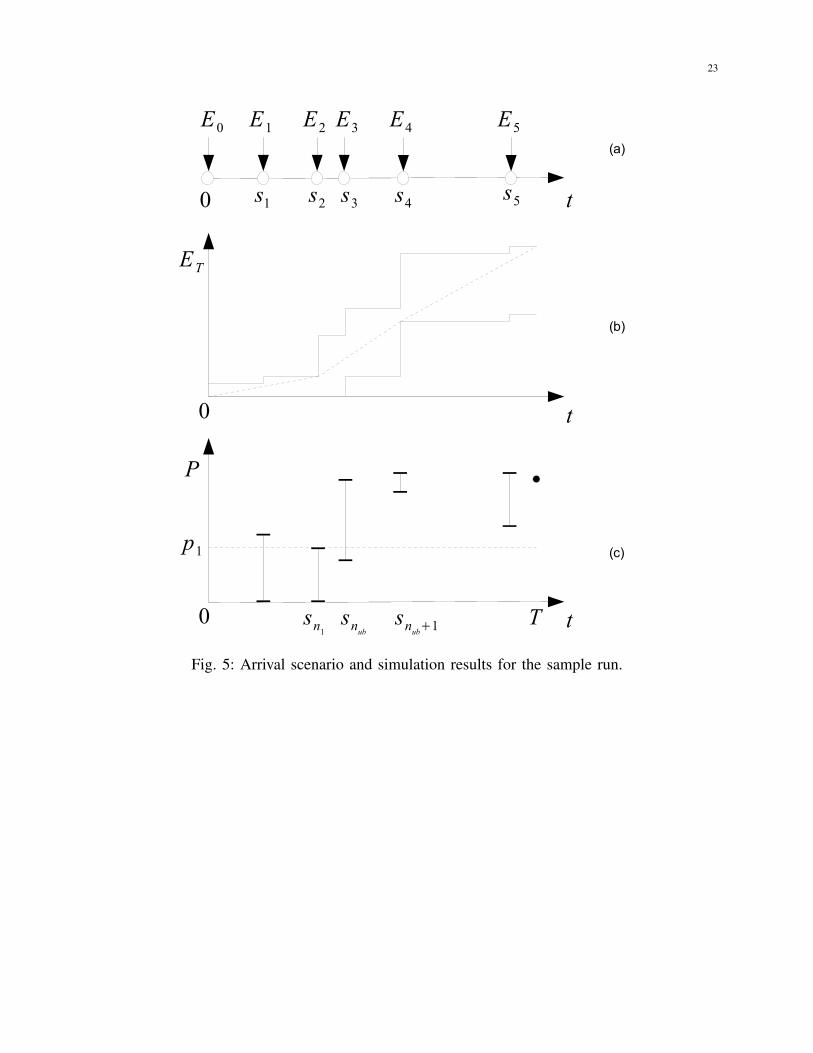
Proof: Proof is by contradiction. We begin by assuming that there exists an optimal power
allocation step {p1}, {i1} such that p1 6= p1 or i1 ≤ i1. There are four possible distinct cases
over which we will show contradictions on optimality, labeled in Figure 4 as I-IV.
Figure 4(a) shows a case where the algorithm chooses to transmit with power p1 = pmax[n1]
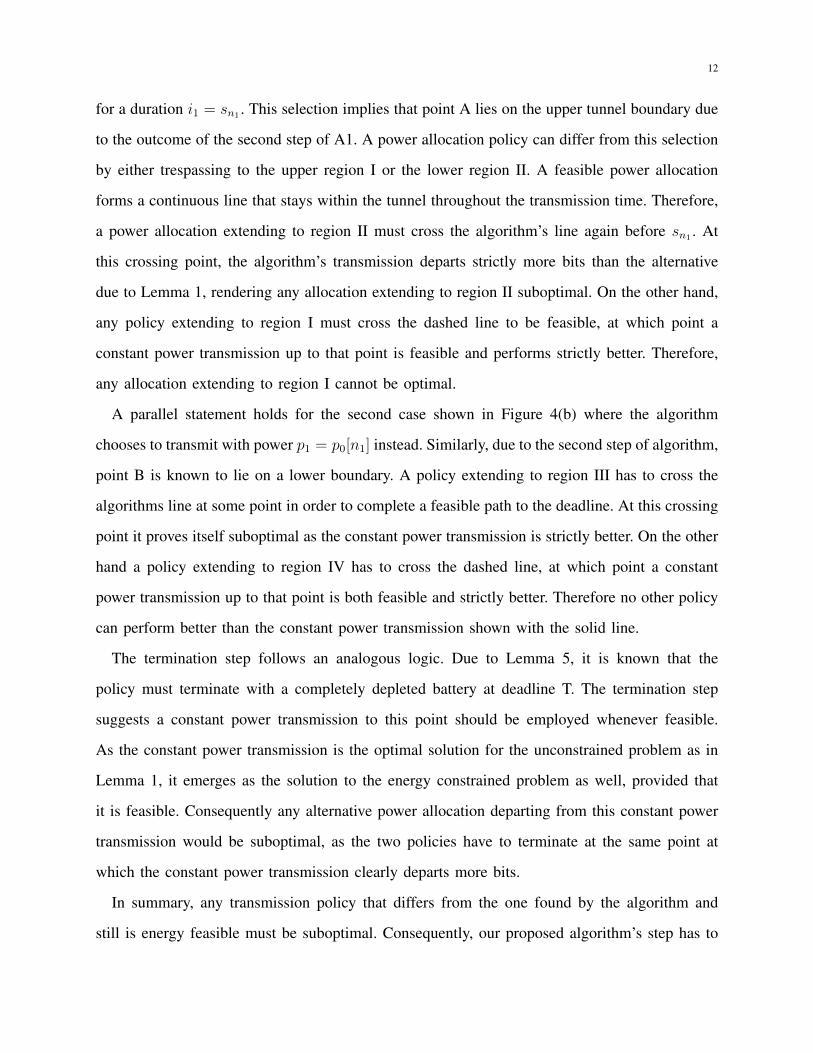
12
for a duration i1 = sn1 . This selection implies that point A lies on the upper tunnel boundary due
to the outcome of the second step of A1. A power allocation policy can differ from this selection
by either trespassing to the upper region I or the lower region II. A feasible power allocation
forms a continuous line that stays within the tunnel throughout the transmission time. Therefore,
a power allocation extending to region II must cross the algorithm’s line again before sn1 . At
this crossing point, the algorithm’s transmission departs strictly more bits than the alternative
due to Lemma 1, rendering any allocation extending to region II suboptimal. On the other hand,
any policy extending to region I must cross the dashed line to be feasible, at which point a
constant power transmission up to that point is feasible and performs strictly better. Therefore,
any allocation extending to region I cannot be optimal.
A parallel statement holds for the second case shown in Figure 4(b) where the algorithm
chooses to transmit with power p1 = p0[n1] instead. Similarly, due to the second step of algorithm,
point B is known to lie on a lower boundary. A policy extending to region III has to cross the
algorithms line at some point in order to complete a feasible path to the deadline. At this crossing
point it proves itself suboptimal as the constant power transmission is strictly better. On the other
hand a policy extending to region IV has to cross the dashed line, at which point a constant
power transmission up to that point is both feasible and strictly better. Therefore no other policy
can perform better than the constant power transmission shown with the solid line.
The termination step follows an analogous logic. Due to Lemma 5, it is known that the
policy must terminate with a completely depleted battery at deadline T. The termination step
suggests a constant power transmission to this point should be employed whenever feasible.
As the constant power transmission is the optimal solution for the unconstrained problem as in
Lemma 1, it emerges as the solution to the energy constrained problem as well, provided that
it is feasible. Consequently any alternative power allocation departing from this constant power
transmission would be suboptimal, as the two policies have to terminate at the same point at
which the constant power transmission clearly departs more bits.
In summary, any transmission policy that differs from the one found by the algorithm and
still is energy feasible must be suboptimal. Consequently, our proposed algorithm’s step has to
13
yield the optimal policy.
With the necessary conditions and algorithm A1 derived for the throughput maximization
problem, we move on to an alternative problem with similar results.
IV. TRANSMISSION COMPLETION TIME MINIMIZATION PROBLEM
A previous problem studied with an energy harvesting transmitter is the transmission comple-
tion time minimization problem, introduced in [20]. The transmission completion time minimiza-
tion problem focuses on determining an energy feasible power allocation p(t) ∈ P that, given
the total number of bits to send as B, finalizes the transmission in the shortest time possible.
This problem has total transmission time T as an objective function to be minimized, and a
throughput constraint as seen in the mathematical expression of the optimization problem:
P2 : min T, s.t. B −∫ T
0
r(p(t))dt ≤ 0, p(t) ∈ P (11)
In contrast to its throughput maximization counterpart we considered in Section III, the time
minimization problem appears to have a more complex form. Reference [20] solved this problem
by employing lemmas similar to the lemmas in Section III-A, without the battery constraints. To
address the model with finite battery capacity, an extension of the algorithm in [20] is possible.
However, we will choose another direction that is simpler.
Specifically, we note that although the throughput maximization problem differs significantly
in structure from the transmission completion time minimization problem, their solutions are
closely related. Theorem 2 states this relationship.
Theorem 2: For a given energy harvesting scenario, the two optimization problems yield
identical power allocation policies for matching time and bit constraints. In other words, if the
maximum-throughput policy for time interval [0, T ] departs a total of B bits, then the minimum-
time policy for B bits completes the transmission at time T , and vice versa.
Proof: First the Lagrangian dual problem of the time minimization problem in (11) is
formulated in (12). The variables T and p(t) of the nested minimization problem are by definition
independent. Keeping in mind that the solution to the dual problem satisfies u ≥ 0, the inner
14
problem can be separated as in (13). It can now be readily observed that the optimal power
allocation function p∗(t) arises from the solution of the maximization problem marked with P1
for the optimal completion time T ∗. Observe that P1 is identical to the throughput maximization
problem (2). Therefore the solution of the completion time minimization problem is identical to
the solution of the throughput maximization problem where the time constraint is the minimum
transmission completion time T ∗.
maxu≥0
(min
p(t)∈P,∀T(T + u(B −
∫ T
0
r(p(t) )dt) ))
(12)
maxu≥0
(min∀T
(T + u.B − u. maxp(t)∈P
∫ T
0
r(p(t))dt︸ ︷︷ ︸P1
))
(13)
Remark 2: An alternative proof is by making use of the monotonicity of the two problems
in time and bits. The minimum-time problem yields a strictly larger completion time for more
bits, while the maximum-throughput problem departs strictly more bits for a later deadline due
to the strict concavity of the power-rate function. Assume that the maximum-throughput policy
for interval [0, T ] departs a total of B bits but the minimum-time policy for B bits at time 0
completes the transmission at time T ′ 6= T . Consider the two cases T ′ > T and T ′ < T . The
contradiction in the first case T ′ > T is trivial as the maximum-throughput policy departs the
same number of bits in a shorter time; and thus the minimum-time policy cannot be optimal. In
the second case, minimum-time policy achieves the same throughput in a shorter time T ′ < T
indicating that there exists a shorter policy with the same throughput. Therefore strictly more than
B bits can be sent in the larger time interval [0, T ] and thus the suggested maximum-throughput
policy cannot be optimal.
Theorem 2 states that the solution to the former and latter problems are in fact identical.
Therefore Lemmas 1-5 that characterize the optimal power allocation also apply to the completion
time minimization problem. We make use of this relationship to develop a modified algorithm
that yields a throughput maximizing power allocation policy while departing exactly the desired
number of bits, thus solving the completion time minimization problem.
15
Remark 3: The two algorithms, i.e. the one that yields the throughput maximizing allocation
and the one that yields the completion time minimizing allocation, shall only differ in the
termination condition. Throughout the time interval in which a constant power transmission
until the end is not feasible, whether the end is defined by a deadline or end of a packet, the
power allocation shall be identical. Consequently, the two algorithms work identically until the
termination step is reached.
The throughput maximization policy terminates at a certain time in contrast to the completion
time minimization policy ending when a certain number of bits have been transmitted. Therefore
the definition of the feasible transmission interval P[n] in (6)-(8) needs to be modified as
p0[n] =
∑n−1k=0 Eksn
, pmax[n] =
∑nk=0Ek − Emax
sn, 0, p0[n].sn < B (14)
P[n] = {p|pmax[n] ≤ p ≤ p0[n]}, p0[n].sn < B (15)
P[nmax] = p0[nmax], p0[n].snmax = B (16)
where (16) suggests creating a virtual arrival point at snmax that corresponds to the point for
which a constant power transmission with the total energy harvested, ignoring energy constraints,
transmits all bits. This is the adapted version of the virtual arrival point approach in (8), and
can be interpreted as a candidate point for end of transmission that is selected if found feasible.
The point snmax lies between the two arrivals for which p0[ni].sni< B < p0[ni+1].sni+1
holds,
and can be found by solving the equation
B = snmax .r(
∑ni
k=0Eksni
), sni< snmax (17)
With the updated parameters we now provide the modified algorithm that yields the minimum
transmission completion time, and prove that the algorithm yields the optimal solution.
Transmission Completion Time Minimization Algorithm, A2
1) Find the upper bound on the length of the first constant transmission using 9. If nub = nmax
transmit with constant power (∑nmax
k=0 Ek)/snmax until end of transmission.
2) Determine whether the next power interval P[nub + 1] falls below or above⋂nub
k=0 P[k].
16
3) If P[nub + 1] >⋂nub
k=0P[k], transmit with
i1 = sn1 , p1 = p0[n1], where n1 = max{n |p0[n] ∈n⋂k=0
P[k]},
If P[nub + 1] <⋂nub
k=0P[k], transmit with
i1 = sn1 , p1 = pmax[n1], where n1 = max{n |pmax[n] ∈n⋂k=0
P[k]}.
4) Repeat algorithm for the shifted problem with modified parameters
E ′0 =
n1∑k=0
Ek − i1.p1, B′ = B − r(p1).sn1 , n′max = nmax − i1,
s′n = sn+n1 − i1, E ′n = En+n1 , n = 1, ..., n′max. (18)
Theorem 3: Algorithm A2 gives the optimal power allocation scheme for the transmission
completion time minimization problem.
Proof: We shall make use of the relation between the two problems to simplify this proof. If
the suggested power allocation with completion time T ∗ is identical to the throughput maximizing
allocation with a time constraint T ∗, we can state that no other allocation with time constraint
less than T ∗ can depart B bits, and therefore the allocation is optimal in time minimization.
This algorithm appears to differ from the throughput maximizing algorithm presented in
Section III at only two points: (14)-(16) and (18). However, (18) only affects the termination
condition through nmax in (16). Consequently the two allocations found using the two algorithms
are identical until either one reaches a termination step. The termination step of the time
minimization algorithm is reached when there exists a feasible constant power transmission step
that departs all the remaining bits by T ∗. The presence of this step implies that the matching
throughput maximization problem with deadline T ∗ would at the same time have the same
feasible constant power transmission opportunity and terminate. Conversely if there does not
exist a feasible last step departing all remaining bits, then T ∗ is unreachable by a constant power
transmission and the throughput maximization problem also fails to terminate. Thus we can state
17
that the matching algorithms terminating at the same time T ∗ would reach the termination step
at the same time.
The termination step on the other hand suggests a constant power transmission until the end
of transmission at T ∗. As the previous power policies for the two algorithms are identical, the
energies left for the last step are equal. Therefore for any termination step decided by the time
minimizing algorithm ending at T ∗, the throughput maximizing policy with the deadline T ∗
is forced to take the same step mainly because a constant power transmission is feasible with
the available energy. As a result, this algorithm yields a power allocation that is identical to a
maximum throughput solution, and is therefore optimal by Theorem 2.
V. SIMULATION RESULTS
In this section, we present simulation results to demonstrate the behavior and the performance
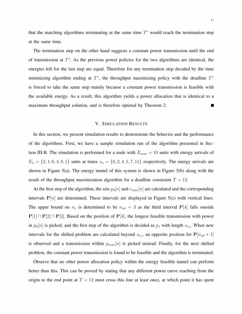
of the algorithms. First, we have a sample simulation run of the algorithm presented in Sec-
tion III-B. The simulation is performed for a node with Emax = 10 units with energy arrivals of
En = {2, 1, 6, 4, 8, 1} units at times sn = {0, 2, 4, 5, 7, 11} respectively. The energy arrivals are
shown in Figure 5(a). The energy tunnel of this system is shown in Figure 5(b) along with the
result of the throughput maximization algorithm for a deadline constraint T = 12.
At the first step of the algorithm, the sets p0[n] and rmax[n] are calculated and the corresponding
intervals P[n] are determined. These intervals are displayed in Figure 5(c) with vertical lines.
The upper bound on n1 is determined to be nub = 3 as the third interval P[4] falls outside
P[1]∩P[2]∩P[3]. Based on the position of P[4], the longest feasible transmission with power
in p0[n] is picked, and the first step of the algorithm is decided as p1 with length sn1 . When new
intervals for the shifted problem are calculated beyond sn1 , an opposite position for P[nub + 1]
is observed and a transmission within pmax[n] is picked instead. Finally, for the next shifted
problem, the constant power transmission is found to be feasible and the algorithm is terminated.
Observe that no other power allocation policy within the energy feasible tunnel can perform
better than this. This can be proved by stating that any different power curve reaching from the
origin to the end point at T = 12 must cross this line at least once, at which point it has spent
18
the same amount of energy while departing strictly less bits.
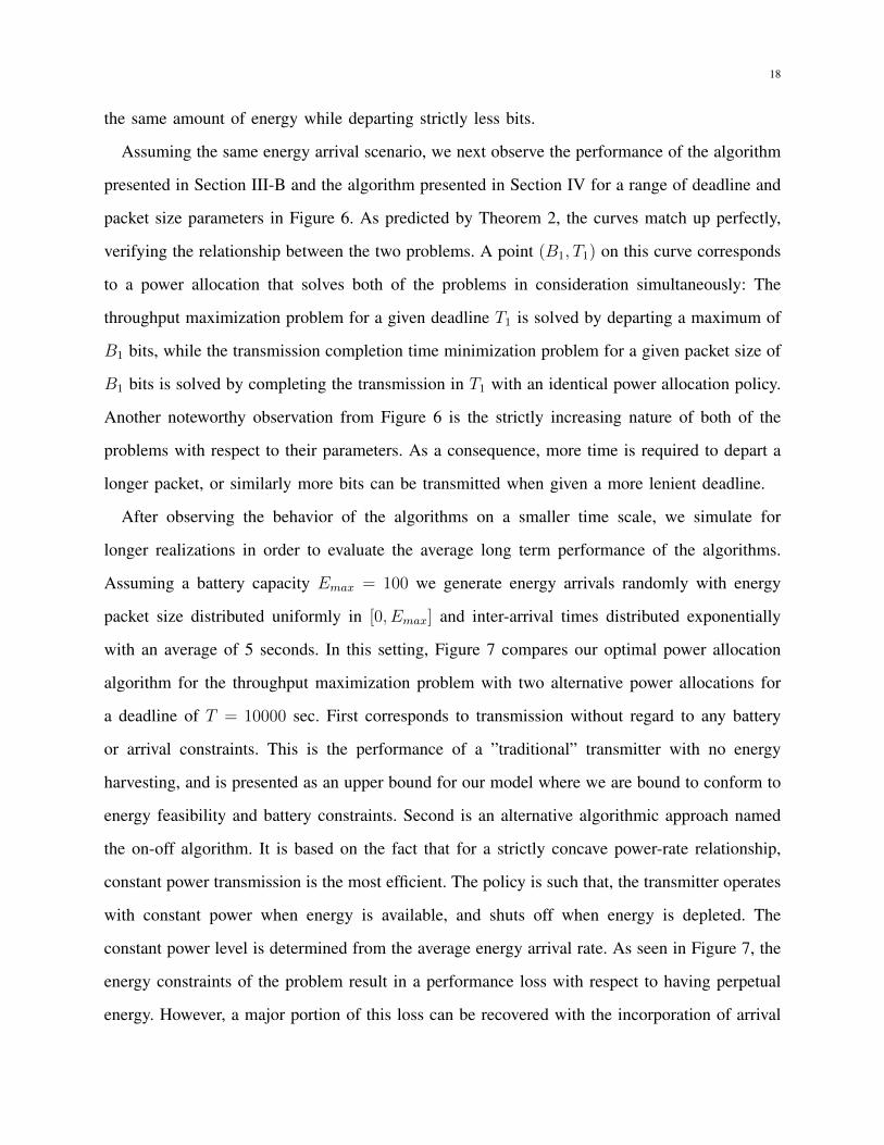
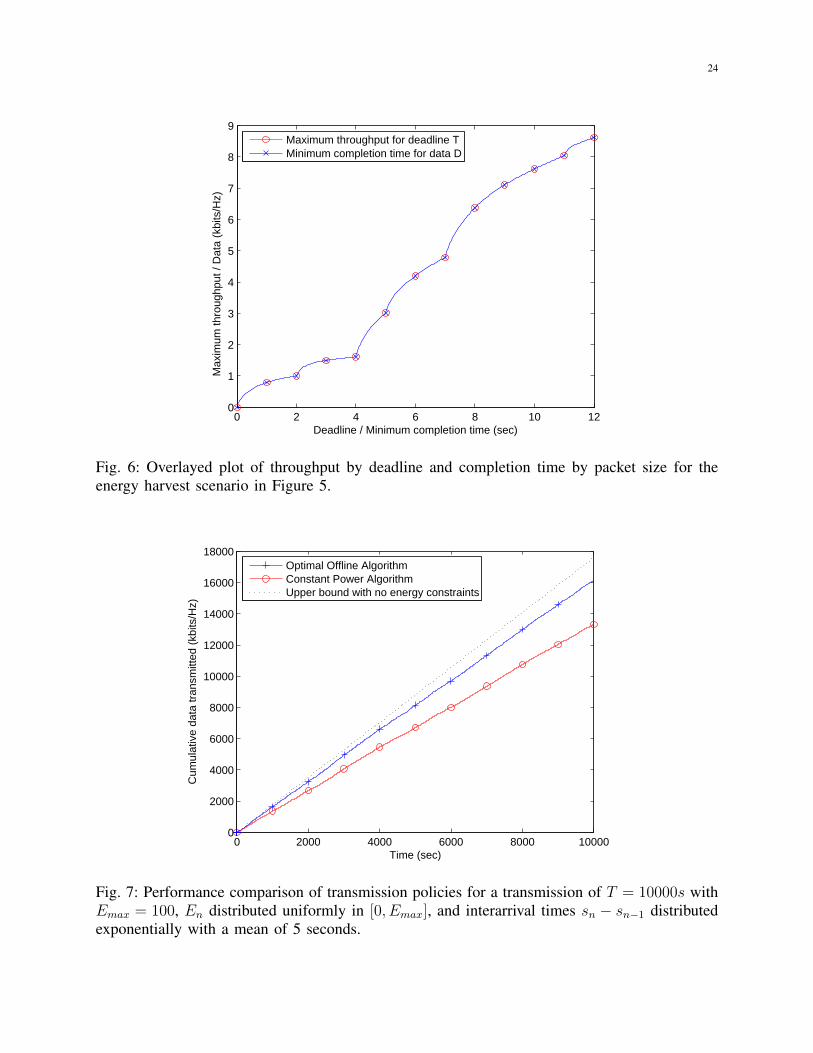
Assuming the same energy arrival scenario, we next observe the performance of the algorithm
presented in Section III-B and the algorithm presented in Section IV for a range of deadline and
packet size parameters in Figure 6. As predicted by Theorem 2, the curves match up perfectly,
verifying the relationship between the two problems. A point (B1, T1) on this curve corresponds
to a power allocation that solves both of the problems in consideration simultaneously: The
throughput maximization problem for a given deadline T1 is solved by departing a maximum of
B1 bits, while the transmission completion time minimization problem for a given packet size of
B1 bits is solved by completing the transmission in T1 with an identical power allocation policy.
Another noteworthy observation from Figure 6 is the strictly increasing nature of both of the
problems with respect to their parameters. As a consequence, more time is required to depart a
longer packet, or similarly more bits can be transmitted when given a more lenient deadline.
After observing the behavior of the algorithms on a smaller time scale, we simulate for
longer realizations in order to evaluate the average long term performance of the algorithms.
Assuming a battery capacity Emax = 100 we generate energy arrivals randomly with energy
packet size distributed uniformly in [0, Emax] and inter-arrival times distributed exponentially
with an average of 5 seconds. In this setting, Figure 7 compares our optimal power allocation
algorithm for the throughput maximization problem with two alternative power allocations for
a deadline of T = 10000 sec. First corresponds to transmission without regard to any battery
or arrival constraints. This is the performance of a ”traditional” transmitter with no energy
harvesting, and is presented as an upper bound for our model where we are bound to conform to
energy feasibility and battery constraints. Second is an alternative algorithmic approach named
the on-off algorithm. It is based on the fact that for a strictly concave power-rate relationship,
constant power transmission is the most efficient. The policy is such that, the transmitter operates
with constant power when energy is available, and shuts off when energy is depleted. The
constant power level is determined from the average energy arrival rate. As seen in Figure 7, the
energy constraints of the problem result in a performance loss with respect to having perpetual
energy. However, a major portion of this loss can be recovered with the incorporation of arrival
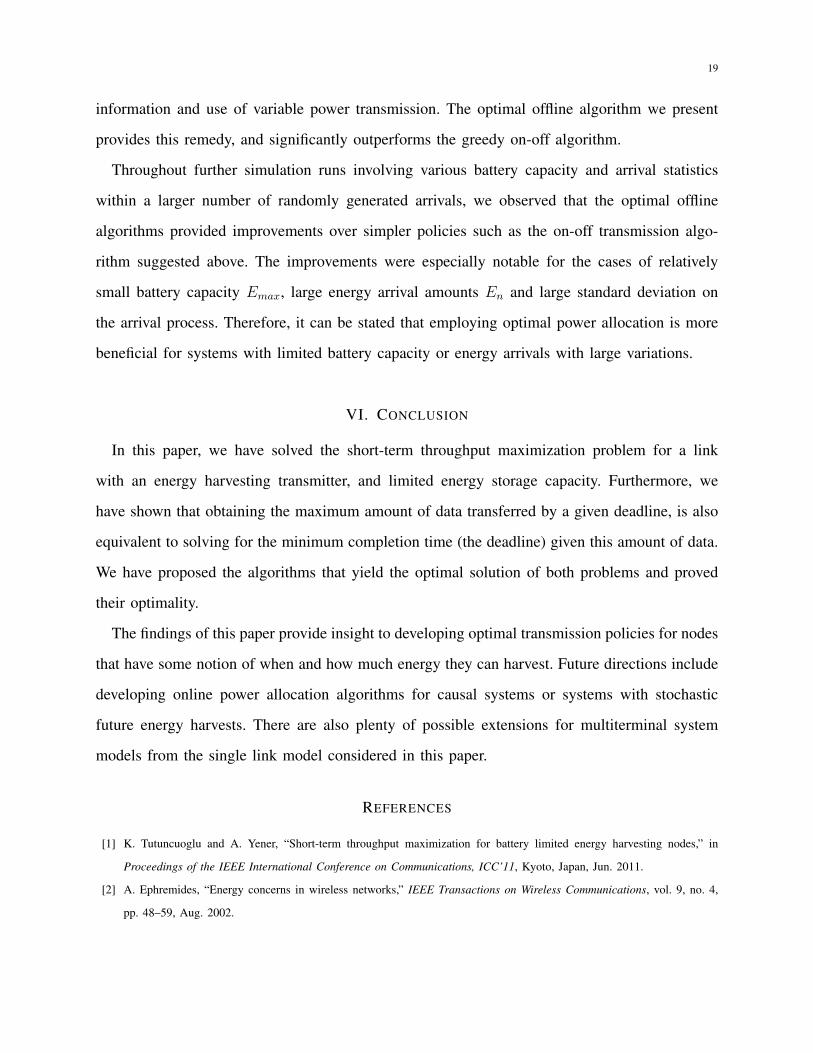
19
information and use of variable power transmission. The optimal offline algorithm we present
provides this remedy, and significantly outperforms the greedy on-off algorithm.
Throughout further simulation runs involving various battery capacity and arrival statistics
within a larger number of randomly generated arrivals, we observed that the optimal offline
algorithms provided improvements over simpler policies such as the on-off transmission algo-
rithm suggested above. The improvements were especially notable for the cases of relatively
small battery capacity Emax, large energy arrival amounts En and large standard deviation on
the arrival process. Therefore, it can be stated that employing optimal power allocation is more
beneficial for systems with limited battery capacity or energy arrivals with large variations.
VI. CONCLUSION
In this paper, we have solved the short-term throughput maximization problem for a link
with an energy harvesting transmitter, and limited energy storage capacity. Furthermore, we
have shown that obtaining the maximum amount of data transferred by a given deadline, is also
equivalent to solving for the minimum completion time (the deadline) given this amount of data.
We have proposed the algorithms that yield the optimal solution of both problems and proved
their optimality.
The findings of this paper provide insight to developing optimal transmission policies for nodes
that have some notion of when and how much energy they can harvest. Future directions include
developing online power allocation algorithms for causal systems or systems with stochastic
future energy harvests. There are also plenty of possible extensions for multiterminal system
models from the single link model considered in this paper.
REFERENCES
[1] K. Tutuncuoglu and A. Yener, “Short-term throughput maximization for battery limited energy harvesting nodes,” in
Proceedings of the IEEE International Conference on Communications, ICC’11, Kyoto, Japan, Jun. 2011.
[2] A. Ephremides, “Energy concerns in wireless networks,” IEEE Transactions on Wireless Communications, vol. 9, no. 4,
pp. 48–59, Aug. 2002.
20
[3] X. Jiang, J. Polastre, and D. Culler, “Perpetual environmentally powered sensor networks,” in Proc. 4th International
Symposium on Information Processing in Sensor Networks (IPSN), 2005, pp. 463–468.
[4] E. Uysal-Biyikoglu, B. Prabhakar, and A. El Gamal, “Energy-efficient packet transmission over a wireless link,” IEEE/ACM
Transactions on Networking, vol. 10, pp. 487–499, 2002.
[5] M. A. Zafer and E. Modiano, “A calculus approach to energy-efficient data transmission with quality-of-service constraints,”
IEEE/ACM Transactions on Networking, vol. 17, pp. 898–911, Mar. 2010.
[6] A. C. Fu, E. Modiano, and J. N. Tsitsiklis, “Optimal energy allocation and admission control for communications satellites,”
IEEE/ACM Transactions on Networking, vol. 11, no. 3, pp. 488–500, 2003.
[7] W. Heinzelman, A. Chandrakasan, and H. Balakrishnan, “An application-specific protocol architecture for wireless
microsensor networks,” IEEE Transactions on Wireless Communications, vol. 1, pp. 660–670, Oct. 2002.
[8] W. Ye, J. Heidemann, and D. Estrin, “An energy-efficient MAC protocol for wireless sensor networks,” in IEEE INFOCOM,
vol. 3, 2002, pp. 1567–1576.
[9] S. Bandyopadhyay and E. Coyle, “An energy efficient hierarchical clustering algorithm for wireless sensor networks,” in
IEEE INFOCOM, vol. 3, Mar. 2003, pp. 1713 – 1723.
[10] M. Adamou and S. Sarkar, “A framework for optimal battery management for wireless nodes,” in IEEE INFOCOM, vol. 3,
2002, pp. 1783–1792.
[11] E. Uysal-Biyikoglu and A. El Gamal, “On adaptive transmission for energy efficiency in wireless data networks,” IEEE
Transactions on Information Theory, vol. 50, pp. 3081–3094, Dec. 2004.
[12] P. Lettieri and M. B. Srivastava, “On adaptive transmission for energy efficiency in wireless data networks,” IEEE
INFOCOM, vol. 2, pp. 564–571, 1998.
[13] M. Gatzianas, L. Georgiadis, and L. Tassiulas, “Control of wireless networks with rechargeable batteries,” IEEE
Transactions on Wireless Communications, vol. 9, pp. 581–593, Feb. 2010.
[14] V. Sharma, U. Mukherji, V. Joseph, and S. Gupta, “Optimal energy management policies for energy harvesting sensor
nodes,” IEEE Transactions on Wireless Communications, vol. 9, no. 4, pp. 1326–1336, 2010.
[15] L. Lin, N. Shroff, and R. Srikant, “Asymptotically optimal power-aware routing for multihop wireless networks with
renewable energy sources,” IEEE/ACM Transactions on Networking, vol. 15, pp. 1021–1034, Oct. 2007.
[16] J. Lei, R. Yates, and L. Greenstein, “A generic model for optimizing single-hop transmission policy of replenishable
sensors,” Wireless Communications, IEEE Transactions on, vol. 8, no. 2, pp. 547–551, 2009.
[17] A. Seyedi and B. Sikdar, “Energy efficient transmission strategies for body sensor networks with energy harvesting,”
Communications, IEEE Transactions on, vol. 58, no. 7, pp. 2116–2126, 2010.
[18] D. Niyato, E. Hossain, and A. Fallahi, “Sleep and wakeup strategies in solar-powered wireless sensor/mesh networks:
Performance analysis and optimization,” IEEE Transactions on Mobile Computing, pp. 221–236, 2007.
[19] J. Yang and S. Ulukus, “Transmission completion time minimization in an energy harvesting system,” in 44th Annual
Conference on Information Sciences and Systems, Princeton, Mar. 2010.
[20] ——, “Optimal packet scheduling in an energy harvesting communication system,” Communications, IEEE Transactions
on, submitted June 2010, Available at http://arxiv.org/PS cache/arxiv/pdf/1010/1010.1295v1.pdf.
21
s10 s2 s3 s4 t
E0 E1 E2 E3 E4
Fig. 1: Energy harvesting model.
0 s1
p1
sn1t
P
sn1−1...
P[1] P[ ]n1
snn1
Fig. 2: Pictorial depiction of the behavior of feasible power ranges for future arrivals.
s1 s2
E1
E2
E0
0
E
t
EmaxP[2]
Fig. 3: The feasible energy tunnel.
22
sn1
E0
0
E
t
A
III
snub1
(a) Emax case
sn1
snub1
E0
0
E
t
B
IIIIV
(b) E0 case
Fig. 4: The optimal first step and suboptimal regions.
23
E0 E1 E2 E3 E4 E5
s1 s2 s3 s4 s50 t
0
0 sn1
p1
snub T
ET
snub1
t
t
P
(c)
(b)
(a)
Fig. 5: Arrival scenario and simulation results for the sample run.
24
0 2 4 6 8 10 120
1
2
3
4
5
6
7
8
9
Deadline / Minimum completion time (sec)
Max
imum
thro
ughp
ut /
Dat
a (k
bits
/Hz)
Maximum throughput for deadline TMinimum completion time for data D
Fig. 6: Overlayed plot of throughput by deadline and completion time by packet size for theenergy harvest scenario in Figure 5.
0 2000 4000 6000 8000 100000
2000
4000
6000
8000
10000
12000
14000
16000
18000
Time (sec)
Cum
ulat
ive
data
tran
smitt
ed (
kbits
/Hz)
Optimal Offline AlgorithmConstant Power AlgorithmUpper bound with no energy constraints
Fig. 7: Performance comparison of transmission policies for a transmission of T = 10000s withEmax = 100, En distributed uniformly in [0, Emax], and interarrival times sn − sn−1 distributedexponentially with a mean of 5 seconds.