Embed Size (px)
Citation preview
Option Valuation under Stochastic Volatility
With Mathematica Code
Copyright µ 2000 by Alan L. Lewis
All rights reserved. Except for the quotation of short passages for the purposesof criticism and review, no part of this publication may be reproduced, stored ina retrieval system, or transmitted, in any form or by any means, electronic,mechanical, photocopying, recording or otherwise, without the prior permissionof the publisher.
Reasonable efforts have been made to publish reliable data and information, butthe author and the publisher cannot assume responsibility for the validity of allmaterials or the consequences of their use. All information, including formulas,documentation, computer algorithms, and computer code are provided with nowarranty of any kind, express or implied. Neither the author nor the publisheraccept any responsibility or liability for the consequences of using them, anddo not claim that they serve any particular purpose or are free from errors.
Published by: Finance Press, Newport Beach, California, USACover design by: Brian Burton Design
For the latest available updates and corrections to this book and publishercontact information, visit the Internet sites:http:// www.financepress.com or http://members.home.net/financepress
Trademark notice: Mathematica is a trademark of Wolfram Research, Inc.,which is not associated with the author or publisher of this book.
International Standard Book Number 0-9676372-0-1Library of Congress Card Number: 99-91935
Printed in the United States of AmericaPrinted on acid-free paper
The Term Structure of Implied Volatility 177
6 The Term Structure of ImpliedVolatility
The term structure of implied volatility is the relation between the option
implied volatility and time to maturity: ( )impT U . Using our previous notation,
it’s the square root of ( , , )impV X V U , holding the moneyness X and the initialvolatility V fixed. In practice, the implied volatility is usually measured at a
strike price close to the money. ( X � � is a natural choice). In fact, thequalitative behavior is the same at any strike: a graph of ( )imp
T U vs. U
ultimately flattens to a limiting asymptotic value, /( )imp impVTd d�
� � , that is
independent of both X and V. This general behavior is analogous to the termstructure of interest rates and the existence of a long-run rate of interest.
The asymptotic implied volatility depends only upon the parameters of thevolatility process. It can be calculated from the simple relation
( )impV kMd
� �� ,
where M is the first eigenvalue of a differential operator, and k� is a complex
number. We illustrate 3 ways to calculate impVd
for general models: a seriesmethod, a variational method, and a differential equation-based method.Computation times for the latter two methods are just a couple of seconds in
Mathematica.
178 Option Valuation Under Stochastic Volatility
1 Deterministic Volatility
The volatility models that we consider in this book typically have a similar
structure: ( ) ( )t t t tdV b V dt a V dW� � , where the drift term ( )tb V exhibits mean-reversion. For example, the GARCH diffusions and other models have the lineardrift form ( )t tb V VX R� � , where X and R are positive constants. If the
volatility becomes small, then ( )tb V is positive, causing the volatility to tend togrow larger. If the volatility is large, then ( )tb V is negative, causing the volatilityto tend to grow smaller.
To a first approximation, the term structure is explained by letting the Browniannoise term vanish1. For the linear drift models, we are left with the deterministic
volatility evolution t tV VX R� �� , where the dot means a time derivative. Thesolution to the differential equation y yX R� �� , where ( )y V�� is given by
(6.1) ( , ) ( ) ty t V V e RX X
R R
�
� � � .
In (6.1), the behavior is especially simple as tld ; no matter what thestarting value V, the volatility tends to the fixed point * /V X R� . This value is
called a fixed point because if the volatility starts there, it stays there. The fixedpoint is attractive or stable because small departures of the volatility from V*are damped over time.
Option valuation under deterministic volatility is a well-known application ofthe B-S theory. Options are still priced by the B-S formula, but the volatility
parameter in the formula is modified. The modified volatility is simply the time-average of the deterministic volatility. In other words, if ( , , )C S V U is the generalcall option value and ( , , )c S V U is the B-S value, then under deterministic
volatility:
1 For simplicity, we call the term structure of implied volatility just the term
structure. With the exception of one subsection, in this chapter the risk-adjustedvolatility process and the actual volatility process are assumed identical (a risk-neutral world). See Chapter 8 (Duality and Changes of Numeraire) to convert
the results in this chapter to log-utility.
The Term Structure of Implied Volatility 179
(6.2) ( , , ) , ( , ),C S V c S VU N U U� ,
where ( , ) ( , ) eV y s V ds VRUU X XN U
U R R RU
�� ¬� �� � � � � �� ®¨�
� � .
The B-S implied volatility is given by /( , )] [ ( , )]imp V VT U N U� � � .
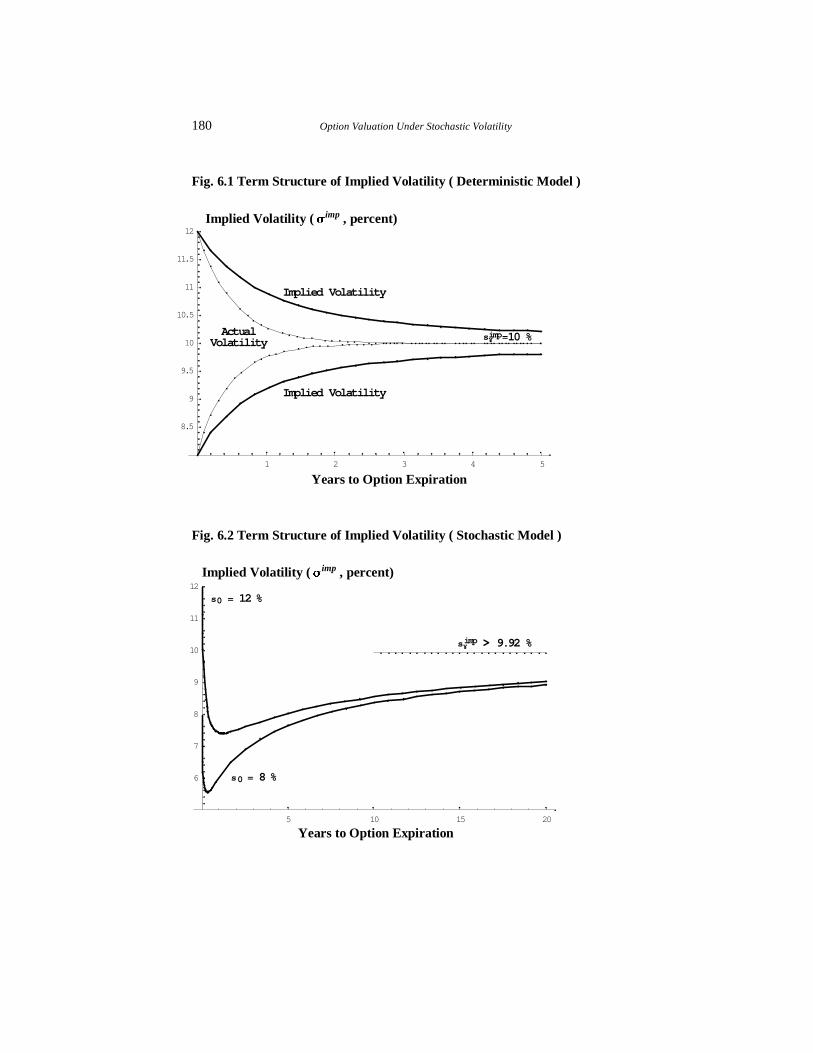
Shown in Fig. 6.1 is a plot of both ( , )imp VT U and /[ ( , )]y VU � � versus U , where.aX � � �� and aR � � , (annualized parameters). We show two cases: (i) initial
volatility %aT � � ( . )aV � � ���� and (ii) initial volatility%aT � �� ( . )aV � � ���� . Notice that the implied volatility (the bold line)
behaves a lot like the actual volatility ( , )y VU (the thin line); the only difference
is that the implied volatility changes more slowly because it’s a time-average.But both functions begin at V and evolve in a smooth monotonic fashion with alimiting asymptotic value /( / ) %impT X R
d� �� �
�� . The asymptotic value is
independent of the starting value V, as well as , , ,S K r and E .
The rate of convergence to the asymptotic value is determined by the parameter
R , which has the dimensions [ / ]U� . Since the “decay rate” is determined by theexponential term exp( )RU� , this type of behavior is often described as having a“half-life” / /U R�� � � . In our example, / .U �� � � � years and one can see from
Fig 6.1 that both the actual and implied volatilities have moved, very roughly,about half-way toward their final asymptotic value at .U � � � years.
Many other models of interest to researchers have a deterministic limit thatbehaves in the same way as this example. In general, volatility evolution in thedeterministic limit is ( )t tV b V�� , where ( )b ¸ is the drift coefficient. If a model is
mean-reverting, ( )b V will typically have a single zero at some *V V� . Thezero will be attractive, meaning not only ( *)b V � � but also ( *)b Va � � , wherethe prime means a derivative. If you picture the graph of ( )tb V you can see that
the volatility evolution will be similar to Fig. 6.1. It follows from ( )t tV b V��
that ( )b V has the dimensions of [ / ]V t , so that ( *)b Va has the dimensions[ / ]t� . This causes | / ( *) |b Va� to play the role of the half-life parameter in
general models, at least asymptotically.
180 Option Valuation Under Stochastic Volatility
Fig. 6.1 Term Structure of Implied Volatility ( Deterministic Model )
Implied Volatility (Timp , percent)
Years to Option Expiration
Fig. 6.2 Term Structure of Implied Volatility ( Stochastic Model )
Implied Volatility (Timp , percent)
Years to Option Expiration5 10 15 20
6
7
8
9
10
11
12
s¥imp > 9.92 %
s0 = 12 %
s0 = 8 %
1 2 3 4 5
8.5
9
9.5
10
10.5
11
11.5
12
ActualVolatility
Implied Volatility
Implied Volatility
s¥imp=10 %
The Term Structure of Implied Volatility 181
2 Deterministic Volatility II: a TransformPerspective
In the last section we showed that the deterministic volatility model
t tV VX R� �� has an asymptotic implied volatility /impV X Rd
� . In this section
we consider this same problem with the transform method. The advantage of thetransform method is that it also solves the case we are really interested in—stochastic volatility.
Call option Solution II of (2.2.10) is:
(2.1) ˆ ( , , )
( , , )i
i
ik
r ikX
ik
H k VC S V Se Ke e dk
k ikEU U U
UQ
�d
� � �
�d
� ��¨ �
�
�, Im k� �� � .
The natural strike price K at which to measure the term structure is given byX � � , which corresponds to rKe SeU EU� �� . If r Ev and you measure atK S� , you are systematically moving to one side of the volatility smile
pattern as the time to expiration increases. With the better choice X � � , (2.1)simplifies to:
(2.2) ˆ ( , , )( , , )
i
i
ik
rik
H k VC S Vdk
Ke k ikU
UU
Q
�d
�
�d
� ��¨ �
��
�
We established in Chapter 2 that, under constant volatility, this solution was
valid for the entire strip Im k� �� � . The same holds true under deterministicvolatility because, as we will show, ˆ ( , , )H k V U is an entire function under eitherconstant or deterministic volatility.
We established the solution for the fundamental transform ˆ ( , , )H k V U underdeterministic volatility in Appendix 3.1 at (3.A.2). For the drift function
( )b V VX R� � , that formula becomes
< >( )ˆ ( , , ) exp ( ) ( , )H k V c k U VU U� �� , where ( ) ( )c k k ik� ���
�,
and ( , ) ( , ) eU V y s V ds VRUU
X XU U
R R R
�� ¬� �� � � � � �� ®¨�
� .
This shows that ( )ˆ ( )H k� is an entire function of k in the complex k-plane. A
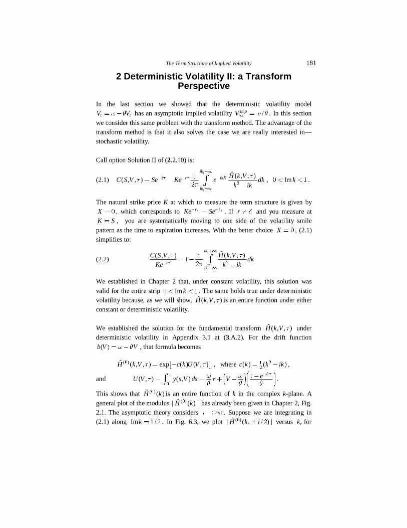
general plot of the modulus ( )ˆ| ( ) |H k� has already been given in Chapter 2, Fig.2.1. The asymptotic theory considers U ld . Suppose we are integrating in(2.1) along Im /k � � � . In Fig. 6.3, we plot ( )ˆ| ( / ) |rH k i��
� versus rk for
182 Option Valuation Under Stochastic Volatility
, , and U � � �� ��� years, using the previous numerical example .aX � � �� ,
aR � � , and .aV � � ���� .
Fig. 6.3. ˆ| |H� �N along an Integration Contour (Im 1/2)k Various Times to Maturity U (Deterministic Model)
ˆ| |H
Re k
As you can see from Fig. 6.3, the fundamental transform becomes increasinglypeaked about rk � � as the time to maturity increases. For U �� � , (2.2)becomes
( , , )exp ( ) ( )
i
i
ik
rik
dkC S Vc k c k V
Ke k ikUU
U X XU
Q R R R
�d
�ld
�d
¯x � � � �¡ °
¢ ± �¨ �
� ��
�
Of course because this is the B-S theory, we could evaluate this integral exactly(see Chapter 2, Appendix 1). But an alternative method will also work in thestochastic volatility case: the asymptotic method of steepest descent.2 As
U ld , Fig. 6.3 shows that the exponential factor in the integral damps thecontribution everywhere except near rk � � , which is our integration origin. If
2 For a nice discussion of the methods of steepest descent, saddle points, and themethod of stationary phase, see Carrier, Krook, and Pearson (1966, Chapt. 6).
-10 -5 0 5 10
0
0.2
0.4
0.6
0.8
1
t=5 yrs
t=20 yrs
t=100 yrs
The Term Structure of Implied Volatility 183
we didn’t know this point, we could find it by looking for the stationary pointk� determined by '( )c k �� � , which has the solution /k i�� � . This solutionk� is also a saddle point because, while the modulus ˆ| |H is decreasing in thereal direction, it’s increasing in the imaginary direction (see Fig. 2.1 in Chapter
2). Along this integration contour, ( ) / /rc k k� � �� � � . This is an exact relation,
but in the stochastic case (see below), we will expand the integrand in a Taylorseries about the saddle point. In this special case, the Taylor series only has the
two terms. The leading asymptotic contribution to the integral is given by
( , , )exp exp exp r rr
C S VV k dk
Ke UU
U X X XU U
Q R R R R
d
�ld
�d
¯x � � � � �¡ °
¢ ± ¨�� �
�� � � �
The integral that remains is just a Gaussian
exp r rk dkX QRU
R XU
d
�d
� �¨ � �
�.
So we obtain the result
( , , )exp exp
r
C S VV
Ke UU
U R X XU
QXU R R R�ld
¯x � � � �¡ °
¢ ±
� ��
� �.
This result can be compared with the Black-Scholes formula, which is easily
shown to be, in this limit,
(2.3) ( , , )exp
r
c S V VVKe U
U
UU
Q U�ld
x � ��
��
.
Comparing the last two equations implies that /impV X Rd
� , just as we expected.
The important idea is that we now have a method for the stochastic case.
3 Stochastic Volatility—The EigenvalueConnection
Notice that as U ld , the fundamental transform in the previous section hadthe following special form
< > < >( )ˆ ( , , ) exp ( ) ( , ) exp ( ) ( , )H k V c k U V k u k VU
U U M Uld
� � x �� ,
where
( ) ( )k c k XM
R� and ( , ) exp ( )u k V c k V X
R R
¯� � �¡ °
¢ ±
� .
184 Option Valuation Under Stochastic Volatility
This form is special because, first of all, the dependence upon V and U hasseparated into the product of two terms, one depending upon U and one
depending upon V . (Both terms depend upon k) . Suppose, that under stochasticvolatility, the same form of solution holds:
(3.1) < >ˆ ( , , ) exp ( ) ( , )H k V k u k VU
U M Uld
x �
with new functions ( )kM and ( , )u k V to be determined. If we substitute thisform into the PDE (2.2.19) satisfied by the fundamental transform, then we areleft with the ordinary differential equation for ( , )u k V :
This is an eigenvalue equation, where ( )kM is an eigenvalue of the differential
operator k$ , and u is the associated eigenfunction.3. In general, there can bemany solutions to (3.2). In fact, you may be able to develop the fundamentaltransform at all times U (not just U ld ) as a sum over such solutions—this is
called an eigenfunction expansion4. But, in the limit U ld , the dominant termof such a sum uses the smallest or first eigenvalue. This may seem confusing atthis point because there are a lot of complex numbers appearing in (3.2), so what
do we mean by smallest? Below, we show that, in fact, everything we calculateis real-valued and the first or smallest eigenvalue is well-defined.
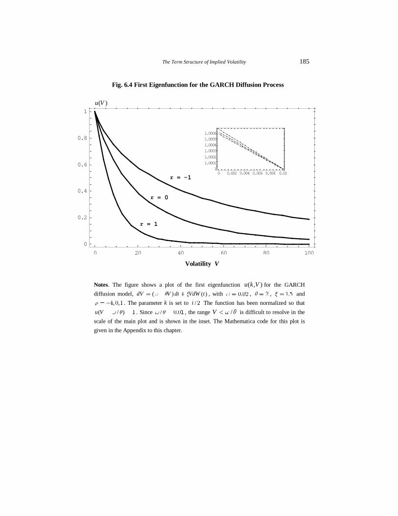
What does the first eigenfunction look like? In Fig. 6.4 we show plots of( , )u k V vs. V with /k i� � . The model is the GARCH diffusion process
( ) ( )dV V dt VdW tX R Y� � � , with .X � � �� , R � � , .Y � � � and
, ,S ��� � � . How we calculated that function is explained in Sec. 8.
3Eigenvalue problems are not well-defined until we specify a class of admissible
functions. This is discussed later in Sec. 74 See my article (Lewis 1998).
(3.2) ( )k u k uM�$ ,where
/( ) ( ) ( ) ( ) ( )kd u duu a V b V ik V a V V c k V u
dVdVS ¯� � � � �¢ ±
�� � ��
� �
�$ .
The Term Structure of Implied Volatility 185
Fig. 6.4 First Eigenfunction for the GARCH Diffusion Process
( )u V
Volatility V
Notes. The figure shows a plot of the first eigenfunction ( , )u k V for the GARCH
diffusion model, ( ) ( )dV V dt VdW tX R Y� � � , with .X � � �� , R � � , .Y � � � and
, ,S ��� � � . The parameter k is set to /i � The function has been normalized so that
( / )u V X R� � � . Since / .X R � � �� , the range /V X R� is difficult to resolve in the
scale of the main plot and is shown in the inset. The Mathematica code for this plot is
given in the Appendix to this chapter.
0 20 40 60 80 100
0
0.2
0.4
0.6
0.8
1
0 0.002 0.004 0.006 0.008 0.011
1.0001
1.0002
1.0003
1.0004
1.0005
1.0006
r = 1
r = 0
r = -1
186 Option Valuation Under Stochastic Volatility
With this general form of solution, then (2.2) becomes in the stochastic case:
(3.3) < >( , , )
exp ( ) ( , )i
i
ik
rik
dkC S Vk u k V
Ke k ikUU
UM U
Q
�d
�ld
�d
x � ��
¨ �
��
�,
The Ridge Property. Suppose that ( )kM has a saddle point k� in the complex
k-plane determined by the solution to ( )kM a �� � . We showed in Chapter 2 thatthe fundamental transform is often an analytic characteristic function. As weexplained in that chapter, analytic characteristic functions have the ridge
property, which means that any saddle point must lie along the purelyimaginary axis. In other words, k iy�� � , where y� is a real number. Thissaddle point location will be confirmed in computational examples below.
The reality of the eigenvalue problem (3.2). Recall the reflection property
from (2.2.20): *ˆ ˆ( , , ) ( *, , )H k V H k VU U� � . Combining this property with the
ridge property, any saddle point must be found along k iy� , where*ˆ ˆ( , , ) ( , , )H iy V H iy VU U� . That is: the fundamental transform is real along the
imaginary k-axis. In turn, this shows that both the first eigenvalue and the
associated eigenfunction are real along the imaginary axis. And finally, we can
see from (3.2) that each of the coefficients of the equation will be real along that
axis. In other words, to summarize: the asymptotic term structure is determined
by the smallest solution to an eigenvalue problem, where the eigenvalue,
eigenfunction, and associated PDE are all real-valued.5
An important element of the saddle point method is moving the integration
contour so that it traverses the saddle point. Before we can do that, recall that(3.3) is a valid formula as long as the integration contour lies in the intersectionof the fundamental strip Im kB C� � with the strip Im k� �� � ; this is the
strip of regularity. We now make the further assumption that the saddle pointImik k y� � � lies within the strip of regularity6. If it does, then, by Cauchy’s
theorem (See Chapter 2, Appendix 1), we can move the integration contour to
5 The complex-valued coefficients in (3.2) are needed for the full transform, butnot for its asymptotic saddle point behavior.6 Practical numerical examples—see Table 6.1—show that y� is often close to1/2, so this is not problematic in my experience.
The Term Structure of Implied Volatility 187
Imk y� � without changing the value of the integral. Next, expand ( )kM in a
Taylor series about k� :
( ) ( ) ( ) ( )r rk k k k k kM M M Maa� � � ��� � ��
� ,
so (3.3) becomes
< >( , , ) ( , )
exp ( ) exp ( )r rr
C S V u k Vk k k dk
Ke k ikUU
UM U M U
Q
d
�ld
�d
¯aax � � �¢ ±� ¨ �� �� ���
� �
��
�.
Note that this last integral is over a real integration variable. We know( )kM aa p� � because of the ridge property. Performing the integral gives us
(3.4) < >( , , ) ( , )
exp ( )( )r
C S V u k Vk
Ke k ik kUU
UM U
QM U�
ld
x � �aa�
���
� � �
��
�
.
Notice that the denominator term ( )k ik y y� � � ��
� � � �� � since, byassumption y� ��� � . The arbitrage bound ( , , )C S V Se EU
U�b combined with
rKe SeU EU� �� , implies that in (3.4) we must have ( , , ) / rC S V Ke UU
� b� . This
implies that not only is ( , )u k V� real, but it’s non-negative as well. That samebound also strengthens the inequality ( )kM aa p� � to ( )kM aa �� � . Finally,comparing (3.4) with (2.3) yields a simple result for the (at-the-money)
asymptotic implied volatility:
( ) ( )impV X kMd
� � �� �
Next, we repeat the calculation for an arbitrary value for the moneyness measureX. In that case, (3.4) becomes:
(3.5) < >( , , ) ( , )
exp ( )( )
Xr
C S V u k Ve k ik X
Ke k ik kU U
UM U
QM U�
ld
x � � �aa�
�� ��
� � �
�
�
.
But the B-S solution, for general X , has the asymptotic form:
(3.6) ( , , )expX
r
c S V Xe VV VKe U U
UU
Q U U�
ld
¯¡ °x � � �¡ °¢ ±
�
� �
� �
� .
Comparing the two solutions (3.5) and (3.6) implies that
(3.7) ( )imp
imp
X V k ik XV U
U M U
U ld
� ¬�� � x � �� �� ®
�
� �� �� �
After some rearrangement, (3.7) is equivalent to
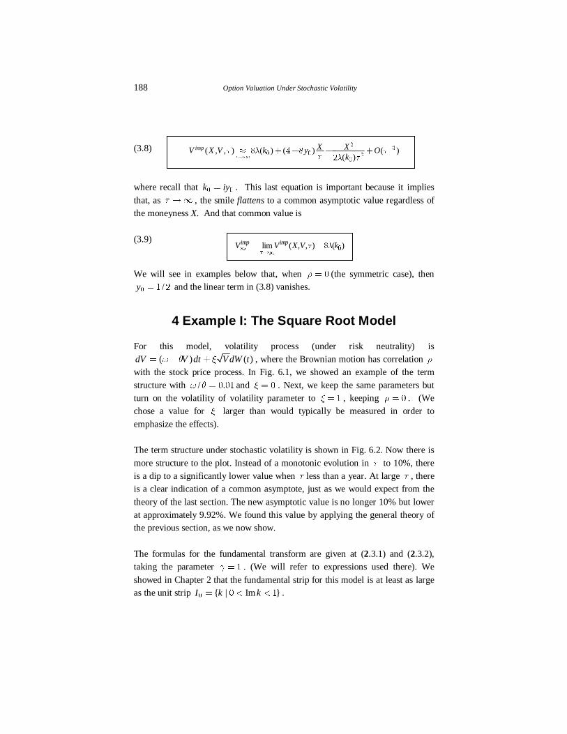
188 Option Valuation Under Stochastic Volatility
(3.8)
where recall that k iy�� � . This last equation is important because it implies
that, as U ld , the smile flattens to a common asymptotic value regardless ofthe moneyness X. And that common value is
(3.9)
We will see in examples below that, when S � � (the symmetric case), then/y �� � � and the linear term in (3.8) vanishes.
4 Example I: The Square Root Model
For this model, volatility process (under risk neutrality) is( ) ( )dV V dt V dW tX R Y� � � , where the Brownian motion has correlation S
with the stock price process. In Fig. 6.1, we showed an example of the term
structure with / .X R � � �� and Y � � . Next, we keep the same parameters butturn on the volatility of volatility parameter to Y � � , keeping S � � . (Wechose a value for Y larger than would typically be measured in order to
emphasize the effects).
The term structure under stochastic volatility is shown in Fig. 6.2. Now there is
more structure to the plot. Instead of a monotonic evolution in U to 10%, thereis a dip to a significantly lower value when U less than a year. At large U , thereis a clear indication of a common asymptote, just as we would expect from the
theory of the last section. The new asymptotic value is no longer 10% but lowerat approximately 9.92%. We found this value by applying the general theory ofthe previous section, as we now show.
The formulas for the fundamental transform are given at (2.3.1) and (2.3.2),taking the parameter H � � . (We will refer to expressions used there). We
showed in Chapter 2 that the fundamental strip for this model is at least as largeas the unit strip { | Im }I k k� � �� � � .
( , , ) ( ) ( ) ( )( )
imp X XV X V k y OkU
U M UU M U
�
ld
x � � � ��
�
� � �
�
� � ��
lim ( , , ) ( )imp impV V X V kU
U Md
ld
� � ��
The Term Structure of Implied Volatility 189
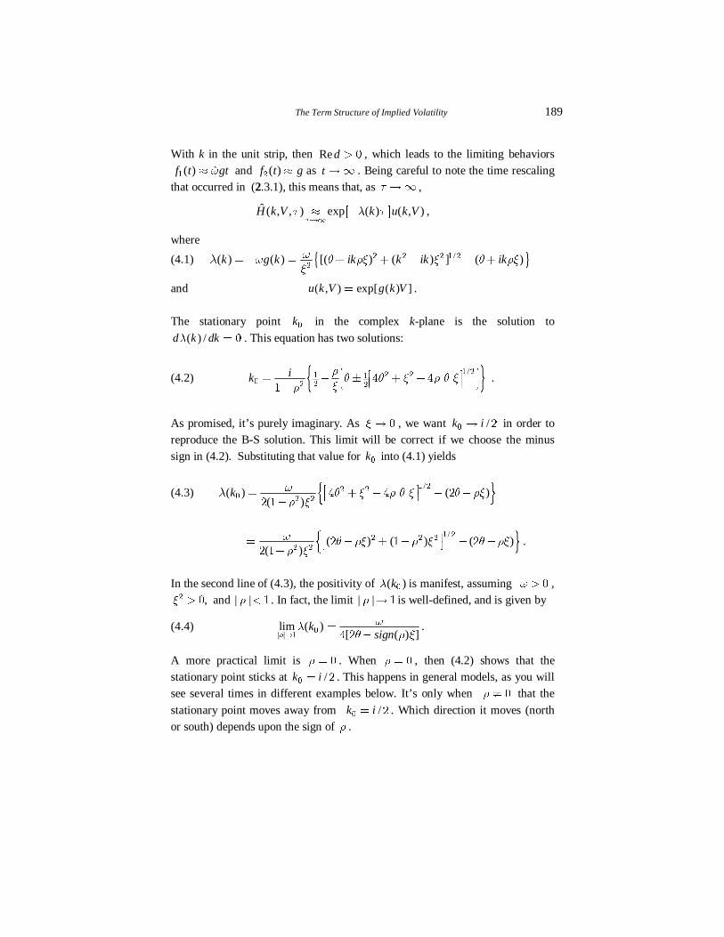
With k in the unit strip, then Re d � � , which leads to the limiting behaviors( )f t gtXx� � and ( )f t gx� as t ld . Being careful to note the time rescaling
that occurred in (2.3.1), this means that, as U ld ,
< >ˆ ( , , ) exp ( ) ( , )H k V k u k VU
U M Uldx � ,
where
(4.1) \ ^/( ) ( ) [( ) ( ) ] ( )k g k ik k ik ikXM X R SY Y R SYY
�� � � � � � �� � � � �
�
and ( , ) exp[ ( ) ]u k V g k V� .
The stationary point k� in the complex k-plane is the solution to
( ) /d k dkM � � . This equation has two solutions:
(4.2) \ ^/ ik
SR R Y S R Y
YS
� ¬� � � �� ® ¯� � o � �¡ °¢ ±�
� �� �� �� �� �
� ��
.
As promised, it’s purely imaginary. As Y l � , we want /k il� � in order toreproduce the B-S solution. This limit will be correct if we choose the minussign in (4.2). Substituting that value for k� into (4.1) yields
(4.3) \ ^/( ) ( )
( )k XM R Y S R Y R SY
S Y ¯� � � � �¢ ±�
� �� �
� � �� � �
� �
\ ^/( ) ( ) ( )
( )X R SY S Y R SYS Y
¯� � � � � �¢ ±�
� �� � �
� �� � �
� �.
In the second line of (4.3), the positivity of ( )kM � is manifest, assuming X � � ,,Y ��� and | |S � � . In fact, the limit | |S l � is well-defined, and is given by
(4.4) | |lim ( )
[ ( ) ]k
signS
XMR S Yl
��
�� � �
.
A more practical limit is S � � . When S � � , then (4.2) shows that thestationary point sticks at /k i�� � . This happens in general models, as you willsee several times in different examples below. It’s only when S v � that the
stationary point moves away from /k i�� � . Which direction it moves (northor south) depends upon the sign of S .
190 Option Valuation Under Stochastic Volatility
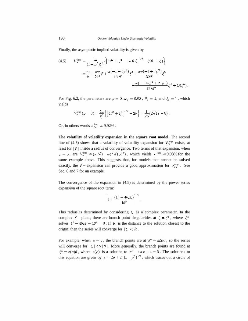
Finally, the asymptotic implied volatility is given by
(4.5) \ ^/ ( )
( )impV X R Y S R Y R SY
S Yd
¯� � � � �¢ ±�
� �� �
� �
�� � �
�
( )
XS X SX Y Y
R R R
� �� � �
��
� �
� �
� ��
( )XS SY
R
� ��
��
�
� �
��
( )
( )OX S S
Y YR
� �� �
� �� �
�
� �� ��
���.
For Fig. 6.2, the parameters are S � � , .aX � � �� , aR � � , and aY � � , whichyields
\ ^/( ) ( )impV XS R Y R
Yd
¯� � � � � �¢ ±
� �� �
�
� �� � � � �� �
��.
Or, in others words 9.92%impTd
! .
The volatility of volatility expansion in the square root model. The secondline of (4.5) shows that a volatility of volatility expansion for impV
d exists, at
least for | |Y inside a radius of convergence. Two terms of that expansion, whenS � � , are ( / ) /( )impV X R XY R
d! � � �
�� , which yields 9.93%impTd
! for thesame example above. This suggests that, for models that cannot be solved
exactly, the Y� expansion can provide a good approximation for impTd
. SeeSec. 6 and 7 for an example.
The convergence of the expansion in (4.5) is determined by the power seriesexpansion of the square root term:
/
( )Y RSY
R
¯�¡ °�¡ °¢ ±
� ��
�
��
�.
This radius is determined by considering Y as a complex parameter. In thecomplex Y� plane, there are branch point singularities at *Y Y� , where *Y
solves Y RSY R� � �� �� � � . If R is the distance to the solution closest to the
origin; then the series will converge for | | RY � .
For example, when S � � , the branch points are at * iY R� o� , so the series
will converge for | | | |Y R� � . More generally, the branch points are found at* ( )zY S R� , where ( )z S is a solution to z zS� � ��
� � � . The solutions tothis equation are given by / [ ]z iS S� o � � � �
� � � , which traces out a circle of
The Term Structure of Implied Volatility 191
radius 2 as S ranges from -1 to 1. Hence | | | |Y R� � is the radius of
convergence in the square root model for all | |S b � .
In Sec. 6, we develop the Y� expansion for impVd
for the GARCH diffusion—in
that case, we don’t know if the series converges in any radius.
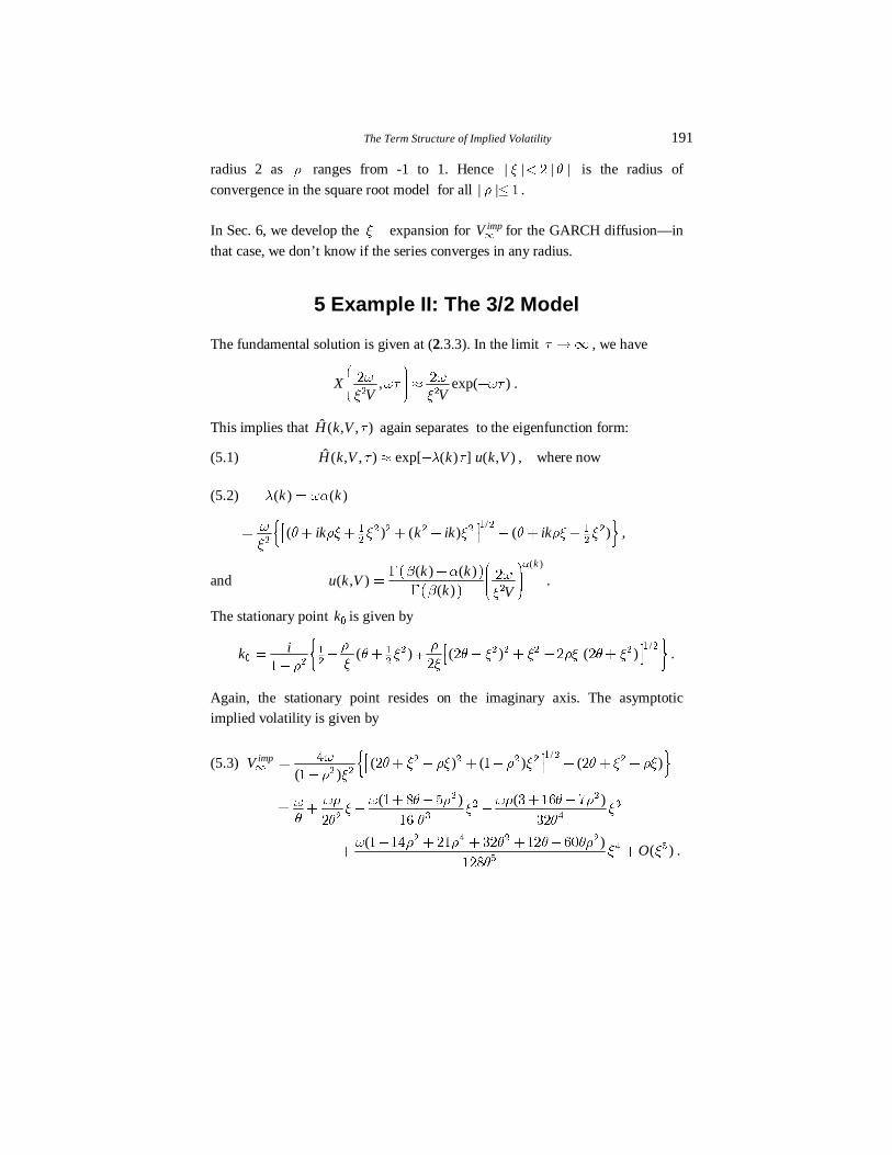
5 Example II: The 3/2 Model
The fundamental solution is given at (2.3.3). In the limit U ld , we have
, exp( )XV VX XXU XU
Y Y
� ¬� x �� �� ®� �
� � .
This implies that ˆ ( , , )H k V U again separates to the eigenfunction form:
(5.1) ˆ ( , , ) exp[ ( ) ] ( , )H k V k u k VU M Ux � , where now
(5.2) ( ) ( )k kM XB�
\ ^/( ) ( ) ( )ik k ik ikX R SY Y Y R SY Y
Y ¯� � � � � � � �¢ ±
� �� � � � �� �
� ��,
and
( )( ) ( )
( , )( )
kk k
u k Vk V
B
C B XC Y
� ¬( � �� � �( � ®�
� .
The stationary point k� is given by
\ ^/ ( ) ( ) ( )ik
S SR Y R Y Y SY R Y
Y YS� ¯� � � � � � �¢ ±�
� �� � � � �� �� � ��
� � ���
.
Again, the stationary point resides on the imaginary axis. The asymptoticimplied volatility is given by
(5.3) \ ^/( ) ( ) ( )
( )impV X R Y SY S Y R Y SY
S Yd
¯� � � � � � � �¢ ±�
� �� � � � �
� �
�� � �
�
( ) ( )
XS X R S XS R SX Y Y Y
R R R R
� � � �� � � �
� �� �
� � �
� � � � �� �
� �� ��
( )
( )OX S S R R RS
Y YR
� � � � �� �
� � � �� �
�
� �� �� �� �� ��
���.
192 Option Valuation Under Stochastic Volatility
It’s interesting that (5.3) may be obtained from (4.5) by making the substitution/R R Yl � �� in (4.5). The radius of convergence of (5.3) again vanishes with
R , but that radius has a more complicated dependence on parameters now.
6 Example III: The GARCH Diffusion Model
The GARCH diffusion model, under risk neutrality, has the volatility process
( ) ( )dV V dt VdW tX R Y� � � , so that the eigenvalue problem (3.2) becomes
(6.1) / ( ) ( )d u duV V ik V c k V u k udVdV
Y X R SY M ¯� � � � � �¢ ±
�� � � ��
� �
We don’t have an exact solution, so we need approximate methods. In this
section, we show one such method: the volatility of volatility series expansion.Previously, in Chapter 3, we showed how to use that expansion to develop thefull time dependence for the fundamental transform. Now, we don’t want the
time dependence—only the first eigenvalue solution to (6.1). There are twounknowns: the eigenfunction ( , )u k V and the first eigenvalue ( )kM .
It’s convenient to change variables from V to ( )x c k V� . While this wouldgenerally make x complex-valued, the solution we need resides on the purelyimaginary k-axis. That means it suffices to let k be purely imaginary and within
the strip Im k� �� � . With that restriction, ( )c k is a real, positive number andx is a real, positive number, just like V.
We let ( , ) ( )u k V f x� , where we will suppress the explicit k-dependence.Finally, introduce the new parameters ( )A c k X� , B R� , and
/ ( )D i k c kS� . All three parameters are real with k restricted as indicated.
With these changes, (6.1) becomes
(6.2) k f fM�$ , ( Im k� �� � , Re k � � )
where /k
d f dff x A Bx D x x f
dxdxY Y�� � � � �
�� � � ��
� �$ .
To create the series, substitute into (6.2) the formal expansions
( )j jM Y M� � , ( )( ) ( )j jf x f xY� �
For example, ( )f � satisfies
The Term Structure of Implied Volatility 193
(6.3) ( ) ( )
/ ( ) ( ) ( ) ( ) ( )df dfA Bx D x x f f f
dx dxY M M� � � � � �
� �
� � � � � � � .
When Y � � , we already have shown that
( ) ( )c k XMR
�� and ( ) exp ( )u c k V XR R
¯� � �¡ °¢ ±
� � .
In terms of the new variables, this translates into
( ) AB
M �� and ( ) ( ) exp ( *)f x x xB
¯� � �¡ °¢ ±� � , where * Ax
B� .
So (6.3) can be rewritten
(6.4) ( )
( ) ( ) ( )df
f h xdx B
� ��
� �� ,
where ( ) /
( ) ( ) exp ( *)
D xBh x x x
A B x B
M � ¯�� � �¡ °� ¢ ±
� � �
� � .
Now (6.4) is an ordinary differential equation with the general solution
(6.5) ( ) / / / ( )( ) ( )x
x B x B y B
xf x Ce e e h y dy� �� � ¨
�
� � ,
where C and x� are constants. The solutions to an eigenvalue equationf fM�$ are clearly determined only up to some constant multiplier. So we
need a normalization. Because ( ) ( *)f x x� ��� , we will enforce the
normalization ( *)f x x� � � . This means that ( ) ( *)if x x� � � for all i p � .Potentially, ( ) ( *)f x x� ��
� can be achieved by choosing C � � and
*x x�� in (6.5).
But (6.4) shows the integrand ( )h � has a denominator term that vanishes at
*x x� , so we have to be careful. We need an assumption: suppose/df dx exists at *x x� . Then, from (6.4) we see that ( ) /df dx� exists at
*x x� if and only if ( ) ( *)h x x�� exists (since ( ) ( *)f x ��� by the
normalization condition). By L’Hospital’s rule, ( ) ( *)h x x�� exists if thenumerator expression for ( ) ( )h x� also vanishes at *x x� . This determines
( )M � ; we must have
(6.6) /
( ) D AB B
M ��� �
� .
194 Option Valuation Under Stochastic Volatility
Then we can indeed take C � � , *x x�� and satisfy the normalization.Moreover, ( ) ( )f x� has now been determined:
(6.7) ( ) / / ( )
*( ) ( )
xx B y B
xf x e e h y dy�
� ¨� �
This basic argument works to all orders in the expansion. The general recursionsystem is, for , ,n � � �!
(6.8) ( ) / ( ) ( )
*
n n n
x x
d dD x f x fdx dx
M � �
�
¯� �¡ °
¡ °¢ ±
�� � � � ��
� �,
( ) / / ( )
*( ) ( )
xn x B y B n
xf x e e h y dy�� ¨ ,
( ) ( ) ( ) / ( ) ( )( )( )
nn j n j n n
j
d dh x f Dx f x fA Bx dx dx
M � � �
�
¯� ¡ °� � �
¡ °� ¡ °¢ ±�
�� � � � ��
� �
�
� ,
where terms with ( )n�� are omitted at n � � . Applying this algorithm, we find
(6.9) /
( )A A D A DB B B B
M Y Y� � � �� � �
� �
�� �
�
/
( )A D B A ADB B
Y� � � �� �
� � �
�� �� ��
��
( ) ( ) ( )[ ]A A D D B D OB
Y Y� � � � � ��
� � � � � �
�� � �� �� � ��
��
The stationary point must also be determined order by order in Y . We find
/ / ( )
( )k i OS X S RS S XX XY Y Y Y
R R RR R�
£ ¯ ²¦ ¦� � �¦ ¦¢ ±� � � �¤ »¦ ¦¦ ¦¥ ¼
� ��� � � �� � �
� � �
� �� ��
� � � ���
As expected, k� is pure imaginary. The stationary point sticks at /k i�� � ifS � � . Finally, the asymptotic implied volatility is given by
(6.10) ( )impV kMd � ��
/ /( ) [ ( ) ]
S X S S X S RX X XY Y Y
R R R RR R
� � � � �� � � �
� � � �� � � �� �
� �
� � �� �� �
� �� ��
[ ( ) ( )] ( )OX S S X R S Y YR
� � � � � � �� � � � � � � �
�
�� �� ��� � � ��
���.
The Term Structure of Implied Volatility 195
A dimensionality check. Recall the time dimensions for the GARCH diffusion
parameters: [ ] /[ ]V t� � , [ ] /[ ]tR � � , [ ] /[ ]tX �
�� , [ ] /[ ]tY �
�� . So if we write
( )impV gRd
� < , then ( )g < must be a function of dimensionless ratios. With only3 parameters with dimensions, there are only two independent ratios, so we must
have
,impV gYXRRR
d�
�.
Indeed, one can check that (6.10) is equivalent to
/( , ) ( )g x z x x z x zS S� � � � �� � � � �� �
� ��� �
/ / [( ) ] x x zS S� � � �� � � � � ��
���� �� �
[( ) ( ) ] ( )x x z O zS S S� � � � � � �� � � � � � ��
���� �� ��� � �� .
Numerical examples. We have extended (6.10) through ( )O Y�� , although theexpressions are too lengthy to report here. However, numerical examplesshowing the behavior of the partial sums through ( )O Y�� are given in Table 6.1.
As one sees, the series is fairly well-behaved for typical parameter values andthe partial sums tend to stabilize at higher order if R is not too small. The seriesresults are consistent with variational estimates, which are explained in the next
section.
196 Option Valuation Under Stochastic Volatility
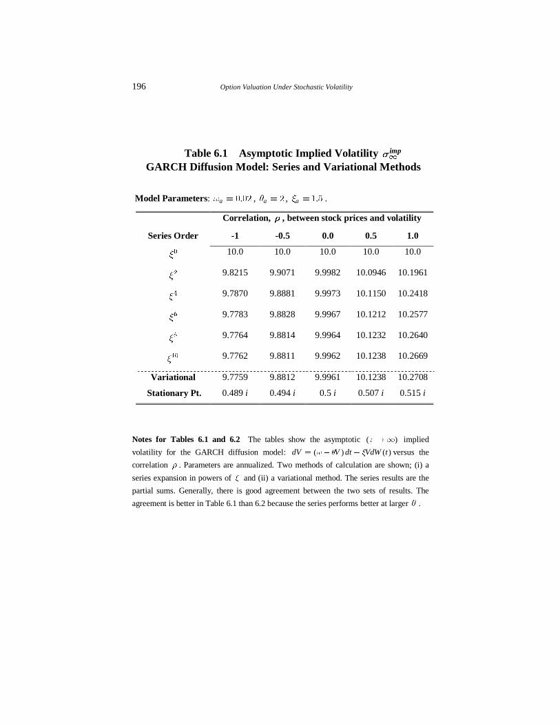
Table 6.1 Asymptotic Implied Volatility Td
imp
GARCH Diffusion Model: Series and Variational Methods
Model Parameters: .aX � � �� , aR � � , .aY � � � .
Correlation, S , between stock prices and volatility
Series Order -1 -0.5 0.0 0.5 1.0
Y� 10.0 10.0 10.0 10.0 10.0
Y� 9.8215 9.9071 9.9982 10.0946 10.1961
Y� 9.7870 9.8881 9.9973 10.1150 10.2418
Y� 9.7783 9.8828 9.9967 10.1212 10.2577
Y� 9.7764 9.8814 9.9964 10.1232 10.2640
Y�� 9.7762 9.8811 9.9962 10.1238 10.2669
Variational 9.7759 9.8812 9.9961 10.1238 10.2708
Stationary Pt. 0.489 i 0.494 i 0.5 i 0.507 i 0.515 i
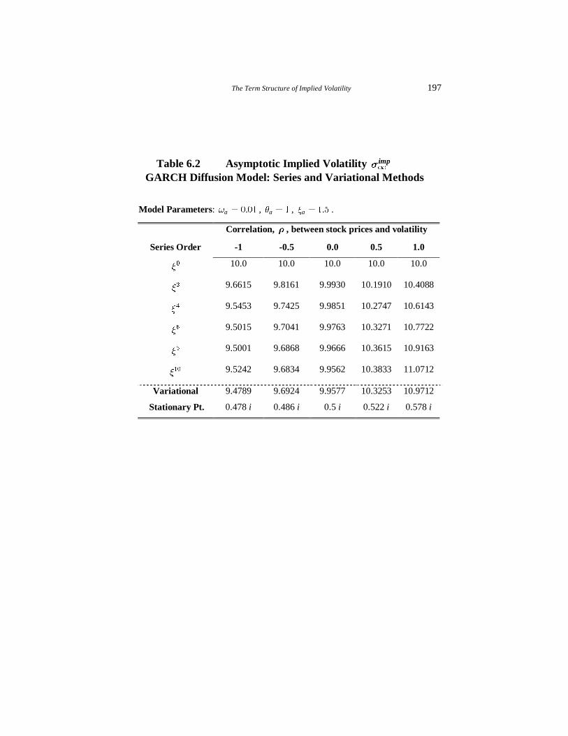
Notes for Tables 6.1 and 6.2 The tables show the asymptotic ( )U ld implied
volatility for the GARCH diffusion model: ( ) ( )dV V dt VdW tX R Y� � � versus the
correlation S . Parameters are annualized. Two methods of calculation are shown; (i) a
series expansion in powers of Y and (ii) a variational method. The series results are the
partial sums. Generally, there is good agreement between the two sets of results. The
agreement is better in Table 6.1 than 6.2 because the series performs better at larger R .
The Term Structure of Implied Volatility 197
Table 6.2 Asymptotic Implied Volatility Td
imp
GARCH Diffusion Model: Series and Variational Methods
Model Parameters: .aX � � �� , aR � � , .aY � � � .
Correlation, S , between stock prices and volatility
Series Order -1 -0.5 0.0 0.5 1.0
Y� 10.0 10.0 10.0 10.0 10.0
Y� 9.6615 9.8161 9.9930 10.1910 10.4088
Y� 9.5453 9.7425 9.9851 10.2747 10.6143
Y� 9.5015 9.7041 9.9763 10.3271 10.7722
Y� 9.5001 9.6868 9.9666 10.3615 10.9163
Y�� 9.5242 9.6834 9.9562 10.3833 11.0712
Variational 9.4789 9.6924 9.9577 10.3253 10.9712
Stationary Pt. 0.478 i 0.486 i 0.5 i 0.522 i 0.578 i
198 Option Valuation Under Stochastic Volatility
7 A Variational Principle Method
There is a deep connection between eigenvalue problems and variational
principles7. In this section, we make that connection for our application. Verybriefly, the first eigenvalue is a minimum of a certain functional. This extremalproperty can be exploited as a calculation tool, enabling the first eigenvalue
(and hence the asymptotic implied volatility) to be estimated to high accuracy.What makes our application special is the presence of the complex-valuedparameter k , a complication that requires careful handling.
We begin with the GARCH diffusion process of Sec. 6. After completing a fulltreatment including an example, we then extend the development to general
processes.
We gave the full time-development equation for the fundamental transform at
(2.2.19). With the volatility process given by the GARCH diffusion, we makethe same change of variables as in Sec. 6, letting ( )x c k V� , ( )A c k X� ,B R� , and / ( )D i k c kS� . In addition, we let ˆ ( , , ) ( , )H k V f xU U� , where
we imply the k-dependence. Then (2.2.19) becomes
(7.1) /k
f f ff x A Bx D x x f
xxY Y
U
s s s� � � � � � �
s ss
�
� � � ��
� �$ .
The k-plane restriction. Throughout this section, we take the parameter k to bepurely imaginary and restricted to the interval Im k� �� � . Because of thatrestriction, the new variable x is real and positive, and the coefficients in (7.1)
are all real. Because of the ridge property and the martingale property, thatrestricted interval in the complex k-plane suffices to determine the asymptoticimplied volatility for the option problem.
An auxiliary stochastic process. With our k-plane restrictions, (7.1) can beassociated with the real-valued, auxiliary stochastic process
(7.2) / ( )dx A Bx D x dt x dB tY Y� � � �� � , x� �d� ,
7 A classical and extensive reference is Courant and Hilbert (1989), Chapts IV
and VI.
The Term Structure of Implied Volatility 199
where ( )dB t is a Brownian motion. We use “auxiliary” because (7.2) is not
where we started. We began with the GARCH diffusion under risk neutrality,which is ( ) ( )dV V dt VdB tX R Y� � � —the auxiliary process has an extra termwith the D coefficient.
The forward equation. Next, consider the so-called “forward equation” for theauxiliary process:
(7.3) /( ) ( )p
p x p A Bx D x pxx
Y YU
s s s ¯� � � � �¢ ±s ss
c�
� � � ��
� �$ .
Our notation is that $ is the generator for the stochastic process (7.2) andc
$ is the formal adjoint. A time-independent solution to (7.3) is
(7.4) /( ) expB A D xp x xx
Y
YY
� �
¯¡ °� � �¡ °¢ ±
�� �
�
� �
We use the notation ( )p x to stress the positivity of the solution. When ( )p x
can be normalized, ( ( )p x dxd
¨ �d�
), it may be interpreted as the long-run
stationary probability distribution for the auxiliary process8. But we want toemphasize that the variational theory of this section does not require that
( )p x be integrable. The properties that are important are (i) ( )p x �c�$ and
(ii) ( )p x � � .
The variational principle. Recall the eigenvalue problem ( )k u k uM�$
defined at (6.2), where M is the first eigenvalue and u is the first eigenfunction.Multiply both sides by ( ) ( )u x p x and integrate by parts. Using ( )p x �c
�$ andsome algebra, you can establish the formula:
(7.5) < > < >\ ^
< >
( ) ( ) ( )
( ) ( )
p x x u x x u x dx
p x u x dx
YM
d
d
a ��¨
¨
� �� ��
��
�
�
if (i)$ the boundary terms from the parts integrations vanish:
,
lim ( ) ( ) ( )x
x p x u x u xl d
a ��
�
� ,
and (ii)$ all the integrals in (7.5) exist.
8 See Karlin and Taylor (1981, Chapter 15)
200 Option Valuation Under Stochastic Volatility
These are typical conditions associated with a variational method—let’s call(i)$ the endpoint conditions. We pointed out previously that ( )k u k uM�$ is not
well-defined until we specify a class of functions on which k$ acts. Differentclasses can give different eigenvalues. One natural class of functions for ourproblem is seen to be all twice differentiable functions ( )f x such that the
integrals in (7.5) exist and the endpoint conditions (i)$ hold. We call suchfunctions admissible and denote the set of all such function by $ , so (7.5)holds if u �$ .
The variational principle asserts that, for all ( )f x � $ , then
(7.6) < > < >\ ^
< >( )
( ) ( ) ( )min
( ) ( )f x
p x x f x x f x dx
p x f x dx
YM
d
d
�
£ ²¦ ¦a �¦ ¦¦ ¦¦ ¦� ¤ »¦ ¦¦ ¦¦ ¦¦ ¦¥ ¼
¨
¨
� �� ��
��
�
�
$
Specifically, a function ( )f x is admissible if
(i)$ ,
lim ( ) ( ) ( )x
x p x f x f xl d
a ��
�
� ,
and the integrals
(ii)$ ( )p x f dx¨ � , ( ) p x x f dx¨ � , ( ) ( )p x x f dxa¨ � �
are convergent. Note that the endpoint conditions do not require thateither ( )f x or ( )f xa individually exist at ,x � d� . As we stressed before, theintegrability conditions do not require that ( )p x itself be integrable. For
example, when D � � , then ( )p x is not integrable, but ( ) exp( )f x xB� � for
B� � is admissible. We use exactly this form in our computational examplebelow.
The variational principle (7.6) follows from the Euler-Lagrange equations ofthe theory of the calculus of variations. It’s a powerful tool that may be used to
estimate M to high accuracy by selecting suitable trial functions ( )f x . Ofcourse, a trial function should be admissible at the very least. In fact, foradmissible ( )f x , the inequality
(7.7) < > < >\ ^
< >
( ) ( ) ( )
( ) ( )
p x x f x x f x dx
p x f x dx
YM
d
d
a �b¨
¨
� �� ��
��
�
�
The Term Structure of Implied Volatility 201
is the tightest possible upper bound because it will be realized as an equality if
( )f x is chosen to be the first eigenfunction.
It’s interesting that in (7.7), the only explicit parameter that appears is Y� . Of
course, we know that the eigenvalue M depends upon the four parameters of theproblem: ,A B , D, and Y� or equivalently , , ,X R S and Y� . The other threeparameters have not disappeared, but are contained in ( )p x .
The case = 0S for the GARCH diffusion. Fig. 6.2 shows an example termstructure when S � � . Note how the asymptotic implied volatility, 9.92%, is
less than the deterministic value, 10%. While Fig. 6.2 is a plot of the square rootmodel, it suggests a result for the GARCH diffusion because the two modelsshare the same linear drift form. Indeed, the variational principle implies that,
when S � � , then impTd
never exceeds /( / )X R � � in the GARCH diffusion.Let’s see why.
We assume that X � � and R � � . If S � � , then D � � and ( )p x isnormalizable. In that case ( )f x � � is admissible and (7.7) implies that
( )
( ) ( )( )
p x xdx Ak c kp x dx B
XMR
¨
¨b � � .
The stationary point for ( )c k is /k i�� � , so we obtain( ) ( / ) / /( )k c iM X R X Rb �� � � . In other words, when S � � , then /impV X R
db .
�
When S v � , then /impV X Rd
� is possible. For example, the first two terms of
the Y� expansion for the GARCH diffusion at (6.10) are
/
( )impV OSX X Y Y
R R Rd
� � �� �
�
�,
and this will be larger than /X R for small Y and positive S . See Tables 6.1,
6.2 or Fig. 6.5 for more examples of /impV X Rd
� .
Numerical example. We continue with the GARCH diffusion for a numerical
example using the variational principle. Although we have suppressed the k-dependence in many formulas, to actually calculate, we need to reinstate it.More explicitly, (7.7) is a bound for ( )kM , where k iy� , y is real and in the
interval y� �� � . The weight function is more explicitly ( , )p k x , where
202 Option Valuation Under Stochastic Volatility
/
/ ( ) ( , ) exp
( )k ik i k xp k x x
x k ikR Y X S
YY
� �
£ ²¦ ¦ ¯�¦ ¦¦ ¦¡ °� � �¤ »¡ °¦ ¦�¢ ±¦ ¦¦ ¦¥ ¼
�
� ��
� �
� �
� � .
Let ( , ) ( , )p y x p iy x�� , a real positive function, given by
(7.8) /
/ ( ) ( , ) exp
( )y y xy
p y x xyx
R Y X S
YY
� �
£ ²¦ ¦ ¯�¦ ¦� � � ¡ °¤ »¦ ¦�¡ °¢ ±¦ ¦¥ ¼
�
� �
� �
�
� � �
�� .
Then, we can calculate the asymptotic implied volatility from
(7.9) < > < >\ ^
< >
( )
( , ) ( ) ( )max min
( , ) ( )
imp
y f x
p y x x f x x f x dxV
p y x f x dx
Yd
d d� �
�
£ ²¦ ¦a �¦ ¦¦ ¦¦ ¦b ¤ »¦ ¦¦ ¦¦ ¦¦ ¦¥ ¼
¨
¨
� �� ��
��
� � �
�
�
$
Note that its a maximum over y because the fundamental transform has a saddlepoint in the k-plane, which happens to have a maximum in the real direction anda minimum in the imaginary direction. So the fundamental transform has a
minimum as a function of y at the saddle point. But the eigenvalue affects thefundamental transform through a multiplicative term exp( )MU� ; that means weneed a maximum in the eigenvalue as a function of y.
Let’s check the consistency of these new ideas with the series solution of Sec. 6.Choosing a suitable trial function is something of an art. Your goal is to select a
function that is admissible, produces integrals that can be calculated, andcaptures the qualitative behavior of the first eigenfunction. For example, for theGARCH diffusion , we choose the trial function ( ) exp( )f x xB� � , where B
is a parameter which is optimized. This choice for the trial function is motivatedby the series solution ( ) exp( / )[ ( )]u x x OR Y� � �� . The integrals in (7.9) maybe computed by using
(7.10) / /exp ( )s d s K sN NNU U U
U
d� �� � �¨ � � � �
�
�� � ,
where ( )KN ¸ is the modified Bessel function of the second kind of order N . Inthis example, we find that (7.9) becomes
The Term Structure of Implied Volatility 203
(7.11) ( )
max min ( , , ) ( , , )( , , )
imp
ay
y yV g y a b g y a b
g y a b aN N
N
Y Ld � �
�� �
¯�b �¡ °
¡ °¢ ±
�
� ���� �
�,
using /( , , ) ( )!
n
nn
byg y a b K a
a na
N
N N
d
�
�
� � �
�
� � , and
XLY
��
�� , bS
XY
��
�, and RN
Y� �
�
�� .
In (7.11), the minimization over the original parameter B has been replaced by
a minimization over a new parameter a. The relationship between the two is that/a AB Y� � . The optimization (7.11) is very straightforward to implement in
Mathematica: see Appendix 1 to this Chapter.
Numerical results from computing the right-hand-side of (7.11) are given inTables 6.1 and 6.2. The implied volatility estimate (an upper bound) is given in
the table under “Variational”. And “Stationary Point” reports k iy�� � , wherey� is the maximizing value in (7.11). The table shows a good match to the
series results, which helps support the consistency and assumptions of both
approaches.
Again using the bounds from (7.11), in Fig. 6.5 we plot impTd
versus the
correlation S . The other parameters are .aX � � �� , aR � � , and .aY � � � .Since / .X R � � �� , the deterministic volatility value for impT
dis 10%. The
figure illustrates the fact that impTd
can be higher or lower than the deterministic
value, depending upon the correlation.
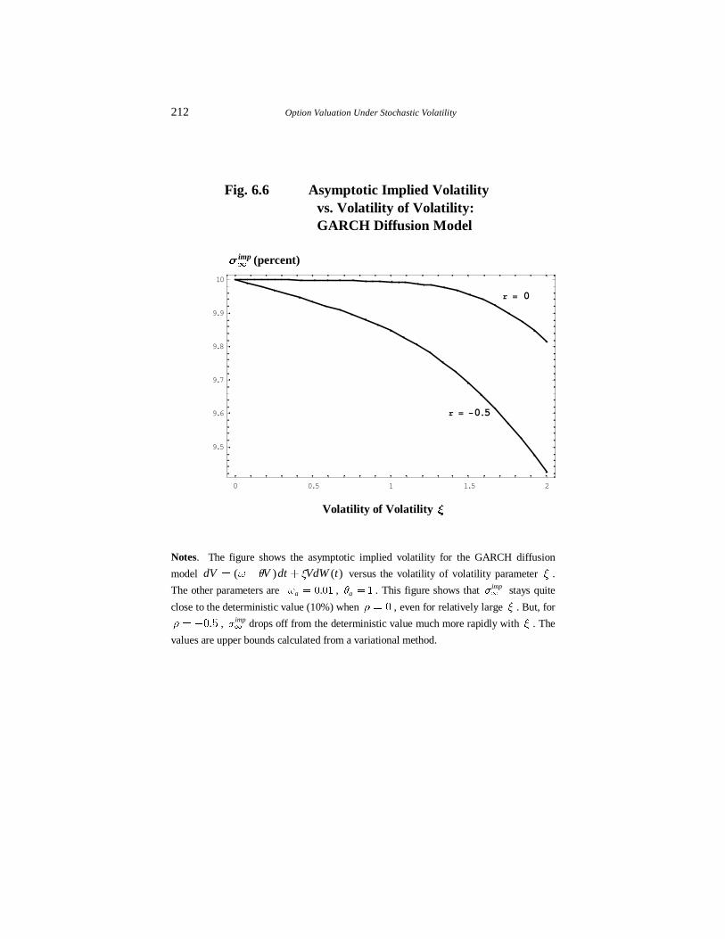
In Fig. 6.6 we plot impTd
versus the volatility of volatility Y for S � � and
.S ��� � . The other parameters are the same as Fig. 6.4. This figure showsthat impT
d stays quite close to the deterministic value when S � � , even for
relatively large Y . But, for .S ��� � , impTd
drops off from the deterministic
value much more rapidly with Y .
General processes. We now extend the variational principle to general risk-
adjusted processes of the form ( ) ( )dV b V dt a V dW� �� , with correlation ( )VS .This is the one subsection in this chapter where we assume a genuine risk-adjustment may be present. Under this general process, the evolution equation
for the fundamental transform has been given at (2.219).
204 Option Valuation Under Stochastic Volatility
It’s not useful to make exactly the same change of variable that we made for theGARCH diffusion. But we can make (2.2.19) similar by letting x V� and
ˆ ( , , ) ( , )H k V f xU U� . Then (2.2.19) becomes
(7.12) kf
fU
s��
s$ ,
where /( ) ( ) ( ) ( ) ( )kf f
f a x b x ik x a x x c k x fxx
Ss s
¯� � � � �¢ ± ss
�
� � ��
� �
�$ .
Just as in the GARCH diffusion, we assume that k iy� , where y is real and in
the interval y� �� � . Then, all of the coefficients in (7.12) are real-valued and
we can associate it with the auxiliary process:
(7.13) /( ) ( ) ( ) ( ) ( )dx b x ik x a x x dt a x dB tS ¯� � �¢ ±� �
� ,
where x� �d� , k iy� , y� �� � .
This can be written more compactly by defining the (real-valued) auxiliary driftcoefficient
(7.14) /( ) ( ) ( ) ( )k x b x ik x a x xC S� � � �� ,
so that (7.13) reads
(7.15) ( ) ( ) ( )kdx x dt a x dB tC� � , ( x� �d� , k iy� , y� �� � ).
The forward equation for the auxiliary process is
(7.16) < >( ) ( ) ( ) ( )kk k k k
pp a x p x x p x
xxC
U
s s s ¯� � �¢ ±s ss
c�
��
� �$ .
And there is a (time-independent) solution to kp �c�$ given by
(7.17) ( )
( ) exp( ) ( )
xk
ky
p x dya x a y
C ¯¡ °�¡ °¢ ±¨� �
�� ,
which is the analog of (7.4). Note that ( )kp x is a positive real number for all
( , )x k such that x� �d� , k iy� , ( y� �� � ). But ( )kp x is not necessarilyintegrable with respect to x.
The variational principle for the first eigenvalue then becomes
The Term Structure of Implied Volatility 205
(7.18) < > < >\ ^
< >( ) ( )
( ) ( ) ( ) ( ) ( )( ) min
( ) ( )
k
f x kk
p x a x f x c k x f x dxk
p x f x dxM
d
d
�
£ ²¦ ¦a �¦ ¦¦ ¦¦ ¦� ¤ »¦ ¦¦ ¦¦ ¦¦ ¦¥ ¼
¨
¨
� ���
��
�
�
$
.
The space ( )k$ of admissible functions consists of all real-valued functions that
satisfy, for k iy� , ( y� �� � ), the conditions:
(i) ,
lim ( ) ( ) ( ) ( )kx
a x p x f x f xl d
a ��
�
� ,
(ii) < >( ) ( )kp x f x dx �d¨ � , < >( ) ( )kp x x f x dx �d¨ � ,
< >( ) ( ) ( )kp x a x f x dxa �d¨�� .
Note that if a first eigenvalue exists for k iy� , ( y� �� � ), then it must bestrictly positive since every term in (7.18) is positive. So we really have a two-sided bound: M � � and M � the upper bound of (7.18).
General process (zero correlation). Let’s apply the general process variationalprinciple to the case S � � . In that case, the auxiliary process (7.14) is
independent of k and coincides with the risk-adjusted volatility process. So( )kp x is independent of k . Let’s assume that the risk-adjusted volatility process
has a long run stationary distribution ( )p V� and a finite first moment. Then
( ) ( )kp x p V� � , ( )p x is integrable and f � � is admissible. If we choosef � � for a trial function, then (7.18) implies that
(7.19) ( )
( ) ( )( )
V p V dVk c k
p V dVM
d
db
¨
¨�
�
�
�
,
The stationary point for the right-hand-side of (7.19) is, as we expect, at
/k i�� � , where ( / ) /c i �� � � . Moreover, since ( )p V� is integrable, let’snormalize the denominator to 1. Then, we have the bound:
(7.20) ( )impV V p V dVd
d b ¨�
� . ( )S � � �
Let’s check this result for the exactly solvable models. For example, for the 3/2
model, it’s easy to find the stationary distribution
/( ) exp /( )p V CV VR Y X Y� � ¯� �¢ ±�
� � ��� ,
206 Option Valuation Under Stochastic Volatility
where C is the normalization constant. For simplicity, assume ,X R � � . Then,(7.20) reads
impV R XRR Y
db
� �
�
� . (3/2 model)
This can be proven correct using the exact solution (5.3). It’s a tighter boundthan simply the deterministic limit ( Y �
�� ).
A second check is any model with a linear drift:( ) ( ) ( )dV V dt a V dW tX R� � � . In the case of linear drift models, we proved
in Appendix 5.1 (Example 1) that the long-run expected volatility is always
/X R , regardless of ( )a V . So for all linear drift models, (7.20) reads/impV X R
db , which was our previous result under the GARCH diffusion alone.
Finally, we could relax the assumption that ( )p V� have a first moment, since theinequality (7.20) also makes sense if the right-hand-side is �d .
An open issue. Suppose you’ve solved the PDE problem (2.2.19) for thefundamental transform ˆ ( , , )H k V U . Your solution turns out to be a regular
function in the complex k-plane in the strip Im kB C� � . Next, you letk iy� , where max[ , ] min[ , ]yB C� �� � . As U ld , you find thatˆ ( , , ) exp[ ( ) ] ( , )H k V k k VU M U Kx �� .
Separately, with k in the same interval, you’ve found ( )kM , the first eigenvaluesolution to ( )k u k uM�$ , ( )u k� $ , where ( )k$ is the class of admissible
functions defined in this section.
The open issue: is it always true that ( ) ( )k kM M� � ? In other words, we’ve really
just summarized the developments in Secs. 3 and 6, and are asking if theyalways lead to the same value for the asymptotic implied volatility. If they don’t,then the conditions that define the function space ( )k$ must be revised.
The Term Structure of Implied Volatility 207
8 A Differential Equation (DSolve) Method
In this section, we explain how to find the asymptotic implied volatility bysolving a differential equation9. Numerically, we do this with Mathematica’sDSolve function (actually NDSolve,to be precise)—hence the reference in
the section title.
The method is very fast and produces values in just a couple seconds of desktop
computer time. The variational method can be fast, too, with only a singleparameter being optimized. But if you want higher accuracy in the variationalmethod, you have to develop more complex trial functions, with more
parameters. As we indicated, this is something of an art. In contrast, the methodin this section, if you can set it up, can be made arbitrarily accurate just byadjusting function arguments.
A tradeoff is that the method in this section requires a certain asymptoticanalysis, which is explained below. The method works for the GARCH
diffusion, which is one of our main interests, because we can perform thatanalysis. For other models, you have to investigate.
Consider again the eigenvalue problem under GARCH diffusion process, givenat (6.1) and we repeat here for convenience
(8.1) / ( ) ( )d u duV V ik V c k V u k udVdV
Y X R SY M ¯� � � � � �¢ ±
�� � � ��
� �.
As before, consider k a purely imaginary parameter: k iy� and y is in theinterval y� �� � . So all of the coefficients in (8.1) are real numbers.
It makes the discussion simpler if we do a rescaling first, so multiply both sidesof (8.1) by / Y�� , and define new (real) parameters
X XY
��
�� , R R
Y�
�
�� ,
ikd
S
Y�
�� , c c
Y�
�
�� , z M
Y�
�
� .
Then (8.1) becomes
(8.2) /V u V dV u cV u z uX Raa a� � � � � �� � ��� �
� � .
9 The method in this section is adapted from a similar procedure in Aslanyanand Davies (1998)
208 Option Valuation Under Stochastic Volatility
We can find the first eigenvalue by the following procedure. First, forget thatz in (8.2) is related to an eigenvalue and just think of it a parameter that is fixed
at some real value, say 6. Then, it’s possible to develop asymptotic solutions for(8.2) both as V l � and V ld , which are singular points. Because (8.2) is asecond order equation, there are two such solutions in any regime. But the one
we report is the smaller one. Exactly how to do this is explained in Chapter 10;here we merely quote the results:
First, as V l � , we find that the “well-behaved” solution has the form:
(8.3) /( )zu a V O VX
¯x � �¡ °
¢ ±
� �
� ��
,
where a� is arbitrary. At the other extreme, as V ld , we find that the well-behaved solution has the form:
(8.4) exp
bu d V V b O
VV
B R
C� � ¯ ¯x � � �¡ °¢ ± ¡ °¢ ±
�
�� � ��
��
� ,
where ( )d R
BC
��
� �
�
� �
and ( ) ( )k k ikC I SY Y
�� �� � �� �� ��
and b� and b� are constants that play no role. In general, the method of thissection “works” whenever you can develop asymptotic solutions to theeigenvalue equation. This will be true in many models of interest. Next,
consider the function
(8.5) ( )
( )( )
u Vg V
u V
a� .
This function satisfies the first order (non-linear) differential equation, calledthe Riccati equation:
(8.6) /dgV V g V dV g cV z
dVX R� � � � � � �� � � � �
�� �
� �
Now pick a small value minV , a large value maxV and an arbitrary point a in
between: min maxV a V� � .
We can solve (8.6) in the interval minV V ab b by starting the solution at minV .
We start the solution by using (8.3), which implies that for small enough minV ,
(8.7) min( ) zg VX
x��
.
The Term Structure of Implied Volatility 209
Call this solution ( , )g V z� . Similarly, we can solve (8.6) in the interval
maxa V Vb b by using (8.4), which implies that for large enough maxV .
(8.8) maxmaxmax
( ) ( )( )
dg V
VV
C B R� � �x �
� � �
��
� �
.
Call this solution ( , )g V z� . Finally, define the function
(8.9) ( , ) ( , ) ( , ) ( , )
( ) ( , ) ( , )( , ) ( , )a
u a z u a z u a z u a zF z g a z g a z
u a z u a z
a a�� � � � � � �
� �
� �
.
Now for a general value of z, the solution which behaves like (8.3) as V l � , ifcontinued beyond the point V a� , will not behave like (8.4) as V ld .
There’s a second solution that grows much more rapidly than (8.4) as V ld ;call that one the “ill-behaved” solution (see Chapter 10 for its form). For anarbitrarily chosen value of z, if you start the solution with (8.3), and continue
that solution beyond the point V a� , you’ll get a mixture of the well-behavedsolution and the ill-behaved solution as V ld .
But, for /z z M Y� w �
� � , where M is the first eigenvalue, the solution( , )u V z� � , if it was continued beyond V a� , would be found proportional to
the well-behaved solution ( , )u V z� � , at least in the limit where minV l � and
maxV l�d . If ( , ) ( , )u V z mu V z�� � � � , with m a constant, then the numeratorin (8.9) vanishes and the denominator is proportional to ( , )u a z�
� , the square ofthe first eigenfunction.
If you increase z from zero, the first value at which ( )aF z vanishes must then bethe first (smallest) eigenvalue. Moreover, since we know the first eigenfunction
( , )u a z� is positive for all V, the denominator in (8.9) will not vanish when thenumerator does. To summarize, in the limit where minV l � and maxV l�d ,the first eigenvalue /zM Y� �
� � , where z� is the first (smallest) zero of
( )aF z on the real positive z-axis.
In Mathematica, the NDSolve function easily finds numerical solutions to
(8.6), creating ( )aF z . Then, FindRoot finds the zero z� of ( )aF z . All thishappens when the parameter k is fixed at a pure imaginary value in the vicinityof /k i� � . That is ( / ) ( )z kY M� �
� � and finally we use FindMinimum to
find the stationary value k� . The code is in the Appendix to this chapter.
210 Option Valuation Under Stochastic Volatility
A by-product of the calculation of M is that you then have available the fullfunction ( , )g V z� , which is defined over the entire range min maxV V Vb b by
min
max
( , ) ( , )
( , )
g V z V V ag V z
g V z a V V
£ b b¦¦� ¤¦ b b¦¥
� �
�
� �
Note that ( , )g V z� is continuous at V a� for any values of minV and
maxV because ( , ) ( , )g a z g a z�� � � � . Then, the first eigenfunction is given by thelimiting value, as the boundaries become exact, of
(8.10) ( ) exp ( , )V
au V g x z dx
¯� ¡ °
¡ °¢ ±¨ �
In Mathematica, the expression (8.10) evaluates extremely rapidly because( , )g x z� , being the result of a solution to a differential equation is an
“interpolating function” and such functions are rapidly integrated. We used(8.10) to produce the plots shown in Fig. 6.4. This code is also given in theAppendix.
The eigenvalues are independent of a in the limit that minV l � and
maxV l d . In practice, there’s a very weak dependence with finite endpoints.
Since a is a volatility value, a natural choice for the GARCH diffusion and theone we selected was /a X R� . A brief sensitivity analysis showed very littledifference in results if the value was 50% higher or lower.
Numerical results are shown in Table 6.3 below. As you can see, the values forthe asymptotic implied volatility are virtually indistinguishable from the
variational method results. The method is very straightforward, fast, and shouldbe easy to adapt to many models.
The Term Structure of Implied Volatility 211
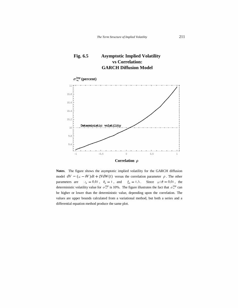
Fig. 6.5 Asymptotic Implied Volatility vs Correlation: GARCH Diffusion Model
impd
T (percent)
Correlation S
Notes. The figure shows the asymptotic implied volatility for the GARCH diffusion
model ( ) ( )dV V dt VdW tX R Y� � � versus the correlation parameter S . The other
parameters are .aX � � �� , aR � � , and .aY � � � . Since / .X R � � �� , the
deterministic volatility value for impTd is 10%. The figure illustrates the fact that impTd can
be higher or lower than the deterministic value, depending upon the correlation. The
values are upper bounds calculated from a variational method, but both a series and a
differential equation method produce the same plot.
-1 -0.5 0 0.5 1
9.6
9.8
10
10.2
10.4
10.6
10.8
11
Deterministic volatility
212 Option Valuation Under Stochastic Volatility
Fig. 6.6 Asymptotic Implied Volatility vs. Volatility of Volatility: GARCH Diffusion Model
impd
T (percent)
Volatility of Volatility Y
Notes. The figure shows the asymptotic implied volatility for the GARCH diffusion
model ( ) ( )dV V dt VdW tX R Y� � � versus the volatility of volatility parameter Y .
The other parameters are .aX � � �� , aR � � . This figure shows that impTd stays quite
close to the deterministic value (10%) when S � � , even for relatively large Y . But, for
.S ��� � , impTd drops off from the deterministic value much more rapidly with Y . The
values are upper bounds calculated from a variational method.
0 0.5 1 1.5 2
9.5
9.6
9.7
9.8
9.9
10
r = 0
r = -0.5
The Term Structure of Implied Volatility 213
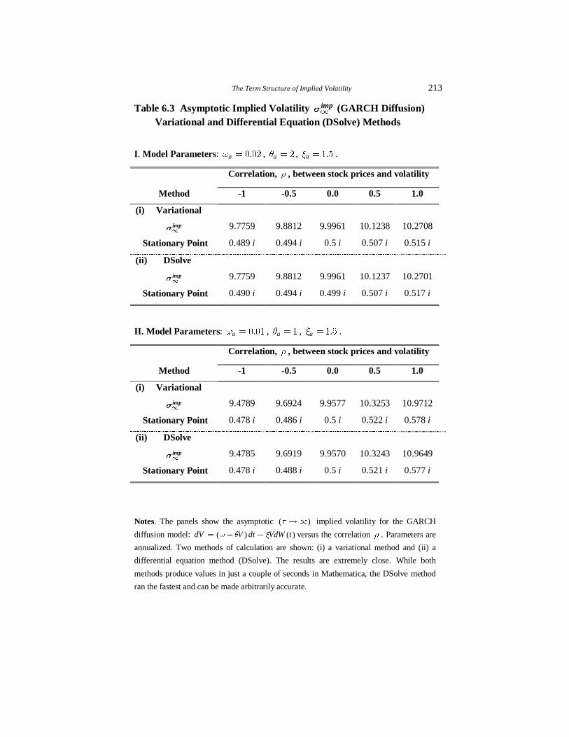
Table 6.3 Asymptotic Implied Volatility Td
imp (GARCH Diffusion) Variational and Differential Equation (DSolve) Methods
I. Model Parameters: .aX � � �� , aR � � , .aY � � � .
Correlation, S , between stock prices and volatility
Method -1 -0.5 0.0 0.5 1.0
(i) Variational
Td
imp 9.7759 9.8812 9.9961 10.1238 10.2708
Stationary Point 0.489 i 0.494 i 0.5 i 0.507 i 0.515 i
(ii) DSolve
Td
imp 9.7759 9.8812 9.9961 10.1237 10.2701
Stationary Point 0.490 i 0.494 i 0.499 i 0.507 i 0.517 i
II. Model Parameters: .aX � � �� , aR � � , .aY � � � .
Correlation, S , between stock prices and volatility
Method -1 -0.5 0.0 0.5 1.0
(i) Variational
Td
imp 9.4789 9.6924 9.9577 10.3253 10.9712
Stationary Point 0.478 i 0.486 i 0.5 i 0.522 i 0.578 i
(ii) DSolve
Td
imp 9.4785 9.6919 9.9570 10.3243 10.9649
Stationary Point 0.478 i 0.488 i 0.5 i 0.521 i 0.577 i
Notes. The panels show the asymptotic ( )U ld implied volatility for the GARCH
diffusion model: ( ) ( )dV V dt VdW tX R Y� � � versus the correlation S . Parameters are
annualized. Two methods of calculation are shown: (i) a variational method and (ii) a
differential equation method (DSolve). The results are extremely close. While both
methods produce values in just a couple of seconds in Mathematica, the DSolve method
ran the fastest and can be made arbitrarily accurate.