Option Valuation with Long-run and Short-runVolatility Components

Peter ChristoffersenMcGill University and CIRANO

Kris JacobsMcGill University and CIRANO

Yintian Wang∗

McGill University

October 12, 2004

Abstract

This paper presents a new model for the valuation of European options. In our model,the volatility of returns consists of two components. One of these components is along-run component, and it can be modeled as fully persistent. The other component isshort-run and has a zero mean. Our model can be viewed as an affine version of that inEngle and Lee (1999) allowing for easy valuation of European options. We investigatethe model empirically integrating returns and options data. The performance of themodel is spectacular when compared to a benchmark single-component volatility modelthat is well-established in the literature. The improvement in the model’s performanceis due to its richer dynamics which enable it to jointly model long-maturity and short-maturity options.

JEL Classification: G12

Keywords: option valuation; long-run component; short-run component; unobservedcomponents; persistence; GARCH; out-of-sample.

∗The first two authors are grateful for financial support from FQRSC, IFM2 and SSHRC. We would like tothank Tim Bollerslev, Frank Diebold, Bjorn Eraker, Steve Heston and Nour Meddahi for helpful discussion.Any remaining inadequacies are ours alone. Correspondence to: Kris Jacobs, Faculty of Management,McGill University, 1001 Sherbrooke Street West, Montreal, Canada H3A 1G5; Tel: (514) 398-4025; Fax:(514) 398-3876; E-mail: kris.jacobs@mcgill.ca.

1

1 Introduction

There is a consensus in the literature that combining time-variation in the conditional vari-ance of asset returns (Engle (1982), Bollerslev (1986)) with a leverage effect (Black (1976))constitutes a potential solution to well-known biases associated with the Black-Scholes (1973)model, such as the smile and the smirk. To model the smirk, these models generate higherprices for out-of-the-money put options as compared to the Black-Scholes formula. Equiv-alently, the models generate negative skewness in the distribution of asset returns. In thecontinuous-time option valuation literature, the Heston (1993) model addresses some of thesebiases. This model contains a leverage effect as well as stochastic volatility.1 In the discrete-time literature, the NGARCH(1,1) option valuation model proposed by Duan (1995) containstime-variation in conditional variance as well as a leverage effect. The model by Heston andNandi (2000) is closely related to Duan’s model.Many existing empirical studies have confirmed the importance of time-varying volatility

and the leverage effect in continuous-time and discrete-time setups.2 However, it has be-come clear that while these models help explain the biases of the Black-Scholes model in aqualitative sense, they come up short in a quantitative sense. Using parameters estimatedfrom returns or options data, these models reduce the biases of the Black-Scholes model, butthe magnitude of the effects is insufficient to completely resolve the biases. The resultingpricing errors have the same sign as the Black-Scholes pricing errors, but are smaller in mag-nitude. We therefore need models that possess the same qualitative features as the modelsin Heston (1993) and Duan (1995), but that contain stronger quantitative effects. Thesemodels need to generate more flexible skewness and volatility of volatility dynamics in orderto fit observed option prices.One interesting approach in this respect is the inclusion of jump processes. In most

existing studies, jumps are added to models that already contain time-variation in the con-ditional variance as well as a leverage effect. The empirical findings in this literature havebeen mixed. In general jumps in returns and volatility improve option valuation when para-meters are estimated using historical time series of returns, but usually not when parametersare estimated using the cross-section of option prices.3

This paper takes a different approach. We attempt to remedy the remaining optionbiases by modeling richer volatility dynamics.4 It has been observed using a variety of

1The importance of stochastic volatility is also studied in Hull and White (1987), Melino and Turnbull(1990), Scott (1987) and Wiggins (1987).

2See for example Amin and Ng (1993), Bakshi, Cao and Chen (1997), Bates (1996, 2000), Benzoni (1998),Bollerslev and Mikkelsen (1999), Chernov and Ghysels (2000), Duan, Ritchken and Sun (2004), Engle andMustafa (1992), Eraker (2004), Heston and Nandi (2000), Jones (2003), Nandi (1998) and Pan (2003).

3See for example Bakshi, Cao and Chen (1997), Eraker, Johannes and Polson (2003), Eraker (2004) andPan (2002).

4Adding jumps to the new volatility specification may of course improve the model further.

2

diagnostics that it is difficult to fit the autocorrelation function of return volatility using abenchmark model such as a GARCH(1,1). Even though the comparison between discreteand continuous-time models is sometimes tenuous (see Corradi (2000)), similar remarks applyto stochastic volatility models such as Heston (1993). The main problem is that volatilityautocorrelations are too high at longer lags to be explained by a GARCH(1,1), unless theprocess is extremely persistent. This extreme persistence may impact negatively on otheraspects of option valuation, such as the valuation of short-maturity options.In fact, it has been observed in the literature that volatility may be better modeled using

a fractionally integrated process, rather than a stationary GARCH process.5 Andersen,Bollerslev, Diebold and Labys (2003) confirm this finding using realized volatility. Bollerslevand Mikkelsen (1996, 1999) and Comte, Coutin and Renault and (2001) investigate anddiscuss some of the implications of long memory for option valuation. Using fractionalintegration models for option valuation is cumbersome. Optimization is very time-intensiveand a number of ad-hoc choices have to be made regarding implementation. This paperaddresses the same issues using a different type of model that is easier to implement andcaptures the stylized facts addressed by long-memory models at horizons relevant for optionvaluation. The model builds on Heston and Nandi (2000 and Engle and Lee (1999). In ourmodel, the volatility of returns consists of two components. One of these components is along-run component, and it can be modeled as (fully) persistent. The other component isshort-run and mean zero. The model is able to generate autocorrelation functions that arericher than those of a GARCH(1,1) model while using just a few additional parameters. Weillustrate how this impacts on option valuation by studying the term structure of volatility.Unobserved component or factor models are very popular in the finance literature. See

Fama and French (1988), Poterba and Summers (1988) and Summers (1986) for applicationsto stock prices. In the option pricing literature, Bates (2000) and Taylor and Xu (1994)investigate two-factor stochastic volatility models. Eraker (2004) suggests the usefulness ofour approach based on stylized facts emanating from his empirical study. Alizadeh, Brandtand Diebold (2002) uncover two factors in stochastic volatility models of exchange ratesusing range-based estimation. Unobserved component models are also very popular in theterm structure literature, although in this literature the models are more commonly referredto as multifactor models.6 There are very interesting parallels between our approach andresults and stylized facts in the term structure literature. In the term structure literatureit is customary to model short-run fluctuations around a time-varying long-run mean of theshort rate. In our framework we model short-run fluctuations around time-varying long-runvolatility.Dynamic factor and component models can be implemented in continuous or discrete

5See Baillie, Bollerslev and Mikkelsen (1996) and Chernov, Gallant, Ghysels and Tauchen (2003).6See for example Dai and Singleton (2000), Duffee (1999), Duffie and Singleton (1999) and Pearson and

Sun (1994).

3

time. We choose a discrete-time approach because of the ease of implementation. Inparticular, our model is related to the GARCH class of processes and volatility filtering andforecasting are relatively straightforward, which is critically important for option valuation.An additional advantage of our model is parsimony: the most general model we investigatehas seven parameters. The models with jumps in returns and volatility discussed aboveare much more heavily parameterized. We speculate that parsimony may help our model’sout-of-sample performance.We investigate the model empirically using an approach integrating returns and options

data. We study two models: one where the long-run component is constrained to be fullypersistent and one where it is not. We refer to these models as the persistent componentmodel and the component model respectively. When persistence of the long-run componentis freely estimated, it is very close to one. The performance of the component model isspectacular when compared with a benchmark GARCH(1,1) model. The improvement inthe model’s performance is due to its richer dynamics, which enable it to jointly modellong-maturity and short-maturity options. Our out-of-sample results strongly suggest thatthese richer dynamics are not simply due to spurious in-sample overfitting. The persistentcomponent model performs better than the benchmark GARCH(1,1) model, but it is inferiorto the component model both in- and out-of-sample. We also provide a detailed study ofthe term structure of volatilities for our proposed models and the benchmark model.The paper proceeds as follows. Section 2 introduces the model. Section 3 discusses the

volatility term structure and Section 4 discusses option valuation. Section 5 discusses theempirical results, and Section 6 concludes.

2 Return Dynamics with Volatility Components

In this section we first present the Heston-Nandi GARCH(1,1) model which will serve asthe benchmark model throughout the paper. We then construct the component model as anatural extension of a rearranged version of the GARCH(1,1) model. Finally the persistentcomponent model is presented as a special case of the component model.

2.1 The Heston and Nandi GARCH(1,1) Model

Heston and Nandi (2000) propose a class of GARCH models that allow for a closed-formsolution for the price of a European call option. They present an empirical analysis of theGARCH(1,1) version of this model, which is given by

ln(St+1) = ln(St) + r + λht+1 +pht+1zt+1 (1)

ht+1 = w + b1ht + a1(zt − c1pht)

2

4

where St+1 denotes the underlying asset price, r the risk free rate, λ the price of risk andht+1 the daily variance on day t+ 1 which is known at the end of day t. The zt+1 shock isassumed to be i.i.d. N(0, 1). The Heston-Nandi model captures time variation in the con-ditional variance as in Engle (1982) and Bollerslev (1986),7 and the parameter c1 capturesthe leverage effect. The leverage effect captures the negative relationship between shocksto returns and volatility (Black (1976)), which results in a negatively skewed distribution ofreturns. Its importance for option valuation has been emphasized among others by Ben-zoni (1998), Chernov and Ghysels (2000), Christoffersen and Jacobs (2004), Eraker (2004),Eraker, Johannes and Polson (2003), Heston (1993), Heston and Nandi (2000) and Nandi(1998). It must be noted at this point that the GARCH(1,1) dynamic in (1) is slightlydifferent from the more conventional NGARCH model used by Engle and Ng (1993) andHentschel (1995), which is used for option valuation in Duan (1995). The reason is that thedynamic in (1) is engineered to yield a closed-form solution for option valuation, whereas aclosed-form solution does not obtain for the more conventional GARCH dynamic. Hsieh andRitchken (2000) provide evidence that the more traditional GARCH model may actuallyslightly dominate the fit of (1). Our main point can be demonstrated using either dynamic.Because of the convenience of the closed-form solution provided by dynamics such as (1),we use this as a benchmark in our empirical analysis and we model the richer componentstructure within the Heston-Nandi framework.To better appreciate the workings of the component models presented below, note that

by using the expression for the unconditional variance

E [ht+1] ≡ σ2 =w + a1

1− b1 − a1c21

the variance process can now be rewritten as

ht+1 = σ2 + b1¡ht − σ2

¢+ a1

³(zt − c1

pht)

2 − (1 + c21σ2)´

(2)

2.2 Building a Component Volatility Model

The expression for the GARCH(1,1) variance process in (2) highlights the role of the para-meter σ2 as the constant unconditional mean of the conditional variance process. A naturalgeneralization is then to specify σ2 as time-varying. Denoting this time-varying componentby qt+1, the expression for the variance in (2) can be generalized to

ht+1 = qt+1 + β (ht − qt) + α³(zt − γ1

pht)

2 − (1 + γ21qt)´

(3)

This model is similar in spirit to the component model of Engle and Lee (1999). Thedifference between our model and Engle and Lee (1999) is that the functional form of the

7For a leading finance application of GARCH see French, Schwert and Stambaugh (1987).

5

GARCH dynamic (3) allows for a closed-form solution for European option prices. This issimilar to the difference between the Heston-Nandi (2000) GARCH(1,1) dynamic and themore traditional NGARCH(1,1) dynamic discussed in the previous subsection. In specifi-cation (3), the conditional volatility ht+1 can most usefully be thought of as consisting oftwo components. Following Engle and Lee (1999), we refer to the component qt+1 as thelong-run component, and to ht+1 − qt+1 as the short-run component. We will discuss thisterminology in some more detail below. Note that by construction the unconditional meanof the short-run component ht+1 − qt+1 is zero.The model can also be written as

ht+1 = qt+1 + (αγ21 + β) (ht − qt) + α

³(zt − γ1

pht)

2 − (1 + γ21ht)´

= qt+1 + β̃ (ht − qt) + α³(zt − γ1

pht)

2 − (1 + γ21ht)´

(4)

where β̃ = αγ21 + β. This representation is useful because we can think of

v1,t ≡³zt − γ1

pht´2− (1 + γ21ht) (5)

=¡z2t − 1

¢− 2γ1phtzt

as a mean-zero innovation.The model is completed by specifying the functional form of the long-run volatility com-

ponent. In a first step, we assume that qt+1 follows the process

qt+1 = ω + ρqt + ϕ³¡z2t − 1

¢− 2γ2phtzt´

(6)

Note that we can therefore write the component volatility model as

ht+1 = qt+1 + β̃ (ht − qt) + αv1,t (7)

qt+1 = ω + ρqt + ϕv2,t

withvi,t =

¡z2t − 1

¢− 2γiphtzt, for i = 1, 2. (8)

and Et−1 [vi,t] = 0, i = 1, 2. Also note that the model contains seven parameters: α, β̃, γ1,γ2, ω, ρ and ϕ in addition to the price of risk, λ.

2.3 A Fully Persistent Special Case

In our empirical work, we also investigate a special case of the model in (7). Notice that in(7) the long-run component of volatility will be a mean reverting process for ρ < 1. We also

6

estimate a version of the model which imposes ρ = 1. The resulting process is

ht+1 = qt+1 + β̃ (ht − qt) + αv1,t (9)

qt+1 = ω + qt + ϕv2,t

and vi,t, i = 1, 2 as in (8). The model now contains six parameters: α, β̃, γ1, γ2, ω and ϕ inaddition to the price of risk, λ.In this case the process for long-run volatility contains a unit root and shocks to the long-

run volatility never die out: they have a “permanent” effect. Recall that following Engleand Lee (1999) in (7) we refer to qt+1 as the long-run component and to ht+1 − qt+1 as theshort-run component. In the special case (9) we can also refer to qt+1 as the “permanent”component, because innovations to qt+1 are truly “permanent” and do not die out. Itis then customary to refer to ht+1 − qt+1 as the “transitory” component, which reverts tozero. It is in fact this permanent-effects version of the model that is most closely related tomodels which have been studied more extensively in the finance and economics literature,rather than the more general model in (7).8 We will refer to this model as the persistentcomponent model.It is clear that (9) is nested by (7). It is therefore to be expected that the in-sample

fit of (7) is superior. However, out-of-sample this may not necessarily be the case. It isoften the case that more parsimonious models perform better out-of-sample if the restrictionimposed by the model is a sufficiently adequate representation of reality. The persistentcomponent model may also be better able to capture structural breaks in volatility out-of-sample, because a unit root in the process allows it to adjust to a structural break, whichnot possible for a mean-reverting process. It will therefore be of interest to verify how closeρ is to one when estimating the more general model (7).

3 Variance Term Structures

To intuitively understand the shortcomings of existing models such as the GARCH(1,1)model in (1) and the improvements provided by our model (7), it is instructive to graphicallyillustrate the workings of both models in a dimension that critically affects their performance.In this section we graphically illustrate the variance term structures and some other relatedproperties of the models that are key for option valuation.

8See Fama and French (1988), Poterba and Summers (1988) and Summers (1986) for applications to stockprices. See Beveridge and Nelson (1981) for an application to macroeconomics.

7

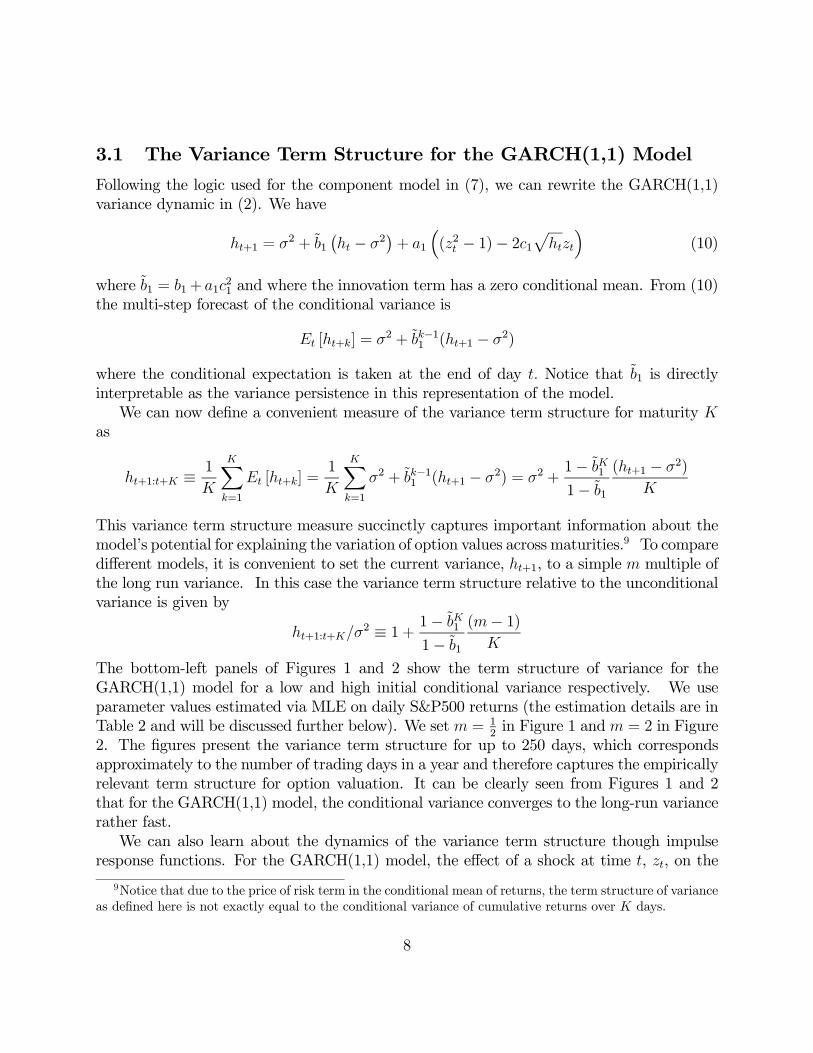
3.1 The Variance Term Structure for the GARCH(1,1) Model

Following the logic used for the component model in (7), we can rewrite the GARCH(1,1)variance dynamic in (2). We have

ht+1 = σ2 + b̃1¡ht − σ2

¢+ a1

³(z2t − 1)− 2c1

phtzt

´(10)

where b̃1 = b1+ a1c21 and where the innovation term has a zero conditional mean. From (10)

the multi-step forecast of the conditional variance is

Et [ht+k] = σ2 + b̃k−11 (ht+1 − σ2)

where the conditional expectation is taken at the end of day t. Notice that b̃1 is directlyinterpretable as the variance persistence in this representation of the model.We can now define a convenient measure of the variance term structure for maturity K

as

ht+1:t+K ≡ 1

K

KXk=1

Et [ht+k] =1

K

KXk=1

σ2 + b̃k−11 (ht+1 − σ2) = σ2 +1− b̃K11− b̃1

(ht+1 − σ2)

K

This variance term structure measure succinctly captures important information about themodel’s potential for explaining the variation of option values across maturities.9 To comparedifferent models, it is convenient to set the current variance, ht+1, to a simple m multiple ofthe long run variance. In this case the variance term structure relative to the unconditionalvariance is given by

ht+1:t+K/σ2 ≡ 1 + 1− b̃K1

1− b̃1

(m− 1)K

The bottom-left panels of Figures 1 and 2 show the term structure of variance for theGARCH(1,1) model for a low and high initial conditional variance respectively. We useparameter values estimated via MLE on daily S&P500 returns (the estimation details are inTable 2 and will be discussed further below). We set m = 1

2in Figure 1 and m = 2 in Figure

2. The figures present the variance term structure for up to 250 days, which correspondsapproximately to the number of trading days in a year and therefore captures the empiricallyrelevant term structure for option valuation. It can be clearly seen from Figures 1 and 2that for the GARCH(1,1) model, the conditional variance converges to the long-run variancerather fast.We can also learn about the dynamics of the variance term structure though impulse

response functions. For the GARCH(1,1) model, the effect of a shock at time t, zt, on the

9Notice that due to the price of risk term in the conditional mean of returns, the term structure of varianceas defined here is not exactly equal to the conditional variance of cumulative returns over K days.

8

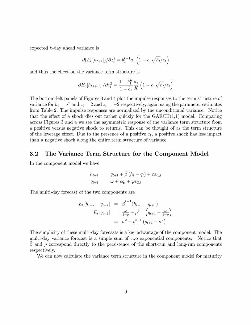
expected k-day ahead variance is

∂(Et [ht+k])/∂z2t = b̃k−11 a1

³1− c1

pht/zt

´and thus the effect on the variance term structure is

∂Et [ht:t+K ] /∂z2t =

1− b̃K11− b̃1

a1K

³1− c1

pht/zt

´The bottom-left panels of Figures 3 and 4 plot the impulse responses to the term structure ofvariance for ht = σ2 and zt = 2 and zt = −2 respectively, again using the parameter estimatesfrom Table 2. The impulse responses are normalized by the unconditional variance. Noticethat the effect of a shock dies out rather quickly for the GARCH(1,1) model. Comparingacross Figures 3 and 4 we see the asymmetric response of the variance term structure froma positive versus negative shock to returns. This can be thought of as the term structureof the leverage effect. Due to the presence of a positive c1, a positive shock has less impactthan a negative shock along the entire term structure of variance.

3.2 The Variance Term Structure for the Component Model

In the component model we have

ht+1 = qt+1 + β̃ (ht − qt) + αv1,t

qt+1 = ω + ρqt + ϕv2,t

The multi-day forecast of the two components are

Et [ht+k − qt+k] = β̃k−1(ht+1 − qt+1)

Et [qt+k] =ω1−ρ + ρk−1

³qt+1 − ω

1−ρ´

≡ σ2 + ρk−1¡qt+1 − σ2

¢The simplicity of these multi-day forecasts is a key advantage of the component model. Themulti-day variance forecast is a simple sum of two exponential components. Notice thatβ̃ and ρ correspond directly to the persistence of the short-run and long-run componentsrespectively.We can now calculate the variance term structure in the component model for maturity

9

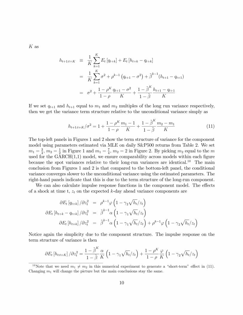
K as

ht+1:t+K ≡ 1

K

KXk=1

Et [qt+k] +Et [ht+k − qt+k]

=1

K

KXk=1

σ2 + ρk−1¡qt+1 − σ2

¢+ β̃

k−1(ht+1 − qt+1)

= σ2 +1− ρK

1− ρ

qt+1 − σ2

K+1− β̃

K

1− β̃

ht+1 − qt+1K

If we set qt+1 and ht+1 equal to m1 and m2 multiples of the long run variance respectively,then we get the variance term structure relative to the unconditional variance simply as

ht+1:t+K/σ2 = 1 +

1− ρK

1− ρ

m1 − 1K

+1− β̃

K

1− β̃

m2 −m1

K(11)

The top-left panels in Figures 1 and 2 show the term structure of variance for the componentmodel using parameters estimated via MLE on daily S&P500 returns from Table 2. We setm1 =

34, m2 =

12in Figure 1 and m1 =

74, m2 = 2 in Figure 2. By picking m2 equal to the m

used for the GARCH(1,1) model, we ensure comparability across models within each figurebecause the spot variances relative to their long-run variances are identical.10 The mainconclusion from Figures 1 and 2 is that compared to the bottom-left panel, the conditionalvariance converges slower to the unconditional variance using the estimated parameters. Theright-hand panels indicate that this is due to the term structure of the long-run component.We can also calculate impulse response functions in the component model. The effects

of a shock at time t, zt on the expected k-day ahead variance components are

∂Et [qt+k] /∂z2t = ρk−1ϕ

³1− γ2

pht/zt

´∂Et [ht+k − qt+k] /∂z

2t = β̃

k−1α³1− γ1

pht/zt

´∂Et [ht+k] /∂z

2t = β̃

k−1α³1− γ1

pht/zt

´+ ρk−1ϕ

³1− γ2

pht/zt

´Notice again the simplicity due to the component structure. The impulse response on theterm structure of variance is then

∂Et [ht:t+K] /∂z2t =

1− β̃K

1− β̃

α

K

³1− γ1

pht/zt

´+1− ρK

1− ρ

ϕ

K

³1− γ2

pht/zt

´10Note that we need m1 6= m2 in this numerical experiment to generate a “short-term” effect in (11).

Changing m1 will change the picture but the main conclusions stay the same.

10

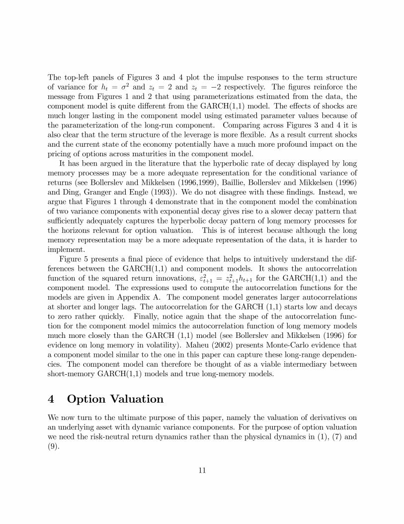
The top-left panels of Figures 3 and 4 plot the impulse responses to the term structureof variance for ht = σ2 and zt = 2 and zt = −2 respectively. The figures reinforce themessage from Figures 1 and 2 that using parameterizations estimated from the data, thecomponent model is quite different from the GARCH(1,1) model. The effects of shocks aremuch longer lasting in the component model using estimated parameter values because ofthe parameterization of the long-run component. Comparing across Figures 3 and 4 it isalso clear that the term structure of the leverage is more flexible. As a result current shocksand the current state of the economy potentially have a much more profound impact on thepricing of options across maturities in the component model.It has been argued in the literature that the hyperbolic rate of decay displayed by long

memory processes may be a more adequate representation for the conditional variance ofreturns (see Bollerslev and Mikkelsen (1996,1999), Baillie, Bollerslev and Mikkelsen (1996)and Ding, Granger and Engle (1993)). We do not disagree with these findings. Instead, weargue that Figures 1 through 4 demonstrate that in the component model the combinationof two variance components with exponential decay gives rise to a slower decay pattern thatsufficiently adequately captures the hyperbolic decay pattern of long memory processes forthe horizons relevant for option valuation. This is of interest because although the longmemory representation may be a more adequate representation of the data, it is harder toimplement.Figure 5 presents a final piece of evidence that helps to intuitively understand the dif-

ferences between the GARCH(1,1) and component models. It shows the autocorrelationfunction of the squared return innovations, ε2t+1 = z2t+1ht+1 for the GARCH(1,1) and thecomponent model. The expressions used to compute the autocorrelation functions for themodels are given in Appendix A. The component model generates larger autocorrelationsat shorter and longer lags. The autocorrelation for the GARCH (1,1) starts low and decaysto zero rather quickly. Finally, notice again that the shape of the autocorrelation func-tion for the component model mimics the autocorrelation function of long memory modelsmuch more closely than the GARCH (1,1) model (see Bollerslev and Mikkelsen (1996) forevidence on long memory in volatility). Maheu (2002) presents Monte-Carlo evidence thata component model similar to the one in this paper can capture these long-range dependen-cies. The component model can therefore be thought of as a viable intermediary betweenshort-memory GARCH(1,1) models and true long-memory models.

4 Option Valuation

We now turn to the ultimate purpose of this paper, namely the valuation of derivatives onan underlying asset with dynamic variance components. For the purpose of option valuationwe need the risk-neutral return dynamics rather than the physical dynamics in (1), (7) and(9).

11

4.1 The Risk-Neutral GARCH(1,1) Dynamic

The risk-neutral dynamics for the GARCH(1,1) model are given in Heston and Nandi(2000)11 as

ln(St+1) = ln(St) + r − 12ht+1 +

pht+1z

∗t+1 (12)

ht+1 = w + b1ht + a1(z∗t − c∗1

pht)

2

with c∗1 = c1 + λ + 0.5 and z∗t ∼ N(0, 1). For the component volatility models, the mostconvenient way to express the risk-neutral dynamics is to use the following mapping withthe GARCH(2,2) model.

4.2 The GARCH(2,2) Mapping

In order to construct the mapping from a component model to a GARCH(2,2) model notethat qt+1 in (6) can be written as

qt+1 =ω + ϕ

¡(z2t − 1)− 2γ2

√htzt

¢1− ρL

where L denotes the lag operator. Substituting this expression and its lagged version intothe expression for ht+1 in (4), it becomes clear that we can write the conditional variance inthe component model as a GARCH (2, 2) process.

ln(St+1) = ln(St) + r + λht+1 +pht+1zt+1 (13)

ht+1 = w + b1ht + b2ht−1 + a1

³zt − c1

pht

´2+ a2

³zt−1 − c2

pht−1

´2where

a1 = α+ ϕ (14)

a2 = −(ρα+ β̃ϕ)

b1 =³ρ+ β̃

´− (αγ1 + ϕγ2)

2

a1

b2 = −(ραγ1 + β̃ϕγ2)2

a2− ρβ̃

c1 =γ1α+ γ2ϕ

a1

c2 = −ργ1α+ ϕγ2β̃

a2w = (ω − ϕ) (1− β̃)− α (1− ρ)

11For the underlying theory on risk neutral distributions in discrete time option valuation see Rubinstein(1976), Brennan (1979), Amin and Ng (1993), Duan (1995), Camara (2003), and Schroeder (2004).

12

The relationship between the model in (13) and the model in (7) deserves more comment.Equation (14) shows that the component model can be viewed as a GARCH(2,2) model withnonlinear parameter restrictions. These restrictions yield the component structure whichenables interpretation of the model as having a potentially persistent long-run componentand a rapidly mean-reverting short-run component. We implement the model and presentthe empirical results in terms of the component parameters rather than the GARCH(2,2) pa-rameters. This interpretation of the results is very helpful when thinking about the varianceterm structure implications of the model, as Figures 1-4 above illustrate. The componentstructure allows for simple term structure formulas which in the general GARCH(2,2) modelare much more cumbersome and harder to interpret. Due to its natural extension of theGARCH(1,1) model, the component model is also useful for implementation when sensibleparameter starting values must be chosen for estimation. In contrast, it is quite difficult tocome up with sensible starting values for estimating a GARCH(2,2) process.The restrictions in (14) allow us to obtain the GARCH(2,2) parameters given the com-

ponents estimates. A natural question is if we can obtain the component parameters givenGARCH(2,2) estimates. In Appendix B we invert the mapping in (14) to get the componentmodel parameters as functions of the GARCH(2,2) parameters. The mapping illustratesmore advantages from implementing the component model as opposed to a GARCH(2,2)model: the stationarity requirements in the GARCH(2,2) model are quite complicated butin the component model we simply need β̃ < 1 and ρ < 1. The upshot is that the compo-nent model is much easier to implement from the point of view of finding reasonable startingvalues and enforcing stationarity in estimation.The mapping between the component model and the GARCH(2,2) model is most useful

for the purpose of option valuation. For option valuation, we need the risk-neutral dynamic.For the GARCH(2,2) model in (13), the risk-neutral representation is

ln(St+1) = ln(St) + r − 12ht+1 +

pht+1z

∗t+1 (15)

ht+1 = w + b1ht + b2ht−1 + a1³z∗t − c∗1

pht´2+ a2

³z∗t−1 − c∗2

pht−1

´2where c∗i = ci + λ+ 0.5, i = 1, 2 and z∗t ∼ N(0, 1).

4.3 The Option Valuation Formula

Given the risk-neutral dynamics, option valuation is relatively straightforward. We use theresult of Heston and Nandi (2000) that at time t, a European call option with strike price

13

K that expires at time T is worth

Call Price = e−r(T−t)E∗t [Max(ST −K, 0)] (16)

=1

2St +

e−r(T−t)

π

Z ∞

0

Re

·K−iφf∗(t, T ; iφ+ 1)

iφ

¸dφ

−Ke−r(T−t)µ1

2+1

π

Z ∞

0

Re

·K−iφf∗(t, T ; iφ)

iφ

¸dφ

¶where f∗(t, T ; iφ) is the conditional characteristic function of the logarithm of the spot priceunder the risk neutral measure. For the return dynamics in this paper, we can characterizethe generating function of the stock price with a set of difference equations. We apply thetechniques in Heston and Nandi (2000) to get for the GARCH(2,2) representation of themodel in (15):

f(t, T ;φ) = Sφt exp

³At +B1tht+1 +B2tht + Ct(zt − c2

pht)

2´

with coefficients

At = At+1 + φr +B1t+1w − 12ln (1− 2a1B1t+1 − 2Ct+1)

B1t = φ(−0.5) + 1/2φ2 + 2 (B1t+1a1c1 + Ct+1c2) (B1t+1a1c1 + Ct+1c2 − φ)

1− 2B1t+1a1 − 2Ct+1

+¡B1t+1a1c

21 + Ct+1c

22

¢+ b1B1t+1 +B2t+1

B2t = b2B1t+1

Ct = a2B1t+1

where At, B1t, B2t, and Ct implicitly are functions of T and φ. This system of differenceequations can be solved backwards using the terminal condition

AT = B1T = B2T = CT = 0.

Note that this result for the GARCH(2,2) model is different from the one listed in Ap-pendix A of Heston and Nandi (2000), which contains some typos. We present the derivationfor the GARCH(2,2) model in Appendix C and also present a correction of the general resultin the GARCH(p,q) case.12

12The accuracy of our results was verified by comparing the closed-form expressions with numerical results.The empirical results in Heston and Nandi (2000) are for the GARCH(1,1) case and are not affected by thisdiscrepancy for higher-order models. Our implementation of the pricing for the GARCH(1,1) case thus usesthe expressions in Heston and Nandi (2000). Finally, for completeness we also report the moment generatingfunction explicitly in terms of the component model in Appendix D, even though we do not use this resultin the implementation.

14

5 Empirical Results

This section presents the empirical results. We first discuss the data, followed by an empiricalevaluation of the model estimated under the physical measure using a historical series of stockreturns. Subsequently we present estimation results obtained by estimating the risk-neutralversion of the model using options data.

5.1 Data

We conduct our empirical analysis using six years of data on S&P 500 call options, for theperiod 1990-1995. We apply standard filters to the data following Bakshi, Cao and Chen(1997). We only use Wednesday options data. Wednesday is the day of the week least likelyto be a holiday. It is also less likely than other days such as Monday and Friday to beaffected by day-of-the-week effects. For those weeks where Wednesday is a holiday, we usethe next trading day. The decision to pick one day every week is to some extent motivatedby computational constraints. The optimization problems are fairly time-intensive, andlimiting the number of options reduces the computational burden. Using only Wednesdaydata allows us to study a fairly long time-series, which is useful considering the highlypersistent volatility processes. An additional motivation for only using Wednesday data isthat following the work of Dumas, Fleming and Whaley (1998), several studies have usedthis setup (see for instance Heston and Nandi (2000)).We perform a number of in-sample and out-of-sample experiments using the options data.

We first estimate the model parameters using the 1990-1992 data and subsequently test themodel out-of-sample using the 1993 data. We also estimate the model parameters usingthe 1992-1994 data and subsequently test the model out-of-sample using the 1995 data. Forboth estimation exercises we use a volatility updating rule for the 500 days predating theWednesday used in the estimation exercise. This volatility updating rule is initialized atthe model’s unconditional variance. We also perform an extensive empirical analysis usingreturn data. Ideally we would like to use the same sample periods for these estimationexercises, but it is well-known that it is difficult to estimate GARCH parameters preciselyusing relatively short samples on returns. We therefore use a long sample of returns (1963-1995) on the S&P 500.Table 1 presents descriptive statistics for the options data for 1990-1995 by moneyness

and maturity. Panels A and B indicate that the data are standard. We can clearly observethe volatility smirk from Panel C and it is clear that the slope of the smirk differs acrossmaturities. Descriptive statistics for different sub-periods (not reported here) demonstratethat the slope also changes across time, but that the smirk is present throughout the sample.The top panel of Figure 6 gives some indication of the pattern of implied volatility over time.For the 312 days of options data used in the empirical analysis, we present the average impliedvolatility of the options on that day. It is evident from Figure 6 that there is substantial

15

clustering in implied volatilities. It can also be seen that volatility is higher in the earlypart of the sample. The bottom panel of Figure 6 presents a time series for the 30-dayat-the-money volatility (VIX) index from the CBOE for our sample period. A comparisonwith the top panel clearly indicates that the options data in our sample are representativeof market conditions, although the time series based on our sample is of course a bit morenoisy due to the presence of options with different moneyness and maturities.

5.2 Empirical Results using Returns Data

Table 2 presents estimation results obtained using returns data for 1963-1995 for the physicalmodel dynamics. We present results for three models: the GARCH(1,1) model (1), thecomponent model (7) and the persistent component model (9). Almost all parameters areestimated significantly different from zero at conventional significance levels.13 In terms offit, the log likelihood values indicate that the fit of the component model is much better thanthat of the persistent component model, which in turn fits much better than the GARCH(1,1)model.The improvement in fit for the component GARCH model over the persistent compo-

nent GARCH model is perhaps somewhat surprising when inspecting the persistence of thecomponent GARCH model. The persistence is equal to 0.996. It therefore would appearthat equating this persistence to 1, as is done in the persistent component model, is aninteresting hypothesis, but apparently modeling these small differences from one is impor-tant. It must of course be noted that the picture is more complex: while the persistenceof the long-run component (ρ) is 0.990 for the component model as opposed to 1 for thepersistent component model, the persistence of the short-run component (β̃) is 0.644 versus0.764 and this may account for the differences in performance. Note that the persistenceof the GARCH(1,1) model is estimated at 0.955, which is consistent with earlier literature.It is slightly lower than the estimate in Christoffersen, Heston and Jacobs (2004) and a bithigher than the average of the estimates in Heston and Nandi (2000).The ability of the models to generate richer patterns for the conditional versions of

leverage and volatility of volatility is critical. For option valuation, the conditional versionsof these quantities and their variation through time are just as important as the unconditionalversions. The conditional versions of leverage and volatility of volatility are computed asfollows. For the GARCH(1,1) model the conditional variance of variance is

V art(ht+2) = Et [ht+2 − Et [ht+2]]2 (17)

= 2a21 + 4a21c21ht+1

13The standard errors are computed using the outer product of the gradient at the optimal parametervalues.

16

and the leverage effect can be defined as

Covt(ln (St+1) , ht+2) = Et [(ln (St+1)−Et [ln (St+1)]) (ht+2 −Et [ht+2])] (18)

= Et

hpht+1zt+1

³a1z

2t+1 − 2a1c1zt+1

pht+1 − a1

´i= −2a1c1ht+1

The conditional variance of variance in the component model is

V art(ht+2) = 2 (α+ ϕ)2 + 4 (γ1α+ γ2ϕ)2 ht+1 (19)

and the leverage effect in the component model is

Covt(ln (St+1) , ht+2) = −2 (γ1α+ γ2ϕ)ht+1 (20)

Figures 7 and 8 present the conditional leverage and conditional variance of variance forthe GARCH(1,1) model and the component model over the option sample 1990-1995 usingthe MLE parameter values in Table 2. It can be clearly seen that the level as well as thetime-series variation in these critical quantities are fundamentally different between the twomodels. In Figure 7 the leverage effect is much more volatile in the component model andit takes on much more extreme values on certain days. In Figure 8 the variance of variancein the component model is in general much higher than in the GARCH(1,1) model and italso more volatile. Thus the more flexible component model is capable of generating notonly more flexible term structures of variance, it is also able to generate more skewness andkurtosis dynamics which are key for explaining the variation in index options prices.Table 2 also presents some unconditional summary statistics for the different models.

The computation of these statistics deserves some comment. For the GARCH(1,1) modeland the component model, the unconditional versions of the volatility of volatility are com-puted using the estimate for the unconditional variance in the expressions for the conditionalmoments (17) and (19). For the persistent component model, the unconditional volatilityand the unconditional variance of variance are not defined. To allow a comparison of theunconditional leverage for all three models, we report the moments in (17) and (19) dividedby ht+1. While the unconditional volatility of the GARCH(1,1) model (0.137) is very similarto that of the component GARCH model (0.141), the leverage and the variance of varianceof the component GARCH model are larger in absolute value than those of the GARCH(1,1)model. The leverage for the persistent component model is of the same order of magnitudeas that of the component model.We previously discussed Figures 1-4, which emphasize other critical differences between

the models. These figures are generated using the parameter estimates in Table 2. Figures1 and 2 indicate that for the GARCH(1,1) model, forecasted model volatility reverts muchmore quickly towards the unconditional volatility over long-maturity options’ lifetimes than

17

is the case for the component model. Figures 3 and 4 demonstrate that the effects of shocksare much longer lasting in the component model because of the parameterization of thelong-run component. As a result current shocks and the current state of the economy havea much more profound impact on the pricing of maturity options across maturities.Figures 9 and 10 give another perspective on the component models’ improvement in

performance over the benchmark GARCH(1,1) model. These figures present the samplepath for volatility in all three models, as well as the sample path for volatility componentsfor the component model and persistent component model. In each figure, the sample pathis obtained by iterating on the variance dynamic starting from the unconditional volatility500 days before the first volatility included in the figure, as is done in estimation. Initialconditions are therefore unlikely to affect comparisons between the models in these figures.Figure 9 contains the results for the component model. The overall conclusion seems tobe that the mean zero short run component in the top-right panel adds short-horizon noisearound the long-run component in the bottom-right panel. This results in a volatilitydynamic for the component model in the top-left panel that is more noisy than the volatilitydynamic for the GARCH(1,1) model in the bottom-left panel. The more noisy sample pathin the top-left panel is of course confirmed by the higher value for the variance of variancein Table 2. This increased flexibility results in a better fit. The results for the permanentcomponent model in Figure 10 confirm this conclusion, even though the sample paths forthe components in Figure 10 look different from those in Figure 9.14

5.3 Empirical Results using Options Data

Tables 3-10 present the empirical results for the option-based estimates of the risk-neutralparameters. We present four sets of results. Table 3 presents results for parameters estimatedusing options data for 1990-1992 using all option contracts in the sample. Note that theshortest maturity is seven days because options with very short maturities were filteredout. Table 4 contains results for 1990-1992 obtained using options with more than 80 daysto maturity, because we expect the component models to be particularly useful to modeloptions with long maturities. Tables 5 and 6 present results obtained using options data for1992-1994, using all contracts and contracts with more than 80 days to maturity respectively.When using the 1990-1992 sample in estimation, we test the model out-of-sample using datafor 1993. When using the 1992-1994 sample in estimation, we test the model out-of-sampleusing 1995 data. Tables 7-10 present results for the two in-sample and two out-of-sampleperiods by moneyness and maturity. In all cases we obtain parameters by minimizing the

14The figures presented so far have been constructed from the return-based MLE estimates in Table 2.Below we will present four new sets of (risk-neutral) estimates derived from observed option prices. In orderto preserve space we will not present new versions of the above figures from these estimates. The option-basedestimates imply figures which are qualitatively similar to the return-based figures presented above.

18

dollar mean squared error

$MSE =1

NT

Xt,i

¡CDi,t − CM

i,t

¢2(21)

where CDi,t is the market price of option i at time t, C

Mi,t is the model price, and NT =

TPt=1

Nt.

T is the total number of days included in the sample and Nt the number of options includedin the sample at date t.The parameters in Tables 3-6 are found by applying the nonlinear least squares (NLS)

estimation techniques on the $MSE expression in (21). In the GARCH(1,1) case the im-plementation is simple: the NLS routine is called with a set of parameter starting values.The variance dynamic in (1) is then used to update the variance from one Wednesday to thenext and the GARCH(1,1) option valuation formula from Heston and Nandi (2000) is usedto compute the model prices on each Wednesday. In the component models an extra stepis needed. Here the NLS routine is called with starting values for the component model,but the component model is converted to a GARCH(2,2) structure inside the optimizationroutine using (14). The implied GARCH(2,2) model is now used to update variance fromWednesday to Wednesday using (13) and to price options on each Wednesday using theoption valuation formula in (16). Note that the NLS routine is thus optimizing the $MSEover the component parameters and not over the implied GARCH(2,2) parameters, whichenforces the component structure throughout the optimization. The component structure isagain useful both for the interpretation of the model and in implementation where reasonablestarting values must be found.15

In Table 3 we present results for the 1990-1992 period (in-sample) and the 1993 period(out-of-sample). The standard errors indicate that almost all parameters are estimatedsignificantly different from zero.16 There are some interesting differences with the parametersestimated from returns in Table 2, but the parameters are mostly of the same order ofmagnitude. This is also true for critical determinants of the models’ performance, such asunconditional volatility, leverage and volatility of volatility. It is interesting to note that inboth tables the persistence of the GARCH(1,1) model and the component GARCH model isclose to one. This of course motivates the use of the persistent component model, where thepersistence is restricted to be one. Note also that the persistence of the short-run componentsand the long-run components is not dramatically different from Table 2. In the in-sampleperiod, the RMSE of the component model is 90.0% of that of the benchmark GARCH(1,1)

15Recall that the risk neutral GARCH process used in option valuation uses the parameterization c∗i =ci + λ + 0.5 so that ci and λ are not separately identified. We therefore simply set λ equal to the MLEestimate from Table 2 for the respective models and do not report on it in Tables 3-6. This procedureidentifies ci which in turns identifies the component model parameters.16The standard errors are again computed using the outer product of the gradient at the optimum.

19

model. For the out-of-sample period, it is 76.5%. For the persistent component model,this is 94.5% and 96.6% respectively. Table 4 confirms that the same results obtain whenestimating the models using only long-maturity options.Tables 5 and 6 present the results for the 1992-1994 period (in-sample) and the 1995

period (out-of-sample). The results largely confirm those obtained in Tables 3 and 4.The most important difference is that the in-sample and out-of-sample performance of thecomponent model is even better relative to the benchmark, as compared with the resultsin Tables 3 and 4. For the 1992-1994 in-sample period, the component model’s RMSEis 76.9% of that of the GARCH(1,1) model in Table 5 and 73.1% in Table 6. For the1995 out-of-sample period, this is 78.4% and 62.3% respectively. The performance of thepersistent component model in some cases does not improve much over the performance ofthe GARCH(1,1) model, and in other cases its performance is actually worse than that ofthe benchmark. Another interesting difference with Tables 3 and 4 is that in Tables 5 and 6,the persistence of the short-run component is much higher. Finally note that the persistenceof the GARCH(1,1) process in Table 5 is lower than in Table 3 but in line with the MLEestimate in Table 2.We conclude from Tables 3-6 that the performance of the component GARCH model is

very impressive. Its RMSE is between 62.3% and 92.4% of the RMSE of the benchmarkGARCH(1,1) model. The performance of the persistent component model is less impressive,both in-sample and out-of-sample.

5.4 Discussion

It must be emphasized that this improvement in performance is remarkable and to someextent surprising. The GARCH(1,1) model is a good benchmark which itself has a verysolid empirical performance (see Heston and Nandi (2000)). The model captures importantstylized facts about option prices such as volatility clustering and the leverage effect (orequivalently negative skewness). When estimating models from option prices, Christoffersenand Jacobs (2004) find that GARCH models with richer parameterizations do not improvethe model fit out-of-sample. Christoffersen, Heston and Jacobs (2004) find that a GARCHmodel with non-normal innovations improves the model’s fit in-sample and for short out-of-sample horizons, but not for long out-of-sample horizons.17

The performance of the benchmark GARCH(1,1) model can also be judged by consideringthe performance of its continuous-time limit, the Heston (1993) model, even though one mustkeep in mind that these limit results are somewhat tenuous (Corradi (2000)). Most of thecontinuous-time literature has attempted to improve the performance of the Heston (1993)model by adding to it (potentially correlated) jumps in returns and volatility. The empirical

17Hsieh and Ritchken (2000) contains a discussion on the empirical performance of the HN GARCH(1,1)model vis-a-vis the performance of the more traditional GARCH model of Duan (1995).

20

findings in this literature have been mixed. In general jumps in returns and volatility improveoption valuation when parameters are estimated using historical time series of returns, butusually not when parameters are estimated using the cross-section of option prices (see forexample Andersen, Benzoni and Lund (2002), Bakshi, Cao and Chen (1997), Bates (1996,2000), Chernov, Gallant, Ghysels and Tauchen (2003), Eraker, Johannes and Polson (2003),Eraker (2004) and Pan (2002)). In a recent paper, Broadie, Chernov and Johannes (2004)use a long data set on options and an estimation technique that uses returns data and optionsdata and find evidence of the importance of some jumps for pricing. Carr and Wu (2004) andHuang and Wu (2004) model a different type of jump process and find that they are betterable to fit options out-of-sample. Finally, Duan, Ritchken and Sun (2002) find that addingjumps to discrete-time models leads to a significant improvement in fit. Adding jumps orfat-tailed shocks to our model may therefore further improve the fit.In summary, the option valuation literature is developing rapidly and it is not possible to

convincingly judge the importance of some recent developments at this point. We merelywant to emphasize that although the GARCH(1,1) may not be the best performing model inthe literature, there are no other models available that spectacularly outperform it in- andout-of-sample. Given its parsimony, the GARCH(1,1) is therefore an excellent benchmarkfor our empirical study. It models a number of important issues such as volatility clusteringand negative skewness that are deemed critical for option valuation, and there is not yet con-sensus regarding the empirical relevance of more richly parameterized models. By choosingGARCH(1,1) as a reference point we set a high standard in terms of empirical performanceand parsimony. Because of the performance of this model in other studies, in our opinionthe improvement of our model over GARCH(1,1) is spectacular.Tables 7-10 present results by moneyness and maturity. To save space we only report for

the samples that include all options. Note that the tables contain information on MSEs, notRMSEs. In each table, Panel A contains the MSE for the GARCH(1,1) model. To facilitatethe interpretation of the table, panels B and C contain MSEs that are normalized by thecorresponding MSE for the GARCH(1,1) model. It is clear that an overall MSE which is nottoo different across the three models as in Table 3 can mask large differences in the models’performance for a given moneyness/maturity cell. Inspection of the out-of-sample resultsin Tables 8 and 10 is very instructive. The overwhelming conclusion is that the improvedout-of-sample performance of the component models is due to the improved valuation oflong-maturity options. This is perhaps not surprising given the differences in the impulseresponse functions discussed above.Figure 11 graphically represents some related information. For different moneyness bins,

we first compute the average Black-Scholes implied volatility for all the options in our sample.Subsequently we compute implied volatilities based on model prices and also average thisfor all options in the sample. Note that while the implied volatility fit is not perfect, thecomponent model matches the volatility smirk better than the two other models.Figures 12 and 13 evaluate the performance of the three models along a different dimen-

21

sion, by presenting average weekly bias (average observed market price less average observedmodel price) over the 1990-1993 and 1992-1995 sample periods respectively. The bias seemsto be more highly correlated across models in the 1990-1993 sample. In the 1993-1995 sample,the persistent component model in particular has a markedly different fit from the two othermodels. The most important conclusion is that the improved performance of the componentmodel does not derive from any particular sample sub-period: the bias of the componentGARCH model is smaller than that of the GARCH(1,1) model in most weeks.

6 Conclusion and Directions for Future Work

This paper presents a new option valuation model based on the work by Engle and Lee(1999) and Heston and Nandi (2000). The new variance component model has an empiricalperformance which is significantly better than that of the benchmark GARCH (1,1) model,in-sample as well as out-of-sample. This is an important finding because the literature hasdemonstrated that it is difficult to find empirical models that improve on the GARCH(1,1)model or its continuous-time limit. The improved performance of the model is due to aricher parameterization which allows for improved joint modeling of long-maturity and short-maturity options. This parameterization can capture the stylized fact that shocks to currentconditional volatility impact on the forecast of the conditional variance up to a year in thefuture. Given that the estimated persistence of the model is close to one, we also investigatea special case of our model in which shocks to the variance never die out. The performanceof the persistent component model is satisfactory in some dimensions, but it is strictlydominated by the component model. Note that this is not a trivial finding: even though thepersistent component model is nested by the component model, a more parsimonious modelcan easily outperform a more general one out-of-sample. This is not the case here.Given the success of the proposed model, a number of further extensions to this work are

warranted. First, the empirical performance of the model should of course be validated usingother datasets. In particular, it would be interesting to test the model using LEAPS data,because the model may excel at modeling long-maturity LEAPS options. In this regard adirect comparison between component and fractionally integrated volatility models may beinteresting. It could also be useful to combine the stylized features of the model with othermodeling components that improve option valuation. One interesting experiment could beto replace the Gaussian innovations in this paper by a non-Gaussian distribution in order tocreate more negative skewness in the distribution of equity returns. Combining the modelin this paper with the inverse Gaussian shock model in Christoffersen, Heston and Jacobs(2004) may be a viable approach. Finally, in this paper we have proposed a componentmodel that gives a closed form solution using results from Heston and Nandi (2000) whorely on an affine GARCH model. We believe that this is a logical first step, but the affinestructure of the model may be restrictive in ways that are not immediately apparent. It

22

may therefore prove worthwhile to investigate non-affine variance component models.

6.1 Appendix A

This appendix computes the autocorrelation functions (ACFs) for the innovation terms inthe GARCH(1,1) and component models. Defining ε2t+1 = z2t+1ht+1, the ACF is in generalgiven by

Corrt(ε2t+1, ε

2t+k) = Corrt(ε

2t+1, ht+k) =

Covt(ε2t+1, ht+k)q

V art£ε2t+1

¤pV art [ht+k]

(A1)

Using the expression for the GARCH(1,1) dynamic from (10)

ht+1 = σ2 + b̃1¡ht − σ2

¢+ a1

³(zt − c1

pht)

2 − (1 + c21ht)´

σ2 =w + a1

1− b̃1b̃1 = a1c

21 + b1

we have the following pieces constituting (A1)

Covt(ε2t+1, ht+k) = 2b̃k−21 a1ht+1

V art£ε2t+1

¤= 2h2t+1

V art [ht+k] = 3kXi=2

³b̃k−i1

´2a21(2 + 4c

21Et [ht+i−1]) + 2

Ã(w + a1)

1− b̃k−11

1− b̃1+ b̃k−11 ht+1

!2Et [ht+i−1] = σ2 + b̃i−21 (ht+1 − σ2)

The component variance dynamic is

ht+1 = qt+1 + β̃ (ht − qt) + αv1,t

qt+1 = ω + ρqt + ϕv2,t

with

v1,t =³zt − γ1

pht´2− (1 + γ21ht)

v2,t =³zt − γ2

pht´2− (1 + γ22ht)

23

and the elements of (A1) are given by

Covt(ε2t+1, ht+k) = 2(β̃

k−2α+ ρk−2ϕ)ht+1

V art£ε2t+1

¤= 2h2t+1

V art [ht+k] = 3kXi=2

µ2³eβk−iα+ ρk−iϕ

´2+ 4

³eβk−iαγ1 + ρk−iϕγ2´2

Et [ht+i−1]¶+

2

µω1− ρk−1

1− ρ+ ρk−1qt+1 + βk−1(ht+1 − qt+1)

¶2Et [ht+i−1] =

ω

1− ρ+ β̃

i−2(ht+1 − qt+1) + ρi−2

³qt+1 − ω

1−ρ´

6.2 Appendix B

The mapping between the GARCH(2,2) and the component model given in (14) can beinverted to solve for the component parameters implied by a given GARCH(2,2) specification.We get the following solution

α = a1 − a1b21 + 4a1b2 + 2a

21b1c

21 + a31c

41 + 4a1a2c

22

2A− 2a2 + a1b1 + a21c

21

2√A

ϕ =a1b

21 + 4a1b2 + 2a

21b1c

21 + a31c

41 + 4a1a2c

22

2A+2a2 + a1b1 + a21c

21

2√Aeβ =

1

2

³b1 + a1c

21 −√A´

ρ =1

2

³b1 + a1c

21 +√A´

γ1 =eβϕc2 + αρc2 − αeβc1 − eβϕc1

α(ρ− eβ)γ2 =

αρc1 + ρϕc1 − eβϕc2 − αρc2

ϕ(ρ− eβ)where

A = (b1 + a1c21)2 + 4(b2 + a2c

22)

Notice that α, eβ, ϕ, and ρ are real and finite as long as A > 0.Notice that the solutions for eβ and ρ above are the roots of the polynomial

Y 2 − (b1 + c21a1)Y − (b2 + c22a2) (B1)

Recall now the GARCH(2,2) process

ht+1 = w + b1ht + b2ht−1 + a1³zt − c1

pht´2+ a2

³zt−1 − c2

pht−1

´224

which can be written

ht+1¡1− ¡b1 + a1c

21

¢L− ¡b2 + a2c

22

¢L2¢= w + a1z

2t + a1c1

phtzt + a2z

2t−1 + a2c2

pht−1zt−1

where L is the lag operator.Nelson and Cao (1992) and Bougerol and Picard (1992) show that the roots of

1− ¡b1 + a1c21

¢L− ¡b2 + a2c

22

¢L2 (B2)

need to be real and lie outside the unit circle in order for the variance to be stationary.Notice that eβ and ρ which are the roots of (B1) are the inverse of the roots of (B2).

Therefore, eβ < 1 and ρ < 1 are required for the variance to be stationary in the GARCH(2,2)and the implied component model. The upshot is that the stationarity requirements imposedon the model are much easier to implement and monitor when the component structure isused.

6.3 Appendix C

This appendix presents the moment generating function (MGF) for the GARCH(p,q) processused in this paper and in Heston and Nandi (2000). We first derive theMGF of a GARCH(2,2)

ht+1 = w + b1ht + b2ht−1 + a1³zt − c1

pht´2+ a2

³zt−1 − c2

pht−1

´2as an example and then generalize it to the case of the GARCH(p,q). Let xt = log(St).For convenience we will denote the conditional generating function of St (or equivalently theconditional moment generating function (MGF) of xT ) by ft instead of the more cumbersomef(t;T, φ)

ft = Et[exp(φxT )] (C1)

We shall guess that the MGF takes the log-linear form. We again use the more parsi-monious notation At to indicate A(t;T, φ).

ft = exp³φxt +At +B1tht+1 +B2tht + Ct(zt − c2

pht)

2´

(C2)

We have

ft = Et [ft+1] = Et

hexp

³φxt+1 +At+1 +B1t+1ht+2 +B2t+1ht+1 + Ct+1(zt+1 − c2

pht+1)

2´i(C3)

Since xT is known at time T, equations (A1) and (A2) require the terminal condition

AT = BiT = CT = 0

25

Substituting the dynamics of xt into (C3) and rewriting we get

ft = Et exp

φ(xt + r) + (B1t+1a1 + Ct+1)

³zt+1 − (ct+1 − φ

2(B1t+1a1+Ct+1))pht+1

´2+

At+1 +B1t+1w +B1t+1b2ht +B1t+1a2(zt − c2√ht)

2+Ãφλ+B1t+1b1 +B2t+1 + (φct+1 − φ2

4(B1t+1a1+C1t+1))+

(B1t+1a1c21 + Ct+1c

22)− ct+1 (B1t+1a1c1 + Ct+1c2)

!ht+1

(C4)

wherect+1 =

B1t+1a1c1 + Ct+1c2B1t+1a1 + Ct+1

and we have used

(B1t+1a1 + Ct+1)

µzt+1 − (ct+1 − φ

2(B1t+1a1 + Ct+1))pht+1

¶2= B1t+1a1(zt+1 − c1

pht+1)

2 + Ct+1(zt+1 − c2pht+1)

2

+zt+1φpht+1 +

µ−φct+1 + φ2

4(B1t+1a1 + Ct+1)

¶ht+1

− ¡B1t+1a1c21 + Ct+1c22 − ct+1 (B1t+1a1c1 + Ct+1c2)

¢ht+1

Using the result

E£exp(x(z + y)2)

¤= exp(−1

2ln(1− 2x) + ay2/(1− 2x)) (C5)

in (C4) we get

ft = exp

φ(xt + r) +At+1 +B1t+1w − 1

2ln(1− 2B1t+1a1 − 2Ct+1)+

B1t+1b2ht +B1t+1a2(zt − c2√ht)

2 +(B1t+1a1+Ct+1)(ct+1− φ

2(B1t+1a1+Ct+1))2

1−2B1t+1a1−2Ct+1) ht+1+Ãφλ+B1t+1b1 +B2t+1 + (φct+1 − φ2

4(B1t+1a1+Ct+1)) + ...

(B1t+1a1c21 + Ct+1c

22)− ct+1 (B1t+1a1c1 + Ct+1c2)

!ht+1

(C6)

Matching terms on both sides of (C6) and (C2) gives

At = At+1 + φr +B1t+1w − 12ln(1− 2B1t+1a1 − 2Ct+1)

B1t = φλ+B1t+1b1 +B2t+1 +¡B1t+1a1c

21 + Ct+1c

22

¢+1/2φ2 + 2 (B1t+1a1c1 + Ct+1c2) (B1t+1a1c1 + Ct+1c2 − φ)

1− 2B1t+1a1 − 2Ct+1

26

B2t = B1t+1b2

Ct = B1t+1a2

where we have used the fact that

φct+1 − φ2

4(B1t+1a1 + Ct+1)− ct+1 (B1t+1a1c1 + Ct+1c2)

+(B1t+1a1 + Ct+1)(ct+1 − φ

2(B1t+1a1+Ct+1))2

1− 2B1t+1a1 − 2Ct+1

=1/2φ2 + 2 (B1t+1a1c1 + Ct+1c2) (B1t+1a1c1 + Ct+1c2 − φ)

1− 2B1t+1a1 − 2Ct+1

The case of GARCH(p,q) follows the same logic but is more notation-intensive. Definetwo k × k upper-triangle matrices Zt = {Zij,t} and Ct = {Cij,t}, where

Zij,t =³zt−i+1 − cj+i

pht−i+1

´2for j + i ≤ q

= 0 for j + i > q

The moment generating function ft is assumed to be of the log-linear form

ft = exp

µφxt +At +

pPi=1

Bitht+2−i + I 0(Ct · ×Zt)I

¶where I is a k × 1 vector of ones and k = q − 1. ·× represents element by element multipli-cation.After algebra similar to (C1)-(C6), we derive the following results:

At = At+1 + φr +B1t+1w − 12ln(1− 2B1t+1a1 − 2

q−1Pj=1

C1j,t+1)

B1t = φλ+B1t+1b1 +B2t+1 +

ÃB1t+1a1c

21 +

q−1Xj=1

C1j,t+1c2j+1

!+

1/2φ2 + 2³B1t+1a1c1 +

Pq−1j=1 C1j,t+1cj+1

´³B1t+1a1c1 +

Pq−1j=1 C1j,t+1cj+1 − φ

´1− 2B1t+1a1 − 2

Pq−1j=1 C1j,t+1

for i = 2...pBit = B1t+1bi +Bi+1t+1

27

for i = 1...k

Cij,t = B1t+1ai+1 for j = 1 and j + i ≤ q

= Ci+1j−1,t+1 for j 6= 1 and j + i ≤ q

= 0 for j + i > q

andAT = BiT = CT = 0

6.4 Appendix D

This appendix derives the moment generating function for the component model directly.The component GARCH process is given by (7)

ht+1 = qt+1 + β̃ (ht − qt) + α³(zt − γ1

pht)

2 − (1 + γ21ht)´

qt+1 = ω + ρqt + ϕ³(zt − γ2

pht)

2 − (1 + γ22ht)´

We shall again guess that the moment generating function has the log-linear form

ft = exp[φxt +At;T,φ +B1t;T,φ(ht+1 − qt+1) +B2t;T,φqt+1] (D1)

We have the terminal condition AT ;T,φ = BiT ;T,φ = 0. Applying the law of iterated expecta-tions to ft;T,φ,we get

ft = Et [ft+1] = Et exp (φxt+1 +At+1;T,φ +B1t+1;T,φ(ht+2 − qt+2) +B2t+1;T,φqt+2)

Substituting the dynamics of xt gives

ft = Et exp

µφ(xt + r) + φλht+1 + φ

pht+1zt+1 +At+1;T,φ +B1t+1;T,φ(ht+2 − qt+2)+

B2t+1;T,φqt+2

¶

= Et exp

φ(xt + r) + φλht+1 + φ

pht+1zt+1 +At+1;T,φ+

B1t+1;T,φ³β̃ (ht+1 − qt+1) + α

³(zt+1 − γ1

pht+1)

2 − (1 + γ21ht+1)´´+

B2t+1;T,φ³ω + ρqt+1 + ϕ

³(zt+1 − γ2

pht+1)

2 − (1 + γ22ht+1)´´

= Et exp

φ(xt + r) + φλht+1 +At+1;T,φ +B1t+1;T,φβ̃ (ht+1 − qt+1)+

B2t+1;T,φ(ω + ρqt+1)− (aB1t+1;T,φ + ϕB2t+1;T,φ)+

(aB1t+1;T,φ + ϕB2t+1;T,φ) +³zt+1 − aγ1B1t+1;T,φ+ϕγ2B2t+1;T,φ−0.5φ

(aB1t+1;T,φ+ϕB2t+1;T,φ)

pht+1

´2−

(aγ1B1t+1;T,φ+ϕγ2B2t+1;T,φ−0.5φ)2(aB1t+1;T,φ+ϕB2t+1;T,φ)

ht+1

28

Using (C5) we get

ft = Et exp

φ(xt + r) +At+1;T,φ − (aB1t+1;T,φ + ϕB2t+1;T,φ)

−1/2 ln (1− 2aB1t+1;T,φ − 2ϕB2t+1;T,φ) +B2t+1;T,φω+

B1t+1;T,φβ̃ (ht+1 − qt+1) +B2t+1;T,φρqt+1)+³λφ+ 2

aγ1B1t+1;T,φ+ϕγ2B2t+1;T,φ−0.5φ1−aB1t+1;T,φ−ϕB2t+1;T,φ

´ht+1

(D2)

Matching terms on both sides of (D2) and (D1) gives

At;T,φ = At+1;T,φ − (aB1t+1;T,φ + ϕB2t+1;T,φ)− 1/2 ln (1− 2aB1t+1;T,φ − 2ϕB2t+1;T,φ) +B2t+1;T,φω

B1t;T,φ = B1t+1;T,φβ̃ − 1/2φ+ 2aγ1B1t+1;T,φ + ϕγ2B2t+1;T,φ − 0.5φ1− aB1t+1;T,φ − ϕB2t+1;T,φ

B2t;T,φ = B2t+1;T,φρ− 1/2φ+ 2aγ1B1t+1;T,φ + ϕγ2B2t+1;T,φ − 0.5φ1− aB1t+1;T,φ − ϕB2t+1;T,φ

29

References

[1] Alizadeh, S., Brandt, M. and F. Diebold, 2002, “Range-Based Estimation of StochasticVolatility Models,” Journal of Finance, 57, 1047-1091.

[2] Andersen, T., Bollerslev, T., Diebold, F. and P. Labys, 2003, “Modeling and ForecastingRealized Volatility,” Econometrica, 71, 529-626.

[3] Amin, K. and V. Ng (1993), “ARCH Processes and Option Valuation,” Manuscript,University of Michigan.

[4] Andersen, T., Benzoni, L. and J. Lund (2002), “An Empirical Investigation ofContinuous-Time Equity Return Models,” Journal of Finance, 57, 1239-1284.

[5] Baillie, R.T, Bollerslev, T. and H.O. Mikkelsen (1996), “Fractionally Integrated Gen-eralized Autoregressive Conditional Heteroskedasticity,” Journal of Econometrics, 74,3-30.

[6] Bakshi, C., Cao, C. and Z. Chen (1997), “Empirical Performance of Alternative OptionPricing Models,” Journal of Finance, 52, 2003-2049.

[7] Bates, D. (1996), “Jumps and Stochastic Volatility: Exchange Rate Processes Implicitin Deutsche Mark Options,” Review of Financial Studies, 9, 69-107.

[8] Bates, D. (2000), “Post-87 Crash Fears in S&P500 Futures Options,” Journal of Econo-metrics, 94, 181-238.

[9] Benzoni, L. (1998), “Pricing Options Under Stochastic Volatility: An EconometricAnalysis,” Manuscript, University of Minnesota.

[10] Beveridge, S. and C. Nelson (1981), “A New Approach to Decomposition of EconomicTime Series into Permanent and Transitory Components with Particular Attention toMeasurement of the Business Cycle,” Journal of Monetary Economics, 7, 151-174.

[11] Black, F. (1976), “Studies of Stock Price Volatility Changes,” in: Proceedings of the1976 Meetings of the Business and Economic Statistics Section, American StatisticalAssociation, 177-181.

[12] Black, F. and M. Scholes (1973), “The Pricing of Options and Corporate Liabilities,”Journal of Political Economy, 81, 637-659.

[13] Bollerslev, T. (1986), “Generalized Autoregressive Conditional Heteroskedasticity,”Journal of Econometrics, 31, 307-327.

30

[14] Bollerslev, T. and H.O. Mikkelsen (1996), “Modeling and Pricing Long Memory in StockMarket Volatility,” Journal of Econometrics, 73, 151-184.

[15] Bollerslev, T. and H.O. Mikkelsen (1999), “Long-Term Equity AnticiPation Securitiesand Stock Market Volatility Dynamics,” Journal of Econometrics, 92, 75-99.

[16] Bougerol, P.and N. Picard (1992), “Stationarity of GARCH Processes and some Non-negative Time Series,” Journal of Econometrics, 52, 115-127.

[17] Brennan, M. (1979), “The Pricing of Contingent Claims in Discrete-Time Models,”Journal of Finance, 34, 53-68.

[18] Broadie, M., Chernov, M. and M. Johannes (2004), “Model Specification and RiskPremiums: The Evidence from the Futures Options,” manuscript, Graduate School ofBusiness, Columbia University.

[19] Camara, A. (2003), A Generalization of the Brennan-Rubenstein Approach for thePricing of Derivatives, Journal of Finance, 58, 805-819.

[20] Carr, P. and L. Wu (2004), “Time-Changed Levy Processes and Option Pricing,” Jour-nal of Financial Economics, 17, 113—141.

[21] Chernov, M. and E. Ghysels, (2000) “A Study Towards a Unified Approach to theJoint Estimation of Objective and Risk Neutral Measures for the Purpose of OptionValuation,” Journal of Financial Economics, 56, 407-458.

[22] Chernov, M., R. Gallant, E. Ghysels and G. Tauchen (2003) “Alternative Models forStock Price Dynamics,” Journal of Econometrics, 116, 225-257.

[23] Christoffersen, P., S. Heston, and K. Jacobs (2004), “Option Valuation with ConditionalSkewness,” forthcoming in Journal of Econometrics.

[24] Christoffersen, P. and K. Jacobs (2004), “Which Volatility Model for Option Valuation?”Management Science, 50, 1204-1221.

[25] Comte, F., Coutin, L. and E. Renault (2001), “Affine Fractional Stochastic VolatilityModels”, working paper, University of Montreal.

[26] Corradi, V. (2000), “Reconsidering the Continuous Time Limit of the GARCH(1,1)Process,” Journal of Econometrics, 96, 145-153.

[27] Dai, Q. and K.J. Singleton (2000), “Specification Analysis of Affine Term StructureModels,” Journal of Finance, 55, 1943-1978.

31

[28] Ding, Z., C.W.J. Granger, and R.F. Engle (1993), “A Long Memory Property of StockMarket Returns and a New Model,” Journal of Empirical Finance, 83—106.

[29] Duan, J.-C. (1995), “The GARCH Option Pricing Model,” Mathematical Finance, 5,13-32.

[30] Duan, J.-C., Ritchken, P and Z. Sun (2002), “Option Valuation with Jumps in Returnsand Volatility,” manuscript, Rotman School, University of Toronto.

[31] Duffee, G.R. (1999), “Estimating the Price of Default Risk,” Review of Financial Stud-ies, 12, 197-226.

[32] Duffie, D. and K.J. Singleton (1999), “Modeling Term Structures of Defaultable Bonds,”Review of Financial Studies, 12, 687-720.

[33] Dumas, B., Fleming, F. and R. Whaley (1998), “Implied Volatility Functions: EmpiricalTests,” Journal of Finance, 53, 2059-2106.

[34] Engle, R. (1982), “Autoregressive Conditional Heteroskedasticity with Estimates of theVariance of UK Inflation,” Econometrica, 50, 987-1008.

[35] Engle, R. and C. Mustafa (1992), “Implied ARCHModels fromOptions Prices,” Journalof Econometrics, 52, 289-311.

[36] Engle, R. and G. Lee (1999), “A Long-Run and Short-Run Component Model of StockReturn Volatility,” in Cointegration, Causality and Forecasting, edited by R. Engle andH. White, Oxford University Press.

[37] Engle, R. and V. Ng (1993), “Measuring and Testing the Impact of News on Volatility,”Journal of Finance, 48, 1749-1778.

[38] Eraker, B. (2004), “Do Stock Prices and Volatility Jump? Reconciling Evidence fromSpot and Option Prices,” Journal of Finance, 59, 1367-1403.

[39] Eraker, B., Johannes, M. and Polson, N. (2003), “The Impact of Jumps in Volatilityand Returns,” Journal of Finance, 58, 1269-1300.

[40] Fama, E. and K. French (1988), “Permanent and Temporary Components of StockPrices,” Journal of Political Economy, 96, 246-273.

[41] French, K., G. W. Schwert, and R. Stambaugh (1987), “Expected Stock Returns andVolatility,” Journal of Financial Economics, 19, 3-30.

[42] Gallant, R., Chernov, M., Ghysels, E. and G. Tauchen (2003), “Alternative Models forStock Price Dynamics,” Journal of Econometrics, 116, 225-257.

32

[43] Hentschel, L. (1995), “All in the Family: Nesting Symmetric and Asymmetric GARCHModels,” Journal of Financial Economics, 39, 71-104.

[44] Heston, S. (1993), “A Closed-Form Solution for Options with Stochastic Volatility withApplications to Bond and Currency Options,” Review of Financial Studies, 6, 327-343.

[45] Heston, S. and S. Nandi (2000), “A Closed-Form GARCH Option Pricing Model,”Review of Financial Studies, 13, 585-626.

[46] Hsieh, K. and P. Ritchken (2000), “An Empirical Comparison of GARCHOption PricingModels,” manuscript, Case Western Reserve University

[47] Huang, J.-Z. and L. Wu (2004), “Specification Analysis of Option Pricing Models Basedon Time-Changed Levy Processes,” Journal of Finance, 59, 1405—1439.

[48] Hull, J. and A. White (1987), “The Pricing of Options with Stochastic Volatilities,”Journal of Finance, 42, 281-300.

[49] Jones, C. (2003), “The dynamics of Stochastic Volatility: Evidence from Underlyingand Options Markets,” Journal of Econometrics, 116, 181-224.

[50] Maheu, J. (2002), “Can GARCH Models Capture the Long-Range Dependence in Fi-nancial Market Volatility?,” manuscript, University of Toronto.

[51] Melino, A. and S. Turnbull (1990), “Pricing Foreign Currency Options with StochasticVolatility,” Journal of Econometrics, 45, 239-265.

[52] Nandi, S. (1998), “How Important is the Correlation Between returns and Volatility ina Stochastic Volatility Model? Empirical Evidence from Pricing and Hedging in theS&P 500 Index Options Market,” Journal of Banking and Finance 22, 589-610.

[53] Nelson, D. B., and C.Q. Cao (1992). “Inequality constraints in the univariate GARCHmodel,” Journal of Business and Economic Statistics, 10, 229—235.

[54] Pan, J. (2002), “The Jump-Risk Premia Implicit in Options: Evidence from an Inte-grated Time-Series Study,” Journal of Financial Economics, 63, 3—50.

[55] Pearson, N.D. and T.-S. Sun (1994), “Exploiting the Conditional Density in Estimatingthe Term Structure: An Application to the Cox, Ingersoll, and Ross Model,” Journalof Finance, 49 (4), 1279-1304.

[56] Poterba, J. and L. Summers (1988), “Mean Reversion in Stock Returns: Evidence andImplications”,. Journal of Financial Economics, 22, 27-60.

33

[57] Rubinstein, M. (1976), “The Valuation of Uncertain Income Streams and The Pricingof Options,” Bell Journal of Economics, 7, 407-425.

[58] Schroeder, M. (2004), Risk-Neutral Parameter Shifts and Derivative Pricing in DiscreteTime, Journal of Finance, 59, 2375-2401.

[59] Scott, L. (1987), “Option Pricing when the Variance Changes Randomly: Theory, Esti-mators and Applications,” Journal of Financial and Quantitative Analysis, 22, 419-438.

[60] Summers, L. (1986), “Does the Stock Market Rationally Reflect Fundamental Values,”Journal of Finance, 41, 591-600.

[61] Taylor, S. and X. Xu (1994), “The Term Structure of Volatility Implied by ForeignExchange Options,” Journal of Financial and Quantitative Analysis, 29, 57-74.

[62] Wiggins, J.B. (1987), “Option Values under Stochastic Volatility: Theory and EmpiricalEvidence,” Journal of Financial Economics, 19, 351-372.

[63] White, H. (1982), “Maximum Likelihood Specification of Misspecified Models,” Econo-metrica, 50, 1-25.

34

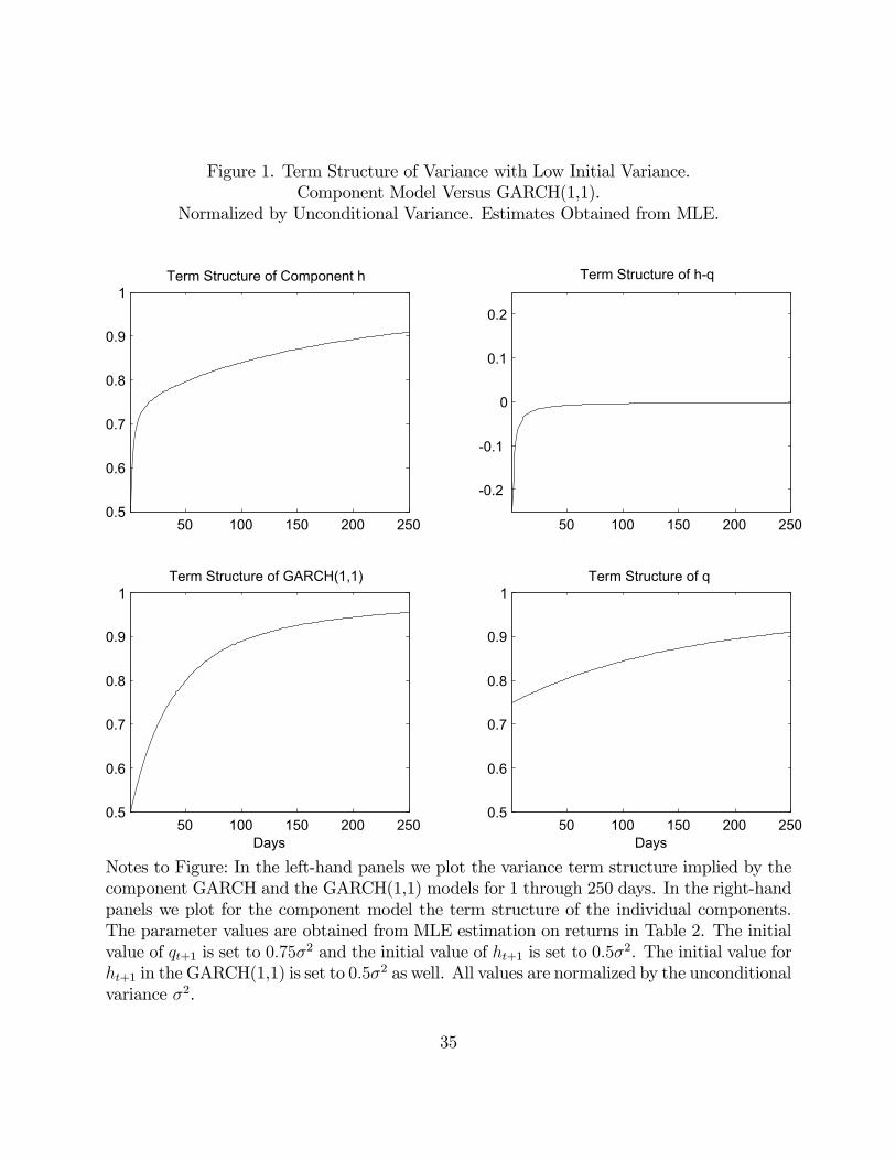
Figure 1. Term Structure of Variance with Low Initial Variance.Component Model Versus GARCH(1,1).

Normalized by Unconditional Variance. Estimates Obtained from MLE.

50 100 150 200 2500.5

0.6

0.7

0.8

0.9

1Term Structure of Component h

50 100 150 200 250

-0.2

-0.1

0

0.1

0.2

Term Structure of h-q

50 100 150 200 2500.5

0.6

0.7

0.8

0.9

1Term Structure of q

Days50 100 150 200 250

0.5

0.6

0.7

0.8

0.9

1Term Structure of GARCH(1,1)

Days

Notes to Figure: In the left-hand panels we plot the variance term structure implied by thecomponent GARCH and the GARCH(1,1) models for 1 through 250 days. In the right-handpanels we plot for the component model the term structure of the individual components.The parameter values are obtained from MLE estimation on returns in Table 2. The initialvalue of qt+1 is set to 0.75σ2 and the initial value of ht+1 is set to 0.5σ2. The initial value forht+1 in the GARCH(1,1) is set to 0.5σ2 as well. All values are normalized by the unconditionalvariance σ2.

35

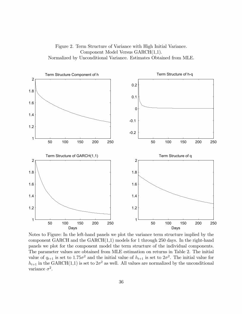
Figure 2. Term Structure of Variance with High Initial Variance.Component Model Versus GARCH(1,1).

Normalized by Unconditional Variance. Estimates Obtained from MLE.

50 100 150 200 2501

1.2

1.4

1.6

1.8

2Term Structure Component of h

50 100 150 200 250

-0.2

-0.1

0

0.1

0.2

Term Structure of h-q

50 100 150 200 2501

1.2

1.4

1.6

1.8

2Term Structure of q

Days50 100 150 200 250

1

1.2

1.4

1.6

1.8

2Term Structure of GARCH(1,1)

Days

Notes to Figure: In the left-hand panels we plot the variance term structure implied by thecomponent GARCH and the GARCH(1,1) models for 1 through 250 days. In the right-handpanels we plot for the component model the term structure of the individual components.The parameter values are obtained from MLE estimation on returns in Table 2. The initialvalue of qt+1 is set to 1.75σ2 and the initial value of ht+1 is set to 2σ2. The initial value forht+1 in the GARCH(1,1) is set to 2σ2 as well. All values are normalized by the unconditionalvariance σ2.

36

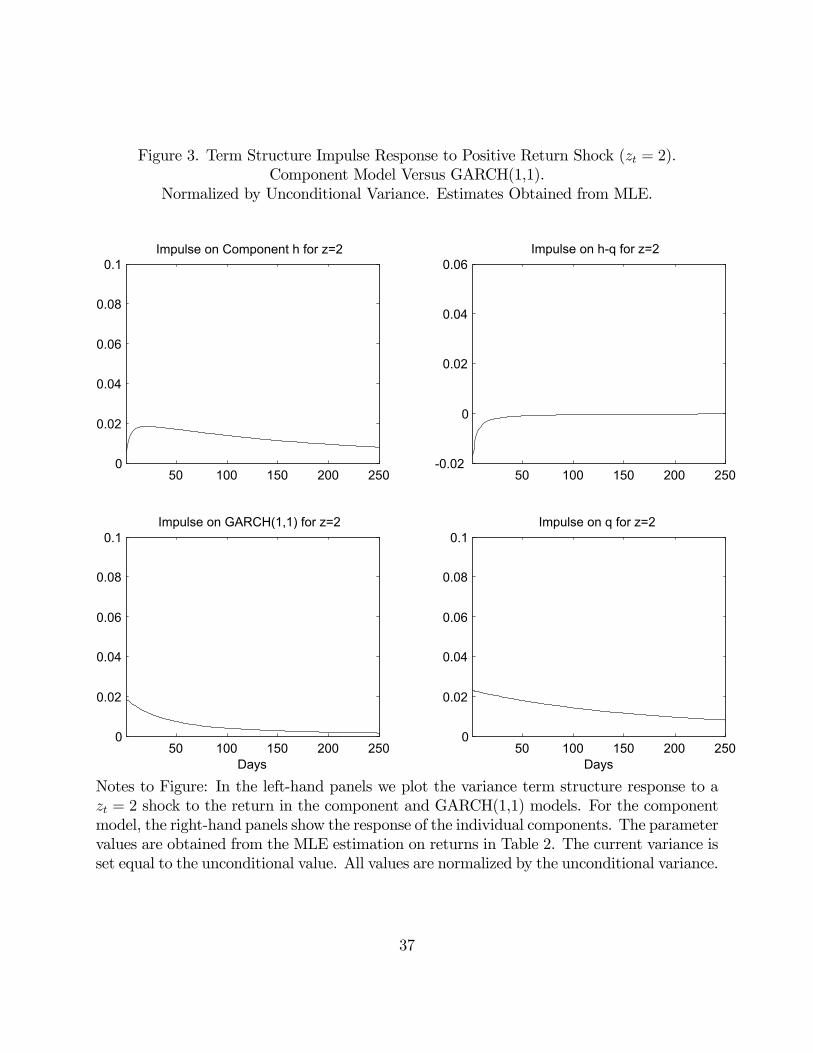
Figure 3. Term Structure Impulse Response to Positive Return Shock (zt = 2).Component Model Versus GARCH(1,1).

Normalized by Unconditional Variance. Estimates Obtained from MLE.

50 100 150 200 2500

0.02

0.04

0.06

0.08

0.1Impulse on Component h for z=2

50 100 150 200 250-0.02

0

0.02

0.04

0.06Impulse on h-q for z=2

50 100 150 200 2500

0.02

0.04

0.06

0.08

0.1Impulse on q for z=2

Days50 100 150 200 250

0

0.02

0.04

0.06

0.08

0.1Impulse on GARCH(1,1) for z=2

Days

Notes to Figure: In the left-hand panels we plot the variance term structure response to azt = 2 shock to the return in the component and GARCH(1,1) models. For the componentmodel, the right-hand panels show the response of the individual components. The parametervalues are obtained from the MLE estimation on returns in Table 2. The current variance isset equal to the unconditional value. All values are normalized by the unconditional variance.

37

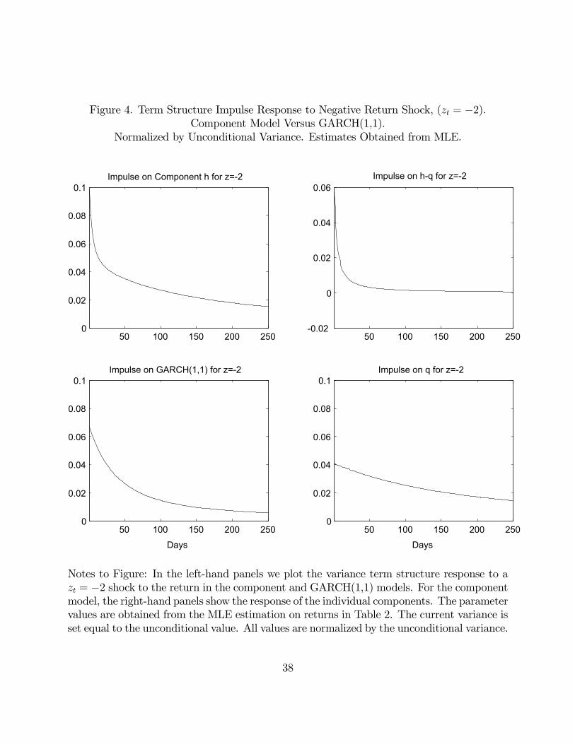
Figure 4. Term Structure Impulse Response to Negative Return Shock, (zt = −2).Component Model Versus GARCH(1,1).

Normalized by Unconditional Variance. Estimates Obtained from MLE.

50 100 150 200 2500

0.02

0.04

0.06

0.08

0.1Impulse on Component h for z=-2

50 100 150 200 250-0.02

0

0.02

0.04

0.06Impulse on h-q for z=-2

50 100 150 200 2500

0.02

0.04

0.06

0.08

0.1Impulse on q for z=-2

Days

50 100 150 200 2500

0.02

0.04

0.06

0.08

0.1Impulse on GARCH(1,1) for z=-2

Days

Notes to Figure: In the left-hand panels we plot the variance term structure response to azt = −2 shock to the return in the component and GARCH(1,1) models. For the componentmodel, the right-hand panels show the response of the individual components. The parametervalues are obtained from the MLE estimation on returns in Table 2. The current variance isset equal to the unconditional value. All values are normalized by the unconditional variance.

38

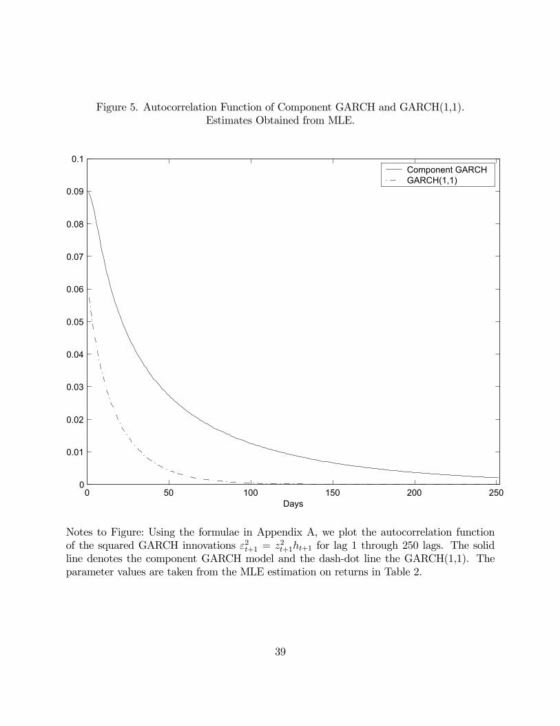
Figure 5. Autocorrelation Function of Component GARCH and GARCH(1,1).Estimates Obtained from MLE.

0 50 100 150 200 2500

0.01

0.02

0.03

0.04

0.05

0.06

0.07

0.08

0.09

0.1

Days

Component GARCHGARCH(1,1)

Notes to Figure: Using the formulae in Appendix A, we plot the autocorrelation functionof the squared GARCH innovations ε2t+1 = z2t+1ht+1 for lag 1 through 250 lags. The solidline denotes the component GARCH model and the dash-dot line the GARCH(1,1). Theparameter values are taken from the MLE estimation on returns in Table 2.

39

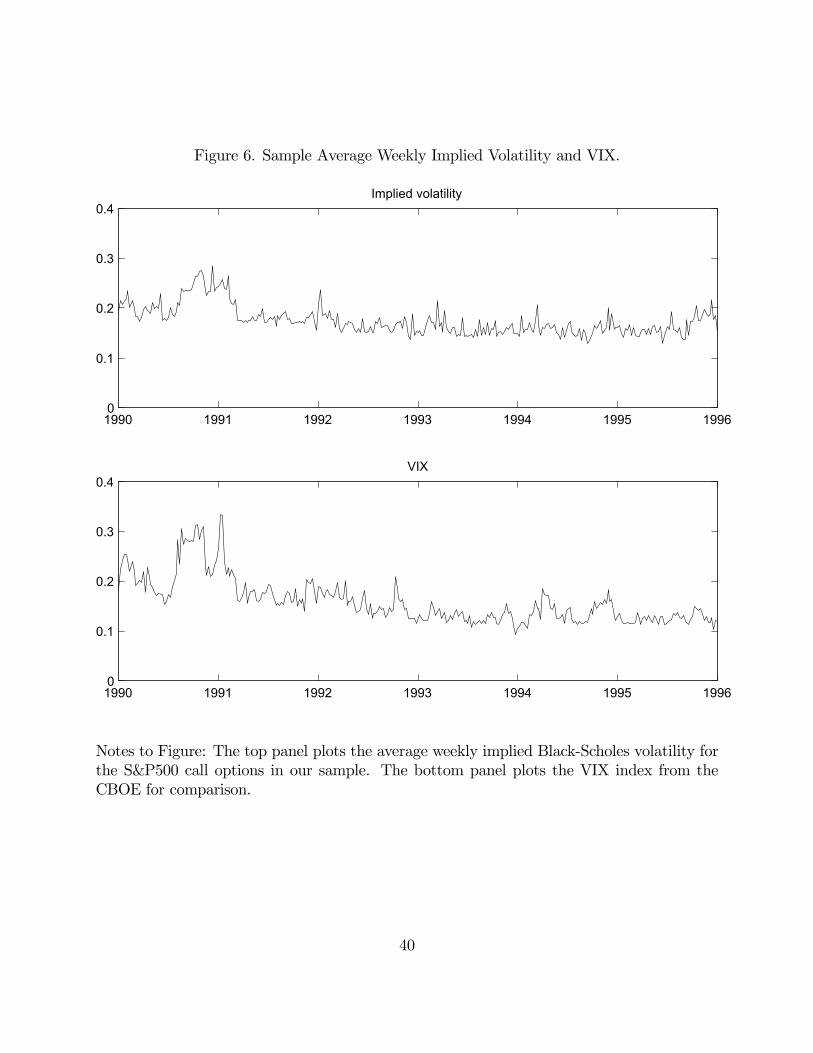
Figure 6. Sample Average Weekly Implied Volatility and VIX.

1990 1991 1992 1993 1994 1995 19960

0.1

0.2

0.3

0.4Implied volatility

1990 1991 1992 1993 1994 1995 19960

0.1

0.2

0.3

0.4VIX

Notes to Figure: The top panel plots the average weekly implied Black-Scholes volatility forthe S&P500 call options in our sample. The bottom panel plots the VIX index from theCBOE for comparison.

40

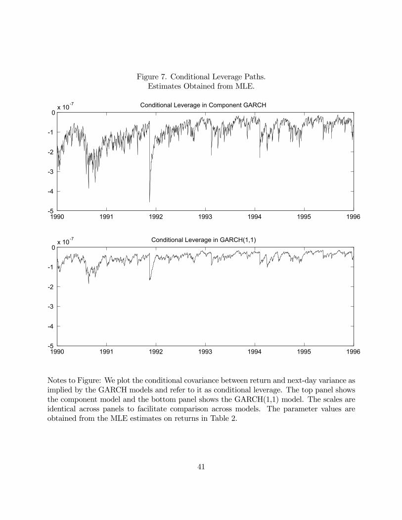
Figure 7. Conditional Leverage Paths.Estimates Obtained from MLE.

1990 1991 1992 1993 1994 1995 1996-5

-4

-3

-2

-1

0x 10-7 Conditional Leverage in Component GARCH

1990 1991 1992 1993 1994 1995 1996-5

-4

-3

-2

-1

0x 10-7 Conditional Leverage in GARCH(1,1)

Notes to Figure: We plot the conditional covariance between return and next-day variance asimplied by the GARCH models and refer to it as conditional leverage. The top panel showsthe component model and the bottom panel shows the GARCH(1,1) model. The scales areidentical across panels to facilitate comparison across models. The parameter values areobtained from the MLE estimates on returns in Table 2.

41

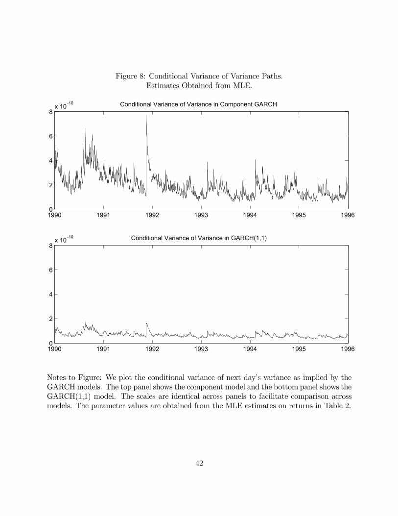
Figure 8: Conditional Variance of Variance Paths.Estimates Obtained from MLE.

1990 1991 1992 1993 1994 1995 19960

2

4

6

8x 10-10 Conditional Variance of Variance in Component GARCH

1990 1991 1992 1993 1994 1995 19960

2

4

6

8x 10-10 Conditional Variance of Variance in GARCH(1,1)

Notes to Figure: We plot the conditional variance of next day’s variance as implied by theGARCHmodels. The top panel shows the component model and the bottom panel shows theGARCH(1,1) model. The scales are identical across panels to facilitate comparison acrossmodels. The parameter values are obtained from the MLE estimates on returns in Table 2.

42

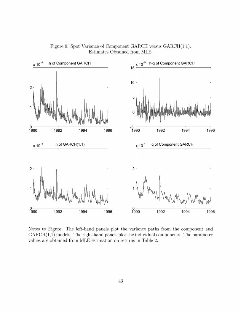
Figure 9. Spot Variance of Component GARCH versus GARCH(1,1).Estimates Obtained from MLE.

1990 1992 1994 19960

1

2

x 10-4 h of Component GARCH

1990 1992 1994 19960

1

2

x 10-4 q of Component GARCH

1990 1992 1994 1996-5

0

5

10

15x 10-5 h-q of Component GARCH

1990 1992 1994 19960

1

2

x 10-4 h of GARCH(1,1)

Notes to Figure: The left-hand panels plot the variance paths from the component andGARCH(1,1) models. The right-hand panels plot the individual components. The parametervalues are obtained from MLE estimation on returns in Table 2.

43

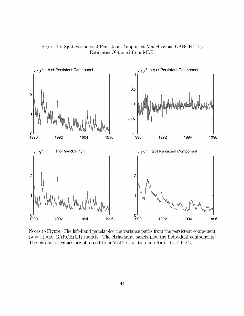
Figure 10. Spot Variance of Persistent Component Model versus GARCH(1,1).Estimates Obtained from MLE.

1990 1992 1994 19960

1

2

x 10-4 h of Persistent Component

1990 1992 1994 19960

1

2

x 10-4 q of Persistent Component

1990 1992 1994 1996-1

-0.5

0

0.5

1x 10-4 h-q of Persistent Component

1990 1992 1994 19960

1

2

x 10-4 h of GARCH(1,1)

Notes to Figure: The left-hand panels plot the variance paths from the persistent component(ρ = 1) and GARCH(1,1) models. The right-hand panels plot the individual components.The parameter values are obtained from MLE estimation on returns in Table 2.

44

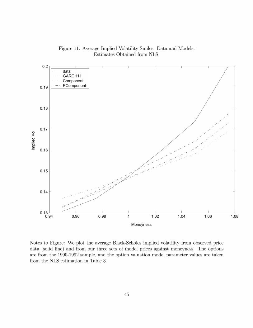
Figure 11. Average Implied Volatility Smiles: Data and Models.Estimates Obtained from NLS.

0.94 0.96 0.98 1 1.02 1.04 1.06 1.080.13

0.14

0.15

0.16

0.17

0.18

0.19

0.2

Moneyness

Impl

ied

Vol

dataGARCH11ComponentPComponent

Notes to Figure: We plot the average Black-Scholes implied volatility from observed pricedata (solid line) and from our three sets of model prices against moneyness. The optionsare from the 1990-1992 sample, and the option valuation model parameter values are takenfrom the NLS estimation in Table 3.

45

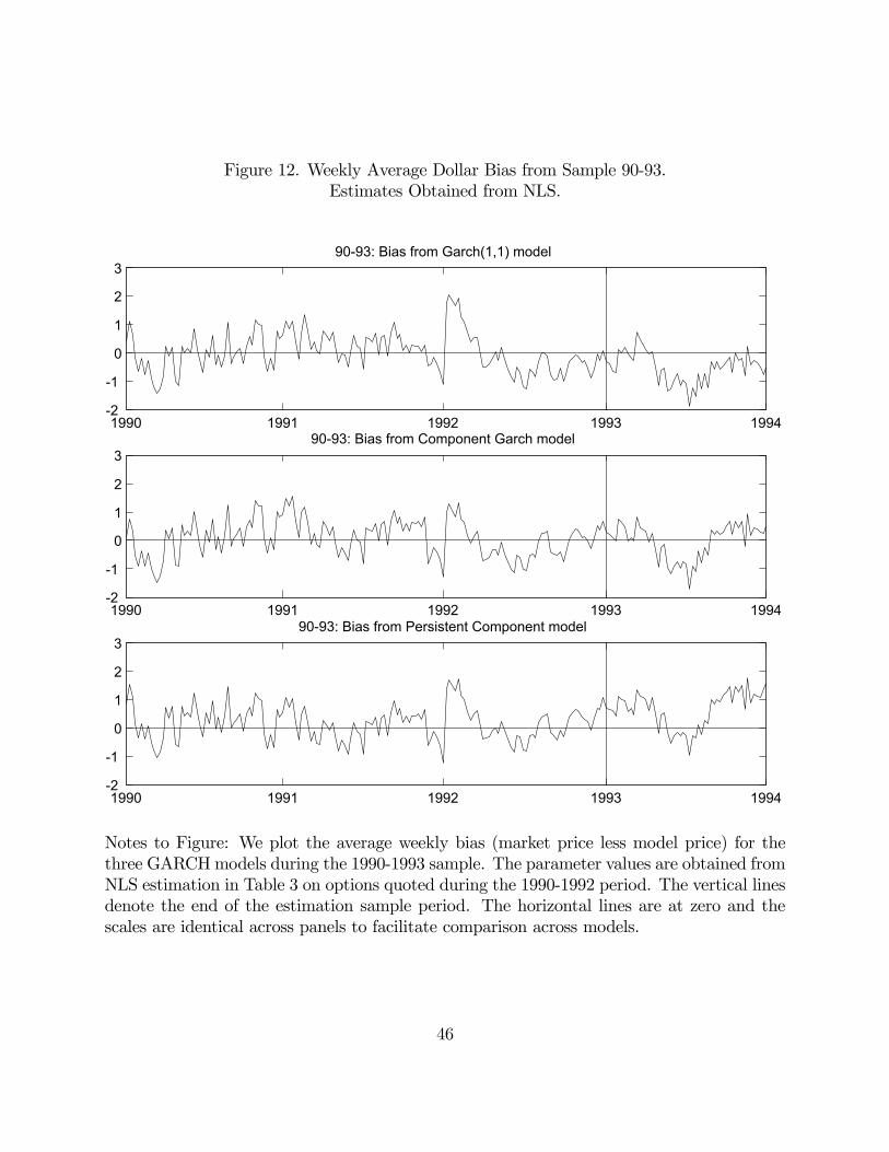
Figure 12. Weekly Average Dollar Bias from Sample 90-93.Estimates Obtained from NLS.

1990 1991 1992 1993 1994-2

-1

0

1

2

390-93: Bias from Garch(1,1) model

1990 1991 1992 1993 1994-2

-1

0

1

2

390-93: Bias from Component Garch model

1990 1991 1992 1993 1994-2

-1

0

1

2

390-93: Bias from Persistent Component model

Notes to Figure: We plot the average weekly bias (market price less model price) for thethree GARCHmodels during the 1990-1993 sample. The parameter values are obtained fromNLS estimation in Table 3 on options quoted during the 1990-1992 period. The vertical linesdenote the end of the estimation sample period. The horizontal lines are at zero and thescales are identical across panels to facilitate comparison across models.

46

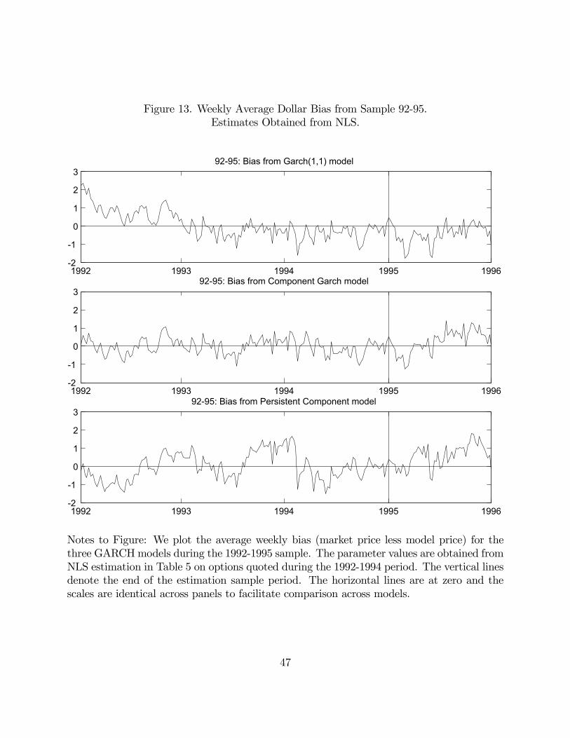
Figure 13. Weekly Average Dollar Bias from Sample 92-95.Estimates Obtained from NLS.

1992 1993 1994 1995 1996-2

-1

0

1

2

392-95: Bias from Garch(1,1) model

1992 1993 1994 1995 1996-2

-1

0

1

2

392-95: Bias from Component Garch model

1992 1993 1994 1995 1996-2

-1

0

1

2

392-95: Bias from Persistent Component model

Notes to Figure: We plot the average weekly bias (market price less model price) for thethree GARCHmodels during the 1992-1995 sample. The parameter values are obtained fromNLS estimation in Table 5 on options quoted during the 1992-1994 period. The vertical linesdenote the end of the estimation sample period. The horizontal lines are at zero and thescales are identical across panels to facilitate comparison across models.

47

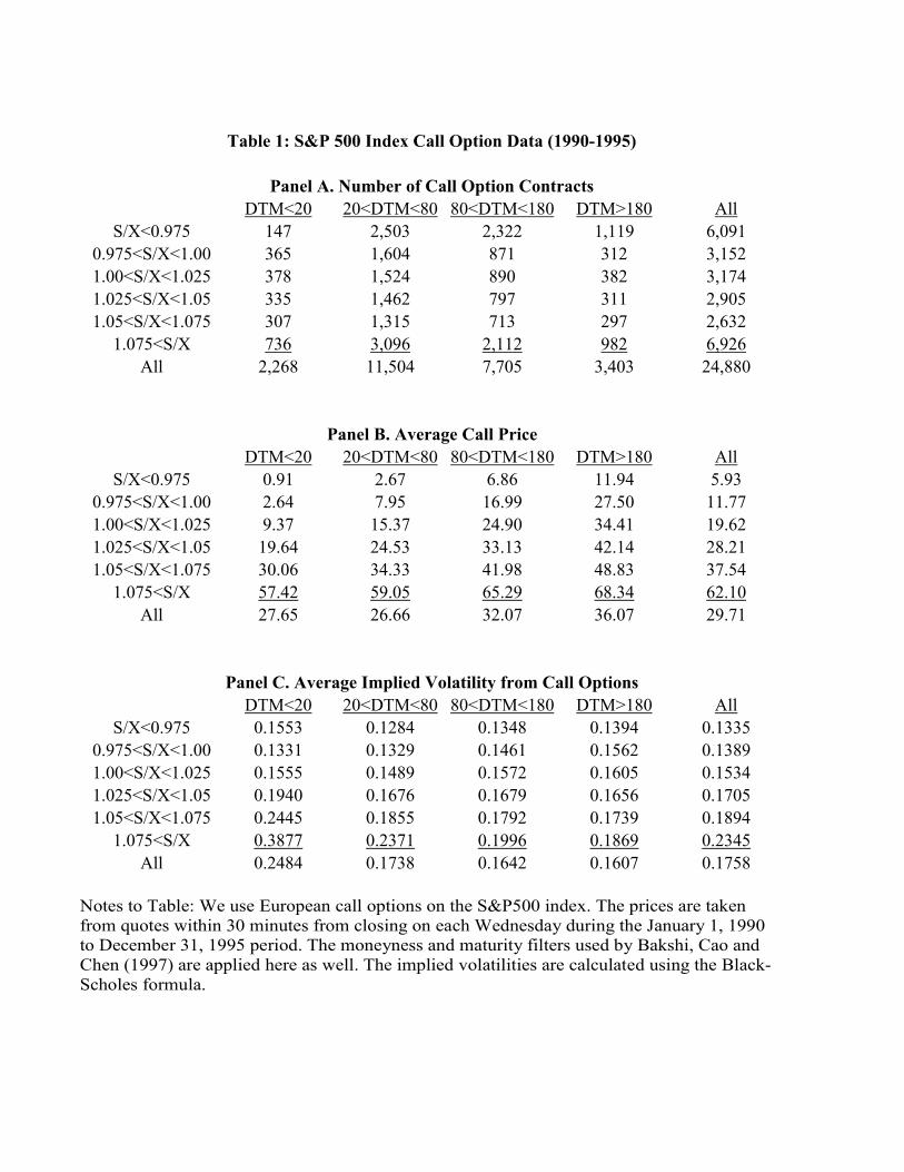
DTM<20 20<DTM<80 80<DTM<180 DTM>180 AllS/X<0.975 147 2,503 2,322 1,119 6,091

0.975<S/X<1.00 365 1,604 871 312 3,1521.00<S/X<1.025 378 1,524 890 382 3,1741.025<S/X<1.05 335 1,462 797 311 2,9051.05<S/X<1.075 307 1,315 713 297 2,632

1.075<S/X 736 3,096 2,112 982 6,926All 2,268 11,504 7,705 3,403 24,880

DTM<20 20<DTM<80 80<DTM<180 DTM>180 AllS/X<0.975 0.91 2.67 6.86 11.94 5.93

0.975<S/X<1.00 2.64 7.95 16.99 27.50 11.771.00<S/X<1.025 9.37 15.37 24.90 34.41 19.621.025<S/X<1.05 19.64 24.53 33.13 42.14 28.211.05<S/X<1.075 30.06 34.33 41.98 48.83 37.54

1.075<S/X 57.42 59.05 65.29 68.34 62.10All 27.65 26.66 32.07 36.07 29.71

DTM<20 20<DTM<80 80<DTM<180 DTM>180 AllS/X<0.975 0.1553 0.1284 0.1348 0.1394 0.1335

0.975<S/X<1.00 0.1331 0.1329 0.1461 0.1562 0.13891.00<S/X<1.025 0.1555 0.1489 0.1572 0.1605 0.15341.025<S/X<1.05 0.1940 0.1676 0.1679 0.1656 0.17051.05<S/X<1.075 0.2445 0.1855 0.1792 0.1739 0.1894

1.075<S/X 0.3877 0.2371 0.1996 0.1869 0.2345All 0.2484 0.1738 0.1642 0.1607 0.1758

Panel A. Number of Call Option Contracts

Panel B. Average Call Price

Panel C. Average Implied Volatility from Call Options

Table 1: S&P 500 Index Call Option Data (1990-1995)

Notes to Table: We use European call options on the S&P500 index. The prices are taken from quotes within 30 minutes from closing on each Wednesday during the January 1, 1990 to December 31, 1995 period. The moneyness and maturity filters used by Bakshi, Cao and Chen (1997) are applied here as well. The implied volatilities are calculated using the Black-Scholes formula.

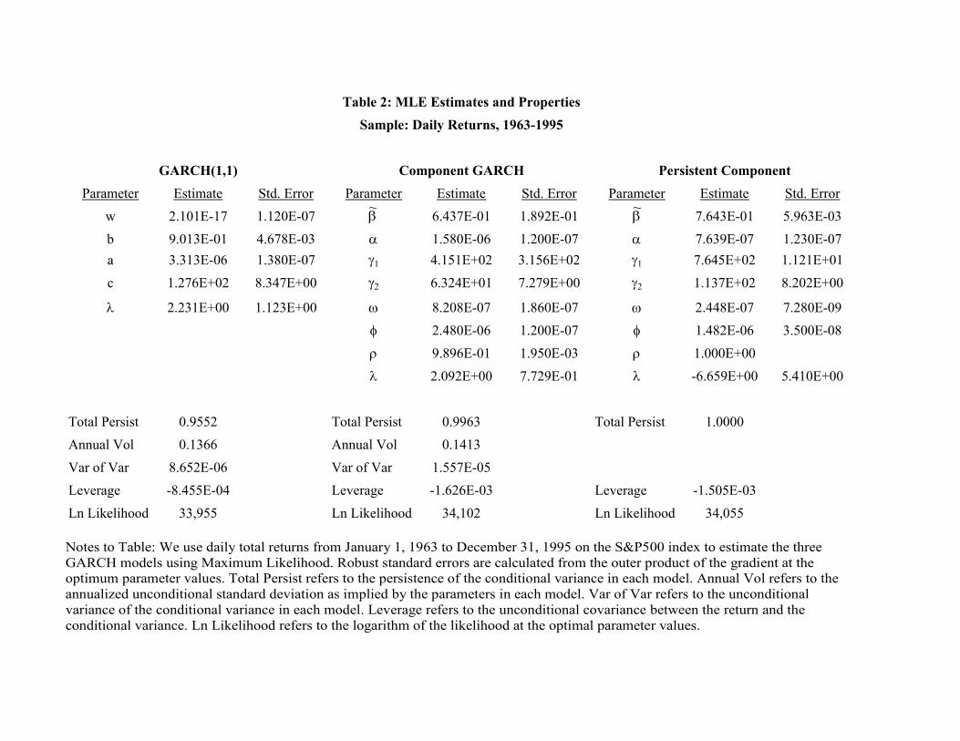
Parameter Estimate Std. Error Parameter Estimate Std. Error Parameter Estimate Std. Errorw 2.101E-17 1.120E-07 6.437E-01 1.892E-01 7.643E-01 5.963E-03b 9.013E-01 4.678E-03 α 1.580E-06 1.200E-07 α 7.639E-07 1.230E-07a 3.313E-06 1.380E-07 γ1 4.151E+02 3.156E+02 γ1 7.645E+02 1.121E+01c 1.276E+02 8.347E+00 γ2 6.324E+01 7.279E+00 γ2 1.137E+02 8.202E+00

λ 2.231E+00 1.123E+00 ω 8.208E-07 1.860E-07 ω 2.448E-07 7.280E-09φ 2.480E-06 1.200E-07 φ 1.482E-06 3.500E-08ρ 9.896E-01 1.950E-03 ρ 1.000E+00λ 2.092E+00 7.729E-01 λ -6.659E+00 5.410E+00

Total Persist 0.9552 Total Persist 0.9963 Total Persist 1.0000Annual Vol 0.1366 Annual Vol 0.1413Var of Var 8.652E-06 Var of Var 1.557E-05Leverage -8.455E-04 Leverage -1.626E-03 Leverage -1.505E-03Ln Likelihood 33,955 Ln Likelihood 34,102 Ln Likelihood 34,055

GARCH(1,1) Component GARCH Persistent Component

Table 2: MLE Estimates and PropertiesSample: Daily Returns, 1963-1995

β~

β~

Notes to Table: We use daily total returns from January 1, 1963 to December 31, 1995 on the S&P500 index to estimate the three GARCH models using Maximum Likelihood. Robust standard errors are calculated from the outer product of the gradient at the optimum parameter values. Total Persist refers to the persistence of the conditional variance in each model. Annual Vol refers to the annualized unconditional standard deviation as implied by the parameters in each model. Var of Var refers to the unconditional variance of the conditional variance in each model. Leverage refers to the unconditional covariance between the return and the conditional variance. Ln Likelihood refers to the logarithm of the likelihood at the optimal parameter values.

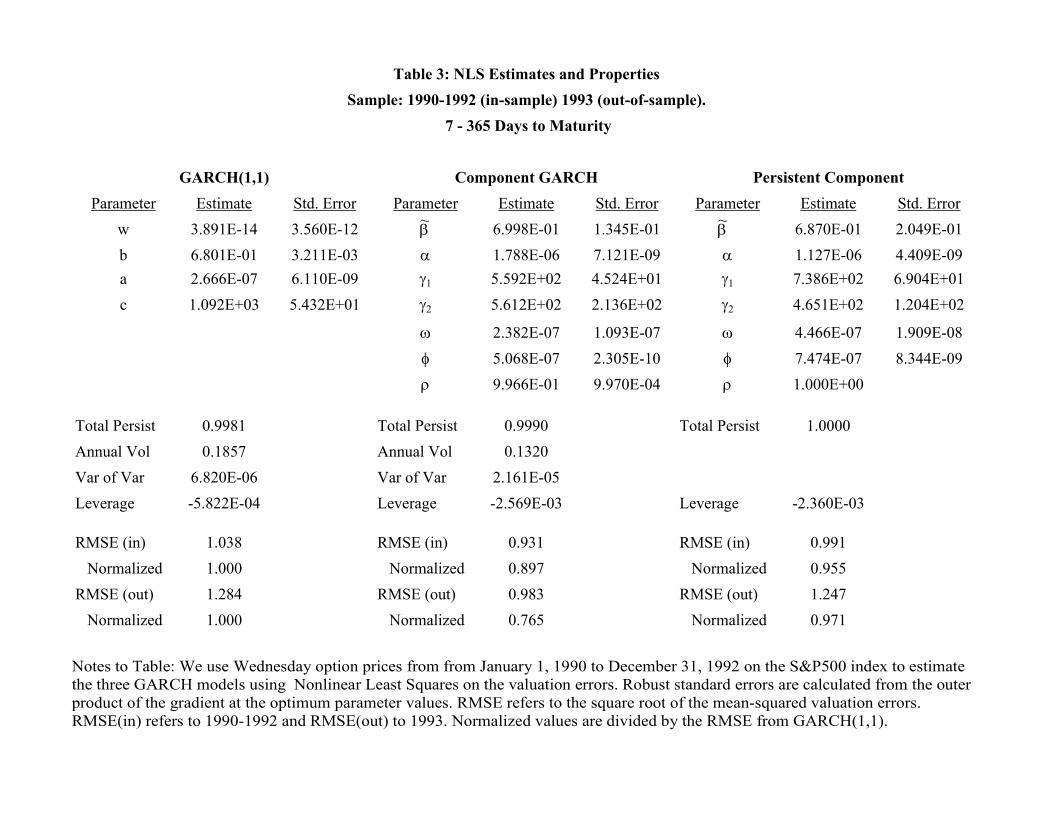
Parameter Estimate Std. Error Parameter Estimate Std. Error Parameter Estimate Std. Errorw 3.891E-14 3.560E-12 6.998E-01 1.345E-01 6.870E-01 2.049E-01b 6.801E-01 3.211E-03 α 1.788E-06 7.121E-09 α 1.127E-06 4.409E-09a 2.666E-07 6.110E-09 γ1 5.592E+02 4.524E+01 γ1 7.386E+02 6.904E+01c 1.092E+03 5.432E+01 γ2 5.612E+02 2.136E+02 γ2 4.651E+02 1.204E+02

ω 2.382E-07 1.093E-07 ω 4.466E-07 1.909E-08φ 5.068E-07 2.305E-10 φ 7.474E-07 8.344E-09ρ 9.966E-01 9.970E-04 ρ 1.000E+00

Total Persist 0.9981 Total Persist 0.9990 Total Persist 1.0000Annual Vol 0.1857 Annual Vol 0.1320Var of Var 6.820E-06 Var of Var 2.161E-05Leverage -5.822E-04 Leverage -2.569E-03 Leverage -2.360E-03

RMSE (in) 1.038 RMSE (in) 0.931 RMSE (in) 0.991 Normalized 1.000 Normalized 0.897 Normalized 0.955RMSE (out) 1.284 RMSE (out) 0.983 RMSE (out) 1.247 Normalized 1.000 Normalized 0.765 Normalized 0.971

GARCH(1,1) Component GARCH Persistent Component

Sample: 1990-1992 (in-sample) 1993 (out-of-sample).Table 3: NLS Estimates and Properties

7 - 365 Days to Maturity

β~

β~

Notes to Table: We use Wednesday option prices from from January 1, 1990 to December 31, 1992 on the S&P500 index to estimate the three GARCH models using Nonlinear Least Squares on the valuation errors. Robust standard errors are calculated from the outer product of the gradient at the optimum parameter values. RMSE refers to the square root of the mean-squared valuation errors. RMSE(in) refers to 1990-1992 and RMSE(out) to 1993. Normalized values are divided by the RMSE from GARCH(1,1).

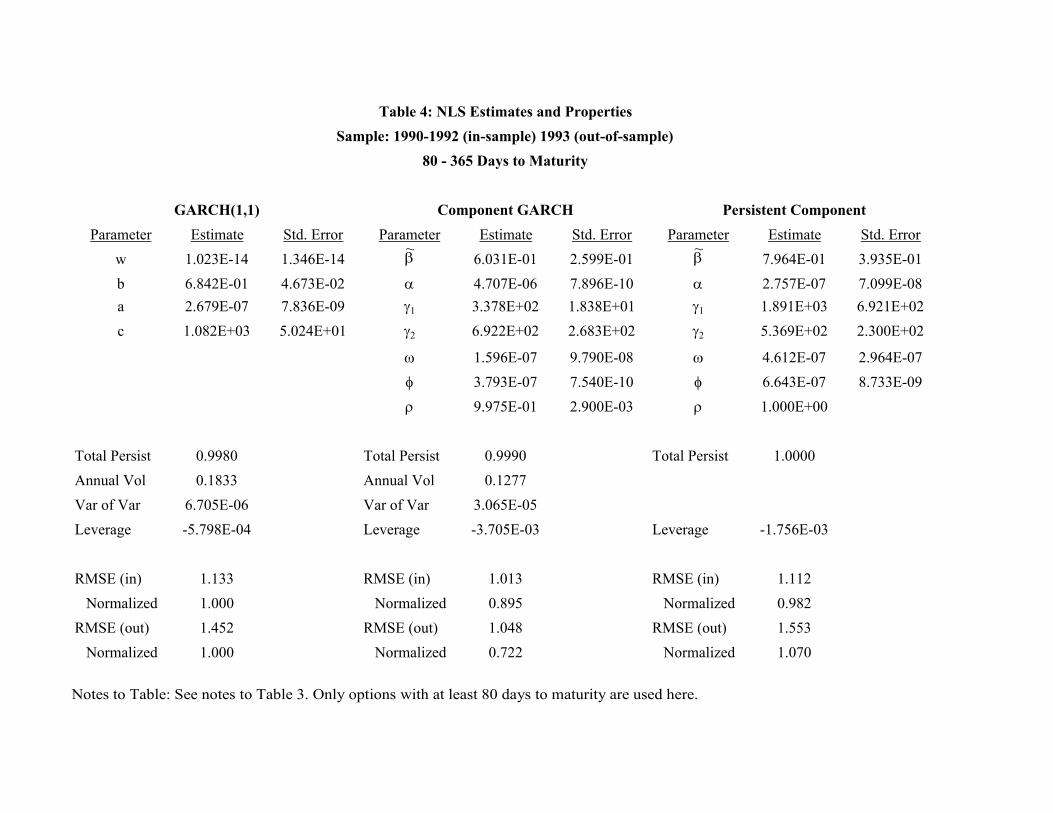
Parameter Estimate Std. Error Parameter Estimate Std. Error Parameter Estimate Std. Errorw 1.023E-14 1.346E-14 6.031E-01 2.599E-01 7.964E-01 3.935E-01b 6.842E-01 4.673E-02 α 4.707E-06 7.896E-10 α 2.757E-07 7.099E-08a 2.679E-07 7.836E-09 γ1 3.378E+02 1.838E+01 γ1 1.891E+03 6.921E+02c 1.082E+03 5.024E+01 γ2 6.922E+02 2.683E+02 γ2 5.369E+02 2.300E+02

ω 1.596E-07 9.790E-08 ω 4.612E-07 2.964E-07φ 3.793E-07 7.540E-10 φ 6.643E-07 8.733E-09ρ 9.975E-01 2.900E-03 ρ 1.000E+00

Total Persist 0.9980 Total Persist 0.9990 Total Persist 1.0000Annual Vol 0.1833 Annual Vol 0.1277Var of Var 6.705E-06 Var of Var 3.065E-05Leverage -5.798E-04 Leverage -3.705E-03 Leverage -1.756E-03

RMSE (in) 1.133 RMSE (in) 1.013 RMSE (in) 1.112 Normalized 1.000 Normalized 0.895 Normalized 0.982RMSE (out) 1.452 RMSE (out) 1.048 RMSE (out) 1.553 Normalized 1.000 Normalized 0.722 Normalized 1.070

Table 4: NLS Estimates and PropertiesSample: 1990-1992 (in-sample) 1993 (out-of-sample)

80 - 365 Days to Maturity

GARCH(1,1) Component GARCH Persistent Component

β~

β~

Notes to Table: See notes to Table 3. Only options with at least 80 days to maturity are used here.

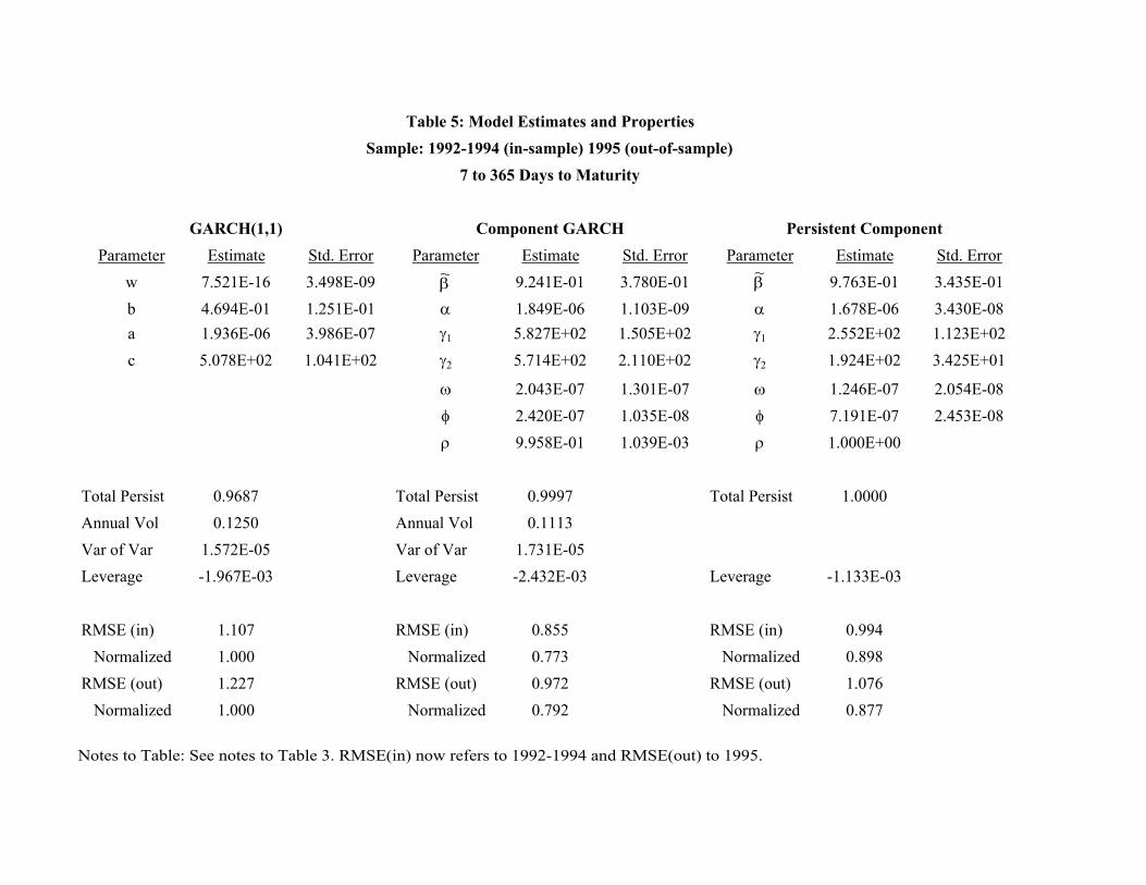
Parameter Estimate Std. Error Parameter Estimate Std. Error Parameter Estimate Std. Errorw 7.521E-16 3.498E-09 9.241E-01 3.780E-01 9.763E-01 3.435E-01b 4.694E-01 1.251E-01 α 1.849E-06 1.103E-09 α 1.678E-06 3.430E-08a 1.936E-06 3.986E-07 γ1 5.827E+02 1.505E+02 γ1 2.552E+02 1.123E+02c 5.078E+02 1.041E+02 γ2 5.714E+02 2.110E+02 γ2 1.924E+02 3.425E+01

ω 2.043E-07 1.301E-07 ω 1.246E-07 2.054E-08φ 2.420E-07 1.035E-08 φ 7.191E-07 2.453E-08ρ 9.958E-01 1.039E-03 ρ 1.000E+00

Total Persist 0.9687 Total Persist 0.9997 Total Persist 1.0000Annual Vol 0.1250 Annual Vol 0.1113Var of Var 1.572E-05 Var of Var 1.731E-05Leverage -1.967E-03 Leverage -2.432E-03 Leverage -1.133E-03

RMSE (in) 1.107 RMSE (in) 0.855 RMSE (in) 0.994 Normalized 1.000 Normalized 0.773 Normalized 0.898RMSE (out) 1.227 RMSE (out) 0.972 RMSE (out) 1.076 Normalized 1.000 Normalized 0.792 Normalized 0.877

Table 5: Model Estimates and PropertiesSample: 1992-1994 (in-sample) 1995 (out-of-sample)

7 to 365 Days to Maturity

GARCH(1,1) Component GARCH Persistent Component

β~ β

~

Notes to Table: See notes to Table 3. RMSE(in) now refers to 1992-1994 and RMSE(out) to 1995.

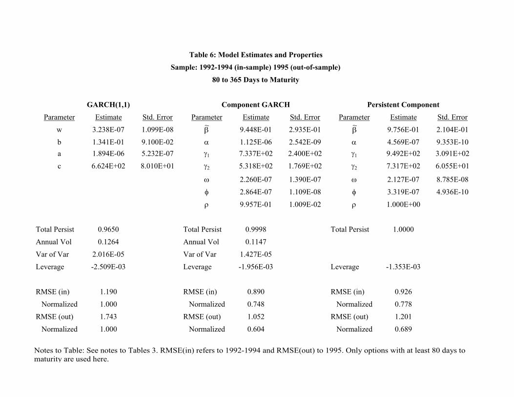
Parameter Estimate Std. Error Parameter Estimate Std. Error Parameter Estimate Std. Errorw 3.238E-07 1.099E-08 9.448E-01 2.935E-01 9.756E-01 2.104E-01b 1.341E-01 9.100E-02 α 1.125E-06 2.542E-09 α 4.569E-07 9.353E-10a 1.894E-06 5.232E-07 γ1 7.337E+02 2.400E+02 γ1 9.492E+02 3.091E+02c 6.624E+02 8.010E+01 γ2 5.318E+02 1.769E+02 γ2 7.317E+02 6.055E+01

ω 2.260E-07 1.390E-07 ω 2.127E-07 8.785E-08φ 2.864E-07 1.109E-08 φ 3.319E-07 4.936E-10ρ 9.957E-01 1.009E-02 ρ 1.000E+00

Total Persist 0.9650 Total Persist 0.9998 Total Persist 1.0000Annual Vol 0.1264 Annual Vol 0.1147Var of Var 2.016E-05 Var of Var 1.427E-05Leverage -2.509E-03 Leverage -1.956E-03 Leverage -1.353E-03

RMSE (in) 1.190 RMSE (in) 0.890 RMSE (in) 0.926 Normalized 1.000 Normalized 0.748 Normalized 0.778RMSE (out) 1.743 RMSE (out) 1.052 RMSE (out) 1.201 Normalized 1.000 Normalized 0.604 Normalized 0.689

GARCH(1,1) Component GARCH Persistent Component

Table 6: Model Estimates and Properties

80 to 365 Days to MaturitySample: 1992-1994 (in-sample) 1995 (out-of-sample)

β~

β~

Notes to Table: See notes to Tables 3. RMSE(in) refers to 1992-1994 and RMSE(out) to 1995. Only options with at least 80 days to maturity are used here.

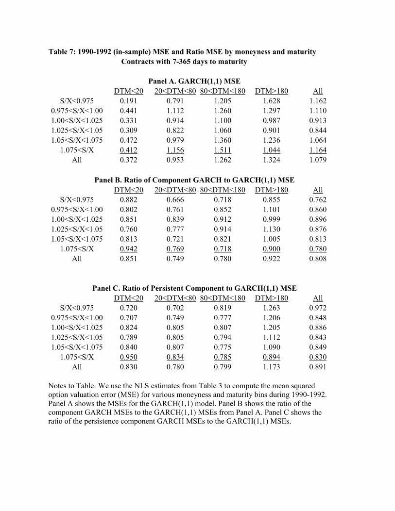
DTM<20 20<DTM<80 80<DTM<180 DTM>180 AllS/X<0.975 0.191 0.791 1.205 1.628 1.162

0.975<S/X<1.00 0.441 1.112 1.260 1.297 1.1101.00<S/X<1.025 0.331 0.914 1.100 0.987 0.9131.025<S/X<1.05 0.309 0.822 1.060 0.901 0.8441.05<S/X<1.075 0.472 0.979 1.360 1.236 1.064

1.075<S/X 0.412 1.156 1.511 1.044 1.164All 0.372 0.953 1.262 1.324 1.079

DTM<20 20<DTM<80 80<DTM<180 DTM>180 AllS/X<0.975 0.882 0.666 0.718 0.855 0.762

0.975<S/X<1.00 0.802 0.761 0.852 1.101 0.8601.00<S/X<1.025 0.851 0.839 0.912 0.999 0.8961.025<S/X<1.05 0.760 0.777 0.914 1.130 0.8761.05<S/X<1.075 0.813 0.721 0.821 1.005 0.813

1.075<S/X 0.942 0.769 0.718 0.900 0.780All 0.851 0.749 0.780 0.922 0.808

DTM<20 20<DTM<80 80<DTM<180 DTM>180 AllS/X<0.975 0.720 0.702 0.819 1.263 0.972

0.975<S/X<1.00 0.707 0.749 0.777 1.206 0.8481.00<S/X<1.025 0.824 0.805 0.807 1.205 0.8861.025<S/X<1.05 0.789 0.805 0.794 1.112 0.8431.05<S/X<1.075 0.840 0.807 0.775 1.090 0.849

1.075<S/X 0.950 0.834 0.785 0.894 0.830All 0.830 0.780 0.799 1.173 0.891

Table 7: 1990-1992 (in-sample) MSE and Ratio MSE by moneyness and maturity Contracts with 7-365 days to maturity

Panel A. GARCH(1,1) MSE

Panel B. Ratio of Component GARCH to GARCH(1,1) MSE

Panel C. Ratio of Persistent Component to GARCH(1,1) MSE

Notes to Table: We use the NLS estimates from Table 3 to compute the mean squared option valuation error (MSE) for various moneyness and maturity bins during 1990-1992. Panel A shows the MSEs for the GARCH(1,1) model. Panel B shows the ratio of the component GARCH MSEs to the GARCH(1,1) MSEs from Panel A. Panel C shows the ratio of the persistence component GARCH MSEs to the GARCH(1,1) MSEs.

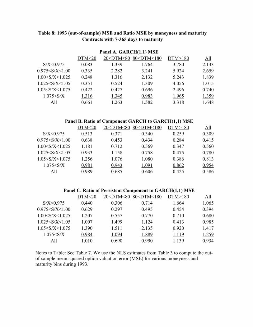
DTM<20 20<DTM<80 80<DTM<180 DTM>180 AllS/X<0.975 0.083 1.339 1.764 3.780 2.133

0.975<S/X<1.00 0.335 2.282 3.241 5.924 2.6591.00<S/X<1.025 0.248 1.316 2.132 5.243 1.8391.025<S/X<1.05 0.351 0.524 1.309 4.056 1.0151.05<S/X<1.075 0.422 0.427 0.696 2.496 0.740

1.075<S/X 1.316 1.345 0.983 1.965 1.359All 0.661 1.263 1.582 3.318 1.648

DTM<20 20<DTM<80 80<DTM<180 DTM>180 AllS/X<0.975 0.513 0.371 0.340 0.259 0.309

0.975<S/X<1.00 0.638 0.453 0.434 0.284 0.4151.00<S/X<1.025 1.181 0.712 0.569 0.347 0.5601.025<S/X<1.05 0.933 1.158 0.758 0.475 0.7801.05<S/X<1.075 1.256 1.076 1.080 0.386 0.813

1.075<S/X 0.981 0.943 1.091 0.862 0.954All 0.989 0.685 0.606 0.425 0.586

DTM<20 20<DTM<80 80<DTM<180 DTM>180 AllS/X<0.975 0.440 0.306 0.714 1.664 1.065

0.975<S/X<1.00 0.629 0.297 0.495 0.454 0.3941.00<S/X<1.025 1.207 0.557 0.770 0.710 0.6801.025<S/X<1.05 1.007 1.499 1.124 0.413 0.9851.05<S/X<1.075 1.390 1.511 2.135 0.920 1.417

1.075<S/X 0.984 1.094 1.889 1.119 1.259All 1.010 0.690 0.990 1.139 0.934

Panel C. Ratio of Persistent Component to GARCH(1,1) MSE

Table 8: 1993 (out-of-sample) MSE and Ratio MSE by moneyness and maturityContracts with 7-365 days to maturity

Panel A. GARCH(1,1) MSE

Panel B. Ratio of Component GARCH to GARCH(1,1) MSE

Notes to Table: See Table 7. We use the NLS estimates from Table 3 to compute the out-of-sample mean squared option valuation error (MSE) for various moneyness and maturity bins during 1993.

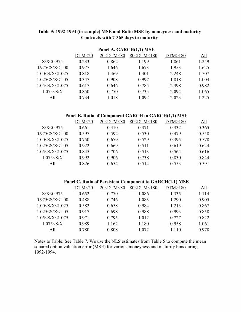
DTM<20 20<DTM<80 80<DTM<180 DTM>180 AllS/X<0.975 0.233 0.862 1.199 1.861 1.259

0.975<S/X<1.00 0.977 1.646 1.673 1.953 1.6251.00<S/X<1.025 0.818 1.469 1.401 2.248 1.5071.025<S/X<1.05 0.347 0.908 0.997 1.818 1.0041.05<S/X<1.075 0.617 0.646 0.785 2.398 0.982

1.075<S/X 0.850 0.750 0.735 2.094 1.065All 0.734 1.018 1.092 2.023 1.225

DTM<20 20<DTM<80 80<DTM<180 DTM>180 AllS/X<0.975 0.661 0.410 0.371 0.332 0.365

0.975<S/X<1.00 0.597 0.592 0.530 0.479 0.5581.00<S/X<1.025 0.750 0.679 0.529 0.395 0.5781.025<S/X<1.05 0.922 0.669 0.511 0.619 0.6241.05<S/X<1.075 0.845 0.706 0.513 0.564 0.616

1.075<S/X 0.992 0.906 0.738 0.830 0.844All 0.826 0.654 0.514 0.553 0.591

DTM<20 20<DTM<80 80<DTM<180 DTM>180 AllS/X<0.975 0.652 0.770 1.086 1.335 1.114

0.975<S/X<1.00 0.488 0.746 1.083 1.290 0.9051.00<S/X<1.025 0.582 0.658 0.984 1.213 0.8671.025<S/X<1.05 0.917 0.698 0.988 0.993 0.8581.05<S/X<1.075 0.971 0.795 1.012 0.727 0.822

1.075<S/X 0.989 1.162 1.180 0.958 1.061All 0.780 0.808 1.072 1.110 0.978

Panel C. Ratio of Persistent Component to GARCH(1,1) MSE

Table 9: 1992-1994 (in-sample) MSE and Ratio MSE by moneyness and maturityContracts with 7-365 days to maturity

Panel A. GARCH(1,1) MSE

Panel B. Ratio of Component GARCH to GARCH(1,1) MSE

Notes to Table: See Table 7. We use the NLS estimates from Table 5 to compute the mean squared option valuation error (MSE) for various moneyness and maturity bins during 1992-1994.

DTM<20 20<DTM<80 80<DTM<180 DTM>180 AllS/X<0.975 0.150 0.745 2.120 6.033 3.135

0.975<S/X<1.00 0.991 1.381 2.954 4.381 2.3911.00<S/X<1.025 0.566 1.134 2.292 3.505 1.9301.025<S/X<1.05 0.289 0.827 1.599 2.103 1.2331.05<S/X<1.075 0.816 0.380 0.751 1.963 0.803

1.075<S/X 0.415 0.380 0.326 0.929 0.463All 0.553 0.716 1.408 3.415 1.507

DTM<20 20<DTM<80 80<DTM<180 DTM>180 AllS/X<0.975 1.700 1.404 0.947 0.378 0.572

0.975<S/X<1.00 0.988 0.815 0.571 0.481 0.6131.00<S/X<1.025 0.703 0.562 0.543 0.424 0.5011.025<S/X<1.05 1.074 0.559 0.432 0.465 0.4971.05<S/X<1.075 0.959 0.691 0.588 0.550 0.634

1.075<S/X 1.016 1.160 1.190 0.870 1.052All 0.957 0.863 0.717 0.449 0.613

DTM<20 20<DTM<80 80<DTM<180 DTM>180 AllS/X<0.975 0.749 0.987 0.647 0.372 0.475

0.975<S/X<1.00 0.824 0.780 0.564 0.660 0.6701.00<S/X<1.025 0.748 0.678 0.675 0.605 0.6481.025<S/X<1.05 1.216 0.899 0.671 0.712 0.7671.05<S/X<1.075 1.059 1.492 1.364 0.641 1.041

1.075<S/X 0.927 1.753 2.457 1.099 1.589All 0.922 1.034 0.822 0.536 0.718

Panel C. Ratio of Persistent Component to GARCH(1,1) MSE

Table 10: 1995 (out-of-sample) MSE and Ratio MSE by moneyness and maturityContracts with 7-365 days to maturity

Panel A. GARCH(1,1)

Panel B. Ratio of Component GARCH to GARCH(1,1) MSE

Notes to Table: See Table 7. We use the NLS estimates from Table 5 to compute the out-of-sample mean squared option valuation error (MSE) for various moneyness and maturity bins during 1995.