Options and Strategies for Fiscal Consolidation in India

Sampawende J.-A. Tapsoba

WP/13/127

© 2013 International Monetary Fund WP/13/127

IMF Working Paper

Asia and Pacific Department

Options and Strategies for Fiscal Consolidation in India1

Prepared by Sampawende J.-A. Tapsoba

Authorized for distribution by Laura Papi

May 2013

Abstract

The paper uses a multi-region DSGE model to quantify the macroeconomic implications of three adjustment scenarios for India: growth-friendly, social-friendly, and a benchmark case centered on bringing down unproductive spending and strengthening the consumption tax. Simulations indicate that fiscal consolidation yields considerable long-term benefits but also entails output costs in the near term. The scenarios in which deficit reduction is accompanied by greater investment and social spending lead to better results than the benchmark case. The consolidation package alone is not enough to maximize net gains. Other factors, such as the pace and the credibility of consolidation, the concomitant implementation of structural reforms, and global economic conditions, play a critical role in the success of fiscal consolidation.

JEL Classification Numbers: E62, F41 H62, H63.

Keywords: fiscal consolidation, open economy macroeconomics, DSGE models, India.

Author’s E-Mail Address: stapsoba@imf.org.

1 I thank, without implication, Emre Alper, Derek Anderson, Marialuz Moreno-Badia, Laura Papi, Andrea Schaechter, Jose Torres, James P. Walsh, Anke Weber, and the participants of the International Conference on Contemporary Debates in Public Policy and Management (IIM Calcutta, India on February 7–9, 2013) for their invaluable comments and suggestions, and Debra Loucks, May Inoue, and Rosanne Heller for their editorial assistance.

This Working Paper should not be reported as representing the views of the IMF. The views expressed in this Working Paper are those of the author(s) and do not necessarily represent those of the IMF or IMF policy. Working Papers describe research in progress by the author(s) and are published to elicit comments and to further debate.

2

Contents Page

I. Introduction ............................................................................................................................3

II. Model and Calibration ...........................................................................................................4

III. Consolidation Strategies ......................................................................................................8

IV. Policy Simulations .............................................................................................................10 A. Baseline Simulations .....................................................................................................10 B. Additional Simulations ..................................................................................................12

V. Conclusion ..........................................................................................................................19

References ................................................................................................................................21

Figures 1. Gradual Fiscal Consolidation ...............................................................................................13 2. Front-loaded Consolidation .................................................................................................15 3. Stop-and-Go Fiscal Consolidation .......................................................................................16 4. Credibility of Fiscal Consolidation ......................................................................................17 5. Domestic Structural Reforms and Fiscal Consolidation ......................................................18 6. Fiscal Consolidation and Inward Spillovers ........................................................................18 Tables 1. Fiscal Consolidation Scenarios ..............................................................................................9 2. Impact of Fiscal Consolidation on Real GDP by Instrument ..............................................11 3. First-Year Fiscal Multipliers: India and Selected Regions ..................................................11 Appendix Tables 1. GIMF Dynamic Model Calibration .....................................................................................23 2. GIMF Steady-state Calibration—Macroeconomic Variables ..............................................24 3. GIMF Steady-state Calibration—Country Sizes and Nominal Trade Matrix .....................25 

3

I. INTRODUCTION

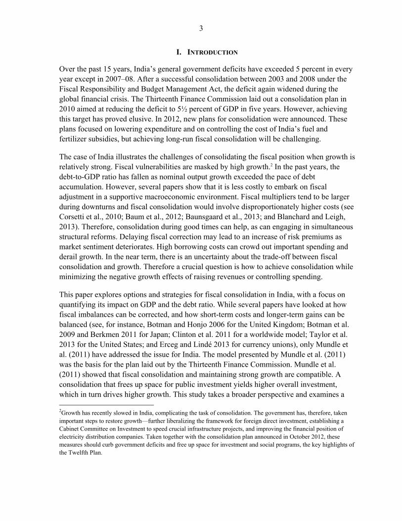
Over the past 15 years, India’s general government deficits have exceeded 5 percent in every year except in 2007–08. After a successful consolidation between 2003 and 2008 under the Fiscal Responsibility and Budget Management Act, the deficit again widened during the global financial crisis. The Thirteenth Finance Commission laid out a consolidation plan in 2010 aimed at reducing the deficit to 5½ percent of GDP in five years. However, achieving this target has proved elusive. In 2012, new plans for consolidation were announced. These plans focused on lowering expenditure and on controlling the cost of India’s fuel and fertilizer subsidies, but achieving long-run fiscal consolidation will be challenging.

The case of India illustrates the challenges of consolidating the fiscal position when growth is relatively strong. Fiscal vulnerabilities are masked by high growth.2 In the past years, the debt-to-GDP ratio has fallen as nominal output growth exceeded the pace of debt accumulation. However, several papers show that it is less costly to embark on fiscal adjustment in a supportive macroeconomic environment. Fiscal multipliers tend to be larger during downturns and fiscal consolidation would involve disproportionately higher costs (see Corsetti et al., 2010; Baum et al., 2012; Baunsgaard et al., 2013; and Blanchard and Leigh, 2013). Therefore, consolidation during good times can help, as can engaging in simultaneous structural reforms. Delaying fiscal correction may lead to an increase of risk premiums as market sentiment deteriorates. High borrowing costs can crowd out important spending and derail growth. In the near term, there is an uncertainty about the trade-off between fiscal consolidation and growth. Therefore a crucial question is how to achieve consolidation while minimizing the negative growth effects of raising revenues or controlling spending.

This paper explores options and strategies for fiscal consolidation in India, with a focus on quantifying its impact on GDP and the debt ratio. While several papers have looked at how fiscal imbalances can be corrected, and how short-term costs and longer-term gains can be balanced (see, for instance, Botman and Honjo 2006 for the United Kingdom; Botman et al. 2009 and Berkmen 2011 for Japan; Clinton et al. 2011 for a worldwide model; Taylor et al. 2013 for the United States; and Erceg and Lindé 2013 for currency unions), only Mundle et al. (2011) have addressed the issue for India. The model presented by Mundle et al. (2011) was the basis for the plan laid out by the Thirteenth Finance Commission. Mundle et al. (2011) showed that fiscal consolidation and maintaining strong growth are compatible. A consolidation that frees up space for public investment yields higher overall investment, which in turn drives higher growth. This study takes a broader perspective and examines a 2Growth has recently slowed in India, complicating the task of consolidation. The government has, therefore, taken important steps to restore growth—further liberalizing the framework for foreign direct investment, establishing a Cabinet Committee on Investment to speed crucial infrastructure projects, and improving the financial position of electricity distribution companies. Taken together with the consolidation plan announced in October 2012, these measures should curb government deficits and free up space for investment and social programs, the key highlights of the Twelfth Plan.

4

more comprehensive fiscal consolidation framework. It analyzes three scenarios to curtail the debt ratio. A growth-friendly scenario and a social-friendly scenario are compared to a benchmark consolidation based on lowering unproductive expenditure and strengthening consumption tax revenue. Several dimensions of the implementation, such as the speed and the credibility, along with structural reforms and varying global economic conditions, are also explored.

For the purpose of this study, the IMF Global Integrated Monetary and Fiscal model (GIMF) is used to explore options and strategies for fiscal adjustment. GIMF is a dynamic stochastic general equilibrium (DSGE) multi-region model with microeconomic foundations and non-Ricardian features. It includes a detailed fiscal sector that is well suited for a comprehensive analysis of factors that lead to successful fiscal consolidation. The multi-country dimension of GIMF also allows an assessment of the role of external shocks (e.g., see Clinton et al., 2011). The regions are intertwined through a rich multilateral trade matrix. The model is calibrated to the Indian economy, the euro area, and the rest of the world.3

The remainder of the paper is structured as follows. The next section describes the key features of GIMF. Section 3 lays out the different fiscal strategies and scenarios. Section 4 presents and discusses the simulations. It first compares the impact on growth of the benchmark, growth-friendly, and social-friendly scenarios. It then assesses multipliers of the different fiscal instruments, looking at both short- and long-run horizons. Finally, variations on the growth-friendly scenario are simulated to assess the effects of different timetables, the extent of policy credibility, the presence of domestic structural reform, and varying global economic conditions on the success of fiscal consolidation. The final section concludes with policy recommendations.

II. MODEL AND CALIBRATION

GIMF is a multi-region DSGE model that integrates supply, demand, trade, and international asset markets into a single theoretical framework. In GIMF, unions, manufacturers, and distributors face nominal rigidity in price setting, while retailers and importers are subject to real rigidities, as it is costly to rapidly adjust their sales volume. Manufacturers are also subject to real rigidity in capital accumulation. All parameters except population and technology growth can differ across economies. For the sake of brevity, only the key equations of the model are presented. A full description of the theoretical model and its calibration can be found in Kumhof et al. (2010).

3 Following Clinton et al. (2011), a six-region version of GIMF (comprising India, the euro area, Emerging Asia— China, Hong Kong SAR, India, Indonesia, the Republic of Korea, Malaysia, Philippines, Singapore, and Thailand—Japan, the United States, and the rest of the world) has been used to test the robustness of the simulations. Overall, findings are similar with those discussed in the paper. For the sake of brevity and because fiscal consolidation is mainly a domestic issue, the present study is based on the simulations from the three- region version. Moreover, the euro area is singled out because of the recent concerns over spillovers to India from an intensification of the crisis in this region.

5

Household sector

Each economy is populated with two types of households, overlapping generations (OLG) households and liquidity-constrained (LIQ) households. The main difference between these two types of households is that the latter do not have access to financial markets and are forced to consume their after-tax income each period. OLG households save by acquiring domestic government bonds denominated in domestic currency and foreign bonds denominated in U.S. dollars. The OLG households also receive labor and dividend income. They maximize their utility subject to their budgetary constraints. Aggregate consumption for OLG households is a function of financial wealth, and the present discounted value of after-tax wage and investment income. The optimization problem of LIQ households is similar to that of OLG households, except that LIQ households do not hold financial assets. Respective optimal quantities of the different consumers in the economy are added to obtain aggregate consumption demand and labor supply.

Production sector

Production in GIMF is multilayered. Capital and labor produce tradable and nontradable goods. Capital is supplied by entrepreneurs with a procyclical financial accelerator a la Bernanke et al. (1999). Unions buy labor services from the two types of households and sell them to manufacturers; the latter purchase investment goods from distributors and use the two production factors to produce intermediate tradable and nontradable goods. The intermediate goods are then sold to domestic distributors and import agents of foreign economies. Firms that produce tradable and nontradable intermediate goods are managed in accordance with, preferences of their owners, finitely-lived households. Firms are subject to nominal rigidities in price setting, as well as real adjustment costs in labor hiring and investment. They pay capital income taxes to governments and wages and dividends to households. Labor is mobile across sectors but not countries; capital is sector-specific and is also immobile across countries. Firms also use public infrastructure (government capital stock) as an input, in combination with tradable and nontradable intermediate goods. Therefore, government capital adds to the productivity of the economy.

Fiscal and monetary policies

Conventional DSGE models assume Ricardian households, which weakens the potential for fiscal policy analysis. GIMF, however, has non-Ricardian features, making fiscal policy matter both in the short and long term. There are many ways that the fiscal authority can interact with the economy. Fiscal policy consists of a specification of public investment spending, public consumption spending, lump-sum taxes, lump-sum transfers, and three different distortionary taxes (labor tax, consumption tax, and capital tax). Fiscal policy is governed by the following structural fiscal balance rule:

  (1)

6

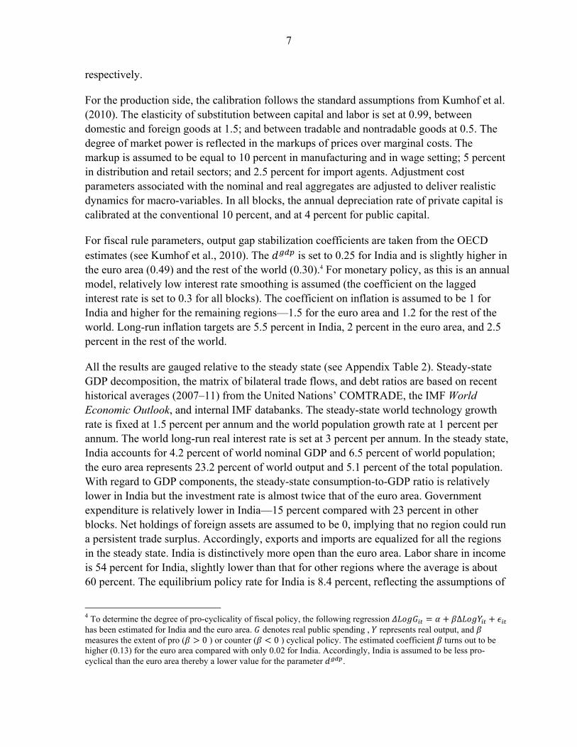
where represents the government surplus-to-GDP ratio and is the long-run

target of . and denote real GDP and potential real GDP, respectively. is a positive parameter and captures the automatic stabilizer component of fiscal policy.

The rule stabilizes the government surplus and the business cycle by adjusting tax rates or expenditure. First, it stabilizes the interest-inclusive government surplus-to-GDP ratio at the long-run target level, , thereby ruling out default and fiscal dominance. Second, it stabilizes the business cycle by letting the surplus evolve with the output gap term,

.

In this paper, monetary policy aims at stabilizing inflation through a Taylor-type rule that features interest rate smoothing and responds to the deviations of expected year-on-year

inflation from the inflation target , with denoting the inflation objective, which can

be subject to unit root shocks. Furthermore, the rule allows for discretionary and autocorrelated monetary policy shocks, . The rule takes the following form:

, (2)

where is the short-term policy interest rate and is the equilibrium real world interest rate. is a proxy of the gross nominal interest rate. and are non-negative parameters and denote the weights on the lagged interest rate and the inflation gap, respectively.

Calibration

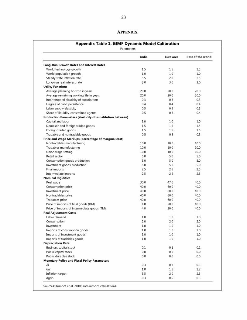
Calibrating GIMF requires detailed data on the national accounts, the labor shares in the tradable and nontradable sectors, the external position, the trade structure, the fiscal position, and the inflation target. For this paper, a three-region version is calibrated for India, with the euro area, and the rest of the world. The main behavioral parameters (see Appendix Table 1) have been determined in accordance with the existing literature and empirical evidence gathered in previous papers using GIMF (Kumhof et al., 2010; and Clinton et al., 2011).

Households’ utility functions are the same across countries. Based on the empirical evidence of the effect of government debt on real interest rates, the planning horizon or the degree of myopia of households and the remaining time at work are respectively set to 20 years. Household preferences are further characterized by an intertemporal elasticity of substitution of 0.25. The Frisch elasticity of labor supply of both OLG and LIQ households is adjusted to obtain an elasticity of 0.5, in line with the business cycle literature. The planning horizon, the remaining time at work, the intertemporal elasticity of substitution, and the elasticity of labor supply are critical for the non-Ricardian behavior of the model. To reflect the stage of financial development, the shares of consumers facing liquidity constraints are set to 50 percent in India, 25 percent in the euro area, and 40 percent in the rest of the world,

7

respectively.

For the production side, the calibration follows the standard assumptions from Kumhof et al. (2010). The elasticity of substitution between capital and labor is set at 0.99, between domestic and foreign goods at 1.5; and between tradable and nontradable goods at 0.5. The degree of market power is reflected in the markups of prices over marginal costs. The markup is assumed to be equal to 10 percent in manufacturing and in wage setting; 5 percent in distribution and retail sectors; and 2.5 percent for import agents. Adjustment cost parameters associated with the nominal and real aggregates are adjusted to deliver realistic dynamics for macro-variables. In all blocks, the annual depreciation rate of private capital is calibrated at the conventional 10 percent, and at 4 percent for public capital.

For fiscal rule parameters, output gap stabilization coefficients are taken from the OECD estimates (see Kumhof et al., 2010). The is set to 0.25 for India and is slightly higher in the euro area (0.49) and the rest of the world (0.30).4 For monetary policy, as this is an annual model, relatively low interest rate smoothing is assumed (the coefficient on the lagged interest rate is set to 0.3 for all blocks). The coefficient on inflation is assumed to be 1 for India and higher for the remaining regions—1.5 for the euro area and 1.2 for the rest of the world. Long-run inflation targets are 5.5 percent in India, 2 percent in the euro area, and 2.5 percent in the rest of the world.

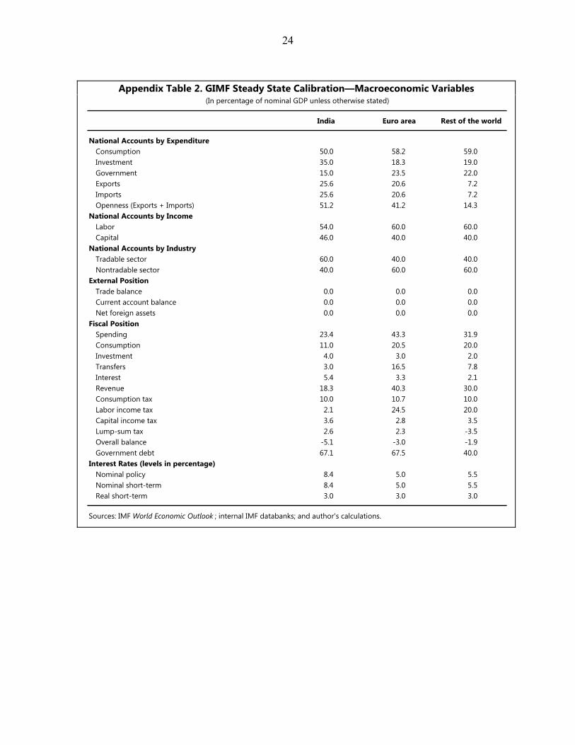
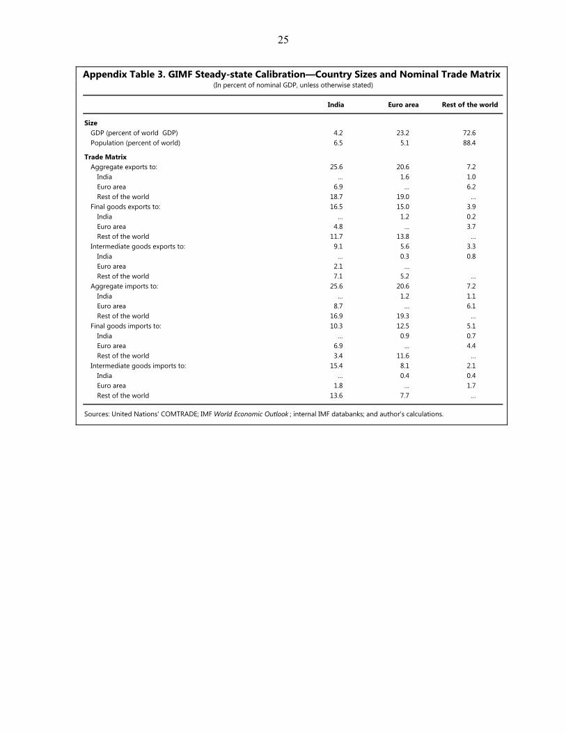
All the results are gauged relative to the steady state (see Appendix Table 2). Steady-state GDP decomposition, the matrix of bilateral trade flows, and debt ratios are based on recent historical averages (2007–11) from the United Nations’ COMTRADE, the IMF World Economic Outlook, and internal IMF databanks. The steady-state world technology growth rate is fixed at 1.5 percent per annum and the world population growth rate at 1 percent per annum. The world long-run real interest rate is set at 3 percent per annum. In the steady state, India accounts for 4.2 percent of world nominal GDP and 6.5 percent of world population; the euro area represents 23.2 percent of world output and 5.1 percent of the total population. With regard to GDP components, the steady-state consumption-to-GDP ratio is relatively lower in India but the investment rate is almost twice that of the euro area. Government expenditure is relatively lower in India—15 percent compared with 23 percent in other blocks. Net holdings of foreign assets are assumed to be 0, implying that no region could run a persistent trade surplus. Accordingly, exports and imports are equalized for all the regions in the steady state. India is distinctively more open than the euro area. Labor share in income is 54 percent for India, slightly lower than that for other regions where the average is about 60 percent. The equilibrium policy rate for India is 8.4 percent, reflecting the assumptions of

4 To determine the degree of pro-cyclicality of fiscal policy, the following regression Δ has been estimated for India and the euro area. denotes real public spending , represents real output, and measures the extent of pro ( 0 ) or counter ( 0 ) cyclical policy. The estimated coefficient  turns out to be higher (0.13) for the euro area compared with only 0.02 for India. Accordingly, India is assumed to be less pro-cyclical than the euro area thereby a lower value for the parameter .

8

3 percent of global real short-term rates and the above-mentioned inflation target. The steady-state fiscal situation in India is as follows: the overall deficit is 5 percent of GDP and the public debt-to-GDP ratio is 67 percent (close to the medium-term goal of the government). Government consumption accounts for more than half of total primary spending. Similarly, the consumption tax is the principal source of revenue. It is worth noting that India’s actual figures are slightly different from the steady-state values. This is because steady-state values result from the optimization of the model given all other parameters. Moreover, in GIMF the sizes of the absolute magnitudes are less critical than the structural parameters and macroeconomic ratios.

III. CONSOLIDATION STRATEGIES

The design and implementation of the consolidation plan (such as instrument choice, timing, and auxiliary measures) are country- and circumstance-specific and are crucial for the net growth effect (see Botman and Honjo, 2006; Botman et al., 2009; Berkmen, 2011; Clinton et al., 2011; and Taylor et al., 2013).

The composition of instruments has a critical impact on growth. Achieving consolidation solely through one instrument, such as higher taxes or lower expenditure, would require substantial changes to tax or spending levels, and could be extremely costly in terms of welfare and equity. For instance, cutting only transfers or raising only the consumption tax would have a significant impact on poor households, while curtailing investment would have a lasting effect on output. Therefore, a successful consolidation package should be a blend of expenditure and revenue measures to share the burden across instruments and groups.

The particular plans laid out here follow the spirit of the Thirteenth Finance Commission, the Kelkar et al. (2012) report, and the finance minister’s 2012 roadmap. The consolidation strategy targets the elimination of the steady-state deficit (5 percent) over five years. This assumption is illustrative because the relationship between the size of the adjustment and the size of the response is approximately linear.

Three fiscal adjustment packages, comparable in terms of deficit reduction, are assessed: benchmark (lowering unproductive expenditure and strengthening consumption tax revenue); growth-friendly (reducing unproductive outlays, improving consumption tax revenue, and increasing public investment); and social-friendly (bringing down unproductive spending, improving the efficiency of the consumption tax, and increasing social spending for the poorest) scenarios (Table 1).

9

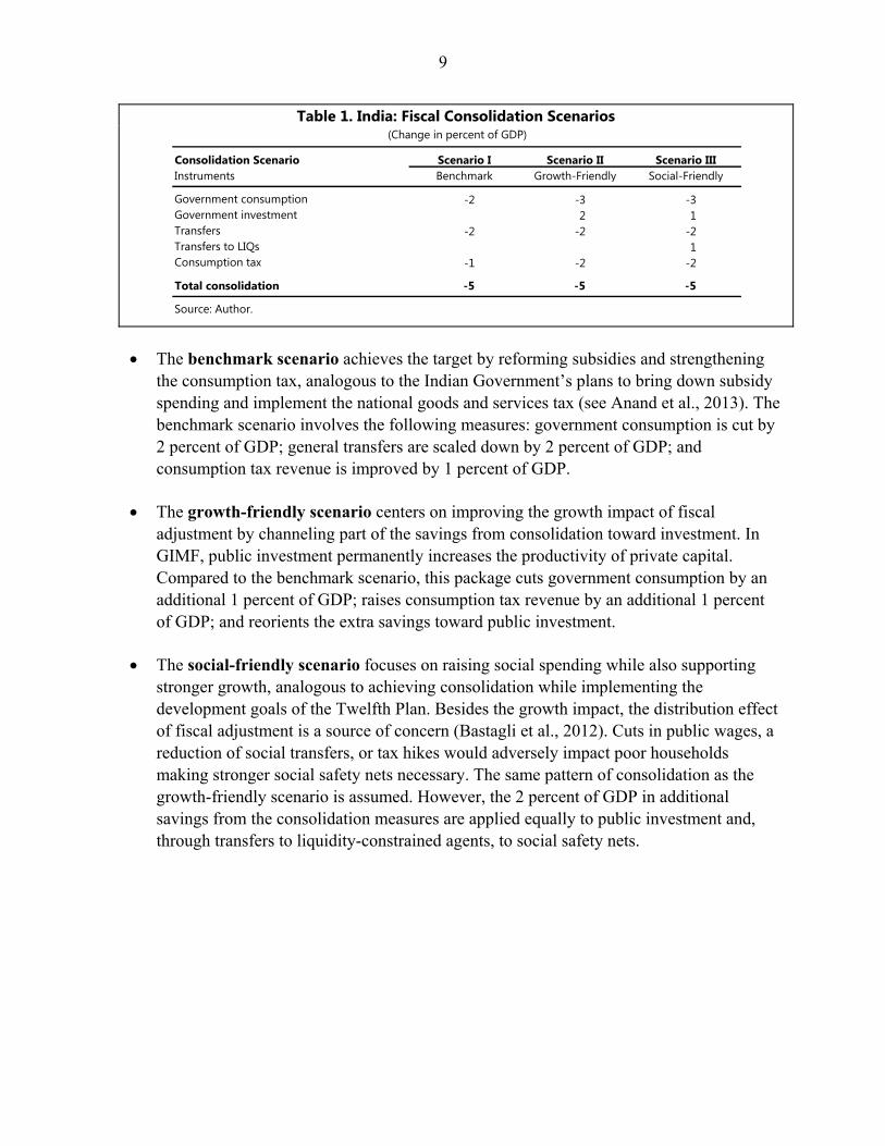
Table 1. India: Fiscal Consolidation Scenarios

The benchmark scenario achieves the target by reforming subsidies and strengthening

the consumption tax, analogous to the Indian Government’s plans to bring down subsidy spending and implement the national goods and services tax (see Anand et al., 2013). The benchmark scenario involves the following measures: government consumption is cut by 2 percent of GDP; general transfers are scaled down by 2 percent of GDP; and consumption tax revenue is improved by 1 percent of GDP.

The growth-friendly scenario centers on improving the growth impact of fiscal

adjustment by channeling part of the savings from consolidation toward investment. In GIMF, public investment permanently increases the productivity of private capital. Compared to the benchmark scenario, this package cuts government consumption by an additional 1 percent of GDP; raises consumption tax revenue by an additional 1 percent of GDP; and reorients the extra savings toward public investment.

The social-friendly scenario focuses on raising social spending while also supporting

stronger growth, analogous to achieving consolidation while implementing the development goals of the Twelfth Plan. Besides the growth impact, the distribution effect of fiscal adjustment is a source of concern (Bastagli et al., 2012). Cuts in public wages, a reduction of social transfers, or tax hikes would adversely impact poor households making stronger social safety nets necessary. The same pattern of consolidation as the growth-friendly scenario is assumed. However, the 2 percent of GDP in additional savings from the consolidation measures are applied equally to public investment and, through transfers to liquidity-constrained agents, to social safety nets.

Consolidation Scenario Scenario I Scenario II Scenario IIIInstruments Benchmark Growth-Friendly Social-Friendly

Government consumption -2 -3 -3Government investment 2 1Transfers -2 -2 -2Transfers to LIQs 1Consumption tax -1 -2 -2

Total consolidation -5 -5 -5

Source: Author.

(Change in percent of GDP)

10

IV. POLICY SIMULATIONS

A. Baseline Simulations

Fiscal multipliers

The fiscal multiplier is the best measure to analyze the effects of various fiscal tools in isolation. In the discussion below, a standardized shock of 1 percent of GDP in the direction of consolidation is assumed for each instrument (i.e., a stimulus via revenue or expenditure measures of 1 percent of GDP). The multiplier for each year is obtained as the change in real GDP resulting from the shock.

Short-run multipliers are calculated by looking at the immediate impact of the fiscal stimulus in the current year. The multipliers for government consumption and investment are the highest, 1 and 1.4 respectively (see Table 2). The relatively high multiplier for government investment in India reflects the higher initial investment rates; the contribution of investment to output growth is larger when investment is a larger share of GDP. Transfers produce a smaller multiplier of only 0.2 because of the high proportion of liquidity-constrained households. The multiplier for consumption tax is estimated at 0.4.

Over a 10-year horizon, multipliers vary significantly. All other things being equal, a public investment cut has the most detrimental impact on growth. A decline in investment immediately produces a drop in global demand and undermines future production capacity. Multipliers are lower for a government consumption cut and consumption tax hike. Reduced transfers have a lower short-term growth cost and produce significant permanent gain in GDP in the medium term (Table 2).

In Table 3, India’s fiscal multipliers are compared with the relevant literature. The estimated multipliers are consistent with the literature based on DSGE and vector autoregression (VAR) frameworks (see Baunsgaard et al., 2013; and Jain and Kumar, 2013). Based on structural VAR estimates, Jain and Kumar (2013) find that the multiplier of government spending equals 0.6, lower than the average across fiscal instruments discussed above which is about 0.9. They also document that the multiplier for capital outlays is well above one implying that public investment in India is more growth inducing than current expenditure as mentioned above. Furthermore, the model-generated multipliers are broadly in-line with the worldwide estimates. Baunsgaard et al. (2013) reviewed a total of 37 studies including both DSGE and VAR approaches. The average first-year multiplier in the existing literature is between 0.7 and 0.9 for spending measures and between 0.2 and 0.3 for revenue measures.

11

Table 2. India: Impact of Fiscal Consolidation on Real GDP by Instrument

Table 3. First-Year Fiscal Multipliers: India and Selected Regions

Fiscal consolidation

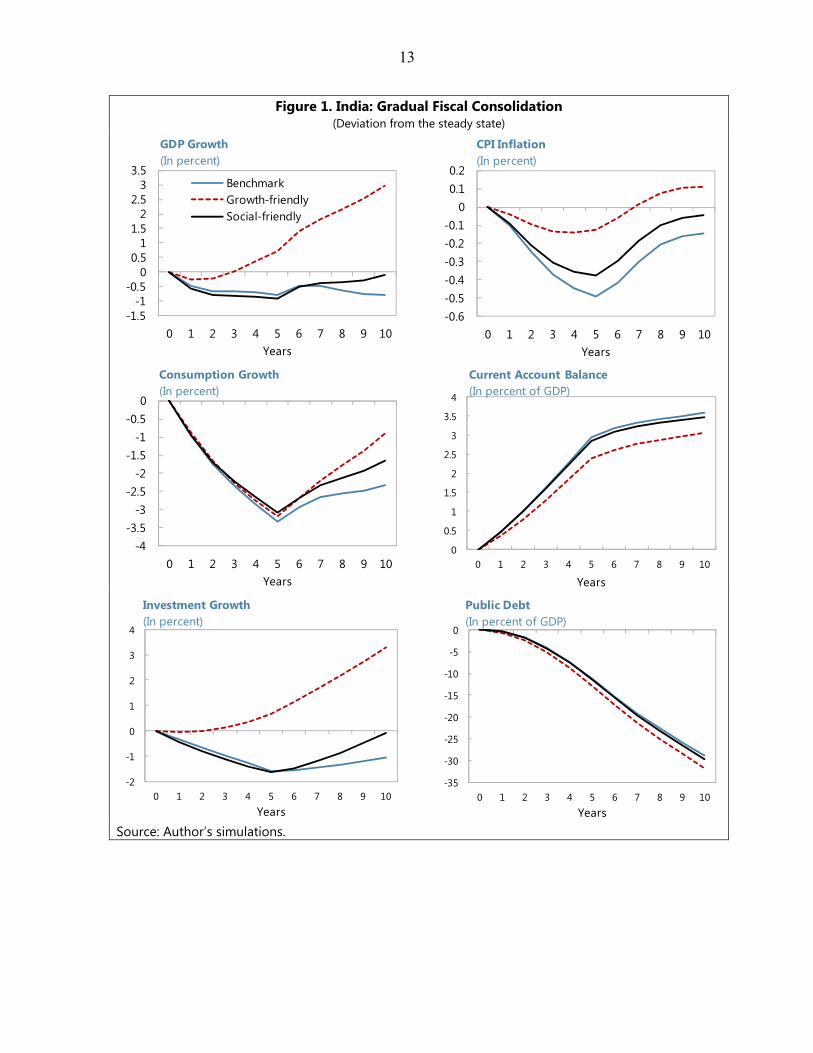
The baseline analysis assumes that the consolidation plan is carried out gradually and uniformly over five years (see Figure 1). All scenarios reduce the steady-state debt ratio by almost 30 percentage points of GDP relative to the steady state over 10 years, though output diverges significantly. It is worthwhile noting that the debt ratio does not decrease one-for-one with fiscal tightening.

The reason is that fiscal tightening reduces GDP; lower GDP in turn reduces the denominator of the debt ratio and also partly offsets the debt reduction in the numerator. Also, there is a stabilization rule in the fiscal sector that prevents a volatile government debt ratio. It is assumed that revenue or expenditure would adjust to stabilize the government surplus-to-GDP ratio at a long-run level. This leads to a slow mean reversion of debt.

Owing to stronger investment, the growth-friendly strategy produces the highest growth path with the short-term contraction offset. In the long run, output growth is

Government Government Government Government Consumption Consumption Transfers Transfers to LIQs Investment Tax

Year 1 1.0 0.2 0.2 1.4 0.4Year 2 0.2 0.0 -0.1 0.5 0.2Year 3 -0.1 -0.2 -0.4 0.3 0.0Year 4 -0.1 -0.2 -0.4 0.4 0.0Year 5 0.1 -0.2 -0.4 0.8 0.1Year 6 0.2 -0.2 -0.4 1.1 0.1Year 7 0.2 -0.1 -0.4 1.3 0.1Year 8 0.1 -0.2 -0.5 1.3 0.1Year 9 0.0 -0.2 -0.5 1.4 0.1Year 10 0.0 -0.2 -0.5 1.5 0.0

Source: Author's calculations.Note: Multipliers reported here reflect the real GDP response (in percent) to a 1 percent fiscal shock.

(Percent Deviation from the Steady State)

DSGE VAR DSGE VARIndia 0.9 (1) 0.6 (2) 0.4 (2) 0.4 (2)

United States 0.7 1.0 0.3 0.7European union 0.6 0.8 0.1 -0.3World 0.7 0.9 0.3 0.2

Sources: Based on Baunsgaard et al. (2013); Jain and Kumar (2013); and author's simulations.(1) Average across instruments; (2) India's VAR estimates are based on Jain and Kumar (2013).Note: VAR denotes summary statistics from linear vector autoregressive models, and DSGE denotes results from dynamic stochastic general equilibrium models.

GovernmentSpending Revenue

Government

12

almost 3 percent higher than the steady state. Because of the relatively higher growth, the reduction in the debt-to-GDP ratio is relatively faster under the growth-friendly scenario. There is no overheating, as strong investment means capacity constraints do not bind, so inflation remains broadly unchanged. Following the logic of twin deficits, a reduction of the fiscal balance translates into an improvement of the current account balance of about 3 percent compared with the steady state in the long run.

In the social-friendly consolidation, the adverse impacts of a government consumption cut and a consumption tax hike accumulate over time. Output growth falls by about 1 percent relative to the steady state and does not recover, as consumption and investment growth remain negative. Sluggish growth is accompanied by lower inflation of almost 0.5 percent relative to the steady state. In the scenario, the bulk of capital goods is imported. Under the social-friendly adjustments, the current account balance improves quickly as a result of lower imports (investment-related) compared to the growth-friendly strategy.

The outcome under the benchmark scenario is similar to that observed under the social-friendly consolidation. Relative to the steady state, the growth rates of output, consumption, and investment contract and remain in negative territory. The decline of inflation is more pronounced in the benchmark case. As is the case under the social-friendly scenario, the current account balance improves quickly.

These various simulations indicate that, in the medium term, policymakers face a trade-off between higher growth (economic efficiency) and welfare for poorer households (distribution effect). The growth-friendly scenario promotes efficient public investment that leads to stronger growth which is not necessarily inclusive, whereas the social-friendly scenario produces lower growth but promotes more efficiently targeted social spending to mitigate the short-run adverse impact of public sector contraction.

B. Additional Simulations

Magnitude and timetable

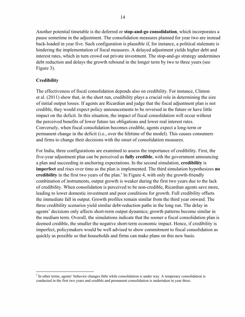
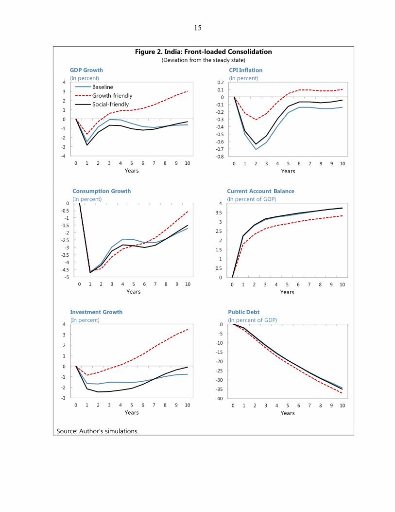
This section assesses how shifting the balance of consolidation efforts over time affects outcomes. Under the front-loaded consolidation, all the necessary adjustments are implemented in the first year. Compared with the gradual strategy, the profiles of key macroeconomic variables are very similar, but diverge in terms of timing and magnitude. A larger and immediate consolidation lowers the debt ratio by an additional 5 percent of GDP in the tenth year but the output loss is three times higher (see Figure 2). As previously, the medium-term output recovery only materializes in the growth-friendly scenario. In general, an up-front adjustment pares down the debt ratio further and firms up market sentiment; however, the short-term output loss is much greater and recovery comes only in the medium term. From the policymakers’ perspective, the confidence-building benefits of a front-loaded consolidation would need to be balanced with the cost to growth in the short run.

13

Figure 1. India: Gradual Fiscal Consolidation (Deviation from the steady state)

Source: Author’s simulations.

-1.5-1

-0.50

0.51

1.52

2.53

3.5

0 1 2 3 4 5 6 7 8 9 10Years

BenchmarkGrowth-friendlySocial-friendly

GDP Growth (In percent)

-0.6-0.5-0.4-0.3-0.2-0.1

00.10.2

0 1 2 3 4 5 6 7 8 9 10Years

CPI Inflation (In percent)

-4-3.5

-3-2.5

-2-1.5

-1-0.5

0

0 1 2 3 4 5 6 7 8 9 10Years

Consumption Growth (In percent)

0

0.5

1

1.5

2

2.5

3

3.5

4

0 1 2 3 4 5 6 7 8 9 10

Years

Current Account Balance (In percent of GDP)

-2

-1

0

1

2

3

4

0 1 2 3 4 5 6 7 8 9 10Years

Investment Growth (In percent)

-35

-30

-25

-20

-15

-10

-5

0

0 1 2 3 4 5 6 7 8 9 10Years

Public Debt (In percent of GDP)

14

Another potential timetable is the deferred or stop-and-go consolidation, which incorporates a pause sometime in the adjustment. The consolidation measures planned for year two are instead back-loaded in year five. Such configuration is plausible if, for instance, a political stalemate is hindering the implementation of fiscal measures. A delayed adjustment yields higher debt and interest rates, which in turn crowd out private investment. The stop-and-go strategy undermines debt reduction and delays the growth rebound in the longer term by two to three years (see Figure 3). Credibility

The effectiveness of fiscal consolidation depends also on credibility. For instance, Clinton et al. (2011) show that, in the short run, credibility plays a crucial role in determining the size of initial output losses. If agents are Ricardian and judge that the fiscal adjustment plan is not credible, they would expect policy announcements to be reversed in the future or have little impact on the deficit. In this situation, the impact of fiscal consolidation will occur without the perceived benefits of lower future tax obligations and lower real interest rates. Conversely, when fiscal consolidation becomes credible, agents expect a long-term or permanent change in the deficit (i.e., over the lifetime of the model). This causes consumers and firms to change their decisions with the onset of consolidation measures.

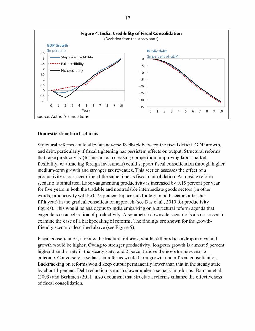
For India, three configurations are examined to assess the importance of credibility. First, the five-year adjustment plan can be perceived as fully credible, with the government announcing a plan and succeeding in anchoring expectations. In the second simulation, credibility is imperfect and rises over time as the plan is implemented. The third simulation hypothesizes no credibility in the first two years of the plan.5 In Figure 4, with only the growth-friendly combination of instruments, output growth is weaker during the first two years due to the lack of credibility. When consolidation is perceived to be non-credible, Ricardian agents save more, leading to lower domestic investment and poor conditions for growth. Full credibility offsets the immediate fall in output. Growth profiles remain similar from the third year onward. The three credibility scenarios yield similar debt-reduction paths in the long run. The delay in agents’ decisions only affects short-term output dynamics; growth patterns become similar in the medium term. Overall, the simulations indicate that the sooner a fiscal consolidation plan is deemed credible, the smaller the negative short-term economic impact. Hence, if credibility is imperfect, policymakers would be well advised to show commitment to fiscal consolidation as quickly as possible so that households and firms can make plans on this new basis.

5 In other terms, agents’ behavior changes little while consolidation is under way. A temporary consolidation is conducted in the first two years and credible and permanent consolidation is undertaken in year three.

15

Figure 2. India: Front-loaded Consolidation (Deviation from the steady state)

Source: Author’s simulations.

-4

-3

-2

-1

0

1

2

3

4

0 1 2 3 4 5 6 7 8 9 10Years

BaselineGrowth-friendlySocial-friendly

GDP Growth (In percent)

-0.8-0.7-0.6-0.5-0.4-0.3-0.2-0.1

00.10.2

0 1 2 3 4 5 6 7 8 9 10Years

CPI Inflation (In percent)

-5-4.5

-4-3.5

-3-2.5

-2-1.5

-1-0.5

0

0 1 2 3 4 5 6 7 8 9 10Years

Consumption Growth(In percent)

0

0.5

1

1.5

2

2.5

3

3.5

4

0 1 2 3 4 5 6 7 8 9 10Years

Current Account Balance (In percent of GDP)

-3

-2

-1

0

1

2

3

4

0 1 2 3 4 5 6 7 8 9 10Years

Investment Growth (In percent)

-40

-35

-30

-25

-20

-15

-10

-5

0

0 1 2 3 4 5 6 7 8 9 10Years

Public Debt (In percent of GDP)

16

Figure 3. India: Stop-and-Go Fiscal Consolidation (Deviation from the steady state)

Source: Author’s simulations.

-2

-1.5

-1

-0.5

0

0.5

1

1.5

2

0 1 2 3 4 5 6 7 8 9 10Years

BaselineGrowth-friendlySocial-friendly

GDP Growth (In percent)

-0.6

-0.5

-0.4

-0.3

-0.2

-0.1

0

0.1

0.2

0 1 2 3 4 5 6 7 8 9 10Years

CPI inflation (In percent)

-4.5

-4

-3.5

-3

-2.5

-2

-1.5

-1

-0.5

0

0 1 2 3 4 5 6 7 8 9 10Years

Consumption Growth (In percent)

0

0.5

1

1.5

2

2.5

3

3.5

4

0 1 2 3 4 5 6 7 8 9 10Years

Current Account Balance (In percent of GDP)

-2

-1.5

-1

-0.5

0

0.5

1

1.5

2

2.5

0 1 2 3 4 5 6 7 8 9 10Years

Investment Growth (In percent)

-35

-30

-25

-20

-15

-10

-5

0

0 1 2 3 4 5 6 7 8 9 10Years

Public Debt (In percent of GDP)

17

Figure 4. India: Credibility of Fiscal Consolidation (Deviation from the steady state)

Source: Author’s simulations.

Domestic structural reforms

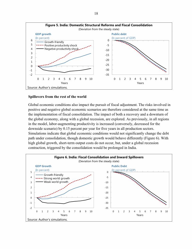
Structural reforms could alleviate adverse feedback between the fiscal deficit, GDP growth, and debt, particularly if fiscal tightening has persistent effects on output. Structural reforms that raise productivity (for instance, increasing competition, improving labor market flexibility, or attracting foreign investment) could support fiscal consolidation through higher medium-term growth and stronger tax revenues. This section assesses the effect of a productivity shock occurring at the same time as fiscal consolidation. An upside reform scenario is simulated. Labor-augmenting productivity is increased by 0.15 percent per year for five years in both the tradable and nontradable intermediate goods sectors (in other words, productivity will be 0.75 percent higher indefinitely in both sectors after the fifth year) in the gradual consolidation approach (see Das et al., 2010 for productivity figures). This would be analogous to India embarking on a structural reform agenda that engenders an acceleration of productivity. A symmetric downside scenario is also assessed to examine the case of a backpedaling of reforms. The findings are shown for the growth-friendly scenario described above (see Figure 5).

Fiscal consolidation, along with structural reforms, would still produce a drop in debt and growth would be higher. Owing to stronger productivity, long-run growth is almost 5 percent higher than the rate in the steady state, and 2 percent above the no-reforms scenario outcome. Conversely, a setback in reforms would harm growth under fiscal consolidation. Backtracking on reforms would keep output permanently lower than that in the steady state by about 1 percent. Debt reduction is much slower under a setback in reforms. Botman et al. (2009) and Berkmen (2011) also document that structural reforms enhance the effectiveness of fiscal consolidation.

-1

-0.5

0

0.5

1

1.5

2

2.5

3

3.5

0 1 2 3 4 5 6 7 8 9 10

Years

Stepwise credibility

Full credibility

No credibility

GDP Growth (In percent)

-35

-30

-25

-20

-15

-10

-5

0

0 1 2 3 4 5 6 7 8 9 10

Public debt (In percent of GDP)

18

Figure 5. India: Domestic Structural Reforms and Fiscal Consolidation (Deviation from the steady state)

Source: Author’s simulations. Spillovers from the rest of the world

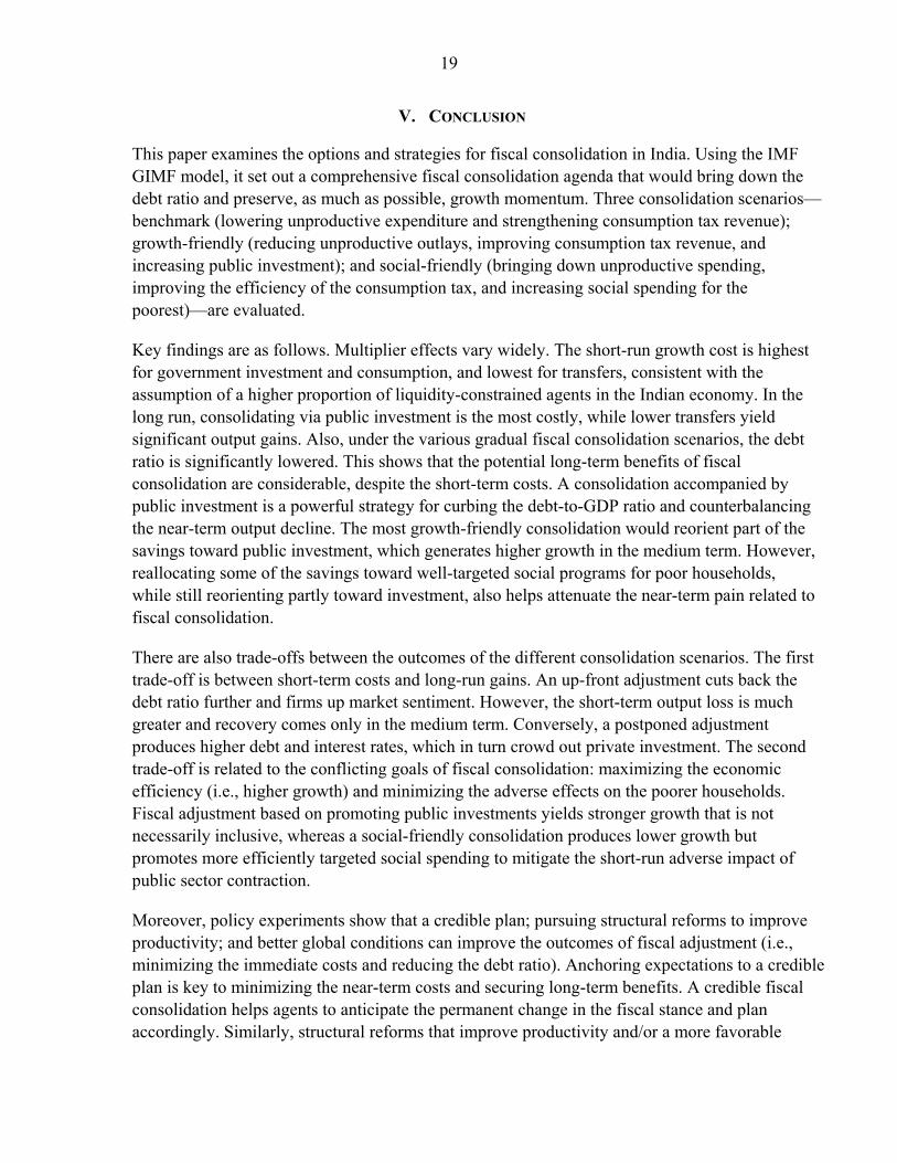
Global economic conditions also impact the pursuit of fiscal adjustment. The risks involved in positive and negative global economic scenarios are therefore considered at the same time as the implementation of fiscal consolidation. The impact of both a recovery and a downturn of the global economy, along with a global recession, are explored. As previously, in all regions in the model, labor-augmenting productivity is increased (conversely, decreased for the downside scenario) by 0.15 percent per year for five years in all production sectors. Simulations indicate that global economic conditions would not significantly change the debt path under consolidation, though domestic growth would behave differently (Figure 6). With high global growth, short-term output costs do not occur, but, under a global recession contraction, triggered by the consolidation would be prolonged in India.

Figure 6. India: Fiscal Consolidation and Inward Spillovers (Deviation from the steady state)

Source: Author’s simulations.

-2-10123456

0 1 2 3 4 5 6 7 8 9 10Years

Growth-friendlyPositive productivity shockNegative productivity shock

GDP growth (In percent)

-35

-30

-25

-20

-15

-10

-5

0

0 1 2 3 4 5 6 7 8 9 10Years

Public debt (In percent of GDP)

-2

-1

0

1

2

3

4

5

0 1 2 3 4 5 6 7 8 9 10Years

Growth-friendlyStrong world growthWeak world growth

GDP Growth (In percent)

-35

-30

-25

-20

-15

-10

-5

0

0 1 2 3 4 5 6 7 8 9 10Years

Public Debt (In percent of GDP)

19

V. CONCLUSION

This paper examines the options and strategies for fiscal consolidation in India. Using the IMF GIMF model, it set out a comprehensive fiscal consolidation agenda that would bring down the debt ratio and preserve, as much as possible, growth momentum. Three consolidation scenarios— benchmark (lowering unproductive expenditure and strengthening consumption tax revenue); growth-friendly (reducing unproductive outlays, improving consumption tax revenue, and increasing public investment); and social-friendly (bringing down unproductive spending, improving the efficiency of the consumption tax, and increasing social spending for the poorest)—are evaluated.

Key findings are as follows. Multiplier effects vary widely. The short-run growth cost is highest for government investment and consumption, and lowest for transfers, consistent with the assumption of a higher proportion of liquidity-constrained agents in the Indian economy. In the long run, consolidating via public investment is the most costly, while lower transfers yield significant output gains. Also, under the various gradual fiscal consolidation scenarios, the debt ratio is significantly lowered. This shows that the potential long-term benefits of fiscal consolidation are considerable, despite the short-term costs. A consolidation accompanied by public investment is a powerful strategy for curbing the debt-to-GDP ratio and counterbalancing the near-term output decline. The most growth-friendly consolidation would reorient part of the savings toward public investment, which generates higher growth in the medium term. However, reallocating some of the savings toward well-targeted social programs for poor households, while still reorienting partly toward investment, also helps attenuate the near-term pain related to fiscal consolidation.

There are also trade-offs between the outcomes of the different consolidation scenarios. The first trade-off is between short-term costs and long-run gains. An up-front adjustment cuts back the debt ratio further and firms up market sentiment. However, the short-term output loss is much greater and recovery comes only in the medium term. Conversely, a postponed adjustment produces higher debt and interest rates, which in turn crowd out private investment. The second trade-off is related to the conflicting goals of fiscal consolidation: maximizing the economic efficiency (i.e., higher growth) and minimizing the adverse effects on the poorer households. Fiscal adjustment based on promoting public investments yields stronger growth that is not necessarily inclusive, whereas a social-friendly consolidation produces lower growth but promotes more efficiently targeted social spending to mitigate the short-run adverse impact of public sector contraction.

Moreover, policy experiments show that a credible plan; pursuing structural reforms to improve productivity; and better global conditions can improve the outcomes of fiscal adjustment (i.e., minimizing the immediate costs and reducing the debt ratio). Anchoring expectations to a credible plan is key to minimizing the near-term costs and securing long-term benefits. A credible fiscal consolidation helps agents to anticipate the permanent change in the fiscal stance and plan accordingly. Similarly, structural reforms that improve productivity and/or a more favorable

20

external environment enhance the effectiveness of fiscal consolidation by mitigating the near-term output loss and producing higher gains in the long run.

In order to enhance savings while limiting the negative effects on growth, India could take several measures including reducing unproductive government spending, especially by better targeting fuel subsidies, and increasing the buoyancy of the consumption tax as the growth effects of such measures would be relatively contained. The potential negative effects of a consolidation based on these instruments could also be contained by reorienting some savings toward greater infrastructure investment and/or social safety nets, as envisaged under the Twelfth Plan.

21

REFERENCES

Anand, R., D. Coady, A. Mohommad, V. Thakoor, and J. Walsh, 2013, “The Fiscal and Welfare Impact of Reforming Fuel Subsidies in India,” IMF Working Paper (forthcoming; Washington: International Monetary Fund).

Bastagli, F., D. Coady, and S. Gupta, 2012, “Income Inequality and Fiscal Policy,” IMF Staff Discussion Note 12/286 (Washington: International Monetary Fund).

Baum, A., M. Poplawski-Ribeiro, and A. Weber, 2012, “Fiscal Multipliers and the State of the Economy,” IMF Working Paper 12/286 (Washington: International Monetary Fund).

Baunsgaard, T., M. Mineshima, M. Poplawski-Ribeiro, and A. Weber, 2013, “Fiscal Multipliers,” in “Post-Crisis Fiscal Policy”, C. Cottarelli, P. Gerson, and A. Senhadji, eds. (forthcoming; Washington: International Monetary Fund).

Berkmen, S. P., 2011, “The Impact of Fiscal Consolidation and Structural Reforms on Growth in Japan,” IMF Working Paper 11/13 (Washington: International Monetary Fund).

Bernanke, B., M. Gertler, and S.Gilchrist, 1999,”The Financial Accelerator in a Quantitative Business Cycle Framework,” in John Taylor and Michael Woodford, eds., Handbook of Macroeconomics. Amsterdam: North Holland.

Blanchard, O. and D. Leigh, 2013, “Growth Forecast Errors and Fiscal Multipliers,” IMF Working Paper 13/1 (Washington: International Monetary Fund).

Botman, D., and K. Honjo, 2006, “Options for Fiscal Consolidation in the United Kingdom,” IMF Working Paper 06/89 (Washington: International Monetary Fund).

_________, H. Edison, and P. N’Diaye, 2009, “Strategies for Fiscal Consolidation in Japan,” Japan and the World Economy, Vol. 21, Issue 2 (March), pp. 151–60.

Clinton, K., M. Kumhof, D. Laxton, and S. Mursula, 2011, “Deficit Reduction: Short-Term Pain for Long-Term Gain,” European Economic Review, Vol. 55, Issue 1 (January), pp. 118–39.

Corsetti, G., K. Kuester, M. André, and G. J. Müller, 2010, “Debt Consolidation and Fiscal Stabilization of Deep Recessions,” American Economic Review, Vol. 100, Issue 2 (May), pp. 41–45.

Das, D., A. Erumban, , S. Aggarwal, and D. Wadhwa, 2010, “Total Factor Productivity Growth in India in the Reform Period: A Disaggregated Sectoral Analysis.” Available via the Internet: www.worldklems.net/conferences/worldklems2010_das_wadhwa.pdf

Erceg, C. J. and J. Lindé, 2013, “Fiscal Consolidation in a Currency Union: Spending Cuts vs. Tax Hikes,” Journal of Economic Dynamics and Control, Vol. 37, Issue 2 (February), pp. 422–45.

22

Finance Commission of India 2009 (December), “Finance Commission Report of the Thirteenth Finance Commission (2010–15). ” Available via the Internet: http://fincomindia.nic.in/writereaddata/html_en_files/oldcommission_html/fincom13/tfc/13fcreng.pdf

Government of India, 2010–12, “Union Budget.” Available via the Internet: http://indiabudget.nic.in/

Jain, R., and P. Kumar, 2013, “Size of Government Expenditure Multipliers in India: A Structural VAR Analysis,” RBI Working Paper (forthcoming; Mumbai: Reserve Bank of India).

Kelkar, V. L., I. Rajaraman, and S. Misra, 2012, “Report of the Committee on Roadmap for Fiscal Consolidation” (Government of India: Ministry of Finance). Available via the Internet: finmin.nic.in/reports/Kelkar_Committee_Report.pdf

Kumhof, M., D. Muir, S. Mursula, and D. Laxton, 2010, “The Global Integrated Monetary and Fiscal Model (GIMF) ─Theoretical Structure,” IMF Working Paper 10/34 (Washington: International Monetary Fund).

Ministry of Finance of India, 2012 (October), “Statement of the Union Finance Minister Shri P. Chidambaram on Fiscal Roadmap and Consolidation.” Available via the Internet: http://pib.nic.in/newsite/erelease.aspx?relid=88669

Mundle, S., N.R. Bhanumurthy, and S. Das, 2011, “Fiscal Consolidation with High Growth: A Policy Simulation Model for India,” Economic Modelling, Vol. 28, Issue 6 (November), pp. 2657–68.

Taylor, J., J., Cogan, V. Wieland, and M. Wolters, 2013, “Fiscal Consolidation Strategy,” Journal of Economic Dynamics and Control, Vol. 37, Issue 2 (February), pp. 404–21.

23

APPENDIX

Appendix Table 1. GIMF Dynamic Model Calibration

India Euro area Rest of the world

Long-Run Growth Rates and Interest RatesWorld technology growth 1.5 1.5 1.5World population growth 1.0 1.0 1.0Steady state inflation rate 5.5 2.0 2.5Long-run real interest rate 3.0 3.0 3.0

Utility FunctionsAverage planning horizon in years 20.0 20.0 20.0Average remaining working life in years 20.0 20.0 20.0Intertemporal elasticity of substitution 0.3 0.3 0.3Degree of habit persistence 0.4 0.4 0.4Labor supply elasticity 0.5 0.5 0.5Share of liquidity-constrained agents 0.5 0.3 0.4

Production Parameters (elasticity of substitution between)Capital and labor 1.0 1.0 1.0Domestic and foreign traded goods 1.5 1.5 1.5Foreign traded goods 1.5 1.5 1.5Tradable and nontradable goods 0.5 0.5 0.5

Price and Wage Markups (percentage of marginal cost)Nontradables manufacturing 10.0 10.0 10.0Tradables manufacturing 10.0 10.0 10.0Union wage setting 10.0 10.0 10.0Retail sector 5.0 5.0 5.0Consumption goods production 5.0 5.0 5.0Investment goods production 5.0 5.0 5.0Final imports 2.5 2.5 2.5Intermediate imports 2.5 2.5 2.5

Nominal RigiditiesReal wage 30.0 47.0 40.0Consumption price 40.0 60.0 40.0Investment price 40.0 60.0 40.0Nontradables price 40.0 60.0 40.0Tradables price 40.0 60.0 40.0Price of imports of final goods (DM) 4.0 20.0 40.0Price of imports of intermediate goods (TM) 4.0 20.0 40.0

Real Adjustment CostsLabor demand 1.0 1.0 1.0Consumption 2.0 2.0 2.0Investment 1.0 1.0 1.0Imports of consumption goods 1.0 1.0 1.0Imports of investment goods 1.0 1.0 1.0Imports of tradables goods 1.0 1.0 1.0

Depreciation RateBusiness capital stock 0.1 0.1 0.1Public capital stock 0.0 0.0 0.0Public durables stock 0.0 0.0 0.0

Monetary Policy and Fiscal Policy Parametersδi 0.3 0.3 0.3δπ 1.0 1.5 1.2Inflation target 5.5 2.0 2.5dgdp 0.3 0.5 0.3

Sources: Kumhof et al. 2010; and author's calculations.

Parameters

24

Appendix Table 2. GIMF Steady State Calibration—Macroeconomic Variables

India Euro area Rest of the world

National Accounts by ExpenditureConsumption 50.0 58.2 59.0Investment 35.0 18.3 19.0Government 15.0 23.5 22.0Exports 25.6 20.6 7.2Imports 25.6 20.6 7.2Openness (Exports + Imports) 51.2 41.2 14.3

National Accounts by IncomeLabor 54.0 60.0 60.0Capital 46.0 40.0 40.0

National Accounts by IndustryTradable sector 60.0 40.0 40.0Nontradable sector 40.0 60.0 60.0

External PositionTrade balance 0.0 0.0 0.0Current account balance 0.0 0.0 0.0Net foreign assets 0.0 0.0 0.0

Fiscal PositionSpending 23.4 43.3 31.9Consumption 11.0 20.5 20.0Investment 4.0 3.0 2.0Transfers 3.0 16.5 7.8Interest 5.4 3.3 2.1Revenue 18.3 40.3 30.0Consumption tax 10.0 10.7 10.0Labor income tax 2.1 24.5 20.0Capital income tax 3.6 2.8 3.5Lump-sum tax 2.6 2.3 -3.5Overall balance -5.1 -3.0 -1.9Government debt 67.1 67.5 40.0

Interest Rates (levels in percentage)Nominal policy 8.4 5.0 5.5Nominal short-term 8.4 5.0 5.5Real short-term 3.0 3.0 3.0

Sources: IMF World Economic Outlook ; internal IMF databanks; and author's calculations.

(In percentage of nominal GDP unless otherwise stated)

25

Appendix Table 3. GIMF Steady-state Calibration—Country Sizes and Nominal Trade Matrix

India Euro area Rest of the world

SizeGDP (percent of world GDP) 4.2 23.2 72.6Population (percent of world) 6.5 5.1 88.4

Trade MatrixAggregate exports to: 25.6 20.6 7.2

India … 1.6 1.0Euro area 6.9 … 6.2Rest of the world 18.7 19.0 …

Final goods exports to: 16.5 15.0 3.9India … 1.2 0.2Euro area 4.8 … 3.7Rest of the world 11.7 13.8 …

Intermediate goods exports to: 9.1 5.6 3.3India … 0.3 0.8Euro area 2.1 …Rest of the world 7.1 5.2 …

Aggregate imports to: 25.6 20.6 7.2India … 1.2 1.1Euro area 8.7 … 6.1Rest of the world 16.9 19.3 …

Final goods imports to: 10.3 12.5 5.1India … 0.9 0.7Euro area 6.9 … 4.4Rest of the world 3.4 11.6 …

Intermediate goods imports to: 15.4 8.1 2.1India … 0.4 0.4Euro area 1.8 … 1.7Rest of the world 13.6 7.7 …

Sources: United Nations' COMTRADE; IMF World Economic Outlook ; internal IMF databanks; and author's calculations.

(In percent of nominal GDP, unless otherwise stated)