Options Off-policy learning with options and recognizersold.sztaki.hu/~szcsaba/research/AAAI10_Tutorial/tutorial01-splitshow.pdf · ¥ G i ven s ampl es from pol ... The update to

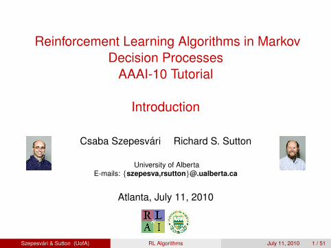
Reinforcement Learning Algorithms in MarkovDecision Processes

AAAI-10 Tutorial

Introduction

Csaba Szepesvari Richard S. Sutton

University of AlbertaE-mails: {szepesva,rsutton}@.ualberta.ca

Atlanta, July 11, 2010

Szepesvari & Sutton (UofA) RL Algorithms July 11, 2010 1 / 51

Contributions! !"# !"$ %&'()*+

!

%, -.*/0/)1)(2

34+5)(2

67+'()*+5

80.94(

:*1)'2;<)(=;

.4'*9+)>4.

?4=0@)*.;:*1)'2

80.94(;

:*1)'2;<A*

;.4'*9+)>4.

Off-policy learning with options and recognizersDoina Precup, Richard S. Sutton, Cosmin Paduraru, Anna J. Koop, Satinder Singh

McGill University, University of Alberta, University of Michigan

Options

Distinguished

region

Ideas and Motivation Background Recognizers Off-policy algorithm for options Learning w/o the Behavior Policy

Wall

Options• A way of behaving for a period of time

Models of options• A predictive model of the outcome of following the option• What state will you be in?• Will you still control the ball?• What will be the value of some feature?• Will your teammate receive the pass?• What will be the expected total reward along the way?• How long can you keep control of the ball?

Dribble Keepaway Pass

Options for soccer players could be

Options in a 2D world

The red and blue options

are mostly executed.

Surely we should be able

to learn about them from

this experience!

Experienced

trajectory

Off-policy learning• Learning about one policy while behaving according to another• Needed for RL w/exploration (as in Q-learning)• Needed for learning abstract models of dynamical systems

(representing world knowledge)• Enables efficient exploration• Enables learning about many ways of behaving at the same time

(learning models of options)

! a policy! a stopping condition

Non-sequential example

Problem formulation w/o recognizers

Problem formulation with recognizers

• One state

• Continuous action a ! [0, 1]

• Outcomes zi = ai

• Given samples from policy b : [0, 1] " #+

• Would like to estimate the mean outcome for a sub-region of the

action space, here a ! [0.7, 0.9]

Target policy ! : [0, 1] ! "+ is uniform within the region of interest

(see dashed line in figure below). The estimator is:

m! =1n

nX

i=1

!(ai)

b(ai)zi.

Theorem 1 Let A = {a1, . . . ak} ! A be a subset of all the

possible actions. Consider a fixed behavior policy b and let !A be

the class of policies that only choose actions from A, i.e., if!(a) > 0 then a " A. Then the policy induced by b and the binaryrecognizer cA is the policy with minimum-variance one-step

importance sampling corrections, among those in !A:

! as given by (1) = arg minp!!A

Eb

"

„

!(ai)

b(ai)

«2#

(2)

Proof: Using Lagrange multipliers

Theorem 2 Consider two binary recognizers c1 and c2, such that

µ1 > µ2. Then the importance sampling corrections for c1 have

lower variance than the importance sampling corrections for c2.

Off-policy learning

Let the importance sampling ratio at time step t be:

!t ="(st, at)

b(st, at)

The truncated n-step return, R(n)t , satisfies:

R(n)t = !t[rt+1 + (1 ! #t+1)R

(n!1)t+1 ].

The update to the parameter vector is proportional to:

!$t =h

R!t ! yt

i

""yt!0(1 ! #1) · · · !t!1(1 ! #t).

Theorem 3 For every time step t ! 0 and any initial state s,

Eb[!!t|s] = E![!!t|s].

Proof: By induction on n we show that

Eb{R(n)t |s} = E!{R

(n)t |s}

which implies that Eb{R"t |s} = E!(R"

t |s}. The rest of the proof isalgebraic manipulations (see paper).

Implementation of off-policy learning for options

In order to avoid!! ! 0, we use a restart function g : S ! [0, 1](like in the PSD algorithm). The forward algorithm becomes:

!!t = (R!t " yt)#"yt

tX

i=0

gi"i..."t!1(1 " #i+1)...(1 " #t),

where gt is the extent of restarting in state st.

The incremental learning algorithm is the following:

• Initialize !0 = g0, e0 = !0!!y0

• At every time step t:

"t = #t (rt+1 + (1 " $t+1)yt+1) " yt

%t+1 = %t + &"tet

!t+1 = #t!t(1 " $t+1) + gt+1

et+1 = '#t(1 " $t+1)et + !t+1!!yt+1

References

Off-policy learning is tricky

• The Bermuda triangle

! Temporal-difference learning! Function approximation (e.g., linear)! Off-policy

• Leads to divergence of iterative algorithms! Q-learning diverges with linear FA! Dynamic programming diverges with linear FA

Baird's Counterexample

Vk(s) =

!(7)+2!(1)

terminal

state99%

1%

100%

Vk(s) =

!(7)+2!(2)

Vk(s) =

!(7)+2!(3)

Vk(s) =

!(7)+2!(4)

Vk(s) =

!(7)+2!(5)

Vk(s) =

2!(7)+!(6)

0

5

10

0 1000 2000 3000 4000 5000

10

10

/ -10

Iterations (k)

510

1010

010

-

-

Parametervalues, !k(i)

(log scale,

broken at !1)

!k(7)

!k(1) – !k(5)

!k(6)

Precup, Sutton & Dasgupta (PSD) algorithm

• Uses importance sampling to convert off-policy case to on-policy case• Convergence assured by theorem of Tsitsiklis & Van Roy (1997)• Survives the Bermuda triangle!

BUT!

• Variance can be high, even infinite (slow learning)• Difficult to use with continuous or large action spaces• Requires explicit representation of behavior policy (probability distribution)

Option formalism

An option is defined as a triple o = !I,!, ""

• I # S is the set of states in which the option can be initiated

• ! is the internal policy of the option

• " : S $ [0, 1] is a stochastic termination condition

We want to compute the reward model of option o:

Eo{R(s)} = E{r1 + r2 + . . . + rT |s0 = s, !, "}

We assume that linear function approximation is used to represent

the model:

Eo{R(s)} % #T $s = y

Baird, L. C. (1995). Residual algorithms: Reinforcement learning with function

approximation. In Proceedings of ICML.

Precup, D., Sutton, R. S. and Dasgupta, S. (2001). Off-policy temporal-difference

learning with function approximation. In Proceedings of ICML.

Sutton, R.S., Precup D. and Singh, S (1999). Between MDPs and semi-MDPs: A

framework for temporal abstraction in reinforcement learning. Artificial

Intelligence, vol . 112, pp. 181–211.

Sutton,, R.S. and Tanner, B. (2005). Temporal-difference networks. In Proceedings

of NIPS-17.

Sutton R.S., Rafols E. and Koop, A. (2006). Temporal abstraction in

temporal-difference networks”. In Proceedings of NIPS-18.

Tadic, V. (2001). On the convergence of temporal-difference learning with linear

function approximation. In Machine learning vol. 42.

Tsitsiklis, J. N., and Van Roy, B. (1997). An analysis of temporal-difference learning

with function approximation. IEEE Transactions on Automatic Control 42.

Acknowledgements

Theorem 4 If the following assumptions hold:

• The function approximator used to represent the model is a

state aggregrator

• The recognizer behaves consistently with the function

approximator, i.e., c(s, a) = c(p, a), !s " p

• The recognition probability for each partition, µ(p) is estimatedusing maximum likelihood:

µ(p) =N(p, c = 1)

N(p)

Then there exists a policy ! such that the off-policy learning

algorithm converges to the same model as the on-policy algorithm

using !.

Proof: In the limit, w.p.1, µ converges toP

s db(s|p)P

a c(p, a)b(s, a) where db(s|p) is the probability ofvisiting state s from partition p under the stationary distribution of b.

Let ! be defined to be the same for all states in a partition p:

!(p, a) = "(p, a)X

s

db(s|p)b(s, a)

! is well-defined, in the sense thatP

a !(s, a) = 1. Using Theorem3, off-policy updates using importance sampling corrections " willhave the same expected value as on-policy updates using !.

The authors gratefully acknowledge the ideas and encouragement

they have received in this work from Eddie Rafols, Mark Ring,

Lihong Li and other members of the rlai.net group. We thank Csaba

Szepesvari and the reviewers of the paper for constructive

comments. This research was supported in part by iCore, NSERC,

Alberta Ingenuity, and CFI.

The target policy ! is induced by a recognizer function

c : [0, 1] !" #+:

!(a) =c(a)b(a)

P

x c(x)b(x)=

c(a)b(a)µ

(1)

(see blue line below). The estimator is:

m! =1n

nX

i=1

zi!(ai)b(ai)

=1n

nX

i=1

zic(ai)b(ai)

µ

1b(ai)

=1n

nX

i=1

zic(ai)

µ

!" !"" #"" $"" %"" &"""

'&

!

!'& ()*+,+-./01.,+.2-345.13,.630780#""04.)*/301.,+.2-349

:+;<7=;0,3-762+>3,

:+;<0,3-762+>3,

?=)@3,07804.)*/30.-;+724

McGill

The importance sampling corrections are:

!(s, a) ="(s, a)b(s, a)

=c(s, a)µ(s)

where µ(s) depends on the behavior policy b. If b is unknown,instead of µ we will use a maximum likelihood estimate

µ : S ! [0, 1], and importance sampling corrections will be definedas:

!(s, a) =c(s, a)

µ(s)

On-policy learning

If ! is used to generate behavior, then the reward model of anoption can be learned using TD-learning.

The n-step truncated return is:

R(n)t = rt+1 + (1 ! "t+1)R

(n!1)t+1 .

The #-return is defined as usual:

R!t = (1 ! #)

"X

n=1

#n!1R(n)t .

The parameters of the function approximator are updated on every

step proportionally to:

!$t =h

R!t ! yt

i

""yt(1 ! "1) · · · (1 ! "t).

• Recognizers reduce variance

• First off-policy learning algorithm for option models

• Off-policy learning without knowledge of the behavior

distribution

• Observations

– Options are a natural way to reduce the variance of

importance sampling algorithms (because of the termination

condition)

– Recognizers are a natural way to define options, especially

for large or continuous action spaces.

Contributions! !"# !"$ %&'()*+

!

%, -.*/0/)1)(2

34+5)(2

67+'()*+5

80.94(

:*1)'2;<)(=;

.4'*9+)>4.

?4=0@)*.;:*1)'2

80.94(;

:*1)'2;<A*

;.4'*9+)>4.

Off-policy learning with options and recognizersDoina Precup, Richard S. Sutton, Cosmin Paduraru, Anna J. Koop, Satinder Singh

McGill University, University of Alberta, University of Michigan

Options

Distinguished

region

Ideas and Motivation Background Recognizers Off-policy algorithm for options Learning w/o the Behavior Policy

Wall

Options• A way of behaving for a period of time

Models of options• A predictive model of the outcome of following the option• What state will you be in?• Will you still control the ball?• What will be the value of some feature?• Will your teammate receive the pass?• What will be the expected total reward along the way?• How long can you keep control of the ball?

Dribble Keepaway Pass

Options for soccer players could be

Options in a 2D world

The red and blue options

are mostly executed.

Surely we should be able

to learn about them from

this experience!

Experienced

trajectory

Off-policy learning• Learning about one policy while behaving according to another• Needed for RL w/exploration (as in Q-learning)• Needed for learning abstract models of dynamical systems

(representing world knowledge)• Enables efficient exploration• Enables learning about many ways of behaving at the same time

(learning models of options)

! a policy! a stopping condition

Non-sequential example

Problem formulation w/o recognizers

Problem formulation with recognizers

• One state

• Continuous action a ! [0, 1]

• Outcomes zi = ai

• Given samples from policy b : [0, 1] " #+

• Would like to estimate the mean outcome for a sub-region of the

action space, here a ! [0.7, 0.9]

Target policy ! : [0, 1] ! "+ is uniform within the region of interest

(see dashed line in figure below). The estimator is:

m! =1n

nX

i=1

!(ai)

b(ai)zi.

Theorem 1 Let A = {a1, . . . ak} ! A be a subset of all the

possible actions. Consider a fixed behavior policy b and let !A be

the class of policies that only choose actions from A, i.e., if!(a) > 0 then a " A. Then the policy induced by b and the binaryrecognizer cA is the policy with minimum-variance one-step

importance sampling corrections, among those in !A:

! as given by (1) = arg minp!!A

Eb

"

„

!(ai)

b(ai)

«2#

(2)

Proof: Using Lagrange multipliers

Theorem 2 Consider two binary recognizers c1 and c2, such that

µ1 > µ2. Then the importance sampling corrections for c1 have

lower variance than the importance sampling corrections for c2.

Off-policy learning

Let the importance sampling ratio at time step t be:

!t ="(st, at)

b(st, at)

The truncated n-step return, R(n)t , satisfies:

R(n)t = !t[rt+1 + (1 ! #t+1)R

(n!1)t+1 ].

The update to the parameter vector is proportional to:

!$t =h

R!t ! yt

i

""yt!0(1 ! #1) · · · !t!1(1 ! #t).

Theorem 3 For every time step t ! 0 and any initial state s,

Eb[!!t|s] = E![!!t|s].

Proof: By induction on n we show that

Eb{R(n)t |s} = E!{R

(n)t |s}

which implies that Eb{R"t |s} = E!(R"

t |s}. The rest of the proof isalgebraic manipulations (see paper).

Implementation of off-policy learning for options

In order to avoid!! ! 0, we use a restart function g : S ! [0, 1](like in the PSD algorithm). The forward algorithm becomes:

!!t = (R!t " yt)#"yt

tX

i=0

gi"i..."t!1(1 " #i+1)...(1 " #t),

where gt is the extent of restarting in state st.

The incremental learning algorithm is the following:

• Initialize !0 = g0, e0 = !0!!y0

• At every time step t:

"t = #t (rt+1 + (1 " $t+1)yt+1) " yt

%t+1 = %t + &"tet

!t+1 = #t!t(1 " $t+1) + gt+1

et+1 = '#t(1 " $t+1)et + !t+1!!yt+1

References

Off-policy learning is tricky

• The Bermuda triangle

! Temporal-difference learning! Function approximation (e.g., linear)! Off-policy

• Leads to divergence of iterative algorithms! Q-learning diverges with linear FA! Dynamic programming diverges with linear FA

Baird's Counterexample

Vk(s) =

!(7)+2!(1)

terminal

state99%

1%

100%

Vk(s) =

!(7)+2!(2)

Vk(s) =

!(7)+2!(3)

Vk(s) =

!(7)+2!(4)

Vk(s) =

!(7)+2!(5)

Vk(s) =

2!(7)+!(6)

0

5

10

0 1000 2000 3000 4000 5000

10

10

/ -10

Iterations (k)

510

1010

010

-

-

Parametervalues, !k(i)

(log scale,

broken at !1)

!k(7)

!k(1) – !k(5)

!k(6)

Precup, Sutton & Dasgupta (PSD) algorithm

• Uses importance sampling to convert off-policy case to on-policy case• Convergence assured by theorem of Tsitsiklis & Van Roy (1997)• Survives the Bermuda triangle!

BUT!

• Variance can be high, even infinite (slow learning)• Difficult to use with continuous or large action spaces• Requires explicit representation of behavior policy (probability distribution)

Option formalism

An option is defined as a triple o = !I,!, ""

• I # S is the set of states in which the option can be initiated

• ! is the internal policy of the option

• " : S $ [0, 1] is a stochastic termination condition

We want to compute the reward model of option o:

Eo{R(s)} = E{r1 + r2 + . . . + rT |s0 = s, !, "}

We assume that linear function approximation is used to represent

the model:

Eo{R(s)} % #T $s = y

Baird, L. C. (1995). Residual algorithms: Reinforcement learning with function

approximation. In Proceedings of ICML.

Precup, D., Sutton, R. S. and Dasgupta, S. (2001). Off-policy temporal-difference

learning with function approximation. In Proceedings of ICML.

Sutton, R.S., Precup D. and Singh, S (1999). Between MDPs and semi-MDPs: A

framework for temporal abstraction in reinforcement learning. Artificial

Intelligence, vol . 112, pp. 181–211.

Sutton,, R.S. and Tanner, B. (2005). Temporal-difference networks. In Proceedings

of NIPS-17.

Sutton R.S., Rafols E. and Koop, A. (2006). Temporal abstraction in

temporal-difference networks”. In Proceedings of NIPS-18.

Tadic, V. (2001). On the convergence of temporal-difference learning with linear

function approximation. In Machine learning vol. 42.

Tsitsiklis, J. N., and Van Roy, B. (1997). An analysis of temporal-difference learning

with function approximation. IEEE Transactions on Automatic Control 42.

Acknowledgements

Theorem 4 If the following assumptions hold:

• The function approximator used to represent the model is a

state aggregrator

• The recognizer behaves consistently with the function

approximator, i.e., c(s, a) = c(p, a), !s " p

• The recognition probability for each partition, µ(p) is estimatedusing maximum likelihood:

µ(p) =N(p, c = 1)

N(p)

Then there exists a policy ! such that the off-policy learning

algorithm converges to the same model as the on-policy algorithm

using !.

Proof: In the limit, w.p.1, µ converges toP

s db(s|p)P

a c(p, a)b(s, a) where db(s|p) is the probability ofvisiting state s from partition p under the stationary distribution of b.

Let ! be defined to be the same for all states in a partition p:

!(p, a) = "(p, a)X

s

db(s|p)b(s, a)

! is well-defined, in the sense thatP

a !(s, a) = 1. Using Theorem3, off-policy updates using importance sampling corrections " willhave the same expected value as on-policy updates using !.

The authors gratefully acknowledge the ideas and encouragement

they have received in this work from Eddie Rafols, Mark Ring,

Lihong Li and other members of the rlai.net group. We thank Csaba

Szepesvari and the reviewers of the paper for constructive

comments. This research was supported in part by iCore, NSERC,

Alberta Ingenuity, and CFI.

The target policy ! is induced by a recognizer function

c : [0, 1] !" #+:

!(a) =c(a)b(a)

P

x c(x)b(x)=

c(a)b(a)µ

(1)

(see blue line below). The estimator is:

m! =1n

nX

i=1

zi!(ai)b(ai)

=1n

nX

i=1

zic(ai)b(ai)

µ

1b(ai)

=1n

nX

i=1

zic(ai)

µ

!" !"" #"" $"" %"" &"""

'&

!

!'& ()*+,+-./01.,+.2-345.13,.630780#""04.)*/301.,+.2-349

:+;<7=;0,3-762+>3,

:+;<0,3-762+>3,

?=)@3,07804.)*/30.-;+724

McGill

The importance sampling corrections are:

!(s, a) ="(s, a)b(s, a)

=c(s, a)µ(s)

where µ(s) depends on the behavior policy b. If b is unknown,instead of µ we will use a maximum likelihood estimate

µ : S ! [0, 1], and importance sampling corrections will be definedas:

!(s, a) =c(s, a)

µ(s)

On-policy learning

If ! is used to generate behavior, then the reward model of anoption can be learned using TD-learning.

The n-step truncated return is:

R(n)t = rt+1 + (1 ! "t+1)R

(n!1)t+1 .

The #-return is defined as usual:

R!t = (1 ! #)

"X

n=1

#n!1R(n)t .

The parameters of the function approximator are updated on every

step proportionally to:

!$t =h

R!t ! yt

i

""yt(1 ! "1) · · · (1 ! "t).

• Recognizers reduce variance

• First off-policy learning algorithm for option models

• Off-policy learning without knowledge of the behavior

distribution

• Observations

– Options are a natural way to reduce the variance of

importance sampling algorithms (because of the termination

condition)

– Recognizers are a natural way to define options, especially

for large or continuous action spaces.

Reinforcement Learning Algorithms in MarkovDecision Processes

AAAI-10 Tutorial

Introduction

Csaba Szepesvari Richard S. Sutton

University of AlbertaE-mails: {szepesva,rsutton}@.ualberta.ca

Atlanta, July 11, 20102010

-07-

12RL Algorithms

Outline

1 Introduction

2 Markov decision processesMotivating examplesControlled Markov processesAlternate definitionsPolicies, values

3 Theory of dynamic programmingThe fundamental theoremAlgorithms of dynamic programming

4 Bibliography


Outline

1 Introduction

2 Markov decision processesMotivating examplesControlled Markov processesAlternate definitionsPolicies, values

3 Theory of dynamic programmingThe fundamental theoremAlgorithms of dynamic programming

4 Bibliography2010

-07-

12RL Algorithms

Outline

Outline

Presenters

Richard S. Sutton is a professor and iCORE chair inthe Department of Computing Science at theUniversity of Alberta. He is a fellow of the AAAI andco-author of the textbook Reinforcement Learning: AnIntroduction from MIT Press. His research interestscenter on the learning problems facing adecision-maker interacting with its environment, whichhe sees as central to artificial intelligence.

Csaba Szepesvari, an Associate Professor at theDepartment of Computing Science of the University ofAlberta, is the coauthor of a book on nonlinearapproximate adaptive controllers and the author of arecent book on reinforcement learning. His maininterest is the design and analysis of efficient learningalgorithms in various active and passive learningscenarios.


Presenters

Richard S. Sutton is a professor and iCORE chair inthe Department of Computing Science at theUniversity of Alberta. He is a fellow of the AAAI andco-author of the textbook Reinforcement Learning: AnIntroduction from MIT Press. His research interestscenter on the learning problems facing adecision-maker interacting with its environment, whichhe sees as central to artificial intelligence.

Csaba Szepesvari, an Associate Professor at theDepartment of Computing Science of the University ofAlberta, is the coauthor of a book on nonlinearapproximate adaptive controllers and the author of arecent book on reinforcement learning. His maininterest is the design and analysis of efficient learningalgorithms in various active and passive learningscenarios.

2010

-07-

12RL Algorithms

Introduction

Presenters

Place for shameless self-promotion! Buy the books!!:)

Reinforcement learning

Reward

State

Action

SystemSystem

ControllerController



Reward

State

Action

SystemSystem

ControllerController

2010

-07-

12RL Algorithms

Introduction


• Sequential decision making under uncertainty

• Long-term objective

• Numerical performance measure

• Learning! (to overcome the “curse of modeling”)

• Other terminologies in use:

– Agent, environment– Plant, Controller (feedback, closed-loop)

• The state is sometimes not observable but that should not bother us now

Preview of coming attractions

!"#$%&'%()

*+,-#.%'#"+'%()

!(,%&/.%'#"+'%()

!(,%&/.0#+"&1

2()'"(,



!"#$%&'%()

*+,-#.%'#"+'%()

!(,%&/.%'#"+'%()

!(,%&/.0#+"&1

2()'"(,

2010

-07-

12RL Algorithms

Introduction


• The structure of the talk follows this.

• Except that first we introduce the framework of MDPs

The structure of the tutorial

Markov decision processesI Generalizes shortest path computationsI Stochasticity, state, action, reward, value functions, policiesI Bellman (optimality) equations, operators, fixed-pointsI Value iteration, policy iteration

Value predictionI Temporal difference learning unifies Monte-Carlo and bootstrappingI Function approximation to deal with large spacesI New gradient based methodsI Least-squares methods

ControlI Closed-loop interactive learning: exploration vs. exploitationI Q-learningI SARSAI Policy gradient, natural actor-critic



Markov decision processesI Generalizes shortest path computationsI Stochasticity, state, action, reward, value functions, policiesI Bellman (optimality) equations, operators, fixed-pointsI Value iteration, policy iteration

Value predictionI Temporal difference learning unifies Monte-Carlo and bootstrappingI Function approximation to deal with large spacesI New gradient based methodsI Least-squares methods

ControlI Closed-loop interactive learning: exploration vs. exploitationI Q-learningI SARSAI Policy gradient, natural actor-critic

2010

-07-

12RL Algorithms

Introduction


Mention that we will see quite a few applications along the way.

How to get to Atlanta?



2010

-07-

12RL Algorithms

Markov decision processes

Motivating examples


• Story: How do you decide what is the shortest (fastest, cheapest, etc.)way to get to AAAI?

(if you do not have a secretary)

• Consider the alternatives!

• There are many many paths!!

• How to find the shortest one in an efficient manner?

• Let the audience think.. They should answer this question really..

• Then solve the shortest path problem by hand, by computing the optimalcost-to-go values, with full backups, following the ordering of nodesshown

• The goal is the node at the right that does not have any out edge.




2010

-07-

12RL Algorithms


Motivating examples


• Mention that extension to non-uniform costs is trivial

• Except when some of the costs could be negative

• Assume that some costs can be negative.

Homework: when will the algorithm work?

Give examples when it does work and when it does not work!

• Solution: Two conditions:

– There should be no “free lunch”F “Free lunch” ≡ ∃ policy that does not reach the goal state

yet it has less than infinite cost from each state

– There should be at least one policy that reaches the goal

Value iteration

function VALUEITERATION(x∗)1: for x ∈ X do V[x]← 02: V ′ ← V3: repeat4: for x ∈ X \ {x∗} do5: V[x]← 1 + miny∈N (x) V(y)6: end for7: until V 6= V ′

8: return V

function BESTNEXTNODE(x,V)1: return arg miny∈N (x) V(y)


Value iteration

function VALUEITERATION(x∗)1: for x ∈ X do V[x]← 02: V ′ ← V3: repeat4: for x ∈ X \ {x∗} do5: V[x]← 1 + miny∈N (x) V(y)6: end for7: until V 6= V ′

8: return V

function BESTNEXTNODE(x,V)1: return arg miny∈N (x) V(y)20

10-0

7-12

RL Algorithms


Motivating examples

Value iteration

• Go through the algorithm

• Discuss how to decide which way to go to stay on the shortest path

• Introduce greedy choice

• Introduce state, action

• Introduce policy, i.e., stationary deterministic policy

Rewarding excursions

function VALUEITERATION

1: for x ∈ X do V[x]← 02: V ′ ← V3: repeat4: for x ∈ X \ {x∗} do5: V[x]← max

a∈A(x){ r(x, a) + γ V( f (x, a)) }

6: end for7: until V 6= V ′

8: return V

function BESTACTION(x,V)1: return argmax

a∈A(x){ r(x, a) + γ V( f (x, a)) }





a∈A(x){ r(x, a) + γ V( f (x, a)) }


8: return V


a∈A(x){ r(x, a) + γ V( f (x, a)) }20

10-0

7-12

RL Algorithms


Motivating examples


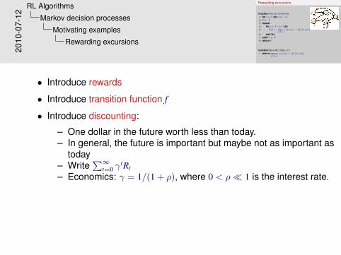
• Introduce rewards

• Introduce transition function f

• Introduce discounting:

– One dollar in the future worth less than today.– In general, the future is important but maybe not as important as

today– Write

∑∞t=0 γ

tRt

– Economics: γ = 1/(1 + ρ), where 0 < ρ� 1 is the interest rate.

Uncertainty

“Uncertainty is the only certainty there is, andknowing how to live with insecurity is the onlysecurity.” (John Allen Paulos, 1945–)

Next state might be uncertainThe reward dettoAdvantage: Richer model, robustnessA transition from X after taking action A:

Y = f (X,A,D),

R = g(X,A,D)

D – random variable; “disturbance”f – transition functiong – reward function


Uncertainty

“Uncertainty is the only certainty there is, andknowing how to live with insecurity is the onlysecurity.” (John Allen Paulos, 1945–)

Next state might be uncertainThe reward dettoAdvantage: Richer model, robustnessA transition from X after taking action A:

Y = f (X,A,D),

R = g(X,A,D)

D – random variable; “disturbance”f – transition functiong – reward function

2010

-07-

12RL Algorithms


Motivating examples

Uncertainty

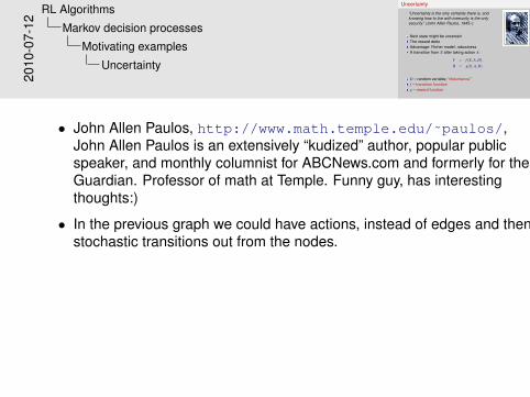
• John Allen Paulos, http://www.math.temple.edu/˜paulos/,John Allen Paulos is an extensively “kudized” author, popular publicspeaker, and monthly columnist for ABCNews.com and formerly for theGuardian. Professor of math at Temple. Funny guy, has interestingthoughts:)

• In the previous graph we could have actions, instead of edges and thenstochastic transitions out from the nodes.

http://www.math.temple.edu/~paulos/

Power management


Power management

2010

-07-

12RL Algorithms


Motivating examples

Power management

• Blurb about how important is power management

The monumental number of PCs operating worldwide createsother requirements for PC power management. Because there arehundreds of millions of PCs in operation, the installed base ofcomputers worldwide consumes tens of gigawatts for every hour ofoperation. Even small changes in average desktop computer powerconsumption can, on the global scale, save as much power asgenerated by a small power plant. (Source: Intel, http://www.intel.com/intelpress/samples/PPM_chapter.pdf)

http://www.intel.com/intelpress/samples/PPM_chapter.pdf

http://www.intel.com/intelpress/samples/PPM_chapter.pdf

Computer usage data

Sheet1

Page 1

HomeGaming 4Music entertainment 4Transcode multitasking 3Internet content creation 4Broad based productivity 36Media playback multitasking 4Windows idle 44

OfficeTranscode multitasking 2Internet content creation 3Broad based productivity 53Video content creation 1Image content creation 2Windows idle 39

http://www.amd.com/us/Documents/43029A_Brochure_PFD.pdf

Sheet1

Page 1





Source: http://www.amd.com/us/Documents/43029A_Brochure_PFD.pdf


Computer usage data

Sheet1

Page 1




Sheet1

Page 1




2010

-07-

12RL Algorithms


Motivating examples

Computer usage data

• Background: AMD surveyed over 1200 users to determine consumerand commercial usage patterns (daily time spent on each application orat idle) in four countries.

• What is important:

– Computers are often idle– They do all kind of works at other times, which require different

parts of the computer to be awake– Why is power management challenging?

F Everyone uses the computer differently.F One size fits all?? NO!

Power management

Advanced Configuration and Power Interface (ACPI)First released in December 1996, last release in June 2010Platform-independent interfaces for hardware discovery,configuration, power management and monitoring


Power management

Advanced Configuration and Power Interface (ACPI)First released in December 1996, last release in June 2010Platform-independent interfaces for hardware discovery,configuration, power management and monitoring

2010

-07-

12RL Algorithms


Motivating examples

Power management

This is a complex issue. This will be illustrated on the next two slides.The details on these slides are not so important. However, theyillustrate well the complexity of the issue.

Power mgmt – Power states

G0 (S0): WorkingG1, Sleeping subdivides into the four states S1 through S4

I S1: All processor caches are flushed, and the CPU(s) stopexecuting instructions. Power to the CPU(s) and RAM ismaintained; devices that do not indicate they must remain on maybe powered down

I S2: CPU powered offI S3: Commonly referred to as Standby, Sleep, or Suspend to RAM.

RAM remains poweredI S4: Hibernation or Suspend to Disk. All content of main memory is

saved to non-volatile memory such as a hard drive, and is powereddown

G2 (S5), Soft Off: G2 is almost the same as G3 Mechanical Off,but some components remain powered so the computer can”wake” from input from the keyboard, clock, modem, LAN, or USBdevice.G3, Mechanical Off: The computer’s power consumptionapproaches close to zero, to the point that the power cord can beremoved and the system is safe for dis-assembly (typically, onlythe real-time clock is running off its own small battery).



G0 (S0): WorkingG1, Sleeping subdivides into the four states S1 through S4

I S1: All processor caches are flushed, and the CPU(s) stopexecuting instructions. Power to the CPU(s) and RAM ismaintained; devices that do not indicate they must remain on maybe powered down

I S2: CPU powered offI S3: Commonly referred to as Standby, Sleep, or Suspend to RAM.

RAM remains poweredI S4: Hibernation or Suspend to Disk. All content of main memory is

saved to non-volatile memory such as a hard drive, and is powereddown

G2 (S5), Soft Off: G2 is almost the same as G3 Mechanical Off,but some components remain powered so the computer can”wake” from input from the keyboard, clock, modem, LAN, or USBdevice.G3, Mechanical Off: The computer’s power consumptionapproaches close to zero, to the point that the power cord can beremoved and the system is safe for dis-assembly (typically, onlythe real-time clock is running off its own small battery).

2010

-07-

12RL Algorithms


Motivating examples


Power mgmt – Device, processor, performance statesDevice states

I D0 Fully-On is the operating stateI D1 and D2 are intermediate power-states whose definition varies

by device.I D3 Off has the device powered off and unresponsive to its bus.

Processor statesI C0 is the operating state.I C1 (often known as Halt) is a state where the processor is not

executing instructions, but can return to an executing stateessentially instantaneously. All ACPI-conformant processors mustsupport this power state. Some processors, such as the Pentium 4,also support an Enhanced C1 state (C1E or Enhanced Halt State)for lower power consumption.

I C2 (often known as Stop-Clock) is a state where the processormaintains all software-visible state, but may take longer to wake up.This processor state is optional.

I C3 (often known as Sleep) is a state where the processor does notneed to keep its cache coherent, but maintains other state. Someprocessors have variations on the C3 state (Deep Sleep, DeeperSleep, etc.) that differ in how long it takes to wake the processor.This processor state is optional.

Performance states: While a device or processor operates (D0and C0, respectively), it can be in one of severalpower-performance states. These states areimplementation-dependent, but P0 is always thehighest-performance state, with P1 to Pn being successivelylower-performance states, up to an implementation-specific limit ofn no greater than 16.P-states have become known as SpeedStep in Intel processors,as PowerNow! or Cool’n’Quiet in AMD processors, and asPowerSaver in VIA processors.

I P0 max power and frequencyI P1 less than P0, voltage/frequency scaledI Pn less than P(n-1), voltage/frequency scaled


Power mgmt – Device, processor, performance statesDevice states

I D0 Fully-On is the operating stateI D1 and D2 are intermediate power-states whose definition varies

by device.I D3 Off has the device powered off and unresponsive to its bus.

Processor statesI C0 is the operating state.I C1 (often known as Halt) is a state where the processor is not

executing instructions, but can return to an executing stateessentially instantaneously. All ACPI-conformant processors mustsupport this power state. Some processors, such as the Pentium 4,also support an Enhanced C1 state (C1E or Enhanced Halt State)for lower power consumption.

I C2 (often known as Stop-Clock) is a state where the processormaintains all software-visible state, but may take longer to wake up.This processor state is optional.

I C3 (often known as Sleep) is a state where the processor does notneed to keep its cache coherent, but maintains other state. Someprocessors have variations on the C3 state (Deep Sleep, DeeperSleep, etc.) that differ in how long it takes to wake the processor.This processor state is optional.

Performance states: While a device or processor operates (D0and C0, respectively), it can be in one of severalpower-performance states. These states areimplementation-dependent, but P0 is always thehighest-performance state, with P1 to Pn being successivelylower-performance states, up to an implementation-specific limit ofn no greater than 16.P-states have become known as SpeedStep in Intel processors,as PowerNow! or Cool’n’Quiet in AMD processors, and asPowerSaver in VIA processors.

I P0 max power and frequencyI P1 less than P0, voltage/frequency scaledI Pn less than P(n-1), voltage/frequency scaled

2010

-07-

12RL Algorithms


Motivating examples

Power mgmt – Device, processor, performance states

An oversimplified model

NoteThe transitions can be represented as

Y = f (x, a,D),

R = g(x, a,D).



NoteThe transitions can be represented as

Y = f (x, a,D),

R = g(x, a,D).2010

-07-

12RL Algorithms


Motivating examples


• This is indeed oversimplified

• We could have more states

• . . . but the message should be clear.

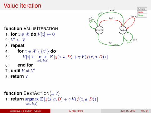
Value iteration



a∈A(x)E [g(x, a,D) + γ V( f (x, a,D)) ]


8: return V


a∈A(x)E [g(x, a,D) + γ V( f (x, a,D)) ]


Value iteration



a∈A(x)E [g(x, a,D) + γ V( f (x, a,D)) ]


8: return V


a∈A(x)E [g(x, a,D) + γ V( f (x, a,D)) ]

2010

-07-

12RL Algorithms


Motivating examples

Value iteration

• Straightforward generalization of previous algorithm:

In each step we compute the expected total reward based on theassumption that the total future rewards are given by V

• Homework: Think about the stochastic shortest path case and convinceyourself that this works.

• Question: Why does it work in general? POSTPONED!

• Show how the computation is done⇐ Excel sheet!

• IMPORTANT: Uncertainty makes it necessary to check back where youare! In deterministic problems, knowing the initial state is enough toknow how to act until you get to your goal!

How to gamble if you must?

The safest way to double your money is to fold it over onceand put it in your pocket. (“Kin” Hubbard, 1868–1930)

State Xt ≡ wealth of gambler at step t, Xt ≥ 0

Action: At ∈ [0, 1]: the fraction of Xt put at stakeSt ∈ {−1,+1}, P (St+1 = 1) = p, p ∈ [0, 1], i.i.d., random variablesFortune at next time step:

Xt+1 = (1 + St+1At)Xt.

Goal: maximize the probability that the wealth reaches w∗.How to put this into our framework?



The safest way to double your money is to fold it over onceand put it in your pocket. (“Kin” Hubbard, 1868–1930)

State Xt ≡ wealth of gambler at step t, Xt ≥ 0

Action: At ∈ [0, 1]: the fraction of Xt put at stakeSt ∈ {−1,+1}, P (St+1 = 1) = p, p ∈ [0, 1], i.i.d., random variablesFortune at next time step:

Xt+1 = (1 + St+1At)Xt.

Goal: maximize the probability that the wealth reaches w∗.How to put this into our framework?20

10-0

7-12

RL Algorithms


Motivating examples


• Frank McKinney Hubbard is an American cartoonist, humorist, andjournalist better known by his pen name ”Kin” Hubbard.

• Imagine e.g. that as a last resort you have to bet on horses because youjust need to money to pay back your debt to the mafia or you die.

How to gamble if you must? – Solution

Xt ∈ X = [0,w∗], A = [0, 1]

Let f : X ×A× {−1,+1} → X be

f (x, a, s) =

{(1 + s a)x ∧ w∗, if x < w∗;w∗, otherwise.

Let g : X ×A× {−1,+1} → X be

g(x, a, s) =

{1, if (1 + s a)x ≥ w∗ and x < w∗;0, otherwise.

What is the optimal policy?



Xt ∈ X = [0,w∗], A = [0, 1]

Let f : X ×A× {−1,+1} → X be

f (x, a, s) =

{(1 + s a)x ∧ w∗, if x < w∗;w∗, otherwise.

Let g : X ×A× {−1,+1} → X be

g(x, a, s) =

{1, if (1 + s a)x ≥ w∗ and x < w∗;0, otherwise.

What is the optimal policy?2010

-07-

12RL Algorithms


Motivating examples


• Mention that this is an episodic problem

• The strange tent-like symbol, ∧, is a binary operator, similar to, say, +. Itcomputes the minimum of its arguments.

• Here w∗ is an absorbing state

• This is a prototypical example of how we can deal with problems whenthe goal is to maximize the probability of an event

• Ask audience: How would you play this game?

• How to compute the optimal value function?

The state space became infinite..

• Optimal strategy: “bold strategy” (no need to tell them)– Risk the smallest of the amount missing to reach w∗ and your

current wealth

Inventory control

19:00

7:00

14:00

X = {0, 1, . . . ,M}; Xt size of the inventory in the evening of day t

A = {0, 1, . . . ,M}; At number of items ordered in the evening of day t

Dynamics:Xt+1 = ((Xt + At) ∧M − Dt+1)

+.

Reward:

Rt+1 = −K I{At>0} − c ((Xt + At) ∧M − Xt)+

− h Xt + p ((Xt + At) ∧M − Xt+1)+.


Inventory control

19:00

7:00

14:00

X = {0, 1, . . . ,M}; Xt size of the inventory in the evening of day t

A = {0, 1, . . . ,M}; At number of items ordered in the evening of day t

Dynamics:Xt+1 = ((Xt + At) ∧M − Dt+1)

+.

Reward:

Rt+1 = −K I{At>0} − c ((Xt + At) ∧M − Xt)+

− h Xt + p ((Xt + At) ∧M − Xt+1)+.

2010

-07-

12RL Algorithms


Motivating examples

Inventory control

• Explanation of the quantities involved:

– M – maximum inventory size– Dt+1 – demand– K – fixed cost of ordering any items– c – cost of lost sales– h – inventory cost– p – sales proceeds

• Zt = (Xt + At) ∧M – post-decision state, or afterstate

This also comes up in games

Other examples

Engineering, operations researchI Process control

F ChemicalF ElectronicF Mechanical systems⇒ ROBOTS

I Supply chain managementInformation theory

I optimal codingI channel allocationI sensing, sensor networks

FinanceI portfolio managementI option pricing

Artificial intelligenceI The whole problem of acting under uncertaintyI SearchI GamesI Vision: Gaze controlI Information retrieval

...Szepesvari & Sutton (UofA) RL Algorithms July 11, 2010 23 / 51

Other examples

Engineering, operations researchI Process control

F ChemicalF ElectronicF Mechanical systems⇒ ROBOTS

I Supply chain managementInformation theory

I optimal codingI channel allocationI sensing, sensor networks

FinanceI portfolio managementI option pricing

Artificial intelligenceI The whole problem of acting under uncertaintyI SearchI GamesI Vision: Gaze controlI Information retrieval

...

2010

-07-

12RL Algorithms


Motivating examples

Other examples

• The point is, these problems are ubiquous.

• TODO: Add some figures

Controlled Markov processes

Xt+1 = f (Xt,At,Dt+1) State dynamicsRt+1 = g(Xt,At,Dt+1) Reward

t = 0, 1, . . . .

Xt ∈ X – state at time t

X – set of statesAt ∈ A – action at time t

A – set of actionsSometimes, A(x): admissible actionsRt+1 ∈ R – reward⇒ RDt ∈ D – disturbance; i.i.d. sequenceD – disturbance space



Xt+1 = f (Xt,At,Dt+1) State dynamicsRt+1 = g(Xt,At,Dt+1) Reward

t = 0, 1, . . . .

Xt ∈ X – state at time t

X – set of statesAt ∈ A – action at time t

A – set of actionsSometimes, A(x): admissible actionsRt+1 ∈ R – reward⇒ RDt ∈ D – disturbance; i.i.d. sequenceD – disturbance space

2010

-07-

12RL Algorithms




This just collects on a single slide what we have talked about before.

Return

Definition (Return)Return, or total discounted return is:

R =

∞∑t=0

γtRt+1,

where 0 ≤ γ ≤ 1 is the so-called discount factor. The return dependson how we act!


Return

Definition (Return)Return, or total discounted return is:

R =

∞∑t=0

γtRt+1,

where 0 ≤ γ ≤ 1 is the so-called discount factor. The return dependson how we act!

2010

-07-

12RL Algorithms



Return

• The return is an important quantity.

• Return 6= immediate reward (or, just reward)

• The index goes fro time step zero, but the “zero” can be shifted around

• If the rewards are bounded in expectation and the discount factor γ isless than one then the expected return is well defined.

• If the rewards can be unbounded (from below, or above), care must betaken, e.g., Gaussian noise..

• The discount factor could be one, but then one must be careful becausethe return might become unbounded, even when the rewards arebounded

The goal of control

GoalMaximize the expected total discounted reward, or expected return,irrespective of the initial state:

E

[ ∞∑t=0

γtRt+1 |X0 = x

]→ max!, x ∈ X .


The goal of control

GoalMaximize the expected total discounted reward, or expected return,irrespective of the initial state:

E

[ ∞∑t=0

γtRt+1 |X0 = x

]→ max!, x ∈ X .

2010

-07-

12RL Algorithms



The goal of control

• Note that there is no distribution over the states.

• We want to act optimally from each state

• For each state, a different “policy” might be optimal.

Alternate definition

Definition (Markov decision process)Triplet: (X ,A,P0), whereX – set of statesA – set of actionsP0 – state and reward kernelP0(U|x, a) is the probability that (Xt+1,Rt+1) lands in U ⊂ X × Rgiven that Xt = x, At = a


Alternate definition

Definition (Markov decision process)Triplet: (X ,A,P0), whereX – set of statesA – set of actionsP0 – state and reward kernelP0(U|x, a) is the probability that (Xt+1,Rt+1) lands in U ⊂ X × Rgiven that Xt = x, At = a

2010

-07-

12RL Algorithms


Alternate definitionsAlternate definition

• Somewhat unconventional definition, but very compact at least,and very general, too

Connection to previous definition

Assume that

Xt+1 = f (Xt,At,Dt+1)

Rt+1 = g(Xt,At,Dt+1)

t = 0, 1, . . . .

ThenP0(U| x, a) = P ( [ f (x, a,D), g(x, a,D)] ∈ U ) ,

Here, D has the same distribution as D1,D2, . . ..


Connection to previous definition

Assume that

Xt+1 = f (Xt,At,Dt+1)

Rt+1 = g(Xt,At,Dt+1)

t = 0, 1, . . . .

ThenP0(U| x, a) = P ( [ f (x, a,D), g(x, a,D)] ∈ U ) ,

Here, D has the same distribution as D1,D2, . . ..2010

-07-

12RL Algorithms


Alternate definitionsConnection to previous definition

• The two definitions, in fact, are equivalent.

• Sometimes this, sometimes the other definition is the more convenient

“Classical form”

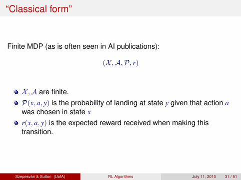
Finite MDP (as is often seen in AI publications):

(X ,A,P, r)

X ,A are finite.P(x, a, y) is the probability of landing at state y given that action awas chosen in state x

r(x, a, y) is the expected reward received when making thistransition.


“Classical form”

Finite MDP (as is often seen in AI publications):

(X ,A,P, r)

X ,A are finite.P(x, a, y) is the probability of landing at state y given that action awas chosen in state x

r(x, a, y) is the expected reward received when making thistransition.

2010

-07-

12RL Algorithms


Alternate definitions“Classical form”

• This is a smaller class

• But if X , A are allowed to be countably infinite, the analysis can getpretty complicated.

• What is lost is our ability to talk about continuity:

– The naming of states, actions is arbitrary!!– In continuous problems, we often have some sort of continuity,

allowing for generalization to “nearby” states/actions!– This could be mimicked by introducing some kind of “distance

function”

Policies, values

NoteFrom now on we assume that A is countable.

Definition (General policy)Maps each history to a distribution over A.Deterministic policy: π = (π0, π1, . . .), where π0 : X → A andπt : (X ×A× R)t−1 ×X → A, t = 1, 2, . . ..Following the policy: At = πt(X0,A0,R1, . . . ,Xt−1,At−1,Rt,Xt).


Policies, values

NoteFrom now on we assume that A is countable.

Definition (General policy)Maps each history to a distribution over A.Deterministic policy: π = (π0, π1, . . .), where π0 : X → A andπt : (X ×A× R)t−1 ×X → A, t = 1, 2, . . ..Following the policy: At = πt(X0,A0,R1, . . . ,Xt−1,At−1,Rt,Xt).

2010

-07-

12RL Algorithms


Policies, valuesPolicies, values

• General policies: When we do learning, we follow a general policy,because the policy depends on the history!

• Usually the history is compressed in some form

Stationary policies

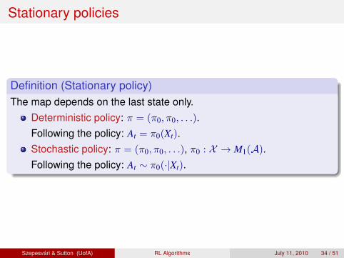
Definition (Stationary policy)The map depends on the last state only.

Deterministic policy: π = (π0, π0, . . .).Following the policy: At = π0(Xt).Stochastic policy: π = (π0, π0, . . .), π0 : X → M1(A).Following the policy: At ∼ π0(·|Xt).


Stationary policies

Definition (Stationary policy)The map depends on the last state only.

Deterministic policy: π = (π0, π0, . . .).Following the policy: At = π0(Xt).Stochastic policy: π = (π0, π0, . . .), π0 : X → M1(A).Following the policy: At ∼ π0(·|Xt).

2010

-07-

12RL Algorithms


Policies, valuesStationary policies

• We just identify π and π0.

• Stationary policies has a distinctive role in the theory of MDPs

The value of a policy

Definition (Value of a state under π)The expected return given that the policy is started in state x:

Vπ(x) = E [Rπ|X0 = x] .

Vπ – value function of π.

Definition (Action-value of a state-action pair under π)The expected return given that the process is started from state x, thefirst action is a after which the policy π is followed:

Qπ(x, a) = E [Rπ|X0 = x,A0 = a] .

Qπ – action-value function of π


The value of a policy

Definition (Value of a state under π)The expected return given that the policy is started in state x:

Vπ(x) = E [Rπ|X0 = x] .

Vπ – value function of π.

Definition (Action-value of a state-action pair under π)The expected return given that the process is started from state x, thefirst action is a after which the policy π is followed:

Qπ(x, a) = E [Rπ|X0 = x,A0 = a] .

Qπ – action-value function of π2010

-07-

12RL Algorithms


Policies, valuesThe value of a policy

• These are well-defined under our conditions.

• Even for general policies.

• The action-values were introduced by Watkins; they are very useful aswe shall see later.

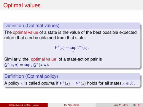
Optimal values

Definition (Optimal values)The optimal value of a state is the value of the best possible expectedreturn that can be obtained from that state:

V∗(x) = supπ

Vπ(x).

Similarly, the optimal value of a state-action pair isQ∗(x, a) = supπ Qπ(x, a).

Definition (Optimal policy)A policy π is called optimal if Vπ(x) = V∗(x) holds for all states x ∈ X .


Optimal values

Definition (Optimal values)The optimal value of a state is the value of the best possible expectedreturn that can be obtained from that state:

V∗(x) = supπ

Vπ(x).

Similarly, the optimal value of a state-action pair isQ∗(x, a) = supπ Qπ(x, a).

Definition (Optimal policy)A policy π is called optimal if Vπ(x) = V∗(x) holds for all states x ∈ X .20

10-0

7-12

RL Algorithms


Policies, valuesOptimal values

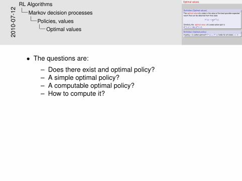
• The questions are:

– Does there exist and optimal policy?– A simple optimal policy?– A computable optimal policy?– How to compute it?

The fundamental theorem and the Bellman (optimality) operator

TheoremAssume that |A| < +∞. Then the optimal value function satisfies

V∗(x) = maxa∈A

r(x, a) + γ∑y∈XP(x, a, y)V∗(y)

, x ∈ X .

and if policy π is such that in each state x it selects an action that maximizesthe r.h.s. then π is an optimal policy.

A shorter way to write this isV∗ = T∗V∗,

(T∗V)(x) = maxa∈A

r(x, a) + γ∑y∈XP(x, a, y)V(y)

, x ∈ X .


The fundamental theorem and the Bellman (optimality) operator

TheoremAssume that |A| < +∞. Then the optimal value function satisfies

V∗(x) = maxa∈A

r(x, a) + γ∑y∈XP(x, a, y)V∗(y)

, x ∈ X .

and if policy π is such that in each state x it selects an action that maximizesthe r.h.s. then π is an optimal policy.

A shorter way to write this isV∗ = T∗V∗,

(T∗V)(x) = maxa∈A


, x ∈ X .2010

-07-

12RL Algorithms

Theory of dynamic programming

The fundamental theoremThe fundamental theorem and the Bellman(optimality) operator

• Explain that operators are just functions that act on functions, butfunctions are really like vectors, so no one should be afraid of this.

• What is the history? Hard to tell. The theorem exists in variousgeneralities. This simple form must have been known to Bellman(1920–1984), who “invented” dynamic programming in 1953. Dreyfus,Blackwell and others worked out the math for the more complicatedcases and there is still work left. Some older economics literaturementioned the principle of optimality.

Action evaluation operator

Definition (Action evaluation operator)Let a ∈ A and define

(TaV)(x) = r(x, a) + γ∑y∈XP(x, a, y)V(y), x ∈ X .

Comment

T∗V [x] = maxa∈A

TaV [x].


Action evaluation operator

Definition (Action evaluation operator)Let a ∈ A and define

(TaV)(x) = r(x, a) + γ∑y∈XP(x, a, y)V(y), x ∈ X .

Comment

T∗V [x] = maxa∈A

TaV [x].2010

-07-

12RL Algorithms


The fundamental theoremAction evaluation operator

Policy evaluation operator

Definition (Policy evaluation operator)Let π be a stochastic stationary policy. Define

(TπV)(x) =∑a∈A

π(a|x)


=

∑a∈A

π(a|x)TaV(x), x ∈ X .

CorollaryTπ is a contraction, and Vπ is the unique fixed point of Tπ.


Policy evaluation operator

Definition (Policy evaluation operator)Let π be a stochastic stationary policy. Define

(TπV)(x) =∑a∈A

π(a|x)


=

∑a∈A

π(a|x)TaV(x), x ∈ X .

CorollaryTπ is a contraction, and Vπ is the unique fixed point of Tπ.

2010

-07-

12RL Algorithms


The fundamental theoremPolicy evaluation operator

Greedy policy

Definition (Greedy policy)Policy π is greedy w.r.t. V if

TπV = T∗V,

or

∑a∈A

π(a|x)


=

maxa∈A

{r(x, a) + γ

∑y∈X P(x, a, y)V(y)

}holds for all states x.


Greedy policy

Definition (Greedy policy)Policy π is greedy w.r.t. V if

TπV = T∗V,

or

∑a∈A

π(a|x)


=

maxa∈A

{r(x, a) + γ

∑y∈X P(x, a, y)V(y)

}holds for all states x.20

10-0

7-12

RL Algorithms


The fundamental theoremGreedy policy

A restatement of the main theorem

TheoremAssume that |A| < +∞. Then the optimal value function satisfies thefixed-point equation V∗ = T∗V∗ and any greedy policy w.r.t. V∗ isoptimal.


A restatement of the main theorem

TheoremAssume that |A| < +∞. Then the optimal value function satisfies thefixed-point equation V∗ = T∗V∗ and any greedy policy w.r.t. V∗ isoptimal.

2010

-07-

12RL Algorithms


The fundamental theoremA restatement of the main theorem

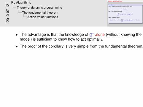
Action-value functions

CorollaryLet Q∗ be the optimal action-value function. Then,

Q∗ = T∗Q∗

and if π is a policy such that∑a∈A

π(a|x)Q∗(x, a) = maxa∈A

Q∗(x, a)

then π is optimal. Here,

T∗Q (x, a) = r(x, a) + γ∑y∈XP(x, a, y)max

a′∈AQ(y, a′), x ∈ X , a ∈ A.


Action-value functions

CorollaryLet Q∗ be the optimal action-value function. Then,

Q∗ = T∗Q∗

and if π is a policy such that∑a∈A

π(a|x)Q∗(x, a) = maxa∈A

Q∗(x, a)

then π is optimal. Here,

T∗Q (x, a) = r(x, a) + γ∑y∈XP(x, a, y)max

a′∈AQ(y, a′), x ∈ X , a ∈ A.20

10-0

7-12

RL Algorithms


The fundamental theoremAction-value functions

• The advantage is that the knowledge of Q∗ alone (without knowing themodel) is sufficient to know how to act optimally.

• The proof of the corollary is very simple from the fundamental theorem.

Finding the action-value functions of policies

TheoremLet π be a stationary policy, Tπ be defined by

TπQ (x, a) = r(x, a) + γ∑y∈XP(x, a, y)

∑a′∈A

π(a′|y)Q(y, a′), x ∈ X , a ∈ A.

Then Qπ is the unique solution of

TπQπ = Qπ.


Finding the action-value functions of policies

TheoremLet π be a stationary policy, Tπ be defined by

TπQ (x, a) = r(x, a) + γ∑y∈XP(x, a, y)

∑a′∈A

π(a′|y)Q(y, a′), x ∈ X , a ∈ A.

Then Qπ is the unique solution of

TπQπ = Qπ.

2010

-07-

12RL Algorithms


The fundamental theoremFinding the action-value functions of policies

Value iteration – a second look


1: for x ∈ X do V[x]← 02: V ′ ← V3: repeat4: for x ∈ X \ {x∗} do5: V[x]← T∗V [x]6: end for7: until V 6= V ′

8: return V


a∈A(x)TaV [x]




1: for x ∈ X do V[x]← 02: V ′ ← V3: repeat4: for x ∈ X \ {x∗} do5: V[x]← T∗V [x]6: end for7: until V 6= V ′

8: return V


a∈A(x)TaV [x]20

10-0

7-12

RL Algorithms


Algorithms of dynamic programming


• Asynchronous updates have been studied.

• Also, “labelled value iteration” tries to keep track of what needs to beupdated.

• Another variation is real-time dynamic programming (RTDP), which isrelated to Korf’s LRTA∗.

• With optimistic initialization this is known to converge.

• Optimistic initialization ≡ admissible heuristics!

Value iteration

NoteIf Vt is the value-function computed in the tth iteration of valueiteration then

Vt+1 = T∗Vt.

The key is that T∗ is a contraction in the supremum norm andBanach’s fixed-point theorem gives the key to the proof thetheorem mentioned before.

NoteOne can also use Qt+1 = T∗Qt, or value functions with post-decisionstates. What is the advantage?


Value iteration

NoteIf Vt is the value-function computed in the tth iteration of valueiteration then

Vt+1 = T∗Vt.

The key is that T∗ is a contraction in the supremum norm andBanach’s fixed-point theorem gives the key to the proof thetheorem mentioned before.

NoteOne can also use Qt+1 = T∗Qt, or value functions with post-decisionstates. What is the advantage?

2010

-07-

12RL Algorithms



Value iteration

Policy iteration

function POLICYITERATION(π)1: repeat2: π′ ← π3: V ← GETVALUEFUNCTION(π′)4: π ← GETGREEDYPOLICY(V)5: until π 6= π′

6: return π


Policy iteration

function POLICYITERATION(π)1: repeat2: π′ ← π3: V ← GETVALUEFUNCTION(π′)4: π ← GETGREEDYPOLICY(V)5: until π 6= π′

6: return π

2010

-07-

12RL Algorithms



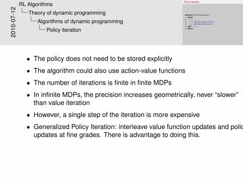
Policy iteration

• The policy does not need to be stored explicitly

• The algorithm could also use action-value functions

• The number of iterations is finite in finite MDPs

• In infinite MDPs, the precision increases geometrically, never “slower”than value iteration

• However, a single step of the iteration is more expensive

• Generalized Policy Iteration: interleave value function updates and policyupdates at fine grades. There is advantage to doing this.

What if we stop early?

Theorem (e.g., Corollary 2 of Singh and Yee 1994)Fix an action-value function Q and let π be a greedy policy w.r.t. Q.Then the value of policy π can be lower bounded as follows:

Vπ(x) ≥ V∗(x)− 21− γ

‖Q− Q∗‖∞, x ∈ X .



Theorem (e.g., Corollary 2 of Singh and Yee 1994)Fix an action-value function Q and let π be a greedy policy w.r.t. Q.Then the value of policy π can be lower bounded as follows:

Vπ(x) ≥ V∗(x)− 21− γ

‖Q− Q∗‖∞, x ∈ X .

2010

-07-

12RL Algorithms




Books

Bertsekas and Shreve (1978)Puterman (1994)Bertsekas (2007a,b)


Books

Bertsekas and Shreve (1978)Puterman (1994)Bertsekas (2007a,b)

2010

-07-

12RL Algorithms



Books

References

Bertsekas, D. P. (2007a). Dynamic Programming and Optimal Control,volume 1. Athena Scientific, Belmont, MA, 3 edition.

Bertsekas, D. P. (2007b). Dynamic Programming and Optimal Control,volume 2. Athena Scientific, Belmont, MA, 3 edition.

Bertsekas, D. P. and Shreve, S. (1978). Stochastic Optimal Control(The Discrete Time Case). Academic Press, New York.

Puterman, M. (1994). Markov Decision Processes — DiscreteStochastic Dynamic Programming. John Wiley & Sons, Inc., NewYork, NY.

Singh, S. P. and Yee, R. C. (1994). An upper bound on the loss fromapproximate optimal-value functions. Machine Learning,16(3):227–233.


References

Bertsekas, D. P. (2007a). Dynamic Programming and Optimal Control,volume 1. Athena Scientific, Belmont, MA, 3 edition.

Bertsekas, D. P. (2007b). Dynamic Programming and Optimal Control,volume 2. Athena Scientific, Belmont, MA, 3 edition.

Bertsekas, D. P. and Shreve, S. (1978). Stochastic Optimal Control(The Discrete Time Case). Academic Press, New York.

Puterman, M. (1994). Markov Decision Processes — DiscreteStochastic Dynamic Programming. John Wiley & Sons, Inc., NewYork, NY.

Singh, S. P. and Yee, R. C. (1994). An upper bound on the loss fromapproximate optimal-value functions. Machine Learning,16(3):227–233.20

10-0

7-12

RL Algorithms

Bibliography

References