Centre for Risk & Insurance Studies

enhancing the understanding of risk and insurance

OPTIONS ON NORMAL UNDERLYINGS

Paul Dawson, David Blake, Andrew J G Cairns, Kevin Dowd

CRIS Discussion Paper Series – 2007.VII

OPTIONS ON NORMAL UNDERLYINGS

Abstract The seminal option pricing work of Black and Scholes [1973] and Merton [1973] was predicated on the price of the underlying asset being lognormally distributed. Ever since it became clear that a geometric Brownian motion process provides a more plausible model of asset prices than its arithmetic equivalent, it has been assumed that an option pricing model for a normally distributed underlying asset was redundant. Nevertheless, 34 years after Black and Scholes [1973] and Merton [1973], we identify a contemporary need for such a model: namely when we wish to price an option on a survivor swap. In this case, an option-pricing model based on a normal underlying is not some flawed relative of Black-Scholes, as it is usually considered to be, but is instead the key to pricing this type of swaption correctly – and hence, a very useful tool in the rapidly emerging universe of mortality derivatives. Accordingly, this paper derives the call and put valuation models for options on normal underlying assets, and derives their Greeks. It then shows how this option pricing model can be used to price swaptions on survivor swaps.

Paul Dawson David Blake

Andrew J G Cairns Kevin Dowd

This version:19 November 2007

PRELIMINARY VERSION – COMMENTS WELCOME. NOT TO BE QUOTED WITHOUT PERMISSION FROM AUTHORS

Corresponding author: Paul Dawson, Kent State University, e-mail:pdawson1@kent.edu

1

OPTIONS ON NORMAL UNDERLYINGS

1. Introduction

The seminal option pricing work of Black and Scholes [1973] and Merton [1973] was

predicated on the assumption that the geometric (or continuously compounded) returns of the

asset under option are normally distributed, or equivalently, that prices of that asset are

lognormally distributed. Subsequent research (e.g. Cox and Ross [1976]) has considered other

distributions and, especially since Rubinstein [1994], research has analyzed the distributions

implied in market prices of options across a range of strike prices.

One case which has not been given much attention is that in which the price of an

asset, rather than its returns, is normally distributed. This case was famously considered by

Bachelier’s model of arithmetic Brownian motion (Bachelier [1900]). However, such a

distribution would allow the underlying asset price to become negative, and this uncomfortable

implication can be avoided by using a geometric Brownian motion (GBM) instead.

Consequently, the Bachelier model came to be was regarded as an instructive dead end. The

lack of interest in an option-pricing model with a normally distributed underlying was

therefore hardly surprising.

Nonetheless, we suggest here that it is premature to conclude that an option pricing

model with a normal underlying is of no use. An example of such a requirement arises from

some recent work on survivor derivatives. Dowd, Blake, Cairns and Dawson [2006] identify a

premium, π, in the pricing of survivor swaps, which must be permitted to become negative.

Dawson, Blake, Cairns and Dowd [2007] then go on to establish that π is the essential

stochastic variable in the pricing of survivor swaptions, and further show that the distribution

2

of π is approximately normal. Thus, pricing a survivor swaption requires an option pricing

model with a normal underlying.

The principal purpose of the present paper is to provide such a model. Accordingly,

section 2 derives the formulae for the call and put options for a European option with a

normal underlying and presents their Greeks. Section 3 discusses how the model can be

applied to price swaptions on survivor swaps. Section 4 tests the model and section 5

concludes. The derivation of the Greeks is presented in the appendix.

2. Model Derivation

For the remainder of the paper, we consider an asset with forward price F, with -∞ < F < ∞. We

do not consider the case of an option on a normally distributed spot price, as this is an obvious

special case of an option on a forward price. We denote the value of European call and put

options by c and p respectively. The strike price and maturity of the options are denoted by X

and τ respectively. The annual risk-free interest rate is denoted by r and the annual volatility

rate (or the annual standard deviation of the price of the asset) is denoted by σ.

We first establish the put-call parity condition. The put-call parity condition for the

options under consideration in the present paper is the same as that applicable in Black [1976]

for options on forward contracts with lognormally distributed prices, i.e.

( ) ( )τ−= − F-X rp c e 1

Proof of this condition follows the same reasoning as Stoll [1969]. Consider an investor who

holds a call option in tandem with a short position in an otherwise identical put. At maturity,

either the investor will choose to exercise the call option or the put option will be exercised

against him/her. Either way, the investor will acquire the forward contract at the strike price,

3

X. The investor has thus replicated a forward contract at a price of X. A zero value forward

contract has a price of F. The forward value of the portfolio of long call and short put is thus F

– X. Its present value is then e-rτ(F – X) and it follows that

( ) ( )( ) ( )

τ

τ

−

−

− = −

∴ = − −

r

r

c p e F X

p c e F X

2

3 QED

The Black-Scholes-Merton dynamic hedging strategy can be implemented if there is

assumed to be a liquid market in the underlying asset. In such circumstances, a risk-free

portfolio of asset and option can be constructed and the value of an option is simply the

present value of its expected payoff. The values of call and put options can then be presented as

( ) ( )( ) ( )( ) ( )( ) ( )

ττ τ τ

ττ τ τ

−

−

= × > × > −

= × < × − <

|

|

r

r

c e P F X E F F X X

p e P F X X E F F X

4

5

in which Fτ represents the forward price at option expiry, and Fτ ~N(F,σ2τ).

If N(z) is the standard normal cumulative density function of z, with z ~ N(0,1), the

corresponding probability density function, , is: )(' zN

( )π

−=

2

21

'( ) 2

z

N z e 6

and it follows that

( )( )

( )

( )

( )

σ ττ

σ τ

π

π

−−∞

−−

−∞

> =

= −

∫

∫

2

2

2

2

2

2

1

2

11

2

X F

X

X FX

P F X e dF

e dF

7

8

Defining σ

−=

F X

td then gives:

4

( ) ( )

( )

( ) ( )

σ τ

σ τ

− > = −

− =

=

1

X FP F X N

F XN

N d

9

10

11

We next consider the conditional expected value of Fτ, i.e. the expected value of F at

expiry given that the call option has expired in the money:

( )

( )

( )( )

τ σ τ

τ τ

σ τ

π

π

−−∞

−−∞

> =∫

∫

2

2

2

2

2

2

2| 12

X F

X

X F

X

Fe dF

E F F X

e dF

12

A well-known result from expected shortfall theory – see, e.g. Dowd [2005, pp. 154] -

shows that:

( )

( )( )

( )( )

( )

( )( )

( )

τ σ τ

σ τ

σ τπ σ τ

σ τπ

σ τ

σ τ

−−∞

−−∞

− = +

− −

−= +

− −

= +

∫

∫

2

2

2

2

2

2

' 2 1 12

'

1

'

X F

X

X F

X

X FF Ne dFF

X FNe dF

N dF

N d

N dF

N d

13

14

15

Substituting (11) and (15) into (4) gives:

( ) ( )( )

( )τ σ τ− = × × + −

' r N d

c e N d F XN d

16

and so gives us the call option pricing formula we are seeking in (17) below.

( ) ( ) ( )( ) ( )τ σ τ−= − + ' rc e F X N d N d 17

Substituting (17) into (3) then gives

5

( ) ( ) ( )( ) ( )

( ) ( )( ) ( )( ) ( )

( ) ( )( ) ( )( ) ( )

τ τ

τ

τ

σ τ

σ τ

σ τ

− −

−

−

= − + − +

= − − +

= − − +

'

1 '

1 '

r r

r

r

p e F X N d N d F Xe

e F X N d N d

e X F N d N d

18

19

20

Thus, the corresponding put option formula is given by (21) below.

( ) ( ) ( )( ) ( )τ σ τ−= − − + ' rp e X F N d N d 21

Table 1 presents the Greeks. Their derivation can be found in the appendix.

Insert Table 1 about here

3. A practical application

As noted earlier, a practical illustration of the usefulness of this option pricing model can be

found in the pricing of survivor swaptions or options on survivor swaps. Dowd et al. [2006]

propose a survivor swap contract in which the receive-fixed party commits to making a payment

stream based on the actual survivorship rate of a specified cohort and receives in return a fixed

payment stream, based on the expected survivorship rate of that cohort expected at the time of

the swap contract formation multiplied by (1+π). The term π is a risk premium reflecting the

potential errors in the expectation and π can be positive or negative, depending on whether

greater longevity (π > 0) or lesser longevity (π < 0) is perceived to be the greater risk. It can also

be zero, when the risks of greater longevity and lesser longevity exactly balance. Typically,

however, we would expect π to be in the region close to zero, and in this region, and Dawson et

al. [2007] go on to show that the distribution of π is approximately normal when underlying

aggregate mortality shocks obey the beta process set out in Dowd et al. [2006, pp. 5-7]. They

then propose a European survivor swaption contract, in which the option holder has the right,

but not the obligation, to enter into a survivor swap contract on pre-specified terms at some

time in the future. These options can take one of two forms: a payer swaption, equivalent to

6

our earlier call, in which the holder has the right but not the obligation to enter into a pay-

fixed swap at the specified future time; and a receiver swaption, equivalent to our earlier put, in

which the holder has the right but not the obligation to enter into a receive-fixed swap at the

specified future time.

In order to price the swaption using the usual dynamic hedging strategies assumed for

pricing purposes, we are also implicitly assuming that there is a liquid market in the underlying

asset, the forward survivor swap. Naturally, we recognize that this assumption is not yet

empirically valid, but we would defend it as a natural starting point, not least since survivor

swaptions cannot exist without survivor swaps.

We now consider an example calibrated on swaptions that mature in 5 years’ time and

are based on a cohort of US males who will be 70 when the swaptions mature. The strike price

of the swaption is a specified value of π and for this example, we shall use an at-the-money

forward option, i.e. X is set at the prevailing level of π for the forward contract used to hedge

the swaption. Setting the option at the money forward means that the payer swaption premium

and the receiver swaption premium are identical at all times.

Using the same mortality table as Dowd et al. [2006], and assuming, as they did,

longevity shocks, εi, drawn from a beta distribution1 with parameters 1000 and 1000 and a

yield curve flat at 6%, Monte Carlo analysis with 10,000 trials shows the distribution of π for

the forward swap to have the following values:

Mean 0.001156

Annual variance 0.000119 Skewness 0.008458 Kurtosis 3.029241

1 See Dowd et al [2006] for the significance of the longevity shocks, εi, and the beta distribution..

7

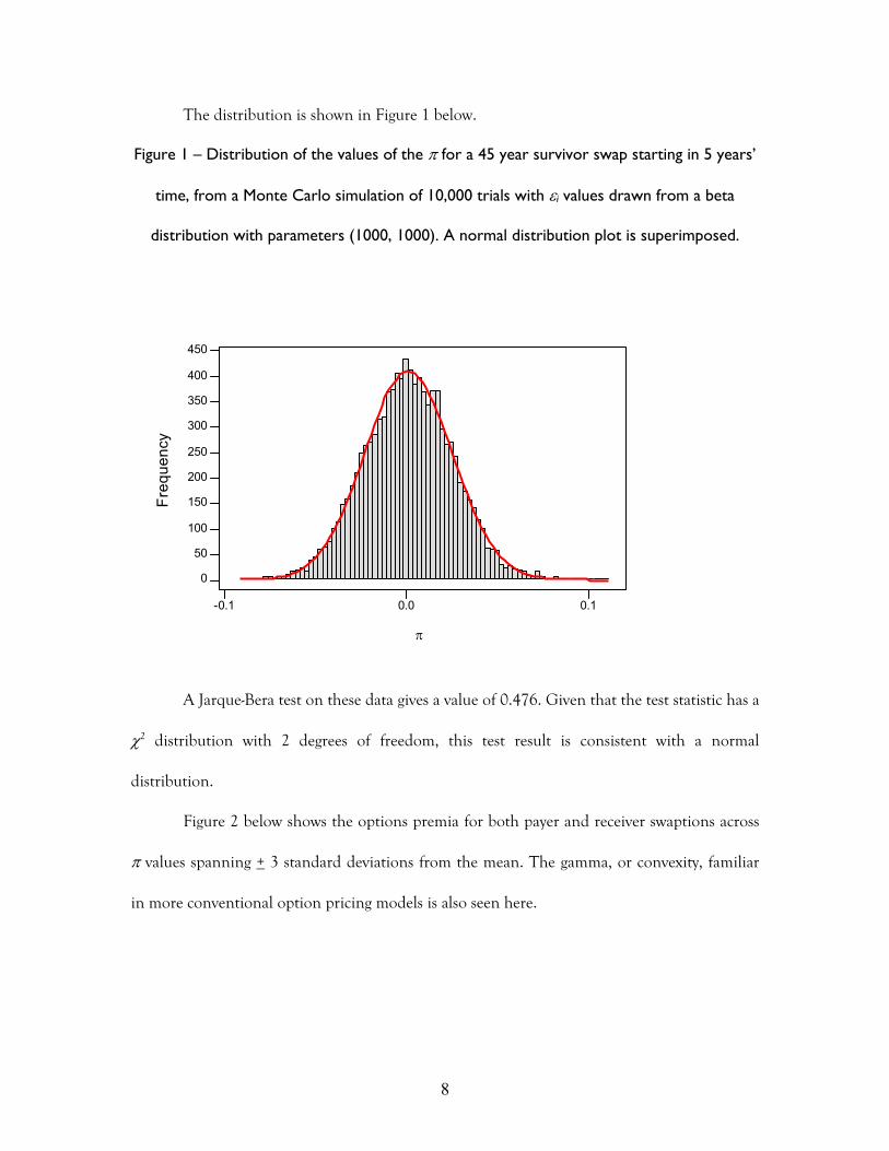
The distribution is shown in Figure 1 below.

Figure 1 – Distribution of the values of the π for a 45 year survivor swap starting in 5 years’

time, from a Monte Carlo simulation of 10,000 trials with εi values drawn from a beta

distribution with parameters (1000, 1000). A normal distribution plot is superimposed.

-0.1 0.0 0.1

0

50

100

150

200

250

300

350

400

450

Frequency

π

A Jarque-Bera test on these data gives a value of 0.476. Given that the test statistic has a

χ2 distribution with 2 degrees of freedom, this test result is consistent with a normal

distribution.

Figure 2 below shows the options premia for both payer and receiver swaptions across

π values spanning + 3 standard deviations from the mean. The gamma, or convexity, familiar

in more conventional option pricing models is also seen here.

8

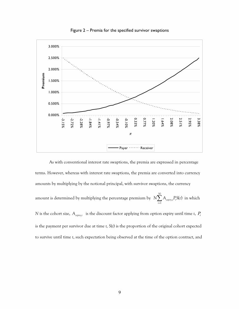
Figure 2 – Premia for the specified survivor swaptions

0.000%

0.500%

1.000%

1.500%

2.000%

2.500%

3.000%

-3.15%

-2.72%

-2.28%

-1.84%

-1.41%

-0.97%

-0.54%

-0.10%

0.33%

0.77%

1.20%

1.64%

2.08%

2.51%

2.95%

3.38%

π

Pre

miu

m

Payer Receiver

As with conventional interest rate swaptions, the premia are expressed in percentage

terms. However, whereas with interest rate swaptions, the premia are converted into currency

amounts by multiplying by the notional principal, with survivor swaptions, the currency

amount is determined by multiplying the percentage premium by in which

N is the cohort size, is the discount factor applying from option expiry until time t,

is the payment per survivor due at time t, S(t) is the proportion of the original cohort expected

to survive until time t, such expectation being observed at the time of the option contract, and

=∑50

,1

( )expiry t tt

N A P S t

,expiry tA tP

9

where all members of the cohort are assumed to be dead after 50 years.2 N A is

known with certainty at the time of option pricing.

=∑50

1

( )expiry,t tt

P S t

1 0.5

Figure 3 below shows the changing value of these at the money forward payer and

receiver swaptions as time passes. The rapid price decay as expiry approaches, again familiar in

more conventional options, is also seen here.

Figure 3 – Options premia against time

0.0000%

0.1000%

0.2000%

0.3000%

0.4000%

0.5000%

0.6000%

0.7000%

0.8000%

5 4.5 4 3.5 3 2.5 2 1.5 0

Years to expiry

Pre

miu

m

2 This approach is equivalent to that used in the pricing of an amortizing interest rate swap, in which the notional principal is reduced by pre-specified amounts over the life of the swap contract.

10

4. Testing the model

The derivation of the model is predicated on the assumption that implementation of a

dynamic hedging strategy will eliminate the risk of holding long or short positions in such

options. We test the effectiveness of this strategy by simulating the returns to dealers with

(separate) short3 positions in payer and receiver swaptions, and who undertake daily rehedging

over the 5 year (1,250 trading days) life of the swaptions. We use Monte Carlo simulation to

model the evolution of the underlying forward swap price, assuming a normal distribution. We

assume a dealer starting off with zero cash and borrowing or depositing at the risk-free rate in

response to the cashflows generated by the dynamic hedging strategy. As Merton [1973, p165]

states, “Since the portfolio requires zero investment, it must be that to avoid “arbitrage” profits,

the expected (and realized) return on the portfolio with this strategy is zero.” Merton’s model

was predicated on rehedging in continuous time, which would lead to expected and realized

returns being identical. In practice, traders are forced to use discrete time rehedging, which is

modeled here. One consequence of this is that on any individual simulation, the realized

return may differ from zero, but that over a large number of simulations, the expected return

will be zero. This is actually a joint test of three conditions:

i. The option pricing model is correctly specified – equations (17) and (21) above ,

ii. The hedging strategy is correctly formulated – equations (A1) and (A2) below, and

iii. The realized volatility of the underlying asset price matches the volatility implied in the

price of the option trade. We can isolate this condition by forecasting results when this

condition does not hold and comparing observation with forecast. The dealer who has

sold an option at too low an implied volatility will expect a loss, whereas the dealer sells

3 The returns to long positions will be the negative of returns to short positions.

11

at too high an implied volatility can expect a profit. This expected profit or loss of the

dealer’s portfolio, E[Vp], at option expiry is:

( ) ( )

( )( ) ( )

τ σ σσ

τ σ σ

∂ = − ∂

= −

'

rp implied actual

implied

implied actual

cE V e

N d

25

26

in which σimplied and σactual represent, respectively the volatilities implied in the option price and

actually realized over the life of the option.

We have conducted simulations across a wide set of scenarios, using different values of

π, σimplied and σactual and different degrees of moneyness. In all cases, we ran 250,000 trials and

in all cases, the results were as forecast. By way of example4, we illustrate in Table 2 the results

of the trials of the option illustrated in Figures 1 and 2. The t-statistics relate to the differences

between the observed and the forecast mean outcomes.

Insert Table 2 about here

The reader will note that the differences between the observed and expected means are

very low and statistically very insignificant. This reinforces our assertion that the model

provides accurate swaption prices.

5. Conclusion

Ever since it became clear that a GBM process provides a more plausible model of asset prices

than an arithmetic Brownian motion process, it has been taken for granted that there was no

4 Results of the full range of Monte Carlo simulations are available on request from the corresponding author.

12

point developing an option pricing model for a normally distributed underlying. Nevertheless,

34 years after Black and Scholes [1973] and Merton [1973], we suggest that there are possible

circumstances in which we might need such a model, and a contemporary example is when we

wish to price a swaption on a survivor swap. In this case, an option-pricing model based on a

normal underlying is not some flawed relative of Black Scholes, as it is usually considered to be,

but is instead the key to correctly pricing this type of swaption – and hence, a very useful tool

in the rapidly emerging universe of mortality derivatives.

13

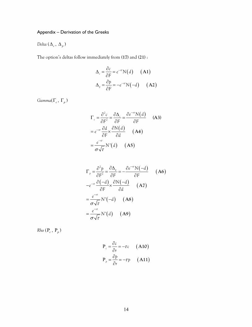
Appendix – Derivation of the Greeks

Delta ( ∆ , ) c p∆

The option’s deltas follow immediately from (17) and (21) :

( ) ( )

( ) (

τ

τ

−

− )

∂∆ = =

∂∂

∆ = = − −∂

rc

rp

ce N d

Fp

e N dF

A1

A2

Gamma( Γ , ) c pΓ

( )

( ) ( )

( ) ( )

τ

τ

τ

σ τ

−

−

−

∂∂ ∂∆Γ = = =

∂ ∂ ∂∂∂

= ×∂ ∂

=

2

2

'

rc

c

r

r

e N dcF F F

N dde

F de

N d

(A3)

A4

A5

( ) ( )

( ) ( ) ( )

( ) ( )

( ) ( )

τ

τ

τ

τ

σ τ

σ τ

−

−

−

−

∂∆ ∂ −∂Γ = = = −

∂ ∂ ∂∂ − ∂ −

− ×∂ ∂

= −

=

2

2

'

'

rp

p

r

r

r

e N dpF F F

d N de

F de

N d

eN d

A6

A7

A8

A9

Rho ( , Ρ ) cΡ p

( )

( )

τ

τ

∂Ρ = = −

∂∂

Ρ = = −∂

c

p

cc

rp

pr

A10

A11

14

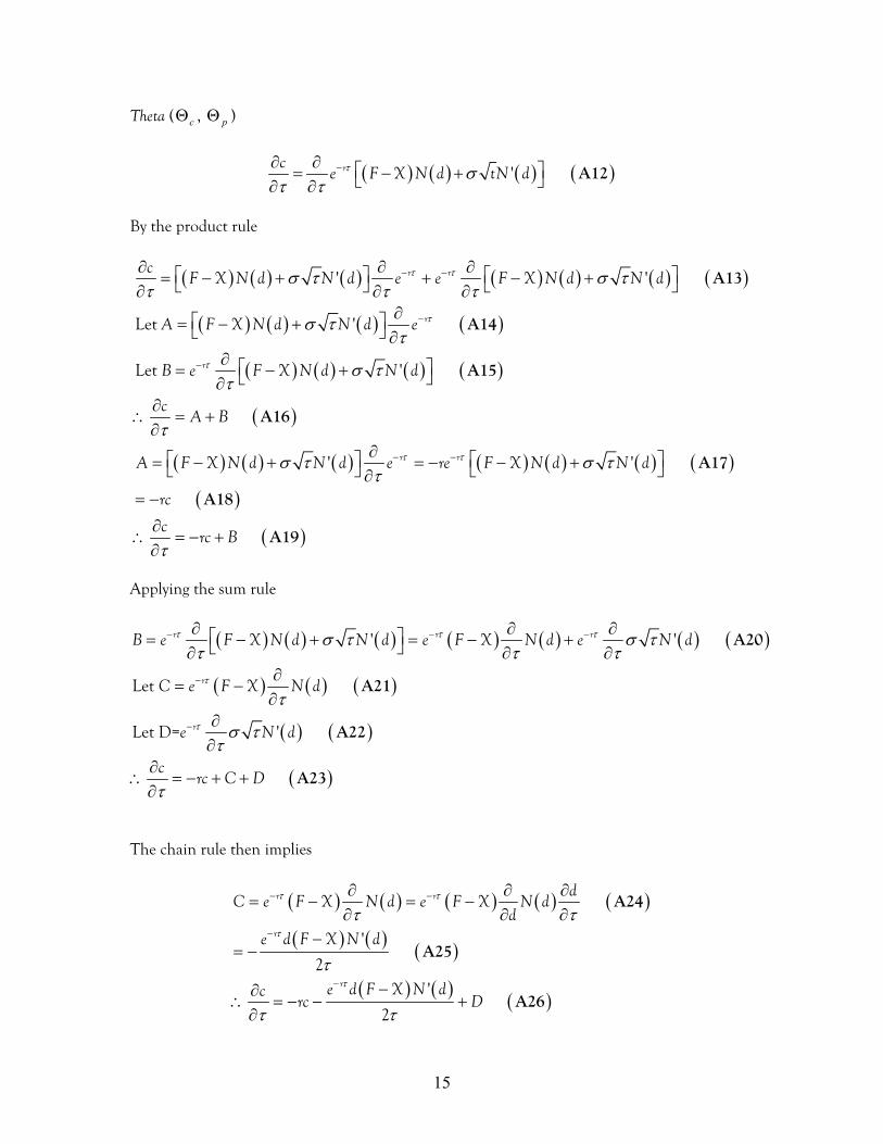
Theta ( Θ , Θ ) c p

( ) ( ) ( ) ( )τ στ τ

−∂ ∂ = − + ∂ ∂' rc

e F X N d tN d A12

By the product rule

( ) ( ) ( ) ( ) ( ) ( ) ( )

( ) ( ) ( ) ( )

( ) ( ) ( ) ( )

( )

( ) ( ) ( ) ( ) ( ) ( )

τ τ

τ

τ

τ τ

σ τ σ ττ τ τ

σ ττ

σ ττ

τ

σ τ σ ττ

− −

−

−

− −

∂ ∂ ∂ = − + + − + ∂ ∂ ∂∂ = − + ∂

∂ = − + ∂∂

∴ = +∂

∂ = − + = − − + ∂

' '

Let '

Let '

' '

r r

r

r

r r

cF X N d N d e e F X N d N d

A F X N d N d e

B e F X N d N d

cA B

A F X N d N d e re F X N d N d

A13

A14

A15

A16

A1( )

( )

( )τ

= −

∂∴ = − +

∂

rc

crc B

7

A18

A19

Applying the sum rule

( ) ( ) ( ) ( ) ( ) ( ) ( )

( ) ( ) ( )

( ) ( )

( )

τ τ τ

τ

τ

σ τ σ ττ τ τ

τ

σ ττ

τ

− − −

−

−

∂ ∂ ∂ = − + = − + ∂ ∂ ∂∂

= −∂

∂∂

∂∴ = − + +

∂

' '

Let

Let D= '

r r r

r

r

B e F X N d N d e F X N d e N d

C e F X N d

e N d

crc C D

A20

A21

A22

A23

The chain rule then implies

( ) ( ) ( ) ( ) ( )

( ) ( ) ( )

( ) ( ) ( )

τ τ

τ

τ

τ τ

τ

τ τ

− −

−

−

∂ ∂ ∂= − = −

∂ ∂ ∂−

= −

−∂∴ = − − +

∂

'

2'

2

r r

r

r

dC e F X N d e F X N d

de d F X N d

e d F X N dcrc D

A24

A25

A26

15

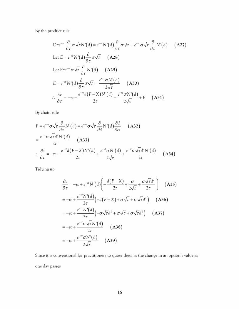
By the product rule

( ) ( ) ( ) ( )

( ) ( )

( ) ( )

( ) ( ) ( )

( ) ( ) ( ) ( )

τ τ τ

τ

τ

ττ

τ τ

σ τ σ τ σ ττ τ τ

σ ττ

σ ττ

σσ τ

τ τσ

τ τ τ

− − −

−

−

−−

− −

∂ ∂ ∂= +

∂ ∂ ∂∂

=∂

∂∂∂

= =∂

−∂∴ = − − + +

∂

D= ' ' '

Let '

Let F= '

''

2

' '

2 2

r r r

r

r

rr

r r

e N d e N d e N d

E e N d

e N d

e N dE e N d

e d F X N d e N dcrc F

A27

A28

A29

A30

A31

By chain rule

( ) ( ) ( )

( ) ( )

( ) ( ) ( ) ( ) ( )

τ τ

τ

τ τ τ

σ τ σ ττ σ

σ ττ

σ σ ττ τ ττ

− −

−

− − −

∂ ∂ ∂= =

∂ ∂ ∂

=

−∂∴ = − − + +

∂

2

2

' '

'

2

' ' '

2 22

r r

r

r r r

dF e N d e N d

d

e d N d

e d F X N d e N d e d N dcrc

A32

A33

A34

Tidying up

( ) ( ) ( )

( ) ( )( ) ( )

( ) ( ) ( )

( ) ( )

( ) ( )

τ

τ

τ

τ

τ

σ σ ττ τ ττ

σ τ σ ττ

σ τ σ τ σ ττ

σ ττ

στ

−

−

−

−

−

−∂= − + − + + ∂

= − + − − + +

= − + − + +

= − +

= − +

2

2

2 2

' 2 22

'

2'

2

'

2'

2

r

r

r

r

r

d F Xc drc e N d

e N drc d F X d

e N drc d d

e N drc

e N drc

A35

A36

A37

A38

A39

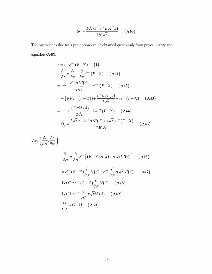
Since it is conventional for practitioners to quote theta as the change in an option’s value as

one day passes

16

( ) ( )ττ στ

−−Θ =

2 '

730

r

c

rc e N dA40

The equivalent value for a put option can be obtained quite easily from put-call parity and

equation (A40).

( ) ( )

( ) ( )

( ) ( ) ( )

( )( ) ( ) ( ) (

( )

)

( ) ( )

( ) ( ) ( )

τ

τ

ττ

ττ τ

ττ

τ τ

τ τ τσ

τσ

τσ

ττ σ τ

τ

−

−

−−

−− −

−−

− −

= − −

∂ ∂ ∂∴ = − −

∂ ∂ ∂

= − + − −

= − + − + − −

= − + − −

− + −∴Θ =

'

2

'

2

'2

2

2 ' 4

730

r

r

rr

rr r

rr

r r

p

p c e F X

p ce F X

e N drc re F X

e N dr p e F X re F X

e N drp re F X

rp e N d re F X

1

A41

A42

A43

A44

A45

Vega σ σ

∂ ∂ ∂ ∂

,c p

( ) ( ) ( ) ( )τ σ τσ σ

−∂ ∂ = − + ∂ ∂' rc

e F X N d N d A46

( ) ( ) ( ) ( )

( ) ( ) ( )

( ) ( )

( )

τ τ

τ

τ

σ τσ σ

σ

σ τσ

σ

− −

−

−

∂ ∂= − +

∂ ∂∂

−∂

∂∂

∂= +

∂

'

Let G =

Let H = '

r r

r

r

e F X N d e N d

e F X N d

e N d

cG H

A47

A48

A49

A50

17

By the chain rule

( ) ( ) ( ) ( ) ( )

( ) ( ) ( )

( ) ( )

τ τ

τ

τ

σ σ

στ

− −

−

−

∂ ∂ ∂= − = −

∂ ∂ ∂− −

=

= − 2

'

'

r r

r

r

dG e F X N d e F X N d

de d F X N d

e d N d

A52

A53

A54

By the product and chain rules

( ) ( ) ( ) ( )

( ) ( ) ( )

( ) ( ) ( )

( ) ( ) ( ) ( )

( ) ( )

τ τ τ

τ τ

τ

τ τ

τ

σ τ σ τ σ τσ σ

τ σ τσ

τ

τ τσ

τ

− − −

− −

−

− −

−

∂ ∂ ∂ ∂= +

∂ ∂ ∂ ∂

= +

= +

∂

σ

∴ = + −∂

=

2

2

2 2

H = ' ' '

' '

1 '

1 ' '

'

r r r

r r

r

r r

r

de N d e N d e N d

dd

e N d e N d

e d N d

ce d N d e d N d

e N d

A55

A56

A57

A58

A59

Since practitioners generally present vega in terms of a one percentage point change in

volatility, we present vega here as

( ) ( )τ τ

σ

−∂=

∂'

100

re N dcA60

Put-call parity shows that the vega of a put option equals the vega of a call option.

( ) ( )

( ) ( )

τ

τ

σ σ σ σ

−

−

= − −

∂ ∂ ∂ ∂∴ = − −

∂ ∂ ∂ ∂

=

r

r

p c e F X

p c ce F X

1

A61 QED

18

References Bachelier, Louis. (1900) Théorie de la Spéculation. Paris: Gauthier-Villars. Black, Fischer, [1976]. “The Pricing of Commodity Options.” Journal of Financial Economics, 3: 167 – 179. Black, Fischer and Myron Scholes, [1973]. “The Pricing of Options and Corporate Liabilities.” Journal of Political Economy. 81: 637 - 654. Cox, John C. and Stephen A. Ross, [1976]. “The Valuation of Options for Alternative Stochastic Processes.” Journal of Financial Economics. 3: 145 – 166. Dawson, Paul, David Blake, Andrew J G Cairns and Kevin Dowd, [2007]. “Completing the Market for Survivor Derivatives.” Working Paper. Dowd, Kevin, [2005]. Measuring Market Risk. Second edition. John Wiley. Dowd, Kevin, Andrew J G Cairns, David Blake and Paul Dawson, [2006]. “Survivor Swaptions.” Journal of Risk and Insurance. 73: 1 – 17. Merton, Robert C., [1973]. “Theory of Rational Option Pricing.” Bell Journal of Economics and Management Science. 4: 141 – 183. Rubinstein, Mark, [1994]. “Implied Binomial Trees.” Journal of Finance. 49: 771 – 818. Stoll, Hans, [1969]. “The Relationship between Put and Call Option Prices.” Journal of Finance. 14: 319 – 332.

19

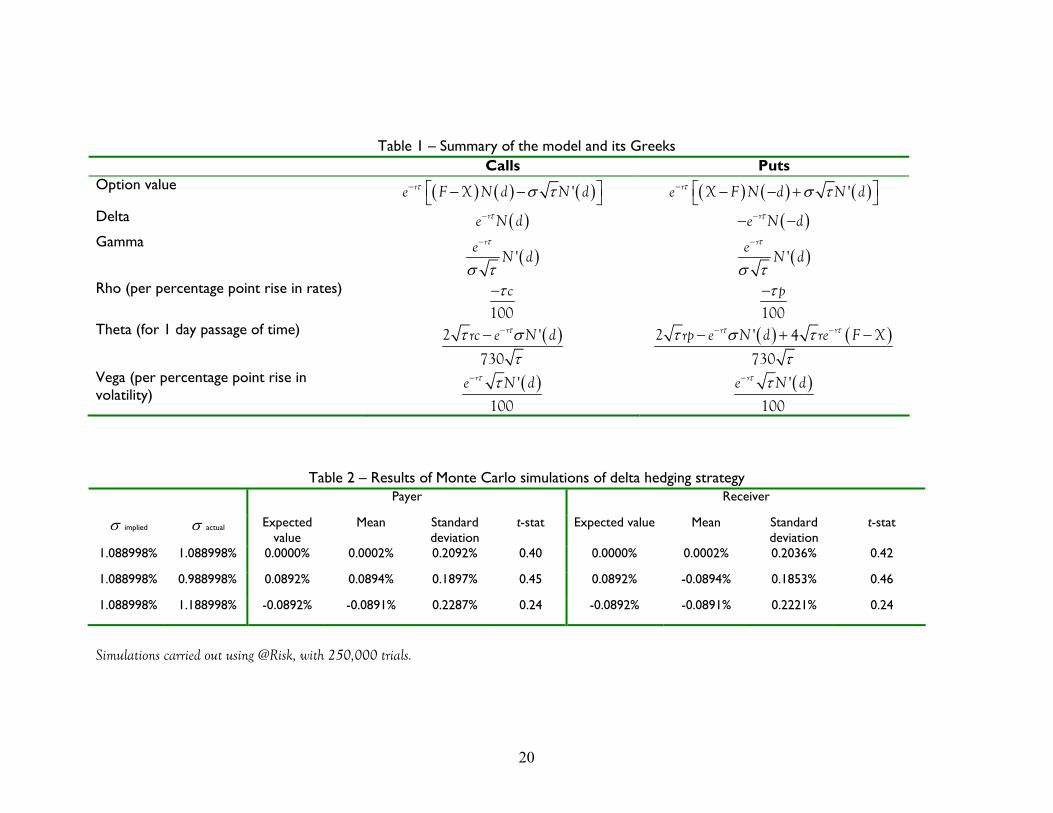
Table 1 – Summary of the model and its Greeks

Calls Puts Option value ( ) ( ) ( )τ σ τ− − − 're F X N d N d ( ) ( ) ( )τ σ τ− − − + 're X F N d N d

Delta ( )τ− re N d ( )τ−− −re N d Gamma

( )τ

σ τ

−

're

N d ( )τ

σ τ

−

're

N d

Rho (per percentage point rise in rates) τ−100

c

τ−100

p

Theta (for 1 day passage of time) ( )ττ στ

−−2 '

730

rrc e N d

( ) ( )τ ττ σ ττ

− −− + −2 ' 4

730

r rrp e N d re F X

Vega (per percentage point rise in volatility)

( )τ τ− '

100

re N d

( )τ τ− '

100

re N d

Table 2 – Results of Monte Carlo simulations of delta hedging strategy

Payer Receiver

σ implied σ actual Expected value

Mean Standarddeviation

t-stat Expected value Mean Standarddeviation

t-stat

1.088998% 1.088998% 0.0000% 0.0002% 0.2092% 0.40 0.0000% 0.0002% 0.2036% 0.42

1.088998% 0.988998% 0.0892% 0.0894% 0.1897% 0.45 0.0892% -0.0894% 0.1853% 0.46

1.088998% 1.188998% -0.0892% -0.0891% 0.2287% 0.24 -0.0892% -0.0891% 0.2221% 0.24

Simulations carried out using @Risk, with 250,000 trials.

20