This content has been downloaded from IOPscience. Please scroll down to see the full text.

Download details:

IP Address: 134.153.184.170

This content was downloaded on 01/08/2014 at 13:12

Please note that terms and conditions apply.

Opto- and electro-mechanical entanglement improved by modulation

View the table of contents for this issue, or go to the journal homepage for more

2012 New J. Phys. 14 075014

(http://iopscience.iop.org/1367-2630/14/7/075014)

Home Search Collections Journals About Contact us My IOPscience

T h e o p e n – a c c e s s j o u r n a l f o r p h y s i c s

New Journal of Physics

Opto- and electro-mechanical entanglementimproved by modulation

A Mari1,2 and J Eisert1,2,3

1 Dahlem Center for Complex Quantum Systems, Freie Universitat Berlin,14195 Berlin, Germany2 Institute of Physics and Astronomy, University of Potsdam, D-14476 Potsdam,GermanyE-mail: jense@physik.fu-berlin.de

New Journal of Physics 14 (2012) 075014 (12pp)Received 7 February 2012Published 19 July 2012Online at http://www.njp.org/doi:10.1088/1367-2630/14/7/075014

Abstract. One of the main milestones in the study of opto- and electro-mechanical systems is to certify entanglement between a mechanical resonatorand an optical or microwave mode of a cavity field. In this work, we showhow a suitable time-periodic modulation can help to achieve large degrees ofentanglement, building upon the framework introduced in Mari and Eisert (2009Phys. Rev. Lett. 103 213603). It is demonstrated that with suitable driving,the maximum degree of entanglement can be significantly enhanced, in a wayexhibiting a nontrivial dependence on the specifics of the modulation. Such time-dependent driving might help to experimentally achieve entangled mechanicalsystems also in situations when quantum correlations are otherwise suppressedby thermal noise.

3 Author to whom any correspondence should be addressed.

New Journal of Physics 14 (2012) 0750141367-2630/12/075014+12$33.00 © IOP Publishing Ltd and Deutsche Physikalische Gesellschaft

2

Contents

1. Introduction 22. Modulated opto- and electro-mechanical systems 33. Classical periodic orbits: first moments 44. Quantum correlations: second moments 45. Entanglement resonances 66. Opto- and electro-mechanical entanglement in realistic settings 87. Summary 10Acknowledgments 10Appendix 10References 11

1. Introduction

Opto-mechanical [1–7] and electro-mechanical systems [8–13] are promising candidates forrealizing architectures exhibiting quantum behavior in macroscopic structures. Once thequantum regime is reached, exciting applications in quantum technologies such as realizingprecise force sensors are conceivable [15, 16]. One of the requirements to render such anapproach feasible, needless to say, is to be able to certify that a mechanical degree of freedom isdeeply in the quantum regime [16–20]. The detection of entanglement arguably constitutes theultimate benchmark in this respect. While effective ground state cooling has indeed been closelyapproached experimentally [6, 10] and achieved [7, 9, 13], the detection of entanglement is stillin progress.

In this paper, we emphasize that a mere suitable time modulation of the driving field maysignificantly help to achieve entanglement between a mechanical mode and a radiation mode ofthe system. We extend the idea of [21], putting emphasis on the improvement of entanglementby means of suitable modulations [21–23]. This time dependence of the driving indirectlyaffects the effective radiation pressure coupling between the two modes and generates non-trivial entanglement resonances. In comparison with single-mode squeezing, which is the mainsubject of [21], here we show that two-mode squeezing is optimized at different modulationfrequencies related to the normal mode splitting of the system.

Several other schemes have been proposed in the literature for squeezing or entangling amechanical mode with an optical or microwave field. These are based on driving one singlesideband [14, 19, 20, 30], driving two sidebands with the same power [23], driving twoindependent modes of the cavity [29] and directly modulating the frequencies of the modes(parametric amplification) [22]. In our system, a single cavity mode is externally driven witha red-detuned main carrier and modulated with a weak blue sideband tuned at particularresonance frequencies. In this way, the system is stable and with the appropriate choice of thedriving pattern, large degrees of two-mode squeezing can be reached. Moreover, in our scheme,entanglement appears in the long time limit as a stationary property without the need for anypost-selection of the state conditioned on external measurement results.

The body of the paper is organized into four sections. In the first two sections the classicaldynamics of the system and its quantum fluctuations are studied in a very general framework.

New Journal of Physics 14 (2012) 075014 (http://www.njp.org/)

3

In the third section, we focus on the main result of the paper: the appearance of entanglementresonances for particular choices of the modulation frequencies. In section 4, this resonancephenomenon is applied to two examples of opto- and electro-mechanical systems, whoseparameters have been realistically chosen in agreement with recent experiments.

2. Modulated opto- and electro-mechanical systems

We consider the simplest scenario of a mechanical resonator of frequency ωm coupled to a singlemode of the electromagnetic field of frequency ωa. This radiation field could be an opticalmode of a Fabry–Perot cavity [1–7, 18, 19, 24] or a microwave mode of a superconductivecircuit [8–10, 14]. It can be shown that the Hamiltonians associated with this two experimentalsettings are formally equivalent [14, 19] and therefore the theory that we are going to introduceis general enough to describe both types of systems.

We assume that the radiation mode is driven by a coherent field with a time-dependentamplitude E(t) and frequency ωl . The particular choice of the time dependence is leftunspecified but we impose the structure of a periodic modulation such that E(t + τ) = E(t)for some τ > 0 of the order of ω−1

m . In this sense, the driving regime that we are going to studyis intermediate between the two opposite extremes of constant amplitude and short pulses. TheHamiltonian of the system is

H = hωaa†a + 12 hωm(p2 + q2) − hga†aq + ih[E(t)e−iωl ta†

− E∗(t)eiωl ta], (1)

where the mechanical mode is described in terms of dimensionless position and momentumoperators satisfying [q, p] = i , while the radiation mode is captured by creation and annihilationoperators obeying the bosonic commutation rule [a, a†] = 1. The two modes interact via aradiation pressure potential with a strength given by the coupling parameter g.

In addition to this coherent dynamics, the mechanical mode will be unavoidably damped ata rate γm, while the optical/microwave mode will decay at a rate κ . These dissipative processesand the associated fluctuations can be taken into account in the Heisenberg picture by thefollowing set of quantum Langevin equations [14, 17–19]:

q = ωm p,

p = − ωmq − γm p + ga†a + ξ, (2)

a = − (κ + i1)a + igaq + E(t) +√

2κain.

In this set of equations a convenient rotating frame has been chosen a 7→ a e−iωl t , such thatthe detuning parameter is 1 = ωa − ωl . The operators ξ and ain represent the mechanical andoptical bath operators respectively, and their correlation functions are well approximated bydelta functions

〈ξ(t)ξ(t ′) + ξ(t ′)ξ(t)〉/2 = γm(2nm + 1)δ(t − t ′),

〈ain(t)ain†(t ′)〉 = (na + 1)δ(t − t ′), (3)

〈ain†(t)ain(t ′)〉 = naδ(t − t ′),

where nx = (exp(hωx/(kB T )) − 1)−1, is the bosonic mean occupation number at temperature T .

New Journal of Physics 14 (2012) 075014 (http://www.njp.org/)

4

3. Classical periodic orbits: first moments

We are interested in the coherent strong driving regime when 〈a〉 � 1. In this limit, thesemiclassical approximations 〈a†a〉 ' |〈a〉|

2 and 〈aq〉 ' 〈a〉〈q〉 are good approximations.Within this approximation, one can average both sides of equation (2) and get a differentialequation for the first moments of the canonical coordinates

〈q〉 = ωm〈p〉,

〈 p〉 = − ωm〈q〉 − γm〈p〉 + g|〈a〉|2, (4)

〈a〉 = − (κ + i1)〈a〉 + ig〈a〉〈q〉 + E(t).

Far away from the well known opto- and electro-mechanical instabilities, asymptoticτ -periodic solutions can be used as ansatze for equation (4) (see the appendix for a moredetailed analysis). These solutions represent periodic orbits in phase space and are usuallycalled the limit cycles. These cycles are induced by modulation and should not be confusedwith the limit cycles emerging in the strong driving regime due to the nonlinearity of thesystem. Because of the asymptotic periodicity of the solutions, one can define the fundamentalmodulation frequency as � = 2p/s, such that each periodic solution can be expanded in thefollowing Fourier series

〈O(t)〉 =

∞∑n=−∞

On ein�t , O = q, p, a. (5)

The Fourier coefficients {On} appearing in equation (5) can be analytically estimated as shownin the appendix and they completely characterize the classical asymptotic dynamics of thesystem.

Finally we note that the classical evolution of the dynamical variables will shift thedetuning to the effective value of 1(t) = 1 − g〈q(t)〉. For the same reason, it is also convenientto introduce an effective coupling constant defined as

g(t) =√

2g〈a(t)〉. (6)

4. Quantum correlations: second moments

The classical limit cycles are given by the asymptotic solutions of equation (4). In order tocapture the quantum fluctuations around the classical orbits, we introduce a column vector ofnew quadrature operators u = [δq, δp, δx, δy]T defined as:

δq = q − 〈q(t)〉,

δp = p − 〈p(t)〉,

δx =[(a − 〈a(t)〉) + (a − 〈a(t)〉)†

]/√

2,

δy = −i[(a − 〈a(t)〉) − (a − 〈a(t)〉)†

]/√

2.

(7)

This set of canonical coordinates can be viewed as describing a time-dependent reference frameco-moving with the classical orbits. The corresponding vector of noise operators will be

n = [0, ξ, (ain + ain†)/√

2, −i(ain− ain†)/

√2]T. (8)

New Journal of Physics 14 (2012) 075014 (http://www.njp.org/)

5

Since we are in the limit in which classical orbits emerge (〈a〉 � 1), it is a reasonableapproximation to express the previous set of Langevin equations (2) in terms of the newfluctuation operators (7) and neglect all their quadratic powers. The resulting linearized systemcan be written as a matrix equation [21],

u = A(t)u + n(t), (9)

where

A(t) =

0 ωm 0 0

−ωm −γm <g(t) =g(t)−=g(t) 0 −κ 1(t)<g(t) 0 −1(t) −κ

(10)

is a real time-dependent matrix.If the system is stable, and as long as the linearization is valid, the quantum state of the

system will converge to a Gaussian state with time-dependent first and second moments. Thefirst moments of the state correspond to the classical limit cycles introduced in the previoussection. The second moments can be expressed in terms of the covariance matrix V (t) withentries

Vk,l(t) = 〈uk(t)u†l (t) + u†

l (t)uk(t)〉/2. (11)

One can also define a diffusion matrix D as

δ(t − t ′)Dk,l = 〈nk(t)n†l (t

′) + n†l (t

′)nk(t)〉/2, (12)

which, from the properties of the bath operators (4), is diagonal and equal to

D = diag[0, γ (2nm + 1), κ(2na + 1), κ(2na + 1)]. (13)

From equations (9) and (12), one can easily derive a linear differential equation for thecorrelation matrix,

d

dtV (t) = A(t)V (t) + V (t)AT(t) + D. (14)

Since the first and second moments are specified, equations (4) and (14) provide a completedescription of the asymptotic dynamics of the system. Apart from the linearization aroundclassical cycles, no further approximation has been done: neither a weak coupling, adiabaticnon rotating-wave approximation. Numerical solutions of both equations (4) and (14) can bestraightforwardly found. These solutions will be used to calculate the exact amount of opto- andelectro-mechanical entanglement present in the system.

The asymptotic periodicity of the classical solutions (equation (5)) implies that, in the longtime limit, A(t + τ) = A(t). This means that equation (14) is a linear differential equation withperiodic coefficients and then all the machinery of Floquet theory is in principle applicable.Here, however, since we are only interested in asymptotic solutions, we are not going to studyall the Floquet exponents of the system. The only property that we need is that, in the long timelimit, stable solutions will acquire the same periodicity of the coefficients:

V (t + τ) = V (t). (15)

This is a simple corollary of Floquet’s theorem. In the subsequent sections we will apply theprevious theory to some particular experimental setting and show how a simple modulationof the driving field can significantly improve the amount of opto- and electro-mechanicalentanglement.

New Journal of Physics 14 (2012) 075014 (http://www.njp.org/)

6

5. Entanglement resonances

In this section, we are going to study what kind of amplitude modulation is optimal forgenerating entanglement between the radiation and mechanical modes. As a measure ofentanglement we use the logarithmic negativity EN which, since the state is Gaussian, can beeasily computed directly from the correlation matrix V (t) [26–28]. We have also seen that thecorrelation matrix is, in the long time limit, τ -periodic. This suggests that it is sufficient to studythe variation of entanglement in a finite interval of time [t, t + τ ] for large times t . One can thendefine the maximum amount of achievable entanglement as

EN = limt→∞

maxh∈[t,t+τ ]

EN(h). (16)

This will be the quantity that we are going to optimize.We first study a very simple set of parameters (see caption of figure 1) in order to

understand what the optimal choice is for the modulation frequency. For this purpose, we imposeeffective coupling to have this simple structure

g(t) = g0 + g� e−i�t , (17)

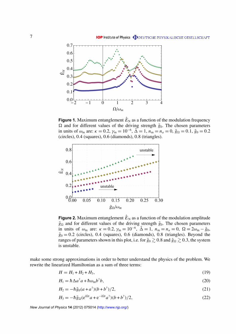
where g0 is associated with the main driving field with detuning 1, while g� is the amplitudeof a further sideband shifted by a frequency � from the main carrier. Without loss of generalitywe will assume g0 and g� to be positive reals. This kind of driving is a natural one and it hasbeen chosen for reasons that will become clear later. From now on we set the detuning of thecarrier frequency to be equal to the mechanical frequency 1 = ωm. This choice of the detuningcorresponds to the well-known sideband cooling setting [17, 24] and it has been shown to bealso optimal for maximizing opto-mechanical entanglement with a non-modulated driving [19].Figure 1 shows the maximum entanglement EN between the mechanical and the radiation modesas a function of the modulation frequency � and for different values of the driving amplitudeg0. This maximum degree of entanglement has been calculated for t > 200/κ , when the systemhas well reached its periodic steady state.

We observe that in figure 1 there are two main resonant peaks at the modulation frequencies

� ' 2ωm ± g0, (18)

that we are going to carefully explain later. Note also that, if compared to [21], the choices ofmodulations that give rise to the optimal local single-mode squeezing of the mechanical mode(� = 2ωm) and the degree of entanglement (� = 2ωm ± g0) are not identical. This is rootedin the ‘monogamous nature’ of squeezing: For a fixed spectrum of the covariance matrix, onecan either have large local or two-mode squeezing. In figure 1 we also observe that the heightof the two peaks, due to cavity filtering, is not equal: the first resonance at � = 2ωm − g0 isbetter for the amount of steady state entanglement. One could also ask what the behavior ofentanglement is when we change the amplitude of the modulation. Figure 2 shows the amountof entanglement EN as a function of g� and for different choices of g0. We observe thatentanglement is monotonically increasing in g� up to a threshold where the system becomesunstable.

We will now provide some intuition on why one should expect the main resonances at thelocations where they are observed. The exact dynamics of the linearized system can be studiedvia equation (9). This is how figures 1 and 2 were generated. Now, however, we are going to

New Journal of Physics 14 (2012) 075014 (http://www.njp.org/)

7

Figure 1. Maximum entanglement EN as a function of the modulation frequency� and for different values of the driving strength g0. The chosen parametersin units of ωm are: κ = 0.2, γm = 10−6, 1 = 1, nm = na = 0, g� = 0.1, g0 = 0.2(circles), 0.4 (squares), 0.6 (diamonds), 0.8 (triangles).

Figure 2. Maximum entanglement EN as a function of the modulation amplitudeg� and for different values of the driving strength g0. The chosen parametersin units of ωm are: κ = 0.2, γm = 10−6, 1 = 1, nm = na = 0, � = 2ωm − g0,g0 = 0.2 (circles), 0.4 (squares), 0.6 (diamonds), 0.8 (triangles). Beyond theranges of parameters shown in this plot, i.e. for g0 & 0.8 and g� & 0.3, the systemis unstable.

make some strong approximations in order to better understand the physics of the problem. Werewrite the linearized Hamiltonian as a sum of three terms:

H = H1 + H2 + H3, (19)

H1 = h1a†a + hωmb†b, (20)

H2 = −hg0(a + a†)(b + b†)/2, (21)

H3 = −hg�(ei�ta + e−i�ta†)(b + b†)/2, (22)

New Journal of Physics 14 (2012) 075014 (http://www.njp.org/)

8

where the new bosonic operators a = (δx + iδy)/√

2 and b = (δq + iδp)/√

2 are defined withrespect to fluctuation quadratures. The three terms H1, H2 and H3 correspond to free evolution,the driving carrier and the weak modulation sideband respectively. We assume the modulationterm H3 to be a weak ‘perturbation of the perturbation’ H2. In other words we take twohierarchic limits ω � g0 � g� that will allow us to perform two successive rotating waveapproximations: first with respect to H1 and then with respect to H2. In interaction picture withrespect to H1 and remembering that we fixed 1 = ωm, we get:

H ′

2 ' −hg0(ab† + a†b)/2, (23)

H ′

3 ' −hg�(ei(�−2ωm)tab + e−i(�−2ωm)ta†b†)/2. (24)

In the first equation, we neglected all rotating terms while in the second we neglected the termproportional to ei�tab† + e−i�ta†b because it is resonant only in the trivial case of � = 0 andproduces only a renormalization of g0. Now we apply the following Bogoliubov transformation

c± = (a ± b)/√

2. (25)

These new bosonic operators describe the well known hybridization of the system into normalmodes as described in [5, 25]. In this canonical frame H ′

2 is diagonal and we get:

H ′

2 ' −hgo(c†+c+ − c†

−c−)/2, (26)

H ′

3 ' −hg� ei(�−2ωm)t(c+c+ + c−c−)/2 + h.c. (27)

We are finally ready to perform a second rotating wave approximation, which is valid in theweak modulation limit g0 � g�. In interaction picture with respect to H ′

2 we obtain

H ′′

3 ' −hg� ei(�−2ωm)t(eig0tc+c+ + e−ig0tc−c−)/2 + h.c. (28)

From the structure of equation (28) we observe that there are two resonances � = 2ωm ± gassociated with the two distinct squeezing interactions

H± = −hg�(c∓c∓ + c†∓

c†∓)/2. (29)

Because of equation (25), squeezing of one of the hybrid modes implies that one of theEinstein–Podolsky–Rosen (EPR) variances is reduced below the uncertainty of the vacuumfluctuations. This suggests the presence of entanglement. Actually, bosonic modes with EPRcorrelations are the most relevant and paradigmatic example of entangled states and they are thebasis of many quantum information protocols [26].

6. Opto- and electro-mechanical entanglement in realistic settings

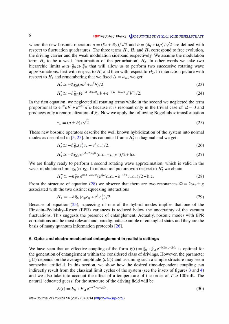
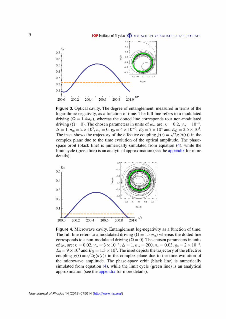
We have seen that an effective coupling of the form g(t) = g0 + g� e−i(2ωm−g0)t is optimal forthe generation of entanglement within the considered class of drivings. However, the parameterg(t) depends on the average amplitude 〈a(t)〉 and assuming such a simple structure may seemsomewhat artificial. In this section, we show how the desired time-dependent coupling canindirectly result from the classical limit cycles of the system (see the insets of figures 3 and 4)and we also take into account the effect of a temperature of the order of T ' 100 mK. Thenatural ‘educated guess’ for the structure of the driving field will be

E(t) = E0 + E� e−i(2ωm−g0)t . (30)

New Journal of Physics 14 (2012) 075014 (http://www.njp.org/)

9

Figure 3. Optical cavity. The degree of entanglement, measured in terms of thelogarithmic negativity, as a function of time. The full line refers to a modulateddriving (� = 1.4ωm), whereas the dotted line corresponds to a non-modulateddriving (� = 0). The chosen parameters in units of ωm are: κ = 0.2, γm = 10−6,1 = 1, nm = 2 × 103, na = 0, g0 = 4 × 10−6, E0 = 7 × 104 and E� = 2.5 × 104.The inset shows the trajectory of the effective coupling g(t) =

√2g〈a(t)〉 in the

complex plane due to the time evolution of the optical amplitude. The phase-space orbit (black line) is numerically simulated from equation (4), while thelimit cycle (green line) is an analytical approximation (see the appendix for moredetails).

Figure 4. Microwave cavity. Entanglement log-negativity as a function of time.The full line refers to a modulated driving (� = 1.3ωm) whereas the dotted linecorresponds to a non-modulated driving (� = 0). The chosen parameters in unitsof ωm are: κ = 0.02, γm = 3 × 10−6, 1 = 1, nm = 200, na = 0.03, g0 = 2 × 10−5,E0 = 9 × 103 and E� = 1.3 × 103. The inset depicts the trajectory of the effectivecoupling g(t) =

√2g〈a(t)〉 in the complex plane due to the time evolution of

the microwave amplitude. The phase-space orbit (black line) is numericallysimulated from equation (4), while the limit cycle (green line) is an analyticalapproximation (see the appendix for more details).

New Journal of Physics 14 (2012) 075014 (http://www.njp.org/)

10

For the choice of the other parameters, we focus on two sets of parameters corresponding totwo completely different systems: an optical cavity with a moving mirror and a superconductingwave guide coupled to a mechanical resonator. The parameters are chosen according to realisticexperimental settings; see, e.g. [5] (opto-mechanical system) and [9] (electro-mechanicalsystem). Figures 3 and 4 show that, in both experimental scenarios, entanglement cansignificantly be increased by an appropriate modulation of the driving field.

7. Summary

In this paper, we have shown how time-modulation can significantly enhance the maximumdegree of entanglement. Triggered by the time-modulated driving, the mode of theelectromechanical field as well as the mechanical mode start ‘rotating around each other’in a complex fashion, giving rise to increased degrees of entanglement. The dependence onfrequencies of the additional modulation is intricate, with resonances greatly improving theamount of entanglement that can be reached. The ideas presented here could be particularlybeneficial for preparing systems in entangled states in the first place, in scenarios where theparameters are such that the states prepared are close to the boundary to entangled states, butwhere this boundary is otherwise not yet quite reachable with the present technology. At thesame time, such ideas are expected to be useful in metrological applications whenever highdegrees of entanglement are needed.

Acknowledgments

We thank the EU (MINOS, COMPAS, QESSENCE) and the BMBF (QuOReP) for support.

Appendix

In this appendix, we derive analytical formulas for the asymptotic solutions of the classicalsystem of dynamical equation (4). A crucial assumption for the following procedure is that it ispossible to expand the solutions in powers of the coupling constant g

〈O〉(t) =

∞∑j=0

O j(t)gj , (A.1)

where O = a, p, q. This is justified only if the system is far away from multi-stabilities andthe radiation pressure coupling can be treated in a perturbative way. A very important featureof the set of equation (4) is that they contain only two nonlinear terms and those terms areproportional to the coupling parameter g. This implies that, if we use the ansatz (A.1), eachfunction O j will be a solution of linear differential equation with time dependent parametersdepending on the previous solution O j−1(t). Since E(t) = E(t + τ), from a recursive applicationof Floquet’s theorem, follows that stable solutions will converge to periodic limit cycles havingthe same periodicity of driving: 〈O(t)〉 = 〈O(t + s)〉. One can exploit this property and performa double expansion in powers of g and in terms of Fourier components

〈O〉(t) =

∞∑j=0

∞∑n=−∞

On, j ein�t g j , (A.2)

New Journal of Physics 14 (2012) 075014 (http://www.njp.org/)

11

where n are integers and � = 2π/τ . A similar Fourier series can be written for the periodicdriving field,

E(t) =

∞∑n=−∞

ENein�t . (A.3)

The coefficients On, j can be found by direct substitution in equation (4). They are completelydetermined by the following set of recursive relations:

qn,0 = pn,0 = 0, an,0 =E−n

κ + i(1 + n�), (A.4)

corresponding to the 0-order perturbation with respect to g, and

pn, j =in�

ωmqn, j , (A.5)

qn, j = ωm

j−1∑k=0

∞∑m=−∞

a∗

m,k an+m, j−k−1

ω2m − n�2 + iγmn�

, (A.6)

an, j = ij−1∑k=0

∞∑m=−∞

am,kqn−m, j−k−1

κ + i(1 + n�), (A.7)

giving all the j-order coefficients in a recursive way. For all the examples analyzed in this paper,we truncated the analytical solutions up to j 6 3 and |n|6 2. This level of approximation isalready high enough to reproduce the exact numerical solutions well.

References

[1] Gigan S, Bohm H R, Paternostro M, Blaser F, Langer G, Hertzberg J B, Schwab K, Baeuerle D, AspelmeyerM and Zeilinger A 2006 Nature 444 67

[2] Arcizet O, Cohadon P-F, Briant T, Pinard M and Heidmann A 2006 Nature 444 71[3] Kleckner D and Bouwmeester D 2006 Nature 444 75[4] Schliesser A, Del’Haye P, Nooshi N, Vahala K J and Kippenberg T J 2006 Phys. Rev. Lett. 97 243905[5] Groblacher S, Hammerer K, Vanner M R and Aspelmeyer M 2009 Nature 460 724[6] Riviere R, Deleglise S, Weis S, Gavartin E, Arcizet O, Schliesser A and Kippenberg T J 2011 Phys. Rev. A

83 063835[7] Chan J, Mayer Alegre T P, Safavi-Naeini A H, Hill J T, Krause A, Groeblacher S, Aspelmeyer M

and Painter O 2011 Nature 478 89[8] Teufel J D, Harlow J W, Regal C A and Lehnert K W 2008 Phys. Rev. Lett. 101 197203[9] Teufel J D, Donner T, Li D, Harlow J H, Allman M S, Cicak K, Sirois A J, Whittaker J D, Lehnert K W and

Simmonds R W 2011 Nature 475 359[10] Rocheleau T, Ndukum T, Macklin C, Hertzberg J B, Clerk A A and Schwab K C 2010 Nature 463 72[11] LaHaye M D, Buu O, Camarota B and Schwab K C 2004 Science 304 74[12] Knobel R G and Cleland A N 2003 Nature 424 291[13] Connell A D O et al 2010 Nature 464 697[14] Vitali D, Tombesi P, Woolley M J, Doherty A C and Milburn G J 2007 Phys. Rev. A 76 042336[15] Schwab K C and Roukes M L 2005 Phys. Today 58 36[16] Marquardt F and Girvin S M 2009 Physics 2 40[17] Aspelmeyer M 2010 Nature 464 685

New Journal of Physics 14 (2012) 075014 (http://www.njp.org/)

12

[18] Paternostro M, Vitali D, Gigan S, Kim M S, Brukner C, Eisert J and Aspelmeyer M 2007 Phys. Rev. Lett.99 250401

[19] Vitali D, Gigan S, Ferreira A, Bohm H R, Tombesi P, Guerreiro A, Vedral V, Zeilinger A and Aspelmeyer M2007 Phys. Rev. Lett. 98 030405

[20] Eisert J, Plenio M B, Bose S and Hartley J 2004 Phys. Rev. Lett. 93 190402[21] Mari A and Eisert J 2009 Phys. Rev. Lett. 103 213603[22] Woolley M J, Doherty A C, Milburn G J and Schwab K C 2008 Phys. Rev. A 78 062303[23] Clerk A A, Marquardt F and Jacobs K 2008 New J. Phys. 10 095010[24] Marquardt F, Chen J P, Clerk A A and Girvin S M 2007 Phys. Rev. Lett. 99 093902[25] Dobrindt J M, Wilson-Rae I and Kippenberg T J 2008 Phys. Rev. Lett. 101 263602[26] Eisert J 2001 PhD Thesis University of Potsdam (arXiv:quant-ph/0610253)

Eisert J and Plenio M B 1999 J. Mod. Opt. 46 145[27] Vidal G and Werner R F 2002 Phys. Rev. A 65 032314[28] Plenio M B 2005 Phys. Rev. Lett. 95 090503[29] Genes C, Mari A, Vitali D and Tombesi P 2009 Adv. At. Mol. Opt. Phys. 57 33-86[30] Tian L, Allman M S and Simmonds R W 2008 New J. Phys. 10 115001

New Journal of Physics 14 (2012) 075014 (http://www.njp.org/)