OR-Gym: A Reinforcement Learning Library for Operations

Submitted to INFORMS Journal on Computingmanuscript (Please, provide the manuscript number!)

Authors are encouraged to submit new papers to INFORMS journals by means ofa style file template, which includes the journal title. However, use of a templatedoes not certify that the paper has been accepted for publication in the named jour-nal. INFORMS journal templates are for the exclusive purpose of submitting to anINFORMS journal and should not be used to distribute the papers in print or onlineor to submit the papers to another publication.

OR-Gym: A Reinforcement Learning Library forOperations Research Problems

Christian D. Hubbs, Hector D. Perez, Owais Sarwar, Ignacio E. GrossmannDepartment of Chemical Engineering, Carnegie Mellon University, Pittsburgh, PA 15213

[email protected], [email protected], [email protected], [email protected]

Nikolaos V. SahinidisH. Milton Stewart School of Industrial & Systems Engineering and School of Chemical & Biomolecular Engineering, Georgia

Institute of Technology, Atlanta, GA 30332, [email protected]

John M. WassickDow Chemical, Digital Fulfillment Center, Midland, MI 48667

[email protected]

Reinforcement learning (RL) has been widely applied to game-playing and surpassed the best human-level

performance in many domains, yet there are few use-cases in industrial or commercial settings. In this

work, we introduce OR-Gym, an open-source library for developing reinforcement learning algorithms to

address operations research problems. We provide benchmarks for a selection of problems–the knapsack,

multi-dimensional bin packing, multi-echelon inventory management, and multi-period asset allocation

problems–using both reinforcement learning and classical operations research models. These problems are

used in logistics, finance, engineering, and are common in many business operation settings. We develop

environments based on prototypical models in the literature and implement various optimization and heuristic

models in order to benchmark the RL results. Given the differences between RL and classical modeling

paradigms, we provide descriptions of design decisions in order to give readers insight into applying these

techniques to additional problems and where it may or may not be appropriate. By re-framing a series

of classic optimization problems as RL tasks, we seek to provide a new tool for the operations research

community, while also opening those in the RL community to many of the problems and challenges in the OR

field. Through the experimental results, we show that RL provides a promising alternative to many existing

methods for addressing optimization problems under uncertainty.

Key words : Machine Learning, Reinforcement Learning, Operations Research

1

Hubbs et al.: OR-Gym: A Reinforcement Learning Library2 Article submitted to INFORMS Journal on Computing; manuscript no. (Please, provide the manuscript number!)

1. Introduction

Reinforcement learning (RL) is a branch of machine learning that seeks to make a series of

sequential decisions to maximize a reward. The technique has received widespread attention

in game-playing, whereby RL approaches have beaten some of the world’s best human

players in domains such as Go and DOTA2 [Silver et al. (2017), Berner et al. (2019)].

There is a growing body of literature that is applying RL techniques to OR problems. Kool

et al. (2019) use the REINFORCE algorithm with attention layers to learn policies for

the travelling salesman problem (TSP), vehicle routing problem (VRP), the orienteering

problem (OP), and a prize collecting TSP variant. Oroojlooyjadid et al. (2017) use a Deep

Q-Network (DQN) to manage the levels in the beer game and achieve near optimal results.

Balaji et al. (2019) provided versions of online bin packing, news vendor, and vehicle

routing problems as well as models for RL benchmarks. Hubbs et al. (2020) use RL to

schedule a single-stage chemical reactor under uncertain demand which outperforms various

optimization models. Martinez et al. (2011) approaches a flexible job shop scheduling

problem with tabular Q-learning to outperform other algorithms. Li (2017) provides an

overview of the progress and development of RL as well as a review of many different

applications.

We provide a standardized library for the research community who wish to explore RL

applications by building on top of the preceding work and releasing OR-Gym, a single

library that relies on the familiar OpenAI interface for RL (Brockman et al. 2016), but

contains problems relevant to the operations research community. Additionally, we provide

benchmarks against classic, OR methods such as mathematical programming, derivative-

free optimization, and well-studied heuristics to enable robust comparisons between RL

approaches and these existing methods.

It is not trivial to recast many OR problems into a form amenable to RL. Typically,

this is acheived by formulating these problems as Markov Decision Processes (MDPs). We

provide a discussion and explanation of design choices to frame OR problems under RL

so that researchers unfamiliar with the MDP framework may be able to apply similar

processes to further our work. MDPs are sequential decision making problems, probabilistic

in nature, and rely on the current state of the system to capture all relevant information for

determining future states. This framework is not widely used in the optimization community,

Hubbs et al.: OR-Gym: A Reinforcement Learning LibraryArticle submitted to INFORMS Journal on Computing; manuscript no. (Please, provide the manuscript number!) 3

so we make explicit our thought process as we reformulate many optimization problems to

fit into the MDP mold without loss of generality.

Many current RL libraries, such as OpenAI Gym, have interesting problems, but problems

that are not directly relevant to industrial use. Many of the problems in existing libraries

(e.g. the Atari suite) lack the same type of structure as classic optimization problems, and

thus are primarily amenable to model-free RL techniques, that is algorithms that learn

with little to no prior knowledge of the dynamics of the environment they are operating

in. Bringing well-studied optimization problems to the RL community may encourage

more integration of model-based and model-free methods to reduce sample complexity

and provide better overall performance. It is our goal that this work encourages further

development and integration of RL into OR while also opening the RL community to many

of the problems and challenges that the OR community has been wrestling with for decades.

1.1. Key Contributions

In this work, we provide a number of significant, novel contributions to the operations

research and reinforcement learning literature. In summary:

1. We provide extensive discussion on the unification of classic OR problems with modern

RL methods. We consider how elements of optimization problems such as the objective

function and decision variables can be translated into rewards, states, and transition

probabilities–the key elements of a Markov Decision Process on which the RL framework

can be applied. There is no prior prior work that explicitly examines this goal.

2. We provide examples of the integration of OR with RL via four canonical problems

from the OR literature: Knapsack (an Integer Program), Multi-Dimensional Bin Packing

(an Integer Program), Inventory Management (a Mixed-Integer Linear Program), and Asset

Allocation (a Linear Optimization Program). Multiple versions of the problems are examined

and all four problems are considered under uncertainty, while two versions of the Knapsack

are deterministic. We solve each problem first via popular, traditional OR-approaches from

the literature then compare the results of those methods to the solutions of equivalent

problems cast in the RL framework, and solved using the latest RL algorithms. We show

that RL is a promising paradigm for solving traditional OR problems.

3. We establish the first open-source Python library of Reinforcement Learning environ-

ments based on classic optimization problems, OR-Gym, at https://github.com/hubbs5/

or-gym to specifically provide a library of benchmarks for the development and comparison

https://github.com/hubbs5/or-gym



Figure 1 Diagram of a reinforcement learning system.

of new algorithms to solve OR problems using RL. We expect that the library will grow as

the RL framework increases in popularity among the OR community.

2. Background

Included in the library are knapsack, bin packing, supply chain, travelling salesman, vehicle

routing, news vendor, portfolio optimization, and traveling salesman problems. We provide

RL benchmarks using the Ray package (Moritz et al. 2018) for a selection of these problems,

as well as heuristic and optimal solutions. Additionally, we discuss design considerations

for each of the selected problem environments. Each of the environments we make available

via the OR-Gym package is easily customizable via configuration dictionaries that can be

passed to the environments upon initialization. This enables the library to be leveraged to

wider research communities in both operations research and reinforcement learning.

Unless otherwise noted, in our computational experiments, all mathematical programming

models are solved to a 1e−4% optimality gap with Gurobi 8.1 (Gurobi Optimization LLC

2018) and Pyomo 5.6.2 (Hart et al. 2017) on a a 2.9 GHz Intel i7-7820HQ CPU.

2.1. Reinforcement Learning

Reinforcement learning is a machine learning approach that consists of an agent interacting

with an environment over multiple time steps, indexed by t, to maximize the cumulative

sum or rewards, Rt, the agent receives (see Figure 1, Sutton and Barto (2018)). The agent

plays multiple episodes–Monte Carlo simulations of the environment–and at each time step

within an episode, observes the current state (St) of the environment and takes an action

according to a policy (π) that maps states to actions (at). The goal of RL is to learn a

policy that obtains high rewards. The problems are formulated as MDPs, thus RL can be

viewed as a method for stochastic optimization (Bellman 1957).

Deep reinforcement learning uses multi-layered neural networks to fit a policy function,

with parameters θ, that will map states to actions. Here, we will use the Proximal Policy


Optimization (PPO) algorithm (Schulman et al. 2016) for our RL comparisons. This is an

actor-critic method, which consists of two networks, one to produce the actions at each

time step (the actor) and one to produce a prediction of the rewards at each time step

(critic). The actor learns a probabilistic policy that produces a probability distribution

over available actions. This distribution is sampled from during training to encourage

sufficient exploration of the state space. The critic learns the value of each state, and the

difference between the predicted value from the critic and the actual rewards received

from the environment is used in the loss function (L(θ)) to update the parameters of the

networks. PPO introduces a penalty for a policy update that is too large by optimizing a

conservative loss function given by the following equation:

L(θ) = min(rt(θ)At, clip

(rt(θ),1− ε,1 + ε

)At

)(1)

where rt(θ) is the probability ratio between the the new policy πt(θ) and the previous policy,

πt−1(θ), and and t denotes the time-step (iterate since initialization). The clip function

reduces the incentive for moving rt(θ) outside the interval [1−ε,1+ε]. ε is a hyperparameter

that limits the update of the policy, such that the probability of outputs does not change

more than ±ε at each update. At denotes the advantage estimation of the state, which is

the sum of the discounted prediction errors over t time steps, i.e.:

At =t∑

T=1

γt−T+1δT (2)

where δT is the prediction error from the critic network at time-step T and γ is the discount

rate. This loss function has shown more stable learning over other policy gradient methods

across multiple environments (Schulman et al. 2016).

We rely on the implementation of the PPO algorithm found in the Ray package (Moritz

et al. 2018). All RL solutions use the same algorithm and a 3-layer fully-connected network

with 128 hidden nodes at each layer, for both the actor and critic networks. Although some

hyperparameter tuning is inevitable, we sought to minimize our efforts in this regard in

order to reduce over fitting our results.

3. Knapsack

The Knapsack Problem (KP) was first introduced by Mathews (1896), and a classic

exposition of the problem can be found in Dantzig (1957) where a hiker who is packing


his bag for a hike is used as the motivating example. KP is a combinatorial optimization

problem that seeks to maximize the value of items contained in a knapsack subject to a

weight limit. Obvious applications of the KP include determining what cargo to load into

a plane or truck to transport. Other applications come from finance, we may imagine an

investor with limited funds who is seeking to build a portfolio, or apply the framework to

warehouse storage for retailers (Ma et al. 2019).

There are a few versions of the problem in the literature, the unbounded KP, bounded,

multiple choice, multi-dimensional, quadratic, and online versions (Kellerer et al. 2004). The

problem has been well studied and is typically solved by dynamic programming approaches

or via mathematical programming algorithms such as branch-and-bound.

We provide three versions of the knapsack problem, the Binary (or 0-1) Knapsack Problem

(BinKP), Bounded Knapsack Problem (BKP), and the Online Knapsack Problem (OKP).

The first two are deterministic problems where the complete set of items, weights, and

values are known from the outset. The OKP is stochastic; each item appears one at a time

with a given probability and must be either accepted or rejected by the algorithm. The

online version is studied by Marchetti-Spaccamela and Vercellis (1995), who propose an

approximation algorithm such that the expected difference between this algorithm and

the optimal value is, on average, O(log3/2n). Lueker (1995) later improved this result with

an algorithm that closes the gap to within O(logn) on average, using an on-line greedy

algorithm.

3.1. Binary (0-1) Knapsack

The binary version of the knapsack problem (BinKP) can be formulated as an optimization

problem as follows:

maxxz =

n∑i=1

vixi (3a)

s.t.n∑

i=1

wixi ≤W (3b)

xi ∈ {0,1} i= 1, . . . , n (3c)

where xi denotes an binary decision variable to include or exclude an item from the knapsack.

The weights and values, vi and wi respectively, are positive, real numbers. The knapsack’s

total weight limit is denoted by W . This model can be solved by pseudo-polynomial


dynamic programming algorithms or, conveniently, as an integer programming problem

using algorithms such as branch-and-bound to maximize the objective function.

3.2. Bounded Knapsack

The bounded knapsack problem (BKP) differs from the binary case in that xi becomes an

integer decision variable (xi ∈Z0+) and we introduce a new constraint based on the number

of each item i we have available:

xi ≤Ni i= 1, . . . , n (4)

where Ni is the number of times the ith item can be selected.

Both the BinKP and the BKP are deterministic problems for our purposes.

3.3. Online Knapsack

A version of the Online Knapsack Problem (OKP) is found in Kong et al. (2019). This

requires the algorithm to either accept or reject a given item that it is presented with.

There are a limited number of items that the algorithm can choose from and each is drawn

randomly with a probability pi, i= 1, . . . , n. After M items have been drawn, the episode

terminates leaving the knapsack with the items inside. The goal here is the same as for

the traditional knapsack problems, namely to maximize the value of the items in the

knapsack while staying within the weight limit, although it is more challenging because of

the uncertainty surrounding the particular items that will be available.

3.4. Problem Formulation

The RL model’s state is defined as a concatenation of vectors: item value, item weight,

number of items remaining, as well as the knapsack’s current load and maximum capacity.

For the OKP cases, we provide the agent with the current item’s weight and value, and the

knapsack’s load and maximum capacity. The reward function for our RL algorithm will

simply be the total value of all items placed within the knapsack. At each step, the RL

algorithm must select one of the items to be placed into the knapsack, at which point the

state is updated to reflect that selection and the value of the selection is returned as the

reward to the agent. The episode continues until the knapsack is full or no items fit.

The BinKP and BKP are solved as integer programs to optimality. Additionally, we use a

simple, greedy heuristic (Dantzig 1957), which orders the items by value/weight ratio, and

selects the next item that fits in this order. If an item does not fit–or the item has already


Table 1 RL versus heuristic and optimal solutions. All results are averaged over 100 episodes.

Knapsack Version Metric RL Heuristic MILP

Mean Rewards 1,072 1,368 1,419

BinKP Standard Deviation 66.2 0 0

Performance Ratio vs MILP 1.32 1.04 1

Mean Rewards 2,434 2,627 2,696

BKP Standard Deviation 207 0 0


Mean Rewards 309 262 531

OKP Standard Deviation 54.2 104 54.6


been selected N times–the algorithm will continue through the list until all possibilities for

packing while remaining within the weight constraint are exhausted, at which point the

algorithm will terminate. The OKP algorithm uses a greedy, online algorithm based on the

TwoBins algorithm (Han et al. 2015) (see Appendix A for details). The MILP used to solve

the OKP is a perfect information model (akin to a wait-and-see approach in Stochastic

Programming) to provide an upper bound on performance. Because each trial differs in the

OKP case, we report mean rewards and the standard deviation for the OKP version as

well.

While IP solutions seek to solve the problem simultaneously, RL requires an MDP

formulation which relies on sequential decision making. In this case, the RL model must

select successive items to place in the knapsack until the limit is reached. This approach

seems more akin to how a human would pack a bag, placing one in at a time until the

knapsack is full. The human knapsack-packer can always remove an item if she determines

it does not fit or finds a better item, our RL system, however cannot: once an item is

selected for inclusion, it remains in the knapsack.

3.5. Results

The knapsack problem and its variations have been widely studied by computer scientists

and operations researchers. Thus, good heuristics exist for these problems, making it

challenging for model-free methods to compete. However, as shown in Table 1, the RL

method comes close to the heuristics and optimal solutions in the deterministic, offline

cases, and outperforms the heuristic in the stochastic case. While RL does learn a good


Figure 2 Training curves for three variations of the Knapsack problem. Shaded areas indicate variance.

policy in the deterministic cases, the policy is probabilistic, thus it continues to exhibit

some variance once trained.

In the case of the Online Knapsack, the RL model learns a policy that is close to the

theoretical performance ratio for the TwoBins algorithm. The TwoBins algorithm under

performs its theoretical level (≈ 1.7) because each episode has a step limit, which causes

the TwoBins algorithm to pack too little before the limit is reached, bringing down its

mean performance.

Overall, the RL algorithms do perform well. For simple off-line cases, it seems best to

resort to heuristics or optimal solutions rather than RL. However, for stochastic, online

cases, there are benefits in pursuing a reinforcement learning solution as shown in Figure 2

(see Appendix E for model sizes and computation times).

4. Virtual Machine Packing

The Bin Packing Problem (BP) is a classic problem in operations research (Coffman et al.

2013). In its most common form, there are a series of items in a list i∈ I, each with a given

size, si. The algorithm must then place these items into one of a potentially infinite number

of bins with a size B. The objective minimizes the number of bins used, the unused space

in the bins, or some other, related objective, while ensuring that the bins stay within their

size constraints. For problems with identical bin sizes, we can formulate the problem as:

minx,y

n∑j=1

yj (5a)

s.t.

m∑i=1

sixij ≤Byj ∀j ∈ J (5b)


n∑j=1

xij = 1 ∀i∈ I (5c)

xij, yj ∈ {0,1} ∀i∈ I ∀j ∈ J (5d)

where xij are binary assignment variables for each item that may be assigned to a given

bin, and where yj takes a value of 1 if bin j is opened by the packing algorithm.

Applications of BPs are common in numerous fields, from loading pallets (Ram 1992), to

robotics, box packing (Courcoubetis and Weber 1990), stock cutting (Gilmore and Gomory

1961), logistics, and data centers (Song et al. 2014).

BPs are primarily divided into groups based on their dimensionality, although even 1-D

problems are NP-hard (Christensen et al. (2017), Johnson (1974)). 1-D problems only

consider a size or weight metric, whereas multi-dimensional problems consider an item’s

area, volume, or combination of features.


We provide multiple versions of the bin packing problem in the OR-Gym library, including

the environments implemented by Balaji et al. (2019), which rely on the examples and

heuristic algorithms provided in Gupta and Radovanovic (2012). We refer readers to

their work for details and results. In addition to this environment, we implement a multi-

dimensional version of the bin packing problem as applied to virtual machines with data

from Cortez et al. (2017). This data was collected over a 30-day period from Microsoft Azure

data centers containing multiple physical machines (PM) to host virtual machine (VM)

instances. Each VM has certain compute and memory requirements, and the algorithm must

map a VM instance to a particular PM without exceeding either the compute or memory

requirement. In this case, we model the normalized demand at 20-minute increments over a

24-hour period, whereby a new VM instance must be assigned every 20 minutes.

The environment requires mapping of each VM instance to one of 50 PMs at each time

step. The objective is to minimize unused capacity on each PM with respect to both

the compute and memory dimensions for each time step. The episode runs for a single,

24-hour period and ends if the model exceeds the limitations of a given PM. At each time

step, the agent can select from one of the 50 PMs available. If a selection causes a PM to

become overloaded, the agent incurs a large penalty and the episode ends. It is important

to ensure that the penalty is sufficiently large to prevent the agent from ending the episode


prematurely, otherwise the agent will find a locally optimal strategy by simply ending the

episode as quickly as possible.

For the RL implementation, we define the state with vectors providing information on

the status of each physical machine (on/off), the current compute and memory loads on

each machine, and the incoming demand to be packed. For this model, we provide results

for two RL versions as well, one with action masking and one without. Action masking is

used as a way to enforce capacity constraints by restricting actions that would cause the

agent to overload a given PM and thus lead to an abrupt end to the episode and a large

negative reward. This has the effect of reducing the search space for the agent.

4.2. OR Methods

Approaches such as Best Fit (BF) (Johnson 1974), and Sum of Squares (SS) (Csirik et al.

2006), have been proposed and are well studied, providing theoretical optimality bounds in

the limit for one-dimensional BPs. For multi-dimensional problems, other approaches such

as Next Fit Decreasing Height (NFDH) and First Fit Decreasing Height (FFDH) come

with approximation ratios of 3 and 2.7, respectively (Christensen et al. 2017). Currently,

the approach of Bansal et al. (2016) provides the best results in the 2-D case with an

asymptotic approximation guarantee of ≈ 1.405. We employ the First Fit algorithm for our

VM packing case, which was shown to have an asymptotic performance ratio of 1.7 (Baker

and Schwarz 1983) and details of the algorithm are provide in Appendix B.

Additionally, we employ an optimization model that solves the VM on shrinking time

horizon where the first step optimizes for all time, the second for all time after the first

time period and so forth, until the end of the simulation. The decisions in the previous

time step are then fixed as the model moves forward through time and new demand is

made available. As in the standard case, the objective is to assign jobs as compactly as

possible across the data center. To make this consistent with the RL formulation, we write

this as maximizing a negative value, namely the sum of the occupied space across both

dimensions of interest on each physical machine in use, minus the total capacity for each

active physical machine. The full model is given in Appendix C.

4.3. Results

The RL agent with masking quickly reaches peak performance with rewards hovering

around -500 per episode. This surpasses the results for the heuristic benchmark by about


Table 2 Comparison of RL versus heuristic model and shrinking horizon model solutions. All results are

averaged over 100 episodes.

VM Packing RL (No Masking) RL (Masking) Heuristic MILP

Mean Rewards -1,040 -511 -556 -439

Standard Deviation 17 110 111 111

Performance Ratio vs MILP 2.37 1.16 1.27 1

Figure 3 VM Packing Problem with PPO with and without action masking in comparison with the FirstFit

heuristic and a shrinking horizon MILP each averaged over 100 episodes.

9%, but underperforms the more computationally intensive shrinking horizon MILP by

16%. These three methods show very similar variance.

As shown in Figure 3, the RL agent without masking greatly underperforms relative to

all other methods. The agent was given the same hyperparameters and set identically to

the agent with masking, the only difference being that it was able to violate the packing

constraints, thereby receiving a large negative reward and immediately ending to the episode.

This example shows the use of a “soft constraint” versus a hard constraint in RL set up

and design. The agent without masking quickly learned to take the -1000 reward as fast as

possible, thus getting stuck in a locally optimal policy because exploration yielded eventual

termination by constraint violation and larger negative rewards. This behavior could be

mitigated with further hyperparameter tuning, environment design, or other techniques,

but it seems far more effective to simply mask actions that would violate constraints and

let the agent learn from there.


5. Supply Chain Inventory Management

Managing inventory levels is critical to supply chain operations. A clear relation exists

between inventory levels and order fulfillment service levels (i.e. the more inventory you

have, the better you can satisfy your customer’s requests). However, high inventory levels

come at a cost, referred to as holding costs. The key is to strike a balance between the

trade-off between service level and holding costs. In this section, we provide two variations

of a Multi-Echelon Inventory Management problem for mathematical optimization and

reinforcement learning.

In these inventory management problems (IMPs), a retailer faces uncertain consumer

demand from day to day, and must hold inventory at a cost in order to meet that demand.

Demand that the retailer fails to meet will either be marked as a backlog order, whereby it

may be fulfilled at a later date and lower profit (InvManagement-v0), or simply chalked

up as a lost sale with zero profit (InvManagement-v1). Each day, the retailer must decide

how much inventory to purchase from its distributor, who will manufacture and ship the

product to the retailer with a given lead time. In the multi-echelon case, the distributor

will have a supplier, which may also have another supplier above it, and so forth until the

supply chain terminates at the original party that consumes the raw materials required for

the product, M steps away from the retailer.

In a decentralized supply chain, coordination is key to effectively managing the supply

chain. Each stage faces uncertainty in the amount of material requested by the stage

succeeding it. A lack of inter-stage coordination can result in bullwhip effects (Lee et al.

1997). In the IMP, each stage operates according to its own unique costs, constraints, and

lead times. The challenge is then to develop a re-order policy for each of the participants in

the supply chain to minimize costs and maintain steady operations.

The IMP environments presented here are based on the work by Glasserman and

Tayur (1995). In this work, a multi-echelon system with both inventory holding areas

and capacitated production areas for each stage is used. The inventory holding areas

store intermediates that are transformed into other intermediates or final products in

the respective production areas. The default configuration is to have both inventory and

production areas at each stage in the supply chain, except for the retailer, which only holds

final product inventory, and the supplier furthest upstream, which has virtually unlimited


Figure 4 Multi-echelon supply chain.

access to the raw material. However, production areas can be removed if desired by setting

the production cost to a large value at those stages.

The standard approach taken in industry to improve the performance in such systems is

the use of IPA (infinitesimal perturbation analysis) to determine the optimal parameters

for the desired inventory policy. Although it is acknowledged that the base stock policy

may not be optimal for multi-stage capacitated systems, its simplicity makes it attractive

for practical implementations.

Relevant literature addressing other approaches to the IMP are those of Bertsimas and

Thiele (2006), Chu et al. (2015), and Mortazavi et al. (2015). In the work by Bertsimas and

Thiele (2006), a general optimization methodology is proposed using robust optimization

techniques for both capacitated and uncapacitated systems. Their work includes capacity

limits on the orders and inventory, but not on production. Their model shows benefits

in terms of tractability and is solved as either a linear program (LP) or a mixed-integer

program (MIP), depending on whether fixed costs are included or not. Chu et al. (2015) use

agent based modeling coupled with a cutting plane algorithm to optimize a multi-echelon

supply chain with an (r, Q) reorder policy under a simulated environment. Monte Carlo

simulations are used to determine expectations followed by hypothesis testing to deal with

the effects of noise when accepting the improvements. Mortazavi et al. (2015) develop

a four-echelon supply chain model with a retailer, distributor and manufacturer. They

apply Q-learning to learn a dynamic policy to re-order stock over a 12-week cycle with


non-stationary demand drawn from a Poisson distribution. Several papers in the area of

inventory optimization are also available. Of note are those by Eruguz et al. (2016) and

Simchi-Levi and Zhao (2012).

Variations of the IMP include single-period and multi-period systems, as well as

single product and multi-product systems. The IMP environments currently available

(InvManagement-v0 and InvManagement-v1) support single product systems with with

stationary demand and either single or multiple time periods. It is assumed that the product

is non-perishable and sold in discrete quantities. A depiction of the multi-echelon system is

given in Figure 4. Stage 0 is the retail site, which is an inventory location that sells the

final product to external customers. As mentioned previously, stages 1 through M − 1 have

both an inventory area and a manufacturing area, and stage M has only a manufacturing

area. For each unit of inventory transformed, one unit of intermediate or final product is

obtained. Material produced at a stage is transferred to the inventory area of the stage

succeeding it. Lead times may exist in the production/transfer of material between stages.

Each manufacturing site has a limited production capacity. Each inventory holding area

also has a limited holding capacity. It is assumed that the last stage has immediate access to

an unlimited supply of raw materials and thus a bounded inventory area is not designated

for this stage.


At each time period in the IMP, the following sequence of events occurs:

1. Stages 0 through M − 1 place replenishment orders to their respective suppliers.

Replenishment orders are filled according to available production capacity and available

inventory at the respective suppliers. Lead times between stages include both production

times and transportation times.

2. Stages 0 through M − 1 receive incoming inventory replenishment shipments that

have made it down the product pipeline after the associated lead times have passed.

3. Customer demand occurs at stage 0 (the retailer) and is filled according to the available

inventory at that stage.

4. One of the following occurs at each stage,

(a) Unfulfilled sales and replenishment orders are backlogged at a penalty. Backlogged

sales take priority in the following period.

(b) Unfulfilled sales and replenishment orders are lost with a goodwill loss penalty.


Figure 5 Illustration of state for inventory management environments where max(L) denotes the system’s

maximum lead time.

5. Surplus inventory is held at each stage at a holding cost.

6. Any inventory remaining at the end of the last period is lost.

The supply chain inventory management problem was modeled as an MDP, whereby the

agent must decide how much stock to re-order from the higher levels at each time step. At

each time step t, an action amt ∈A is taken at each stage m. The action corresponds to

the reorder quantity at period t and stage m in the supply chain. The actions are integer

values and maintain the supply capacity and inventory constraints of the form A≤C.

The states are denoted by the inventory on hand for each level, as well as the previous

actions for each of the max(L) time steps in order to capture the inventory in the pipeline,

where max(L) denotes the maximum lead time in the supply chain (see Figure 5).

The RL agent seeks to maximize the time discounted operating profit in the supply chain.

The simulation lasts for 30 periods (days), and transitions from one state to the next as

material transfers are performed through the supply chain and orders are fulfilled at the

retailer.

5.2. OR Methods

The base-stock policy has been shown to be optimal for capacitated production-inventory

systems under certain conditions (Kapuscinski and Tayur 1999). For multi-stage systems,

these conditions are that backlogging is allowed (no lost sales), lead times are fixed, and

the capacity at a stage does not exceed the capacity at the next stage. Although the

base-stock policy is not necessarily optimal under other conditions, it represents one of

the OR approaches used in practice due to its simplicity. Under this policy, the requested


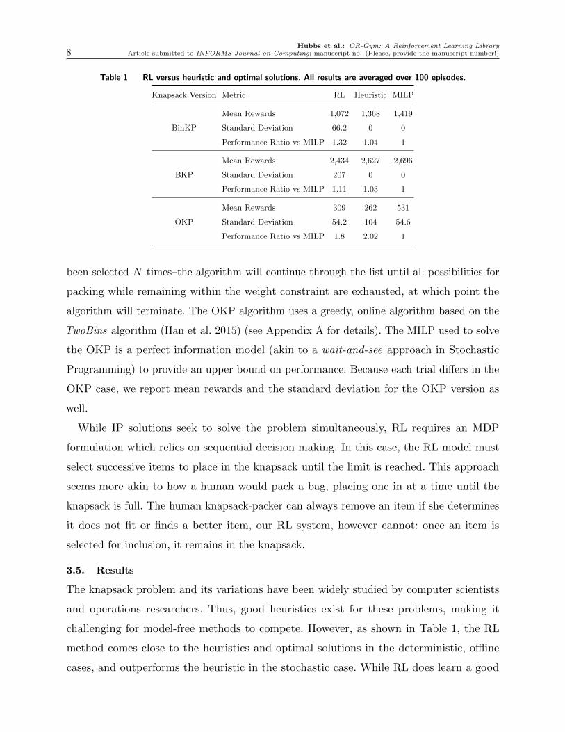
reorder quantity is given by Equation 6, where zm is the base-stock level at stage m and

the term in the summation is the current inventory position at the beginning of period t.

Rmt = max

(0, zm−

m∑m′=1

(Im

′

t +Tm′

t −Bm′

t−1

))∀m∈M, t∈ T (6)

Glasserman and Tayur (1995) propose a method called infinitesimal perturbation analysis

(IPA) to determine the optimal base-stock level. IPA is a gradient descent approach that

minimizes the expected cost over a sample path. IPA relies on perturbing a simulated

sample path iteratively until the desired improvement in the objective function is obtained.

Derivatives are calculated or estimated explicitly to provide the updates necessary for the

gradient descent. To guarantee convergence, the optimization is performed offline. In the

IPA implementation for the base-stock policy, a simulated sample path of T periods is

run with fixed base-stock levels. The gradients for the state variables (inventory positions,

reorder quantities, etc) are determined from the recursive relations in the model defined in

Appendix D. These are used to update the base stock levels. The updated levels are applied

to the same simulated sample path over T periods (iteration number 2). The process is

repeated until the base stock levels stabilize or the change in the objective function is below

a certain tolerance.

In the present work, we follow this idea of optimizing over a sample path, but apply

more robust approaches for the optimization. We use the objective function given below.

f =1

|T |ED

[∑m∈M

Pmt

](7)

Since the objective function for the IMP (normalized expected profit over the sample path,

Equation 7) is non-smooth and non-differentiable for discrete demand distributions, line

search algorithms based on the Wolfe conditions (Nocedal and Wright 2006) often fail to

converge when determining the step size for the classical IPA approach. Instead of settling

on taking full step sizes or using an ad hoc approach when determining the step sizes,

derivative-free optimization (DFO) based on Powell’s method (Powell 1964) can be used.

Another approach available for IMP is that of mixed-integer programming (MIP), which

readily expresses the discontinuities in the model equations using binary variables and can

guarantee finding the optimal base stock levels over a sample path.

The benefit of using Powell’s method (Powell 1964) is that it does not rely on gradients

and can be applied to non-differentiable systems. Since the demand distributions are


Table 3 Parameters values for both Inventory Management Environments

Parameter Symbol Stage 0 Stage 1 Stage 2 Stage 3

Initial Inventory I0 100 100 200 -

Unit Sales Price p $2.00 $1.50 $1.00 $0.75

Unit Replenishment Cost r $1.50 $1.00 $0.75 $0.50

Unit Backlog Cost k $0.10 $0.075 $0.05 $0.025

Unit Holding Cost h $0.15 $0.10 $0.05 -

Production Capacity c - 100 90 80

Lead Times L 3 5 10 -

discrete, Powell’s method is followed by either rounding the base stock levels to the nearest

integer or performing a local search to find the nearest optimal integer solution. In the

latter case, enumeration is used to compare all neighboring integer solutions to the solution

found by Powell’s method.

In the MIP approach, the disjunctions arising from the minimum and maximum operators

in the model are reformulated into algebraic inequalities using Big-M reformulations.

A third approach to the IMP is to use a dynamic reorder policy that is determined by

solving a linear program (LP) at each time period with a shrinking horizon (SHLP). This

approach requires prior knowledge of the demand probability distribution and assumes the

expected value of the demand for all time periods in the optimization horizon. After solving

the optimization for the current time period in the simulation, the optimal reorder action

found for the current period is implemented. All future reorder actions are discarded and

the process is repeated in each subsequent time period as the simulation marches forward.

5.3. Results

Two examples are run to compare the OR (DFO, MIP, and SHLP) and RL approaches in

the IMP (simulation parameters are provided in Table 3). It should be noted that the DFO

and MIP approaches use static base stock policies, whereas the SHLP and RL approaches

use dynamic reorder policies. Both approaches are compared to a perfect information LP

model (PILP), which is an LP model that determines the optimal dynamic reorder policy

for that run by using the actual demand values for each time period. InvManagement-v0 is a

30-period, 4 stage supply chain with backlog. A Poisson distribution is used for the demand

with a mean of 20. A discount factor for the time value of money of 97% percent is used

(3% discount). The second problem, InvManagement-v1, is identical to InvManagement-v0,

except it operates under lost sales rather than an order backlog.


Figure 6 Training curves smoothed over 100 episodes for RL algorithm compared to the PILP, SHLP, and MILP

base-stock models. Shaded areas indicate standard deviation of rewards.

Training curves for both environments, v0 and v1, as well as the mean values for the

PILP, SHLP, and MILP models are given in Figure 6.

For the InvManagement-v0 environment, the RL model outperformed the static policy

models, but was outperformed by the shrinking horizon model, achieving a performance

ratio of 1.2 (Table 4). The daily rewards for each of the compared models are given in

Figure 7, where it can be seen that the RL model’s rewards track closely with the PILP

and SHLP models before leveling off towards the end of the episode. The model does this

because it has been trained on a 30-day episode, and, unlike the static base stock policy

models, it does not need to continue to order additional inventory towards the end of the

run because the holding costs become large and the extra stock will not be sold within the

episode. This behavior is shown in the inventory plots given in Figure 8, where the RL

inventory levels decrease as the episode progresses, as is also observed with the PILP and

SHLP models, which are also aware of the limited horizon.

The static policy models do not exhibit this behavior and continue targeting the optimal

base stock levels, which increases the holding costs and causes the profit to suffer. However,

in a real application, the supply chain is likely to operate for more than 30 days, and

dropping inventories towards the end of the run would be detrimental to the supply chain’s

performance beyond the 30 days. In this case, the RL model could be trained on a continuous

environment with monthly cycles.

The RL model in InvManagement-v1 (no backlog orders), performs slightly worse relative

to the PILP with a performance ratio of 1.3 (Table 4). The same end-of-episode dynamics

observed in InvManagement-v0 are also visible in Figure 9.

For both environment variations, the RL model outperforms the static policy models,

scoring performance ratios between 1.2-1.3. This shows the potential for RL to learn

competitive, dynamic policies for multi-stage inventory management problems.


Table 4 Total reward comparison for InvManagement problems and the various models used to solve them.

InvManagement-v0 RL SHLP DFO MIP PILP

Mean Rewards 438.8 508.0 360.9 388.0 546.8

Standard Deviation 30.6 28.1 39.9 30.8 30.3

Performance Ratio vs PILP 1.2 1.1 1.5 1.4 1.0

InvManagement-v1 RL SHLP DFO MIP PILP

Mean Rewards 409.8 485.4 364.3 378.5 542.7

Standard Deviation 17.9 29.1 33.8 26.1 29.9

Performance Ratio vs PILP 1.3 1.1 1.5 1.4 1.0

Figure 7 Cumulative profit for both inventory management models. Results averaged over 10 episodes. Shaded

areas indicate standard deviation of rewards.

Figure 8 Average inventory on hand at each echelon for InvManagement-v0.


Figure 9 Average inventory on hand at each echelon for InvManagment-v1.

6. Asset Allocation

Asset allocation refers to the task of creating a collection (portfolio) of financial assets as

to maximize an investors return, subject to some investment criteria and constraints. The

most famous approach to portfolio optimization stems from Markowitz’s mean-variance

framework from the 1950s that frames portfolio optimization as a trade-off between the

return of an asset (modeled using its expected value) and the risk associated with the

asset (modeled by its variance) (Markowitz 1952). Since then, the asset allocation problem

has been extensively explored in the literature with a multitude of models that take into

account many different practical considerations (see Black and Litterman (1992), Perold

(1984), Fabozzi et al. (2007), Konno and Yamazaki (1991), Krokhmal et al. (2003), and

DeMiguel et al. (2009)).


Here, we focus on the multi-period asset allocation problem (MPAA) of Dantzig and Infanger

(1993). An investor starts with a portfolio x0 = [x01, ..., x

0n] consisting of n assets, with an

additional quantity of cash we call a “zero” asset, x00. The investor wants to determine the

optimal distribution of assets over the next L periods to maximize total wealth at the end

of the final investment horizon of total length L.

The optimization variables are bli (the amount of asset i bought at the beginning of

period l) and sli (the amount sold) where i= 1, ..., n and l= 1, ...,L.

The price of an asset i in period l is denoted by P li . We assume that the cash account is

interest-free meaning that P l0 = 1,∀l. The sales and purchases of an asset i in period l are


given by proportional transaction costs αli and βl

i, respectively. These prices and costs are

subject to change asset-to-asset and period-to-period.

The deterministic version of this problem is given by the following formulation:

maxx,s,b

n∑i=0

PLi x

Li (8a)

xl0 ≤ xl−10 +

n∑i=1

(1−αli)P

li s

li−

n∑i=1

(1 +βli)P

li b

li ∀l ∈L (8b)

xli = xl−1i − sli + bli ∀i∈ n ∀l ∈L (8c)

sli, bli, x

li ≥ 0 ∀i∈ n ∀l ∈L (8d)

This is a linear programming problem that can be easily solved by common optimization

solvers.

In the RL environment, we consider the optimization of a portfolio derived from Equations

8. This portfolio initially contains $100 in cash and three other assets and our goal is to

optimize portfolio value over a time horizon of 10 periods. Of course, the prices of each

asset for each period are not known in advance. Consequently, these prices are modeled as

Gaussian random variables with a fixed mean and variance for each asset in each period. In

each instantiation of the environment, these prices take on a new value. Transaction costs

are fixed in all instances.

Each step in the RL environment corresponds to a single investment period. The state of

the environment, s, at a particular period is described by the following vector of the current

period, l, as well as cash and asset quantities and prices, corresponding to the notation of

(Equations 8):

s=[l, xl0, x

l1, x

l2, x

l3, P

l1, P

l2, P

l3

](9)

At each step, the RL agent must decide how much, if any, of each particular asset to buy

or sell. The action, a, is described by the following vector of amounts of the three assets to

buy or sell, corresponding to the notation of from Equations 8:

a=[δl1, δ

l2, δ

l3

](10)

where,

δli =

sli (bli = 0), for δli < 0

bli (bli = 0), for δli > 0

sli, bli = 0 for δli = 0


δli ∈[− 2000,2000

]The reward r is given only at the very end of the episode and is equal to the value of the

objective function of Equation 8a (i.e. the portfolio value). An alternative design choice

that we considered was to give a reward at each step (for example, the current portfolio

value). This implementation did prove to facilitate learning but we chose the sparse-reward

formulation to demonstrate the power of RL even in relatively challenging situations.

6.2. OR Methods

Robust optimization (RO) is an established field in operations-research that rigorously

addresses decision-making under uncertainty. In the robust optimization paradigm, opti-

mization problem parameters are treated as unknown quantities bounded by an uncertainty

set. It is the objective of RO to find good solutions that are feasible no matter what values

within the uncertainty set the problem parameters take (Ben-Tal et al. 2009). In essence,

robust optimization allows the practitioner to optimize the worst-case scenario.

To benchmark the performance of the RL agent, we formulate and solve the corresponding

robust-optimization problem as given in Equations 8, originally from Ben-Tal et al. (2000).

Constraints on cash flow are modeled using a 3−σ approach such that the chosen investment

policy will be feasible in 99.7% of possible scenarios. The goal of the optimization is to

find an investment policy such that the portfolio value will be greater than or equal to the

objective function value of the optimization problem. We refer the reader to Cornuejols

and Tutuncu (2006) for a clear description and explanation of the robust formulation.

We then take the investment policy (i.e. the amount of each asset to buy and sell in each

period) and simulate this policy for several different realizations of the parameters within

the uncertainty set. We use the average rewards achieved as a benchmark against the policy

found by the RL agent.

An alternative to the robust optimization approach would have been to use multi-stage

stochastic programming (MSP). To paraphrase the arguments of Ben-Tal et al. (2000), RO

was highlighted instead because: it is much more tractable than the MSP, any simplifying

implementation of MSP (e.g. by solving on a rolling-horizon) would be ad hoc and would not

necessarily yield a superior solution than the RO approach, and, although the RO approach

seems ‘conservative’, the mathematical form of the RO is such that the RO solution is


not as conservative as it may seem. As important, a central goal of asset allocation is not

only to maximize expected rewards, but also to minimize risk. Robust optimization, which

minimizes the downside-risk, is a natural approach to achieve portfolios with high returns

under a variety of market conditions. As the results of Ben-Tal et al. (2000) show for this

problem, not only does RO match the performance of MSP in terms of mean portfolio

value, the standard-deviation (and hence the risk) of the return is substantially lower.

We solve the RO model using BARON 19.7.13 on a 2.9 GHz Intel i7-7820HQ CPU

(Sahinidis 1996).

6.3. Results

The solution to the deterministic optimization problem, where all prices (equal to their

mean values in the RO and RL formulations) are known with certainty, is $17,956.20.

However, this value is not practically important because market prices are never known in

advance.

The robust optimization solution is a more practically important metric for comparison.

While the uncertainty set chosen is conservative, the RO approach multiplies the initial

$100 in cash to a portfolio value of at least $610.17 for 99.7% of the parameter space. This

value corresponds to the objective function value of the RO problem, and is the worst-case

return.

The solution to the RO problem corresponds to an investment strategy. When we take

the RO strategy and actually apply it in 103 randomly generated instances of this problem,

we see that the RO policy is able to multiply the initial cash to an average portfolio value of

about $865 with a standard deviation of roughly $80. Results for the RL and RO approaches

are given in Figure 10.

We see that, despite the sparse-reward formulation, the RL agent is able to successfully

learn a policy that, on average, yields higher portfolio values than the strategy given by

RO. Purely in the sense of maximizing expected portfolio value, RL is a strong alternative

to robust optimization. On the downside however, the variance of the RL portfolio values is

higher than in the case of RO. Consequently, RO seems to be the better alternative when

our primary concern is risk, achieving worst-case returns that are much higher than those

from RL. As a final note, the number of episodes required to train the RL agent was very

high, resulting in a training time on the order of hours. On the other hand, the robust

optimization policy was found in just a few minutes.


Figure 10 Training rewards for RL algorithm smoothed over 100 episodes and average rewards given by imple-

menting robust optimization solution. Shaded areas indicate standard deviation of rewards. Histogram

compares results from 1,000 simulated episodes for RL and RO. Notice the wider distribution and

skew of the RL solution which offers less downside protection.

7. Conclusion

We have developed a library of reinforcement learning environments consisting of classic

operations research problems. RL traditionally relies on environments being formulated

as Markov Decision Processes (MPDs). These are sequential decision processes where a

decision or action in one state influences the transition to the subsequent state. In many

optimization problems, sequential decisions are required making RL straightforward to

apply to the problem. Hard constraints can be imposed on RL agents via action masking,

whereby the probability associated with selecting an action that would lead to a constraint

violation are set to 0 ensuring these actions are not selected. The use of action masking

reduces the search space and can both improve the learned policy and reduce the amount

of training time required by the model.

Additionally, we have provided benchmarks for four problem classes showing results

for RL, heuristics, and optimization models. In all cases, RL is capable of learning a

competent policy. RL outperforms the benchmark in many of the more complex and

difficult environments where uncertainty plays a significant role, and may be able to provide

value in similar, industrial applications. RL did not outperform the heuristic models in

the off-line knapsack problems. This does not come as a complete surprise given that

the knapsack problem has been well-studied for many decades, and numerous heuristics

have been developed to solve the problem and increase the state-of-the-art solutions. In

cases such as this, the additional complexity and computational costs of RL may not be

worthwhile.

RL provides a general framework to solve these various problems. Each system was solved

with the same algorithm using three layers and 128 nodes each and minor hyperparameter


tuning for the learning rate and entropy loss within a standard library. With new tools

such as Ray, RL becomes increasingly accessible for solving classic optimization problems

under uncertainty as well as industrial equivalents where optimization models do not exist,

or are too expensive to develop and compute online.

It may be possible to extract rules from the RL policies to develop better heuristic

solutions for each of the problems. Additionally, given the structure of these problems and

the fact that optimization models exist for them, the area is rife for exploration of hybrid

RL and mathematical programming approaches which can combine the speed and flexibility

of RL with the solutions available from mathematical programming to improve results and

time to solution. Another interesting avenue to pursue is the use of graph neural networks

and RL, which may be able to benefit from the structure of these models. Finally, the

OR-Gym library contains additional environments from the literature for experimentation.1

References

Baker BS, Schwarz JS (1983) Shelf Algorithms for Two-Dimensional Packing Problems. SIAM Journal of

Computing 12(3):508–526.

Balaji B, Bell-Masterson J, Bilgin E, Damianou A, Garcia PM, Jain A, Luo R, Maggiar A, Narayanaswamy

B, Ye C (2019) ORL: Reinforcement Learning Benchmarks for Online Stochastic Optimization Problems

URL http://arxiv.org/abs/1911.10641.

Bansal N, Oosterwijk T, Vredeveld T, van der Zwaan R (2016) Approximating Vector Scheduling: Almost

Matching Upper and Lower Bounds. Algorithmica 76(4):1077–1096.

Bellman R (1957) A Markovian decision process. Journal Of Mathematics And Mechanics 6:679–684.

Ben-Tal A, El Ghaoui L, Nemirovsky A (2009) Robust Optimization (Princeton University Press).

Ben-Tal A, Margalit T, Nemirovski A (2000) Robust modeling of multi-stage portfolio problems. High

Performance Optimization, 303–323.

Berner C, Brockman G, Chan B, Cheung V, Dennison C, Farhi D, Fischer Q, Hashme S, Hesse C, Jozefowicz

R, Gray S, Olsson C, Pachocki J, Petrov M, Ponde de Oliveira Pinto H, Raiman J, Salimans T, Schlatter

J, Schneider J, Sidor S, Sutskever I, Tang J, Wolski F, Zhang S (2019) Dota 2 with Large Scale Deep

Reinforcement Learning. Technical report, URL https://arxiv.org/abs/1912.06680.

Bertsimas D, Thiele A (2006) A robust optimization approach to inventory theory. Operations Research

54(1):150–168.

Black F, Litterman R (1992) Global portfolio optimization. Financial Analysts Journal 48(5).

1 The full list of envirionments, as well as download and installation instructions can be found here: https://github.com/hubbs5/or-gym

http://arxiv.org/abs/1911.10641

https://arxiv.org/abs/1912.06680




Brockman G, Cheung V, Pettersson L, Schneider J, Schulman J, Tang J, Zaremba W (2016) OpenAI Gym

1–4.

Christensen HI, Khan A, Pokutta S, Tetali P (2017) Approximation and online algorithms for multidimensional

bin packing: A survey. Computer Science Review 24:63–79.

Chu Y, You F, Wassick JM, Agarwal A (2015) Simulation-based optimization framework for multi-echelon

inventory systems under uncertainty. Computers and Chemical Engineering 73:1–16.

Coffman EG, Csirik J, Galambos G, Martello S, Vigo D (2013) Bin Packing Approximation Algorithms:

Survey and Classification. Handbook of Combinatorial Optimization, 455–531 (Heidelberg: Springer).

Cornuejols G, Tutuncu R (2006) Chapter 20: Robust Optimization Models in Finance. Optimization Methods

in Finance, 309–312.

Cortez E, Bonde A, Muzio A, Russinovich M, Fontoura M, Bianchini R (2017) Resource Central: Understanding

and Predicting Workloads for Improved Resource Management in Large Cloud Platforms. Proceedings

of the International Symposium on Operating Systems Principles (SOSP).

Courcoubetis C, Weber R (1990) Stability of on-line bin packing with random arrivals and long-run-average

constraints. Probability in the Engineering and Informational Sciences 4(4):447–460.

Csirik J, Johnson DS, Kenyon C, Orlin JB, Shor PW, Weber RR (2006) On the Sum-of-Squares algorithm

for bin packing. Journal of the ACM 53(1):1–65.

Dantzig GB (1957) Discrete-Variable Extremum Problems. INFORMS 5(2):266–277.

Dantzig GB, Infanger G (1993) Multi-stage stochastic linear programs for portfolio optimization. Annals of

Operations Research 45:59–76.

DeMiguel V, Garlappi L, Nogales FJ, Uppal R (2009) A Generalized Approach to Portfolio Optimization:

Improving Performance by Constraining Portfolio Norms. Management Science 55(9).

Eruguz AS, Sahin E, Jemai Z, Dallery Y (2016) A comprehensive survey of guaranteed-service models for

multi-echelon inventory optimization.

Fabozzi FJ, Kolm PN, Pachamanova DA, Focardi SM (2007) Robust Portfolio Optimization and Management

(John Wiley & Sons).

Gilmore PC, Gomory RE (1961) A Linear Programming Approach to the Cutting-Stock Problem. Operations

Research 9(6):849–859.

Glasserman P, Tayur S (1995) Sensitivity analysis for base-stock levels in multiechelon production-inventory

systems. Management Science 41(2):263–281.

Gupta V, Radovanovic A (2012) Online Stochastic Bin Packing 1–21, URL http://arxiv.org/abs/1211.

2687.

Gurobi Optimization LLC (2018) Gurobi. URL https://www.gurobi.com.



https://www.gurobi.com


Han X, Kawase Y, Makino K (2015) Randomized algorithms for online knapsack problems. Theoretical

Computer Science 562(C):395–405.

Hart WE, Laird CD, Woodruff DL, Hackebeil GA, Nicholson BL, Siirola JD (2017) Pyomo — Optimization

Modeling in Python (Cham, Switzerland: Springer), 2nd edition.

Hubbs CD, Li C, Sahinidis NV, Grossmann IE, Wassick JM (2020) A deep reinforcement learning approach

for chemical production scheduling. Computers and Chemical Engineering .

Johnson DS (1974) Approximation algorithms for combinatorial problems. Journal of Computer and System

Sciences 9(3):256–278.

Kapuscinski R, Tayur S (1999) Optimal policies and simulation-based optimization for capacitated production

inventory systems. Quantitative Models for Supply Chain Management, 7–40 (Springer).

Kellerer H, Pferschy U, Pisinger D (2004) Knapsack Problems, volume 53 (Heidelberg: Springer Verlag).

Kong W, Sivakumar D, Liaw C, Mehta A (2019) A new dog learns old tricks: RL finds Classic optimization

algorithms. 7th International Conference on Learning Representations, ICLR 2019 (2009):1–25.

Konno H, Yamazaki H (1991) Mean-Absolute Deviation Portfolio Optimization Model and Its Applications

to Tokyo Stock Market. Management Science 37(5).

Kool W, Van Hoof H, Welling M (2019) Attention, learn to solve routing problems! 7th International

Conference on Learning Representations, ICLR 2019 1–25.

Krokhmal P, Palmquist J, Uryasev S (2003) Portfolio optimization with conditional value-at-risk objective

and constraints. Journal of Risk 4(2).

Lee HL, Padmanabhan V, Whang S (1997) Information distortion in a supply chain: The bullwhip effect.

Management Science 43(4):546–558.

Li Y (2017) Deep Reinforcement Learning: An Overview 1–70.

Lueker GS (1995) Average-case analysis of off-line and on-line knapsack problems. Proceedings of the Annual

ACM-SIAM Symposium on Discrete Algorithms (January 1995):179–188.

Ma W, Simchi-Levi D, Zhao J (2019) A Competitive Analysis of Online Knapsack Problems with Unit

Density. SSRN Electronic Journal .

Marchetti-Spaccamela A, Vercellis C (1995) Stochastic on-line knapsack problems. Mathematical Programming

68(1-3):73–104.

Markowitz H (1952) Portfolio Selection. The Journal of Finance 7(1):77–91.

Martinez Y, Nowe A, Suarez J, Bello R (2011) A Reinforcement Learning Approach for the Flexible Job Shop

Scheduling Problem. Coello CA, ed., Learning and Intelligent Optimization, 253–262 (Springer Verlag).

Mathews GB (1896) On the Partition of Numbers. Proceedings of the London Mathematical Society s1-

28(1):486–490.


Moritz P, Nishihara R, Wang S, Tumanov A, Liaw R, Liang E, Elibol M, Yang Z, Paul W, Jordan MI, Stoica

I (2018) Ray: A Distributed Framework for Emerging AI Applications URL http://arxiv.org/abs/

1712.05889.

Mortazavi A, Arshadi Khamseh A, Azimi P (2015) Designing of an intelligent self-adaptive model for supply

chain ordering management system. Engineering Applications of Artificial Intelligence 37:207–220.

Nocedal J, Wright S (2006) Numerical optimization (Springer Science & Business Media).

Oroojlooyjadid A, Nazari M, Snyder L, Takac M (2017) A Deep Q-Network for the Beer Game: A Reinforcement

Learning algorithm to Solve Inventory Optimization Problems 1–38, URL http://arxiv.org/abs/

1708.05924.

Perold AF (1984) Large-scale portfolio optimization. Management Science 30(10).

Powell MJD (1964) An efficient method for finding the minimum of a function of several variables without

calculating derivatives. The Computer Journal 7(2):155–162.

Ram B (1992) The pallet loading problem: A survey. International Journal of Production Economics

28(2):217–225.

Sahinidis NV (1996) BARON: A general purpose global optimization software package. Journal of Global

Optimization 8(2):201–2015.

Schulman J, Moritz P, Levine S, Jordan MI, Abbeel P (2016) High-dimensional continuous control using

generalized advantage estimation 1–14, URL https://arxiv.org/pdf/1506.02438.pdf.

Silver D, Hubert T, Schrittwieser J, Antonoglou I, Lai M, Guez A, Lanctot M, Sifre L, Kumaran D, Graepel

T, Lillicrap T, Simonyan K, Hassabis D (2017) Mastering Chess and Shogi by Self-Play with a General

Reinforcement Learning Algorithm 1–19, URL http://arxiv.org/abs/1712.01815.

Simchi-Levi D, Zhao Y (2012) Performance Evaluation of Stochastic Multi-Echelon Inventory Systems: A

Survey. Advances in Operations Research 2012:126254.

Song W, Xiao Z, Chen Q, Luo H (2014) Adaptive resource provisioning for the cloud using online bin packing.

IEEE Transactions on Computers 63(11):2647–2660.

Sutton R, Barto A (2018) Reinforcement Learning: An Introduction (Cambridge, Massachusetts: MIT Press),

2 edition.





https://arxiv.org/pdf/1506.02438.pdf


Documents

OR-Gym: A Reinforcement Learning Library for Operations