Embed Size (px)
Citation preview
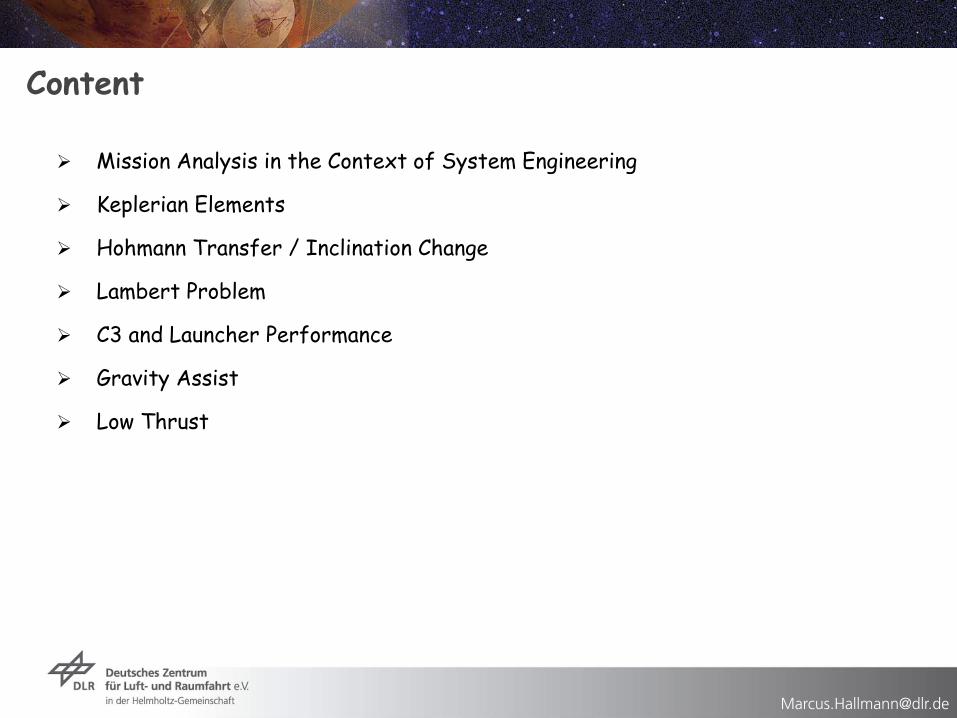
Content
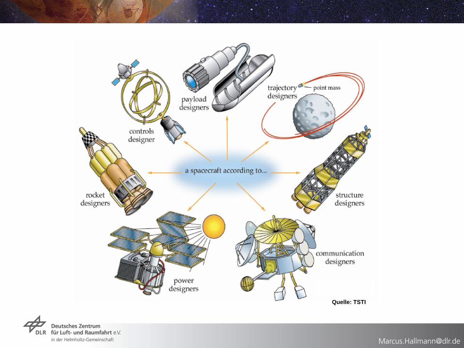
Mission Analysis in the Context of System Engineering
Keplerian Elements
Hohmann Transfer / Inclination Change
Lambert Problem
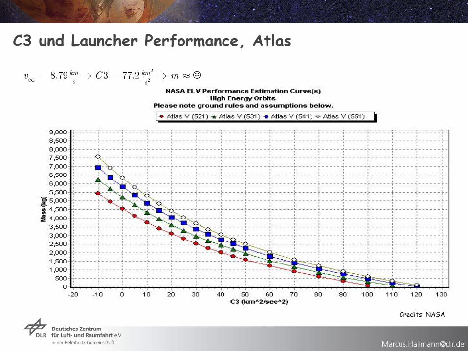
C3 and Launcher Performance
Gravity Assist
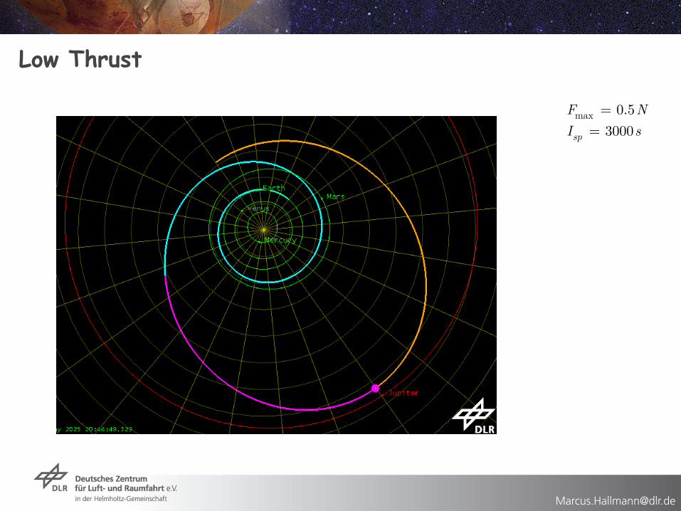
Low Thrust
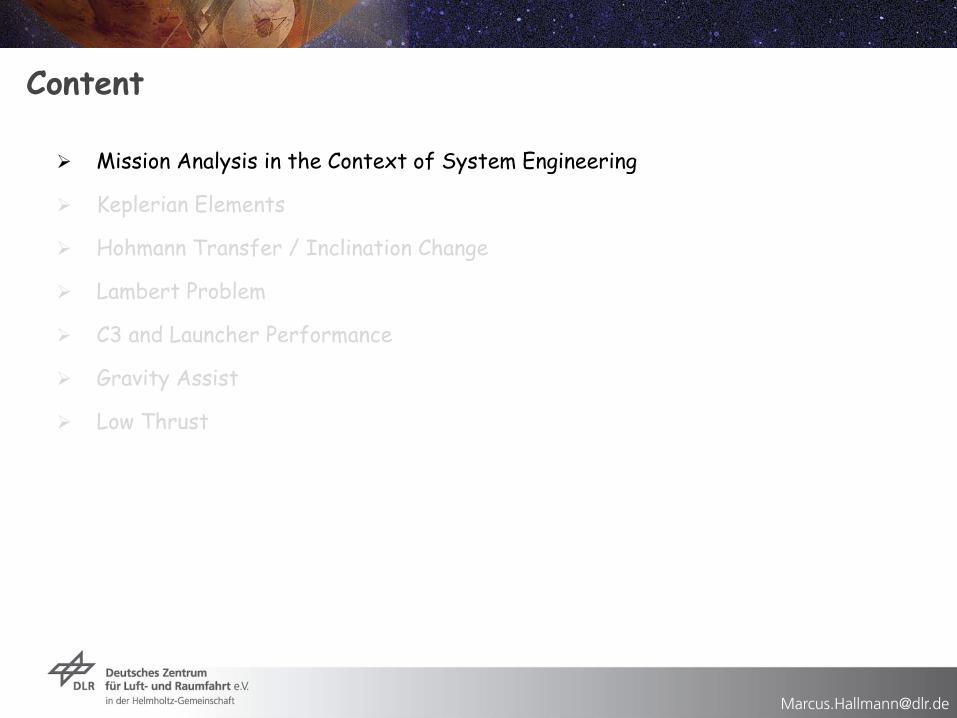
Content
Mission Analysis in the Context of System Engineering
Keplerian Elements
Hohmann Transfer / Inclination Change
Lambert Problem
C3 and Launcher Performance
Gravity Assist
Low Thrust
The Orbit Design Process
Establish orbit types
Determine orbit related requirements
Assess launch options
Create ΔV budget
Perform orbit design trades
Determine orbit related requirements
Temperature gradient
Absolute temperature
Straylight reduction
Max eclipse time
Communication requirements ( volume, timeliness )
Sun-Spacecraft-Earth angle
Scan strategy
Attitude disturbance reduction
Radiation (total dose over mission time)
…

Content
Mission Analysis in the Context of System Engineering
Keplerian Elements
Hohmann Transfer / Inclination Change
Lambert Problem
C3 and Launcher Performance
Gravity Assist
Low Thrust
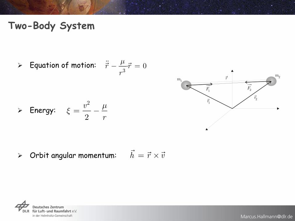
Equation of motion:
Energy:
Orbit angular momentum:
Two-Body System
3· 0r r
r
m- =
2
2
v
r
mx = -
h r v= ´
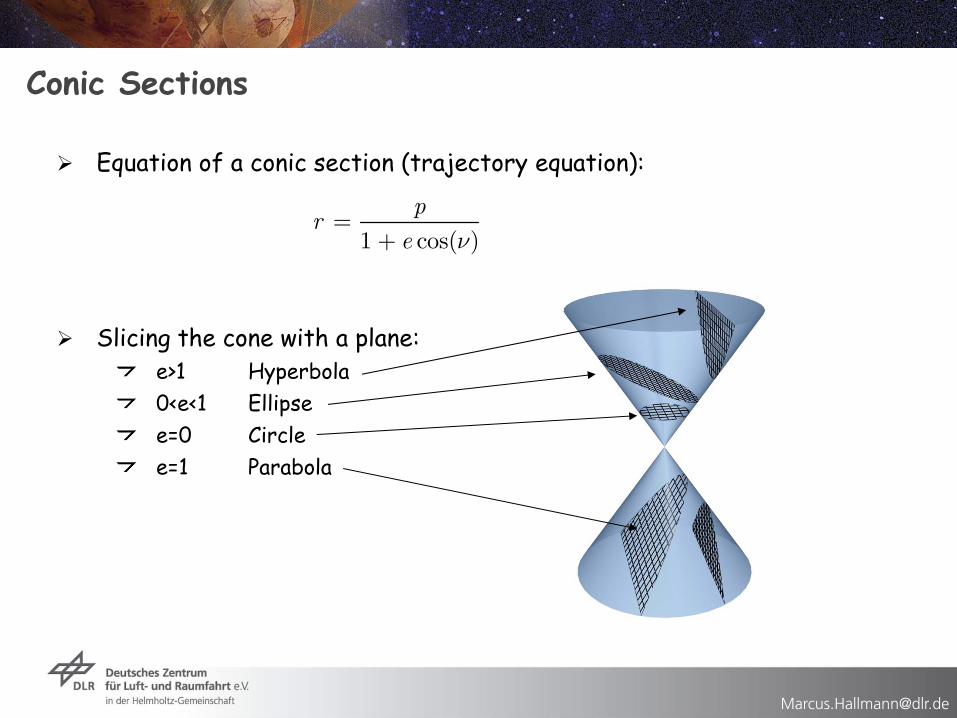
Conic Sections
Equation of a conic section (trajectory equation):
Slicing the cone with a plane:e>1 Hyperbola0<e<1 Ellipsee=0 Circlee=1 Parabola
1 cos( )
pr
e n=
+
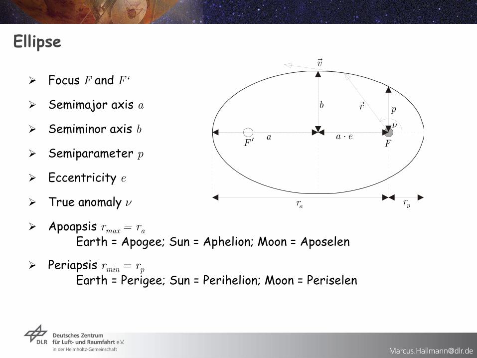
Ellipse
Focus F and F‘
Semimajor axis a
Semiminor axis b
Semiparameter p
Eccentricity e
True anomaly n
Apoapsis rmax = ra
Earth = Apogee; Sun = Aphelion; Moon = Aposelen
Periapsis rmin = rp
Earth = Perigee; Sun = Perihelion; Moon = Periselen
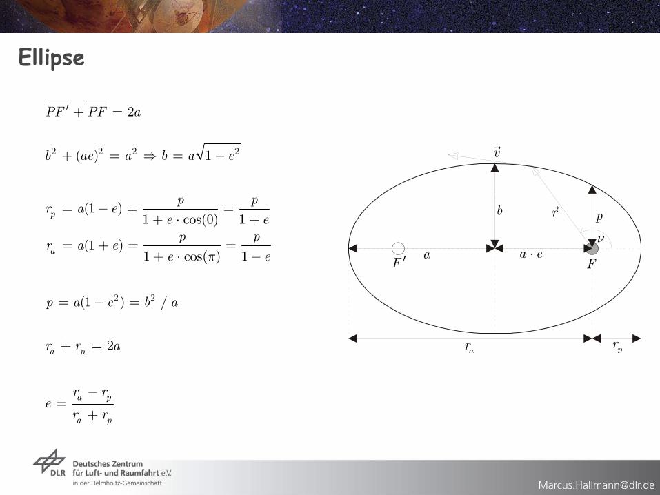
Ellipse
2PF PF a¢ + =
2 2 2 2( ) 1b ae a b a e+ = = -
(1 )1 cos(0) 1
(1 )1 cos( ) 1
p
a
p pr a e
e ep p
r a ee ep
= - = =+ ⋅ +
+ = ==+ ⋅ -
2 2(1 ) /p a e b a= - =
2a pr r a+ =
a p
a p
r re
r r
-=
+
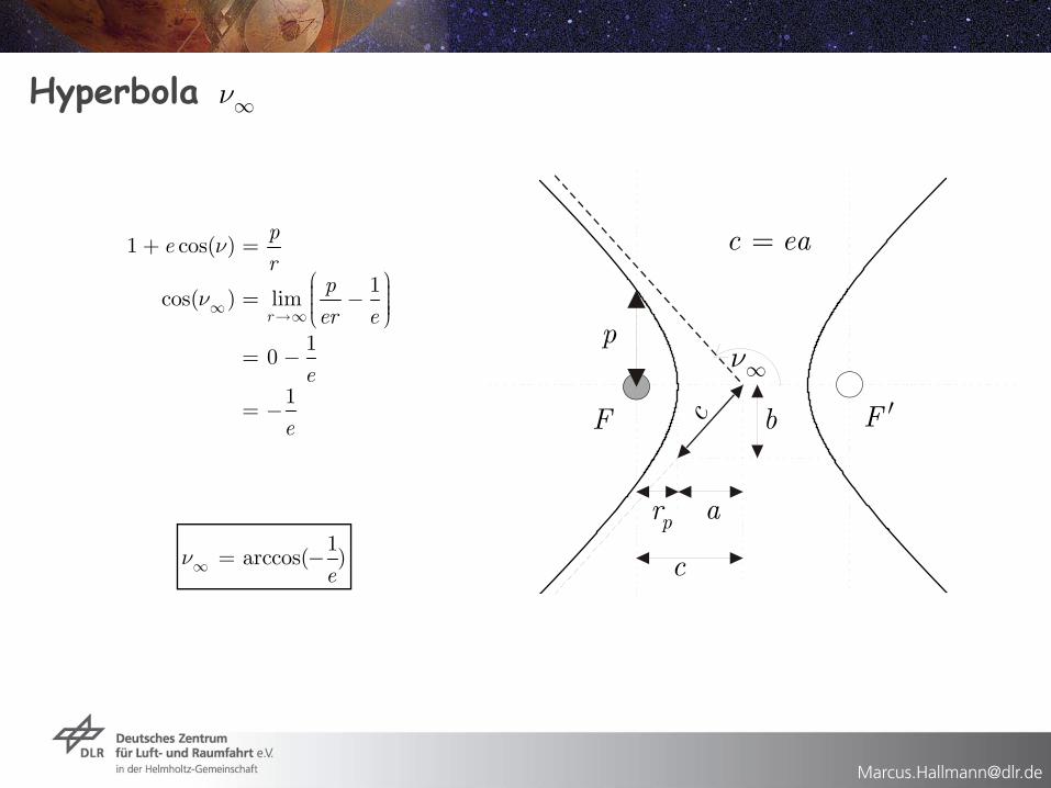
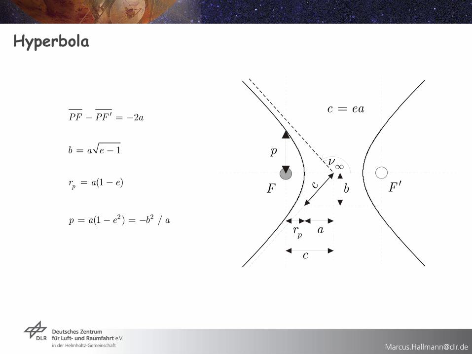
Hyperbola
1 cos( )
1cos( ) lim
10
1
r
pe
rp
er e
e
e
n
n¥ ¥
+ =
æ ö÷ç= - ÷ç ÷ç ÷è ø
= -
= -
n¥
1arccos( )
en¥ = -
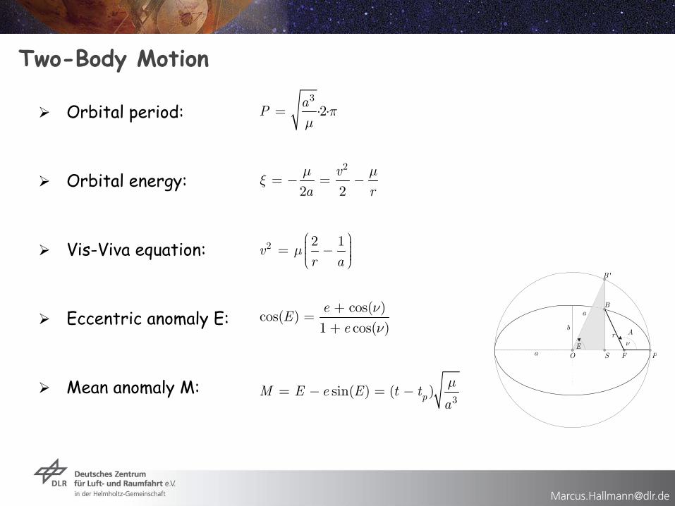
Two-Body Motion
Orbital period:
Orbital energy:
Vis-Viva equation:
Eccentric anomaly E:
Mean anomaly M:
3
·2·a
P pm
=
2 2 1v
r amæ ö÷ç= - ÷ç ÷ç ÷è ø
2
2 2
v
a r
m mx = - = -
3sin( ) ( )pM E e E t t
a
m= - = -
cos( )cos( )
1 cos( )
eE
e
nn
+=
+
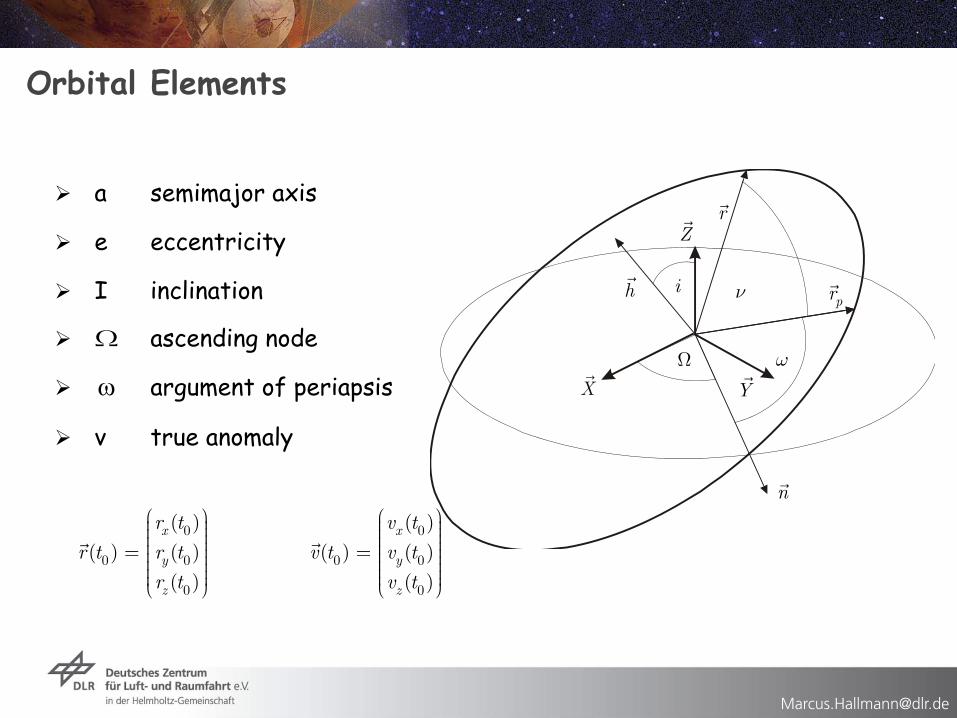
Orbital Elements
a semimajor axis
e eccentricity
I inclination
Ω ascending node
ω argument of periapsis
ν true anomaly
0 0
0 0 0 0
0 0
( ) ( )
( ) ( ) ( ) ( )
( ) ( )
x x
y y
z z
r t v t
r t r t v t v t
r t v t
æ ö æ ö÷ ÷ç ç÷ ÷ç ç÷ ÷ç ç÷ ÷ç ç= =÷ ÷ç ç÷ ÷ç ç÷ ÷÷ ÷ç ç÷ ÷ç çè ø è ø
Content
Mission Analysis in the Context of System Engineering
Keplerian Elements
Hohmann Transfer / Inclination Change
Lambert Problem
C3 and Launcher Performance
Gravity Assist
Low Thrust
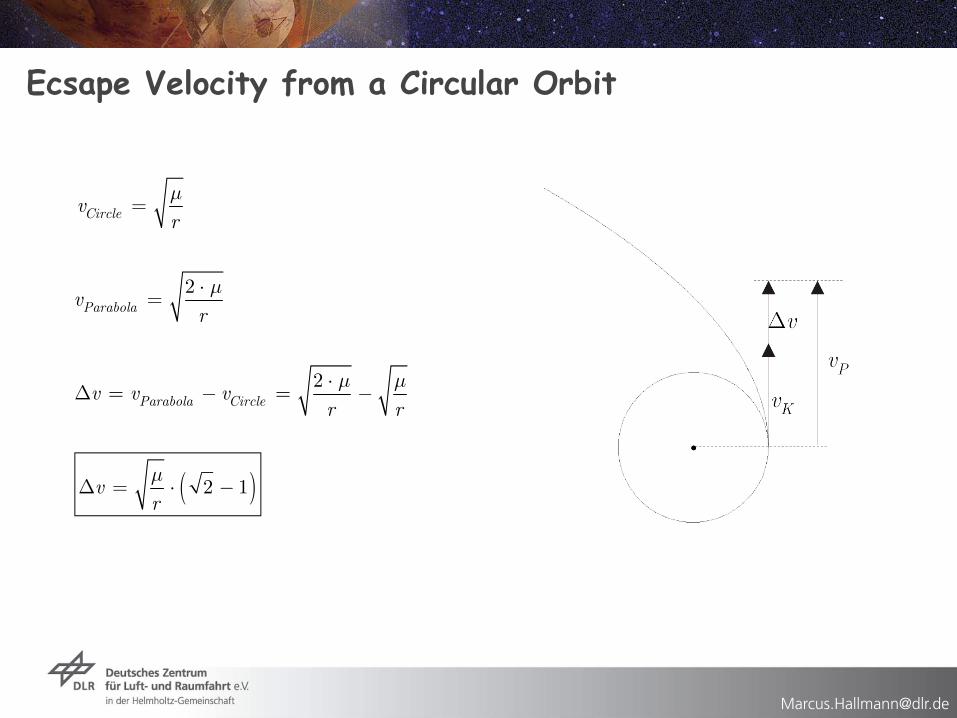
Ecsape Velocity from a Circular Orbit
Circlevr
m=
2Parabolav
r
m⋅=
2CiParabol ca r lev v v
r r
m m⋅D = = --
( )2 1D = ⋅ -vr
m
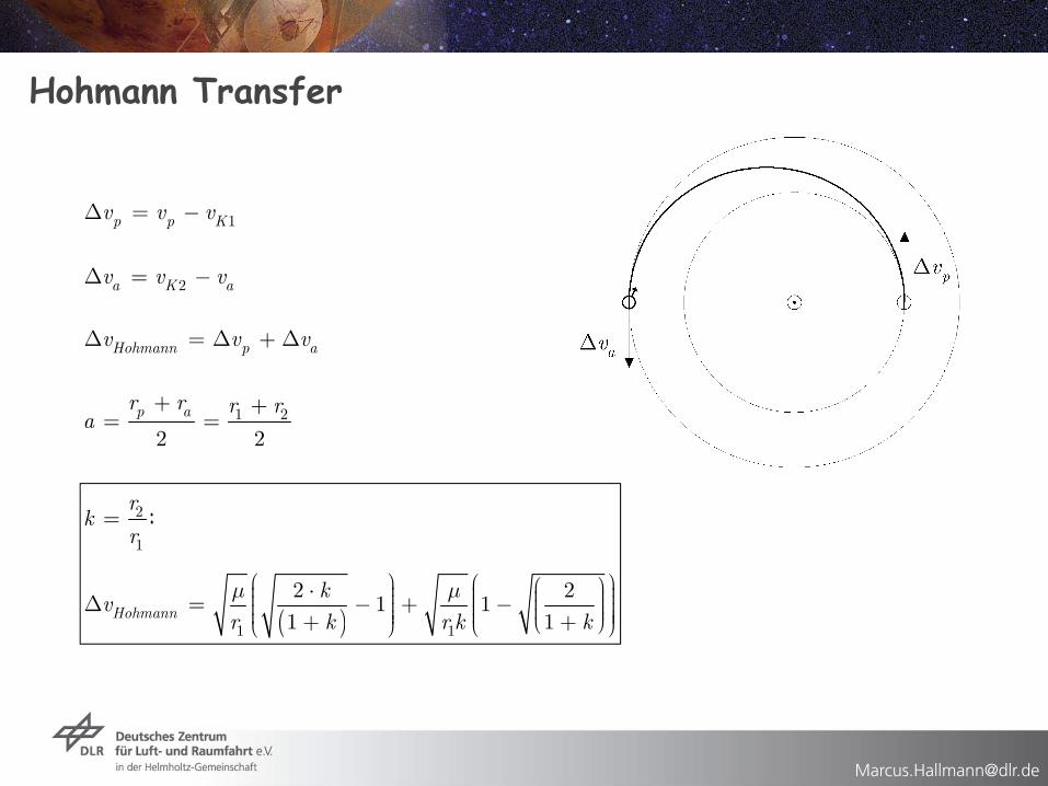
Hohmann Transfer
1D = -p p Kv v v
2D = -a K av v v
D = D + DHohmann p av v v
1 2
2 2
+ += =p ar r r r
a
( )1 1
2
1
21 1
1 1
2Hohmann
kv
r k r
k
k
r
r
k
m mæ ö æ öæ ö⋅ ÷ ÷ç ç ÷ç÷ ÷ç çD = - + - ÷ç÷ ÷ç ÷ç ç÷ ÷÷÷÷ çç è ø+ +è øè
=
ø
:
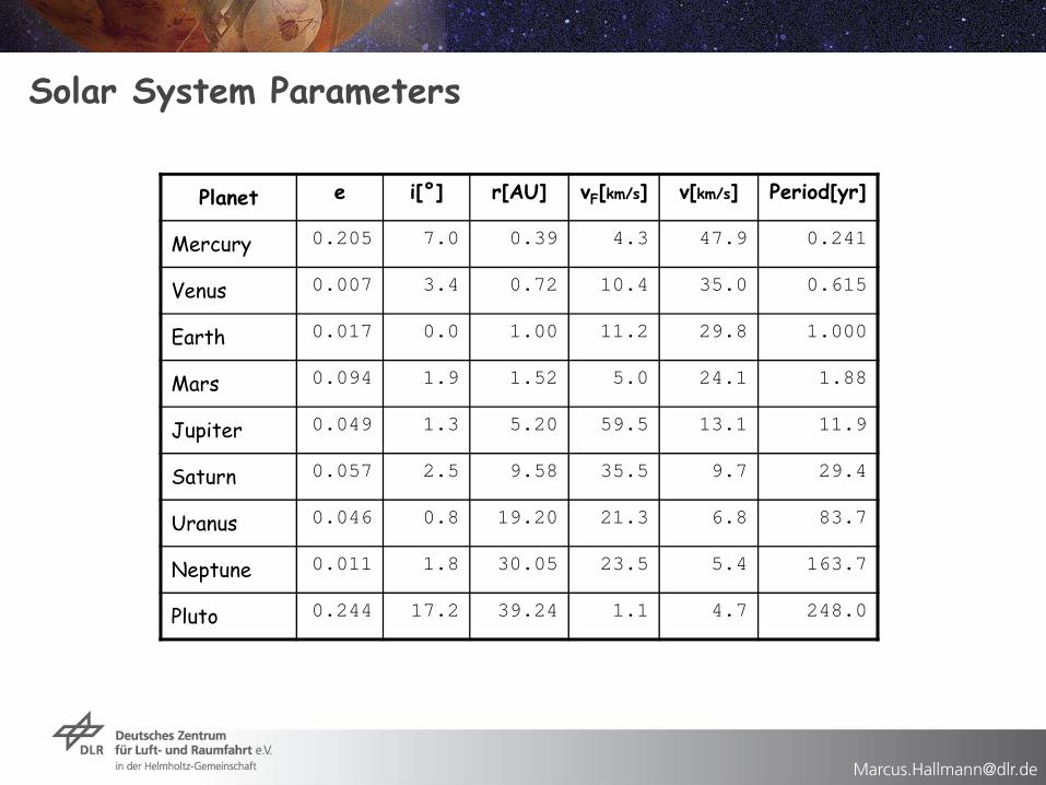
Solar System Parameters
Planet e i[°] r[AU] vF[km/s] v[km/s] Period[yr]
Mercury 0.205 7.0 0.39 4.3 47.9 0.241
Venus 0.007 3.4 0.72 10.4 35.0 0.615
Earth 0.017 0.0 1.00 11.2 29.8 1.000
Mars 0.094 1.9 1.52 5.0 24.1 1.88
Jupiter 0.049 1.3 5.20 59.5 13.1 11.9
Saturn 0.057 2.5 9.58 35.5 9.7 29.4
Uranus 0.046 0.8 19.20 21.3 6.8 83.7
Neptune 0.011 1.8 30.05 23.5 5.4 163.7
Pluto 0.244 17.2 39.24 1.1 4.7 248.0
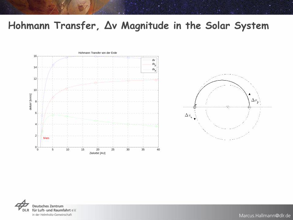
Hohmann Transfer, Δv Magnitude in the Solar System
0 5 10 15 20 25 30 35 400
2
4
6
8
10
12
14
16
Zielorbit [AU]
delta
V [k
m/s
]
Hohmann Transfer von der Erde
Mars
dvdvp
dva

Hohmann Transfer
0.2 0.4 0.6 0.8 1 1.2 1.4 1.60
5
10
15
20
25
Zielorbit [AU]
delta
V [k
m/s
]
Hohmann Transfer von der Erde
Mars
Venus
Merkur dvdvp
dva

Hohmann Transfer, Time-of-Flight
3
2
P at p
mD = =
Time-of-Flight:
( )1 23
1.52 1 1
2 2
+
Å
æ ö+ ÷ç= = ⋅ ÷ç ÷ç ÷è ø
r r
kPp
m
0.2 0.4 0.6 0.8 1 1.2 1.4 1.60.25
0.3
0.35
0.4
0.45
0.5
0.55
0.6
0.65
0.7
0.75
Zielorbit [AU]
Tran
sfer
zeit
[yr]
Hohmann Transfer von der Erde
Mars
VenusMerkur
0 5 10 15 20 25 30 35 400
5
10
15
20
25
30
35
40
45
50
Zielorbit [AU]
Tran
sfer
zeit
[yr]
Hohmann Transfer von der Erde
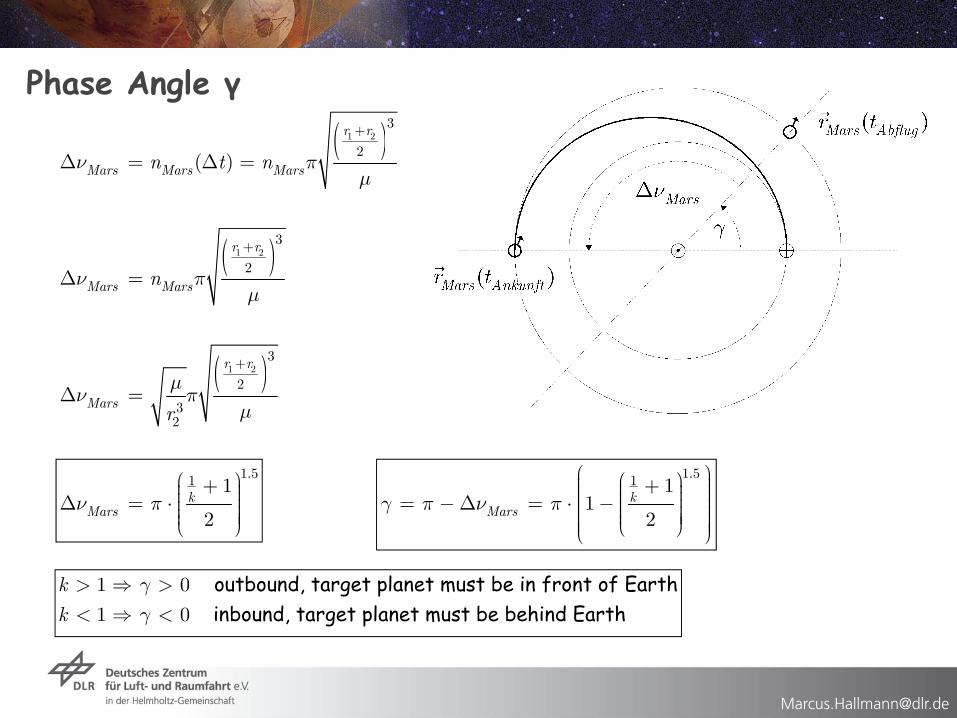
Phase Angle γ
( )1 23
2( )
+
D = D =
r r
Mars Mars Marsn t nn pm
( )1 23
2
+
D =
r r
Mars Marsnn pm
( )1 23
2
32
+
D =
r r
Marsr
mn p
m
1.51 1
2
æ ö+ ÷ç ÷çD = ⋅ ÷ç ÷ç ÷÷çè ø
kMarsn p
1.51 11
2
æ öæ ö ÷ç + ÷÷çç ÷÷çç= - D = ⋅ - ÷÷çç ÷÷çç ÷÷÷çç ÷è ø ÷çè ø
kMarsg p n p
1 0
1 0
k
k
gg
> >< <
outbound, target planet must be in front of Earthinbound, target planet must be behind Earth
0 5 10 15 20 25 30 35 40-300
-250
-200
-150
-100
-50
0
50
100
150
Zielorbit [AU]
Pha
senw
inke
l [d
eg]
Hohmann Transfer von der Erde
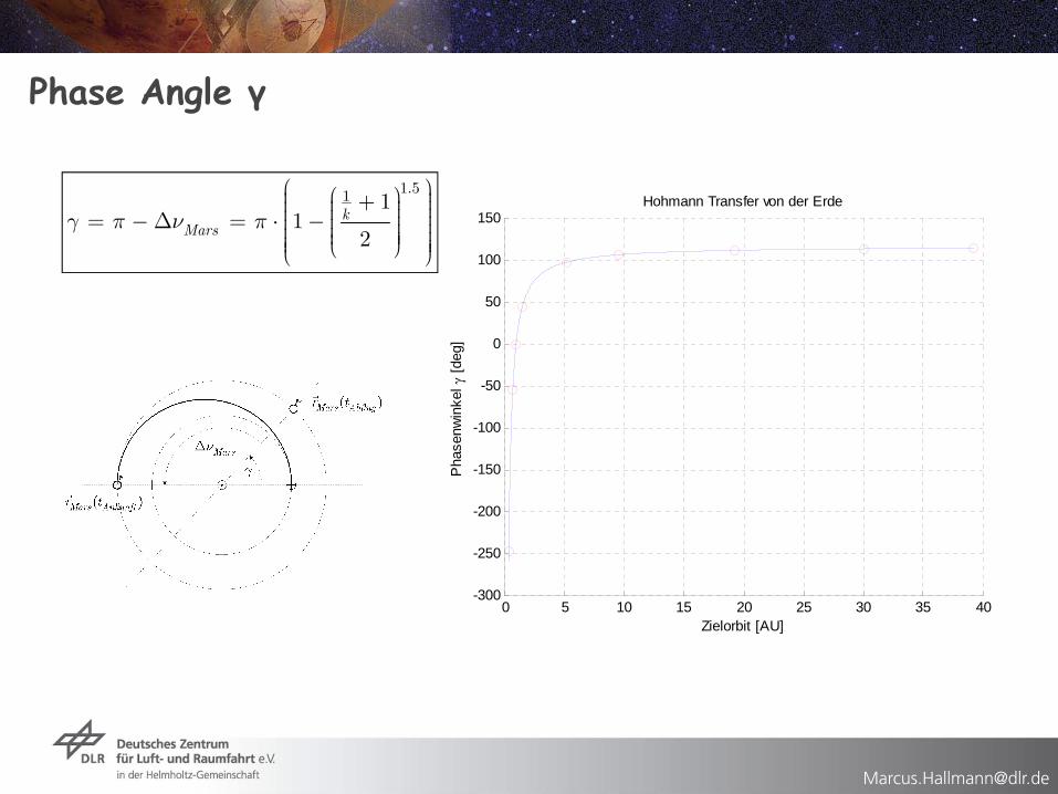
Phase Angle γ
1.51 11
2
æ öæ ö ÷ç + ÷÷çç ÷÷çç= - D = ⋅ - ÷÷çç ÷÷çç ÷÷÷çç ÷è ø ÷çè ø
kMarsg p n p
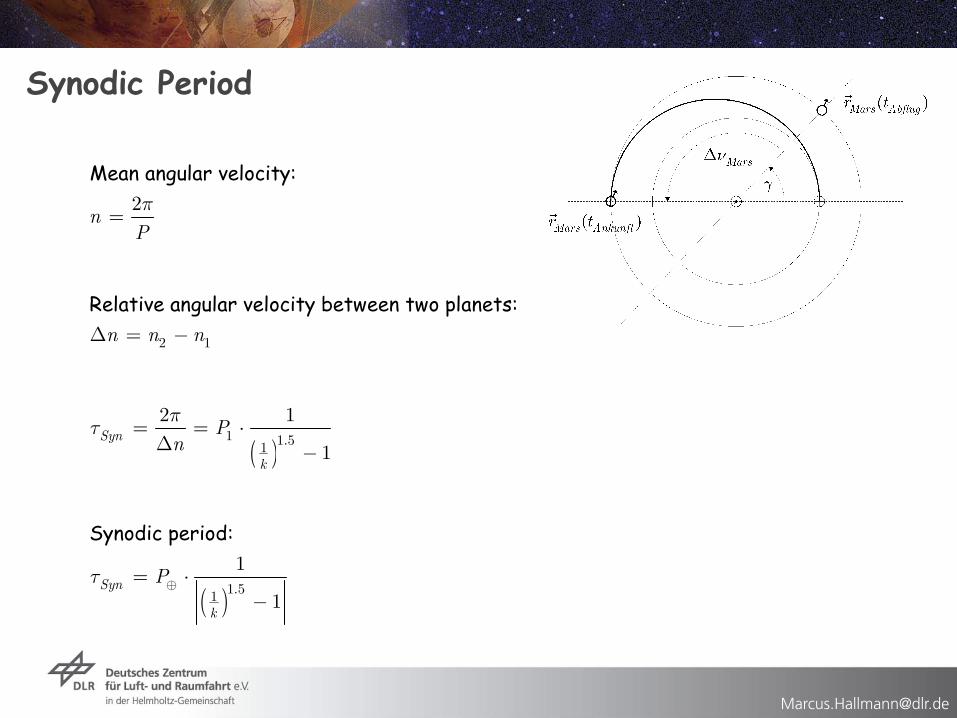
Synodic Period
2n
P
p=
Mean angular velocity:
( )1 1.51
2 1
1Syn
k
Pn
pt = = ⋅
D -
2 1n n nD = -Relative angular velocity between two planets:
( )1.51
1
1Syn
k
Pt Å= ⋅-
Synodic period:
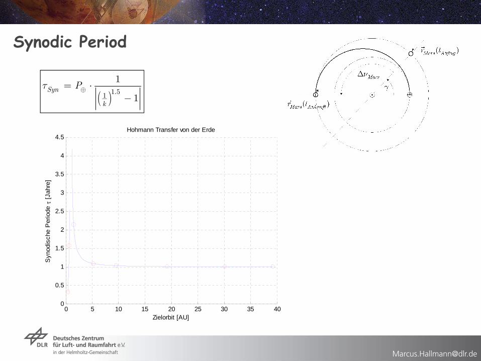
Synodic Period
0 5 10 15 20 25 30 35 400
0.5
1
1.5
2
2.5
3
3.5
4
4.5
Zielorbit [AU]
Syn
odis
che
Per
iode
[J
ahre
]
Hohmann Transfer von der Erde
( )1.51
1
1Å= ⋅
-Syn
k
Pt
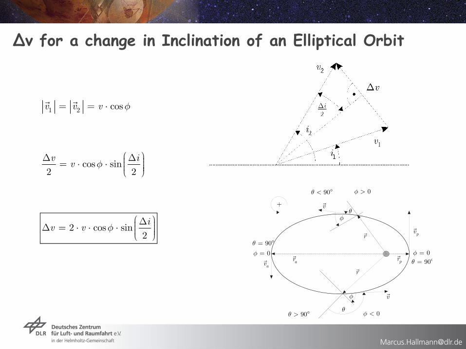
Δv for a change in Inclination of an Elliptical Orbit
1 2 cos= = ⋅ v v v f
cos sin2 2
æ öD D ÷ç= ⋅ ⋅ ÷ç ÷ç ÷è øv i
v f
2 cos sin2
æ öD ÷çD = ⋅ ⋅ ⋅ ÷ç ÷ç ÷è øi
v v f
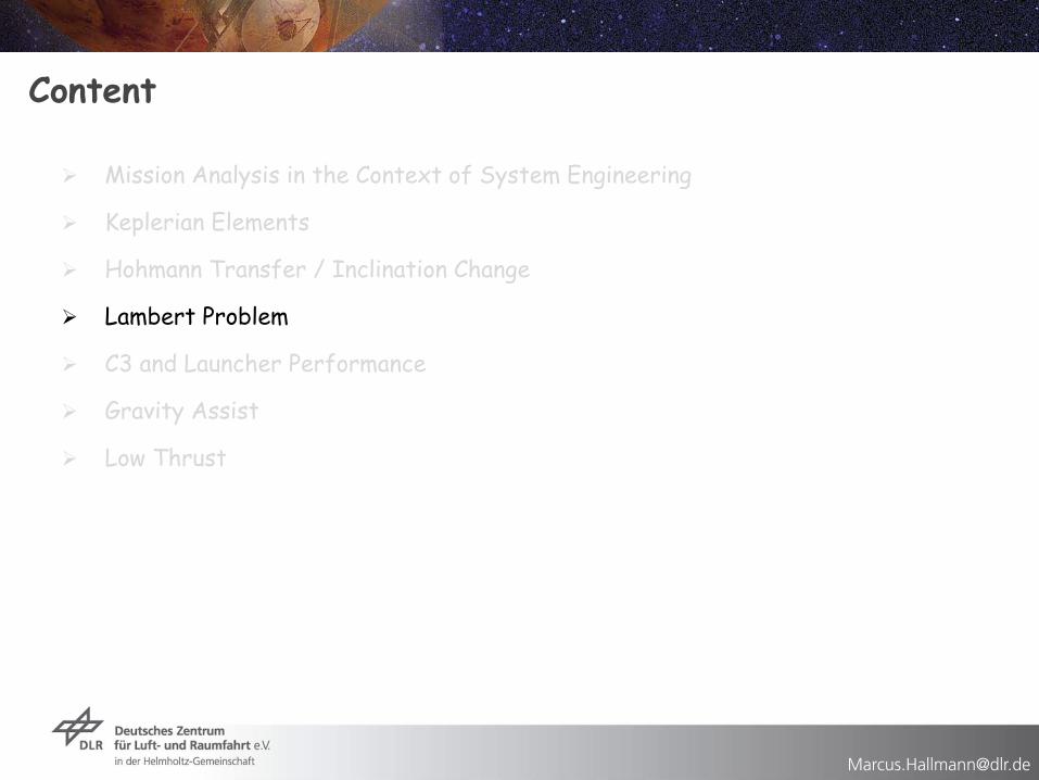
Content
Mission Analysis in the Context of System Engineering
Keplerian Elements
Hohmann Transfer / Inclination Change
Lambert Problem
C3 and Launcher Performance
Gravity Assist
Low Thrust
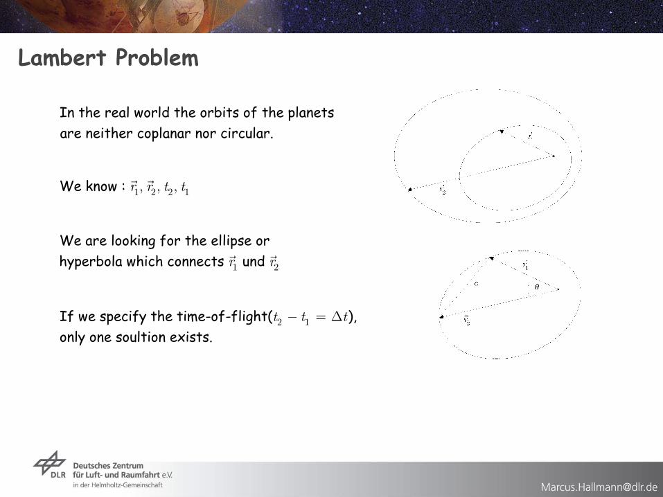
Lambert Problem
1 2 2 1, , ,r r t t We know :
1 2r r
We are looking for the ellipse or hyperbola which connects und
In the real world the orbits of the planets are neither coplanar nor circular.
2 1t t t- = DIf we specify the time-of-flight( ), only one soultion exists.
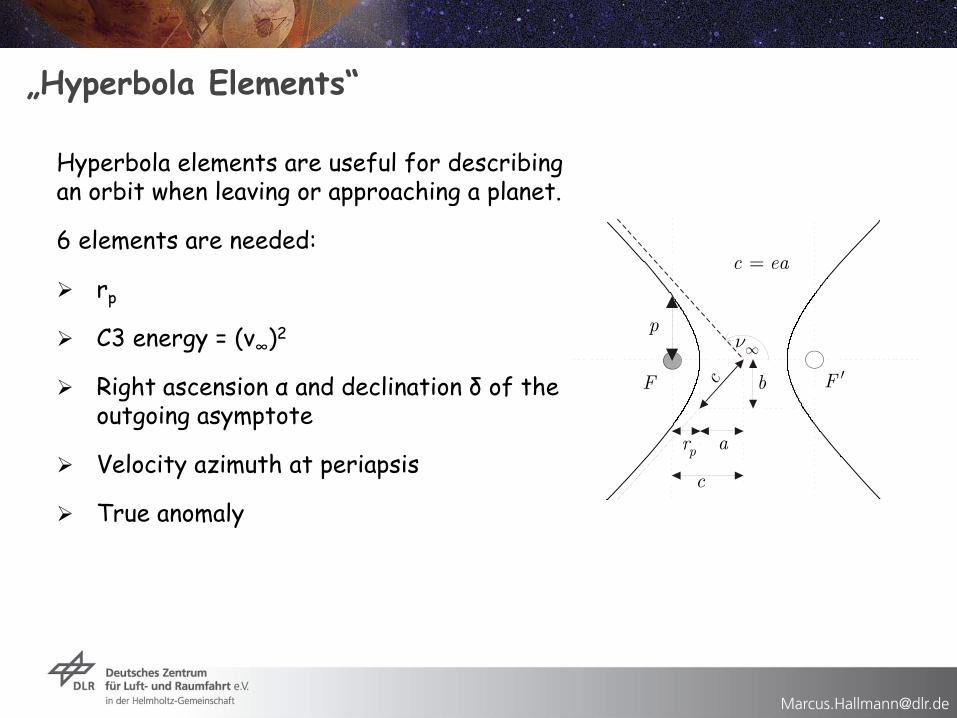
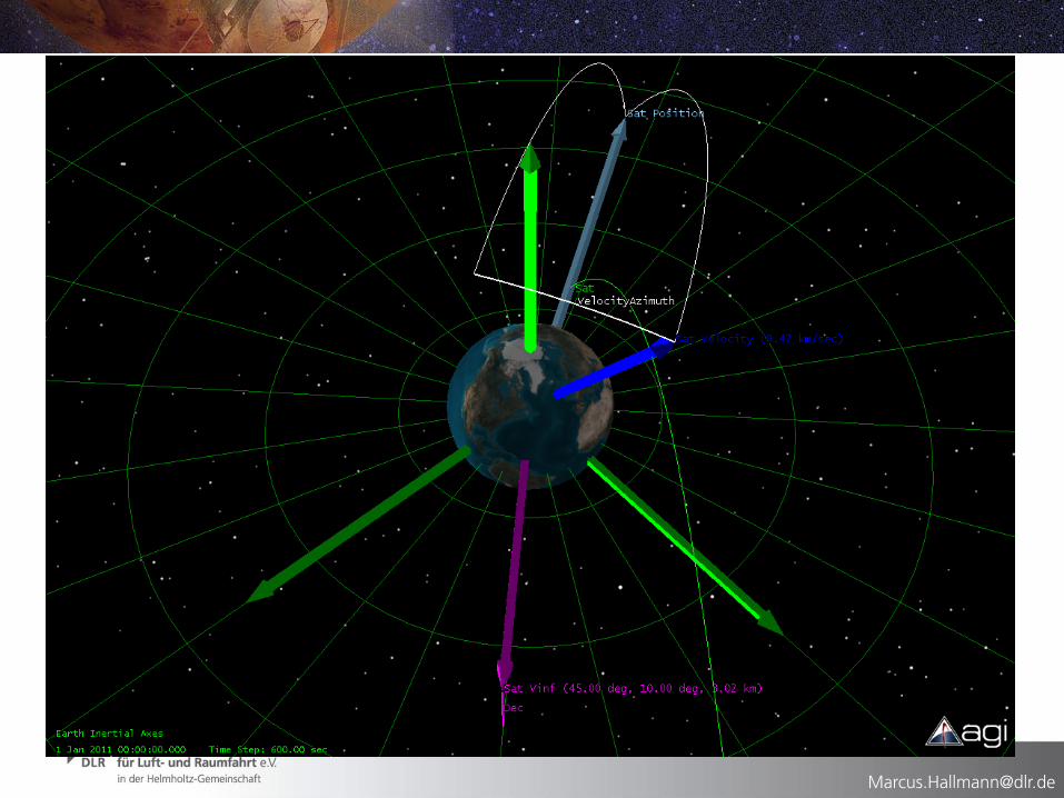
„Hyperbola Elements“
Hyperbola elements are useful for describing an orbit when leaving or approaching a planet.
6 elements are needed:
rp
C3 energy = (v∞)2
Right ascension α and declination δ of theoutgoing asymptote
Velocity azimuth at periapsis
True anomaly
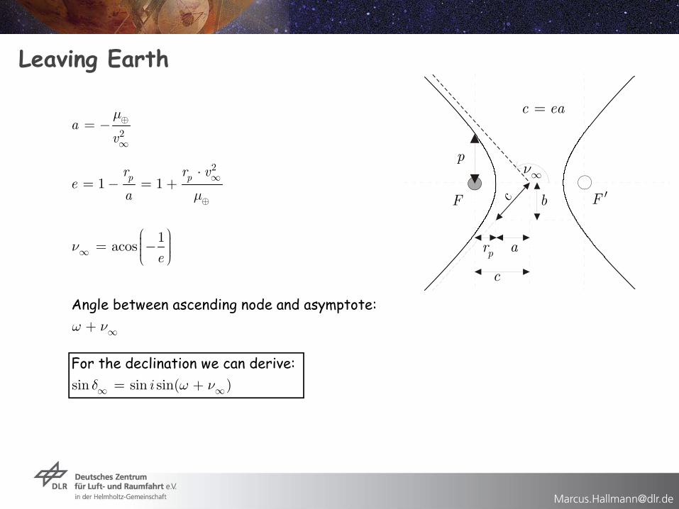
Leaving Earth
2a
v
mÅ
¥
= -
2
1 1p pr r ve
a m¥
Å
⋅= - = +
1acos
en¥
æ ö÷ç= - ÷ç ÷ç ÷è ø
w n¥+Angle between ascending node and asymptote:
sin sin sin( )i w nd¥ ¥= +For the declination we can derive:
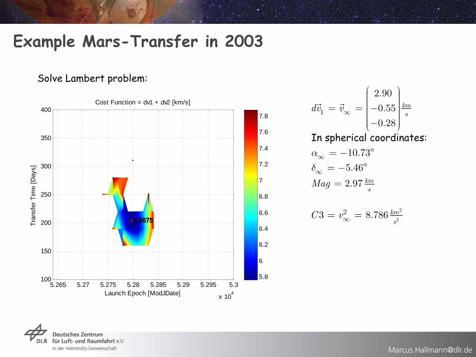
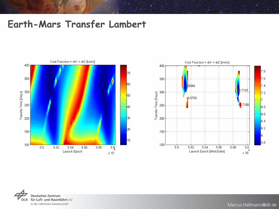
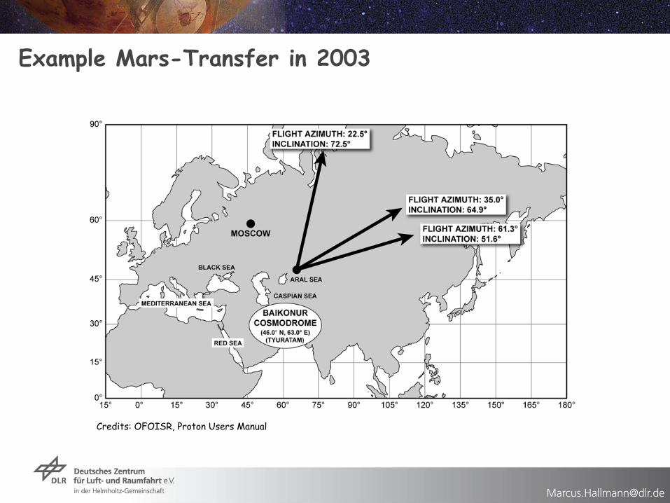
Example Mars-Transfer in 2003
Solve Lambert problem:
Launch Epoch [ModJDate]
Tran
sfer
Tim
e [D
ays]
Cost Function = dv1 + dv2 [km/s]
5.6675 5.6675 5.6675 5.6675 5.6675 5.6675 5.6675 5.6675 5.6675 5.6675
5.265 5.27 5.275 5.28 5.285 5.29 5.295 5.3
x 104
100
150
200
250
300
350
400
5.8
6
6.2
6.4
6.6
6.8
7
7.2
7.4
7.6
7.8
2
2
1
2
2.90
0.55
0.28
10.73
5.46
2.97
3 8.786
kms
kms
kms
dv v
Mag
C v
ad
¥
¥
¥
¥
æ ö÷ç ÷ç ÷ç ÷ç= = - ÷ç ÷ç ÷÷ç- ÷çè ø
= - = -
=
= =
In spherical coordinates:
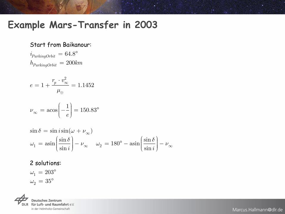
Example Mars-Transfer in 2003
2
1 1.1452pr ve
m¥
Å
⋅= + =
1acos 150.83
en¥
æ ö÷ç= - ÷ = ç ÷ç ÷è ø
1 2
sin sin sin( )
sin sinasin 180 asin
sin sin
i
i i
d w nd d
w n w n
¥
¥ ¥
= +æ ö æ ö÷ ÷ç ç= ÷ - = - ÷ -ç ç÷ ÷ç ç÷ ÷è ø è ø
64.8
200ParkingOrbit
ParkingOrbit
i
h km
= =
Start from Baikanour:
1
2
203
35
ww
= =
2 solutions:
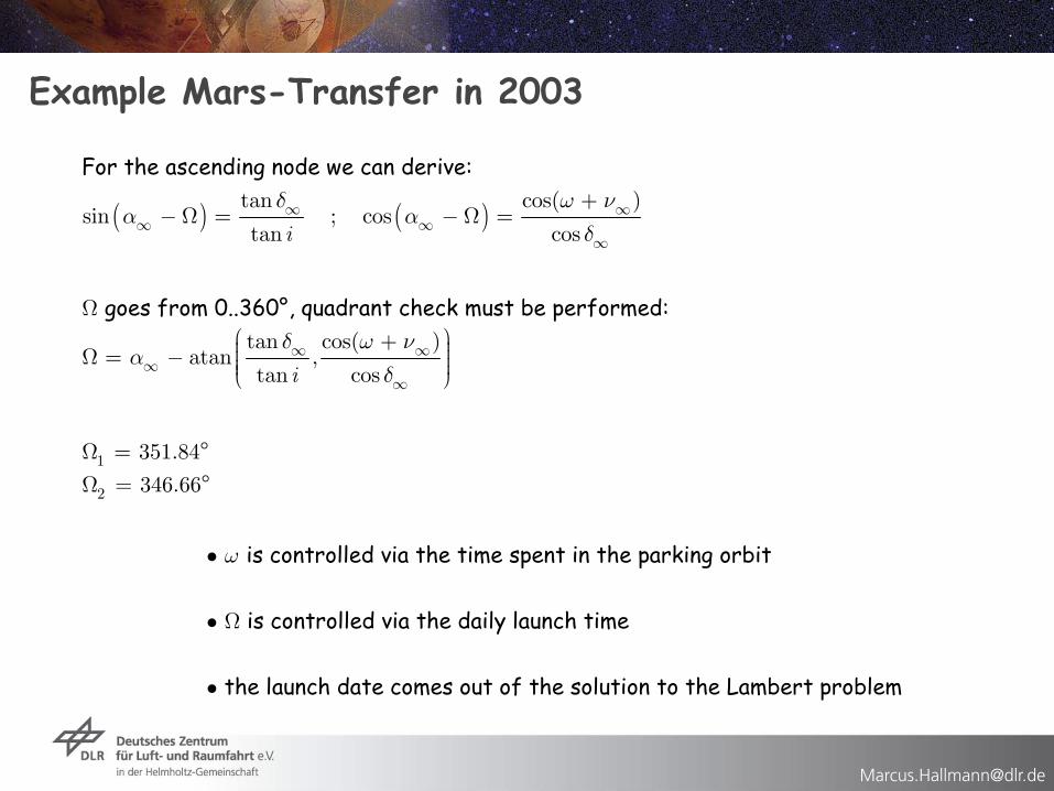
Example Mars-Transfer in 2003
( ) ( )tan cos( )sin ; cos
tan cosi
d w na a
d¥ ¥
¥ ¥¥
+-W = -W =
For the ascending node we can derive:
tan cos( )atan ,
tan cosi
d w na
d¥ ¥
¥¥
Wæ ö+ ÷ç ÷W = - ç ÷ç ÷çè ø
goes from 0..360°, quadrant check must be performed:
1
2
351.84
346.66
W = W =
w·
· W
·
is controlled via the time spent in the parking orbit
is controlled via the daily launch time
the launch date comes out of the solution to the Lambert problem
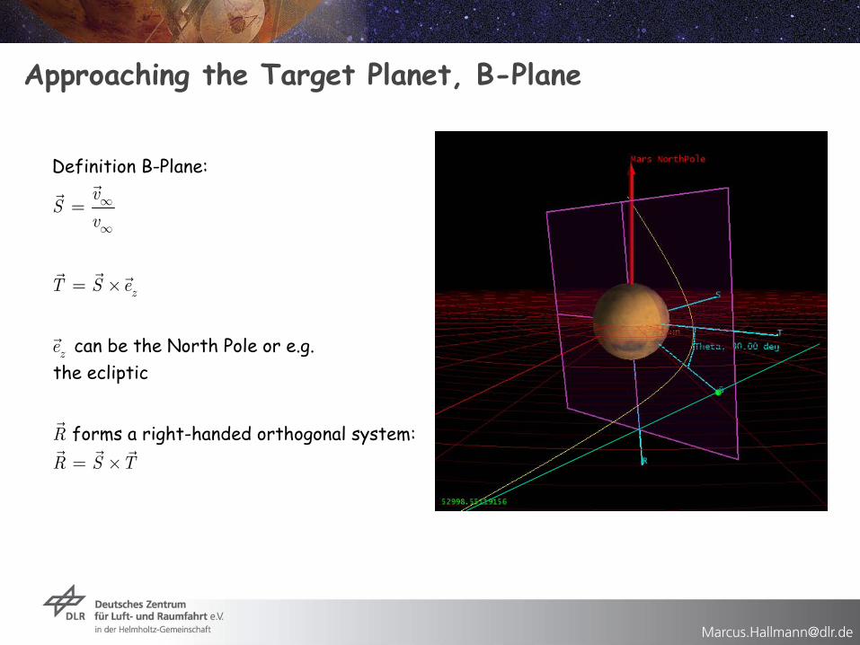
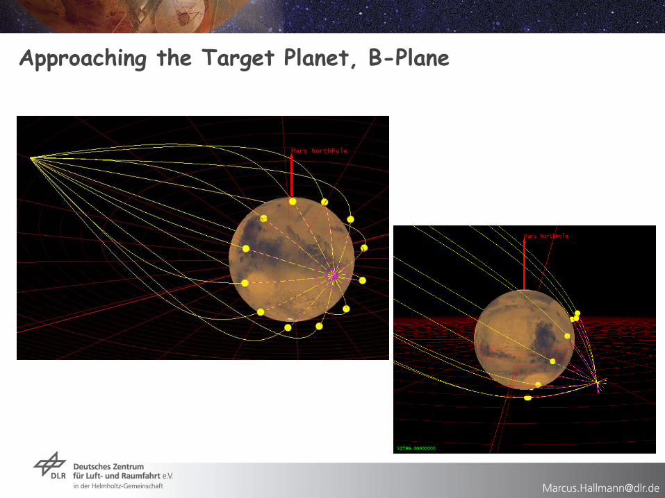
Approaching the Target Planet, B-Plane
vS
v¥
¥
=
Definition B-Plane:
zT S e= ´
ze can be the North Pole or e.g. the ecliptic
R
R S T= ´
forms a right-handed orthogonal system:
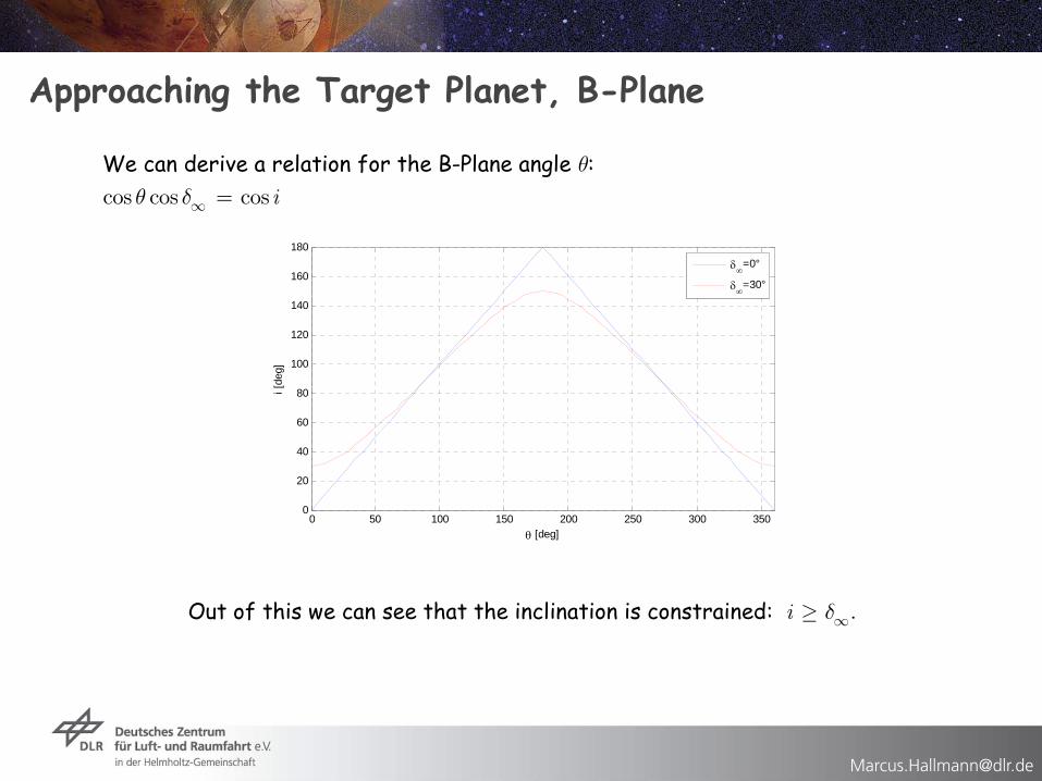
Approaching the Target Planet, B-Plane
cos cos cos i
qq d¥ =
We can derive a relation for the B-Plane angle :
.i d¥³Out of this we can see that the inclination is constrained:
0 50 100 150 200 250 300 3500
20
40
60
80
100
120
140
160
180
[deg]
i [de
g]
=0°
=30°

Content
Mission Analysis in the Context of System Engineering
Keplerian Elements
Hohmann Transfer / Inclination Change
Lambert Problem
C3 and Launcher Performance
Gravity Assist
Low Thrust
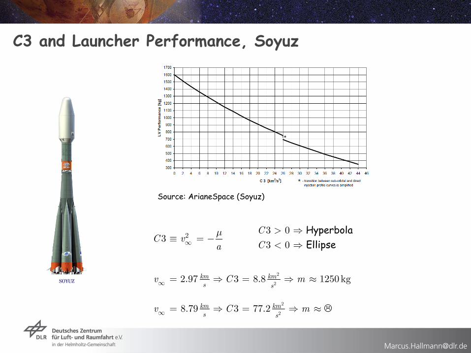
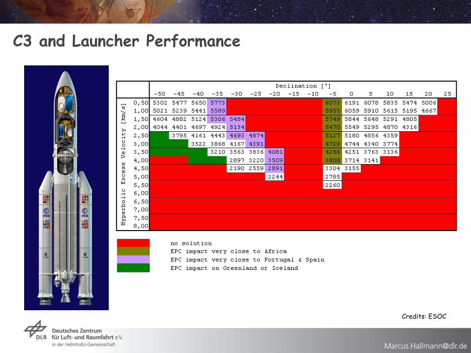
C3 and Launcher Performance, Soyuz
Source: ArianeSpace (Soyuz)
23C va
m¥º = -
2
22.97 3 8. 1258 0kgkm km
s sv mC¥ = = »
3 0
3 0
C
C
> <
HyperbolaEllipse
2
28.79 3 77.2km km
s sCv m¥ == »
Content
Mission Analysis in the Context of System Engineering
Keplerian Elements
Hohmann Transfer / Inclination Change
Lambert Problem
C3 and Launcher Performance
Gravity Assist
Low Thrust
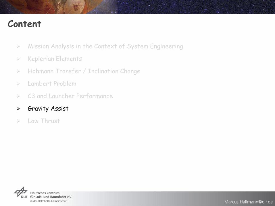
Gravity Assist 2D Case
2
1cos
1
)(
peri
Planet
er v
e
n
m
¥
¥
= -
⋅= +
12 arcsin
ea
æ ö÷ç= ⋅ ÷ç ÷ç ÷è ø
Deflection angle:
( )v va¥- ¥+= ⋅Rot
12 ¥D = ⋅Satv v
e
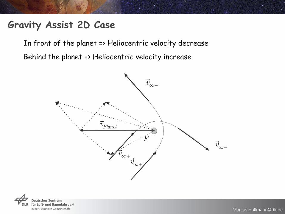
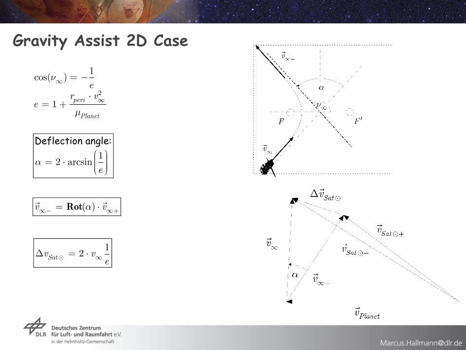
Gravity Assist 2D Case
In front of the planet => Heliocentric velocity decrease
Behind the planet => Heliocentric velocity increase
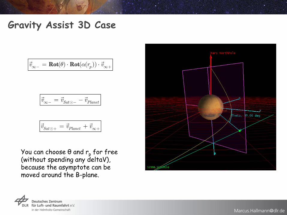
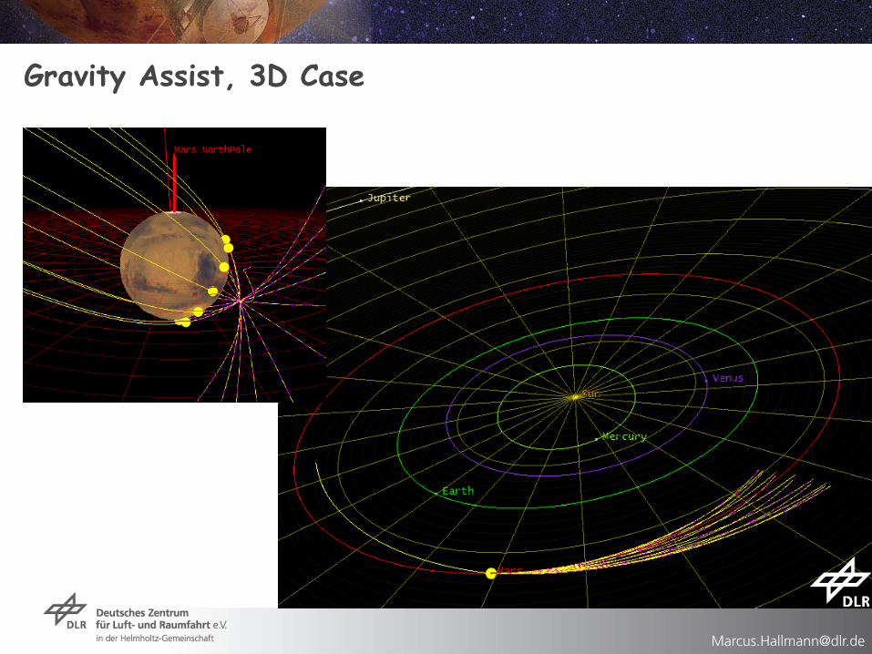
Gravity Assist 3D Case
( ) ( ( ))pv r vq a¥- ¥+= ⋅ ⋅Rot Rot
Sat Planetv v v¥- -= -
Sat Planetv v v+ ¥+= +
You can choose θ and rp for free(without spending any deltaV), because the asymptote can bemoved around the B-plane.
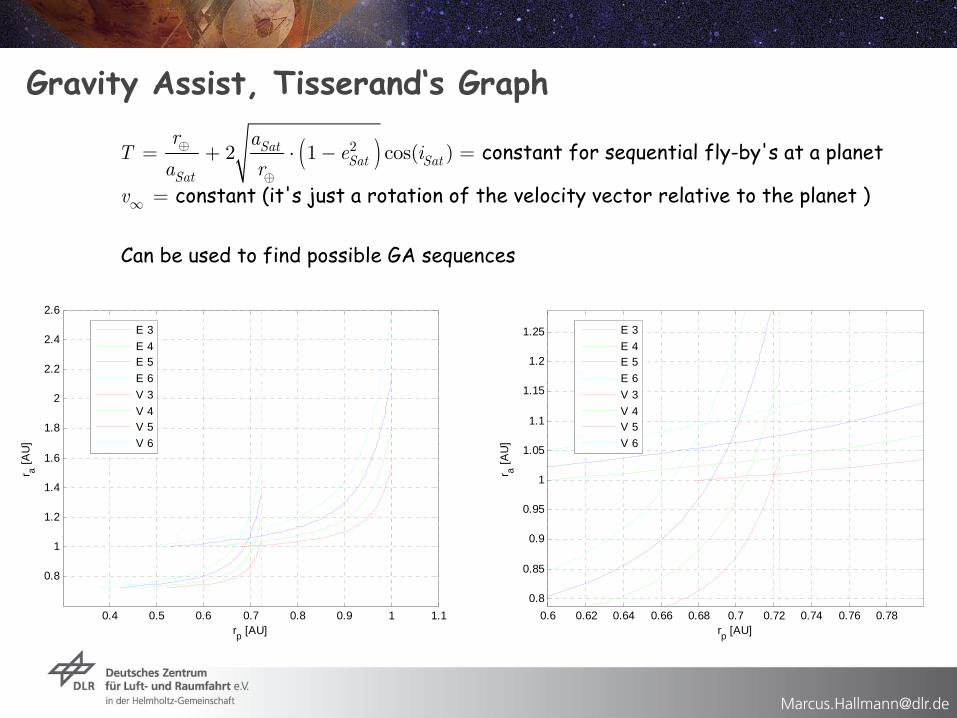
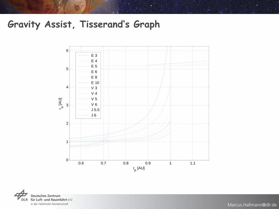
Gravity Assist, Tisserand‘s Graph
( )22 1 cos( )SatSat Sat
Sat
v
r aT e i
a rÅ
Å
¥
= + ⋅ - =
=
constant for sequential fly-by's at a planet
constant (it's just a rotation of the velocity vector relative to the planet )
Can be used to find possible GA sequences
0.4 0.5 0.6 0.7 0.8 0.9 1 1.1
0.8
1
1.2
1.4
1.6
1.8
2
2.2
2.4
2.6
rp [AU]
r a [AU
]
E 3E 4E 5E 6V 3V 4V 5V 6
0.6 0.62 0.64 0.66 0.68 0.7 0.72 0.74 0.76 0.780.8
0.85
0.9
0.95
1
1.05
1.1
1.15
1.2
1.25
rp [AU]
r a [AU
]
E 3E 4E 5E 6V 3V 4V 5V 6
Gravity Assist, Tisserand‘s Graph
0.6 0.7 0.8 0.9 1 1.10
1
2
3
4
5
6
rp [AU]
r a [AU
]
E 3E 4E 5E 6E 8E 10V 3V 4V 5V 6J 5.5J 6
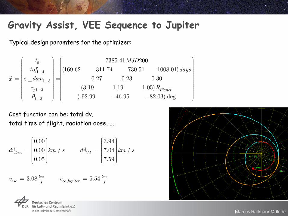
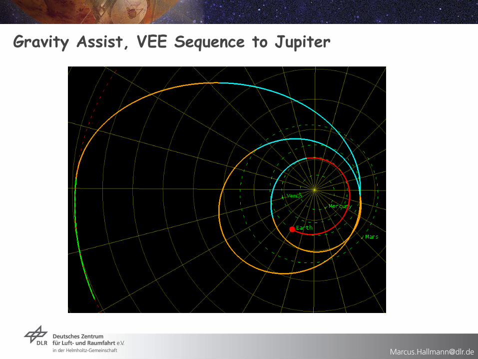
Gravity Assist, VEE Sequence to Jupiter
0
1...4
1...3
1...3
1...3
7385.41 200
(169.62 311.74 730.51 1008.01)
_ 0.27 0.2
p
t MJD
tof days
dsmx
r
e
q
æ ö÷ç ÷ç ÷ç ÷ç ÷ç ÷ç ÷÷ç= =÷ç ÷ç ÷ç ÷ç ÷ç ÷ç ÷ç ÷÷çè ø
Typical design paramters for the optimizer:
3 0.30
(3.19 1.19 1.05)
(-92.99 - 46.95 - 82.03) degPlanetR
æ ö÷ç ÷ç ÷ç ÷ç ÷ç ÷ç ÷÷ç ÷ç ÷ç ÷ç ÷ç ÷ç ÷ç ÷ç ÷÷çè ø
Cost function can be: total dv, total time of flight, radiation dose, ...
0.00 3.94
0.00 / 7.04 /
0.05 7.59dsm GAdv km s dv km s
æ ö æ ö÷ ÷ç ç÷ ÷ç ç÷ ÷ç ç÷ ÷ç ç= =÷ ÷ç ç÷ ÷ç ç÷ ÷÷ ÷ç ç÷ ÷ç çè ø è ø
3.08 5.54km kmesc Jupiters s
v v¥= =

Gravity Assist, Tisserand‘s Graphs, Jupiter System
0.4 0.6 0.8 1 1.2 1.4 1.6 1.8 2
x 106
0
5
10
15
20
25
30
35
40
45
50
rp [km]
Per
iod
[day
s]
E G C
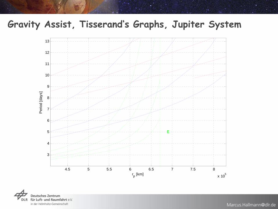
Gravity Assist, Tisserand‘s Graphs, Jupiter System
4.5 5 5.5 6 6.5 7 7.5 8
x 105
3
4
5
6
7
8
9
10
11
12
13
rp [km]
Per
iod
[day
s]
E
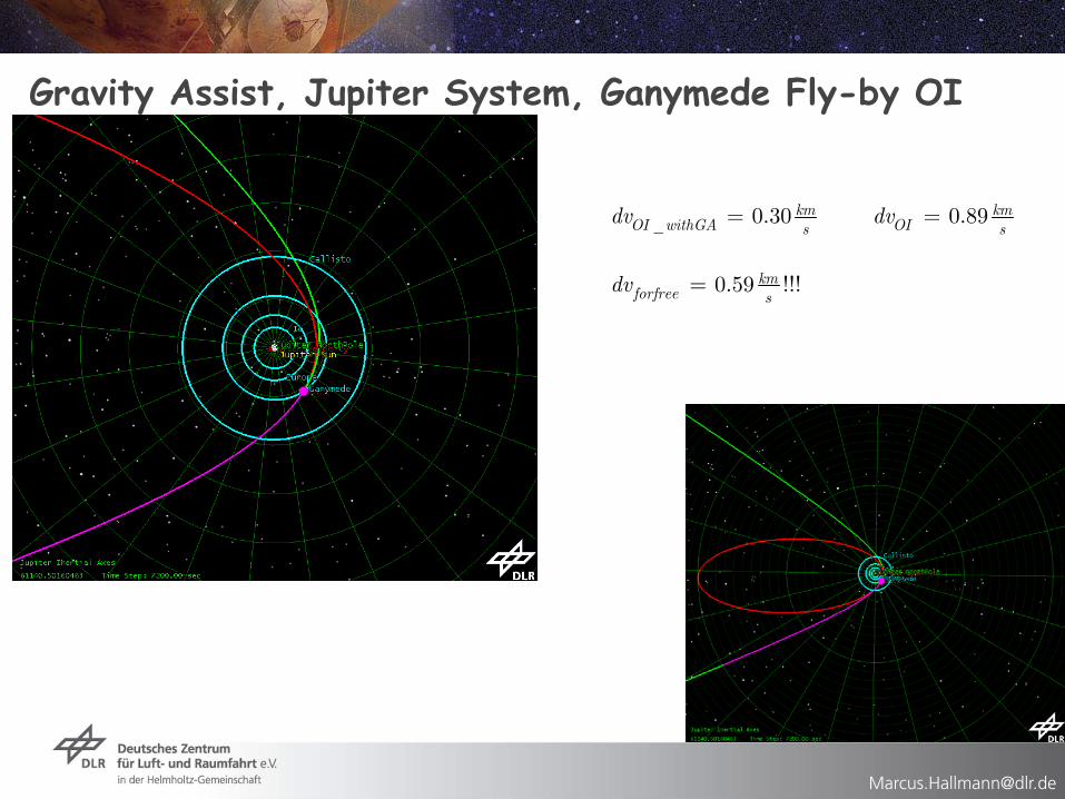
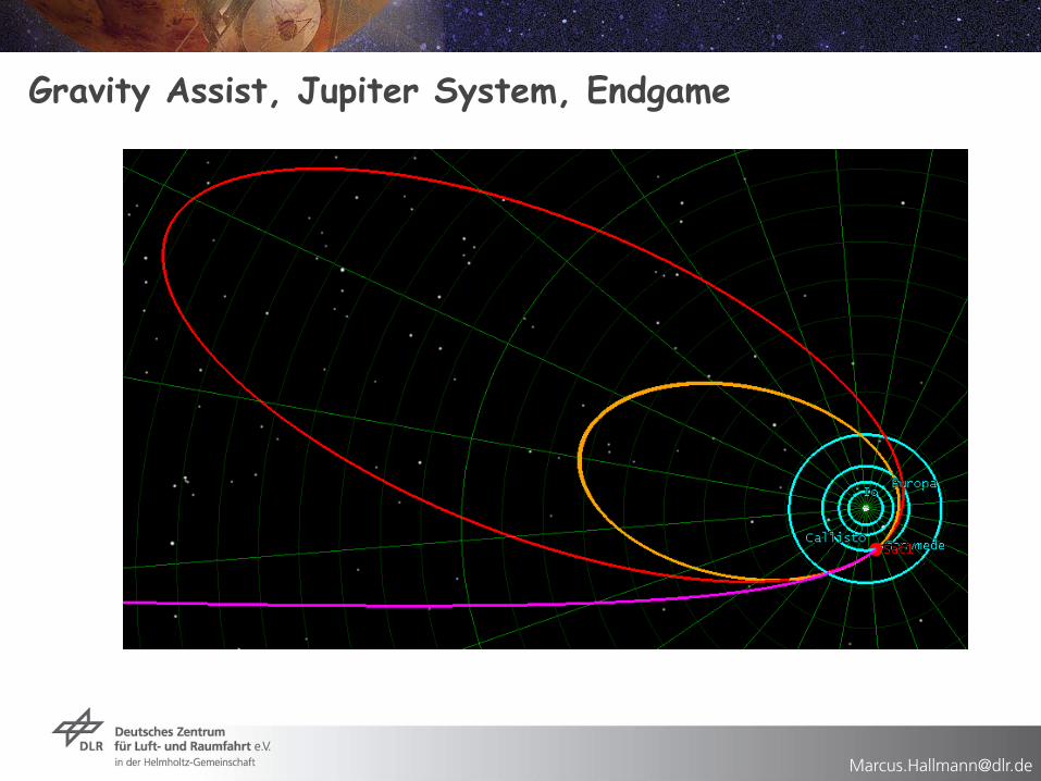
Gravity Assist, Jupiter System, Ganymede Fly-by OI
_ 0.30 0.89
0.59 !!!
km kmOI withGA OIs s
kmforfree s
dv dv
dv
= =
=
Content
Mission Analysis in the Context of System Engineering
Keplerian Elements
Hohmann Transfer / Inclination Change
Lambert Problem
C3 and Launcher Performance
Gravity Assist
Low Thrust
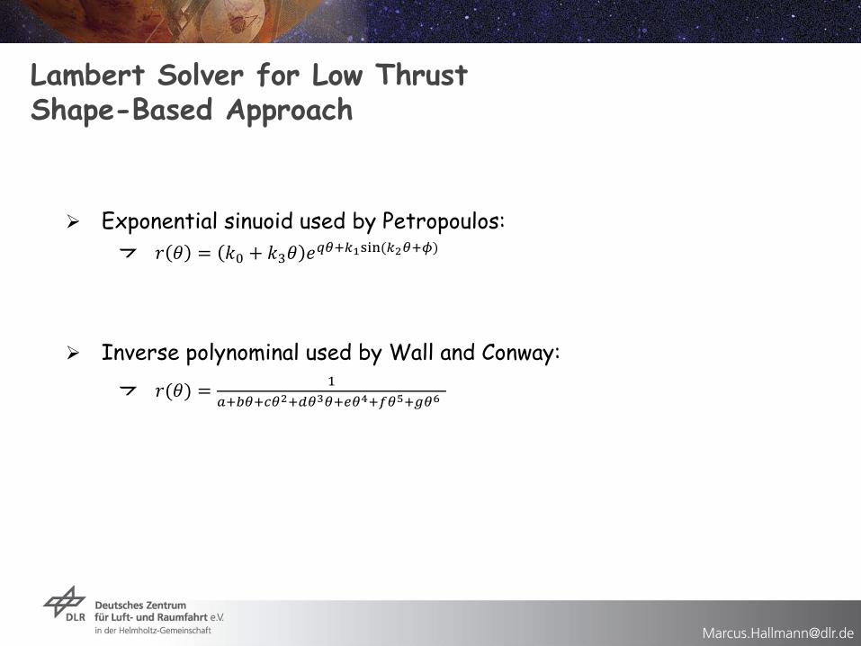
Lambert Solver for Low ThrustShape-Based Approach
Exponential sinuoid used by Petropoulos:
Inverse polynominal used by Wall and Conway:
Literatur
Interplanetary Mission Analysis and Design, Stephen KembleISBN 3-540-29913-0
Fundamentals of Astrodynamics and Applications, David ValladoISBN 978-1881883142
Space Mission Engineering: The new SMAD, James R. WertzISBN 978-1-881-883-15-9
Deep Space Craft, An overview of Interplanetary Flight, Dave DoodyISBN 978-3-540-89509

Web
http://sourceforge.net/projects/pagmo/
http://keptoolbox.sourceforge.net/
http://nssdc.gsfc.nasa.gov/planetary/planetfact.html
http://naif.jpl.nasa.gov/naif/spiceconcept.html