OPTIMAL ORDERING IN SEQUENTIAL

ENGLISH AUCTIONS:

A REVENUE-COMPARISON MODEL FOR 18TH CENTURY ART AUCTIONS IN LONDON AND

PARIS

AMAAN AMJAD MITHA

PROFESSOR NEIL DE MARCHI, FACULTY ADVISOR

Honors Thesis submitted in partial fulfillment of the requirements for Graduation with

Distinction in Economics in Trinity College of Duke University.

Duke University

Durham, North Carolina

2012

2

ACKNOWLEDGEMENTS

Professor De Marchi, thank you for all of your help, support, and guidance.

You’ve been a fantastic advisor, and your enthusiasm has been inspiring. Professor Van

Miegroet, thank you for all of your advice and support, and for introducing me to

DALMI and the trailblazing work you’re doing; I’m happy to have been a part of it, and

I’m excited to see what’s in store. Ms. Benedicte Miyamoto-Pavot and Ms. Hilary Coe

Smith, thank you both for providing me your data; I know how closely-guarded PhD

data is, and I appreciate all that you did to get me access. Professor Roberts, thank you

for all of your helpful insights and suggestions, you helped me focus my study and my

attention to specific issues. Finally, to my family and my friends: thank you for putting

up with the absurd hours and the cantankerousness that naturally accompany an

undertaking of this magnitude.

3

TABLE OF CONTENTS

Acknowledgements ..................................................................................................................... 2

Abstract.......................................................................................................................................... 5

I. Introduction ........................................................................................................................... 6

II. Background and Literature Review ................................................................................. 10

III. Model ................................................................................................................................ 17

A. Revenue Normalization ................................................................................................. 18

B. Value Declination Normalization ................................................................................. 20

C. Testable Model ................................................................................................................ 23

IV. Data ................................................................................................................................... 24

A. Paris Database ................................................................................................................. 24

B. Christie’s Database ......................................................................................................... 27

V. Results .................................................................................................................................. 28

A. Paris Results ..................................................................................................................... 29

B. Christie’s Results ............................................................................................................. 31

VI. Conclusions ...................................................................................................................... 34

References ................................................................................................................................... 36

4

Appendices ................................................................................................................................. 40

A. Collection of Paris Auction Data .................................................................................. 40

B. Bias in Price as a Proxy for Value ................................................................................. 42

C. Test for Regularity in Value vs. Lot Order .................................................................. 43

5

ABSTRACT

We develop a model based on several auction parameters to test the widely held

notion that in a sequential English auction, it is optimal for the seller to arrange the lots

in order of decreasing value. We test this model against two datasets of 18th century

auctions, one of various auctions from Paris and the other from Christie’s sales in

London. We find that the Paris data support the claim, while the Christie’s data seem to

refute the optimal strategy. We also find a rationale for bidders in the Christie’s

auctions to alter their strategies, accounting for the discrepancy.

JEL Classifications: D44, Z11

Keywords: Auctions, Lot Ordering, Optimal Auction Strategy, English Auction,

Sequential Auctions

6

I. INTRODUCTION

The concept of the auction has existed for several millennia. The first recorded

mention of the auction comes from Herodotus, who tells us that auctions occurred as

long ago as the 5th century BC. Historically, auctions have been used to sell all manner

of objects, from people (wives and slaves) to entire empires; at one point the Praetorian

Guard killed the sitting emperor and auctioned off the Roman Empire (McAfee &

McMillan, 1987, p. 701; Krishna, 2002, p. 1). Today, auctions are more widely used than

ever before, from the sale of physical commodities to art to public resources to debt.

Trading securities can even be modeled as a continuous sequential auction of common

value goods (Kyle, 1985), hence the use of the term “bid” for a price offer. The benefit

of using an auction is that it is an efficient way of determining the value of an object

with an inherently indeterminate value. A seller wants to get rid of some object, but

does not know how to appropriately assign a price to it. So, if he devises a suitable

auction mechanism, he can sell the object to the person who values it most, benefitting

both the seller and the buyer.

Today, there are four generally recognized auction formats. These are the

following:

(1) Open Ascending Price Auction (English);

(2) Open Descending Price Auction (Dutch);

7

(3) Sealed-Bid First-Price Auction;

(4) Sealed-Bid Second-Price Auction.

There are several variants on each of these, but they are widely considered the four

standard formats.

The English auction is by far the most common format in use today (McAfee &

McMillan, 1987, p. 702); when most people imagine an auction, they are thinking of the

English form. Essentially, an English auction can be described with the following

scenario. An object is put up for auction, and bidders openly offer competing bids.

These bids must increase, and the object is finally sold to the last remaining bidder. He

must pay the amount at which his final competitor dropped out (Krishna, 2002, p. 2).

This is the format generally used in art auctions today, and it is the format of the

auctions studied in this paper.

The Dutch auction is the descending price foil to the English auction. The

auctioneer starts the bidding at a value far higher than any bidder’s valuation, and he

steadily decreases the bid until a bidder agrees to buy at that price. This bidder wins

the object, and must pay the agreed-upon price. This format is rarely used today, but

was used to sell cut flowers in the Netherlands, hence the name. It has also been used

in sales of perishable commodities, like fish and tobacco (McAfee & McMillan, 1987, p.

702).

8

The sealed-bid first-price auction operates as follows: bidders offer their

competing bids in sealed envelopes, and whoever offers the highest bid wins; he must

then pay his bid (or in the case of a contract, the lowest bid wins). The sealed-bid

second-price auction is set up similarly, but instead of paying his own bid, the winner

pays the second-highest bid. Sealed-bid first-price auctions are used for such objects as

government contracts and mineral rights on public lands (McAfee & McMillan, 1987, p.

702). The sealed-bid second-price auction was originally a theoretical development

published by Vickrey (1961), but it has come into use in modern times. For example, on

eBay, a bidder can submit his maximum bid, and if it is the highest valuation at the end

of the auction, he must pay only $0.01 more than the second-highest bid.

One of the issues that must be considered in auction theory is the way in which a

bidder values an object at auction. There are two distinct possibilities, private versus

common value. In a private values context, each bidder assigns his own valuation to

the object independent of the other bidders’ valuations. Private values makes sense

when modeling objects that are used solely for consumption. In a common values (or

“interdependent” values) setting, the object has some unique value; the reason that an

auction is necessary is that nobody actually knows this true value, though each bidder

has his own estimate. This is a useful model for goods that can be resold, like securities

or plots of land with unknown mineral content (Krishna, 2002, pp. 3-4). In this

situation, the bidders’ valuations represent estimates of the true value. One result of a

9

common values auction with incomplete information is the so-called winner’s curse, in

which the bidder with the highest valuation overestimates the value of the object. It

can, however, be avoided by using an equilibrium bidding strategy (Krishna, 2002, p.

85).

Unfortunately, art is neither a consumption good nor an investment good; it falls

in that murky space somewhere in between. This makes modeling art auctions

somewhat more difficult, as theorists must choose ex ante which valuation model they

deem appropriate. In the case of this study, it turns out that either valuation model

(private or common) offers the same hypothesis: the seller’s optimal strategy is to sell

objects in a sequential English auction in order of decreasing value. This is a notion

supported by both theory and empirical study (see II. Background and Literature Review).

Tests of this claim have focused solely on recent auctions, despite the fact that

institutional auctions have been used in sales of artwork since the 18th century. This

study offers a test of the optimal hypothesis using historical records. This allows us to

discern whether the claim holds up in auctions that occurred prior to the theoretical

developments, confirming that modern empirical agreement with the theory is not a

result of auction houses utilizing that same theory. We do this by developing a model

that allows us to compare the auction revenues with the degree to which values

declined over the course of a specific auction.

10

II. BACKGROUND AND LITERATURE REVIEW

Since Vickrey’s seminal work, “Counterspeculation, Auctions, and Competitive

Sealed Tenders, ” there has been a steady stream of research in auctions, in the context

of both theory and practice. Vickrey’s (1961) groundbreaking discovery was the fact

that under his model, the Dutch auction was strategically equivalent to the sealed-bid

first-price auction, and the English auction was weakly equivalent to the sealed-bid

second price auction. This led him to discover that the auctioneer’s expected revenue

for a first-price sealed-bid auction was the same as the expected revenue for second-

price sealed-bid auction, given independent and identically distributed (iid) private-

valuations among symmetric bidders facing uniform distributions. He later generalized

this finding for symmetric bidders receiving signals from any continuous probability

distribution function (Krishna, 2002, p. 28), and this fundamental rule is called the

“revenue equivalence” principle.

Riley and Samuelson (1981) further analyzed auctions featuring iid private

values for symmetric bidders. They studied a more general set of auctions, what

Krishna likes to call a “standard” auction. A standard auction is one in which the

bidder with the highest bid wins the object and in which the bidder with the lowest

possible valuation must pay nothing. More specifically, given bidders, valuation

and the corresponding expected payment for a bidder , a standard auction is one

11

in which , and bidder must win when ( )

( ). So, the first-price and second-price auctions that Vickrey studied were both

standard auctions; the theoretical third-price auction, studied by Kagel and Levin

(1993), is also standard, although it is unheard of in practice. Riley and Samuelson

(1981) and Myerson (1981), through a different derivation involving auction

mechanisms, found that for all of these possible auction types and any others that can

be classified as a standard auction, Vickrey’s revenue equivalence principle holds.

Thus, given the conditions established by Vickrey, an auctioneer earns the same

expected revenue from any standard format. An example of a nonstandard auction

would be something like a lottery, in which the person who “bids” the most has the

highest probability of winning but is not guaranteed to win (Krishna, 2002, p. 29). Here,

the revenue equivalence principle breaks down and is no longer consistent.

Since then, there have been several theoretical works relaxing some of Vickrey’s

original restrictions. In the same work as above, Riley and Samuelson (1981) consider

the effects of reserve prices on optimal auction structure. Krishna specifically defines

the prerequisites of revenue equivalence in private value models to be independence,

risk neutrality, no budget constraints, and symmetry (Krishna, 2002, p. 37). He explores

the results of relaxing each constraint one by one, comparing the revenues from

different auction types under each possible variation (Krishna, 2002, pp. 38-58).

12

One limiting issue with Vickrey’s work (and all of its derivatives) was that it only

considered private value models. Milgrom and Weber (1982) developed a model for

interdependent valuations and affiliated signals. Essentially, they defined a bidder’s

value , a vector whose components are the bidders’ value signals,

and a vector , whose components are pieces of information that could

adjust the bidders’ valuations. In their model, is a function of all the possible

valuations and pieces of information, so we have S , where .

Then, the common value model and the private value model are just specific cases of

their more general interdependent-affiliated value model. The common value model is

the one for which and , while the private value model occurs when

and . They showed that the English auction generates at least as much

revenue as the second-price sealed-bid auction; the second-price auction in turn

generates at least as much revenue as the first-price sealed-bid auction, which is still

strategically equivalent to the Dutch auction. According to McAfee and McMillan

(1987), the reason the English auction has the highest expected revenue when values are

interdependent is because bidders can see not only that other bidders have dropped

out, but the specific bids at which they drop out, so the remaining bidders can divine

the approximate signal distribution. This tempers the effects of the winner’s curse, and

thus the expected revenue increases relative to both sealed-bid auction formats.

13

Since the English auction is the most widely used format today, there have been

several studies on its particular properties. Maskin (1992) showed that the English

auction, given two bidders and under certain conditions, resulted in efficient

allocations. Birulin and Izmalkov (2009) extend Maskin’s (1992) findings for the

efficiency of English auctions. Whereas Maskin showed that the single-crossing

condition was sufficient for an efficient outcome given two bidders, Birulin and

Izmalkov developed a generalized single-crossing condition and show that it is a

necessary and sufficient condition for an efficient equilibrium with bidders. The

majority of work done by theorists considers only rational agency, i.e. all equilibria are

assumed to be Bayesian Nash equilibria. Gonçalves (2008) considers how irrationality

could affect the equilibrium in a common value English auction between two bidders.

He finds that if only one bidder acts irrationally, the expected price could be either

higher or lower than the symmetric equilibrium. If, however, both bidders match

irrational strategies, the sale price is always at least as high as the symmetric

equilibrium. This is an important new field for theoretical research, as auction houses

tend to consider irrational influences when ordering lots in sequential auctions. For

example, one important aspect in any auction is the sense of excitement generated by

sales of highly valued paintings. For this reason, auction houses tend to put higher

valued pieces in the middle of an auction in order to build enthusiasm and anticipation

(Beggs & Graddy, 1993, p. 547).

14

Since the auctions I study are all multi-unit auctions, the effects of holding a

sequential auction compared to a single-unit auction are paramount. According to

Pitchik (2006), lot order affects the competition for each good being sold, thus in turn

affecting the auction’s overall revenue. Benoît and Krishna (2001) showed that if

heterogeneous common value objects are sold in an open ascending sequential auction

with budget-constrained bidders, it is optimal to order them from highest-valued to

lowest-valued. Elmaghraby (2003) studied the private value sequential auction of

heterogeneous goods and found that under several different cases, an efficient

equilibrium can be reached so long as the goods are ordered according to a specific

algorithm. Pitchik (2006) studied budget-constrained sealed-bid sequential auctions

with private values. She found that if a particular piece is allocated to a strong bidder

regardless of lot order, then the auction revenue increases if that piece is placed earlier

in the auction. Elkind and Fatima (2007) started with the premise that it would require

exponential time to find an algorithm to determine the optimal ordering of lots in a

sealed-bid second-price sequential auction. They found, however, that such an

algorithm can be derived in polynomial time. This algorithm depends only on the first

and second-order statistics of the signal distribution from which values are derived.

They also showed that dynamic canceling, i.e. removing objects from auction, can

increase the seller’s revenue.

15

We can see that in general, the theoretical models suggest that the optimal

strategy on the part of the seller is to order lots in sequential English auctions from

highest-valued to lowest-valued, and there have been several empirical studies that

support this model. The law of one price suggests that homogeneous goods sold

sequentially should fetch the same price. Ashenfelter (1989) studied sequential sales of

identical bottles of wine and found that when prices changed over the course of a single

auction, they were twice as likely to decrease as they were to increase, an effect he

called the “declining price anomaly.” He claims that “it is common knowledge among

auctioneers that, when identical lots of wine are sold in a single auction, prices are more

likely to decline than to increase with later lots” (p. 29). Ashenfelter and Genesove

(1992) studied identical condominium sales at auction and found a similar result; lots

placed earlier sold for significantly more than later lots. Zulehner (2009) also found

support for the declining price anomaly in cattle auctions. Ashenfelter (1989) suggests

that it may be due to risk aversion on the part of the bidders, since there is a limited

quantity of the homogeneous good (p. 31). McAfee and Vincent (1993) found support

for this notion, and established that earlier bids are equal to the expected value of later

lots plus a risk premium. Beggs and Graddy (1997), however, disagreed with the notion

that the declining price anomaly could be chalked up to risk-averse behavior in all

auctions. They claim that there is nothing to stop a bidder from paying more for a later

lot should he be risk-averse, and in the case of an open ascending auction, bids are

16

observable and bidders can estimate the value distribution, mitigating the risk (p. 561).

They do permit that in the case of a sealed-bid auction, where there is uncertainty in

other bidders’ valuations, risk aversion could have a significant influence, but it makes

no sense in the case of an English auction. They further studied a series of auctions of

heterogeneous goods, and they found that the price declined over the course of each

auction. Moreover, the sale price relative to the estimated sale price also declined,

demonstrating that the declining price anomaly was not limited to sequential auctions

of homogeneous goods. Hong et al. (2009) studied sequential auctions in what they call

a “natural experiment.” During auction week in New York City, Christie’s and

Sotheby’s alternate who goes first. Hong et al. (2009) found that when the house with

more expensive paintings goes first, the sale premium is 25% higher on average than

the unconditional mean sale premium. They also found support for revenue-

maximization through declining-value lot ordering in sequential sales of heterogeneous

goods.

There is clearly a firm theoretical basis supporting an optimal auction design

featuring declining prices over the course of a sequential auction, and empirical studies

support the notion as well.

17

III. MODEL

We start with the assumption, laid out in II. Background and Literature Review, that

ordering lots by declining values is the optimal strategy in a sequential English auction

of heterogeneous goods (c.f. Ashenfelter, 1989; Ashenfelter & Genesove, 1992; McAfee

& Vincent, 1993; Beggs & Graddy, 1997; Benoît & Krishna, 2001; Elmaghraby, 2003;

Pitchik, 2006; Elkind & Fatima, 2007; Zulehner, 2009; Hong et al., 2009). Here, we

develop a rather simple model to test the relationship between the relative decline of

value in paintings with respect to lot order and the revenues generated in the auction.

This is most certainly not a model that includes every possible variable, but merely

adjusts for specific factors that are common to all auctions.

Consider an auction . In any auction, there are several parameters that

differentiate it from the other auctions. In this model, we consider the following

parameters: the value of the pieces sold, for which we assign a characteristic value ;

the number of lots sold, (this is distinct from the largest lot number, as we shall see

later); the year in which the auction took place, ; the rate, , at which the values

declined with respect to lot position; and the revenue generated, . So, an auction can

be defined by the vector

18

In order to compare any two auctions, we have to account for each of these parameters.

The features we want to study are auction revenue with respect to the declination of

the values , so we must first normalize and with respect to the other parameters;

this way, we are in effect holding all parameters other than and constant.

A. REVENUE NORMALIZATION

First we need to consider how to compare the revenues of different auctions.

Clearly, an auction will generate higher nominal revenues than auction under the

following conditions, constraining all other parameters to be constant:

(1) The values of the objects sold is higher on average in than in :

;

(2) There are more objects sold in than in : ;

(3) The price index for the year of is higher than the index for .

The characteristic value is determined from the quality of the items sold in the

auction, and it is a value that can be compared linearly between auctions. So,

normalizing with respect to value, we can define our value-adjusted revenue as

We can think of this as a relative measure of revenue holding the value of pieces sold

constant. (N.B. with regards to notation, a subscript without parentheses refers to a

19

counting index, typically the letters and when comparing objects sold within a given

auction and and when comparing auctions and their parameters; a subscript in

parentheses refers to a variable or parameter that is held constant).

Next, let’s consider the number of lots sold in the auction. Again, this is a

measure that can be compared linearly between auctions, so we normalize for auction

size in the same way as we did for value:

so, to hold both value and auction size constant, we have

This gives us a measure of revenue per item, holding value constant.

Now, let’s consider the year in which the auction took place. The price index for

a given year gives us an aggregate measure for any effects that could influence prices in

a given year. Thus, we define a function with a one-to-one mapping that provides

the CPI given an input year (from here, for the sake of simplicity in notation we drop

the argument and simply consider the output ). Again, can be compared between

auctions in the same way that and can, so we simply divide the revenue by to

compensate for changing price levels from year to year:

20

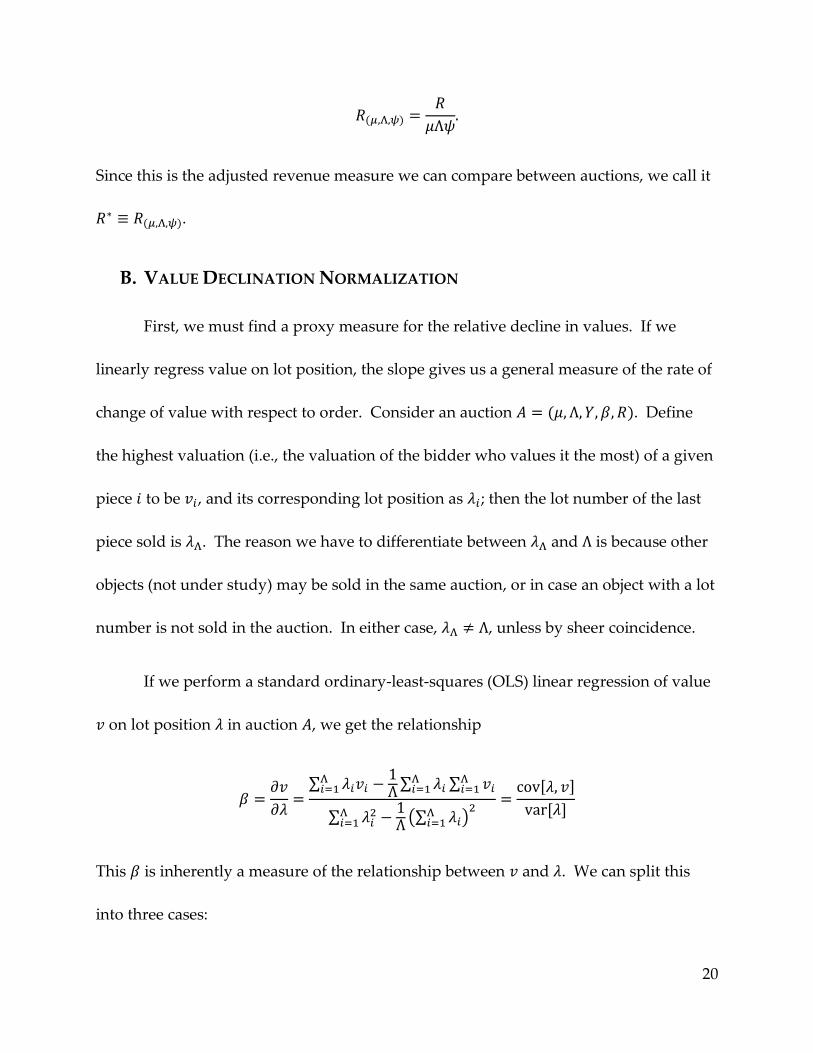
Since this is the adjusted revenue measure we can compare between auctions, we call it

.

B. VALUE DECLINATION NORMALIZATION

First, we must find a proxy measure for the relative decline in values. If we

linearly regress value on lot position, the slope gives us a general measure of the rate of

change of value with respect to order. Consider an auction . Define

the highest valuation (i.e., the valuation of the bidder who values it the most) of a given

piece to be , and its corresponding lot position as ; then the lot number of the last

piece sold is . The reason we have to differentiate between and is because other

objects (not under study) may be sold in the same auction, or in case an object with a lot

number is not sold in the auction. In either case, , unless by sheer coincidence.

If we perform a standard ordinary-least-squares (OLS) linear regression of value

on lot position in auction , we get the relationship

∑

∑

∑

∑

(∑

)

[ ]

[ ]

This is inherently a measure of the relationship between and . We can split this

into three cases:

21

(1) values decline over the course of the auction;

(2) values increase over the course of the auction;

(3) there is no general trend in the values over the course of the

auction.

From the magnitude of , we can gather the rate at which this decline/increase is

occurring. If and | | | |, then we can infer that the objects in were

organized more coherently in a declining order, i.e. the distribution of values is closer to

monotonic in lot order. Then, we expect that the effects of having declining values

should be stronger in than in .

Clearly, depends on several parameters within a given auction. These include

the lot position of the last object, the year in which the auction occurred, and the

characteristic value of the objects sold. These can be adjusted in the measurements we

use to calculate , namely and . We know

[ ]

[ ]

so if we normalize the lot numbers with respect to the last lot sold, we have a measure

that can be compared between auctions. Let’s call this measure . Then, we have

which gives us

22

[ ]

[ ]

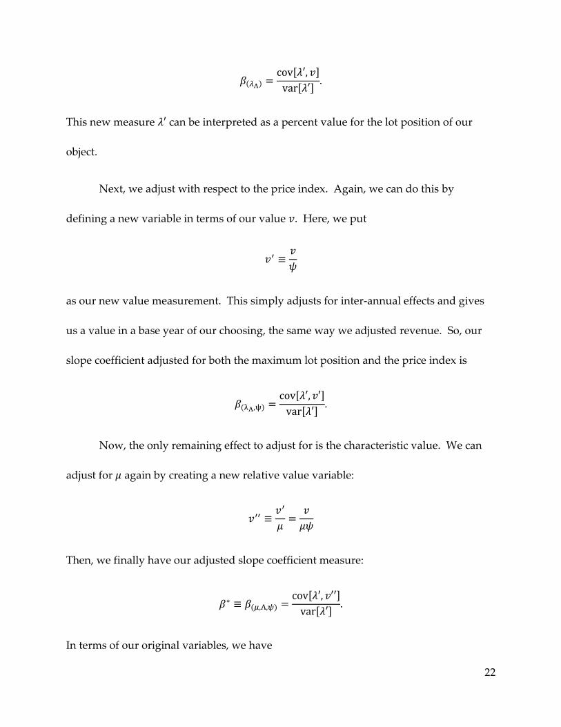
This new measure can be interpreted as a percent value for the lot position of our

object.

Next, we adjust with respect to the price index. Again, we can do this by

defining a new variable in terms of our value . Here, we put

as our new value measurement. This simply adjusts for inter-annual effects and gives

us a value in a base year of our choosing, the same way we adjusted revenue. So, our

slope coefficient adjusted for both the maximum lot position and the price index is

[ ]

[ ]

Now, the only remaining effect to adjust for is the characteristic value. We can

adjust for again by creating a new relative value variable:

Then, we finally have our adjusted slope coefficient measure:

[ ]

[ ]

In terms of our original variables, we have

23

[

]

[

]

[ ]

[ ]

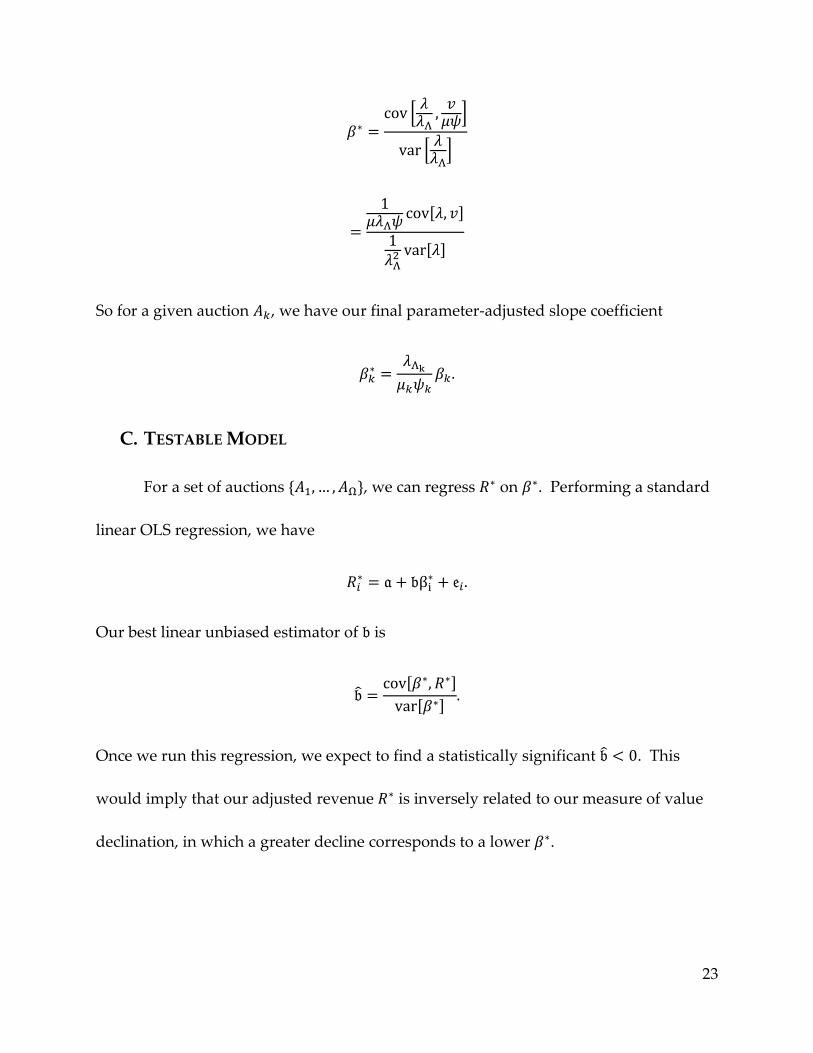
So for a given auction , we have our final parameter-adjusted slope coefficient

C. TESTABLE MODEL

For a set of auctions , we can regress on . Performing a standard

linear OLS regression, we have

Our best linear unbiased estimator of is

[ ]

[ ]

Once we run this regression, we expect to find a statistically significant . This

would imply that our adjusted revenue is inversely related to our measure of value

declination, in which a greater decline corresponds to a lower .

24

IV. DATA

This study uses two primary data sources, both of which I received through

contacts at the Duke Art, Law, and Markets Initiative (DALMI). For my Paris auction

data, I used a collection of auction records consolidated by Ms. Hilary Coe Smith, a PhD

candidate at Duke University’s Art, Art History, and Visual Studies department

(AAHVS). For the Christie’s auction data, I received permission from Christie’s

Archives to use a database compiled by Ms. Bénédicte Miyamoto-Pavot, a PhD

candidate at the Université Paris Diderot VII.

A. PARIS DATABASE

For my Paris auction data, I used Ms. Smith’s archives, which are now available

at Duke through the AAHVS server. These archives contain auction records from 1675

to 1814, and since I wanted to compare contemporary auctions, the first limiting factor

on my Paris dataset was the timeframe established by the Christie’s database (1767 to

1789). The second problem I faced was the lack of information on annual price levels in

Paris. I found two studies, but both stopped in 1786, so that became the second limiting

factor in which records I could use. The third issue was that the catalogs were not

organized by lot order, but by academic notions of prestige. For example, Italian

paintings were always placed first in the catalogs, regardless of the day of sale or the lot

number; these were followed by other schools of paintings (French, Spanish,

25

Dutch/Flemish, etc.), gouaches and miniatures, bronze and marble statues, designs,

prints, busts, and vases. Some catalogs, however, were accompanied by feuilles de

vacation (session sheets), which specified the day of sale and the lot position of each

piece. So, I restricted my study exclusively to those catalogs that included these

supplementary feuilles.

I did not have access to a database of these records. Instead, Ms. Smith had

collected images of individual pages from auction catalogs. She had not yet begun

transcribing the data for the time horizon that interested me, so a significant portion of

my background research involved recording the information from these catalogs in a

usable spreadsheet (see Appendix A). Each datum I logged had the following entries:

auction, day of sale, year of auction, lot position, catalog number, and sale price (in

livres, sous, and deniers). I then converted the sale price to a decimalized value

(denominated in livres), and adjusted these values for inflation using 1767 as my base

year.

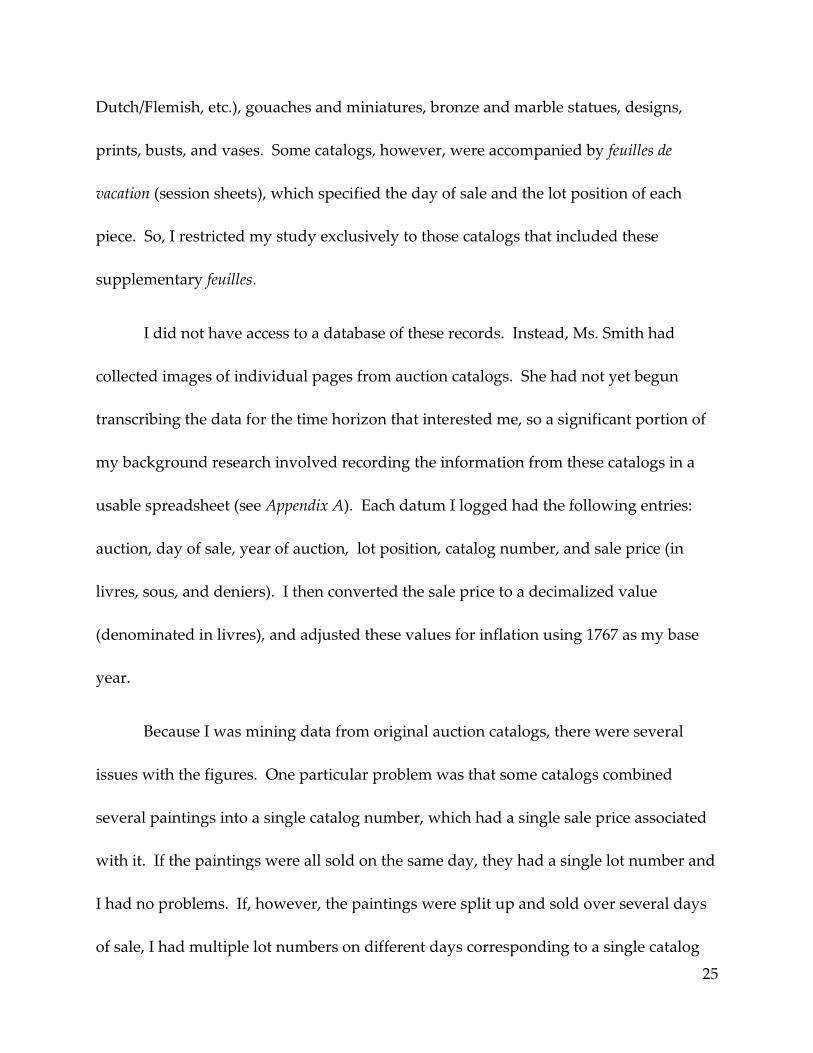
Because I was mining data from original auction catalogs, there were several

issues with the figures. One particular problem was that some catalogs combined

several paintings into a single catalog number, which had a single sale price associated

with it. If the paintings were all sold on the same day, they had a single lot number and

I had no problems. If, however, the paintings were split up and sold over several days

of sale, I had multiple lot numbers on different days corresponding to a single catalog

26

number, and hence one total price. In this case, since the paintings were grouped

because they were often identical, or at least very similar, I assumed that on average the

paintings sold for about the same price each day and divided the total sale price by the

number of days over which the catalog entry was sold. Another issue was that the

prices listed in the catalogs were handwritten by auction attendees. I had no way of

double-checking these sale prices, and I had to assume that the recorded sale prices

were correct. Since the sale prices are dependent variables in my model, I can assume

that any recording error was random, and thus my findings remain unbiased from this

error under Gauss-Markov assumptions (Wooldridge, 2009, p. 316). Again, since these

records were kept by audience members present at the auction, I also had to assume

that if a catalog entry had no sale price next to it, the piece was retired and not sold. In

the end, my Paris database comprised information on the sales of 1,485 paintings over

98 days of sale from 1767 to 1779.

Table 1: Paris Data Summary

Number of Auctions 98

Number of Lots 1484

Average Lots per Auction 15.143

Table 2: Paris Revenues Summary

Max 75% Median 25% Min IQR

68096.740 27191.486 15089.212 6450.532 73.812 20740.955

27

(N.B. Because lot values vary widely within a given auction, I used median statistics

rather than mean statistics to modulate the effects of tail behavior; see V. Results)

B. CHRISTIE’S DATABASE

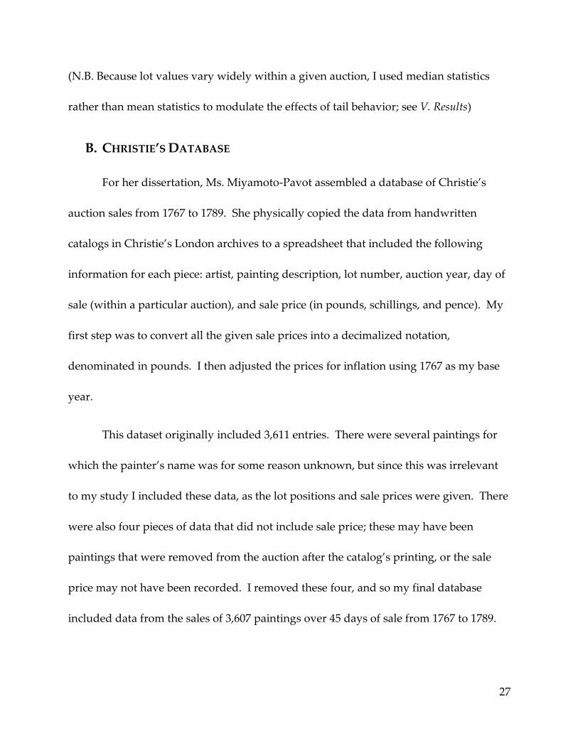
For her dissertation, Ms. Miyamoto-Pavot assembled a database of Christie’s

auction sales from 1767 to 1789. She physically copied the data from handwritten

catalogs in Christie’s London archives to a spreadsheet that included the following

information for each piece: artist, painting description, lot number, auction year, day of

sale (within a particular auction), and sale price (in pounds, schillings, and pence). My

first step was to convert all the given sale prices into a decimalized notation,

denominated in pounds. I then adjusted the prices for inflation using 1767 as my base

year.

This dataset originally included 3,611 entries. There were several paintings for

which the painter’s name was for some reason unknown, but since this was irrelevant

to my study I included these data, as the lot positions and sale prices were given. There

were also four pieces of data that did not include sale price; these may have been

paintings that were removed from the auction after the catalog’s printing, or the sale

price may not have been recorded. I removed these four, and so my final database

included data from the sales of 3,607 paintings over 45 days of sale from 1767 to 1789.

28

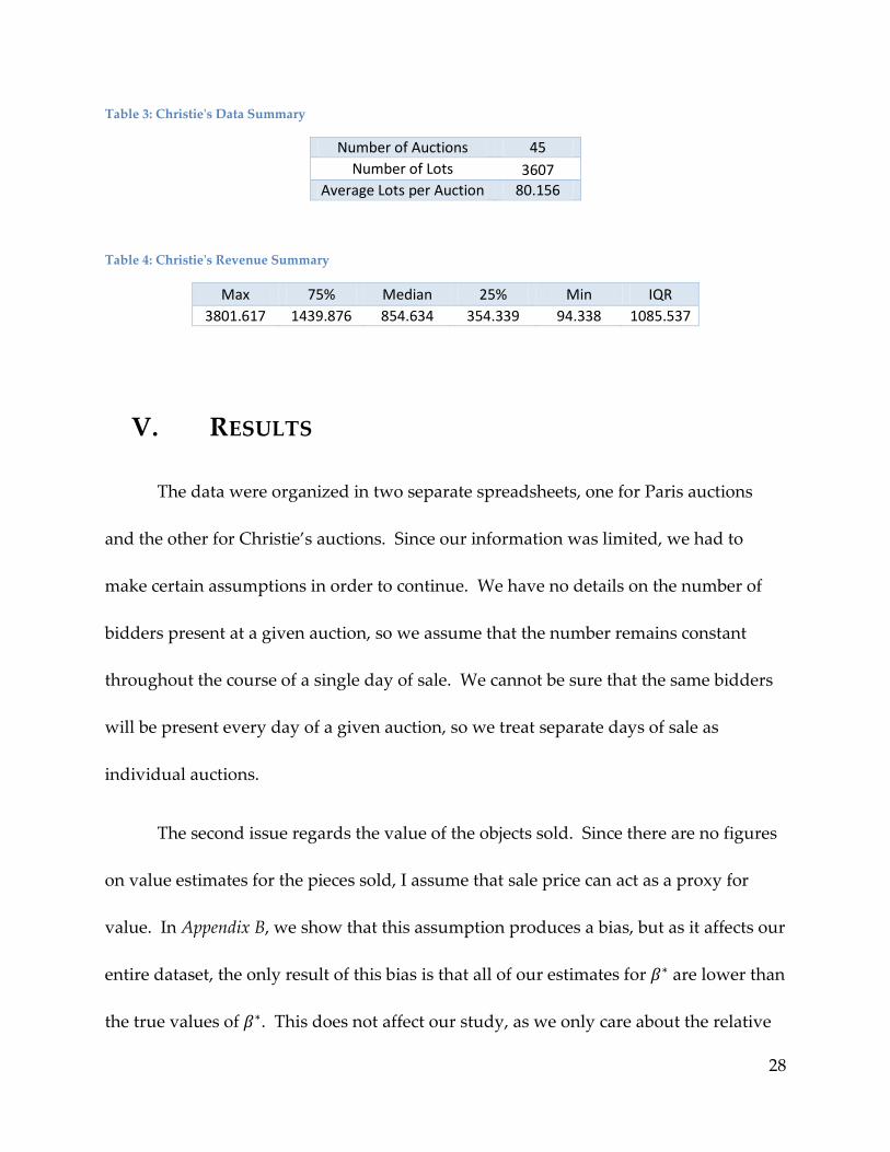
Table 3: Christie's Data Summary

Number of Auctions 45

Number of Lots 3607

Average Lots per Auction 80.156

Table 4: Christie's Revenue Summary

Max 75% Median 25% Min IQR

3801.617 1439.876 854.634 354.339 94.338 1085.537

V. RESULTS

The data were organized in two separate spreadsheets, one for Paris auctions

and the other for Christie’s auctions. Since our information was limited, we had to

make certain assumptions in order to continue. We have no details on the number of

bidders present at a given auction, so we assume that the number remains constant

throughout the course of a single day of sale. We cannot be sure that the same bidders

will be present every day of a given auction, so we treat separate days of sale as

individual auctions.

The second issue regards the value of the objects sold. Since there are no figures

on value estimates for the pieces sold, I assume that sale price can act as a proxy for

value. In Appendix B, we show that this assumption produces a bias, but as it affects our

entire dataset, the only result of this bias is that all of our estimates for are lower than

the true values of . This does not affect our study, as we only care about the relative

29

differentiation between values of , not the specific values themselves. This bias will

further cause our estimate of to be lower than the true value, but again all we are

looking for is the sign of , so it is irrelevant to our study. So although the bias exists, it

does not alter the findings.

The third thing we must consider is the characteristic value. Since art prices tend

to have extreme right-tail events, skewing the distribution, the mean is not an accurate

indicator of the average. We want to reduce the effects of tail events, and the median

provides a more robust estimator of location than the mean. So, we set to be the

median sale price in a given auction. Since the standard deviation is a measure of

variability corresponding to the mean, we use the interquartile range defined as

, or the range of the middle of values, as our robust measure of

statistical dispersion rather than the standard deviation. is analogous to for a

distribution determined by mean and variance, .

A. PARIS RESULTS

From our Paris data, we have the following summary statistics:

Table 5: Paris R* and β* Statistics

Min 25% Median 75% Max IQR

R* 0.669 1.198 1.585 2.491 11.153 1.293

β* -37.943 -1.790 -0.260 0.946 5.716 2.736

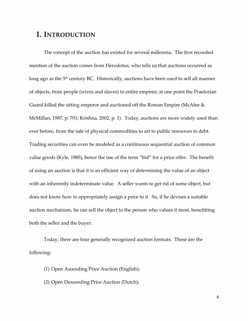
We run the following OLS regression of on :

30

This gives us the following results:

Table 6: Paris Coefficient Estimates

Coefficient Estimate Std Error t Ratio Prob > |t|

a 1.171 0.111 10.51 <.0001

b -0.312 0.017 -18.47 <.0001

So we have the following regression:

Figure 1: Paris Auctions – R* vs. β*

-2

0

2

4

6

8

10

12

14

-40 -35 -30 -25 -20 -15 -10 -5 0 5

R*

β*

Paris Auctions - R* vs. β*

31

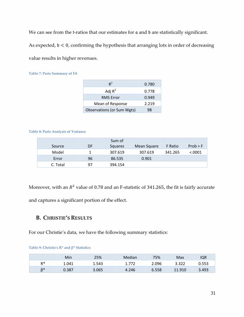
We can see from the t-ratios that our estimates for and are statistically significant.

As expected, , confirming the hypothesis that arranging lots in order of decreasing

value results in higher revenues.

Table 7: Paris Summary of Fit

R2 0.780

Adj R2 0.778

RMS Error 0.949

Mean of Response 2.219

Observations (or Sum Wgts) 98

Table 8: Paris Analysis of Variance

Source DF Sum of Squares Mean Square F Ratio Prob > F

Model 1 307.619 307.619 341.265 <.0001

Error 96 86.535 0.901 C. Total 97 394.154

Moreover, with an value of and an F-statistic of , the fit is fairly accurate

and captures a significant portion of the effect.

B. CHRISTIE’S RESULTS

For our Christie’s data, we have the following summary statistics:

Table 9: Christie's R* and β* Statistics

Min 25% Median 75% Max IQR

R* 1.041 1.543 1.772 2.096 3.322 0.553

β* 0.387 3.065 4.246 6.558 11.910 3.493

32

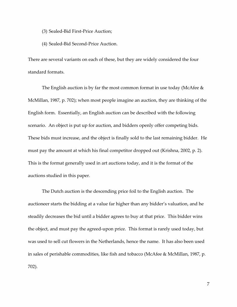
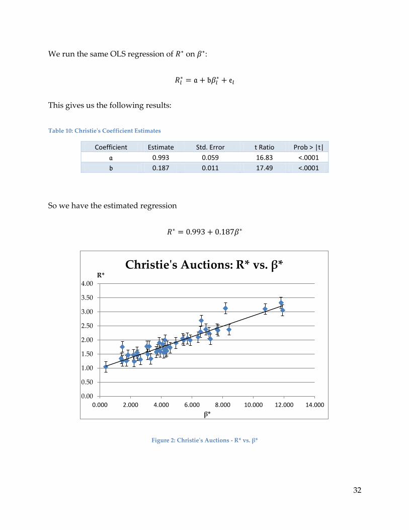
We run the same OLS regression of on :

This gives us the following results:

Table 10: Christie's Coefficient Estimates

Coefficient Estimate Std. Error t Ratio Prob > |t|

a 0.993 0.059 16.83 <.0001

b 0.187 0.011 17.49 <.0001

So we have the estimated regression

Figure 2: Christie's Auctions - R* vs. β*

0.00

0.50

1.00

1.50

2.00

2.50

3.00

3.50

4.00

0.000 2.000 4.000 6.000 8.000 10.000 12.000 14.000

R*

β*

Christie's Auctions: R* vs. β*

33

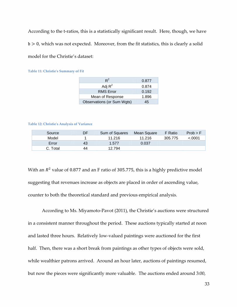
According to the t-ratios, this is a statistically significant result. Here, though, we have

, which was not expected. Moreover, from the fit statistics, this is clearly a solid

model for the Christie’s dataset:

Table 11: Christie's Summary of Fit

R2 0.877

Adj R2 0.874

RMS Error 0.192

Mean of Response 1.896

Observations (or Sum Wgts) 45

Table 12: Christie's Analysis of Variance

Source DF Sum of Squares Mean Square F Ratio Prob > F

Model 1 11.216 11.216 305.775 <.0001

Error 43 1.577 0.037 C. Total 44 12.794

With an value of and an F ratio of , this is a highly predictive model

suggesting that revenues increase as objects are placed in order of ascending value,

counter to both the theoretical standard and previous empirical analysis.

According to Ms. Miyamoto-Pavot (2011), the Christie’s auctions were structured

in a consistent manner throughout the period. These auctions typically started at noon

and lasted three hours. Relatively low-valued paintings were auctioned for the first

half. Then, there was a short break from paintings as other types of objects were sold,

while wealthier patrons arrived. Around an hour later, auctions of paintings resumed,

but now the pieces were significantly more valuable. The auctions ended around 3:00,

34

after which dinner was served. This was the standard format for auctions in 18th

century London. It may make sense, then, that if such a pattern were institutional,

bidders would adjust their strategies to account for the change in the value of the

paintings from the first part of the auction to the second part.

In Appendix C, we run a simple test to see if there was a specific pattern followed

in the ordering of lots at Christie’s auctions compared to those in Paris. Based on the

analysis, there was considerable variability in the value-ordering at the Paris auctions,

and relatively little variation in the pattern at Christie’s. This implies that there was in

fact a very regular process at Christie’s, and bidders could adjust their strategies to

account for this, explaining the discrepancy in our results for the Christie’s data.

VI. CONCLUSIONS

Using our data from Paris auctions, we find that the model developed in this

paper supports the claim that ordering lots in decreasing value generates higher

revenues for the seller. The data from Christie’s does not support the hypothesis, but as

demonstrated in Appendix C, this is due to structural praxes stemming from an

institutionally regular pattern at Christie’s during this period.

35

For our set of Paris auctions, we find that the relationship between the adjusted

revenue and the adjusted slope coefficient is proportional (disregarding the constant)

with a factor of , and this measure has a t-statistic of , so it is a

statistically significant relationship.

Modern empirical studies generally focus on recent auctions that have occurred

since the theory was developed, and until now nobody has studied historical auctions.

This study provides some evidence that this optimal ordering is not related to modern

practices by auction houses. There is, however, definite need to expand this study.

There remains a substantial supply of unexamined auction records from Paris, available

through the AAHVS server at Duke. This study meant to compare the information

about contemporary Paris and Christie’s auctions, but a new study could focus solely

on Paris auctions over centuries, providing further insights into our assumed optimality

conditions for sequential auctions. Another study could consider variations on the

basic model outlined here, either by incorporating more details about individual pieces

of art or the auctions themselves. A further extension could consider using a modified

characteristic value,

, for each auction, using an analog of the Sharpe ratio for

median statistics.

36

REFERENCES

Ashenfelter, O. (1989). How Auctions Work for Wine and Art. The Journal of Economic

Perspectives, 23-36.

Ashenfelter, O., & Genesove, D. (1992). Testing for Price Anomalies in Real-Estate

Auctions. The American Economic Review, 501-505.

Ashenfelter, O., & Graddy, K. (2003). Auctions and the Price of Art. Journal of Economic

Literature, 763-787.

Ausubel, L. (1997). On Generalizing the English Auction. 1-14.

Beggs, A., & Graddy, K. (1997). Declining Values and the Afternoon Effect: Evidence

from Art Auctions. The RAND Journal of Economics, 544-565.

Benoit, J.-P., & Krishna, V. (2001). Multiple-Object Auctions with Budget Constrained

Bidders. Review of Economic Studies, 155-179.

Birulin, O., & Izmalkovy, S. (2009). On Efficiency of the English Auction. CEFIR/NES

Working Paper Series, 1-28.

Elkind, E., & Fatima, S. (2007). Maximizing Revenue in Sequential Auctions. WINE, 491-

502.

Elmaghraby, W. (2003). The Importance of Ordering in Sequential Auctions.

Management Science, 673-682.

37

Ginsburgh, V. (1998). Bidders and the Declining Price Anomaly in Wine Auctions.

Journal of Political Economy, 1302-1319.

Goncalves, R. (2008). Irrationality in English Auctions. Journal of Economic Behavior &

Organization, 180-192.

Hong, H., Kremer, I., Kubik, J., Mei, J., & Moses, M. (2009). Who's on First? Ordering

and Revenue in Art Auctions. 1-41.

Kagel, J. H., & Levin, D. (1993). Independent Private Value Auctions: Bidder Behaviour

in First-, Second- and Third-Price Auctions with Varying Numbers of Bidders.

The Economic Journal, 868-879.

Krishna, V. (2002). Auction Theory. San Diego: Elsevier Science.

Kyle, A. S. (1985). Continuous Auctions and Insider Trading. Econometrica, 1315-1335.

Li, H., & Riley, J. G. (2007). Auction Choice. International Journal of Industrial

Organization, 1269-1298.

Maskin, E., & Riley, J. (2000). Equilibrium in Sealed High Bid Auctions. Review of

Economic Studies, 439-454.

McAfee, R. P., & McMillan, J. (1987). Auctions and Bidding. Journal of Economic

Literature, 699-738.

38

McAfee, R. P., & Vincent, D. (1993). The Declining Price Anomaly. Journal of Economic

Theory, 191-212.

Milgrom, P. R., & Weber, R. J. (1982). A Theory of Auctions and Competitive Bidding.

Econometrica, 1089-1122.

Milgrom, P., & Weber, R. J. (1982). The Value of Information in a Sealed-Bid Auction.

Journal of Mathematical Economics, 105-114.

Miyamoto-Pavot, B. (2011, November 2). Christie's 18th Century Auctions. (A. Mitha,

Interviewer)

Myerson, R. B. (1981). Optimal Auction Design. Mathematics of Operations Research, 58-

73.

Neeman, Z. (2003). The Effectiveness of English Auctions. Games and Economic Behavior,

214-238.

Pitchik, C. (2006). Budget-Constrained Sequential Auctions with Incomplete

Information. 1-35.

Riley, J. G., & Samuelson, W. F. (1981). Optimal Auctions. The American Economic Review,

381-392.

Twigger, R. (1999). Inflation: the Value of the Pound 1750-1998. House of Commons

Library, 1-20.

39

Vickrey, W. (1961). Counterspeculation, Auctions, and Competitive Sealed Tenders. The

Journal of Finance, 8-37.

Wooldrige, J. M. (2009). Introductory Econometrics: A Modern Approach. Mason, OH:

South-Western Cengage Learning.

Zulehner, C. (2009). Bidding Behavior in Sequential Cattle Auctions. International Journal

of Industrial Organization, 33-42.

40

APPENDICES

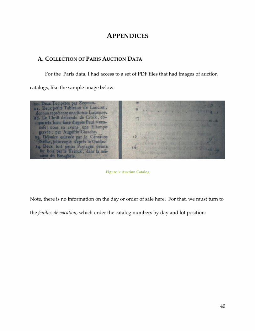
A. COLLECTION OF PARIS AUCTION DATA

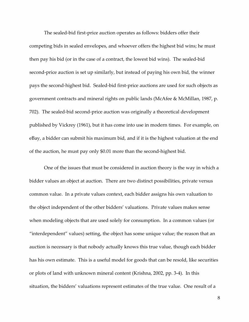
For the Paris data, I had access to a set of PDF files that had images of auction

catalogs, like the sample image below:

Figure 3: Auction Catalog

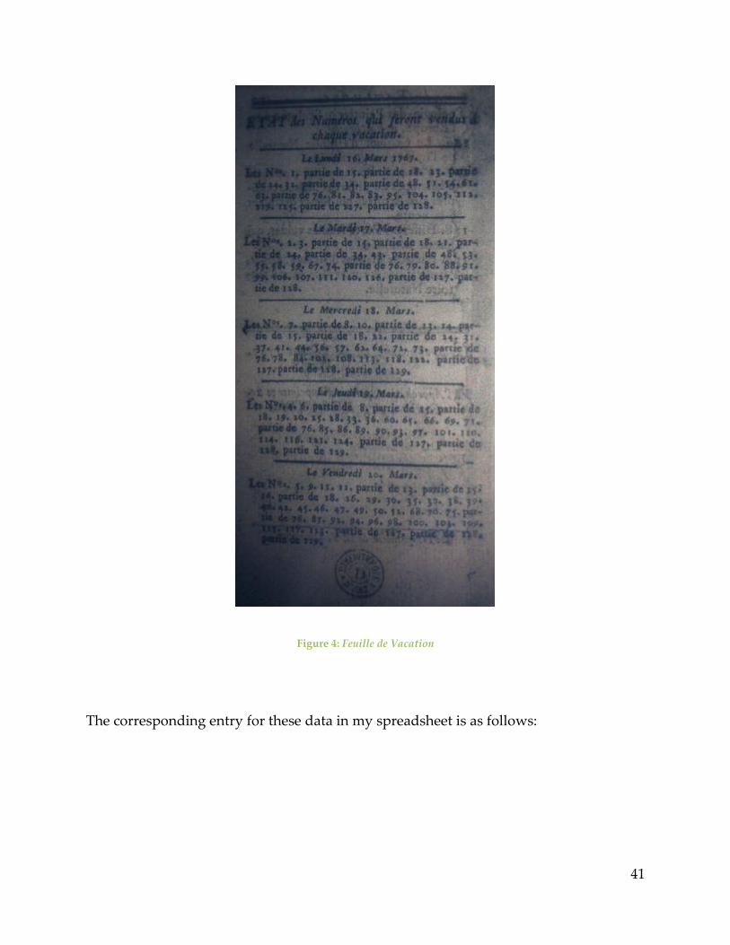
Note, there is no information on the day or order of sale here. For that, we must turn to

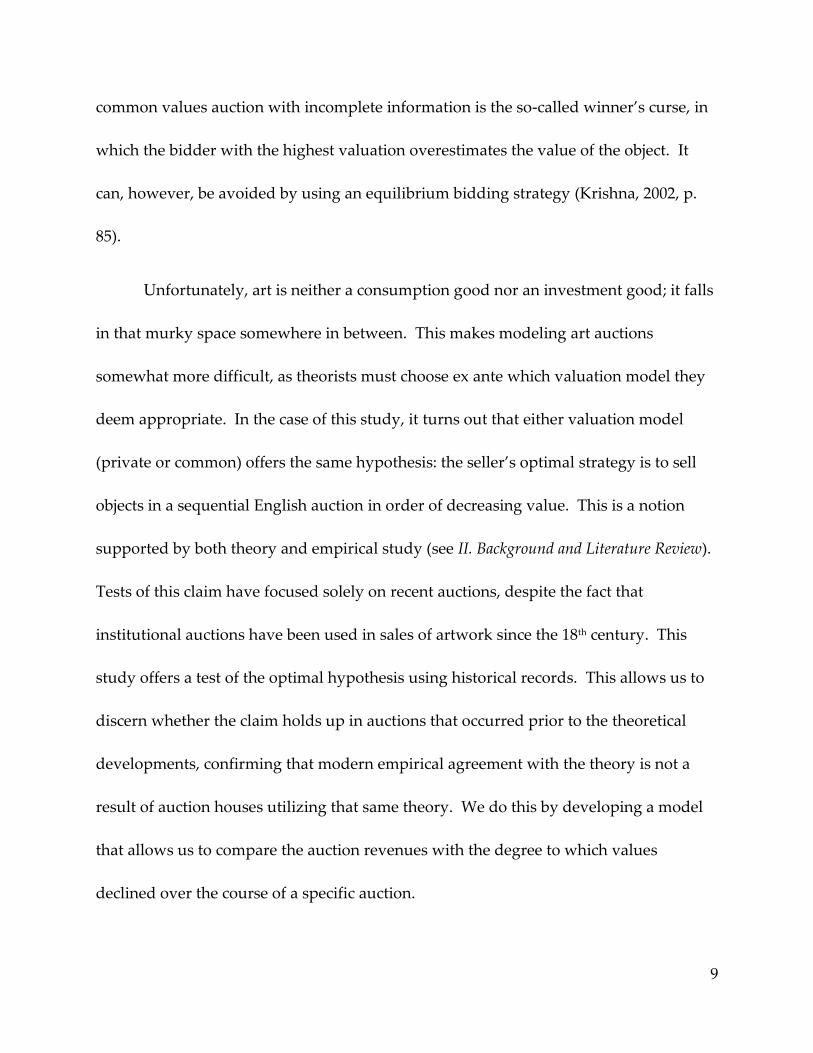
the feuilles de vacation, which order the catalog numbers by day and lot position:

41

Figure 4: Feuille de Vacation

The corresponding entry for these data in my spreadsheet is as follows:

42

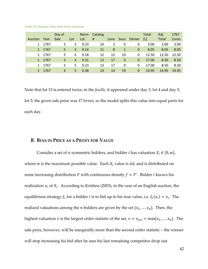
Table 13: Sample Data from Paris Auctions

Auction Year Day of Sale Lot

Norm Lot

Catalog # Livre Sous Denier

Total (L)

Adj Total

1767 Livres

1 1767 3 3 0.23 10 3 0 0 3.00 3.00 3.00

1 1767 5 3 0.14 11 8 1 0 8.05 8.05 8.05

1 1767 5 4 0.18 12 12 10 0 12.50 12.50 12.50

1 1767 3 4 0.31 13 17 0 0 17.00 8.50 8.50

1 1767 5 5 0.23 13 17 0 0 17.00 8.50 8.50

1 1767 3 5 0.38 14 14 19 0 14.95 14.95 14.95

Note that lot 13 is entered twice; in the feuille, it appeared under day 3, lot 4 and day 5,

lot 5; the given sale price was 17 livres, so the model splits this value into equal parts for

each day.

B. BIAS IN PRICE AS A PROXY FOR VALUE

Consider a set of symmetric bidders, and bidder has valuation [ ],

where is the maximum possible value. Each value is iid, and is distributed on

some increasing distribution with continuous density . Bidder knows his

realization of . According to Krishna (2003), in the case of an English auction, the

equilibrium strategy for a bidder is to bid up to his true value, i.e. . The

realized valuations among the bidders are given by the set . Then, the

highest valuation is the largest order statistic of the set, . The

sale price, however, will be marginally more than the second order statistic – the winner

will stop increasing his bid after he sees his last remaining competitor drop out.

43

Without loss of generality, assume , and . If

, we have the sale price . Otherwise, in the marginal unit. If

, we again have . Otherwise, , so . Therefore, we must

have the relationship , and the winning bidder must have a nonnegative surplus,

i.e. .

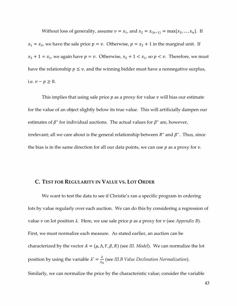
This implies that using sale price as a proxy for value will bias our estimate

for the value of an object slightly below its true value. This will artificially dampen our

estimates of for individual auctions. The actual values for are, however,

irrelevant; all we care about is the general relationship between and . Thus, since

the bias is in the same direction for all our data points, we can use as a proxy for .

C. TEST FOR REGULARITY IN VALUE VS. LOT ORDER

We want to test the data to see if Christie’s ran a specific program in ordering

lots by value regularly over each auction. We can do this by considering a regression of

value on lot position . Here, we use sale price as a proxy for (see Appendix B).

First, we must normalize each measure. As stated earlier, an auction can be

characterized by the vector (see III. Model). We can normalize the lot

position by using the variable

(see III.B Value Declination Normalization).

Similarly, we can normalize the price by the characteristic value; consider the variable

44

. This is analogous to our original adjustment of the revenue by the characteristic

value, where we found

(see III.A Revenue Normalization). Clearly, revenue is the

sum of the prices in an auction, so ∑ . It follows that

∑

∑

∑

so our price transformation

preserves our original revenue transformation.

Now, since we want to look at the trends with respect to the lot position, we’ll

study the relative values for each decile of the normalized lot variable. For the Paris

data, we have the following statistics:

Table 14: Aggregate Paris Decile Statistics

Decile Q3 Q1 Q2 QCoD CV

1 0.963 0.095 0.265 0.820 163.5%

2 1.579 0.141 0.420 0.836 171.1%

3 1.160 0.029 0.257 0.951 220.4%

4 2.393 0.148 0.485 0.884 231.5%

5 4.738 0.300 0.739 0.881 300.2%

6 2.181 0.225 0.746 0.813 131.1%

7 2.396 0.161 0.677 0.874 165.0%

8 1.918 0.154 0.503 0.851 175.4%

9 2.139 0.118 0.544 0.895 185.7%

10 0.814 0.029 0.191 0.932 206.1%

Again, since our distribution is skewed, we want a measure that does not heavily

weigh outliers, so we use quartile statistics. Here, the deciles each represent one-tenth

of the lots, i.e. the first decile corresponds to the interval ], the second decile

45

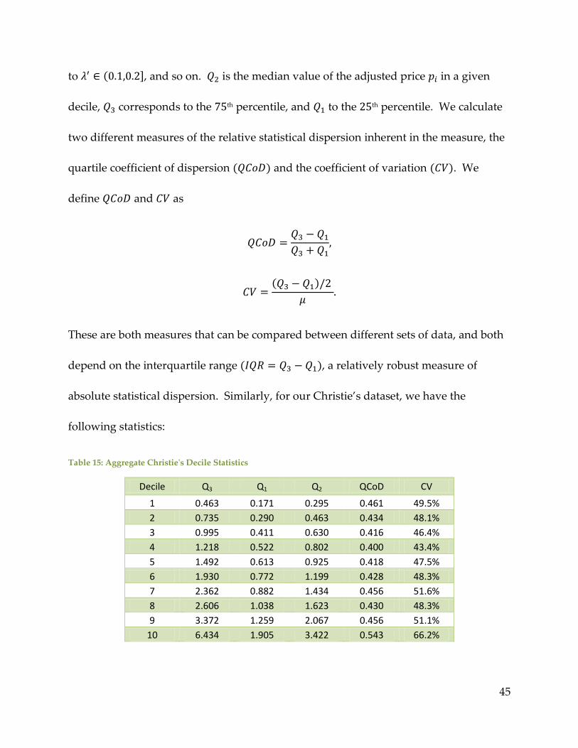
to ], and so on. is the median value of the adjusted price in a given

decile, corresponds to the th percentile, and to the th percentile. We calculate

two different measures of the relative statistical dispersion inherent in the measure, the

quartile coefficient of dispersion and the coefficient of variation . We

define and as

These are both measures that can be compared between different sets of data, and both

depend on the interquartile range , a relatively robust measure of

absolute statistical dispersion. Similarly, for our Christie’s dataset, we have the

following statistics:

Table 15: Aggregate Christie's Decile Statistics

Decile Q3 Q1 Q2 QCoD CV

1 0.463 0.171 0.295 0.461 49.5%

2 0.735 0.290 0.463 0.434 48.1%

3 0.995 0.411 0.630 0.416 46.4%

4 1.218 0.522 0.802 0.400 43.4%

5 1.492 0.613 0.925 0.418 47.5%

6 1.930 0.772 1.199 0.428 48.3%

7 2.362 0.882 1.434 0.456 51.6%

8 2.606 1.038 1.623 0.430 48.3%

9 3.372 1.259 2.067 0.456 51.1%

10 6.434 1.905 3.422 0.543 66.2%

46

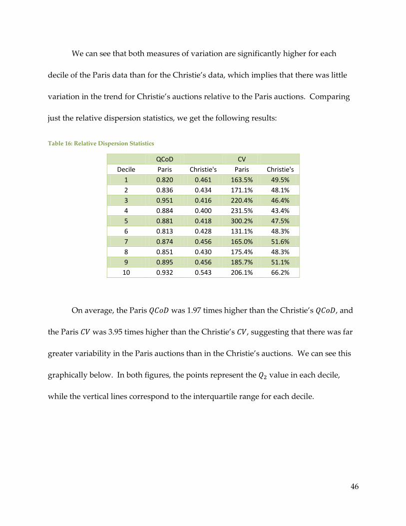
We can see that both measures of variation are significantly higher for each

decile of the Paris data than for the Christie’s data, which implies that there was little

variation in the trend for Christie’s auctions relative to the Paris auctions. Comparing

just the relative dispersion statistics, we get the following results:

Table 16: Relative Dispersion Statistics

QCoD

CV

Decile Paris Christie's Paris Christie's

1 0.820 0.461 163.5% 49.5%

2 0.836 0.434 171.1% 48.1%

3 0.951 0.416 220.4% 46.4%

4 0.884 0.400 231.5% 43.4%

5 0.881 0.418 300.2% 47.5%

6 0.813 0.428 131.1% 48.3%

7 0.874 0.456 165.0% 51.6%

8 0.851 0.430 175.4% 48.3%

9 0.895 0.456 185.7% 51.1%

10 0.932 0.543 206.1% 66.2%

On average, the Paris was 1.97 times higher than the Christie’s , and

the Paris was 3.95 times higher than the Christie’s , suggesting that there was far

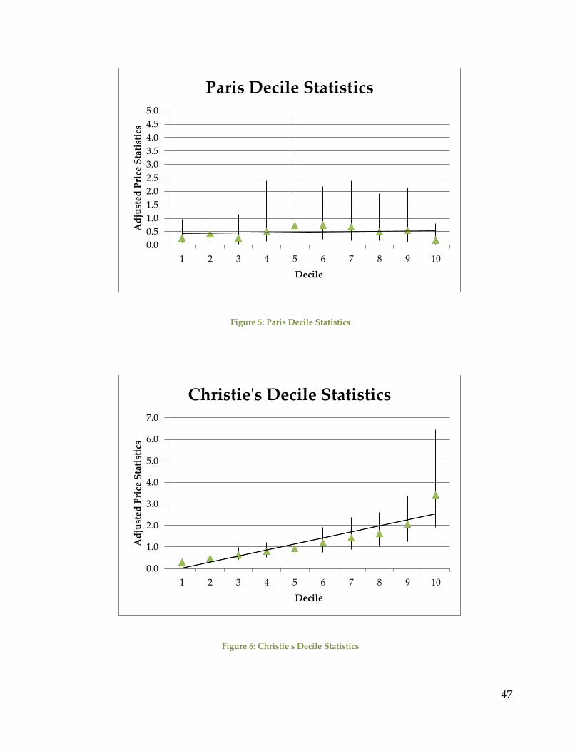
greater variability in the Paris auctions than in the Christie’s auctions. We can see this

graphically below. In both figures, the points represent the value in each decile,

while the vertical lines correspond to the interquartile range for each decile.

47

Figure 5: Paris Decile Statistics

Figure 6: Christie's Decile Statistics

0.0

0.5

1.0

1.5

2.0

2.5

3.0

3.5

4.0

4.5

5.0

1 2 3 4 5 6 7 8 9 10

Ad

just

ed P

rice

Sta

tist

ics

Decile

Paris Decile Statistics

0.0

1.0

2.0

3.0

4.0

5.0

6.0

7.0

1 2 3 4 5 6 7 8 9 10

Ad

just

ed P

rice

Sta

tist

ics

Decile

Christie's Decile Statistics

48

We can see that the Christie’s distribution fits the description provided by Ms.

Miyamoto-Pavot, with a general upward trend in value as the relative lot number

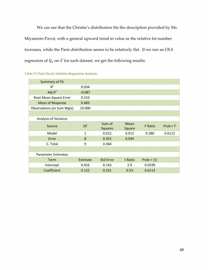
increases, while the Paris distribution seems to be relatively flat. If we run an OLS

regression of on for each dataset, we get the following results:

Table 17: Paris Decile Statistics Regression Analysis

Summary of Fit

R2 0.034

Adj R2 -0.087

Root Mean Square Error 0.210

Mean of Response 0.483

Observations (or Sum Wgts) 10.000

Analysis of Variance

Source DF Sum of Squares

Mean Square

F Ratio Prob > F

Model 1 0.012 0.012 0.280 0.6113

Error 8 0.352 0.044

C. Total 9 0.364

Parameter Estimates

Term Estimate Std Error t Ratio Prob > |t|

Intercept 0.416 0.143 2.9 0.0199

Coefficient 0.122 0.231 0.53 0.6113

49

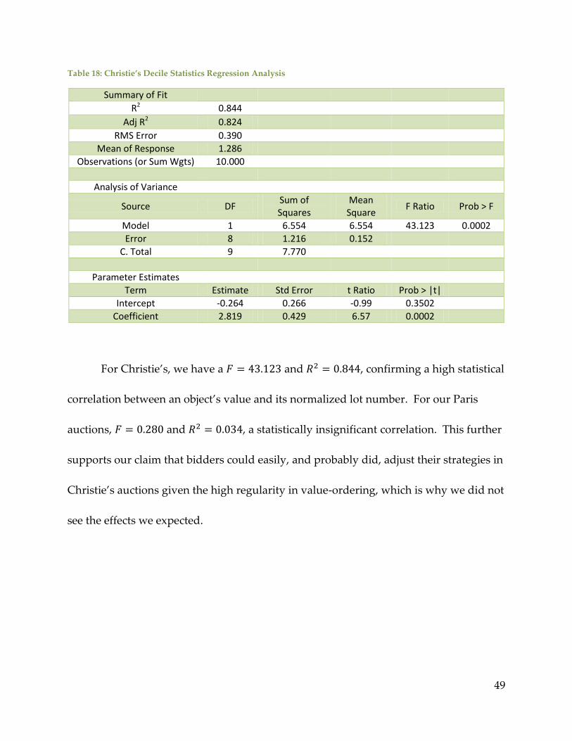
Table 18: Christie’s Decile Statistics Regression Analysis

Summary of Fit

R2 0.844

Adj R2 0.824

RMS Error 0.390

Mean of Response 1.286

Observations (or Sum Wgts) 10.000

Analysis of Variance

Source DF Sum of Squares

Mean Square

F Ratio Prob > F

Model 1 6.554 6.554 43.123 0.0002

Error 8 1.216 0.152

C. Total 9 7.770

Parameter Estimates

Term Estimate Std Error t Ratio Prob > |t|

Intercept -0.264 0.266 -0.99 0.3502

Coefficient 2.819 0.429 6.57 0.0002

For Christie’s, we have a and , confirming a high statistical

correlation between an object’s value and its normalized lot number. For our Paris

auctions, and , a statistically insignificant correlation. This further

supports our claim that bidders could easily, and probably did, adjust their strategies in

Christie’s auctions given the high regularity in value-ordering, which is why we did not

see the effects we expected.