Ordinal Arithmetic: Algorithms and Mechanization

Panagiotis Manolios (manolios@cc.gatech.edu)College of Computing, CERCS Lab, Georgia Institute of Technology801 Atlantic Drive, Atlanta, Georgia 30332-0280 U.S.A.http://www.cc.gatech.edu/∼manolios

Daron Vroon (vroon@cc.gatech.edu)College of Computing, CERCS Lab, Georgia Institute of Technology801 Atlantic Drive, Atlanta, Georgia 30332-0280 U.S.A.http://www.cc.gatech.edu/∼vroon

Abstract. Termination proofs are of critical importance for establishing the cor-rect behavior of both transformational and reactive computing systems. A generalsetting for establishing termination proofs involves the use of the ordinal numbers,an extension of the natural numbers into the transfinite which were introduced byCantor in the nineteenth century and are at the core of modern set theory. Wepresent the first comprehensive treatment of ordinal arithmetic on compact ordinalnotations and give efficient algorithms for various operations, including addition,subtraction, multiplication, and exponentiation.

Using the ACL2 theorem proving system, we implemented our ordinal arithmeticalgorithms, mechanically verified their correctness, and developed a library of theo-rems that can be used to significantly automate reasoning involving the ordinals. Toenable users of the ACL2 system to fully utilize our work required that we modifyACL2, e.g., we replaced the underlying representation of the ordinals and added alarge library of definitions and theorems. Our modifications are available startingwith ACL2 version 2.8.

1. Introduction

Termination proofs are of critical importance for mechanically estab-lishing that computing systems behave correctly. In the case of trans-formational systems, termination proofs allow us to go from partialcorrectness to total correctness [1]. Termination proofs are importanteven in the context of reactive systems, non-terminating systems thatare engaged in on-going interaction with an environment (e.g., net-work protocols, operating systems, distributed databases, pipelinedmachines, etc.): they are used to prove liveness properties i.e., to showthat some desirable behavior is not postponed forever. Proving ter-mination amounts to showing that a relation is well-founded [2]. Anywell-founded relation can be extended to a total order, giving rise toa well-ordered relation. From a basic theorem of set theory, we havethat every well-ordered relation is isomorphic to an ordinal; thus, the

c© 2005 Kluwer Academic Publishers. Printed in the Netherlands.

ordinals.tex; 16/03/2005; 12:41; p.1

2

ordinal numbers provide a general setting for establishing terminationproofs.

1.1. Previous Work

The ordinal numbers were introduced by Cantor over 100 years ago andare at the core of modern set theory [10, 11, 12]. They are an extensionof the natural numbers into the transfinite and are an important tool inlogic, e.g., after Gentzen’s proof of the consistency of Peano arithmeticusing the ordinal number ε0 [21], proof theorists routinely use ordinalsand ordinal notations to establish the consistency of logical theories [57,62]. To obtain constructive proofs, constructive ordinals notations areemployed. The general theory of ordinal notations was initiated byChurch and Kleene [13] and is recounted in Chapter 11 of Roger’sbook on computability [50].

An early use of the ordinals for proving program termination is dueto Alan M. Turing, who in 1949 wrote the following [64, 42].

The checker has to verify that the process comes to an end. Hereagain he should be assisted by the programmer giving a furtherdefinite assertion to be verified. This may take the form of a quan-tity which is asserted to decrease continually and vanish when themachine stops. To the pure mathematician it is natural to give anordinal number. In this problem the ordinal might be (n − r)ω2 +(r − s)ω + k.1

The automated reasoning community has studied the problem offormalizing the ordinals (as opposed to ordinal notations), focusing onproving known results. Dennis and Smaill studied higher-order heuristicextensions of rippling. They used ordinal arithmetic as a case study,which was implemented in λClam, a higher order proof planning sys-tem for induction. They were able to successfully plan standard un-dergraduate textbook problems using their system [14]. Paulson andGrabczewski have mechanized a good deal of set theory, including theproof that for any infinite cardinal, κ, we have κ ⊗ κ = κ, most of thefirst chapter of Kunen’s excellent book on set theory [30], and the equiv-alence of eight forms of the well-ordering theorem [49]. More recently,Paulson has mechanized the proof of the relative consistency of theaxiom of choice and has proved the reflection theorem [48, 47]. Paulsonand Grabczewski’s efforts required reasoning about the ordinals and

1 Readers familiar with the ordinals may suspect that Turing’s measure functionis not quite right, as (i)ωj = ωj when i and j are positive integers. This seems to bepurely a notational issue, e.g., Turing uses the same convention in a paper on logicsbased on ordinals [63]. Using modern conventions, the measure function is writtenω2(n − r) + ω(r − s) + k.

ordinals.tex; 16/03/2005; 12:41; p.2

Ordinal Arithmetic: Algorithms and Mechanization 3

were carried out with the Isabelle/ZF system [44, 46]. A version ofthe reflection theorem was also proved by Bancerek, using Mizar [3].Another line of work is by Belinfante, who has used Otter to proveelementary theorems of ordinal number theory [4, 5, 6]. There is muchmore work that can be mentioned, but we end by listing some of thetheorem proving systems for which there exists support for the ordinals:Nqthm [8], ACL2 [26], Coq [7], PVS [43], HOL [22], Isabelle [45], andMizar [51].

Ordinal notations are used in the context of automated reasoningto prove termination. For example, the ordinals up to ε0 are the basisfor termination proofs in the ACL2 theorem proving system [26, 27],which has been used on some impressive industrial-scale problems bycompanies such as AMD, Rockwell Collins, Motorola, and IBM. ACL2was used to prove that the floating-point operations performed by AMDmicroprocessors are IEEE-754 compliant [41, 54], to analyze bit andcycle accurate models of the Motorola CAP, a digital signal processor[9], and to analyze a model of the JEM1, the world’s first silicon JVM(Java Virtual Machine) [24]. Termination proofs have played a key rolein various projects that use ACL2 to verify reactive systems. For exam-ple, in [32], we develop a theory of refinement for reactive systems thathas been used to mechanically verify protocols, pipelined machines,and distributed systems [35, 31, 60]. Ordinals have also played a keyrole in projects to implement polynomial orderings [39] and multisetrelations [52]. The relationship between proof theoretic ordinals andterm rewriting is explored in [15, 20].

1.2. The Ordinal Arithmetic Problem

Despite the fact that ordinals have been studied and used extensively byvarious communities for over 100 years, we have not been able to find acomprehensive treatment of arithmetic on ordinal notations. The ordi-nal arithmetic problem for a notational system denoting the ordinals upto some ordinal δ, is as follows: given α and β, expressions in the systemdenoting ordinals < δ, is γ the expression corresponding to α?β, where? can be any of +,−, ·, exponentiation? Solving this problem amountsto defining algorithms for ordinal arithmetic on the notation system inquestion. The practical implications of a solution to the ordinal arith-metic problem is that it allows users of theorem proving systems suchas ACL2 to think and reason about ordinals algebraically. Algebraicreasoning is more convenient and powerful than the previously availableoptions, which required users to use the underlying representation ofordinals to both define measure functions and to reason about them.

ordinals.tex; 16/03/2005; 12:41; p.3

4

In this paper, we present a solution to the ordinal arithmetic problemfor a notational system denoting the ordinals up to ε0. Partial solutionsto this problem appear in various books and papers [57, 16, 20, 40,58, 62], e.g., it is easy to find a definition of < for various ordinalnotations, but we have not found any statement of the problem norany comprehensive solution in previous work. One notable exceptionis the dissertation work of John Doner [19, 18]. Doner and Tarski (hisadviser) study hierarchies of ordinal arithmetic operations. They give atransfinite recursive definition for binary operations Oγ for any ordinalγ. The operation O0 corresponds to addition, O1 corresponds to mul-tiplication, O2 corresponds to exponentiation (for the most part), andso on. Using this hierarchy of operations, Doner and Tarski define ageneralization of the Cantor normal form. However, Doner and Tarskistop short of defining an ordinal notation. They give pseudo-algorithmsfor O1, O2, and O3, but it is not immediately clear how to apply these toan ordinal notation to obtain algorithms. This was not within the scopeof their work, as they were studying operations on the set-theoreticordinals, not on ordinal notations.

We use a notational system that is exponentially more succinct thanthe one used in ACL2 before version 2.8 and we give efficient algorithms,whose complexity we analyze. A preliminary conference version of theresults appeared in [36]. Here, we give a more comprehensive treatmentand provide full complexity and correctness proofs.

Using the ACL2 theorem proving system, we implemented our or-dinal arithmetic operations and mechanically verified the correctnessof the implementations. In addition, we modified ACL2 by replacingits then current ordinal representation (in ACL2, version 2.7) with theexponentially more succinct representation we present in Section 2 [38].(Both representations are based on the Cantor normal form.) We showthat our changes do not affect the soundness of the ACL2 logic byexhibiting a bijection between our ordinal representation and the pre-vious ACL2 representation, using ACL2 version 2.7. The modificationsappear in ACL2 starting with version 2.8, which also includes a libraryof definitions and theorems that we engineered to significantly auto-mate reasoning involving the ordinals. Previously, none of the ordinalarithmetic operations were defined in ACL2 and proving terminationrequired defining functions to explicitly construct ordinals. With ourlibrary, users can ignore representational issues and can work in analgebraic setting. An example application is due to Sustik, who used aprevious version of our library [37] to give a constructive proof of Dick-son’s lemma [61]. This is a key lemma in the proof of the terminationof Buchberger’s algorith for finding Grobner bases, and Sustik madeessential use of the ordinals and our library. With the version of the

ordinals.tex; 16/03/2005; 12:41; p.4

Ordinal Arithmetic: Algorithms and Mechanization 5

library described in this paper all the proof obligations involving theordinals are discharged automatically.

There are many issues in developing such a library [38] and wediscuss a number of them in this paper. As an example, note thatthe definitions of the ordinal arithmetic operations serve two purposes.They are used to reason about expressions in the ground (variable-free)case, by computation, and they are used to develop the various rewriterules appearing in the library. For computation we prefer efficient al-gorithms, whereas for reasoning we prefer simple definitions. To satisfythese mutually exclusive requirements, we use ACL2’s defexec mech-anism, which allows us to compute efficiently in the ground case andto reason effectively in the general case, while guaranteeing soundness(see page 29). As a simple example of the kind of reasoning that canour library can perform, the following equation

7 < m < ω ∧ 0 < n < ω ⇒ 5(ωω) + α < [ωn + w · 3](ωm

·2+ω5·5)ω

+ β

gets (correctly) reduced to α < β.

1.3. Overview of the Paper

The paper consists of two main parts. The first part presents the theoryof ordinal arithmetic on ordinal notations and absolutely no know-ledge of ACL2 is assumed, as only the algorithms and their complexityare discussed. In the second section we discuss our implementation inthe ACL2 theorem proving system, but we have tried to make thediscussion as self-contained as possible.

The first part of the paper consists of six sections. We start in Sec-tion 2 by giving an overview of the set-theoretic ordinals and ordinalnotations. In Section 3 we explain the model of computation we usefor our complexity results and what theorems we prove to establish thecorrectness of our algorithms. The next four sections are concerned withalgorithms, including correctness and complexity proofs, for comparingand recognizing ordinals, addition and subtraction, multiplication, andexponentiation, respectively.

The second part of the paper consists of Section 8, where we de-scribe the implementations, in ACL2, of the algorithms presented in thefirst part of the paper. We mechanically verified the implementations,meaning that we proved that the ACL2 definitions terminate, that theysatisfy the various algebraic properties satisfied by the correspondingset-theoretic analogues, that our new representation is isomorphic tothe previous ACL2 representation, and so on. What we did not do is tomechanically prove the theorems in the first part of the paper, meaning

ordinals.tex; 16/03/2005; 12:41; p.5

6

that we did not prove that the implementations correspond to the set-theoretic ordinals—this would require that we embed set theory intoACL2—and we did not mechanically prove the complexity results. Ourgoal was to provide a library that partially automate reasoning aboutthe ordinals, not to mechanically verify the theorems in part one of ourpaper. Nonetheless, some of reasoning about the ordinal arithmeticalgorithms in ACL2 benefited from our analysis in the first part of thepaper. We give an overview of the library of theorems we created andreview the modifications we made to ACL2 version 2.8 to allow it touse our new representation and library. We conclude with Section 9,where we also outline future work.

2. Ordinals

2.1. Set Theoretic Ordinals

We review the theory of ordinals [17, 30, 57]. A relation ≺ is well-founded if every decreasing sequence is finite. A woset is a pair 〈X,≺〉,where X is a set, and ≺ is a well-ordering, a total, well-founded relation,over X. Given a woset, 〈X,≺〉, and an element a ∈ X, Xa is defined tobe {x ∈ X|x ≺ a}. An ordinal is a woset 〈X,≺〉 such that for all a ∈ X,a = Xa. It follows that if 〈X,≺〉 is an ordinal and a ∈ X, then a is anordinal and that ≺ is equivalent to ∈. In the sequel, we use lower caseGreek letters to denote ordinals and < or ∈ to denote the ordering.

Given two wosets, 〈X,≺〉 and 〈X ′, ≺′〉, a function f : X → X ′ issaid to be an isomorphism if it is a bijection and for all x, y ∈ X, x ≺ y

iff f.x ≺′ f.y. Two wosets are said to be isomorphic if there existsan isomorphism between them. A basic result of set theory states thatevery woset is isomorphic to a unique ordinal. Given a woset 〈X,≺〉,we denote the ordinal to which it is isomorphic as Ord(X,≺). Sinceevery well-founded relation can be extended to a woset, we see that,as a setting for proving termination, the theory of the ordinals is asgeneral as possible.

Given an ordinal, α, we define its successor, denoted α′ to be α∪{α}.There is clearly a minimal ordinal, ∅. It is commonly denoted by 0.The next smallest ordinal is 0′ = {0} and is denoted by 1. The next is1′ = {0, 1} and is denoted by 2. Continuing in this manner, we obtainall the natural numbers. A limit ordinal is an ordinal > 0 that is not asuccessor. The set of natural numbers, denoted ω, is the smallest limitordinal.

ordinals.tex; 16/03/2005; 12:41; p.6

Ordinal Arithmetic: Algorithms and Mechanization 7

2.2. Ordinal Arithmetic

In this section we define addition, subtraction, multiplication, and ex-ponentiation for the ordinals. After each definition, we list variousproperties; proofs can be found in texts on set theory [17, 30, 57].

Definition 1 α + β = Ord(A, <A) where A = ({0} × α) ∪ ({1} × β)and <A is the lexicographic ordering on A.

Ordinal addition satisfies the following properties.

α + 1 = α′

(α + β) + γ = α + (β + γ) (associativity)β < γ ⇒ α + β < α + γ (strict right monotonicity)β < γ ⇒ β + α ≤ γ + α (weak left monotonicity)

Note that addition is not commutative, e.g., 1 + ω = ω < ω + 1.

Definition 2 α − β is defined to be 0 if α ≤ β, otherwise, it is theunique ordinal, ξ such that β + ξ = α.

Definition 3 α · β = Ord(A, <A) where A = β × α and <A is thelexicographic ordering on A.

Ordinal multiplication satisfies the following properties.

0 < n < ω ⇒ n · ω = ω

(α · β) · γ = α · (β · γ) (associativity)(0 < α ∧ β < γ) ⇒ α · β < α · γ (strict right monotonicity)β < γ ⇒ β · α ≤ γ · α (weak left monotonicity)α · (β + γ) = (α · β) + (α · γ) (left distributivity)

Note that commutativity and right distributivity do not hold formultiplication, e.g., 2·ω = ω < ω·2, and (ω+1)·ω = ω·ω < ω·ω+ω.

Definition 4 Given any ordinal, α, we define exponentiation usingtransfinite recursion: α0 = 1, αβ+1 = αβ · α, and for β a limit ordinal,αβ =

⋃

0<ξ<β αξ.

Ordinal exponentiation satisfies the following properties, where anadditive principal ordinal is an ordinal, β such that ∀α < β, α + β = β(such ordinals always have the form ωγ for some ordinal, γ > 0).

1 < p < ω ⇒ pω = ω

αβ · αγ = αβ+γ

(αβ)γ = αβ·γ

α < ωβ ⇒ α + ωβ = ωβ (additive principal property)α, β < ωγ ⇒ α + β < ωγ (closure of additive principal ordinals)1 < α ∧ β < γ ⇒ αβ < αγ (strict right monotonicity)β < γ ⇒ βα ≤ γα (weak left monotonicity)

ordinals.tex; 16/03/2005; 12:41; p.7

8

Using the ordinal operations, we can construct a hierarchy of ordi-nals: 0, 1, 2, . . . , ω, ω + 1, ω + 2, . . . , ω · 2, ω · 2 + 1, . . . , ω2, . . . , ω3, . . . ,

ωω, . . . , and so on. The ordinal ωωω...

is called ε0, and it is the smallestordinal, α, for which ωα = α; such ordinals are called ε-ordinals. Ourrepresentation deals with the ordinals less than ε0. It is based upon theCantor Normal Form for ordinals [57], which we now define.

Theorem 1 For every ordinal α 6= 0, there are unique α1 ≥ α2 ≥· · · ≥ αn(n ≥ 1) such that α = ωα1 + · · · + ωαn .

For every α ∈ ε0, we have that α < ωα, as ε0 is the smallest ε-ordinal. Thus, we can add the restriction that α > α1 for these ordinals.This is essentially the representation of ordinals used in ACL2 [26, 27].However, as ωα · k + ωα = ωα · (k + 1) and n ∈ ω, we can collect liketerms and rewrite the normal form as follows.

Corollary 1 (Cantor Normal Form) For every ordinal α ∈ ε0, thereare unique n, p ∈ ω, α1 > · · · > αn > 0, and x1, . . . , xn ∈ ω\{0} suchthat α > α1 and α = ωα1x1 + · · · + ωαnxn + p.

By the size of an ordinal under a representation, we mean thenumber of bits needed to denote the ordinal in that representation.

Lemma 1 The ordinal representation in Corollary 1 is exponentiallymore succinct than the representation in Theorem 1.

Proof Consider ω · k: it requires O(k) bits with the representation inTheorem 1 and O(log k) bits with the representation in Corollary 1. �

2.3. Representation

We use nested triples to represent our ordinals. These triples are de-noted by square brackets, with commas delimiting the elements inthe triple. Thus the triple containing a, b, and c appears as [a, b,c]. CNF(α) denotes our representation of the ordinal α. If α ∈ ω,then CNF(α) = α. Otherwise, α has a unique decomposition, α =∑n

i=1 ωαixi + p. When this is the case,

CNF(α) = [CNF(α1), x1, CNF(n

∑

i=2

ωαixi + p)]

We now define several basic functions for manipulating ordinals in ournotation. Some of our functions are partial, i.e., they are not specifiedfor all inputs. In such cases, we never use them outside of their intendeddomain. finp returns true if a is a natural number, and false if it

ordinals.tex; 16/03/2005; 12:41; p.8

Ordinal Arithmetic: Algorithms and Mechanization 9

is an infinite ordinal. fe, fco, and rst return the first exponent, firstcoefficient, and rest of an ordinal, respectively. If finp(a), fe(a) = 0,fco(a) = a, and rst is not used on a. For an infinite ordinal of the form[a, b, c], fe([a, b, c]) = a, fco([a, b, c]) = b, and rst([a, b, c]) = c.

3. Correctness and Complexity Concerns

In the following sections, we define algorithms for ordinal arithmeticand analyze their correctness and complexity. In this section, we providea high-level overview and explain what exactly is entailed and whatassumptions we make.

Taken together, the correctness proofs establish that the structureconsisting of the set-theoretic ordinals up to ε0 with the usual arith-metic operations, is isomorphic to the structure consisting of E0, theset of expressions corresponding to ordinals in our representation, alongwith the corresponding arithmetic operations (for which we providealgorithms). The set-theoretic structure is 〈ε0, cmp, +,−, ·, exp〉, whereexp is ordinal exponentiation and cmp is a function that orders or-dinals: given ordinals α and β, it returns lt if α < β, gt if α > β

and eq if α = β. The other structure is 〈E0, cmpo, +o,−o, ·o, expo〉,where the intended meaning of the functions should be clear. Show-ing that the two structures are isomorphic involves first exhibiting abijection between ε0 and E0; a trivial consequence of results in theprevious section is that CNF is such a bijection. Secondly, the proofrequires showing that the corresponding functions are equivalent. Tothis end, we show that: cmp(α, β) = cmpo(CNF(α), CNF(β)), CNF(α?

β) = CNF(α) ?o CNF(β), where ? ranges over {+,−, ·}, and, lastly,CNF(exp(α, β)) = expo(CNF(α), CNF(β)).

Note that these proofs are not mechanically verified. To do so wouldrequire using a theorem prover that can reason both about ACL2 andset theory. But, we implement the algorithms in ACL2 and reason aboutthe implementations. For example, we prove that the implementationsterminate and that they satisfy the numerous properties that their set-theoretic counterparts satisfy. We also develop a powerful library forreasoning about the ordinals. The details are in Section 8.

For our complexity analysis, we assume that integers require con-stant space and that integer operations have constant running time.One can later account for the integer operations by using the fastestknown algorithms. This approach allows us to focus on the interestingaspects of our algorithms, namely the aspects pertaining to the ordinalrepresentations. To make explicit that arithmetic operations are be-

ordinals.tex; 16/03/2005; 12:41; p.9

10

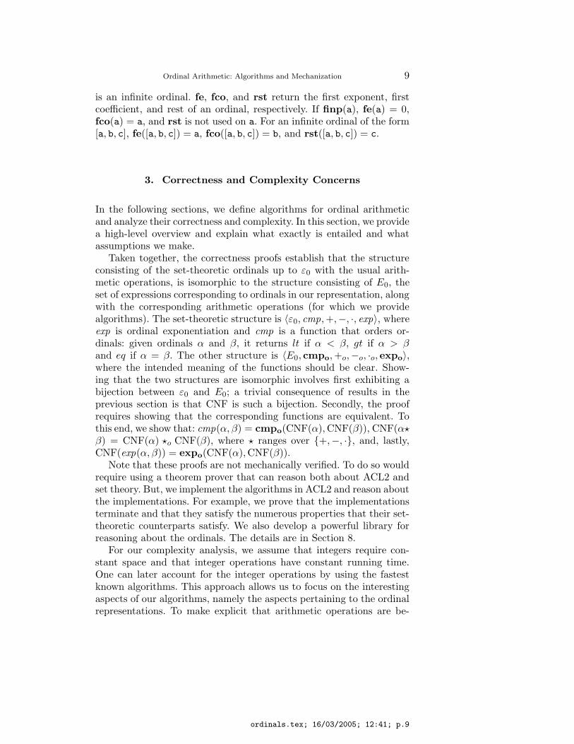
|a| {the length of a}finp(a) : 0

true : 1 + |rst(a)|

#a {the size of a}finp(a) : 1

true : #fe(a) + #rst(a)

Figure 1.: The length and size functions used for complexity analysis.

ing applied to integers, we refer to the usual arithmetic operations onintegers as <ω, +ω, −ω, ·ω, and expω.

The complexity of the ordinal arithmetic algorithms is given interms of the functions in Figure 1. In the figure, we use a sequenceof condition : result forms to define functions: the conditions shouldbe read from top to bottom until a condition that holds is found andthen the corresponding result is returned. Note that the true conditionalways holds. We use this format for definitions throughout the paper.

4. Comparing and Recognizing Ordinals

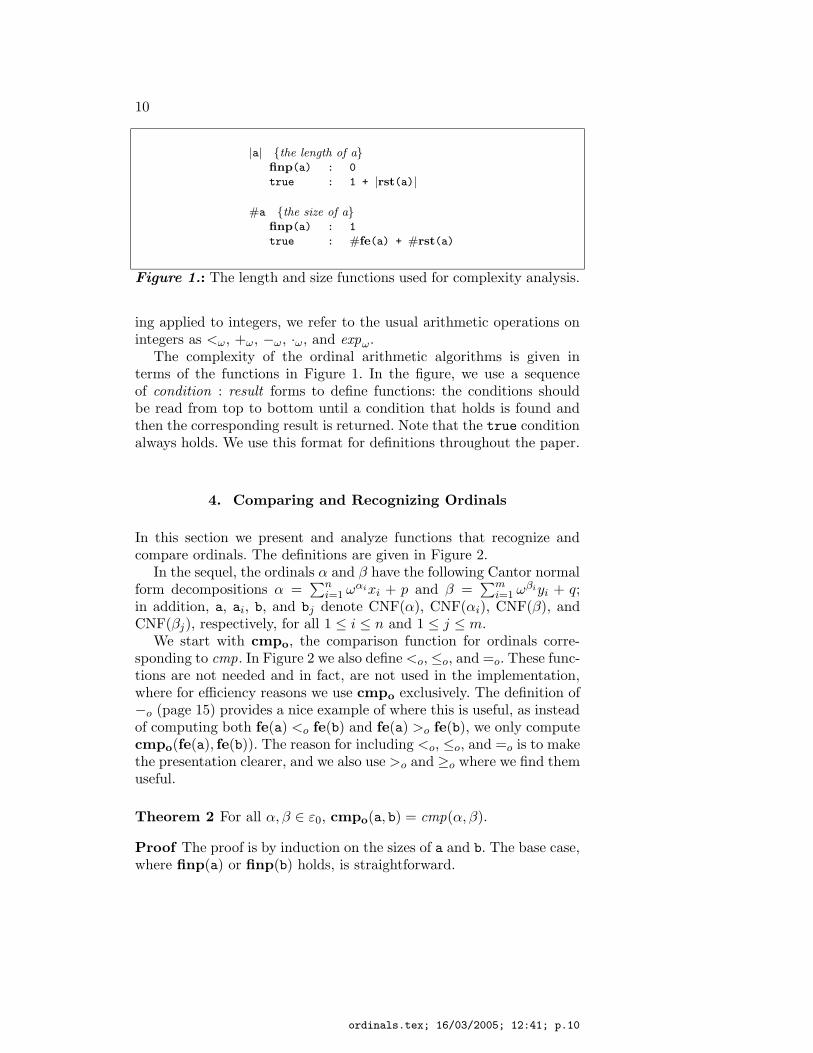
In this section we present and analyze functions that recognize andcompare ordinals. The definitions are given in Figure 2.

In the sequel, the ordinals α and β have the following Cantor normalform decompositions α =

∑ni=1 ωαixi + p and β =

∑mi=1 ωβiyi + q;

in addition, a, ai, b, and bj denote CNF(α), CNF(αi), CNF(β), andCNF(βj), respectively, for all 1 ≤ i ≤ n and 1 ≤ j ≤ m.

We start with cmpo, the comparison function for ordinals corre-sponding to cmp. In Figure 2 we also define <o, ≤o, and =o. These func-tions are not needed and in fact, are not used in the implementation,where for efficiency reasons we use cmpo exclusively. The definition of−o (page 15) provides a nice example of where this is useful, as insteadof computing both fe(a) <o fe(b) and fe(a) >o fe(b), we only computecmpo(fe(a), fe(b)). The reason for including <o, ≤o, and =o is to makethe presentation clearer, and we also use >o and ≥o where we find themuseful.

Theorem 2 For all α, β ∈ ε0, cmpo(a, b) = cmp(α, β).

Proof The proof is by induction on the sizes of a and b. The base case,where finp(a) or finp(b) holds, is straightforward.

ordinals.tex; 16/03/2005; 12:41; p.10

Ordinal Arithmetic: Algorithms and Mechanization 11

cmpω(p,q) {ordering on naturals}p <ω q : lt

q <ω p : gt

true : eq

cmpo(a,b) {ordering on ordinals}finp(a) ∧ finp(b) : cmpω(a,b)

finp(a) : lt

finp(b) : gt

cmpo(fe(a),fe(b)) 6= eq : cmpo(fe(a),fe(b))

cmpω(fco(a),fco(b)) 6= eq : cmpω(fco(a),fco(b))

true : cmpo(rst(a),rst(b))

a <o b {< for ordinals}cmpo(a,b) = lt : true

true : false

op(a) {ordinal recognizer}finp(a) : a ∈ ω

true : ¬finp(first(a))

∧ fco(a) ∈ ω

∧ 0 <ω fco(a)

∧ op(fe(a))

∧ op(rst(a))

∧ fe(rst(a)) <o fe(a)

a ≤o b {≤ for ordinals}cmpo(a,b) = gt : false

true : true

a =o b {= for ordinals}cmpo(a,b) = eq : true

true : false

Figure 2.: The ordinal ordering and recognizer algorithms.

For the induction step, we have that #a, #b > 1 and for all γ, δ if#CNF(γ) < #a and #CNF(δ) < #b, then cmpo(CNF(γ), CNF(δ))= cmp(γ, δ). There are 3 cases.

In the first, cmpo(a1, b1) 6= eq. If cmpo(a1, b1) = lt, then by the in-duction hypothesis, α1 < β1. Thus ωα1 < ωβ1 . Thus, since

∑ni=2 ωαixi <

ωα1 , α < ωβ1 ≤ β by the closure of additive principal ordinals under ad-dition. Therefore, cmp(α,β) = lt = cmpo(a, b). By a similar argument,cmpo(a1, b1) = gt ≡ cmp(α,β) = cmpo(a,b) = gt.

In the next case, we have that cmpo(a1, b1) = eq ∧ cmpω(x1, y1) 6=eq. By induction hypothesis, α1 = β1. Suppose that cmpω(x1, y1) = lt.

ordinals.tex; 16/03/2005; 12:41; p.11

12

Again, we note that∑n

i=2 ωαixi < ωα1 . Thus α < ωα1x1 + ωα1 , by thestrict right monotonicity of ordinal addition. But then we have

ωα1x1 + ωα1 = ωα1(x1 + 1) = ωβ1(x1 + 1) ≤ ωβ1y1

Hence, α < β, so cmpo(a1, b1) = lt = cmp(α, β). A similar argumentestablishes the case where cmpω(x1, y1) = gt.

In the final case, we have that cmpo(a1, b1) = eq ∧ cmpω(x1, y1) =eq. By the induction hypothesis, this means α1 = β1. If cmpo(rst(a),rst(b)) = eq, then by the induction hypothesis,

∑ni=2 ωαixi + p =

∑ni=2 ωβiyi + q and we have cmp(α, β) = eq = cmpo(a1, b1).If cmpo(rst(a), rst(b)) = lt, then by the induction hypothesis,

∑ni=2 ωαixi + p <

∑ni=2 ωβiyi + q; hence we have α < β. Therefore,

cmp(α, β) = lt = cmpo(a1, b1). A similar argument establishes thecase where cmpo(rst(a), rst(b)) = gt. �

Theorem 3 cmpo(a, b) runs in time O(min(#a, #b)).

Proof In the worst case we simultaneously recur down a and b. In moredetail, the complexity of this function is bounded by the recurrencerelation

T (a, b) =

{

c, if finp(a) or finp(b)T (a1, b1) + T (rst(a), rst(b)) + c, otherwise

for some constant value, c. It now follows by induction on the sizeof a and b that T (a, b) ≤ k · min(#a, #b) − t for any constants, k, t,such that t ≥ c and k ≥ c + t. �

We now analyze the complexity of op. At first glance it seemsthat the complexity is quadratic as op recurs both down the restof a (op(rst(a))) and into the exponent (op(a1)). However, a closerexamination reveals the following.

Theorem 4 op(a) runs in time O(#a(log #a)).

Proof The running time is bounded by the (non-linear) recurrencerelation

T (a) =

{

c, if finp(a)T (a1) + T (rst(a)) + min(#a1, #rst(a)) + c, otherwise

for some constant, c, by Theorem 3. We show by induction on #a, thatT (a) ≤ k(#a)(log #a) + t where k, t are constants such that t ≥ c andk ≥ 3t. In the base case, we have T (a) = c ≤ t. For the inductionstep, let x = min(#a1, #rst(a)) and y = max(#a1, #rst(a)). Note

ordinals.tex; 16/03/2005; 12:41; p.12

Ordinal Arithmetic: Algorithms and Mechanization 13

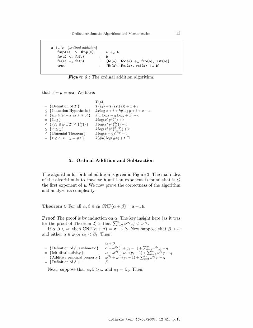
a +o b {ordinal addition}finp(a) ∧ finp(b) : a +ω b

fe(a) <o fe(b) : b

fe(a) =o fe(b) : [fe(a), fco(a) +ω fco(b), rst(b)]

true : [fe(a), fco(a), rst(a) +o b]

Figure 3.: The ordinal addition algorithm.

that x + y = #a. We have:

T (a)= {Definition of T } T (a1) + T (rst(a)) + x + c

≤ { Induction Hypothesis } kx log x + t + ky log y + t + x + c

≤ { kx ≥ 2t + x as k ≥ 3t } k(x log x + y log y + x) + c

= {Log } k log(xxyy2x) + c

≤ { 〈∀z ∈ ω :: 2z ≤(

2z

z

)

〉 } k log(xxyy(

2x

x

)

) + c

≤ {x ≤ y } k log(xxyy(

x+y

x

)

) + c

≤ {Binomial Theorem } k log(x + y)x+y + c

= { t ≥ c, x + y = #a } k(#a) log(#a) + t �

5. Ordinal Addition and Subtraction

The algorithm for ordinal addition is given in Figure 3. The main ideaof the algorithm is to traverse b until an exponent is found that is ≤the first exponent of a. We now prove the correctness of the algorithmand analyze its complexity.

Theorem 5 For all α, β ∈ ε0 CNF(α + β) = a +o b.

Proof The proof is by induction on α. The key insight here (as it wasfor the proof of Theorem 2) is that

∑ni=2 ωαixi < ωα1 .

If α, β ∈ ω, then CNF(α + β) = a +o b. Now suppose that β > ω

and either α ∈ ω or α1 < β1. Then:

α + β

= {Definition of β, arithmetic } α + ωβ1(1 + y1 − 1) +∑m

i=2 ωβiyi + q

= { left distributivity } α + ωβ1 + ωβ1(y1 − 1) +∑m

i=2 ωβiyi + q

= {Additive principal property } ωβ1 + ωβ1(y1 − 1) +∑m

i=2 ωβiyi + q

= {Definition of β } β

Next, suppose that α, β > ω and α1 = β1. Then:

ordinals.tex; 16/03/2005; 12:41; p.13

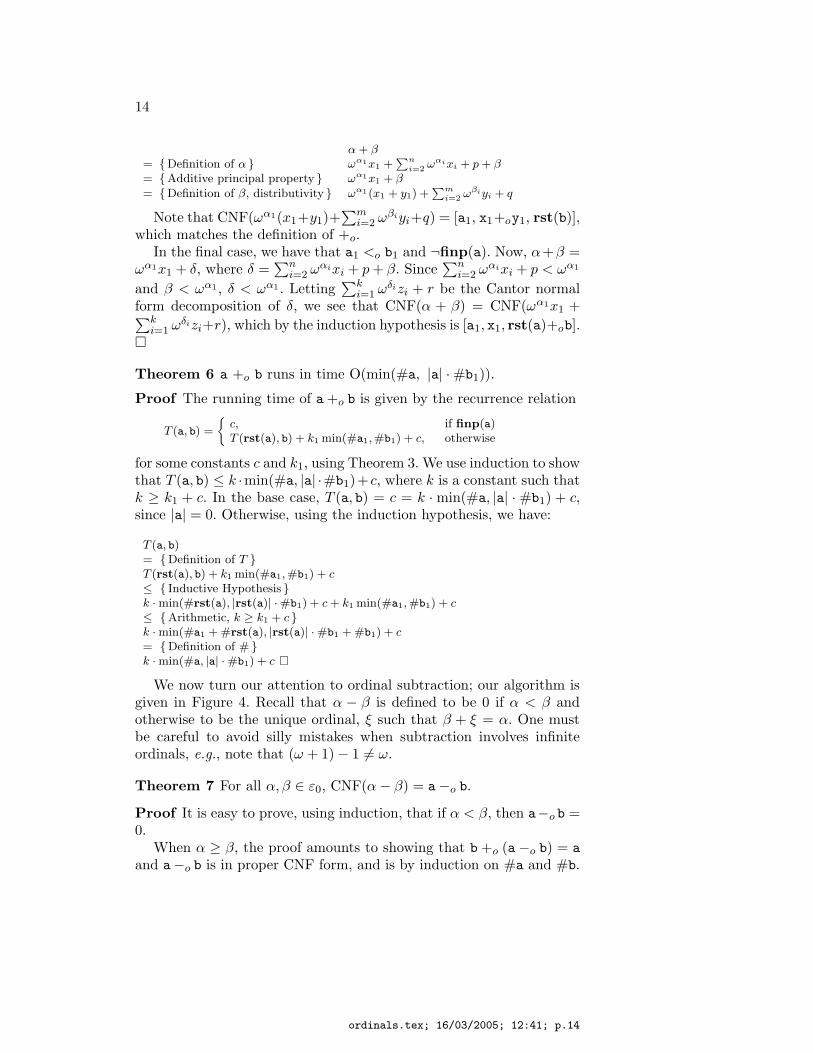
14

α + β

= {Definition of α } ωα1x1 +∑n

i=2 ωαixi + p + β

= {Additive principal property } ωα1x1 + β

= {Definition of β, distributivity } ωα1(x1 + y1) +∑m

i=2 ωβiyi + q

Note that CNF(ωα1(x1+y1)+∑m

i=2 ωβiyi+q) = [a1, x1+oy1, rst(b)],which matches the definition of +o.

In the final case, we have that a1 <o b1 and ¬finp(a). Now, α+β =ωα1x1 + δ, where δ =

∑ni=2 ωαixi + p + β. Since

∑ni=2 ωαixi + p < ωα1

and β < ωα1 , δ < ωα1 . Letting∑k

i=1 ωδizi + r be the Cantor normalform decomposition of δ, we see that CNF(α + β) = CNF(ωα1x1 +∑k

i=1 ωδizi+r), which by the induction hypothesis is [a1, x1, rst(a)+ob].�

Theorem 6 a +o b runs in time O(min(#a, |a| · #b1)).

Proof The running time of a +o b is given by the recurrence relation

T (a, b) =

{

c, if finp(a)T (rst(a), b) + k1 min(#a1, #b1) + c, otherwise

for some constants c and k1, using Theorem 3. We use induction to showthat T (a, b) ≤ k ·min(#a, |a| ·#b1)+c, where k is a constant such thatk ≥ k1 + c. In the base case, T (a, b) = c = k · min(#a, |a| · #b1) + c,since |a| = 0. Otherwise, using the induction hypothesis, we have:

T (a, b)= {Definition of T }T (rst(a), b) + k1 min(#a1, #b1) + c

≤ { Inductive Hypothesis }k · min(#rst(a), |rst(a)| · #b1) + c + k1 min(#a1, #b1) + c

≤ {Arithmetic, k ≥ k1 + c }k · min(#a1 + #rst(a), |rst(a)| · #b1 + #b1) + c

= {Definition of # }k · min(#a, |a| · #b1) + c �

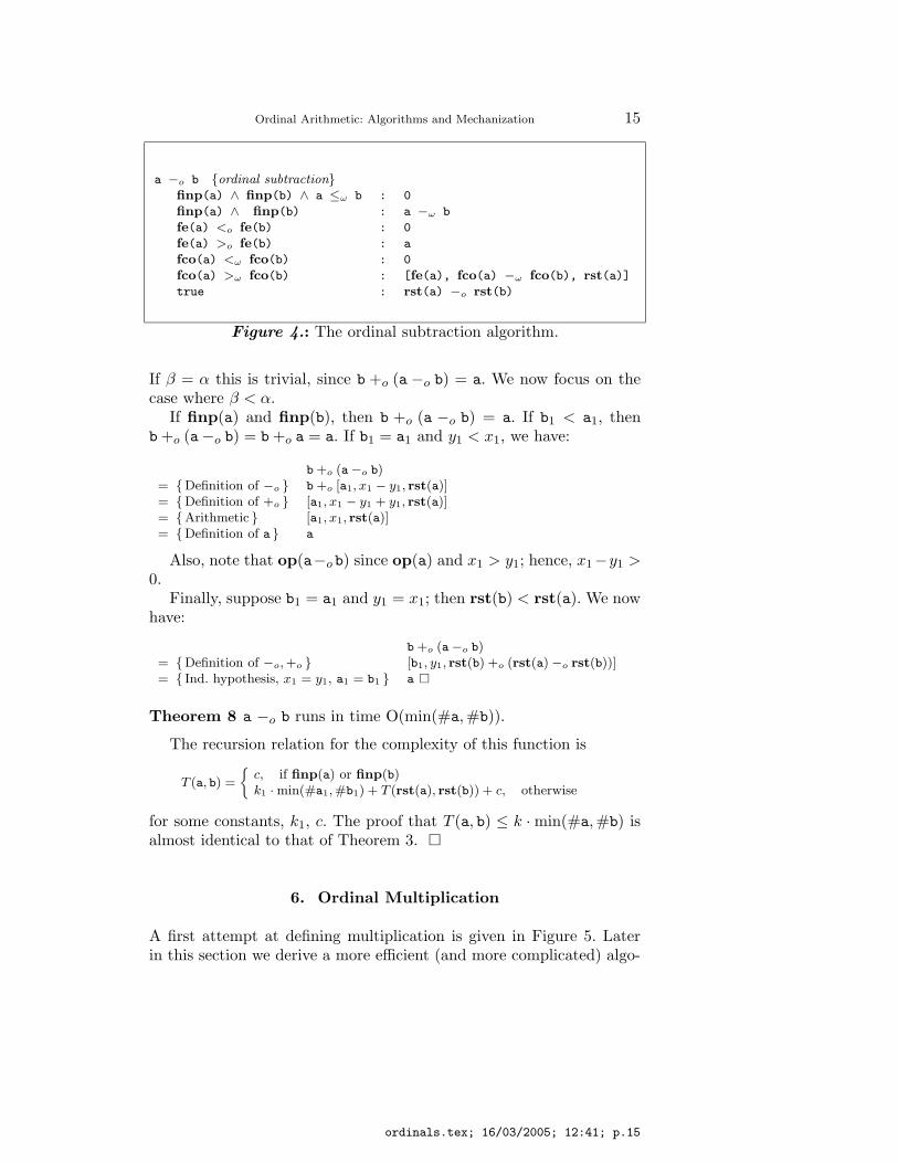
We now turn our attention to ordinal subtraction; our algorithm isgiven in Figure 4. Recall that α − β is defined to be 0 if α < β andotherwise to be the unique ordinal, ξ such that β + ξ = α. One mustbe careful to avoid silly mistakes when subtraction involves infiniteordinals, e.g., note that (ω + 1) − 1 6= ω.

Theorem 7 For all α, β ∈ ε0, CNF(α − β) = a−o b.

Proof It is easy to prove, using induction, that if α < β, then a−o b =0.

When α ≥ β, the proof amounts to showing that b +o (a−o b) = a

and a−o b is in proper CNF form, and is by induction on #a and #b.

ordinals.tex; 16/03/2005; 12:41; p.14

Ordinal Arithmetic: Algorithms and Mechanization 15

a −o b {ordinal subtraction}finp(a) ∧ finp(b) ∧ a ≤ω b : 0

finp(a) ∧ finp(b) : a −ω b

fe(a) <o fe(b) : 0

fe(a) >o fe(b) : a

fco(a) <ω fco(b) : 0

fco(a) >ω fco(b) : [fe(a), fco(a) −ω fco(b), rst(a)]

true : rst(a) −o rst(b)

Figure 4.: The ordinal subtraction algorithm.

If β = α this is trivial, since b +o (a −o b) = a. We now focus on thecase where β < α.

If finp(a) and finp(b), then b +o (a −o b) = a. If b1 < a1, thenb +o (a−o b) = b +o a = a. If b1 = a1 and y1 < x1, we have:

b +o (a−o b)= {Definition of −o } b +o [a1, x1 − y1, rst(a)]= {Definition of +o } [a1, x1 − y1 + y1, rst(a)]= {Arithmetic } [a1, x1, rst(a)]= {Definition of a } a

Also, note that op(a−o b) since op(a) and x1 > y1; hence, x1−y1 >

0.Finally, suppose b1 = a1 and y1 = x1; then rst(b) < rst(a). We now

have:

b +o (a−o b)= {Definition of −o, +o } [b1, y1, rst(b) +o (rst(a) −o rst(b))]= { Ind. hypothesis, x1 = y1, a1 = b1 } a �

Theorem 8 a −o b runs in time O(min(#a, #b)).

The recursion relation for the complexity of this function is

T (a, b) =

{

c, if finp(a) or finp(b)k1 · min(#a1, #b1) + T (rst(a), rst(b)) + c, otherwise

for some constants, k1, c. The proof that T (a, b) ≤ k · min(#a, #b) isalmost identical to that of Theorem 3. �

6. Ordinal Multiplication

A first attempt at defining multiplication is given in Figure 5. Laterin this section we derive a more efficient (and more complicated) algo-

ordinals.tex; 16/03/2005; 12:41; p.15

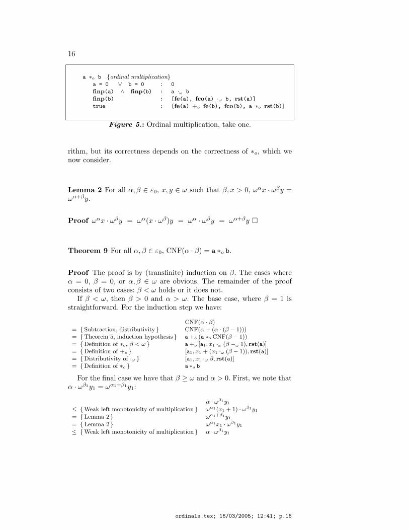
16

a ∗o b {ordinal multiplication}a = 0 ∨ b = 0 : 0

finp(a) ∧ finp(b) : a ·ω b

finp(b) : [fe(a), fco(a) ·ω b, rst(a)]

true : [fe(a) +o fe(b), fco(b), a ∗o rst(b)]

Figure 5.: Ordinal multiplication, take one.

rithm, but its correctness depends on the correctness of ∗o, which wenow consider.

Lemma 2 For all α, β ∈ ε0, x, y ∈ ω such that β, x > 0, ωαx · ωβy =ωα+βy.

Proof ωαx · ωβy = ωα(x · ωβ)y = ωα · ωβy = ωα+βy �

Theorem 9 For all α, β ∈ ε0, CNF(α · β) = a ∗o b.

Proof The proof is by (transfinite) induction on β. The cases whereα = 0, β = 0, or α, β ∈ ω are obvious. The remainder of the proofconsists of two cases: β < ω holds or it does not.

If β < ω, then β > 0 and α > ω. The base case, where β = 1 isstraightforward. For the induction step we have:

CNF(α · β)= {Subtraction, distributivity } CNF(α + (α · (β − 1)))= {Theorem 5, induction hypothesis } a +o (a ∗o CNF(β − 1))= {Definition of ∗o, β < ω } a +o [a1, x1 ·ω (β −ω 1), rst(a)]= {Definition of +o } [a1, x1 + (x1 ·ω (β − 1)), rst(a)]= {Distributivity of ·ω } [a1, x1 ·ω β, rst(a)]= {Definition of ∗o } a ∗o b

For the final case we have that β ≥ ω and α > 0. First, we note thatα · ωβ1y1 = ωα1+β1y1:

α · ωβ1y1

≤ {Weak left monotonicity of multiplication } ωα1(x1 + 1) · ωβ1y1

= {Lemma 2 } ωα1+β1y1

= {Lemma 2 } ωα1x1 · ωβ1y1

≤ {Weak left monotonicity of multiplication } α · ωβ1y1

ordinals.tex; 16/03/2005; 12:41; p.16

Ordinal Arithmetic: Algorithms and Mechanization 17

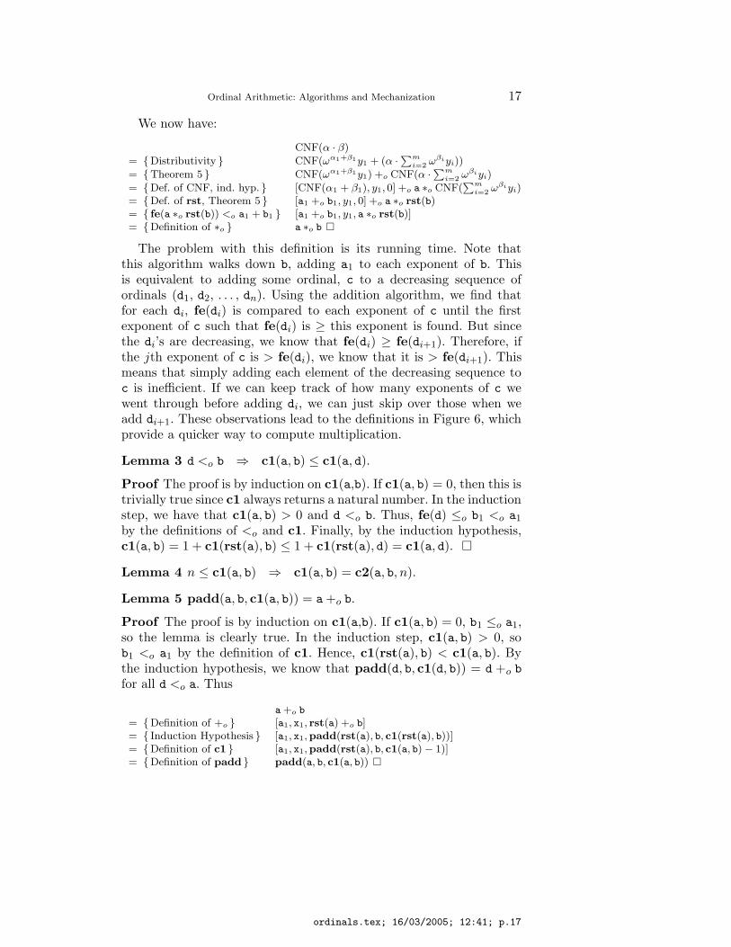
We now have:

CNF(α · β)

= {Distributivity } CNF(ωα1+β1y1 + (α ·∑m

i=2 ωβiyi))

= {Theorem 5 } CNF(ωα1+β1y1) +o CNF(α ·∑m

i=2 ωβiyi)

= {Def. of CNF, ind. hyp. } [CNF(α1 + β1), y1, 0] +o a ∗o CNF(∑m

i=2 ωβiyi)= {Def. of rst, Theorem 5 } [a1 +o b1, y1, 0] +o a ∗o rst(b)= { fe(a ∗o rst(b)) <o a1 + b1 } [a1 +o b1, y1, a ∗o rst(b)]= {Definition of ∗o } a ∗o b �

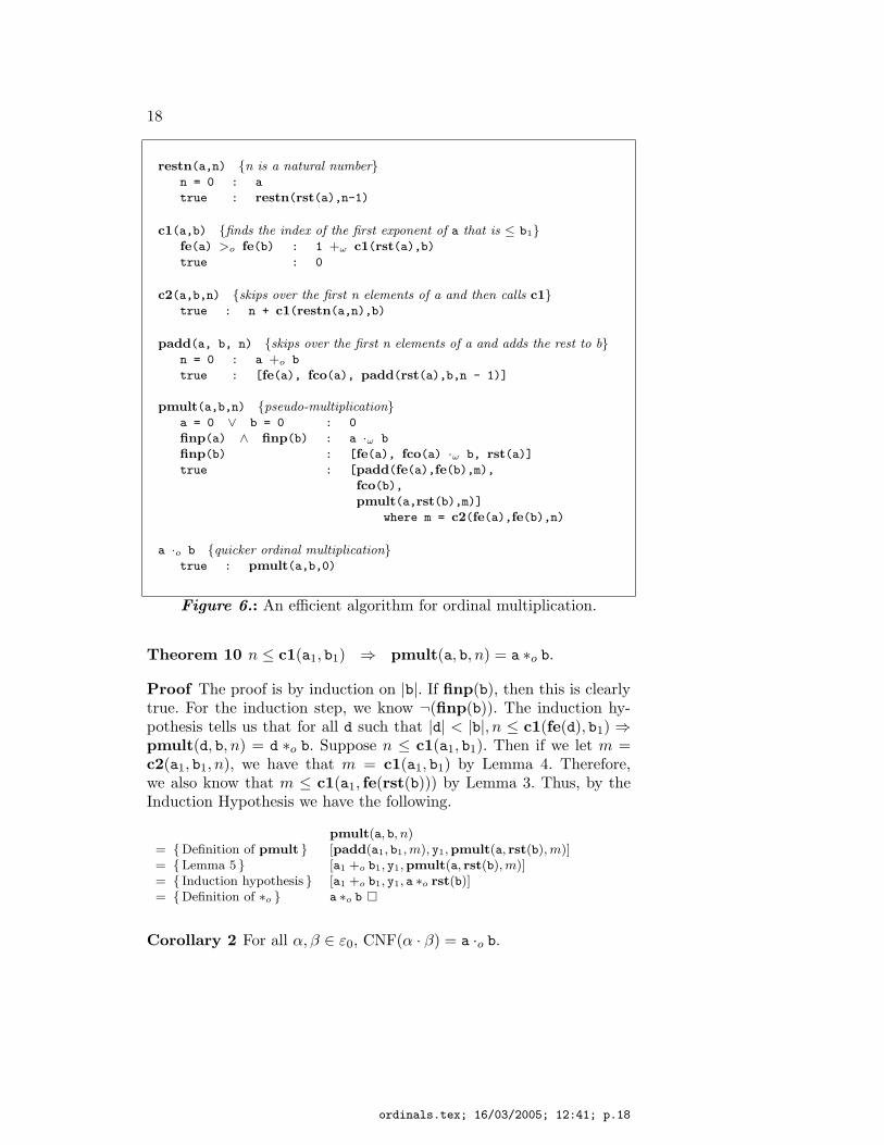
The problem with this definition is its running time. Note thatthis algorithm walks down b, adding a1 to each exponent of b. Thisis equivalent to adding some ordinal, c to a decreasing sequence ofordinals (d1, d2, . . . , dn). Using the addition algorithm, we find thatfor each di, fe(di) is compared to each exponent of c until the firstexponent of c such that fe(di) is ≥ this exponent is found. But sincethe di’s are decreasing, we know that fe(di) ≥ fe(di+1). Therefore, ifthe jth exponent of c is > fe(di), we know that it is > fe(di+1). Thismeans that simply adding each element of the decreasing sequence toc is inefficient. If we can keep track of how many exponents of c wewent through before adding di, we can just skip over those when weadd di+1. These observations lead to the definitions in Figure 6, whichprovide a quicker way to compute multiplication.

Lemma 3 d <o b ⇒ c1(a, b) ≤ c1(a, d).

Proof The proof is by induction on c1(a,b). If c1(a, b) = 0, then this istrivially true since c1 always returns a natural number. In the inductionstep, we have that c1(a, b) > 0 and d <o b. Thus, fe(d) ≤o b1 <o a1

by the definitions of <o and c1. Finally, by the induction hypothesis,c1(a, b) = 1 + c1(rst(a), b) ≤ 1 + c1(rst(a), d) = c1(a, d). �

Lemma 4 n ≤ c1(a, b) ⇒ c1(a, b) = c2(a, b, n).

Lemma 5 padd(a, b, c1(a, b)) = a +o b.

Proof The proof is by induction on c1(a,b). If c1(a, b) = 0, b1 ≤o a1,so the lemma is clearly true. In the induction step, c1(a, b) > 0, sob1 <o a1 by the definition of c1. Hence, c1(rst(a), b) < c1(a, b). Bythe induction hypothesis, we know that padd(d, b, c1(d, b)) = d +o b

for all d <o a. Thus

a +o b

= {Definition of +o } [a1, x1, rst(a) +o b]= { Induction Hypothesis } [a1, x1,padd(rst(a), b, c1(rst(a), b))]= {Definition of c1 } [a1, x1,padd(rst(a), b, c1(a, b) − 1)]= {Definition of padd } padd(a, b, c1(a, b)) �

ordinals.tex; 16/03/2005; 12:41; p.17

18

restn(a,n) {n is a natural number}n = 0 : a

true : restn(rst(a),n-1)

c1(a,b) {finds the index of the first exponent of a that is ≤ b1}fe(a) >o fe(b) : 1 +ω c1(rst(a),b)

true : 0

c2(a,b,n) {skips over the first n elements of a and then calls c1}true : n + c1(restn(a,n),b)

padd(a, b, n) {skips over the first n elements of a and adds the rest to b}n = 0 : a +o b

true : [fe(a), fco(a), padd(rst(a),b,n - 1)]

pmult(a,b,n) {pseudo-multiplication}a = 0 ∨ b = 0 : 0

finp(a) ∧ finp(b) : a ·ω b

finp(b) : [fe(a), fco(a) ·ω b, rst(a)]

true : [padd(fe(a),fe(b),m),

fco(b),

pmult(a,rst(b),m)]

where m = c2(fe(a),fe(b),n)

a ·o b {quicker ordinal multiplication}true : pmult(a,b,0)

Figure 6.: An efficient algorithm for ordinal multiplication.

Theorem 10 n ≤ c1(a1, b1) ⇒ pmult(a, b, n) = a ∗o b.

Proof The proof is by induction on |b|. If finp(b), then this is clearlytrue. For the induction step, we know ¬(finp(b)). The induction hy-pothesis tells us that for all d such that |d| < |b|, n ≤ c1(fe(d), b1) ⇒pmult(d, b, n) = d ∗o b. Suppose n ≤ c1(a1, b1). Then if we let m =c2(a1, b1, n), we have that m = c1(a1, b1) by Lemma 4. Therefore,we also know that m ≤ c1(a1, fe(rst(b))) by Lemma 3. Thus, by theInduction Hypothesis we have the following.

pmult(a, b, n)= {Definition of pmult } [padd(a1, b1, m), y1,pmult(a, rst(b), m)]= {Lemma 5 } [a1 +o b1, y1,pmult(a, rst(b), m)]= { Induction hypothesis } [a1 +o b1, y1, a ∗o rst(b)]= {Definition of ∗o } a ∗o b �

Corollary 2 For all α, β ∈ ε0, CNF(α · β) = a ·o b.

ordinals.tex; 16/03/2005; 12:41; p.18

Ordinal Arithmetic: Algorithms and Mechanization 19

Proof Follows directly from Theorems 9 and 10. �

We now turn our attention to complexity issues. For the next lemmasand theorem, let a1 = [d1, z1, [d2, z2, . . . [dk, zk, r] . . .]].

Lemma 6 c1(a, b) takes time O(∑c1(a,b)+1

i=1 min(#ai, #b1)).

Proof In the worst case, we traverse a, comparing ai with b1. By

Theorem 3, this takes O(∑c1(a,b)+1

i=1 min(#ai, #b1)) time. �

Lemma 7 c2(a, b, s) takes time O(s +∑c1(a,b)+1

i=s+1 min(#ai, #b1)).

Lemma 8 padd(a, b, s) runs in time O(min(#fe(restn(a, s)), #b1) +s) when s ≥ c1(a, b).

Proof Note that fe(restn(a, s)) ≤ b1 since the exponents of a are de-creasing and s ≥ c1(a,b). Hence, restn(a, s)+o b requires one compar-ison and creates an answer in constant time. Therefore, by Theorem 3,padd takes O(min(#fe(restn(a, s)), #b1) + s) time. �

Theorem 11 pmult(a, b, s) runs in time O(|a1||b| + #restn(a1, s) +#b) if s ≤ c1(a1, b1).

Proof Let m = c2(a1, b1, s); then m = c1(a1, b1) by Lemma 4. Thus,using Lemmas 7 and 8, we can construct the following recurrencerelation to bound the running time of pmult:

T (a, b, s) =

d, if finp(b) ∨ a= 0

T (a, rst(b), m) + k1(s +∑m+1

i=s+1 min(#di, #fe(b1)))+k2(min(#fe(restn(a1, m)), #b1) + m) + d, otherwise

for some constants k1, k2, and d. We use induction on |b| to show thatT (a, b, s) ≤ k ·(|a1||b|+#restn(a1, s)+#b) where k ≥ k1+k2+d. Thisis true in the base case, because #b = 1 and k ≥ d. For the inductionstep, we first note the following.

k1[s +∑m+1

i=s+1 min(#di, #fe(b1))] + k2[min(#fe(restn(a, m)), #fe(b1)) + m] + d

≤ {Arithmetic, m ≥ s }k1(m +

∑m

i=s+1 #di + #fe(b1)) + (k2 + d)(#fe(b1) + m)≤ { k ≥ k1 + k2 + d }k(m +

∑m

i=s+1 #di + #fe(b1))

ordinals.tex; 16/03/2005; 12:41; p.19

20

exp1(k,a) {raising a positive integer to an infinite ordinal power}fe(a) =o 1 : [fco(a), expω(k,rst(a)), 0]

finp(rst(a)) : [[fe(a) −o 1, fco(a), 0], expω(k,rst(a)), 0]

true : [[fe(a) −o 1, 1, fe(c)], fco(c), 0]

where c = exp1(k,rst(a))

Figure 7.: Ordinal exponentiation: raising a positive integer to aninfinite power.

Combining this with the recurrence relation and using the inductionhypothesis, we have:

T (a, b, s)≤ {Definition of T , earlier reasoning }T (a, rst(b), m) + k(m +

∑m

i=s+1 #di + #fe(b1))≤ { Induction Hypothesis }k(|a1||rst(b)| + #restn(a1, m) + #rst(b) + m +

∑m

i=s+1 #di + #fe(b1)) + d

≤ {Arithmetic, m ≤ |a1| }k(|a1||b| + #restn(a1, m) +

∑m

i=s+1 #di + #rst(b) + #fe(b1)) + d

= {Definitions of #, restn }k(|a1||b| + #restn(a1, s) + #rst(b) + #fe(b1)) + d

< {#fe(b1) < #b1 }k(|a1||b| + #restn(a1, s) + #b) + d �

Corollary 3 a ·o b runs in time O(|a1||b| + #a1 + #b).

7. Ordinal Exponentiation

Ordinal exponentiation is more complex than ordinal multiplication,and in an effort to increase clarity, we define exponentiation (expo)using four helper functions: exp1, exp2, exp3, and exp4. We introducethem one at a time, proving the correctness and complexity of eachbefore moving on to the next. The correctness and complexity of expo

come at the end and follow directly from the results proved for thehelper functions. Before reading further, the reader may want to try afew examples; a particularly revealing class of examples is (ω +1)ωω+k,where k ranges over the naturals.

The first helper function, exp1, is defined in Figure 7, and it is usedto raise a positive integer to an infinite ordinal power. We proceed byproving that it is correct and analyzing its complexity.

Lemma 9 ∀k, x ∈ ω, α ∈ ε0 such that α > 0, x > 0, and k > 1,kωαx = ωωα−1x

ordinals.tex; 16/03/2005; 12:41; p.20

Ordinal Arithmetic: Algorithms and Mechanization 21

Proof kωαx = kω1+α−1x = kω·ωα−1x = (kω)ωα−1x = ωωα−1x�

Lemma 10 ∀k ∈ ω, α ∈ ε0 such that α > 0 and k > 1, kα =(ω

∑ni=1 ωαi−1xi)kp

Proof Recall that the Cantor normal form decomposition of α is∑n

i=1 ωαixi + p. The proof follows from Lemma 9. �

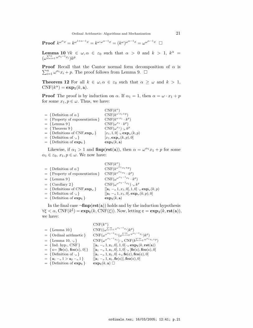
Theorem 12 For all k ∈ ω, α ∈ ε0 such that α ≥ ω and k > 1,CNF(kα) = exp1(k, a).

Proof The proof is by induction on α. If α1 = 1, then α = ω · x1 + p

for some x1, p ∈ ω. Thus, we have:

CNF(kα)= {Definition of α } CNF(kω·x1+p)= {Property of exponentiation } CNF(kω·x1 · kp)= {Lemma 9 } CNF(ωx1 · kp)= {Theorem 9 } CNF(ωx1) ·o kp

= {Definitions of CNF,expω } [x1, 1, 0] ·o expω(k, p)= {Definition of ·o } [x1, expω(k, p), 0]= {Definition of exp1 } exp1(k, a)

Likewise, if α1 > 1 and finp(rst(a)), then α = ωα1x1 + p for someα1 ∈ ε0, x1, p ∈ ω. We now have:

CNF(kα)

= {Definition of α } CNF(kωα1x1+p)

= {Property of exponentiation } CNF(kωα1x1 · kp)

= {Lemma 9 } CNF(ωωα1−1x1 · kp)

= {Corollary 2 } CNF(ωωα1−1x1) ·o kp

= {Definitions of CNF,expω } [[a1 −o 1, x1, 0], 1, 0] ·o expω(k, p)= {Definition of ·o } [[a1 −o 1, x1, 0], expω(k, p), 0]= {Definition of exp1 } exp1(k, a)

In the final case ¬finp(rst(a)) holds and by the induction hypothesis∀ξ < α, CNF(kξ) = exp1(k, CNF(ξ)). Now, letting c = exp1(k, rst(a)),we have:

CNF(kα)

= {Lemma 10 } CNF((ω∑m

i=1ωαi−1xi)kp)

= {Ordinal arithmetic } CNF(ωωα1−1x1(ω∑m

i=2wαi−1xi)kp)

= {Lemma 10, ·o } CNF(ωωα1−1x1) ·o CNF(k∑m

i=2wαi xi+p)

= { Ind. hyp., CNF } [[a1 −o 1, x1, 0], 1, 0] ·o exp1(k, rst(a))= { c= [fe(c), fco(c), 0] } [[a1 −o 1, x1, 0], 1, 0] ·o [fe(c), fco(c), 0]= {Definition of ·o } [[a1 −o 1, x1, 0] +o fe(c), fco(c), 0]= { a1 −o 1 > a2 −o 1 } [[a1 −o 1, x1, fe(c)], fco(c), 0]= {Definition of exp1 } exp1(k, a) �

ordinals.tex; 16/03/2005; 12:41; p.21

22

exp2(a,k) {raising a limit ordinal to a positive integer}true : [fe(a) ·o (k - 1), 1, 0] ·o a

natpart(a) {returns the natural part of an ordinal}finp(a) : a

true : natpart(rst(a))

limitp(a) {returns true if a represents a limit ordinal}true : op(a) ∧ ¬finp(a) ∧ natpart(a) = 0

limitpart(a) {returns the greatest ordinal, b, such that limitp(b) and b <o a}finp(a) : 0

true : [fe(a), fco(a), limitpart(rst(a))]

Figure 8.: Ordinal exponentiation: raising a limit ordinal to a positiveinteger.

Theorem 13 exp1 runs in time O(|a|).

Proof Note that by Theorem 8, computing a1−o1 takes constant time.The proof is now straightforward. �

We now consider the second helper function, exp2, which is shownin Figure 8 and is used to raise a limit ordinal to a positive integer.

Lemma 11 For all a, b such that op(a), op(b), natpart(b) = 0 and¬finp(a), a ·o b = [a1, 1, 0] ·o b.

Proof The proof is by induction on |b|. If finp(b), then b = 0 anda ·o b = 0 = [a1, 1, 0] ·o b. For the induction step we have:

a ·o b= {Definition of ·o } [a1 + b1, y1, a ·o rst(b)]= { Induction Hypothesis } [a1 + b1, y1, [a1, 1, 0] ·o rst(b)]= {Definition of ·o } [a1, 1, 0] ·o b �

Theorem 14 For all α ∈ ε0, k ∈ ω such that α ≥ ω, limitp(a), andk > 1, CNF(αk) = exp2(a, k).

Proof The proof is by induction on k. If k = 2, then CNF(αk) =CNF(α2) = CNF(α ·α) = a ·o a. Applying Lemma 11, we get [a1, 1, 0] ·o

ordinals.tex; 16/03/2005; 12:41; p.22

Ordinal Arithmetic: Algorithms and Mechanization 23

exp3h(a,p,n,k) {helper function for exp3}k = 1 : (a ·o p) +o p

true : padd(exp2(a,k) ·o p, exp3h(a,p,n,k-1), n)

exp3(a,k) {raising an infinite ordinal to a positive integer power}k = 1 : a

limitp(a) : exp2(a,k)

true : padd(exp2(c,k),

exp3h(c,natpart(a),n,k-1),

n)

where c = limitpart(a) and n = |a|

Figure 9.: Ordinal exponentiation: raising an infinite ordinal to apositive integer power.

a = exp2(a, k). For the induction step we have:

CNF(αk)

= {Ordinal arithmetic, ·o } a ·o CNF(αk−1)= { Induction hypothesis } a ·o exp2(a, k − 1)= {Definition of exp2 } a ·o [a1 ·o (k − 2), 1, 0] ·o a= {Definition of ·o } [a1 +o (a1 ·o (k − 2)), 1, 0] ·o a= {Distr., Theorem 5, Corollary 2 } [a1 ·o (k − 1), 1, 0] ·o a= {Definition of exp2 } exp2(a, k) �

Theorem 15 exp2(a, k) runs in time O(|a1||a| + #a)

Proof Note that a1 ·o (k − 1) takes constant time, since k − 1 is ofsize 1. Also, note that #(a1 ·o (k − 1)) = #a1 and |a1 ·o (k − 1)| = |a1|.So, by Corollary 3, we have that the running time is O(|a1||a|+#a). �

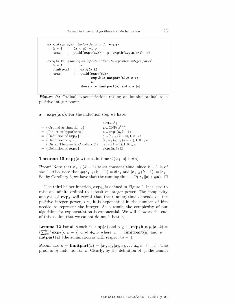
The third helper function, exp3, is defined in Figure 9. It is used toraise an infinite ordinal to a positive integer power. The complexityanalysis of exp3 will reveal that the running time depends on thepositive integer power, i.e., it is exponential in the number of bitsneeded to represent the integer. As a result, the complexity of ouralgorithm for exponentiation is exponential. We will show at the endof this section that we cannot do much better.

Lemma 12 For all a such that op(a) and α ≥ ω, exp3h(c, p, |a|, k) =

(∑k−1

i=0 exp2(c, k − i) ·o p) +o p where c = limitpart(a) and p =natpart(a) (the summation is with respect to +o).

Proof Let c = limitpart(a) = [a1, x1, [a2, x2, . . . [an, xn, 0] . . .]]. Theproof is by induction on k. Clearly, by the definition of ·o, the lemma

ordinals.tex; 16/03/2005; 12:41; p.23

24

holds when k = 1. For the induction step we have:

exp3h(c, p, n, k)= {Definition of exp3h }padd(exp2(c, k) ·o p, exp3h(a, p, n, k − 1), n)= { Induction hypothesis, arithmetic }

padd(exp2(c, k) ·o p, (∑k−1

i=1 exp2(c, k − i) ·o p) +o p, n)= { See immediately below }

(∑k−1

i=0 exp2(c, k − i) ·o p) +o p

We justify the last step of the above proof by noting that:

exp2(c, k) ·o p = [a1 ·o x+o a1, x1 · p, [a1 ·o x+o a2, x2, . . . [a1 ·o x+o an, xn, 0] . . .]]

where x = k − 1. That is, by the definition of exp3h, we have thatfe(exp3h(a, p, n, k − 1)) = (a1 ·o (k − 1)); thus, every exponent inexp2(c, k) ·op is greater than the first exponent of exp3h(a, p, n, k−1).�

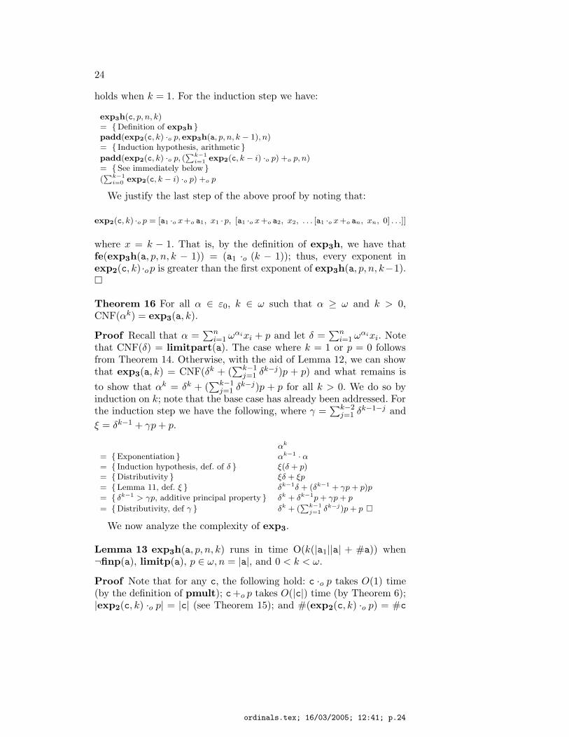
Theorem 16 For all α ∈ ε0, k ∈ ω such that α ≥ ω and k > 0,CNF(αk) = exp3(a, k).

Proof Recall that α =∑n

i=1 ωαixi + p and let δ =∑n

i=1 ωαixi. Notethat CNF(δ) = limitpart(a). The case where k = 1 or p = 0 followsfrom Theorem 14. Otherwise, with the aid of Lemma 12, we can showthat exp3(a, k) = CNF(δk + (

∑k−1j=1 δk−j)p + p) and what remains is

to show that αk = δk + (∑k−1

j=1 δk−j)p + p for all k > 0. We do so byinduction on k; note that the base case has already been addressed. Forthe induction step we have the following, where γ =

∑k−2j=1 δk−1−j and

ξ = δk−1 + γp + p.

αk

= {Exponentiation } αk−1 · α= { Induction hypothesis, def. of δ } ξ(δ + p)= {Distributivity } ξδ + ξp

= {Lemma 11, def. ξ } δk−1δ + (δk−1 + γp + p)p

= { δk−1 > γp, additive principal property } δk + δk−1p + γp + p

= {Distributivity, def γ } δk + (∑k−1

j=1 δk−j)p + p �

We now analyze the complexity of exp3.

Lemma 13 exp3h(a, p, n, k) runs in time O(k(|a1||a| + #a)) when¬finp(a), limitp(a), p ∈ ω, n = |a|, and 0 < k < ω.

Proof Note that for any c, the following hold: c ·o p takes O(1) time(by the definition of pmult); c+o p takes O(|c|) time (by Theorem 6);|exp2(c, k) ·o p| = |c| (see Theorem 15); and #(exp2(c, k) ·o p) = #c

ordinals.tex; 16/03/2005; 12:41; p.24

Ordinal Arithmetic: Algorithms and Mechanization 25

exp4(a,b) {raising an infinite ordinal to an infinite power}true : [fe(a) ·o limitpart(b), 1, 0] ·o exp3(a,natpart(b))

expo(a,b) {ordinal exponentiation (raises a to the b power)}b = 0 ∨ a = 1 : 1

a = 0 : 0

finp(a) ∧ finp(b) : expω(a,b)

finp(a) : exp1(a,b)

finp(b) : exp3(a,b)

true : exp4(a,b)

Figure 10.: The ordinal exponentiation algorithm.

(again, see Theorem 15). Now, exp3h gets called O(k) times and eachcall requires O(|a1||a|+ #a+ |a|) time. Therefore, by Theorem 15 andthe above observations, the total time is O(k(|a1||a| + #a)). �

Theorem 17 exp3(a, k) runs in time O(k · (|a1||a| + #a)).

Proof This is a straightforward consequence of Lemma 13 and Theo-rem 15. �

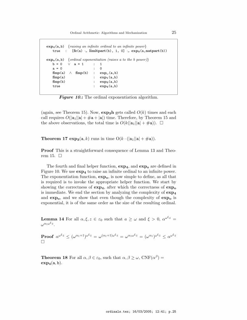
The fourth and final helper function, exp4, and expo are defined inFigure 10. We use exp4 to raise an infinite ordinal to an infinite power.The exponentiation function, expo, is now simple to define, as all thatis required is to invoke the appropriate helper function. We start byshowing the correctness of exp4, after which the correctness of expo

is immediate. We end the section by analyzing the complexity of exp4

and expo, and we show that even though the complexity of expo isexponential, it is of the same order as the size of the resulting ordinal.

Lemma 14 For all α, ξ, z ∈ ε0 such that a ≥ ω and ξ > 0, αωξz =

ωα1ωξz.

Proof αωξz ≤ (ωα1+1)ωξz = ω(α1+1)ωξz = ωα1ωξz = (ωα1)ωξz ≤ αωξz

�

Theorem 18 For all α, β ∈ ε0, such that α, β ≥ ω, CNF(αβ) =exp4(a, b).

ordinals.tex; 16/03/2005; 12:41; p.25

26

Proof

CNF(αβ)

= {Def. of β } CNF(α∑m

i=1ωβi yi+q)

= {Ordinal arithmetic } CNF(∏m

i=1αωβi yi · αq)

= {Lemma 14 } CNF(∏m

i=1ωα1·ω

βi yi · αq)

= {Property of exponentiation } CNF(ωα1·

∑mi=1

ωβi yi · αq)= {Theorem 16, Corollary 2 } [a1 ·o limitpart(b), 1, 0] ·o exp2(a, q)= {Definition exp4 } exp4(a, b) �

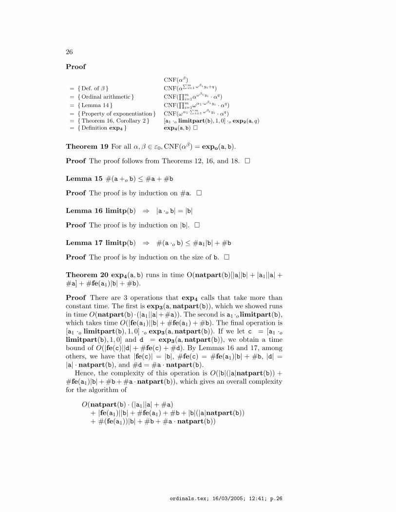
Theorem 19 For all α, β ∈ ε0, CNF(αβ) = expo(a, b).

Proof The proof follows from Theorems 12, 16, and 18. �

Lemma 15 #(a +o b) ≤ #a + #b

Proof The proof is by induction on #a. �

Lemma 16 limitp(b) ⇒ |a ·o b| = |b|

Proof The proof is by induction on |b|. �

Lemma 17 limitp(b) ⇒ #(a ·o b) ≤ #a1|b| + #b

Proof The proof is by induction on the size of b. �

Theorem 20 exp4(a, b) runs in time O(natpart(b)[|a||b| + |a1||a| +#a] + #fe(a1)|b| + #b).

Proof There are 3 operations that exp4 calls that take more thanconstant time. The first is exp3(a,natpart(b)), which we showed runsin time O(natpart(b) ·(|a1||a|+#a)). The second is a1 ·o limitpart(b),which takes time O(|fe(a1)||b|+ #fe(a1) + #b). The final operation is[a1 ·o limitpart(b), 1, 0] ·o exp3(a,natpart(b)). If we let c = [a1 ·olimitpart(b), 1, 0] and d = exp3(a,natpart(b)), we obtain a timebound of O(|fe(c)||d| + #fe(c) + #d). By Lemmas 16 and 17, amongothers, we have that |fe(c)| = |b|, #fe(c) = #fe(a1)|b| + #b, |d| =|a| · natpart(b), and #d = #a · natpart(b).

Hence, the complexity of this operation is O(|b|(|a|natpart(b)) +#fe(a1)|b|+ #b+ #a ·natpart(b)), which gives an overall complexityfor the algorithm of

O(natpart(b) · (|a1||a| + #a)+ |fe(a1)||b| + #fe(a1) + #b + |b|(|a|natpart(b))+ #(fe(a1))|b| + #b + #a · natpart(b))

ordinals.tex; 16/03/2005; 12:41; p.26

Ordinal Arithmetic: Algorithms and Mechanization 27

By gathering like terms and noting that #(fe(a1))|b| > |fe(a1)||b|, weobtain a time bound of O(natpart(b)[|a||b|+|a1||a|+#a]+#fe(a1)|b|+#b). �

Theorem 21 expo(a, b) runs in time O(natpart(b)[|a||b| + |a1||a| +#a] + #fe(a1)|b| + #b).

Proof This follows directly from Theorems 13, 17, and 20. �

An obvious question is whether we can improve the exponentialrunning time of expo. Given our representation of the ordinals, theanswer is no, as the following class of examples shows. Fix a to be [1,1, 1], which corresponds to the ordinal ω + 1 and let bk be [[1, 1, 1],1, k], which corresponds to the ordinal ωω + k. For this infinite classof examples, #expo(a, bk) is exactly equal to the complexity of expo.That is, simply constructing the ordinal corresponding to expo(a, bk)takes as long as this function takes to run in the worst case. Therefore,this algorithm is as efficient as can be expected.

8. Implementation

In this section, we describe the implementation of the ordinal arithmeticalgorithms in the ACL2 theorem proving system. There are severalfacets to this work. In Section 8.1, we give a brief overview of ACL2and describe the ACL2 implementation of the ordinal arithmetic al-gorithms. In Section 8.2, we discuss the mechanical verification of theimplementations. The proof scripts are part of the ACL2 distribution(as of version 2.8) and are described in greater detail elsewhere [37]. Ourmain goal in formalizing ordinal arithmetic on ordinal notations wasto enable ACL2 to automatically prove complex theorems involvingthe ordinals. In Section 8.3, we give an overview of the library weengineered into a tool for reasoning about termination and the ordinalsin ACL2, and we give an example of their use. Our treatment of theordinals provides many advantages over the treatment in ACL2 v2.7;thus, we decided to update the representations, definitions, theorems,and documentation of the ordinals [38]. These modification are presentin ACL2 version 2.8 and include a more efficient ordinal representationand a greatly extended ability to reason about ordinals. This aspect ofour work is described in Section 8.4.

ordinals.tex; 16/03/2005; 12:41; p.27

28

8.1. Implementation in ACL2

“ACL2” stands for “A Computational Logic for Applicative CommonLisp.” It is the name of a programming language, a first-order mathe-matical logic based on recursive functions, and a mechanical theoremprover for that logic [26, 27, 25].

As a programming language, ACL2 can best be thought of as anapplicative—side-effect free or purely functional—subset of Lisp. ACL2is executable: terms composed entirely of defined functions and con-stants can be reduced to constants by Lisp calculation. This is veryimportant to many applications. For example, ACL2 models of com-mercial floating-point designs have been executed on millions of testcases to “validate” the models against industrial design simulationtools, before subjecting the ACL2 models to proof [56]. ACL2 models ofmicroprocessors have been executed at 90% of the speed of comparableC simulation models [23].

As a mathematical logic, ACL2 may be thought of as first-orderpredicate calculus with equality, recursive function definitions, andmathematical induction. The primitives of applicative Common Lispare axiomatized, as are the basic data types, including natural numbers,integers, rationals, complex rationals, ordered pairs, symbols, charac-ters, and strings. ACL2 includes a representation of the ordinals upto ε0 and the principle of mathematical induction, in ACL2, is statedas a rule of inference that allows induction up to ε0. A principle ofdefinition is also provided, by which the user can extend the axiomsby the addition of equations defining new function symbols. To admita new recursive definition, the principle requires the identification ofan ordinal measure function and a proof that the arguments to everyrecursive call decrease according to this measure. Only terminatingrecursive definitions can be so admitted under the definitional principle.(However, “partial functions” can be axiomatized; see [33, 34].)

As a theorem prover, ACL2 is an industrial-strength version of theBoyer-Moore theorem prover [8]. Of special note is its “industrial-strength,” e.g., it has been used to prove some of the largest and mostcomplicated theorems ever proved about commercially designed digitalartifacts [41, 54, 53, 55, 56, 9, 24]. The theorem prover is an inte-grated system of ad hoc proof techniques that include simplification,generalization, induction, and many other techniques. Simplification isthe main technique and includes: (1) the use of evaluation (i.e., theexplicit computation of constants when, in the course of symbolic ma-nipulation, certain variable-free expressions, like (expt 2 32), arise),(2) conditional rewrite rules (derived from previously proved lemmas),(3) definitions (including recursive definitions), (4) propositional calcu-

ordinals.tex; 16/03/2005; 12:41; p.28

Ordinal Arithmetic: Algorithms and Mechanization 29

lus (implemented both by the normalization of if-then-else expressionsand the use of BDDs), (5) a linear arithmetic decision procedure forthe rationals, (6) user-defined equivalence and congruence relations,(7) user-defined and mechanically verified simplifiers (meta-reasoning),(8) a user-extensible type system, (9) forward chaining, (10) an in-teractive loop for entering proof commands, and (11) various meansto control and monitor these features including heuristics, interactivefeatures, and user-supplied functional programs. See [26, 25] or thedocumentation, source code and examples at the URL [27] for details.

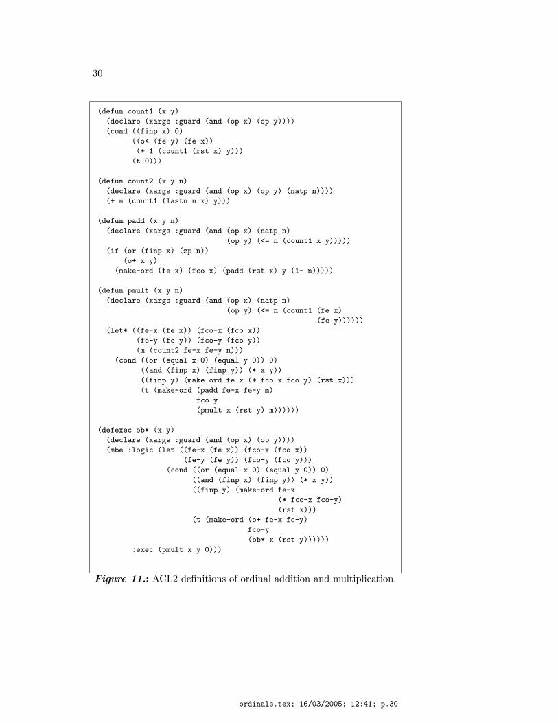
An example of ACL2 definitions appears in Figure 11, where we giveour definition of ordinal multiplication (ob*). Functions are definedwith the defun construct, e.g., consider the definition of count1. Thefirst argument, in this case, count1, is the name of the function. Thesecond argument is a list of its parameters. The last argument is thebody of the function. Once ACL2 admits the function, an axiom isadded stating that (count1 x y) is equal to the body of count1. Thebody of count1 refers to several functions not defined in Figure 11,e.g., finp is the predicate that recognizes if an ordinal is finite andcorresponds to finp from the first part of the paper. The functions fe,fco (not used in count1), and rst correspond to the fe, fco, and rst

functions, respectively. The op function in the declaration correspondsto op.

The declare statement in between the parameters and body ofcount1 is an optional argument that does not affect the meaning of thedefun, but allows the user to inform ACL2 about various pragmaticissues. In this case, we declare the expected type of the inputs, using aguard declaration. Guards are used by the compiler to generate efficientcode. A guard can be any predicate over the function parameters; inthe case of count1, we require that both arguments are ordinals. Whenverifying the guards of a function, ACL2 must demonstrate that whenthe guards conditions for the function hold, the guard conditions forall functions called within the body also hold. For example, we mustprove that whenever count2 calls count1, (lastn n x) and y are bothordinals. If a top level expressions satisfies its guards, then we areguaranteed that no guard violations can occur during execution, andACL2 is free to execute the efficient version of the definition.

Another notable feature of ACL2 is defexec, which the definitionof ob* takes advantage of. Using defexec the user can specify twodefinitions of a function: the :logic definition and the :exec definition.ACL2 is then required to prove that these two definitions are equivalentwhen the guards hold, which allows ACL2 to use the simpler :logic

definition when performing symbolic manipulation, but to use the moreefficient :exec definition during execution. In our case, we use the

ordinals.tex; 16/03/2005; 12:41; p.29

30

(defun count1 (x y)

(declare (xargs :guard (and (op x) (op y))))

(cond ((finp x) 0)

((o< (fe y) (fe x))

(+ 1 (count1 (rst x) y)))

(t 0)))

(defun count2 (x y n)

(declare (xargs :guard (and (op x) (op y) (natp n))))

(+ n (count1 (lastn n x) y)))

(defun padd (x y n)

(declare (xargs :guard (and (op x) (natp n)

(op y) (<= n (count1 x y)))))

(if (or (finp x) (zp n))

(o+ x y)

(make-ord (fe x) (fco x) (padd (rst x) y (1- n)))))

(defun pmult (x y n)

(declare (xargs :guard (and (op x) (natp n)

(op y) (<= n (count1 (fe x)

(fe y))))))

(let* ((fe-x (fe x)) (fco-x (fco x))

(fe-y (fe y)) (fco-y (fco y))

(m (count2 fe-x fe-y n)))

(cond ((or (equal x 0) (equal y 0)) 0)

((and (finp x) (finp y)) (* x y))

((finp y) (make-ord fe-x (* fco-x fco-y) (rst x)))

(t (make-ord (padd fe-x fe-y m)

fco-y

(pmult x (rst y) m))))))

(defexec ob* (x y)

(declare (xargs :guard (and (op x) (op y))))

(mbe :logic (let ((fe-x (fe x)) (fco-x (fco x))

(fe-y (fe y)) (fco-y (fco y)))

(cond ((or (equal x 0) (equal y 0)) 0)

((and (finp x) (finp y)) (* x y))

((finp y) (make-ord fe-x

(* fco-x fco-y)

(rst x)))

(t (make-ord (o+ fe-x fe-y)

fco-y

(ob* x (rst y))))))

:exec (pmult x y 0)))

Figure 11.: ACL2 definitions of ordinal addition and multiplication.

ordinals.tex; 16/03/2005; 12:41; p.30

Ordinal Arithmetic: Algorithms and Mechanization 31

inefficient version of multiplication (given in Section 6) for the :logic

definition and the efficient version for the :exec definition. We also usedefexec to define ordinal exponentiation.

8.2. Mechanical Verification

The mechanical verification of the ordinal arithmetic algorithm imple-mentations involved proving two different classes of theorems, beyondthe guard conjectures and termination proofs mentioned in the previoussection. The first class deals with the algebraic properties of the opera-tions. We proved that each function has the same algebraic propertiesas its corresponding set-theoretic operation. For example, we provedthat ob+, ob-, ob*, and ob^ have all the properties we listed for ordinaladdition, subtraction, multiplication, and exponentiation in Section 2.

The second class of theorems are about the notation and involvehelper functions, such as make-ord, fe, fco, and rst, and how theyinteract with the algebraic functions. An example of this is the followingtheorem.

(defthm o+-fe-1

(implies (o< (fe a)

(fe b))

(equal (fe (o+ a b))

(fe b))))

Recall that all of these theorems are part of the ACL2 distribution.Also, note that these theorems deal with ordinal notations and theimplementations in ACL2 of the ordinal arithmetic algorithms. That is,we do not mechanically establish any connection with the set-theoreticdefinitions on which our algorithms are based, as our goal was notto formalize set-theory in ACL2. Instead, we focused on using ourresults about arithmetic on ordinal notations to extend ACL2’s abilityto reason about termination. However, many of the paper and pencilproofs in the first part of this paper turned out to be quite useful, asthey provided the key insights required to complete the ACL2 proofs.

8.3. Library for Automatic Verification

Enabling ACL2 to effectively and automatically reason about the ordi-nals and termination requires more than proving the correctness of theimplementations, the topic of the previous section. It requires carefullyconstructing a library that makes effective and efficient use of thevarious types of mechanisms that ACL2 provides to control the wayin which theorems are used. A complete description of the issues isbeyond the scope of this paper, but see [38]. Instead, we discuss a fewimportant considerations that went into engineering a useful library.

ordinals.tex; 16/03/2005; 12:41; p.31

32

The first consideration involves a concept in ACL2 known as “ruleclasses.” When ACL2 proves a theorem, it gets entered into a databaseso that it can be used in subsequent proof attempts. By default, theo-rems are entered as rewrite rules. Rewrite rules can be conditional andare triggered when a goal contains an expression matching the left handsize of the rule’s consequent. When this happens, ACL2 attempts toestablish the antecedents of the rule via backchaining, and if successful,it rewrites the expression, using the right hand side of the rewrite rule.For example, consider the following rule.

(defthm |∼(a=0) /\ b>1 <=> a < ab|

(implies (and (op a)

(op b))

(equal (o< a (o* a b))

(and (not (equal a 0))

(not (equal b 0))

(not (equal b 1))))))

After proving this theorem, ACL2 enters it into the database of rulesas a rewrite rule. Subsequently, when ACL2 sees an expression of theform (o< e1 (o* e1 e2)), where e1 and e2 are arbitrary ACL2 ex-pressions, it will try to determine if e1 and e2 are ops. If so, ACL2will rewrite (o< e1 (o* e1 e2)) to (and (not (equal e1 0)) (not

(equal e2 0)) (not (equal e2 1))). Notice that although (o< e1

(o* e1 e2)) is smaller in size than (and (not (equal e1 0)) (not

(equal e2 0)) (not (equal e2 1))), it contains o< and o*, whichare relatively complex functions. It is important to orient rewrite rulesso that they reduce expressions containing complex functions into ex-pressions containing simpler functions. It is also important to take intoaccount how much effort will be expended trying to discharge the hy-potheses, and rules should be written in a way that forces expressionsinto “canonical” forms.

While rewrite rules are the most widely used rule class, there areother types of rules, e.g., forward chaining rules are triggered whenall of the antecedents are known to be true. When this happens, theconsequent is added to the “context,” the collection of known facts.When dealing with large libraries such as ours, the interaction betweenrules of different classes can become quite complicated and the decisionsmade about which rules to put in which classes therefore has a signifi-cant impact on the effectiveness and efficiency of a library of theorems.There are general guidelines as to which rule classes to use [27, 26], butengineering an efficient library requires a good dose of experimentationand profiling.

It is also important to distinguish between the theorems that onewants to export versus the intermediate lemmas that are used to prove

ordinals.tex; 16/03/2005; 12:41; p.32

Ordinal Arithmetic: Algorithms and Mechanization 33

such theorems. For example, to prove the left distributive property ofmultiplication over addition, we had to prove several lemmas whichcorrespond to special cases of the theorem. The distributive propertytheorem should be exported (made visible when the library is loadedinto ACL2), but the supporting lemmas should not. This is accom-plished with ACL2’s local form. Sometimes a lemma can also causeproblems within a library and in this case, one can use the encapsulateform, which provides a way of hiding local theorems from the rest ofthe library (and much more).

Another concern is deciding when to use macros and when to usefunctions. In ACL2 macros are simply syntactic sugar and are expandedaway before theorem proving begins. Thus, ACL2 does not reason aboutmacros. In designing our library, we used macros in two ways. The firstwas to simplify the class of theorems needed to reason about the ordi-nals. For example, we made o<= a macro such that (o<= a b) expandsto (not (o< b a)). This greatly simplified our library, because we didnot need to develop rewrite rules to reason about expressions involvingo<=. The problem with this approach is that the output generated byACL2 is with respect to o<, so we altered ACL2 to print (o<= a b)

instead of (not (o< b a)). This leads to improved readability.The second way we used macros was to create polyadic versions

of our binary functions. For example, o* is a macro and (o* x y z)

macro expands to (ob* x (ob* y z)). We also include similar macrosfor addition and exponentiation. To improve readability, ACL2 can beinstructed to print ob* in terms of o* with the command (add-binop

o* ob*). Thus, users are under the illusion that they are reasoningabout polyadic functions, while all reasoning is really with respect tothe binary functions. In summary, macros provide not only syntacticextensions, but also provide limited support for maintaining the illusionthat users can reason about these extensions, thereby simplifying theinterface between theorem prover and user.

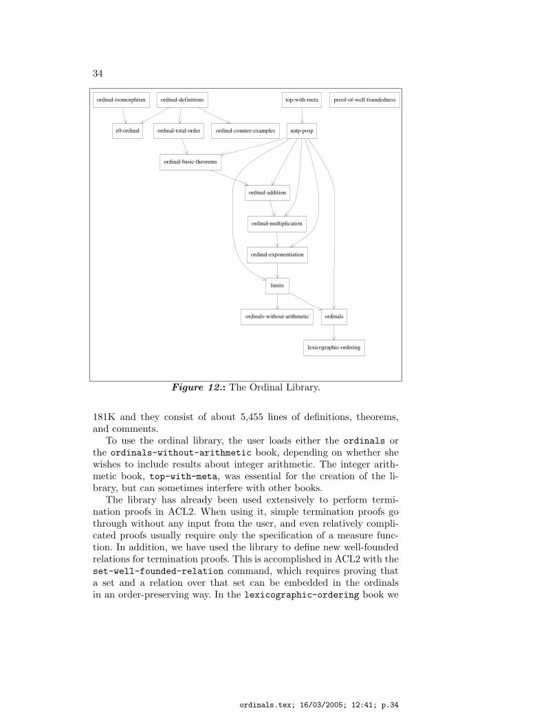
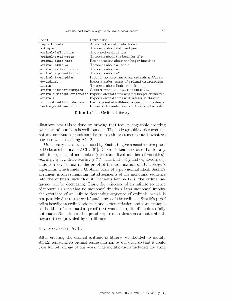
The final consideration we address here is the structure of the library.The library is divided into files of ACL2 theorems and definitions, called“books.” Dividing the theorems properly between the books adds logi-cal coherence and modularity to the library. This maximizes efficiencythrough code reuse and makes the books easier to understand for users.The structure of this library is illustrated in Figure 12, where therectangles represent books, and the arrows represent the dependenciesbetween books. For example, the arrow from ordinal-isomorphism

to e0-ordinal indicates that the results of e0-ordinal rely on theresults of ordinal-isomorphism. A short description of the contentsof the books can be found in Table I. The total size of the books is

ordinals.tex; 16/03/2005; 12:41; p.33

34

e0-ordinal

ordinal-exponentiation

lexicographic-ordering

ordinal-isomorphism

limits

ordinal-multiplication

natp-pospordinal-total-order

ordinals-without-arithmetic

proof-of-well-foundedness

ordinals

top-with-meta

ordinal-basic-theorems

ordinal-addition

ordinal-counter-examples

ordinal-definitions

Figure 12.: The Ordinal Library.

181K and they consist of about 5,455 lines of definitions, theorems,and comments.

To use the ordinal library, the user loads either the ordinals orthe ordinals-without-arithmetic book, depending on whether shewishes to include results about integer arithmetic. The integer arith-metic book, top-with-meta, was essential for the creation of the li-brary, but can sometimes interfere with other books.

The library has already been used extensively to perform termi-nation proofs in ACL2. When using it, simple termination proofs gothrough without any input from the user, and even relatively compli-cated proofs usually require only the specification of a measure func-tion. In addition, we have used the library to define new well-foundedrelations for termination proofs. This is accomplished in ACL2 with theset-well-founded-relation command, which requires proving thata set and a relation over that set can be embedded in the ordinalsin an order-preserving way. In the lexicographic-ordering book we

ordinals.tex; 16/03/2005; 12:41; p.34

Ordinal Arithmetic: Algorithms and Mechanization 35

Book Description

top-with-meta A link to the arithmetic booksnatp-posp Theorems about natp and pospordinal-definitions The function definitionsordinal-total-order Theorems about the behavior of o<ordinal-basic-thms Basic theorems about the helper functionsordinal-addition Theorems about o+ and o-

ordinal-multiplication Theorems about o*

ordinal-exponentiation Theorems about o^

ordinal-isomorphism Proof of isomorphism of our ordinals & ACL2’se0-ordinal Exports major results of ordinal-isomorphismlimits Theorems about limit ordinalsordinal-counter-examples Counter-examples, e.g., commutativityordinals-without-arithmetic Exports ordinal thms without integer arithmeticordinals Exports ordinal thms with integer arithmeticproof-of-well-foundedness Part of proof of well-foundedness of our ordinalslexicographic-ordering Proves well-foundedness of a lexicographic order

Table I.: The Ordinal Library.

illustrate how this is done by proving that the lexicographic orderingover natural numbers is well-founded. The lexicographic order over thenatural numbers is much simpler to explain to students and is what wenow use when teaching ACL2.

Our library has also been used by Sustik to give a constructive proofof Dickson’s Lemma in ACL2 [61]. Dickson’s Lemma states that for anyinfinite sequence of monomials (over some fixed number of variables),m0, m1, m2, . . ., there exists i, j ∈ N such that i < j and mi divides mj .This is a key lemma in the proof of the termination of Buchberger’salgorithm, which finds a Grobner basis of a polynomial ideal. Sustik’sargument involves mapping initial segments of the monomial sequenceinto the ordinals such that if Dickson’s lemma fails, the ordinal se-quence will be decreasing. Thus, the existence of an infinite sequenceof monomials such that no monomial divides a later monomial impliesthe existence of an infinite decreasing sequence of ordinals, which isnot possible due to the well-foundedness of the ordinals. Sustik’s proofrelies heavily on ordinal addition and exponentiation and is an exampleof the kind of termination proof that would be quite difficult to fullyautomate. Nonetheless, his proof requires no theorems about ordinalsbeyond those provided by our library.

8.4. Modifying ACL2

After creating the ordinal arithmetic library, we decided to modifyACL2, replacing its ordinal representation by our own, so that it couldtake full advantage of our work. The modifications included updating

ordinals.tex; 16/03/2005; 12:41; p.35

36

the documentation and modifying the ACL2 sources and consistedof about 1,750 lines of code and documentation. We submitted thechanges to Kaufmann and Moore, the authors of ACL2, and they haveincorporated the changes into the ACL2 version 2.8 [27].

It is worth noting that our changes do not affect the soundness ofthe ACL2 logic. In the ordinal-isomorphism book of our library, weexhibit a bijection between our ordinal representation and the previousACL2 representation (see Corollary 1). This proof was carried out inACL2 version 2.7, thus guaranteeing that soundness is not affected.

We now discuss some of the issues we confronted in modifying ACL2.First, the ordinals are needed in ACL2’s ground-zero theory, the initialtheory encountered when starting an ACL2 session. Proving theorems,defining functions, including books, etc. all result in extensions to theground-zero theory, and we wanted to keep it as clean and simple aspossible. Therefore, we did not want to add our entire library of defi-nitions and theorems to the ground-zero theory. Instead, we includedonly the basic constructors and destructors (make-ord, fe, fco, rst),the functions necessary for op and o< (natp, posp, infp, finp, o<, op),and a few macros based on o< (o>, o<=, o>=). The arithmetic functionsand theorems remain in the library.

After replacing the old ordinals with our new representation, wehad to deal with legacy issues, including backward compatibility forthe books included with ACL2, as many of these books referenced theold ordinal representation. The key to fixing these references was thetheorems proved in the ordinal-isomorphism and e0-ordinal books.The main result in the books is a proof that there exists a bijectionbetween the new and old ordinal representations. This result allowedus to switch the well-founded relation used by ACL2 to the version2.7 relation (for the admission of the troublesome books only). Thatfixed most of the problems, however, some books used the old ordinalsto prove more than just termination. Again, by using the bijectionproof, we were able to transfer results about the old ordinals to thenew ordinals, which resolved the remaining problems.

9. Conclusion

We presented efficient algorithms for ordinal addition, subtraction,multiplication, and exponentiation on succinct ordinal representations,proved their correctness, and analyzed their complexity. We imple-mented the algorithms in the ACL2 system, mechanically verified thecorrectness of the implementations, and developed a library of theoremsthat can be used to significantly automate reasoning involving the ordi-

ordinals.tex; 16/03/2005; 12:41; p.36

Ordinal Arithmetic: Algorithms and Mechanization 37

nals. We modified ACL2 so that it directly supports our representationof the ordinals and our libraries; the modifications are part of ACL2version 2.8. While the theory of the ordinal numbers has been studiedby various research communities for over 100 years, we believe thatwe are the first to give algorithms for ordinal arithmetic on ordinalnotations.

Our work can be extended by replacing ε0 with larger countableordinals. A simple counting argument shows that no ordinal notationcan represent all countable ordinals, but there are well known notationsthat can represent ordinals up to Γ0 (which is needed to show termina-tion of some term rewrite systems [15, 20]) and further into the Veblenhierarchies [65] and further still [40, 58, 59]. Another possible extensionis to define additional operations on ordinals, e.g., division, taking logs,etc. Finally, a promising direction for future work is to use our libraryand ACL2 as a proof checker for termination tools that guess measurefunctions in some heuristic fashion and to apply these tools to systemswritten in common imperative languages such as C and Java.

AcknowledgmentsWe would like to thank Matt Kaufmann and J Strother Moore forintegrating our modifications into ACL2 version 2.8. We would alsolike to thank Matyas Sustik for using our library and making manysuggestions on how we can improve it.

References

1. K. R. Apt and E.-R. Olderog. Verification of Sequential and ConcurrentPrograms. Springer-Verlag, New York, 1991.

2. F. Baader and T. Nipkow. Term Rewriting and All That. Cambridge UniversityPress, 1998.

3. G. Bancerek. The reflection theorem. Journal of Formalized Mathematics, 2,1990. See URL http://megrez.mizar.org/mirror/JFM/Vol2/zf refle.html.

4. J. G. Belinfante. Computer proofs in Godel’s class theory with equa-tional definitions for composite and cross. Journal of Automated Reasoning,22(3):311–339, 1999.

5. J. G. F. Belinfante. On computer-assisted proofs in ordinal number theory.Journal of Automated Reasoning, 22(3):341–378, 1999.

6. J. G. F. Belinfante. Reasoning about iteration in Godel’s class theory. InF. Baader, editor, Automated Deduction - CADE-19, Proceedings of the 19thInternational Conference on Automated Deduction, volume 2741 of LNAI,pages 228–242. Springer-Verlag, 2003.

7. Y. Bertot and P. Casteran. Interactive Theorem Proving and Program Devel-opment, Coq’Art: the calculus of inductive constructions. Texts in TheoreticalComputer Science. Springer-Verlag, May 2004.

8. R. S. Boyer and J. S. Moore. A Computational Logic Handbook. AcademicPress, second edition, 1997.

ordinals.tex; 16/03/2005; 12:41; p.37

38

9. B. Brock, M. Kaufmann, and J. S. Moore. ACL2 theorems about commercialmicroprocessors. In M. Srivas and A. Camilleri, editors, Formal Methods inComputer-Aided Design (FMCAD’96), pages 275–293. Springer-Verlag, 1996.

10. G. Cantor. Beitrage zur Begrundung der transfiniten Mengenlehre. Mathema-tische Annalen, xlvi:481–512, 1895.

11. G. Cantor. Beitrage zur Bgrundung der transfiniten Mengenlehre. Mathema-tische Annalen, xlix:207–246, 1897.

12. G. Cantor. Contributions to the Founding of the Theory of Transfinite Numbers.Dover Publications, Inc., 1952. Translated by Philip E. B. Jourdain.

13. A. Church and S. C. Kleene. Formal definitions in the theory of ordinalnumbers. Fundamenta mathematicae, 28:11–21, 1937.

14. L. A. Dennis and A. Smaill. Ordinal arithmetic: A case study for rippling in ahigher order domain. In R. Boulton and P. Jackson, editors, Theorem Provingin Higher Order Logics: 14th International Conference, TPHOLs 2001, volume2152 of LNCS, pages 185–200. Springer-Verlag, 2001.

15. N. Dershowitz and M. Okada. Proof-theoritic techniques for term rewritingtheory. In 3rd IEEE Symp. on Logic in Computer Science, pages 104–111,1988.

16. N. Dershowitz and E. M. Reingold. Ordinal arithmetic with list structures. InLogical Foundations of Computer Science, pages 117–126, 1992.

17. K. Devlin. The Joy of Sets: Fundamentals of Contemporary Set Theory.Springer-Verlag, second edition, 1992.

18. J. Doner. Definability in the extended arithmetic of ordinal numbers.Dissertationes Mathematicae, 96, 1972.

19. J. Doner and A. Tarski. An extended arithmetic of ordinal numbers.Fundamenta Mathematicae, 65:95–127, 1969.

20. J. H. Gallier. What’s so special about Kruskal’s theorem and the ordinal Γ0?A survey of some results in proof theory. Annals of Pure and Applied Logic,pages 199–260, 1991.

21. G. Gentzen. Die Widerspruchsfreiheit der reinen Zahlentheorie. MathematischeAnnalen, 112:493–565, 1936. English translation in M. E. Szabo (ed.), TheCollected Works of Gerhard Gentzen, pp. 132-213, North Holland, Amsterdam,1969.

22. M. J. C. Gordon and T. F. Melham, editors. Introduction to HOL: A TheoremProving Environment for Higher Order Logic. Cambridge University Press,1993.

23. D. Greve, M. Wilding, and D. Hardin. High-speed, analyzable simulators. InKaufmann et al. [25], pages 113–135.

24. D. A. Greve. Symbolic simulation of the JEM1 microprocessor. In FormalMethods in Computer-Aided Design – FMCAD, LNCS. Springer-Verlag, 1998.

25. M. Kaufmann, P. Manolios, and J. S. Moore, editors. Computer-AidedReasoning: ACL2 Case Studies. Kluwer Academic Publishers, June 2000.

26. M. Kaufmann, P. Manolios, and J. S. Moore. Computer-Aided Reasoning: AnApproach. Kluwer Academic Publishers, July 2000.

27. M. Kaufmann and J. S. Moore. ACL2 homepage. See URL http://www.cs.-

utexas.edu/users/moore/acl2.28. M. Kaufmann and J. S. Moore, editors. Proceedings of the ACL2 Work-

shop 2000. The University of Texas at Austin, Technical Report TR-00-29,November 2000.

ordinals.tex; 16/03/2005; 12:41; p.38

Ordinal Arithmetic: Algorithms and Mechanization 39

29. M. Kaufmann and J. S. Moore, editors. Fourth International Workshop on theACL2 Theorem Prover and Its Applications (ACL2-2003), July 2003. See URLhttp://www.cs.utexas.edu/users/moore/acl2/workshop-2003/.

30. K. Kunen. Set Theory - An Introduction to Independence Proofs, volume102 of Studies in Logic and the Foundations of Mathematics. North-Holland,Amsterdam, 1980.

31. P. Manolios. Correctness of pipelined machines. In W. A. Hunt, Jr. and S. D.Johnson, editors, Formal Methods in Computer-Aided Design–FMCAD 2000,volume 1954 of LNCS, pages 161–178. Springer-Verlag, 2000.

32. P. Manolios. Mechanical Verification of Reactive Systems. PhD thesis,University of Texas at Austin, August 2001. See URL http://www.cc.-

gatech.edu/∼manolios/publications.html.33. P. Manolios and J. S. Moore. Partial functions in ACL2. In Kaufmann and

Moore [28].34. P. Manolios and J. S. Moore. Partial functions in ACL2. Journal of Automated

Reasoning, 31(2):107–127, 2003.35. P. Manolios, K. Namjoshi, and R. Sumners. Linking theorem proving and

model-checking with well-founded bisimulation. In N. Halbwachs and D. Peled,editors, Computer-Aided Verification–CAV ’99, volume 1633 of LNCS, pages369–379. Springer-Verlag, 1999.

36. P. Manolios and D. Vroon. Algorithms for ordinal arithmetic. In F. Baader,editor, 19th International Conference on Automated Deduction – CADE-19,volume 2741 of LNAI, pages 243–257. Springer–Verlag, July/August 2003.

37. P. Manolios and D. Vroon. Ordinal arithmetic in ACL2. In Kaufmannand Moore [29]. See URL http://www.cs.utexas.edu/users/moore/acl2/-

workshop-2003/.38. P. Manolios and D. Vroon. Integrating reasoning about ordinal arithmetic

into ACL2. In Formal Methods in Computer-Aided Design: 5th InternationalConference – FMCAD-2004, LNCS. Springer–Verlag, November 2004.

39. I. Medina-Bulo, F. Palomo-Lozano, and J. A. Alonso-Jimenez. Implementationin ACL2 of well-founded polynomial orderings. In M. Kaufmann and J. S.Moore, editors, Proceedings of the ACL2 Workshop 2002. 2002.

40. L. W. Miller. Normal functions and constructive ordinal notations. Journal ofSymbolic Logic, 41:439–459, June 1976.

41. J. S. Moore, T. Lynch, and M. Kaufmann. A mechanically checked proof of theAMD5K86 floating-point division program. IEEE Trans. Comp., 47(9):913–926, September 1998.

42. F. Morris and C. Jones. An early program proof by Alan Turing. IEEE Annalsof the History of Computing, 6(2):139–143, April–June 1984.

43. S. Owre, J. Rushby, and N. Shankar. PVS: A prototype verification system.In D. Kapur, editor, 11th International Conference on Automated Deduction(CADE), pages 748–752. Lecture Notes in Artificial Intelligence, Vol 607,Springer-Verlag, June 1992.

44. L. C. Paulson. Set theory for verification: I. From foundations to functions.Journal of Automated Reasoning, 11(3):353–389, 1993.

45. L. C. Paulson. Isabelle: A Generic Theorem Prover. Springer-Verlag LNCS828, 1994.

46. L. C. Paulson. Set theory for verification: II. Induction and recursion. Journalof Automated Reasoning, 15(2):167–215, 1995.

ordinals.tex; 16/03/2005; 12:41; p.39

40

47. L. C. Paulson. The reflection theorem: a study in meta-theoretic reasoning.In A. Voronkov, editor, 18th International Conf. on Automated Deduction:CADE-18, number 2392 in LNAI, pages 377–391. Springer-Verlag, 2002.

48. L. C. Paulson. The relative consistency of the axiom of choice mechanized usingisabelle. LMS Journal of Computation and Mathematics, 6:198–248, 2003.

49. L. C. Paulson and K. Grabczewski. Mechanizing set theory: cardinal arithmeticand the axiom of choice. Journal of Automated Reasoning, 17:291–323, 1996.

50. H. Rogers, Jr. Theory of Recursive Functions and Effective Computability.MIT Press, 1st paperback edition, 1987.

51. P. Rudnicki. An overview of the MIZAR project. In 1992 Workshop on Typesfor Proofs and Programs, 1992.

52. J.-L. Ruiz-Reina, J.-A. Alonso, M.-J. Hidalgo, and F.-J. Martin. Multisetrelations: A tool for proving termination. In Kaufmann and Moore [28].

53. D. M. Russinoff. A mechanically checked proof of correctness of the AMD5K86floating-point square root microcode. Formal Methods in System Design SpecialIssue on Arithmetic Circuits, 1997.

54. D. M. Russinoff. A mechanically checked proof of IEEE compliance of aregister-transfer-level specification of the AMD-K7 floating-point multiplica-tion, division, and square root instructions. London Mathematical SocietyJournal of Computation and Mathematics, 1:148–200, December 1998.

55. D. M. Russinoff. A mechanically checked proof of correctness of the AMD-K5 floating-point square root microcode. Formal Methods in System Design,14:75–125, 1999.

56. D. M. Russinoff and A. Flatau. RTL verification: A floating-point multiplier.In Kaufmann et al. [25], pages 201–231.

57. K. Schutte. Proof Theory. Springer-Verlag, 1977. Translation from the Germanby J. N. Crossley. The book is a completely rewritten version of Beweistheorie,Springer-Verlag, 1960.

58. A. Setzer. Ordinal systems. In B. Cooper and J. Truss, editors, Sets and Proofs,pages 301–331. Cambridge University Press, 1999.

59. A. Setzer. Ordinal systems part 2: One inaccessible. In Logic Colloquium ’98,volume 13 of ASL Lecture Notes in Logic, pages 426–448, 2000.

60. R. Sumners. An incremental stuttering refinement proof of a concurrentprogram in ACL2. In Kaufmann and Moore [28].

61. M. Sustik. Proof of Dixon’s lemma using the ACL2 theorem prover via anexplicit ordinal mapping. In Kaufmann and Moore [29]. See URL http://-

www.cs.utexas.edu/users/moore/acl2/workshop-2003/.62. A. S. Troelstra and H. Schwichtenberg. Basic Proof Theory. Cambridge

University Press, second edition, 2000.63. A. M. Turing. Systems of logic based on ordinals. Proceedings of the

London Mathematical Society, 45(2):161–228, 1939. See URL http://www.-

turingarchive.org/.64. A. M. Turing. Checking a large routine. In Report of a Conference on High

Speed Automatic Calculating Machines, pages 67–69. Universtity MathematicalLaboratory, Cambridge, June 1949.

65. O. Veblen. Continuous increasing functions of finite and transfinite ordinals.Transactions of the American Mathematical Society, 9:280–292, 1908.

ordinals.tex; 16/03/2005; 12:41; p.40