OrdinaryDifferentialEquations andIntroductiontoDynamical ... · PDF fileOrdinaryDifferentialEquations andIntroductiontoDynamical Systems ... Consider the dynamical system, ... differential

Ordinary Differential Equationsand Introduction to Dynamical

SystemsHolly D. Gaff

[email protected]

University of Tennessee, Knoxville

SMB Short Course 2002 – p.1/57

Overview

� Single Species Systems� Solving for Equilibria� Evaluating Stability of EquilibriaGraphically� Two Species Systems� Lotka-Volterra Predator-Prey� Evaluating Stability of Equilibria� Examples from Epidemiology


Single Species Systems

� Exponential Growth� Logistic Growth� Other Equations


Exponential Growth

��

Solution: � � � � � �What happens to this population?


Exponential Growth

Exponential Growth

0

10000

20000

30000

40000

50000

60000

70000

N(t)

2 4 6 8 10

t


Logistic Growth

��

What do you think the solutions of this will looklike?Recall exponential growth was�

� � �


Equilibria

��

��

� � � � � � �

� � � � � � �


Stability of EquilibriaFirst evaluate the stability of

� � �.

Near

� � �

,

�� !

So as increase,

"# "$ grows exponentially.

Therefore,

� � �is an unstable equilibrium.


Stability of EquilibriaWhat do you think will happen near

% & ?

''( & ) * +


Stability nearIf is just slightly above ,

,,- . / 0 1 2 3

but if is just slightly below ,

,,- . / 0 1 4 3

Therefore,

5 . is stable.


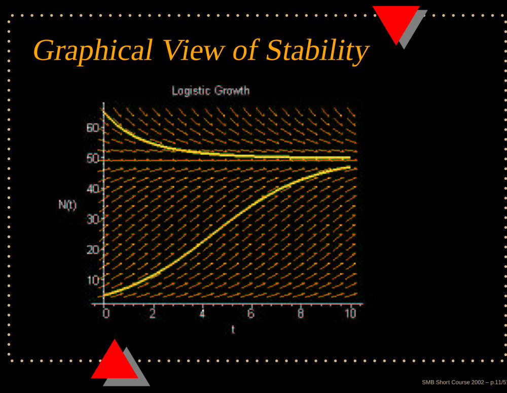
Graphical View of Stability


Other Alternatives

6 Gompertz Equation778 9 :<; = > ? @

6 Delay or lag time778 9 A A 8 BC A 8 D B B


Other Alternatives

E Allee effectFFG H I J K L K J

E Discrete time M G J N H M M G N N

E Stochastic processes


Interacting Populations

O Predator-prey models

O Competition

O Mutualism


Classic Predator-Prey

Lotka-Volterra Predator-Prey ModelPPQ R S T U

PPQ R V T W


Classic Predator-Prey

Lotka-Volterra Predator-Prey ModelX Historical interestX Mass-action termX Bad mathematical modelX Structurally unstable


Lotka-Volterra Phase Plane


Interacting PopulationsMore Realistic Predator-prey models

YYZ [ \ ]_^ ^

YYZ [ ` ^ Y


Interacting PopulationsAnother More Realistic Predator-prey models

aab c d e_f f g g

aab c h g g f a


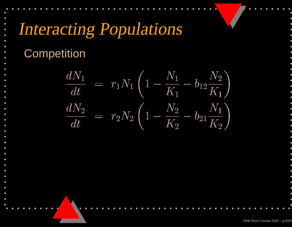
Interacting PopulationsCompetition

i jik l m j j n_o jj o p jq qji qik l mq q n_o q

q o pq j jq


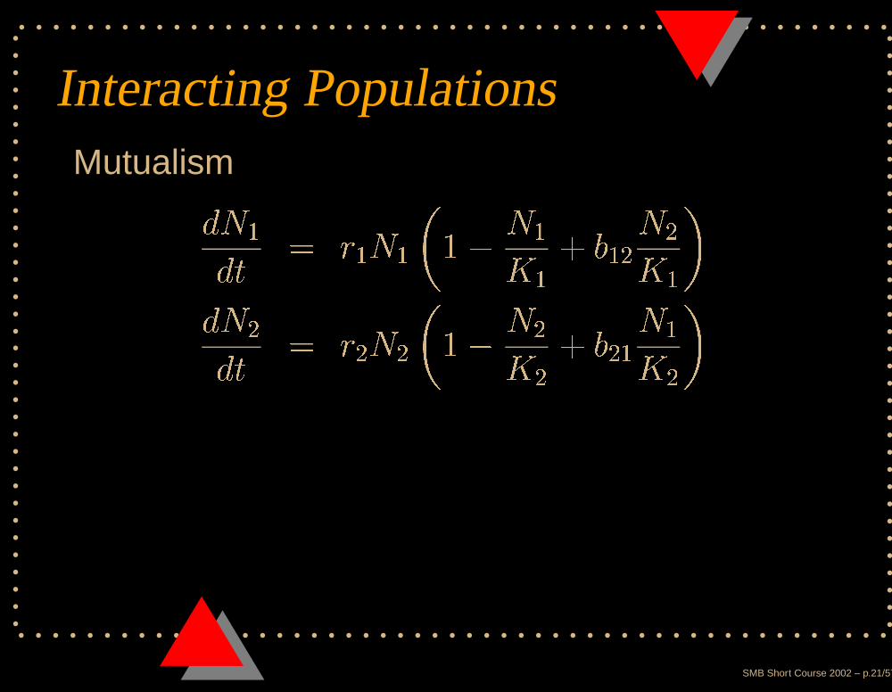
Interacting PopulationsMutualismr srt u v s s w_x s

s y sz zsr zrt u vz z w_x z

z yz s sz


Interacting PopulationsTo analyze these types of models{ Nondimensionalize the system{ reduce the number of parameters{ simplfy the system{ Solve for equilibria{ Analyze stability of equilibria{ Translate back to determine biological

significance


Phase-Plane TechniquesSome defintions of stability| Stable - if start small distance from

equilibrium, remain small distance as

}

| Lyapunov stable| locally stable| Asymptotically stable - if start small distancefrom equilibrium, distance from equilibriumapproaches zero as

}

| locally asymptotically stable


Phase-Plane Techniques

~ Linearization~ Bendixson-Dulac negative criterion~ Hopf bifurcation theorem~ Poincaré-Bendixson theorem~ Routh-Hurwitz Conditions


LinearizationGiven: �

��

��


LinearizationSolve: � ��

� �� to find the equilibria,

� �� .

Let:

� ��

� ��


LinearizationThen linearize about the equilibrium:

��

��

��

� ��

��

��

Or:

� � � ¡<¢ ¢ ¡¢£¡£ ¢ ¡£ £

��


LinearizationLet:

¤ ¥ ¦<§ § ¦<§¨¦¨ § ¦¨ ¨

Where

¤

is known as the Jacobian matrix or thecommunity matrix.We now look for solutions of the form:

© ª�« ¬ ¥ ©< ® ¯°

± ª�« ¬ ¥ ± ® ¯°


LinearizationSubstitute this back into the equations to obtain:

²�³<´ µ ¶<· · ³ ´ ¶<·¸ ¹´² ¹´ µ ¶¸ · ³ ´ ¶¸ ¸ ¹´or

¶�· · º ² ¶ ·¸

¶¸ · ¶¸ ¸ º ² ³�´¹´ µ »


LinearizationFrom this, we obtain the characteristic equation

¼ ½¾ ¿ÁÀ�Â Â À ½ ½ Ã ¼ ¿ÀÂ Â À ½ ½ ¾ ÀÂ ½ À ½Â Ã Ä Å

Solving for the two roots of¼

will determine the

stability of the system.


Linearization

Æ If both roots of

Ç

are real and negative, theequilibrium is a stable node.Æ If both roots of

Ç

are real and positive, theequilibrium is an unstable node.Æ If the roots of

Ç

are real and of opposite signs,the equilibrium is a saddle point.


Linearization

È If the roots of

É

are complex with negativereal parts, the equilibrium is a stable focus.È If the roots of

É

are complex with positive realparts, the equilibrium is an unstable focus.È If the roots of

É

are purely complex, theequilibrium of the linearized system is acenter, but the original nonlinear system willhave a center or a stable or unstable focusdepending upon the exact nature of thenonlinear terms.


Routh-Hurwitz conditionsRouth-Hurwitz conditions give the necessary andsufficient conditions for all roots of thecharacteristic polynomial to have negative realroots thus implying asymptotic stability.

Ê Ë Ì Í Ë Î�Ï Ï Î�Ð Ð Ñ Ò

Ó Ë Ô�Õ Ö Í Ë Î<Ï Ï Î<Ð Ð × Î<Ï Ð Î<Ð Ï Ø Ò


Stability


Bendixson negative criterionBendixson’s negative criterion

Consider the dynamical system,

ÙÛÚ ÙÜ ÝÞÁßáà â ãà ÙÛä ÙÜ Ý Þßáà â ãà where and are contin-

uously differentiable functions on some simply

connected domain å æ. If ç Þ à ã Ý èé è Ú èê è ä

is of one sign in , there cannot be a closed orbit

contained within .


Bendixson-Dulac negative crite-rionAdditionally, we have the Bendixson’s-Dulac’snegative criterion.

Let be a smooth function on ë ì(with above

assumptions). If í î ï ð ñ òó ôòöõ òó ÷òöø is

of one sign in , there cannot be a closed orbit

contained within .


Other theorems

ù The Hopf bifurcation theorem givesconditions necessary for the existence of realperiodic solutions of a real system of ordinarydifferential equations.ù Poincaré-Bendixson theorem can also beused to prove the existence of periodic orbits.


Examples from EpidemiologyDivide population up into distinct classesú û ü Susceptiblesú ý ü Infectivesú ü Recovered

Classes used depend on disease dynamics


SIR Model

S RI

µN

α β

µ µ µS

S I

I

I

R


SIR Model - constant population

þ ÿþ� � � � ÿ � � � � ÿ � � � ÿ

þ �þ� � � ÿ � � � � � �

þþ� � � � �

� ÿ �

ÿ �� ÿ� � � �� All parameters are

assumed to be positive.


Questions for Epidemic Models

Given all parameters and initial conditions

� Does the infection spread or die out?

� If it does spread, how does it develop withtime?

� When will it start to decline?


EquilibriaNote: Since is a constant, we can solve foronly

�

and

�

, then if we need , we can calculateit easily.

� ��

� ��


EquilibriaGives two equilibria:

� � � � � � � �

� � � � � � � � � ! " " � #

! � #

Let

! � � � # � � " � � " � �

! � � � # � � � " � " � �


StabilityThen $

$% & ' ( ) ' *

$$ ) & ' ( %

$$% & ( )

$$ ) & ( % ' ' *


StabilityFirst, let’s evaluate the stability of

+, - . /, - 0

The elements of the Jacobian evaluated at thisequilibrium are:

132 2 - 4 5

1326 - 4 7

16 2 - 0

16 6 - 7 4 4 5


StabilityApplying the Routh-Hurwitz conditions:

8:9 9 8:; ; < = = >@?

89 9 8:; ; = 89 ; 8:; 9 < ? A ? = B C

Clearly, = = >@? D E

However, ? A ? = B C F Eonly if B D ?

Therefore,

GH < I JH < Eis asymptotically stable

if B D ?SMB Short Course 2002 – p.46/57

Disease dies out


StabilityNow, let’s evaluate the stability ofKL M NPO QR S TL M Q U R VXW N W Q YRU NO Q Y

The elements of the Jacobian evaluated at thisequilibrium are:

Z3[ [ M \ ] \ ] ^`_ \ \ ] a] a

Z3[b M \ \ ]

Zb [ M ] ^`_ \ \ ] a] a

Zb b M c


StabilityApplying the Routh-Hurwitz conditions:

dfe e dfg g h i j i j k`l i i j mj m

dfe e dfg g i dfe g dfg e h k j m j k`l i i j mj m


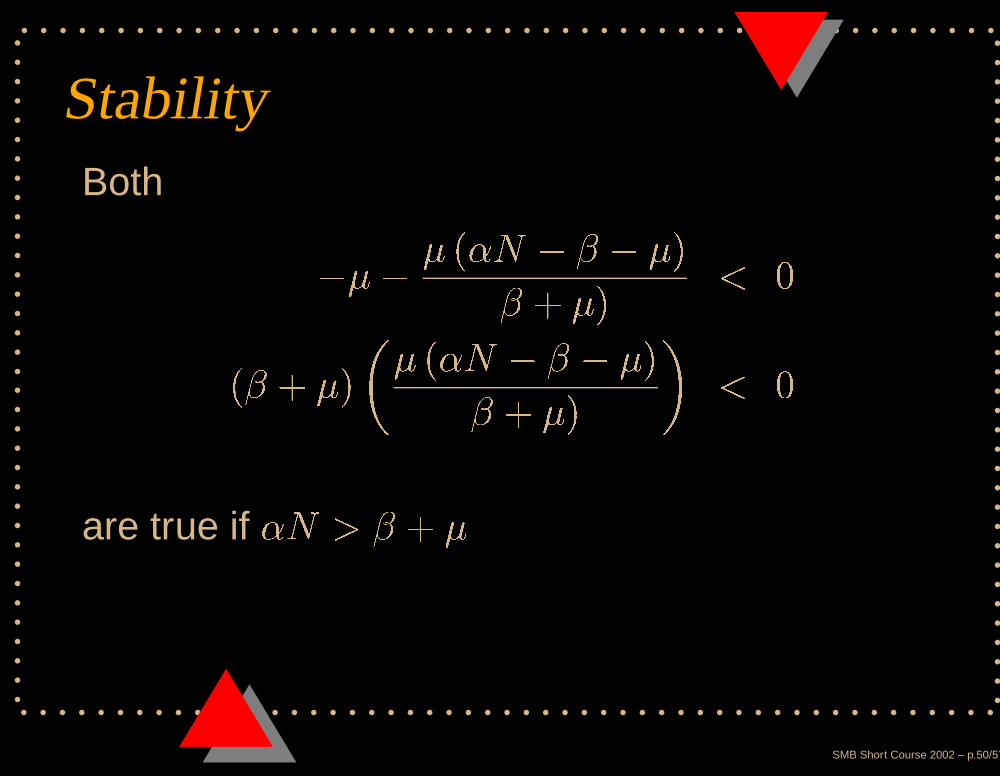
StabilityBoth

n o n o p`q n n o ro r s t

p o r o pq n n o ro r s t

are true if q u o


StabilityTherefore,

vw x yz { | w x y } z ~ ~ y �

z } y �

is asymptotically stable if z � y

But what about limit cycles?


Epidemic


Bendixson’s Negative CriteriaRecall, we need

� � � � � ��

��

to be of one sign in our region of interest, .

Define to be all positive values in

�

.


Bendixson’s Negative Criteria

��

��

So this will be of one sign, negative, if� � � since

�

.

Therefore there are no limit cycles in .


� Basic reproduction rate

� � is defined to be the number of secondaryinfections produced by one primary infectionin a wholly susceptible population.

� So if � � �

, then the disease will spread.

� For SIR model, � is calculated by linearizingthe equation for

�� about

� � �

, which wehave already done.

� So the criteria for determining if the epidemicwill spread is, � � � � �P ¢¡ .


ConclusionsThere are many other applications of differentialequation models in biology. Once a basic set ofequations has been developed, there are anumber of standard techinques used to analyzethe stability of the equations.

We will take time in the lab to explore these and

other equations.


Acknowledgements

£ Murray, J. D., Mathematical Biology,Springer-Verlag, 1989.

£ Kot, Mark, Elements of MathematicalEcology, Cambridge University Press, 2001.

£ Arrowsmith, D.K. and C.M. Place, OrdinaryDifferential Equations, Chapman and Hall,1982.

All slides created in LATEXusing the Prosper class.


Documents

OrdinaryDifferentialEquations andIntroductiontoDynamical ... · PDF fileOrdinaryDifferentialEquations andIntroductiontoDynamical Systems ... Consider the dynamical system, ... differential