ORF 522: Lecture 14

Linear Programming: Chapter 16

Interior-Point Methods

Robert J. Vanderbei

November 7, 2013

Slides last edited at 12:46 Noon on Thursday 7th November, 2013

Operations Research and Financial Engineering, Princeton University

http://www.princeton.edu/∼rvdb

Interior-Point Methods—The Breakthrough

Breakthrough in Problem Solving

"This is a path-breaking result:' said Dr. Ronald L. Graham, director of mathematical sciences for Bell Labs in

By JAMES A?8-year-old mathematician at A.T.m.

Bell Laboratories has made a startling theoretical breakthrough in the solving of systems of equations that often grow too vast and complex for the most powerful computers.

The discovery, which is to be formally published next month, is already cir- culating rapidly through the mathematical world. It has also set off a deluge of inquiries from brokerage houses, oil com- panic$ and airlines, industries with millions of dollars at stake in problems known as linear programming.

Faster Solutions Seen

These problems are fiendishly com- plicated systems, often with thousands of variables. They arise in a variety of com- mid and government applications, rang- ing From allocating time on a communica- tions satellite to routing millions of telephone calls wer long distances, or whenever a limited, expensive resource must be spread most efficiently among wmpeting users. And investment com- panies use them in creating portfolios with the best mix of stocks and bonds.

The Bell Labs mathematician. Dr. Narendra Karmarkar, has devised a radically new pmcedure that may speed the routine handling of such problems by businesses and Government agencies and also make it possible to tackle problems that are now far out of reach.

Murray Hill, N.J. I

GLEICK "Science has its moments of great pro- gress, and this may well be one of them."

Because problems in linear program- ming can have billions or more possible answers, even high-speed computers can- not check every one. So computers must uqe a special procedure, an algorithm, to examine as fnv answers as possible before finding the best one - typically the one that minimizes cost or maximizes efficiency.

A pmcedm devised in 1947, the simplex method, is now used for such problems,

Continued on Page A19, Column 1

THE NEW YORK TIMES, November 19, 1984

Karmarlur a t Ball Labs: an equation to find a new way through the maze

Folding the Perfect Corner A young Bell scientist makes a major math breakthrough

among the fllghC :total of 3 6 million gal should allow cdmputen to track sgrciter <om. of high-octane fuel 1s burned Nuts. bolts, bmation of tasks thm ever before and in a tnc.

very day 1,200 Americen Airlines jets E cr~sscross . the U.S., Mexico. Canada and the Caribbean, stopping in 110 cities and bear- ing cwer 80,000 passengers. More than 4,000 pilots, copilots, flight personnel, maintenance workers and baeeaee carriers are shuffled

altimeters, landing gears and the like must be I tion of the time. checked at each destination. And while per- U n l ~ k e most advances in theoretical

Indian-born mathematician at Bell Laboratories in Murray Hill, N.J.. after only a years' work has cracked the puzzle of linear programming by devising a new algorithm, a step-by-step mathematical formula. He has translated the procedure into a proeranl that

forming these scheduling gymna~tics. t h e I mathematics. K a ~ a r k a r ' s work w ~ l l have an company must kccp a close q e on costs. pro- ~mmcdiate and major impact on the ICA world. jected revenue and profits.

Like American Airlines, thousands of com- panies must routinely untangle the myriad variables that complicate the efficient distribu- tion of their resources. Solving such monstrous problems requires the use of an abstruse branch of mathematics known as linear pro- gramming. It is the kind of math that has fmstratul theoreticians for years, and even the fastest and most powerful computers have had great difficulty juggling the bits and pieces of data. Now Narendra Karmarkar, a 28-year-old

! "Breakthrough is o n e o f the most abused words in science:' says Ronald Graham, d i m - tor of mathematical sciences at Bell Labs. "But this is one situation where it is truly ap- propriate."

8 Before the Kamarkar method. linear equa- 1 tions could be solved only in a cumbersome

fashion, ironically known as the simplex method, devised by Mathematician George Dantzig in 1947. Problems are conceived of as giant geodesic domes with thousands of sides. Each comer of a facet on the dome

TIME MAGAZINE, December 3, 1984

1

The Wall Street Journal Waits ’Till 1986

2

AT&T Patents the Algorithm, Announces KORBX

3

What Makes LP Hard?

Primal

maximize cTxsubject to Ax + w= b

x, w≥ 0

Dual

minimize bTysubject to ATy − z = c

y, z≥ 0

Complementarity Conditions

xjzj = 0 j = 1, 2, . . . , n

wiyi = 0 i = 1, 2, . . . ,m

4

Matrix Notation

The componentwise product of two vectors is called the Hadamard product.

The notation xz is not normally understood as the componentwise product.

We need a notation for the Hadamard product.

Instead, introduce a new notation:

x =

x1

x2...xn

=⇒ X =

x1

x2. . .

xn

Then the complementarity conditions can be written as:

XZe = 0

WY e = 0

5

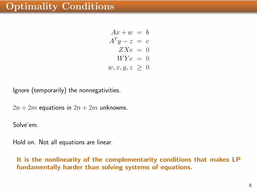
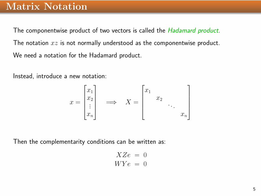
Optimality Conditions

Ax + w = b

ATy − z = c

ZXe = 0

WY e = 0

w, x, y, z ≥ 0

Ignore (temporarily) the nonnegativities.

2n + 2m equations in 2n + 2m unknowns.

Solve’em.

Hold on. Not all equations are linear.

It is the nonlinearity of the complementarity conditions that makes LPfundamentally harder than solving systems of equations.

6

The Interior-Point Paradigm

Since we’re ignoring nonnegativities, it’s best to replace complementarity with µ-complementarity:

Ax + w = b

ATy − z = c

ZXe = µe

WY e = µe

Start with an arbitrary (positive) initial guess: x, y, w, z.

Introduce step directions: ∆x, ∆y, ∆w, ∆z.

Write the above equations for x + ∆x, y + ∆y, w + ∆w, and z + ∆z:

A(x + ∆x) + (w + ∆w) = b

AT (y + ∆y)− (z + ∆z) = c

(Z + ∆Z)(X + ∆X)e = µe

(W + ∆W )(Y + ∆Y )e = µe

7

Paradigm Continued

Rearrange with “delta” variables on left and drop nonlinear terms on left:

A∆x + ∆w = b− Ax− wAT∆y −∆z = c− ATy + z

Z∆x + X∆z = µe− ZXeW∆y + Y∆w = µe−WY e

This is a linear system of 2m + 2n equations in 2m + 2n unknowns.

Solve’em.

Dampen the step lengths, if necessary, to maintain positivity.

Step to a new point:

x ←− x + θ∆x

y ←− y + θ∆y

w ←− w + θ∆w

z ←− z + θ∆z

(θ is the scalar damping factor).

8

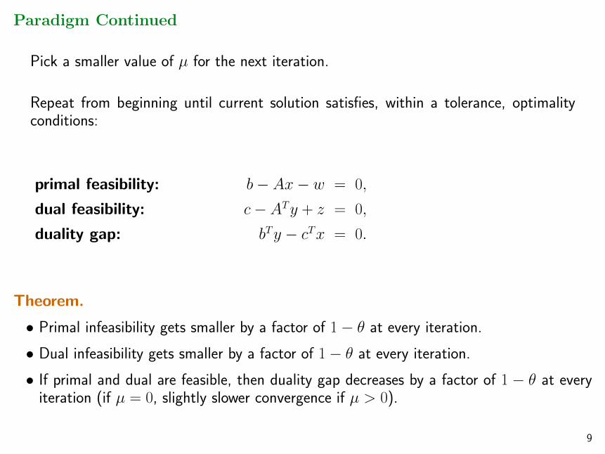
Paradigm Continued

Pick a smaller value of µ for the next iteration.

Repeat from beginning until current solution satisfies, within a tolerance, optimalityconditions:

primal feasibility: b− Ax− w = 0,

dual feasibility: c− ATy + z = 0,

duality gap: bTy − cTx = 0.

Theorem.

• Primal infeasibility gets smaller by a factor of 1− θ at every iteration.

• Dual infeasibility gets smaller by a factor of 1− θ at every iteration.

• If primal and dual are feasible, then duality gap decreases by a factor of 1 − θ at everyiteration (if µ = 0, slightly slower convergence if µ > 0).

9

loqo

Hard/impossible to “do” an interior-point method by hand.

Yet, easy to program on a computer (solving large systems of equations is routine).

LOQO implements an interior-point method.

Setting option loqo options ’verbose=2’ in AMPL produces the following“typical” output:

10

loqo Output

variables: non-neg 1350, free 0, bdd 0, total 1350constraints: eq 146, ineq 0, ranged 0, total 146

nonzeros: A 5288, Q 0

nonzeros: L 7953, arith_ops 101444

---------------------------------------------------------------------------

| Primal | Dual | Sig

Iter | Obj Value Infeas | Obj Value Infeas | Fig Status

- - - - - - - - - - - - - - - - - - - - - - - - - - - - - - - - - - - - - -

1 -7.8000000e+03 1.55e+03 5.5076028e-01 4.02e+01

2 2.6725737e+05 7.84e+01 1.0917132e+00 1.65e+00

3 1.1880365e+05 3.92e+00 4.5697310e-01 2.02e-13 DF

4 6.7391043e+03 2.22e-01 7.2846138e-01 1.94e-13 DF

5 9.5202841e+02 3.12e-02 5.4810461e+00 1.13e-14 DF

6 2.1095320e+02 6.03e-03 2.7582307e+01 4.15e-15 DF

7 8.5669013e+01 1.36e-03 4.2343105e+01 2.48e-15 DF

8 5.8494756e+01 3.42e-04 4.6750024e+01 2.73e-15 1 DF

9 5.1228667e+01 8.85e-05 4.7875326e+01 2.59e-15 1 DF

10 4.9466277e+01 2.55e-05 4.8617380e+01 2.86e-15 2 DF

11 4.8792989e+01 1.45e-06 4.8736603e+01 2.71e-15 3 PF DF

12 4.8752154e+01 7.26e-08 4.8749328e+01 3.36e-15 4 PF DF

13 4.8750108e+01 3.63e-09 4.8749966e+01 3.61e-15 6 PF DF

14 4.8750005e+01 1.81e-10 4.8749998e+01 2.91e-15 7 PF DF

15 4.8750000e+01 9.07e-12 4.8750000e+01 3.21e-15 8 PF DF

----------------------

OPTIMAL SOLUTION FOUND

11

A Generalizable Framework

Start with an optimizationproblem—in this case LP: maximize cTx

subject to Ax≤ bx≥ 0

Use slack variables to make allinequality constraints into non-negativities:

maximize cTxsubject to Ax + w= b

x, w≥ 0

Replace nonnegativity constraints with logarithmic barrier terms in the objective:

maximize cTx + µ∑j

log xj + µ∑i

logwi

subject to Ax + w= b

12

Incorporate the equality constraints into the objective using Lagrange multipliers:

L(x,w, y) = cTx + µ∑j

log xj + µ∑i

logwi + yT (b− Ax− w)

Set derivatives to zero:

c + µX−1e− ATy = 0 (deriv wrt x)

µW−1e− y = 0 (deriv wrt w)

b− Ax− w = 0 (deriv wrt y)

Introduce dual complementary variables:

z = µX−1e

Rewrite system:

c + z − ATy = 0

XZe = µe

WY e = µe

b− Ax− w = 0

13

Logarithmic Barrier Functions

Plots of µ log x for various values of µ:

x

µ=0.5�

µ=1�

µ=2�

µ=0.2� 5

14

Lagrange Multipliers

maximize f (x)subject to g(x) = 0

g=� 0x* ∆f

�

maximize f (x)subject to g1(x) = 0

g2(x) = 0

g1=0

x*

g2=0

∆g2

∆g1

∆f�

∆f�

15