Embed Size (px)
Citation preview
Organizing and describing Data
Instructor: W.H.Laverty
Office: 235 McLean Hall
Phone: 966-6096
Lectures:M W F
11:30am - 12:20pm Arts 143Lab: M 3:30 - 4:20 Thorv105
Evaluation:Assignments, Labs, Term tests - 40%
Every 2nd Week (approx) – Term TestFinal Examination - 60%
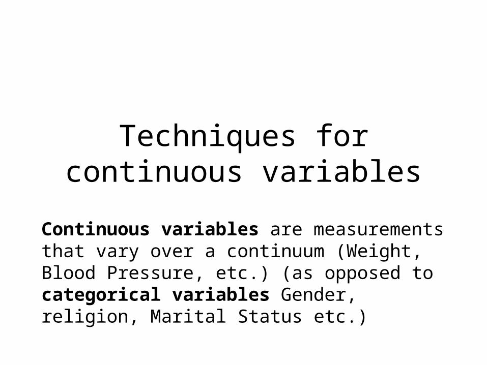
Techniques for continuous variables
Continuous variables are measurements that vary over a continuum (Weight, Blood Pressure, etc.) (as opposed to categorical variables Gender, religion, Marital Status etc.)

The Grouped frequency table:The Histogram

To Construct
• A Grouped frequency table
• A Histogram
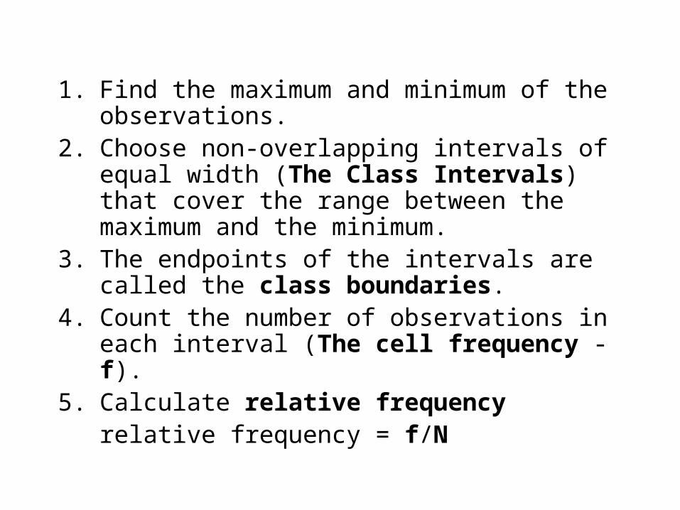
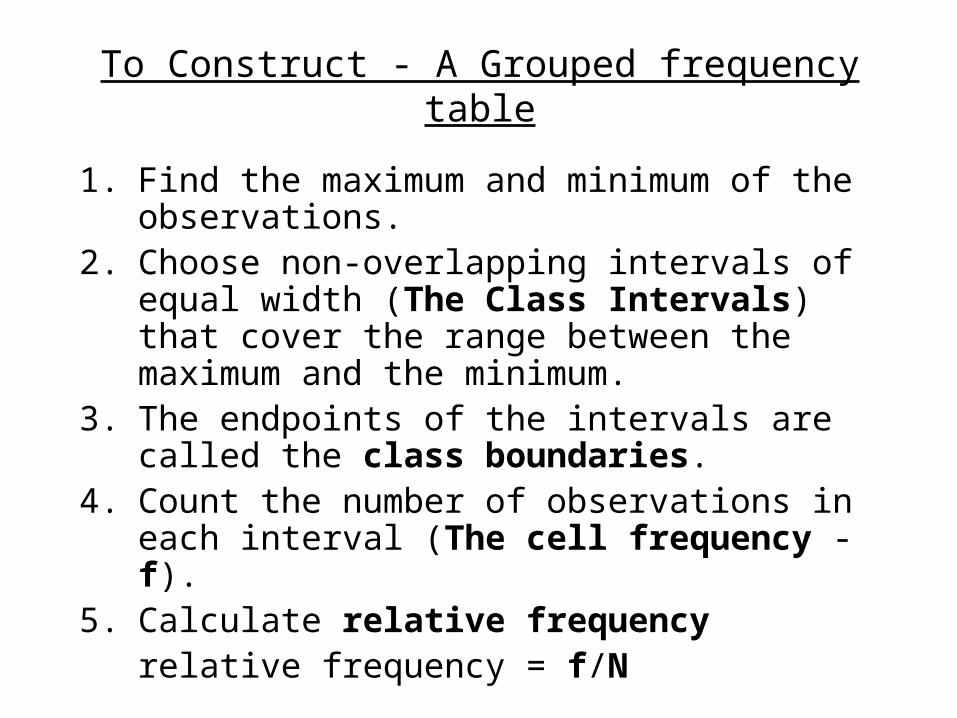
1. Find the maximum and minimum of the observations.
2. Choose non-overlapping intervals of equal width (The Class Intervals) that cover the range between the maximum and the minimum.
3. The endpoints of the intervals are called the class boundaries.
4. Count the number of observations in each interval (The cell frequency - f).
5. Calculate relative frequencyrelative frequency = f/N

Data Set #3
The following table gives data on Verbal IQ, Math IQ,Initial Reading Acheivement Score, and Final Reading Acheivement Score
for 23 students who have recently completed a reading improvement program
Initial FinalVerbal Math Reading Reading
Student IQ IQ Acheivement Acheivement
1 86 94 1.1 1.72 104 103 1.5 1.73 86 92 1.5 1.94 105 100 2.0 2.05 118 115 1.9 3.56 96 102 1.4 2.47 90 87 1.5 1.88 95 100 1.4 2.09 105 96 1.7 1.7
10 84 80 1.6 1.711 94 87 1.6 1.712 119 116 1.7 3.113 82 91 1.2 1.814 80 93 1.0 1.715 109 124 1.8 2.516 111 119 1.4 3.017 89 94 1.6 1.818 99 117 1.6 2.619 94 93 1.4 1.420 99 110 1.4 2.021 95 97 1.5 1.322 102 104 1.7 3.123 102 93 1.6 1.9
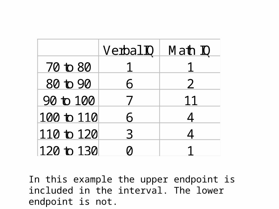
Verbal IQ Math IQ70 to 80 1 180 to 90 6 290 to 100 7 11
100 to 110 6 4110 to 120 3 4120 to 130 0 1
In this example the upper endpoint is included in the interval. The lower endpoint is not.
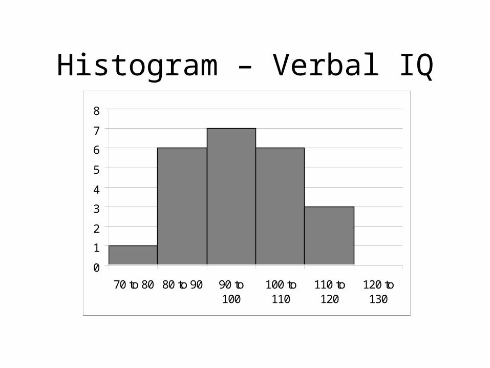
Histogram – Verbal IQ
0
1
2
3
4
5
6
7
8
70 to 80 80 to 90 90 to100
100 to110
110 to120
120 to130
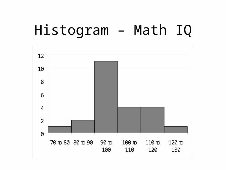
Histogram – Math IQ
0
2
4
6
8
10
12
70 to 80 80 to 90 90 to100
100 to110
110 to120
120 to130
Example
• In this example we are comparing (for two drugs A and B) the time to metabolize the drug.
• 120 cases were given drug A.
• 120 cases were given drug B.
• Data on time to metabolize each drug is given on the next two slides
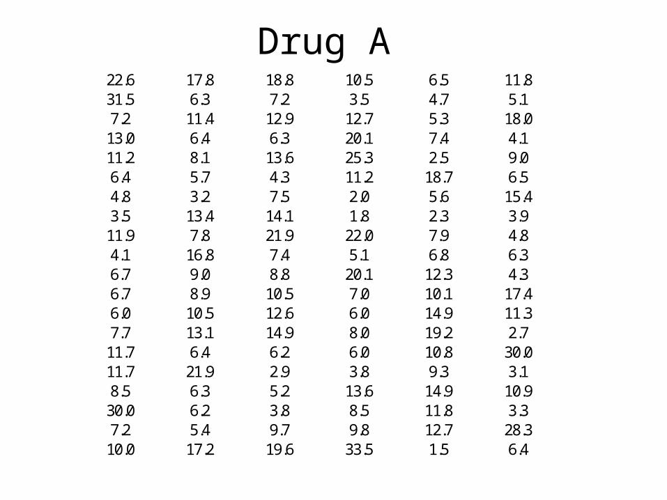
Drug A22.6 17.8 18.8 10.5 6.5 11.831.5 6.3 7.2 3.5 4.7 5.17.2 11.4 12.9 12.7 5.3 18.0
13.0 6.4 6.3 20.1 7.4 4.111.2 8.1 13.6 25.3 2.5 9.06.4 5.7 4.3 11.2 18.7 6.54.8 3.2 7.5 2.0 5.6 15.43.5 13.4 14.1 1.8 2.3 3.9
11.9 7.8 21.9 22.0 7.9 4.84.1 16.8 7.4 5.1 6.8 6.36.7 9.0 8.8 20.1 12.3 4.36.7 8.9 10.5 7.0 10.1 17.46.0 10.5 12.6 6.0 14.9 11.37.7 13.1 14.9 8.0 19.2 2.7
11.7 6.4 6.2 6.0 10.8 30.011.7 21.9 2.9 3.8 9.3 3.18.5 6.3 5.2 13.6 14.9 10.9
30.0 6.2 3.8 8.5 11.8 3.37.2 5.4 9.7 9.8 12.7 28.3
10.0 17.2 19.6 33.5 1.5 6.4
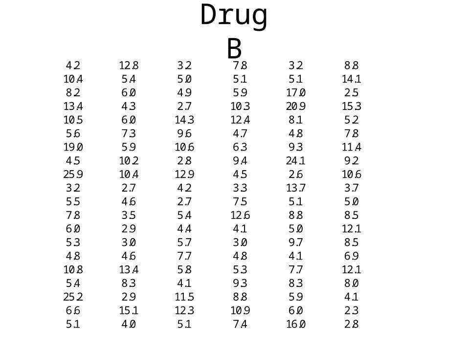
Drug B4.2 12.8 3.2 7.8 3.2 8.8
10.4 5.4 5.0 5.1 5.1 14.18.2 6.0 4.9 5.9 17.0 2.5
13.4 4.3 2.7 10.3 20.9 15.310.5 6.0 14.3 12.4 8.1 5.25.6 7.3 9.6 4.7 4.8 7.8
19.0 5.9 10.6 6.3 9.3 11.44.5 10.2 2.8 9.4 24.1 9.2
25.9 10.4 12.9 4.5 2.6 10.63.2 2.7 4.2 3.3 13.7 3.75.5 4.6 2.7 7.5 5.1 5.07.8 3.5 5.4 12.6 8.8 8.56.0 2.9 4.4 4.1 5.0 12.15.3 3.0 5.7 3.0 9.7 8.54.8 4.6 7.7 4.8 4.1 6.9
10.8 13.4 5.8 5.3 7.7 12.15.4 8.3 4.1 9.3 8.3 8.0
25.2 2.9 11.5 8.8 5.9 4.16.6 15.1 12.3 10.9 6.0 2.35.1 4.0 5.1 7.4 16.0 2.8
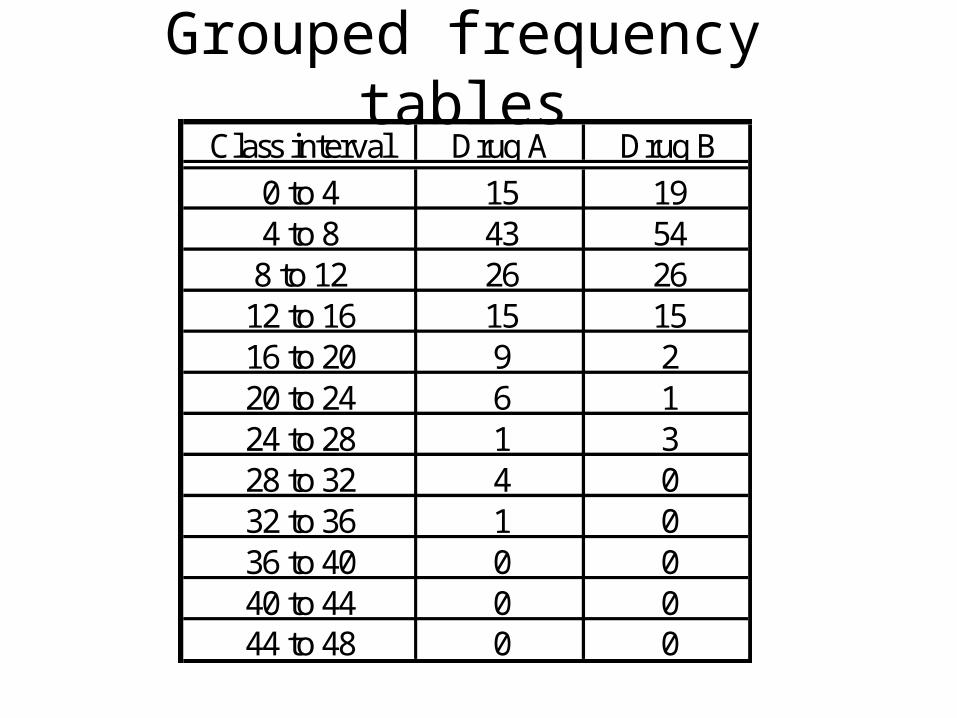
Grouped frequency tablesClass interval Drug A Drug B
0 to 4 15 194 to 8 43 54
8 to 12 26 2612 to 16 15 1516 to 20 9 220 to 24 6 124 to 28 1 328 to 32 4 032 to 36 1 036 to 40 0 040 to 44 0 044 to 48 0 0
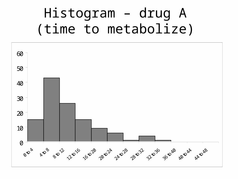
Histogram – drug A(time to metabolize)
0
10
20
30
40
50
60
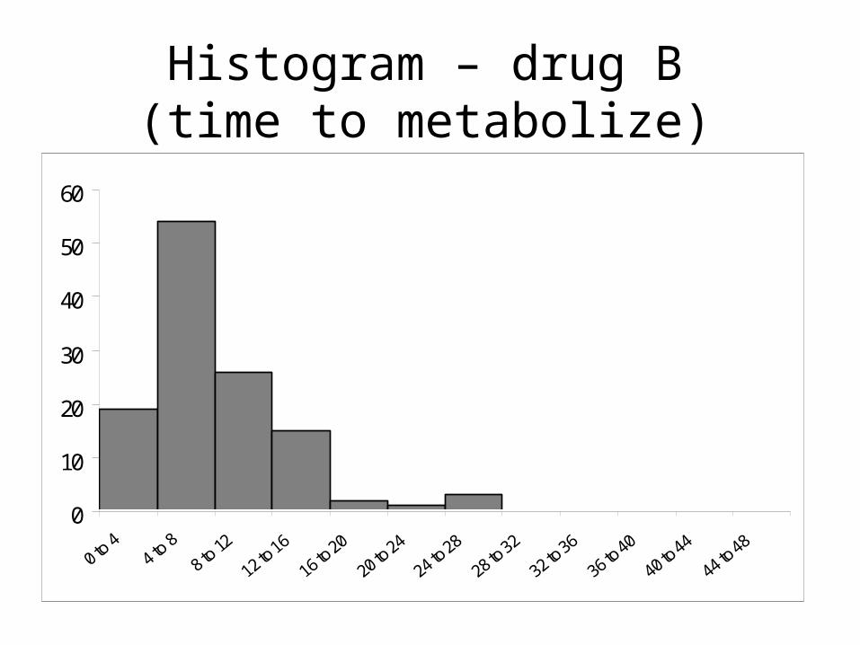
Histogram – drug B(time to metabolize)
0
10
20
30
40
50
60
The Grouped frequency table:The Histogram
To Construct
• A Grouped frequency table
• A Histogram
1. Find the maximum and minimum of the observations.
2. Choose non-overlapping intervals of equal width (The Class Intervals) that cover the range between the maximum and the minimum.
3. The endpoints of the intervals are called the class boundaries.
4. Count the number of observations in each interval (The cell frequency - f).
5. Calculate relative frequencyrelative frequency = f/N
To Construct - A Grouped frequency table
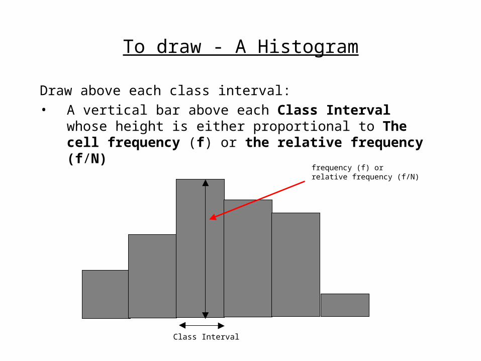
Draw above each class interval:
• A vertical bar above each Class Interval whose height is either proportional to The cell frequency (f) or the relative frequency (f/N)
To draw - A Histogram
Class Interval
frequency (f) or relative frequency (f/N)
Some comments about histograms
• The width of the class intervals should be chosen so that the number of intervals with a frequency less than 5 is small.
• This means that the width of the class intervals can decrease as the sample size increases
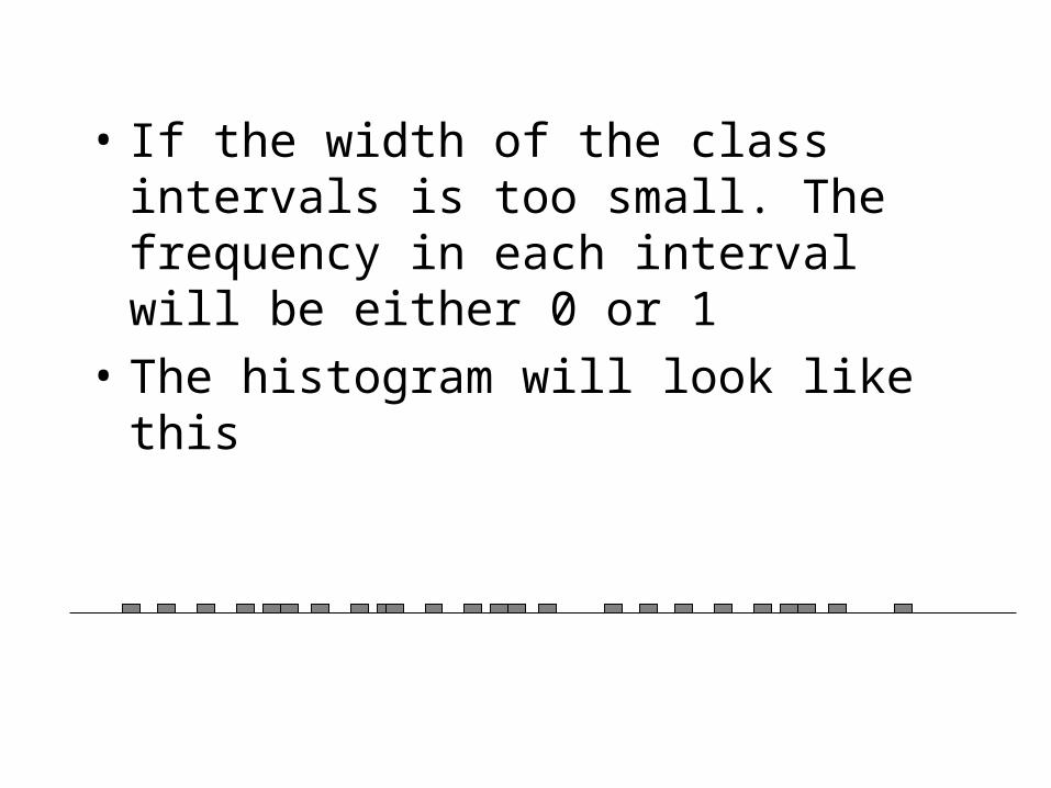
• If the width of the class intervals is too small. The frequency in each interval will be either 0 or 1
• The histogram will look like this
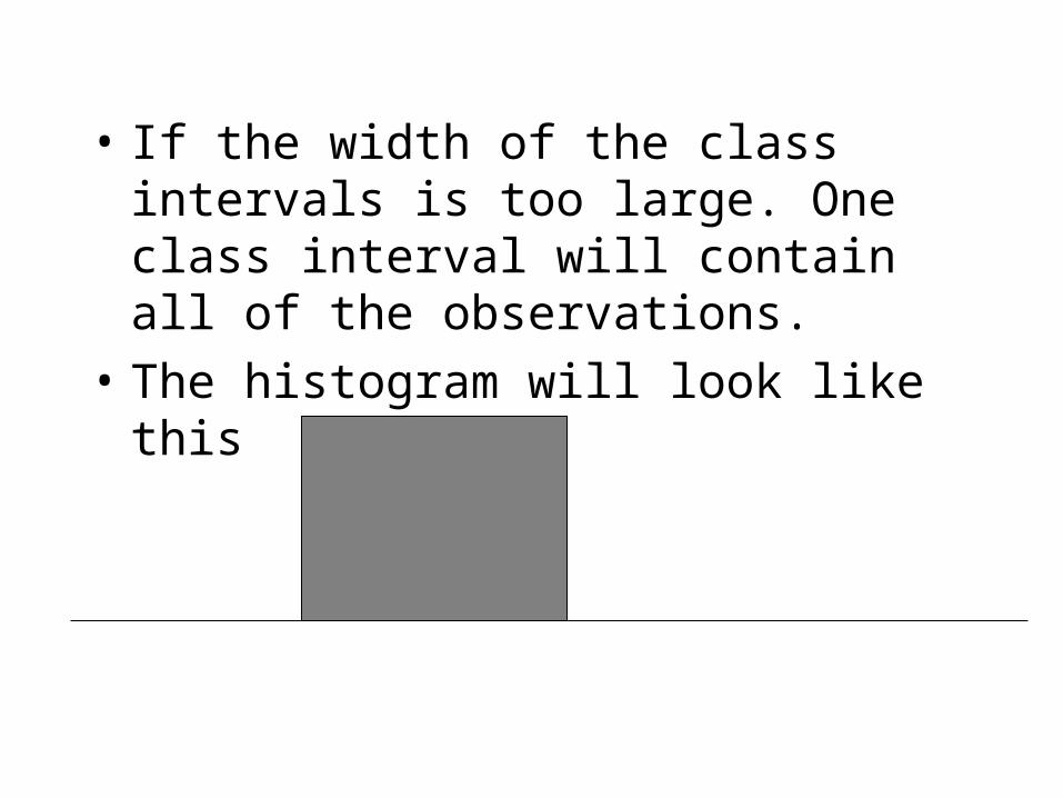
• If the width of the class intervals is too large. One class interval will contain all of the observations.
• The histogram will look like this
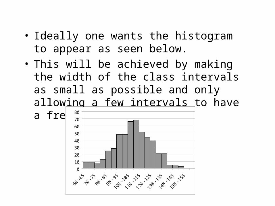
• Ideally one wants the histogram to appear as seen below.
• This will be achieved by making the width of the class intervals as small as possible and only allowing a few intervals to have a frequency less than 5.
0
10
20
30
40
50
60
70
80
60 -
65
70 -
75
80 -
85
90 -
95
100
- 105
110
- 115
120
- 125
130
- 135
140
- 145
150
- 155
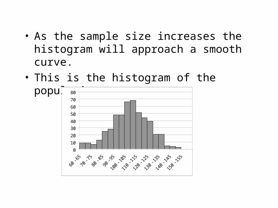
• As the sample size increases the histogram will approach a smooth curve.
• This is the histogram of the population
0
10
20
30
40
50
60
70
80
60 -
65
70 -
75
80 -
85
90 -
95
100
- 105
110
- 115
120
- 125
130
- 135
140
- 145
150
- 155
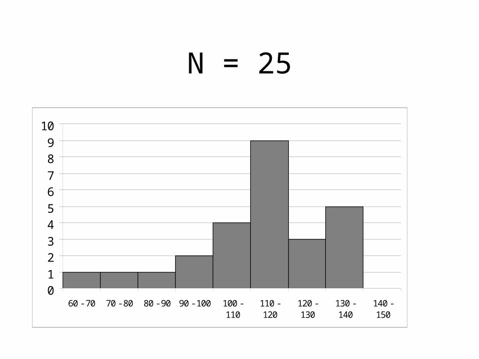
N = 25
01
23
45
67
89
10
60 - 70 70 - 80 80 - 90 90 - 100 100 -110
110 -120
120 -130
130 -140
140 -150
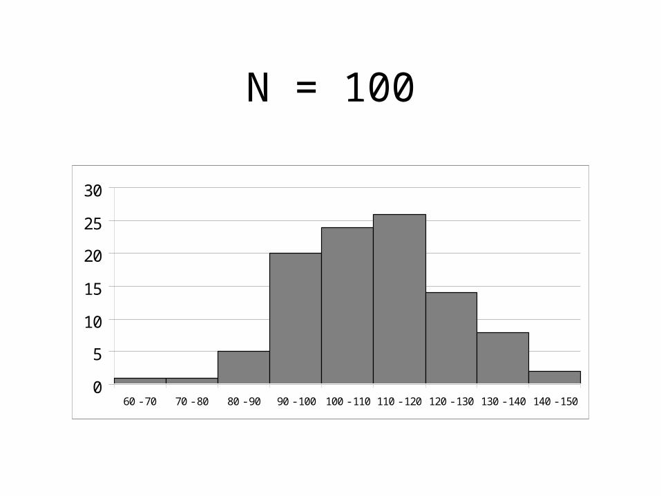
N = 100
0
5
10
15
20
25
30
60 - 70 70 - 80 80 - 90 90 - 100 100 - 110 110 - 120 120 - 130 130 - 140 140 - 150
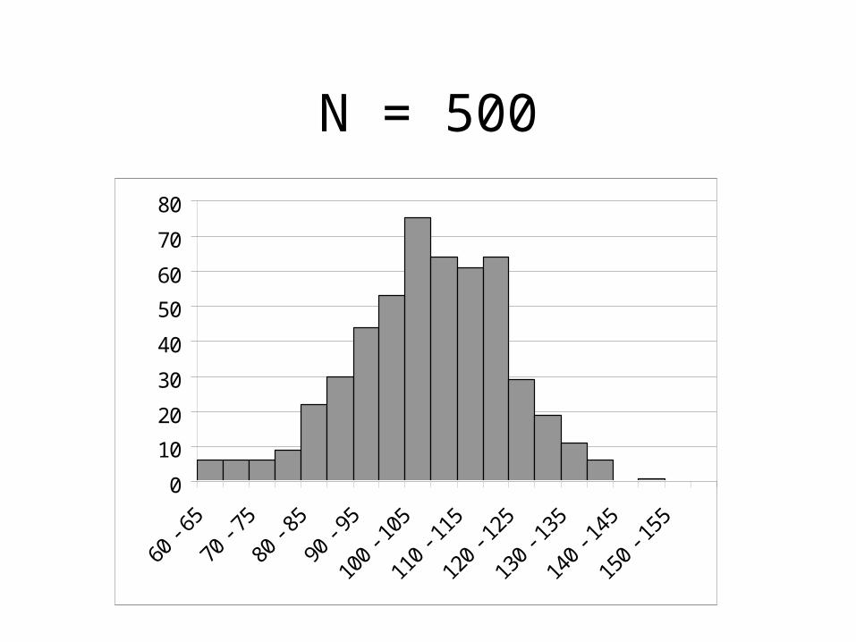
N = 500
0
10
20
30
40
50
60
70
80
60 -
65
70 -
75
80 -
85
90 -
95
100
- 105
110
- 115
120
- 125
130
- 135
140
- 145
150
- 155
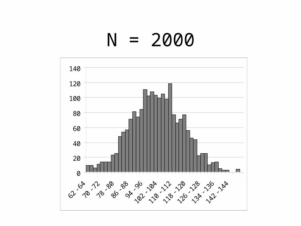
N = 2000
0
20
40
60
80
100
120
140
62 -
64
70 -
72
78 -
80
86 -
88
94 -
96
102
- 104
110
- 112
118
- 120
126
- 128
134
- 136
142
- 144
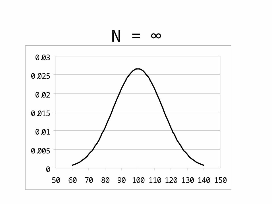
N = ∞
0
0.005
0.01
0.015
0.02
0.025
0.03
50 60 70 80 90 100 110 120 130 140 150
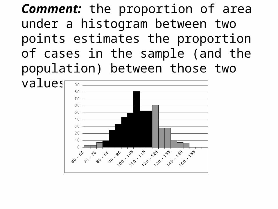
Comment: the proportion of area under a histogram between two points estimates the proportion of cases in the sample (and the population) between those two values.
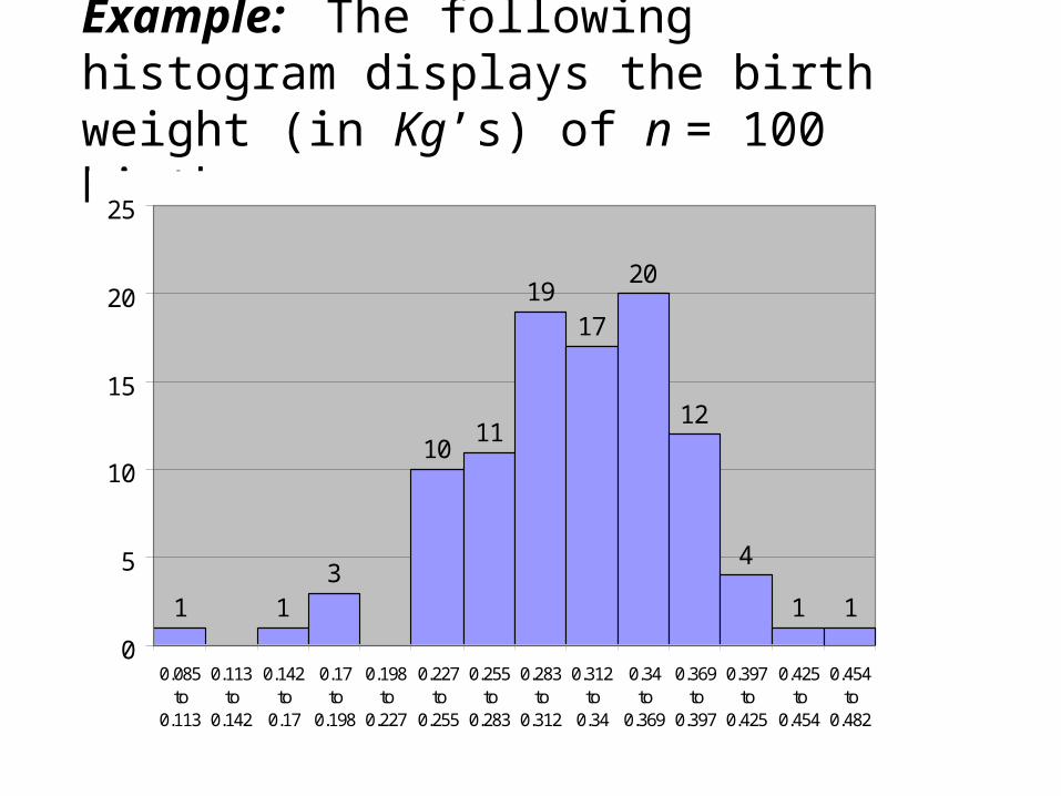
Example: The following histogram displays the birth weight (in Kg’s) of n = 100 births
1 13
1011
1917
20
12
4
1 1
0
5
10
15
20
25
0.085to
0.113
0.113to
0.142
0.142to
0.17
0.17to
0.198
0.198to
0.227
0.227to
0.255
0.255to
0.283
0.283to
0.312
0.312to
0.34
0.34to
0.369
0.369to
0.397
0.397to
0.425
0.425to
0.454
0.454to
0.482
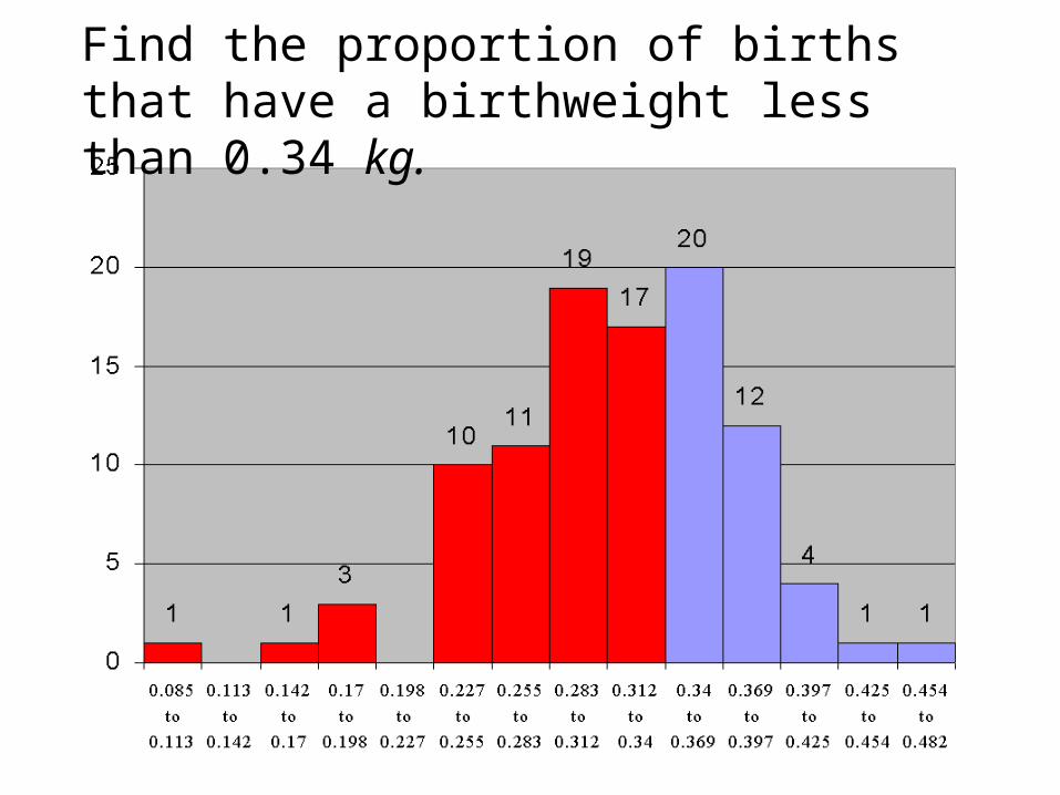
Find the proportion of births that have a birthweight less than 0.34 kg.
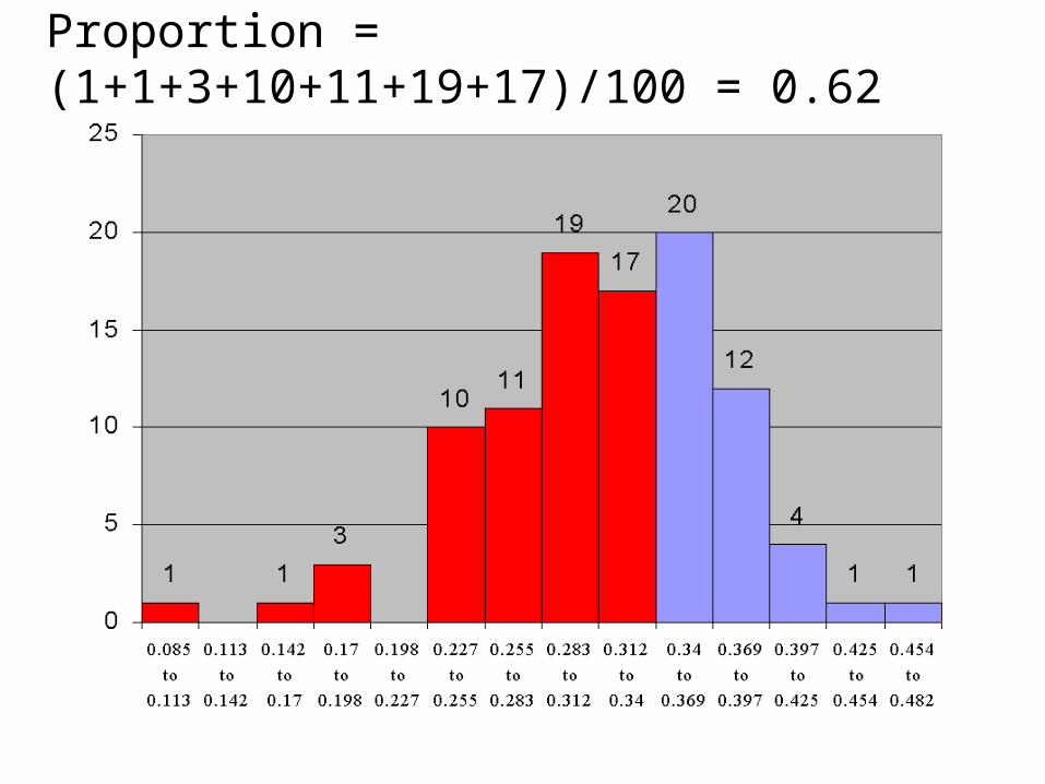
Proportion = (1+1+3+10+11+19+17)/100 = 0.62
The Characteristics of a Histogram
• Central Location (average)
• Spread (Variability, Dispersion)
• Shape
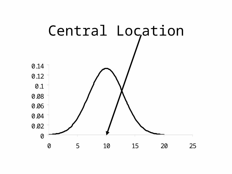
Central Location
0
0.02
0.04
0.06
0.08
0.1
0.12
0.14
0 5 10 15 20 25
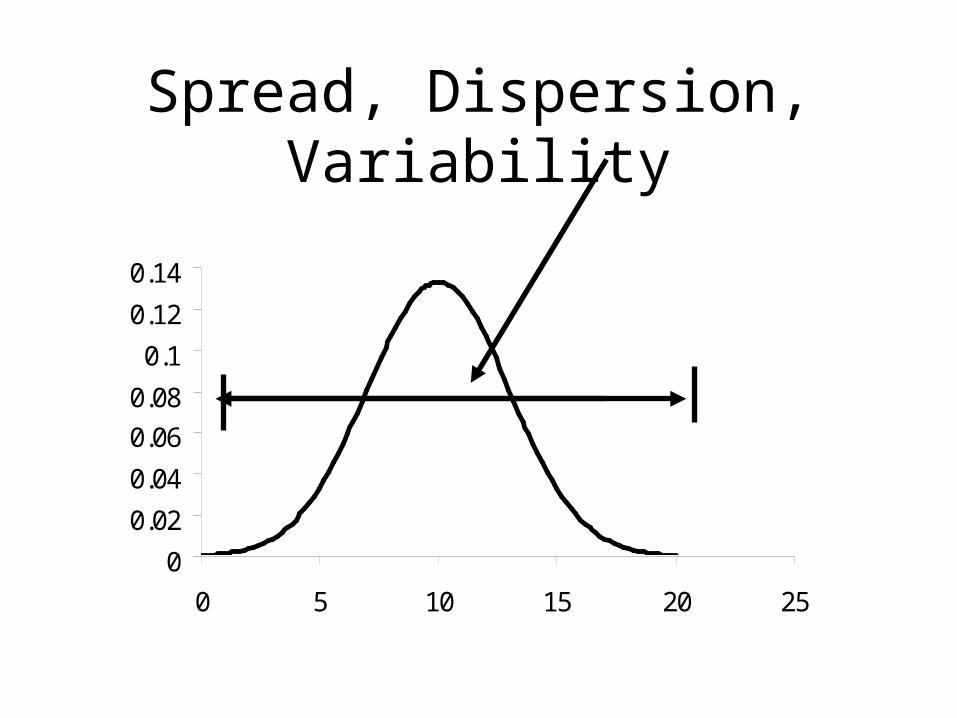
Spread, Dispersion, Variability
0
0.02
0.04
0.06
0.08
0.1
0.12
0.14
0 5 10 15 20 25
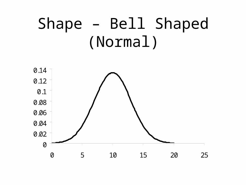
Shape – Bell Shaped (Normal)
0
0.02
0.04
0.06
0.08
0.1
0.12
0.14
0 5 10 15 20 25
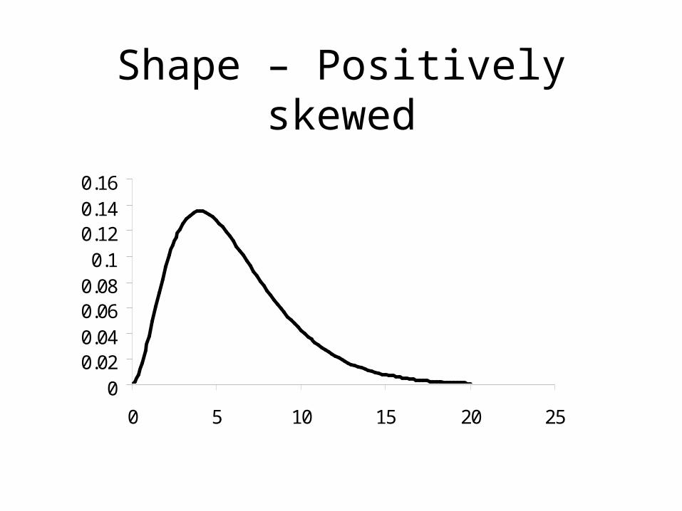
Shape – Positively skewed
00.020.040.060.080.1
0.120.140.16
0 5 10 15 20 25
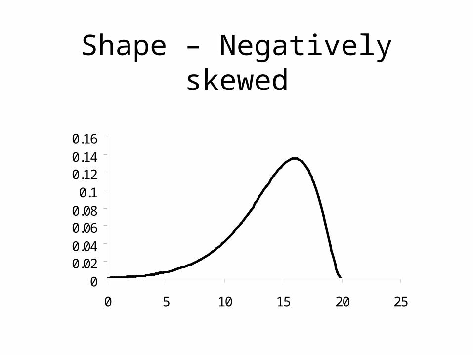
Shape – Negatively skewed
00.020.040.060.080.1
0.120.140.16
0 5 10 15 20 25
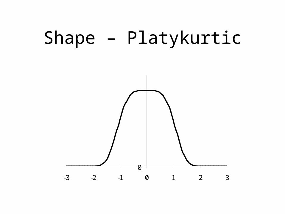
Shape – Platykurtic
0
-3 -2 -1 0 1 2 3
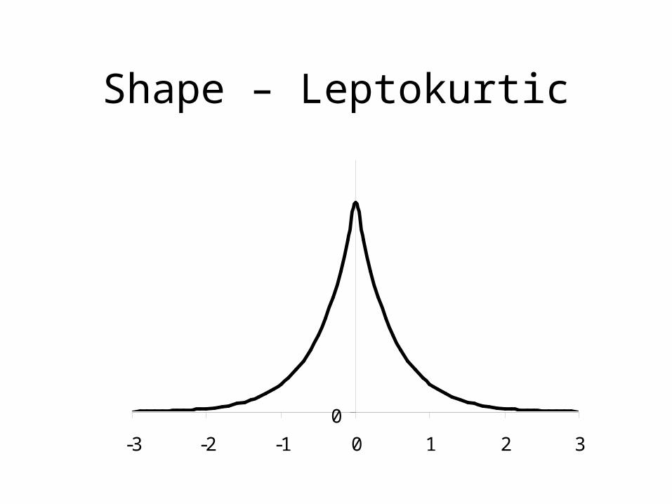
Shape – Leptokurtic
0
-3 -2 -1 0 1 2 3
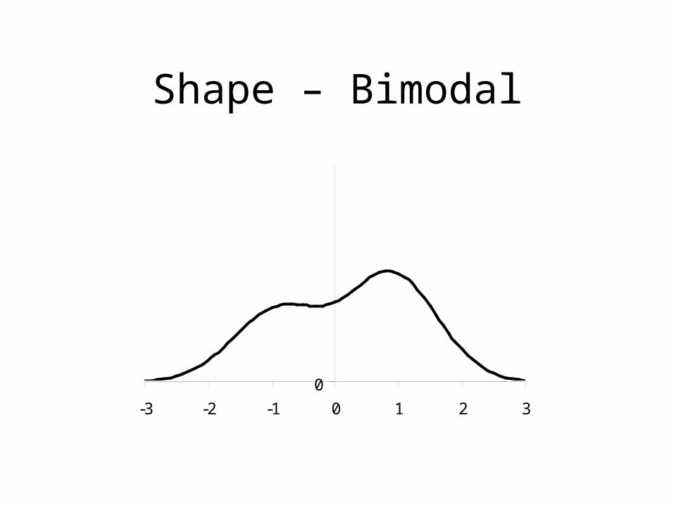
Shape – Bimodal
0
-3 -2 -1 0 1 2 3

The Stem-Leaf Plot
An alternative to the histogram
Each number in a data set can be broken into two parts
– A stem
– A Leaf
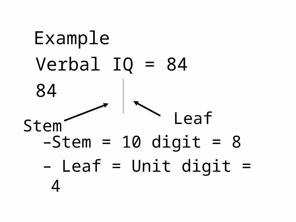
Example
Verbal IQ = 84
84
–Stem = 10 digit = 8
– Leaf = Unit digit = 4
LeafStem
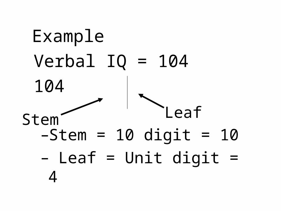
Example
Verbal IQ = 104
104
–Stem = 10 digit = 10
– Leaf = Unit digit = 4
LeafStem
To Construct a Stem- Leaf diagram
• Make a vertical list of “all” stems
• Then behind each stem make a horizontal list of each leaf
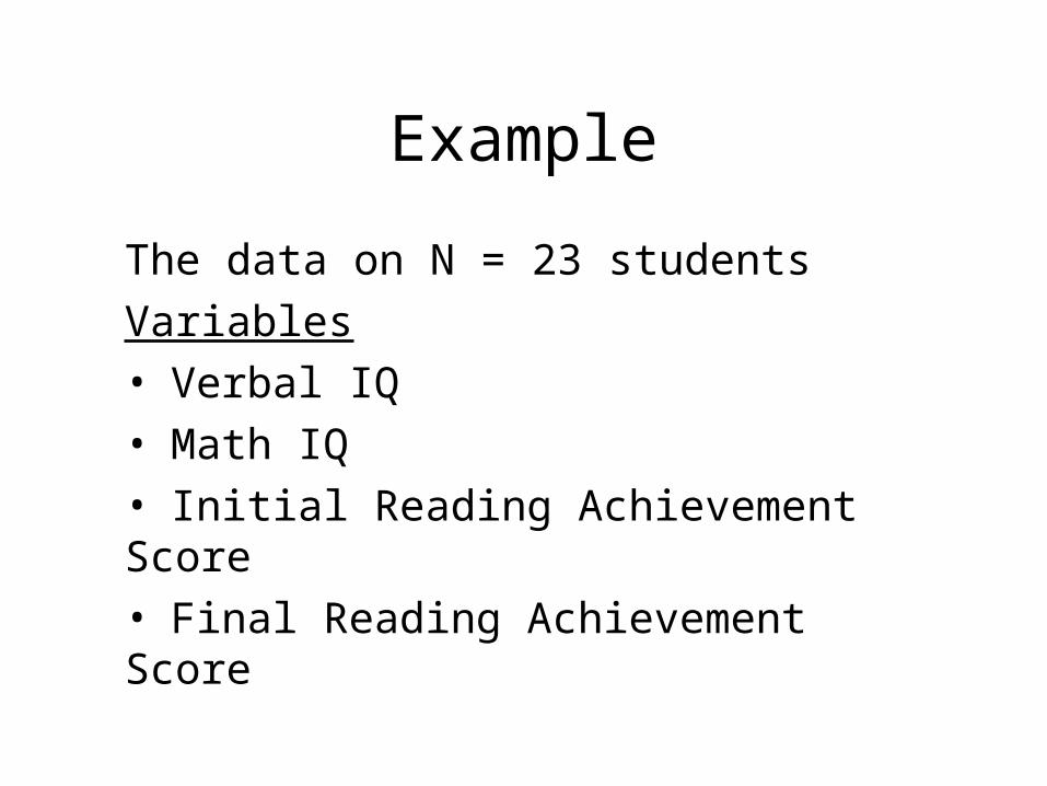
Example
The data on N = 23 students
Variables
• Verbal IQ
• Math IQ
• Initial Reading Achievement Score
• Final Reading Achievement Score
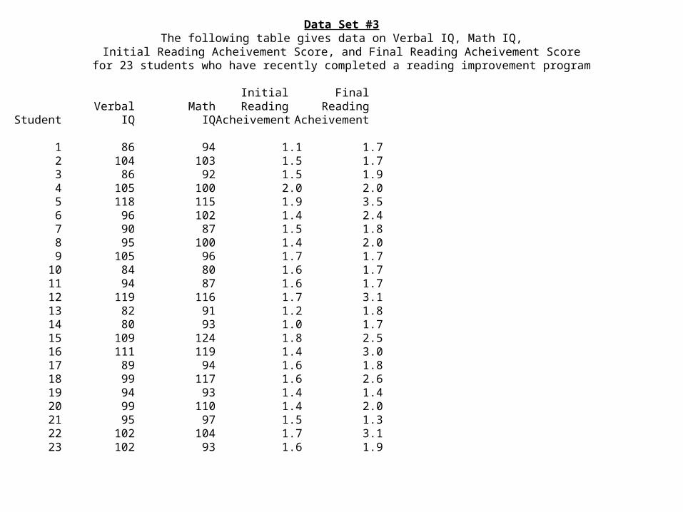
Data Set #3
The following table gives data on Verbal IQ, Math IQ,Initial Reading Acheivement Score, and Final Reading Acheivement Score
for 23 students who have recently completed a reading improvement program
Initial FinalVerbal Math Reading Reading
Student IQ IQ Acheivement Acheivement
1 86 94 1.1 1.72 104 103 1.5 1.73 86 92 1.5 1.94 105 100 2.0 2.05 118 115 1.9 3.56 96 102 1.4 2.47 90 87 1.5 1.88 95 100 1.4 2.09 105 96 1.7 1.7
10 84 80 1.6 1.711 94 87 1.6 1.712 119 116 1.7 3.113 82 91 1.2 1.814 80 93 1.0 1.715 109 124 1.8 2.516 111 119 1.4 3.017 89 94 1.6 1.818 99 117 1.6 2.619 94 93 1.4 1.420 99 110 1.4 2.021 95 97 1.5 1.322 102 104 1.7 3.123 102 93 1.6 1.9
We now construct:
a stem-Leaf diagram
of Verbal IQ
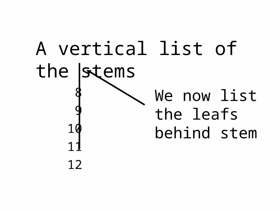
A vertical list of the stems8
9
10
11
12
We now list the leafs behind stem
8
9
10
11
12
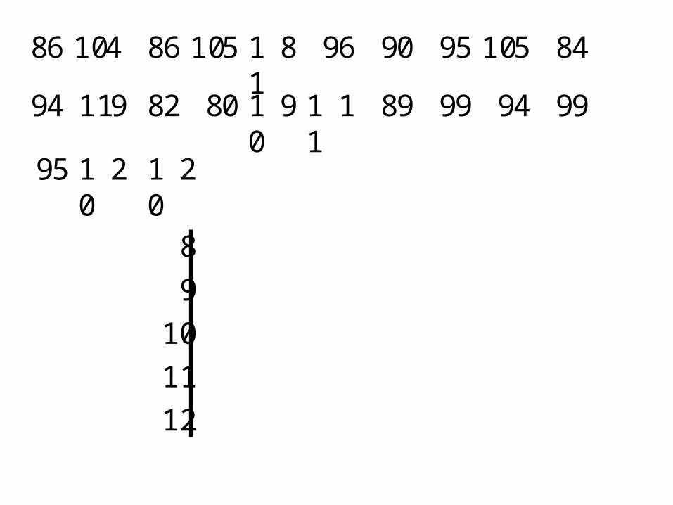
86 104 86 105 118 96 90 95 105 84
94 119 82 80 109 111 89 99 94 99
95 102 102
8
9
10
11
12
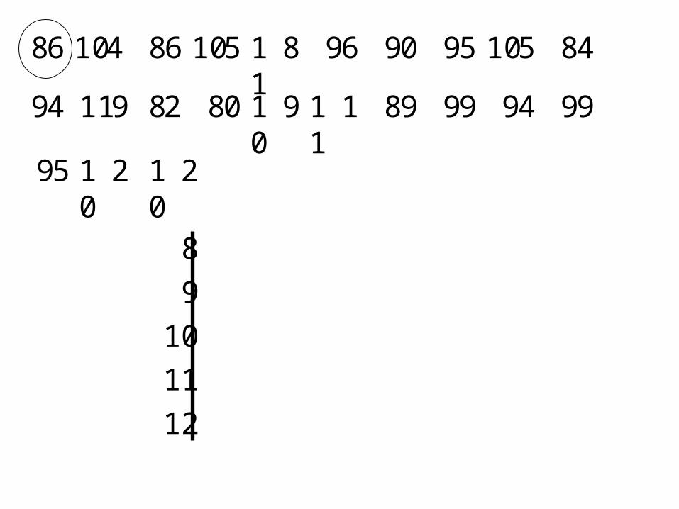
86 104 86 105 118 96 90 95 105 84
94 119 82 80 109 111 89 99 94 99
95 102 102
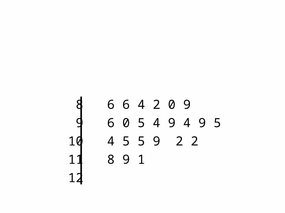
8 6 6 4 2 0 9
9 6 0 5 4 9 4 9 5
10 4 5 5 9 2 2
11 8 9 1
12
8 0 2 4 6 6 9
9 0 4 4 5 5 6 9 9
10 2 2 4 5 5 9
11 1 8 9
12
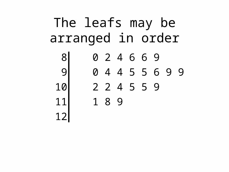
The leafs may be arranged in order
8 0 2 4 6 6 9
9 0 4 4 5 5 6 9 9
10 2 2 4 5 5 9
11 1 8 9
12
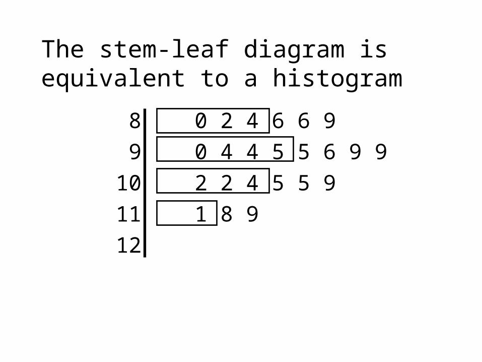
The stem-leaf diagram is equivalent to a histogram

8 0 2 4 6 6 9
9 0 4 4 5 5 6 9 9
10 2 2 4 5 5 9
11 1 8 9
12
The stem-leaf diagram is equivalent to a histogram
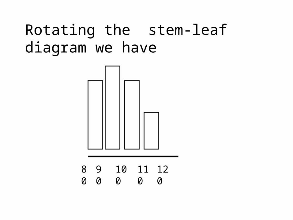
Rotating the stem-leaf diagram we have
80 90 100 110 120
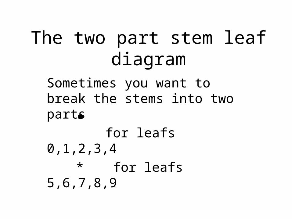
The two part stem leaf diagram
Sometimes you want to break the stems into two parts
for leafs 0,1,2,3,4
* for leafs 5,6,7,8,9
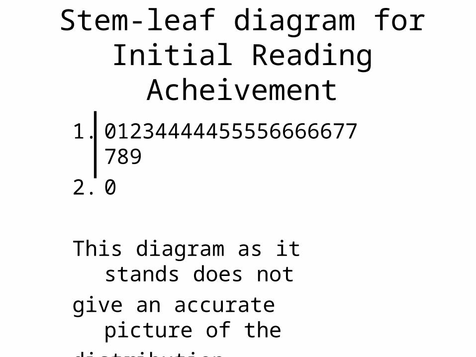
Stem-leaf diagram for Initial Reading Acheivement
1. 01234444455556666677789
2. 0
This diagram as it stands does not
give an accurate picture of the
distribution
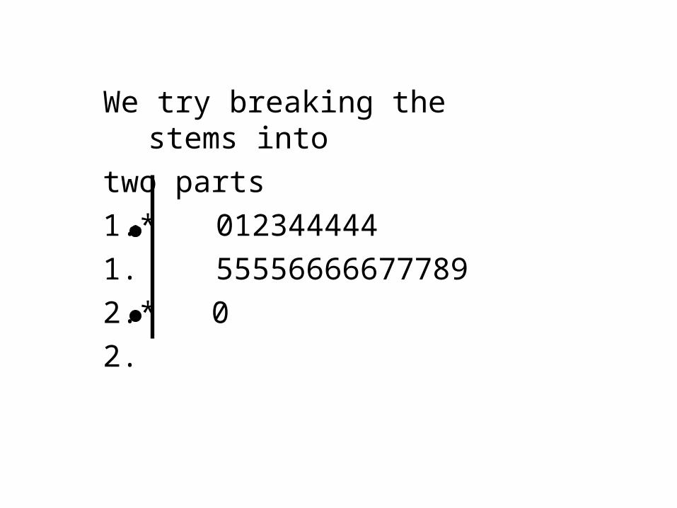
We try breaking the stems into
two parts
1.* 012344444
1. 55556666677789
2.* 0
2.
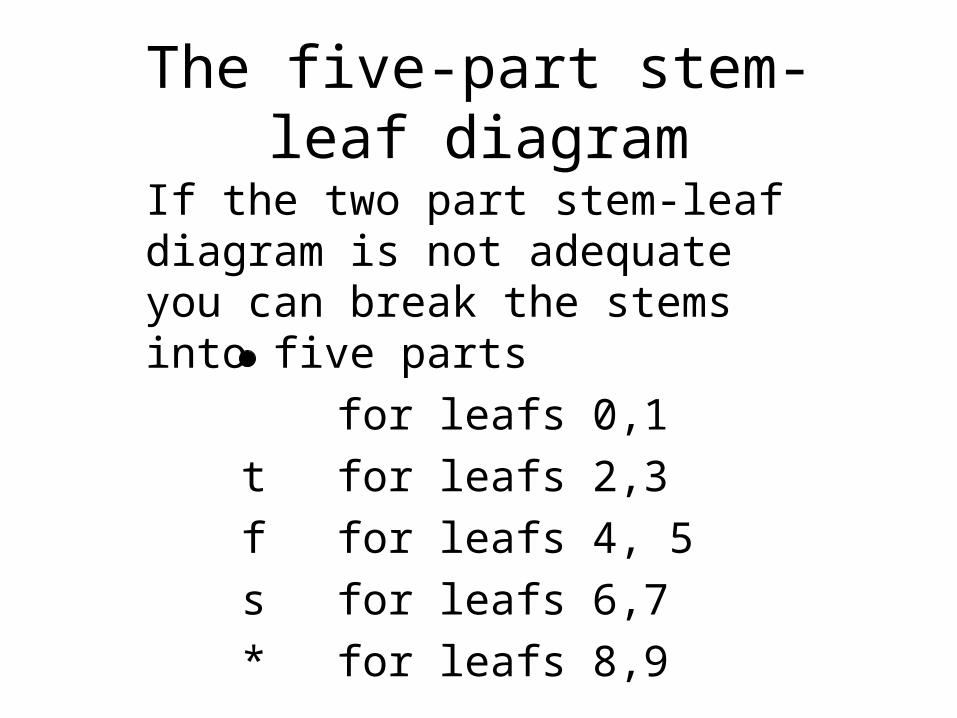
The five-part stem-leaf diagram
If the two part stem-leaf diagram is not adequate you can break the stems into five parts
for leafs 0,1
t for leafs 2,3
f for leafs 4, 5
s for leafs 6,7
* for leafs 8,9
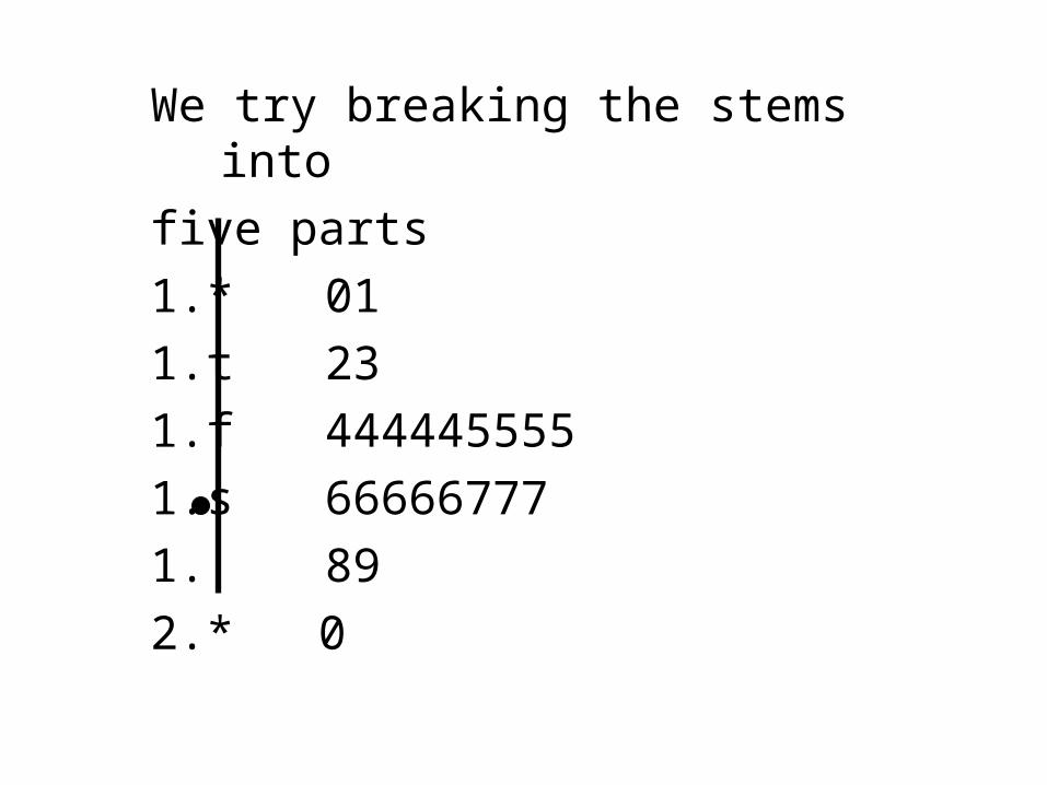
We try breaking the stems into
five parts
1.* 01
1.t 23
1.f 444445555
1.s 66666777
1. 89
2.* 0
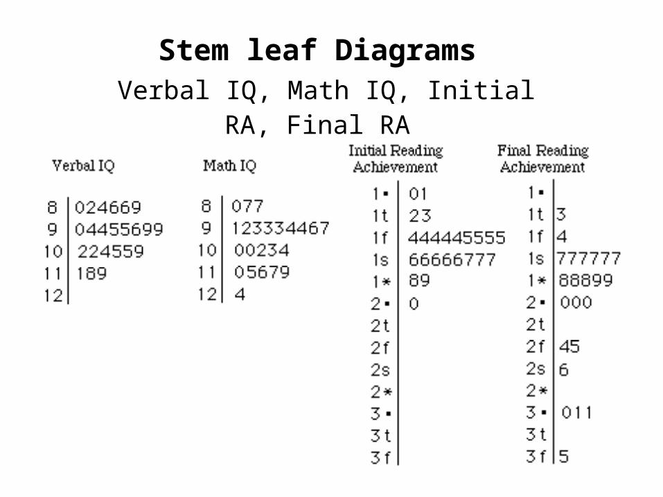
Stem leaf Diagrams
Verbal IQ, Math IQ, Initial RA, Final RA
Some Conclusions
• Math IQ, Verbal IQ seem to have approximately the same distribution
• “bell shaped” centered about 100
• Final RA seems to be larger than initial RA and more spread out
• Improvement in RA
• Amount of improvement quite variable
Next Topic
• Numerical Measures - Location


![TABLOID - 11 x 17...9 9 8 8 7 7 6 6 5 5 4 4 3 3 2 2 1 1 A A C C E E G G H H J J K K L L M M N N O O 20'-0" [(6096 mm)] 20'-0" [(6096 mm)] 20'-0" [(6096 mm)] 20'-0" [(6096 mm)] 20'-0"](https://img.pdfslide.net/doc/110x75/614902ff9241b00fbd674892/tabloid-11-x-17-9-9-8-8-7-7-6-6-5-5-4-4-3-3-2-2-1-1-a-a-c-c-e-e-g-g-h-h-j.jpg)