Embed Size (px)
Citation preview
15
C H A P T E R 1
Orientation to Transport Networks and Technology
Many readers will have an initial picture of how thetelecommunication network operates that is based on telephony circuit switching. This involvesthe switching of individual voice circuits through a network of trunk groups. Historically thetrunk groups were cables comprising many twisted wire pairs and switching involved metallicconnections between wire pairs in these trunk cables. Later, in the first step toward virtualiza-tion, point-to-point carrier transmission systems created more than one logical channel pertwisted pair, and switching evolved to making connections between these logical channels. Butin this context the transmission systems only provided “pair gain” between the switching nodes.In a second important step, cross-connect panels or cross-connect machines began to provideinterconnection directly between carrier systems so that the apparent network seen by the cir-cuit-switching machines could be rearranged at will. The same evolution has been repeated withwavelength division multiplexed (WDM) transmission, from point-to-point “pair gain” withcoarse WDM, then to optical transport networking using dense WDM and optical cross-con-nects. In both cases the flexible interconnection of multiplexed carrier signals allows creation ofvirtual logical connectivity and capacity patterns for client service networks. This is the funda-mental idea of transport networking regardless of the technology involved.
Through transport networking, an essentially fixed set of multi-channel point-to-pointtransmission systems are managed to create virtual network environments for all other services.Today, for example, the logical model of voice circuit switching still holds but the entire tele-phone trunk network is virtual. There are no actual twisted pair cables between voice switches.Nor are there cables or fibers dedicated between IP routers or cables that “belong” to a bankingnetwork or private company network. All these networks operate logically as if they did havetheir own dedicated transmission systems, but they are each just one of several virtual “servicelayer” networks supported by one underlying actual network; the transport network.
Grover.book Page 15 Sunday, July 20, 2003 3:46 PM
16 Chapter 1 • Orientation to Transport Networks and Technology
Another widespread concept is packet switching. A compelling but oversimplified notionis that each packet takes an independent route through the network directly over the physical-layer cables. In reality, aggregations of data packets with common destinations or intermediatehubs en route are formed near the edges of the network and then follow preestablished logicalconduits without further packet-by-packet inspection until they are near or at their destination.These logical conduits appear to the packet-switching nodes to be dedicated point-to-point trans-mission systems, but in fact they are cross-connected paths through the transport network, pro-viding the logical network for the packet-switching service.
Both of these familiar types of network (e.g., circuit-switched telephony and packet dataswitching) have in recent times become essentially virtual. They are only examples of special-ized service layer networks operating over a common transport network. It is natural for us alsoto perceive and interact with other services such as the Internet, the banking network (ATMmachines), credit verification, travel booking networks, and so on, as if they were separate phys-ical networks. But they are all just logical abstractions created within one physical network bylogical configuration of the carrier signals borne on fiber optic strands. Individual telephonecalls, packet streams, leased lines, ATM trunks, Internet connections, etc., do not make theirown way natively over the fiber systems. Rather, aggregations of all traffic types from site tosite are formed by multiplexing these payloads up to a set of standard-rate digital carrier signalsof rates such as DS3, STS1, STS3c and so on, to be discussed. Traffic of all sources, sometimeseven from competing service providers, is combined (by statistical multiplexing or time divisionmultiplexing) into composite digital signal streams for assignment to a given wavelength path orfiber route through the physical network.
The transport network operates below these user-perceived service networks, and abovethe fixed physical network, to “serve up” logical connectivity requirements to such client net-works from the underlying physical base of transmission resources. This client-server relation-ship can sometimes be observed across several layers. For instance, an optical transport networkmay implement lightpaths to create the logical topology for a SONET OC-192 network. ThatSONET network may itself provide routing and cross-connection for a mixture of logical pathsand a variety of connection rates and types such as Gigabit Ethernet, ATM, IP, and DS3, or DS1leased lines. An ATM client network of the SONET layer may itself then provide transport forvarious IP flows between Internet routers, and so on. Thus transport can also be thought of as aninter layer relationship, not always a single identifiable layer in its own right. An important tech-nological drive is, however, to reduce this historical accumulation of layers to a single layer-pair: that of “IP over optics.” This is an important development to which we will return. “IP overoptics” both simplifies and enhances the application of the network design methods that follow.
The mandate of this chapter is to establish familiarity with the basic concepts of transportnetworking, the technologies used, and some of the important issues that distinguish transportnetworking from other far more dominant networking concepts. This establishes context for thedesign problems that follow and equips a student to understand and explain to others—such as ata thesis defense—how it is, for example, that we don’t see individual packet routing consider-
Grover.book Page 16 Sunday, July 20, 2003 3:46 PM
17
ations in a transport layer study, or how it can be that some nodes of the actual network do notappear in the transport network graph. (“Does it mean you have decided not to provide service tothose cities?”) These questions, both of which were earnestly posed by committee members tothe authors students during their dissertations, are typical of the misunderstandings about, orsimple unawareness about, the concept of transport networking. Thus, there is a real need forstudents and practitioners to understand transport as a networking paradigm of its own, differentfrom telephony switching and packet switching as well as leased-line private network design,and to be able to give clarifying answers to questions such as above. However, space permitsonly a basic introduction to transport networking; the minimum needed to support later develop-ments in the book. To delve deeper, the book by K.Sato [Sato96] is recommended as a supple-ment. It gives a more extensive treatment of key ideas and technologies for transport networkingwithout considering network design or survivability.
1.0.1 Aggregation of Service Layer Traffic into Transport Demands
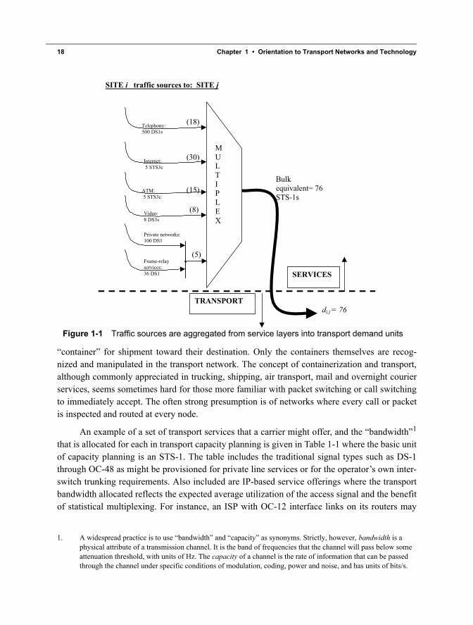
Ultimately, whether through IP over optics or through a stack of DS-3, ATM and SONETlayers, the net effect is that a set of user services is mapped onto a set of physical high-capacitytransmission, multiplexing and signal switching facilities that provide transmission paths to sup-port the logical connectivity and capacity requirements of all service layer flows. The aggrega-tion of flows between each pair of nodes on the transport network defines what is called thedemand on the transport network (or the respective transport layer). The term demand has a spe-cialized meaning, distinct from the more general term traffic [Wu92]. A demand unit is a quan-tum of transmission and routing capacity used to serve any aggregations of traffic flow from theservice layers. Whereas traffic may refer to measures of voice, data, or video flow intensities(Erlangs, packets per second, Mb/s, frames/sec, etc.), demands on a transport network are speci-fied in terms of the number of managed units of transmission capacity that the aggregation oftraffic requires. Demand may thus take on standard transmission units such as lightpaths, OC-192s, OC-48s, DS3s or DS1s. An optical backbone network may typically be managed at theOC-48 (~2.5 Gb/s of aggregated data) and the whole lightpath (i.e., contiguous optical carriersignal frequency assignments) level. Each lightpath could be formatted to carry an OC-192 thatmay be structured as 4 OC-48s or to carry a 10GigE aggregation of Ethernet packet frames, ormany other application-specific payload formats for which mappings are defined. These are justexamples of the general concept of aggregations of payload being matched onto standard unitsof demand for routing and capacity management in the transport layer.
Figure 1-1 illustrates the basic concept of multiple traffic sources being aggregated basedon their common destination (or a route to a common intermediate destination) thereby generat-ing a demand requirement on the transport network. In the example, the bulk equivalent of 76STS-1s would in practice be likely to generate two OC-48 demands.
It is important to note that, as the word “transport” suggests in general language, the indi-vidual packets, cells, phone calls, leased lines, and so on are no longer recognized or individu-ally processed at the nodes en route. In effect they have been grouped together in a standard
Grover.book Page 17 Sunday, July 20, 2003 3:46 PM
18 Chapter 1 • Orientation to Transport Networks and Technology
“container” for shipment toward their destination. Only the containers themselves are recog-nized and manipulated in the transport network. The concept of containerization and transport,although commonly appreciated in trucking, shipping, air transport, mail and overnight courierservices, seems sometimes hard for those more familiar with packet switching or call switchingto immediately accept. The often strong presumption is of networks where every call or packetis inspected and routed at every node.
An example of a set of transport services that a carrier might offer, and the “bandwidth”1
that is allocated for each in transport capacity planning is given in Table 1-1 where the basic unitof capacity planning is an STS-1. The table includes the traditional signal types such as DS-1through OC-48 as might be provisioned for private line services or for the operator’s own inter-switch trunking requirements. Also included are IP-based service offerings where the transportbandwidth allocated reflects the expected average utilization of the access signal and the benefitof statistical multiplexing. For instance, an ISP with OC-12 interface links on its routers may
1. A widespread practice is to use “bandwidth” and “capacity” as synonyms. Strictly, however, bandwidth is a physical attribute of a transmission channel. It is the band of frequencies that the channel will pass below some attenuation threshold, with units of Hz. The capacity of a channel is the rate of information that can be passed through the channel under specific conditions of modulation, coding, power and noise, and has units of bits/s.
di,j = 76
M U L T I P L E X
Telephony: 500 DS1s
ATM: 5 STS3c
Video: 8 DS3s
Private networks: 100 DS1
Frame-relay services: 36 DS1
SITE i traffic sources to: SITE j
SERVICES
TRANSPORT
Bulk equivalent= 76 STS-1s
(18)
(30)
(15)
(8)
(5)
Internet: 5 STS3c
Figure 1-1 Traffic sources are aggregated from service layers into transport demand units
Grover.book Page 18 Sunday, July 20, 2003 3:46 PM

19
request a “private line” OC-12 as the bit-pipe to another router. Such a “PL” OC-12 will be atrue OC-12 circuit for which 12 STS-1s are allocated. Alternately, it may be an “IP” OC-12 ser-vice in which case a bandwidth of only about 13% of an actual OC-12 is allocated. The latter,obviously lower-cost, service essentially just provides an OC-12 access interface, from whichthe IP payloads will be extracted and statistically multiplexed with other flows in the carrier’snetwork. Table 1-1 and Figure 1-1 are just examples. The general point is that in operation anddesign of a transport network we deal with demand requirements posed in some basic unit oftransmission capacity. These requirements are generated by the aggregation of all types of ser-vice traffic. But in the transport network we generally never see or have to consider individualpackets or phone calls, etc., directly again.
In [DoHa98] the processes of bandwidth allocation based on service types, and overall ofaggregation of point-to-point bandwidth requirements to define a demand matrix for transportnetwork design, are described further. That paper also describes an overall framework of a net-work planning tool—the Integrated Network Design Tool (INDT)—that is relevant as an exam-ple of the kind of network planning software tool where many of the design methods in the Part2 chapters of this book would be employed in future.
1.0.2 Concept of Logical versus Physical Networks: Virtual TopologyEach fiber optic transmission system is itself an essentially fixed point-to-point structure
that bears whatever set of tributary carrier signals or wavelengths are presented to its inputs, upto its maximum capacity. Changes in the physical layer can be made, but on a much longer timescale than required for purely logical reconfigurations in the transport network. The set of tribu-
Table 1-1 Transport capacity allocated for various service types (STS-1 equivalents)a
a. PL = private line service in stipulated format, IP = IP packet service with specified interface rate and format, WL = wavelength service bearing OC-48 or OC-192 container format.
Service Capacity Service Capacity
DS-1 PL 0.036 IP-OC3 0.382
DS-3 PL 1.0 IP-OC12 1.528
OC-3 PL 3.0 IP-OC48 6.112
OC-12 PL 12.0 IP-100T (Ethernet) 0.283
OC-48 PL 48.0 IP-GIGE (Ethernet) 2.830
IP-DS1 0.005 WL-2.5G 48.000
IP-DS3 0.127 WL-10G 96.000
Grover.book Page 19 Sunday, July 20, 2003 3:46 PM
20 Chapter 1 • Orientation to Transport Networks and Technology
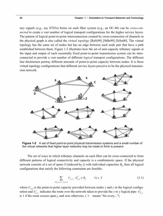
tary signals (e.g., say STS3s) borne on each fiber system (e.g., an OC-48) can be cross-con-nected to create a vast number of logical transport configurations for the higher service layers.The pattern of logical point-to-point interconnection created by cross-connection of channels inthe physical graph is also called the virtual topology [RaSi98] [StBa99] [SiSu00]. The virtualtopology has the same set of nodes but has an edge between each node pair that have a pathestablished between them. Figure 1-2 illustrates how the set of unit-capacity tributary signals atthe input and output of each essentially fixed point-to-point transmission system can be inter-connected to provide a vast number of different logical transport configurations. The differentline thicknesses portray different amounts of point-to-point capacity between nodes. It is thesevirtual topology configurations that different service layers perceive to be the physical transmis-sion network.
The set of ways in which tributary channels on each fiber can be cross-connected to formdifferent patterns of logical connectivity and capacity is a combinatoric space. If the physicalnetwork consists of a set of spans S (indexed by j) with individual capacities Bj, then all logicalconfigurations that satisfy the following constraints are feasible:
(1.1)
where Cx,y is the point-to-point capacity provided between nodes x and y in the logical configu-ration and indicates the route over the network taken to provide the x to y logical pipe: is 1 if the route crosses span j, and zero otherwise. ( means “for every...”)
Figure 1-2 A set of fixed point-to-point physical transmission systems and a small number ofthe virtual networks that higher layer networks may be made to think is present.
A
BC
D
K
ZA
BC
D
K
ZA
BC
D
K
Z
Cx y, δx y,j Bj j S∈∀≤⋅
x y,( ) x y≠∀∑
δx y,j δx y,
j
∀
Grover.book Page 20 Sunday, July 20, 2003 3:46 PM
21
A frequent analogy for the reconfigurability of the transport network is the routing oftrucks over a system of fixed highways with customer payloads inside the containers carried bythe trucks. This fits everyday experience to an extent but it belies the circuit-like nature of theactual transport network. A system of point-to-point pipelines, each pipe having a finite flowlimit, within which smaller rearrangeable tubes are interconnected would be a more exact anal-ogy. From the discussion, however, there are two important properties of the transport networkthat are most relevant to the design problems that follow:
• Many logical configurations of the transport network will be functionally indistinguish-able by the service layers that use the transport network. (This attribute we use for restora-tion.)
• The same fixed physical transmission systems can be logically reconfigured to serve many different demand patterns. (This attribute we use for traffic adaptation.)
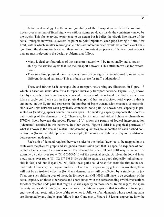
These and further basic concepts about transport networking are illustrated in Figure 1-3which is based on actual data for a European inter-city transport network. Figure 1-3(a) showsthe physical sets of transmission spans present. It is spans of this network that fail when we pos-tulate a cable cut. Each span in the physical graph (a) has an associated total capacity that isannotated on the figure and represents the number of basic transmission channels or transmis-sion layer links between each physically connected node pair. As shown here, capacity is pre-sented as (working, spare) couplet on each span. The working capacity supports the shortest-path routing of the demands in (b). These are, for instance, individual lightwave channels onDWDM fibers between the nodes. Figure 1-3(b) shows the pattern of logical interconnection(“demand”) required in this network. In other words, Figure 1-3(b) is a graphical portrayal ofwhat is known as the demand matrix. The demand quantities are annotated on each dashed con-nection in (b) and would represent, for example, the number of lightpaths required end-to-endbetween each node pair.
Each unit of demand required between nodes in the logical layer has to be mapped onto aroute over the physical graph and assigned a transmission path that is a specific sequence of con-nected channels over the chosen route. The demand between N1 and N10 may be served forexample by paths over route (N1-N2-N3-N10) of the physical graph. But from the logical layerview, paths over route (N1-N2-N7-N6-N10) would be equally as good (logically indistinguish-able in fact) and thus if span (N2-N3) fails, these paths could be shifted from the first to the sec-ond route. However, the diagram makes it clear that if a span in (a) gets cut in isolation, therewill not be an isolated effect in (b). Many demand pairs will be affected by a single cut in (a).Thus, any such shifting over of the paths for node pair (N1-N10) will have to be cognizant of theactual capacity on those other spans and coordinated with the corresponding switchover actionsfor other affected node pairs that might also use capacity on those spans. In this regard, the sparecapacity values shown in (a) are reservations of additional capacity that is sufficient to supportend-to-end path restoration (one of the schemes to follow) of all demands whose working pathsare disrupted by any single-span failure in (a). Conversely, Figure 1-3 lets us appreciate how the
Grover.book Page 21 Sunday, July 20, 2003 3:46 PM
22 Chapter 1 • Orientation to Transport Networks and Technology
available capacity on the edges of graph (a) can be cross-connected in different ways to supportdifferent patterns of demand in (b). This is also the conceptual point about transport networksthat Figure 1-2 is conveying.
The two network views, logical and physical, in Figure 1-3 also convey two basic classesof problem, depending on whether capacities or demands are assumed as given quantities. Oneclass of problem assumes that a forecast or planning view of the demand pattern is given. Thismay actually be a family of possible future demand patterns, or, a stipulated “envelope” of max-imum anticipated demands that the network may have to serve. The problem then is to solve forthe minimum cost allocation of transmission capacity in (a) (or addition of new capacity to anexisting set of capacities) that supports both the routing and protection of all demands in (b).Once a network is built, however, the nearer-term operational problem is one of routing andconfiguring protection arrangement so that demands that actually arrive are both served and pro-tected within the current as-built capacity. Over the life of a network these two phases are revis-ited in a constant cycle.
Unlike circuit switching for voice, the lifetime of connections in the transport network isgenerally much longer, typically days to years because the aggregations of traffic do not changeas rapidly as individual service connections do. For this reason, transport network connectionsare often referred to as “semi-permanent” or “nailed-up” connections. The routing environmentis also different from routing through networks of trunk groups. First, in making rearrangementswithin the transport network (especially for restoration) there essentially cannot be any block-ing, because “blocking” in the transport domain means hard outage for all the services that the
Figure 1-3 A physical transport network and overlying pattern of service layer demand.
(a) A physical transmission network with work-ing (and spare) capacity on spans
(b) A logical pattern of interconnection, or virtual topology, implemented (and protected) over (a)
Grover.book Page 22 Sunday, July 20, 2003 3:46 PM
23
blocked carrier signal would have borne. Secondly, once established, paths in the transport net-work may be very long-lived so there is much more impetus to try to globally optimize theassignment of transport capacity. In contrast, the routing of any one call only commits the sys-tem for a few minutes, after which time the system gets to start over with subsequent calls. Inother words, the system state rapidly decorrelates in the voice circuit-switched network (or thestate of flows in an IP router-based network) but has a much longer correlation time in the trans-port network.
1.0.3 Multiplexing and SwitchingMultiplexing is the simultaneous transmission of many separate messages or lower-speed
logical circuit connections over a shared medium.2 Multiplexing can be via space, time, fre-quency or code division. Space refers to parallel physically distinct channels, such as the sepa-rate fibers of a fiber optic cable or physically separate output ports on a switch or router. Timerefers to synchronous time slot allocation, as in SONET, or asynchronous time slot allocation asin ATM. Frequency division multiplexing (FDM) is the basis for conventional AM/FM radioand the pre-fiber generation of high capacity analog and digital microwave transmission sys-tems. When applied to optical frequencies, FDM is the basis of both coarse and dense wave-length division multiplexing (WDM).
There are two basic types of switching that may be used in transport networks: packetswitching and circuit switching. In a packet-switched network, the information flowing fromone node to another is broken down into sequences of packets at the sending node before beingtransmitted over the network to the receiving node(s). When a packet arrives at a switchingnode, it waits in a queue to be transmitted over the next transmission facility en route to its des-tination. At the receiving node, the packets are reassembled to reconstruct the original informa-tion stream. Because the packets occupy the full capacity on a transmission facility only for theirduration, the transmission capacity can be shared over time with many other connections (or ses-sions). This is referred to as statistical multiplexing. Statistical multiplexing takes advantage ofthe strong law of large numbers to obtain efficiency in bandwidth use. In this context, the princi-ple states that for a number of independent flows, the bandwidth necessary to satisfy the needsfor all of the flows together stays nearly constant, and much less than the sum of their individualpeak rates, even though the amount of traffic in individual flows can vary greatly. Intuitively,the averaging effect is easy to appreciate, especially when delay can be introduced through abuffer to queue up the access to the transmission link. At any moment a few applications couldbe increasing their traffic while other applications are reducing their traffic. The larger the num-ber of sources, the more that individual uncorrelated changes balance each other out to approxi-mate a near-constant total bandwidth requirement. If a large amount of queuing delay is used,the constant bandwidth approaches the overall average rate of all sources. In contrast with TDM
2. This section, through to Section 1.2.3, is adapted with permission from the tutorial portions of the Ph.D. thesis by D. Morley [Morl01].
Grover.book Page 23 Sunday, July 20, 2003 3:46 PM
24 Chapter 1 • Orientation to Transport Networks and Technology
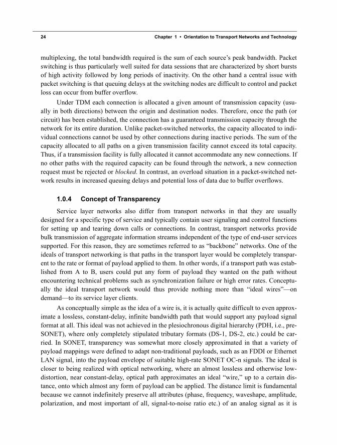
multiplexing, the total bandwidth required is the sum of each source’s peak bandwidth. Packetswitching is thus particularly well suited for data sessions that are characterized by short burstsof high activity followed by long periods of inactivity. On the other hand a central issue withpacket switching is that queuing delays at the switching nodes are difficult to control and packetloss can occur from buffer overflow.
Under TDM each connection is allocated a given amount of transmission capacity (usu-ally in both directions) between the origin and destination nodes. Therefore, once the path (orcircuit) has been established, the connection has a guaranteed transmission capacity through thenetwork for its entire duration. Unlike packet-switched networks, the capacity allocated to indi-vidual connections cannot be used by other connections during inactive periods. The sum of thecapacity allocated to all paths on a given transmission facility cannot exceed its total capacity.Thus, if a transmission facility is fully allocated it cannot accommodate any new connections. Ifno other paths with the required capacity can be found through the network, a new connectionrequest must be rejected or blocked. In contrast, an overload situation in a packet-switched net-work results in increased queuing delays and potential loss of data due to buffer overflows.
1.0.4 Concept of Transparency
Service layer networks also differ from transport networks in that they are usuallydesigned for a specific type of service and typically contain user signaling and control functionsfor setting up and tearing down calls or connections. In contrast, transport networks providebulk transmission of aggregate information streams independent of the type of end-user servicessupported. For this reason, they are sometimes referred to as “backbone” networks. One of theideals of transport networking is that paths in the transport layer would be completely transpar-ent to the rate or format of payload applied to them. In other words, if a transport path was estab-lished from A to B, users could put any form of payload they wanted on the path withoutencountering technical problems such as synchronization failure or high error rates. Conceptu-ally the ideal transport network would thus provide nothing more than “ideal wires”—ondemand—to its service layer clients.
As conceptually simple as the idea of a wire is, it is actually quite difficult to even approx-imate a lossless, constant-delay, infinite bandwidth path that would support any payload signalformat at all. This ideal was not achieved in the plesiochronous digital hierarchy (PDH, i.e., pre-SONET), where only completely stipulated tributary formats (DS-1, DS-2, etc.) could be car-ried. In SONET, transparency was somewhat more closely approximated in that a variety ofpayload mappings were defined to adapt non-traditional payloads, such as an FDDI or EthernetLAN signal, into the payload envelope of suitable high-rate SONET OC-n signals. The ideal iscloser to being realized with optical networking, where an almost lossless and otherwise low-distortion, near constant-delay, optical path approximates an ideal “wire,” up to a certain dis-tance, onto which almost any form of payload can be applied. The distance limit is fundamentalbecause we cannot indefinitely preserve all attributes (phase, frequency, waveshape, amplitude,polarization, and most important of all, signal-to-noise ratio etc.) of an analog signal as it is
Grover.book Page 24 Sunday, July 20, 2003 3:46 PM
25
transmitted over an increasing length of fiber and number of optical amplifiers and possiblewavelength-changing transponders. Thus, a more practical notion is that of digital transparency[Dixi03], p.105 where any format or rate of digital payload signal, up to some maximum work-ing bit rate is accommodated. Such digital transparency is being provided by recent develop-ments such as digital wrapper and GFP, that we discuss further in Chapter 2.
1.0.5 Layering and Partitioning
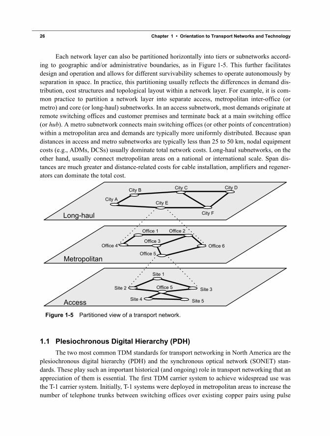
Over many different multiplexing and transmission technologies, the basic routing andswitching functions that they employ are logically equivalent. The main difference is the unit forallocating capacity. In SONET the basic unit of allocation is an STS-n channel, whereas in opti-cal networking it is a wavelength (or to be precise, an optical channel with a specified bandwidthin Hz). There are other important differences but from a functional perspective, these network-ing technologies can be modeled in a generic fashion for many purposes using the same abstractconcepts. This has several implications. First, because the basic functions are equivalent innature, the same types of network elements and architectures are implemented across the rangeof technologies. For example, the survivable ring architectures first implemented in SONET canalso be implemented in the optical network layer. Similarly electronic digital cross-connects(DCS) for SONET remain logically equivalent in many regards to optical cross-connects (OXC)in the optical network layer. The adjacent layers in the network form client-server relationships,in which transport layers perform signal multiplexing, transport and routing for one or more cli-ent layers. For example, the SONET/SDH layer can accept payloads directly from either thePDH, ATM or IP layers. In turn, the resource requirements from the SONET layer become pay-loads for the WDM layer. Figure 1-4 shows most of the currently possible inter-layering trans-port relationships.
IP
ATM
SONET/SDH
WDM
Fibre
PDH
Figure 1-4 Examples of possible client/server associations in a layered transport network.
Grover.book Page 25 Sunday, July 20, 2003 3:46 PM
26 Chapter 1 • Orientation to Transport Networks and Technology
Each network layer can also be partitioned horizontally into tiers or subnetworks accord-ing to geographic and/or administrative boundaries, as in Figure 1-5. This further facilitatesdesign and operation and allows for different survivability schemes to operate autonomously byseparation in space. In practice, this partitioning usually reflects the differences in demand dis-tribution, cost structures and topological layout within a network layer. For example, it is com-mon practice to partition a network layer into separate access, metropolitan inter-office (ormetro) and core (or long-haul) subnetworks. In an access subnetwork, most demands originate atremote switching offices and customer premises and terminate back at a main switching office(or hub). A metro subnetwork connects main switching offices (or other points of concentration)within a metropolitan area and demands are typically more uniformly distributed. Because spandistances in access and metro subnetworks are typically less than 25 to 50 km, nodal equipmentcosts (e.g., ADMs, DCSs) usually dominate total network costs. Long-haul subnetworks, on theother hand, usually connect metropolitan areas on a national or international scale. Span dis-tances are much greater and distance-related costs for cable installation, amplifiers and regener-ators can dominate the total cost.
1.1 Plesiochronous Digital Hierarchy (PDH)The two most common TDM standards for transport networking in North America are the
plesiochronous digital hierarchy (PDH) and the synchronous optical network (SONET) stan-dards. These play such an important historical (and ongoing) role in transport networking that anappreciation of them is essential. The first TDM carrier system to achieve widespread use wasthe T-1 carrier system. Initially, T-1 systems were deployed in metropolitan areas to increase thenumber of telephone trunks between switching offices over existing copper pairs using pulse
Long-haul
Metropolitan
Access
City D
City A
City B City C
City F
City E
Office 2Office 1
Office 4 Office 6Office 5
Office 3
Site 2 Office 5
Site 1
Site 3
Site 4 Site 5
Figure 1-5 Partitioned view of a transport network.
Grover.book Page 26 Sunday, July 20, 2003 3:46 PM
Plesiochronous Digital Hierarchy (PDH) 27
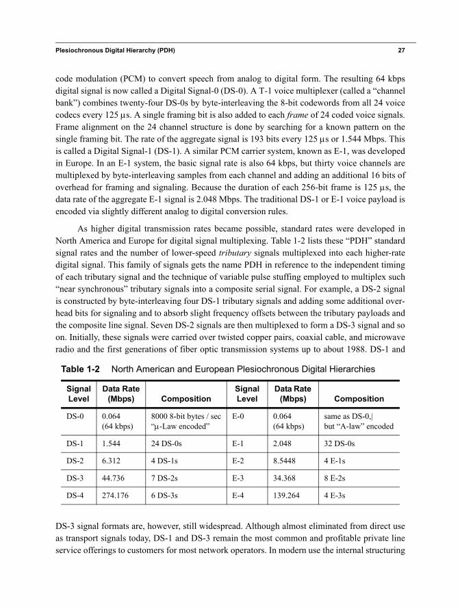
code modulation (PCM) to convert speech from analog to digital form. The resulting 64 kbpsdigital signal is now called a Digital Signal-0 (DS-0). A T-1 voice multiplexer (called a “channelbank”) combines twenty-four DS-0s by byte-interleaving the 8-bit codewords from all 24 voicecodecs every 125 µs. A single framing bit is also added to each frame of 24 coded voice signals.Frame alignment on the 24 channel structure is done by searching for a known pattern on thesingle framing bit. The rate of the aggregate signal is 193 bits every 125 µs or 1.544 Mbps. Thisis called a Digital Signal-1 (DS-1). A similar PCM carrier system, known as E-1, was developedin Europe. In an E-1 system, the basic signal rate is also 64 kbps, but thirty voice channels aremultiplexed by byte-interleaving samples from each channel and adding an additional 16 bits ofoverhead for framing and signaling. Because the duration of each 256-bit frame is 125 µs, thedata rate of the aggregate E-1 signal is 2.048 Mbps. The traditional DS-1 or E-1 voice payload isencoded via slightly different analog to digital conversion rules.
As higher digital transmission rates became possible, standard rates were developed inNorth America and Europe for digital signal multiplexing. Table 1-2 lists these “PDH” standardsignal rates and the number of lower-speed tributary signals multiplexed into each higher-ratedigital signal. This family of signals gets the name PDH in reference to the independent timingof each tributary signal and the technique of variable pulse stuffing employed to multiplex such“near synchronous” tributary signals into a composite serial signal. For example, a DS-2 signalis constructed by byte-interleaving four DS-1 tributary signals and adding some additional over-head bits for signaling and to absorb slight frequency offsets between the tributary payloads andthe composite line signal. Seven DS-2 signals are then multiplexed to form a DS-3 signal and soon. Initially, these signals were carried over twisted copper pairs, coaxial cable, and microwaveradio and the first generations of fiber optic transmission systems up to about 1988. DS-1 and
DS-3 signal formats are, however, still widespread. Although almost eliminated from direct useas transport signals today, DS-1 and DS-3 remain the most common and profitable private lineservice offerings to customers for most network operators. In modern use the internal structuring
Table 1-2 North American and European Plesiochronous Digital Hierarchies
SignalLevel
Data Rate(Mbps) Composition
SignalLevel
Data Rate (Mbps) Composition
DS-0 0.064(64 kbps)
8000 8-bit bytes / sec“µ-Law encoded”
E-0 0.064(64 kbps)
same as DS-0,|but “A-law” encoded
DS-1 1.544 24 DS-0s E-1 2.048 32 DS-0s
DS-2 6.312 4 DS-1s E-2 8.5448 4 E-1s
DS-3 44.736 7 DS-2s E-3 34.368 8 E-2s
DS-4 274.176 6 DS-3s E-4 139.264 4 E-3s
Grover.book Page 27 Sunday, July 20, 2003 3:46 PM
28 Chapter 1 • Orientation to Transport Networks and Technology
of both formats has evolved, however, to support various clear-channel and mixed voice-datauses.
A disadvantage of the pulse-stuffing synchronization scheme used in PDH is that any highspeed signal must be completely demultiplexed to access any of its individual tributary signalsfor add or drop purposes. For example, to drop a DS-1 from a DS-3, the entire DS-3 signal mustundergo two stages of demultiplexing, first to the DS-2 rate and then to the DS-1 rate. Once thedesired signal has been dropped, the remaining DS-1s must be remultiplexed to the DS-3 level.Another limitation is the lack of a uniform set of functions for network performance monitoring,fault detection, provisioning and other network management features and capabilities.
1.2 SONET / SDHJust prior to the advent of SONET standards, systems based on PDH rates and pulse-stuff-
ing multiplexing techniques had reached 12 x DS-3 (Nortel FD-565) and 24 x DS-3 (RockwellLTS-1200) rates. But these systems used signal formats, monitoring methods, modulation tech-niques, laser types, and so on, that were proprietary to each vendor. The emerging “tower ofBabel” above DS-3 rates strongly motivated development of SONET standard by network oper-ators. They wanted SONET to standardize all vendors so that transmitters, receivers, regenera-tors, cross-connects, network controllers, and so on, would all interoperate as separatelypurchased piece-parts. But SONET also reflected accumulated experience with remote monitor-ing and network operations: the philosophy, made possible on fiber, was for SONET to be delib-erately lavish on overheads for monitoring, fault sectionalization, voice orderwire, protectionswitching, remote provisioning, etc., confident that the operational benefits would far outweighany added bandwidth cost.
SONET also provides for direct DS-0 visibility within a high speed multiplex format byusing synchronous byte-oriented multiplexing at all levels of the signal hierarchy. Any tributarysignal in a SONET signal can be accessed without successive demultiplexing steps as in PDH.This requires that all sources of tributary signals must be frequency synchronous. SONET thusrequires precise network-wide frequency synchronization. This is achieved through atomic ref-erence clocks at selected nodes and schemes of phase-locked frequency synchronization in othernodes. Precise time from GPS receivers also aids in maintaining synchronization. The interna-tional version of SONET is the Synchronous Digital Hierarchy (SDH) [ITU96]. SONET / SDHmultiplexing and transmission systems are widely deployed world-wide and evolving to includedata-oriented enhancements covered in Chapter 2.
SONET provides an essentially complete example of all the basic logical elements oftransport networking. That, plus its general pervasiveness in transport networking, are the rea-sons we include a limited overview of the topic as basic background. For more in-depth treat-ments of SONET/SDH, see [Sill96], [SeRe92], [Alle96] or the standards themselves [AN95a]and [AN95b]. Once the basic transport network elements are seen in the context of SONET, thefunctions of their DWDM networking counterparts are fairly easily anticipated, although not yetstandardized. Indeed, recent developments in optical networking, covered in Chapter 2, take on
Grover.book Page 28 Sunday, July 20, 2003 3:46 PM
SONET / SDH 29
increasingly SONET-like attributes as they develop toward practical networking use, becausethe same fundamental problems are faced again. An optical layer cross-connect evolves to bealmost a functional clone of a SONET DCS, for instance. What the DCS did for timeslots, theoptical cross-connect does for lightwave channels, etc. Optical layer rings are similarly almostlogical clones of SONET rings, and so on. SONET, therefore, remains relevant both commer-cially and conceptually as a vehicle for studying the basic logical functions and conceptsinvolved in any transport network.
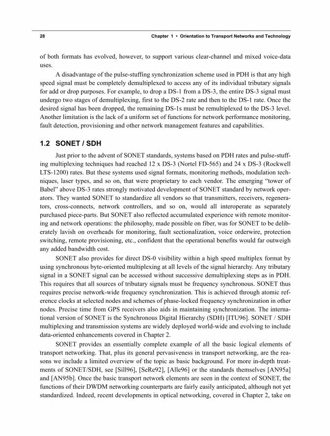
The basic building block in SONET is the synchronous transport signal-level 1 (STS-1).The STS-1 frame provides nine rows by 90 columns of 8-bit bytes as shown in Figure 1-6. TheSTS-1 frame time is 125 µs, reflecting the basic period for sampling speech at 8,000 times a sec-ond. With a total of 810 bytes the STS-1 bit rate is 51.840 Mbps. The STS-1 frame providestransport overhead and a synchronous payload envelope (SPE). The transport overhead occupiesthe first three columns of the frame and is further divided into line and section overheads, thatprovide signal framing, line identification, performance monitoring, and voice and data channels(used for provisioning and maintenance). The SPE occupies the remaining 87 columns by ninerows. The first column of the SPE is used for path overhead functions such as end-to-end perfor-mance monitoring and path identification. The other 86 columns are for payload signals.
An STS-1 SPE can carry a single DS-3 (44.736 Mbps) or it may be subdivided intosmaller envelopes to provide backwards compatibility with lower bit rate PDH signals. Forexample, a DS-1 signal can be carried within an STS-1 SPE by mapping it into a SONET virtualtributary—1.5 (VT1.5). An STS-1 SPE can carry up to 28 VT1.5s. Four VTs are defined inSONET: VT1.5, VT2, VT3, and VT6. They are intended to carry DS1 or E1, DS1C, and DS2payloads, respectively. Each VT has its own overhead bit package, a separate unit within the
3 columns 87 columns
90 columns
9rows
TransportOverhead
Synchronous Payload Envelope (SPE)
3 x 9 bytes(27 bytes)
87 x 9 bytes(783 bytes)
Figure 1-6 The SONET STS-1 frame structure.
Grover.book Page 29 Sunday, July 20, 2003 3:46 PM
30 Chapter 1 • Orientation to Transport Networks and Technology
STS-1 signal. The overhead plus fixed stuffing to permit a fit into the STS-1 frame means theVT1.5 actually has a line rate of 1.728M bps. A VT group carries four VT1.5s, three VT2s, twoVT3s, or one VT6. An STS-1 SPE is filled with seven VT groups, a path overhead, and twovacant columns. VT groups with different types of VTs can be mixed within a single STS-1.This gives the capability to accommodate both the DS-1 signal and the E-1s.
SONET signals at rates that are multiples of the STS-1 rate are obtained by byte-interleav-ing a whole number of STS-1s. Services that require clear-channel multiples of the STS-1 pay-load (for instance an STS-3c for ATM) can be transported by concatenating several STS-1signals together. The resultant signal is designated an STS-Nc. The difference is that an STS-Nis a simple assembly of N intact and separate STS-1s each with its own payload and overheads.The STS-Nc has a single N times payload field and a single overhead stream. Higher rate signalscan be comprised of any combination of lower rate individual STS-1s or concatenated signals.For example, an STS-12 signal can be created from 12 STS-1 signals or 4 STS-3c signals or anyother combination of STS-1 and STS-3c signals that equals STS-12. Prior to transmission, theSTS-N signal is scrambled and converted to a corresponding optical carrier signal (OC-N).Scrambling ensures certain properties for reliable physical layer transmission, such as dc bal-ance and edge transition density for timing recovery. Table 1-3 lists the most commonly usedSONET and SDH signal levels and their transmission rates. SDH standardizes only multiples of
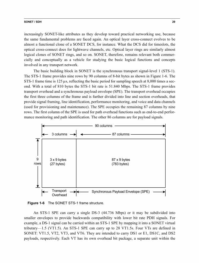
the 155.35 Mb/s rate of the OC-3 SONET signal, and refers to the resulting level as Synchro-nous Transport Modules (STM). SONET’s concatenation ability is important for carrying singlehigh-bit rate streams of Internet Protocol data packets. The “wider” the single pipe that can beprovided, the better the throughput versus delay and statistical multiplexing efficiency is. Thereare some issues, however, in that some large OC-N concatenations, such as OC-48c (~2.5 Gb/s)do not provide very efficient bandwidth matches to the native formats of IP traffic such as Giga-bit Ethernet (GbE). This leads to the technique of virtual concatenation in Chapter 2. Above the
Table 1-3 SONET / SDH Digital Signal Hierarchy
SONET Signal Level Optical Signal
Data Rate (Mb/s)
SDH Equivalent
STS-1 OC-1 51.84 none
STS-3 OC-3 155.25 STM-1
STS-12 OC-12 622.08 STM-4
STS-24 OC-24 1244.16 STM-8
STS-48 OC-48 2488.32 STM-16
STS-192 OC-192 9953.28 STM-64
Grover.book Page 30 Sunday, July 20, 2003 3:46 PM
SONET / SDH 31
top rate of OC-192 defined in the original SONET standards, the industry is developing OC-768(STM-256) systems as well. The corresponding rate of ~40 Gb/s is considered by many to be thehighest serial rate that is technically and economically feasible for electrical processing andswitching. Above this rate recourse is made to separate wavelengths to carry multiple 40 Gb/spayloads, and then to multiple fibers when the feasible number of wavelengths per fiber isreached. Thus, time, frequency and space are all dimensions used for multiplexing to realizetransport capacity requirements.
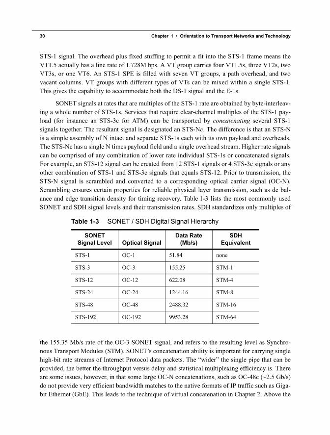
Table 1-4 summarizes some SONET payload mappings that have been so far defined. PoSrefers to Packet-on-SONET. The 10 Gb Ethernet to OC-192c mapping is primarily intended fordirect wavelength transport for wide-area LAN and data-center interconnect applications.
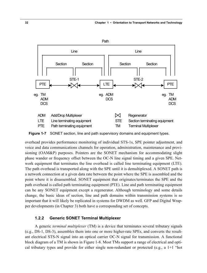
1.2.1 SONET Overheads
The SONET overhead and transport functions are divided into three logical layers ordomains of visibility: section, line and path. The extent of each of these domains is illustrated inFigure 1-7. The section overhead provides framing and performance monitoring for the STS-Nsignal and local voice “order-wire” and data communications channels. Network equipment thatterminates the section overhead is called section terminating equipment (STE). This typicallyincludes regenerators, terminal multiplexers, add/drop multiplexers and digital cross-connectsystems. Regenerators are used at intermediate points along the line to extend transmission dis-tance by converting the optical signal to the electrical domain, retiming and reshaping the STS-N signal and retransmitting it in optical form. Optical amplifiers may also be used betweenregenerators to increase the power level of the optical signal without optical-to-electrical (O/E)conversion and further extend transmission distance. Compared to amplification (where the sig-nals stays in optical domain) regeneration is a much more costly process in general. The line
Table 1-4 Some traditional and non-traditional payloads accommodated by mapping into SONET/SDH containers
Payload SONET Structure Used
10 Gb Ethernet (IP) OC-192c
HDLC / IP (PoS) OC-48 to OC-192
FDDI STS-3c
DS1 SF, DS1 ESF VT 1.5 (28 / STS-1)
DS3 (PDH) STS-1
DS3 (C-bit parity) STS-1
ATM (B-ISDN) STS-3c
Grover.book Page 31 Sunday, July 20, 2003 3:46 PM
32 Chapter 1 • Orientation to Transport Networks and Technology
overhead provides performance monitoring of individual STS-1s, SPE pointer adjustment, andvoice and data communications channels for operation, administration, maintenance and provi-sioning (OAM&P) purposes. Pointers are the SONET mechanism for accommodating slightphase wander or frequency offset between the OC-N line signal timing and a given SPE. Net-work equipment that terminates the line overhead is called line terminating equipment (LTE).The path overhead is transported along with the SPE until it is demultiplexed. A SONET path isa network connection at a given data rate between the point where the SPE is assembled and thepoint where it is disassembled. SONET equipment that originates/terminates the SPE and thepath overhead is called path terminating equipment (PTE). Line and path terminating equipmentcan be any SONET equipment except a regenerator. Although terminology and some detailschange, the basic ideas of section, line and path domains within transmission systems is soimportant that it will likely be replicated in systems for DWDM as well. GFP and Digital Wrap-per developments (in Chapter 3) both have a corresponding set of concepts.
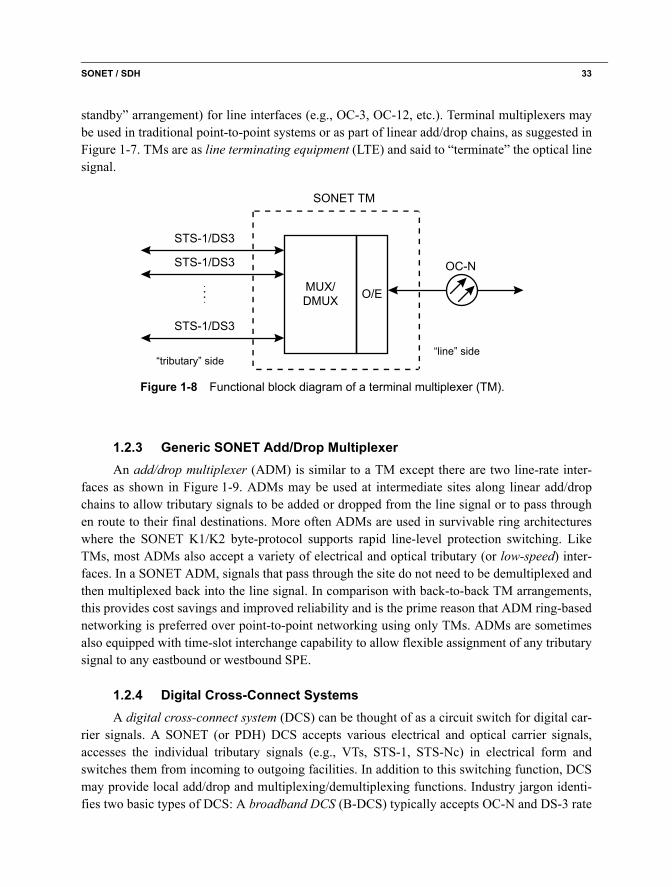
1.2.2 Generic SONET Terminal Multiplexer
A generic terminal multiplexer (TM) is a device that terminates several tributary signals(e.g., DS-1, DS-3), assembles them into one or more higher-rate SPEs, and converts the result-ant electrical STS-N signal into an optical carrier OC-N signal for transmission. A functionalblock diagram of a TM is shown in Figure 1-8. Most TMs support a range of electrical and opti-cal tributary types and provide for either single non-redundant or protected (e.g., a 1+1 “hot
Section Section Section Section
Line Line
Path
RegeneratorADM Add/Drop Multiplexer
TM Terminal Multiplexer
PTE LTE PTE
PTE Path terminating equipmentLTE Line terminating equipment STE Section terminating equipment
STE-1 STE-2
eg. TMADMDCS
eg. ADMDCS
eg. TMADMDCS
Figure 1-7 SONET section, line and path supervisory domains and equipment types.
Grover.book Page 32 Sunday, July 20, 2003 3:46 PM
SONET / SDH 33
standby” arrangement) for line interfaces (e.g., OC-3, OC-12, etc.). Terminal multiplexers maybe used in traditional point-to-point systems or as part of linear add/drop chains, as suggested inFigure 1-7. TMs are as line terminating equipment (LTE) and said to “terminate” the optical linesignal.
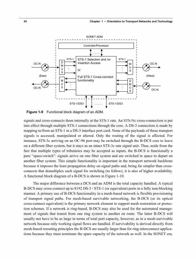
1.2.3 Generic SONET Add/Drop MultiplexerAn add/drop multiplexer (ADM) is similar to a TM except there are two line-rate inter-
faces as shown in Figure 1-9. ADMs may be used at intermediate sites along linear add/dropchains to allow tributary signals to be added or dropped from the line signal or to pass throughen route to their final destinations. More often ADMs are used in survivable ring architectureswhere the SONET K1/K2 byte-protocol supports rapid line-level protection switching. LikeTMs, most ADMs also accept a variety of electrical and optical tributary (or low-speed) inter-faces. In a SONET ADM, signals that pass through the site do not need to be demultiplexed andthen multiplexed back into the line signal. In comparison with back-to-back TM arrangements,this provides cost savings and improved reliability and is the prime reason that ADM ring-basednetworking is preferred over point-to-point networking using only TMs. ADMs are sometimesalso equipped with time-slot interchange capability to allow flexible assignment of any tributarysignal to any eastbound or westbound SPE.
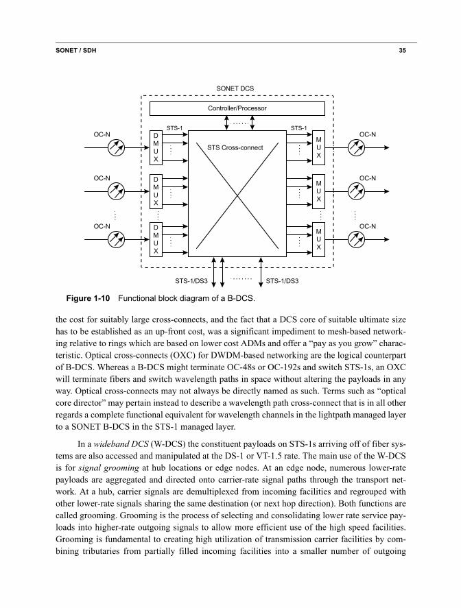
1.2.4 Digital Cross-Connect SystemsA digital cross-connect system (DCS) can be thought of as a circuit switch for digital car-
rier signals. A SONET (or PDH) DCS accepts various electrical and optical carrier signals,accesses the individual tributary signals (e.g., VTs, STS-1, STS-Nc) in electrical form andswitches them from incoming to outgoing facilities. In addition to this switching function, DCSmay provide local add/drop and multiplexing/demultiplexing functions. Industry jargon identi-fies two basic types of DCS: A broadband DCS (B-DCS) typically accepts OC-N and DS-3 rate
SONET TM
STS-1/DS3
OC-N
MUX/DMUX
STS-1/DS3
STS-1/DS3
O/E
Figure 1-8 Functional block diagram of a terminal multiplexer (TM).
“line” side“tributary” side
Grover.book Page 33 Sunday, July 20, 2003 3:46 PM
34 Chapter 1 • Orientation to Transport Networks and Technology
signals and cross-connects them internally at the STS-1 rate. An STS-Nc cross-connection is putinto effect through multiple STS-1 connections through the core. A DS-3 connection is made bymapping to/from an STS-1 in a DS-3 interface port card. None of the payloads of these transportsignals is accessed, manipulated or altered. Only the routing of the signal is affected. Forinstance, STS-3c arriving on an OC-96 port may be switched through the B-DCS core to leaveon a different fiber system, but it stays as an intact STS-3c rate signal unit. Thus, aside from thefact that multiple types of tributaries may be accepted as inputs, the B-DCS is functionally apure “space-switch”: signals arrive on one fiber system and are switched in space to depart onanother fiber system. This simple functionality is important in the transport network backbonebecause it imposes the least propagation delay on signal paths and, being far simpler than cross-connects that demultiplex each signal for switching (to follow), it is also of higher availability.A functional block diagram of a B-DCS is shown in Figure 1-10.
The major difference between a DCS and an ADM is the total capacity handled. A typicalB-DCS may cross-connect up to 8192 DS-3 / STS-1 (or equivalent) ports in a fully non-blockingmanner. A primary use of B-DCS functionality in a mesh-based network is flexible provisioningof transport signal paths. For mesh-based survivable networking, the B-DCS (or its opticalcross-connect equivalent) is the primary network element to support mesh restoration or protec-tion schemes. If a network is ring-based, B-DCS may also be used for the automated manage-ment of signals that transit from one ring system to another en route. The latter B-DCS willusually not have to be as large in terms of total port capacity, however, as in a mesh-survivablenetwork because only working signal flows are handled. If survivability is derived directly frommesh-based rerouting principles the B-DCS are usually larger than for ring-interconnect applica-tions because they must terminate the spare capacity of the network as well. In the SONET era,
DMUX
OC-N
Controller/Processor
SONET ADM
STS-1/DS3 STS-1/DS3
OC-NMUX
STS Cross-connect
(East) (West)
STS-1 STS-1
MUXOC-N OC-N
DMUX
Figure 1-9 Functional block diagram of an ADM.
STS-1 Selection and /or Insertion Access
or
Full STS-1 Cross-connect functionality
Grover.book Page 34 Sunday, July 20, 2003 3:46 PM
SONET / SDH 35
the cost for suitably large cross-connects, and the fact that a DCS core of suitable ultimate sizehas to be established as an up-front cost, was a significant impediment to mesh-based network-ing relative to rings which are based on lower cost ADMs and offer a “pay as you grow” charac-teristic. Optical cross-connects (OXC) for DWDM-based networking are the logical counterpartof B-DCS. Whereas a B-DCS might terminate OC-48s or OC-192s and switch STS-1s, an OXCwill terminate fibers and switch wavelength paths in space without altering the payloads in anyway. Optical cross-connects may not always be directly named as such. Terms such as “opticalcore director” may pertain instead to describe a wavelength path cross-connect that is in all otherregards a complete functional equivalent for wavelength channels in the lightpath managed layerto a SONET B-DCS in the STS-1 managed layer.
In a wideband DCS (W-DCS) the constituent payloads on STS-1s arriving off of fiber sys-tems are also accessed and manipulated at the DS-1 or VT-1.5 rate. The main use of the W-DCSis for signal grooming at hub locations or edge nodes. At an edge node, numerous lower-ratepayloads are aggregated and directed onto carrier-rate signal paths through the transport net-work. At a hub, carrier signals are demultiplexed from incoming facilities and regrouped withother lower-rate signals sharing the same destination (or next hop direction). Both functions arecalled grooming. Grooming is the process of selecting and consolidating lower rate service pay-loads into higher-rate outgoing signals to allow more efficient use of the high speed facilities.Grooming is fundamental to creating high utilization of transmission carrier facilities by com-bining tributaries from partially filled incoming facilities into a smaller number of outgoing
DMUX
DMUX
DMUX
STS Cross-connect
OC-N
OC-N
OC-N
Controller/Processor
SONET DCS
STS-1/DS3 STS-1/DS3
OC-N
OC-N
OC-N
MUX
MUX
MUX
STS-1 STS-1
Figure 1-10 Functional block diagram of a B-DCS.
Grover.book Page 35 Sunday, July 20, 2003 3:46 PM
36 Chapter 1 • Orientation to Transport Networks and Technology
facilities. Grooming may also be done to collect together signals of a common type for enhancedservice management or monitoring and to support multiple classes of service by segregatingdemand by service type, destination or protection category. The W-DCS functionality may bestandalone or part of a multi-service provisioning platforms (MSPP) that will interface a largerange of signal types, both voice and data, and both groom and multiplex these payloads onto asingle higher-rate carrier such as an OC-48, and launch it onto a corresponding path to its desti-nation over the transport network, or to a hub node for further routing. Note that grooming is inmany ways the circuit-switched counterpart to statistical multiplexing, although without thecongestion implications. When data is being both groomed from typically low utilization accesspipes, and statistically multiplexed to higher utilization levels, the overall process is often called“aggregation.” A typical commercial name for a device that performs the W-DCS function, butadds data aggregation and optical OC-n or GigE output formats would be an “edge director.”
The important overall picture is that regardless of the technology, basic architectural prin-ciples lead to their being two fundamental types of “cross-connect” functionality:
• Edge or hub devices that collect lower speed payloads together based on common routing (or common end destinations) and multiplex up to rates suitable for application to an OC-N path or lightwave path through the transport network. Typically in edge grooming the payloads being multiplexed arrive in lightly-loaded access transmission systems.
• Core or backbone devices that interconnect transmission channels at the OC-N or light-wave channel levels to realize the required transport paths and, in a mesh-survivable net-work, to perform the rerouting functions that protect these paths.
In practice, commercial cross-connect or service management platforms may integratethese two basic functions because almost every node has some local add/drop requirements aswell as serving as a transport level switching point. For more background on DCS functions andrequirements in general, see [Bell88] and for specifics of the role of DCS systems in mesh resto-ration see [Bell93].
1.2.5 Hubs, Grooming and BackhaulAnyone who has taken a trip by air that required them to take a commuter flight to a major
hub airport can relate to the concept of grooming and the related role of a hub node. What theairlines want to do is make sure that their biggest planes fly well-loaded and over the long dis-tances for which they are optimized. It would not be economic, nor provide desired service qual-ity, to have a Boeing 747 land every 100 miles to let a half a dozen people on or off. Aircraft ofthis calibre are used on long-haul routes between major “hubs” on routes for which a suitablenumber of passengers sharing the same destination (or next hub) can be grouped together. Thesmaller commuter planes, often lightly loaded, bring people from many small centers into thehub. Each commuter plane is carrying people with different ultimate destinations. But over allthe commuter arrivals at the hub, everyone who is that day heading to Southeast Asia are
Grover.book Page 36 Sunday, July 20, 2003 3:46 PM
SONET / SDH 37
grouped together for the hop to, say, Hong Kong. The process of collecting together passengersthat can usefully all share the common hop to Tokyo is called grooming in the transport context.In an analogy to communication networks, the lightly loaded commuter planes are the accesssystems, the grouping together of everyone going to S.E. Asia is grooming, the combining into awell-filled 747 is multiplexing (and the 747 itself is a high-capacity transport path).
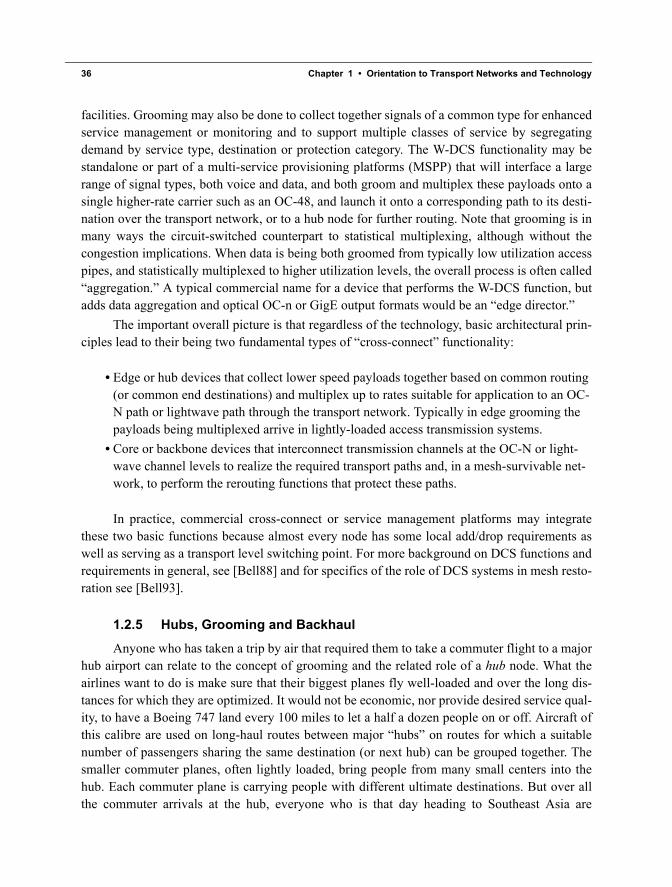
Figure 1-11 illustrates this role of a hub node with a notional W-DCS. In a typical applica-tion the W-DCS may be programmed to pick and choose individual DS1s out of all the incomingDS3s and assemble them into STS-1s that are efficiently filled with co-destined DS1s or DS1sthat all share the need for transport to the same intermediate node in another region. The nodesthat perform this grooming function are called hubs. Hub sites are important factors influencingthe (apparent) demand patterns seen in the logical and system layers and are a consideration inthe design of both ring- and mesh-based survivable networks. With effective grooming, trans-
port signals such as a SONET OC-n, or a wavelength bearing several OC-n, can be efficientlyfilled with lower-speed connections near their points of origin, all of which share a common des-tination or a common intermediate hub. This allows optical (or in general transport-layer)bypass at intermediate nodes with considerable savings in add/drop costs and electronics costs atthose nodes.
Backhaul refers to the process of bringing lower speed signals to the hub site to begroomed into the more efficient long-haul carrier signals leaving the hub. Viewed solely fromthe lower-speed payload standpoint, going to the hub may actually route it away from its ulti-mate destination. Again the airline analogy gives an essentially exact explanation of the process,and the trade-offs involved. One’s individual destination may be Anchorage, Alaska, say. But ifyou want to get there from Edmonton, Canada you are first routed south to Seattle (directlyaway from the destination). The reason is that it is only at the Seattle hub that enough individualtravellers going to Anchorage can be collected from the surrounding region to fill a 767-classplane from Seattle to Anchorage at a suitably high fill factor. The backhaul is illustrated by the
Figure 1-11 Grooming diverse demands from lightly loaded access facilities into well-filledtransport signals to other regional hubs or destinations.
A B - A- X X - D D - K - A - A - B - BB - Z
A D - - K - Z- D - A - B - B B - - B - X- - - -
Y -B - K - X Z- D - K - A - A - B B B - K- -
W-DCS “grooming”
X X X X K K K K K- Z Z - Z - - - - - - -
B B - - B- BB - B- BBBBB B ... B .B
AA - - A- AAAAAA- AAA A ... A A ..... numerous diversely des-tined low fill access signals....
high fill STS1 direct to B
high fill STS1 direct to A
high fill STS1 to regional hub for nodes X K Z.
Grover.book Page 37 Sunday, July 20, 2003 3:46 PM
38 Chapter 1 • Orientation to Transport Networks and Technology
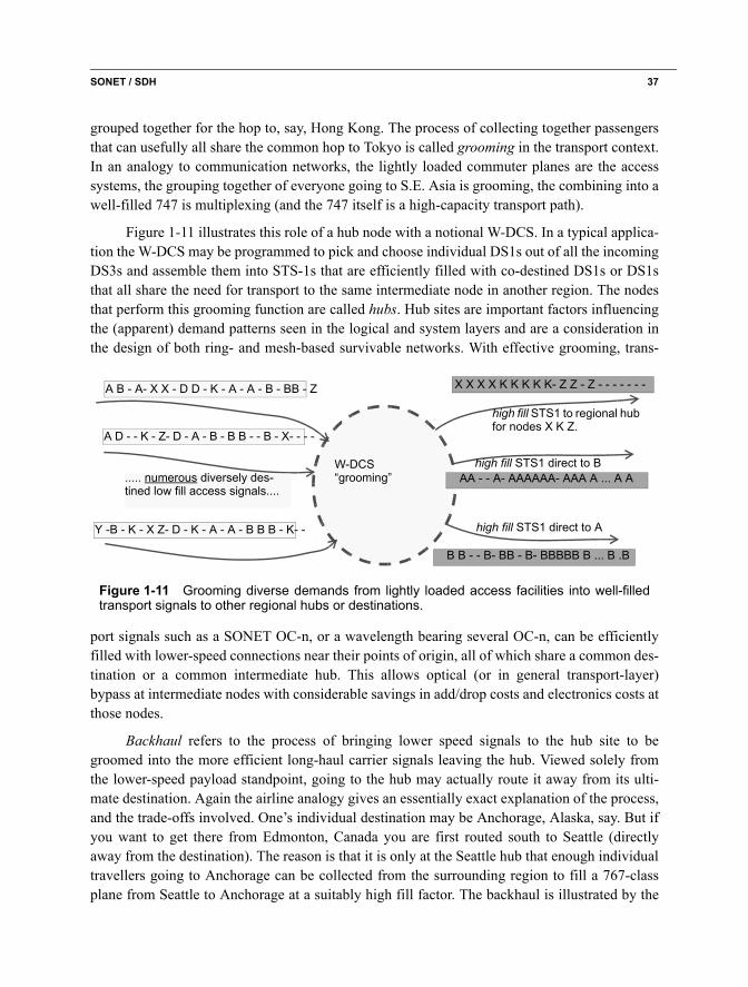
fact that Edmonton is partway north between Anchorage and Seattle, so there is a significantbackhaul component in this routing. The identical concepts explain why an individual DS-1 maybe routed on a lightly loaded regional DS-3 via a path involving a backhaul over local accesstransmission systems to a hub where it may then join an entire OC-48 going to its destination (orto another hub in the destination region). The corresponding view of how access regions, hubs,and backbone transport are interrelated in a network as a whole is illustrated in Figure 1-12.
Historically, the practice seems to have been one of establishing cross-connect hubs at thelargest regional central offices. Once such hubs are given, grooming has been primarily treatedas the problem of finding aggregations of lower-speed signals that can economically justifyestablishment of certain larger outgoing high speed signal containers to each other hub. Eachsuch establishment decision is made independently. Typically, 60 to 75% fill is a criteria thatturns out to be economic for establishing a new high-speed signal to a corresponding hub. If suf-ficient traffic cannot be aggregated to justify a direct higher-speed connection from the currentnode, the lower-speed signals are routed indirectly via another hub that must handle them againat their lower speed. In a future optical mesh network there is considerable research still to bedone on globally optimized strategies of hub placement for access-grooming, backhaul routing,and optical bypass savings.
To appreciate the issues and tie into this related research, see [ZhMu02], [ZhBi03],[MoLi01] and [SiSu00] (p.286). In this book we consider problems of survivable transportdesign where the set of high speed signal path requirements is already determined as outputfrom the grooming decision process. In reality, however, details of the transport layer designdetermine certain costs that will influence the grooming strategy and the grooming decisionsdefine which wavelength paths are needed in the transport layer. This should be kept in mind as
Figure 1-12 Concepts of access, hubs, grooming, backhaul, and transport. (source: [FrSo01 ])
Hundreds of accessnodes
Tens of backbone nodes
Access regions in which back-haul, grooming, and multiplexing occurs
Grover.book Page 38 Sunday, July 20, 2003 3:46 PM
Broadband ISDN and Asynchronous Transfer Mode (ATM) 39
the methods of this book may be iteratively solved in conjunction with grooming methodsdeveloped elsewhere to approximate a joint optimization of both grooming and transport archi-tectures.
1.2.6 Fundamental Efficiency of Edge Grooming and Core TransportThe three basic functions of edge-grooming, hub-grooming, and core cross-connection are
in a sense fundamental specializations that are bound to emerge under almost any technology.SONET recognizes it with B-DCS and W-DCS generic elements. IP (and ATM) data network-ing reflects the specializations of edge and core routers and under MPLS (to follow) we findwith label edge routers (LERs) and label switching routers (LSRs). In optical networking, simi-lar distinctions between access and core optical switches are also emerging. But the concept oftransport networking, the fundamental efficiency it offers, and the fact that it emerges in allother real-world contexts involving transportation is not completely accepted in telecommunica-tions, perhaps because “disruptive” technologies come so frequently. A tendency is for majoradvances in switching or routing technology to be coupled with proposed network architecturesthat would, in our prior analogy, amount to landing the 747 every 100 km to add and drop a fewpassengers. ATM switches to handle every cell of OC-192s, terabit IP packet switches, and opti-cal packet switching are examples. The general point is that it is fundamentally unnecessary andunadvantageous to ever handle every cell, packet, or call at every core switching node. Anydevice that can handle every transiting packet or cell, at a node will inevitably require morespace, power, complexity, cost and maintenance than a corresponding transport node handlingonly containers, coupled with a smaller local access node. A well-groomed lightpath routed andprotected in the optical transport layer is ultimately a far more cost-efficient and scalable meansto pass data through a node than to inspect and reroute every packet. The fundamental architec-ture of access, grooming and transport will therefore always offer efficiency and cost advantagesas long as there are any limits to router (or switch) speed, power, space, cost, or reliability.
1.3 Broadband ISDN and Asynchronous Transfer Mode (ATM)The Broadband Integrated Services Digital Network (BISDN) was developed to support
demand-switched, semipermanent, and permanent broadband connections for both point-to-point and point-to-multipoint applications. Channels operating at STS-3c and OC-12 were seenas the main bearer channels for BISDN. The foundation of BISDN is the label-switched routingof fixed-size Asynchronous Transfer Mode (ATM) cells using SONET/SDH transport.
BISDN was a precursor to the Internet in its intent, but IP-based applications and network-ing have supplanted it. The main legacy of BISDN / ATM, however, is the proven concepts ofvirtual circuits and label switching, which are now the basis of MPLS for IP traffic. BISDN rec-ognized that compared to operating several dedicated networks, network service integration canprovide advantages in terms of economics, implementation, operation, and maintenance. Whilededicated networks require several distinct subscriber access lines, BISDN access can be basedon a single optical fiber. A variety of interactive broadband services can be supported with
Grover.book Page 39 Sunday, July 20, 2003 3:46 PM
40 Chapter 1 • Orientation to Transport Networks and Technology
BISDN: broadband video telephony; corporate videoconferencing; video surveillance; high-speed digital transport of medical images, artwork, and advertising; high-speed clear-channeldata transmission; file transfer; high-resolution fax; color fax; video retrieval; TV distribution;LAN interconnection, etc.
Instead of reserving time slots as in STM networks, information in ATM is packetized andplaced in short 53-byte cells that are multiplexed and transmitted asynchronously on the trans-mission medium. The 53 bytes of an ATM cell consist of a 48-byte information field and a 5-byte header. Two of the fields defined in the header are the Virtual Path Identifier (VPI) and theVirtual Circuit Identifier (VCI). VPI is a 12-bit field and the VCI is a 16-bit field that togetherdefine the routing information of a cell. As with any other packet-switching network, routing ofcells is performed at every node for each arriving cell. ATM can support a variety of services(e.g., telephone, image, video and data), with a guaranteed Quality of Service (QoS). A VirtualCircuit Connection (VCC) in ATM is analogous to a virtual circuit in data networks, such as anX.25 or a frame relay logical connection. The VCC is the basic unit of switching in ATM net-works. For ATM, a second tier of labeling defines a virtual path. A Virtual Path Connection(VPC) is a bundle of VCCs that have the same endpoints, e.g., switching systems, LAN gate-ways, etc. Thus, cells flowing over all of the VCCs in a single VPC may be switched together.Because VP switching is inherently more efficient than VC switching, it is advantageous toswitch a cell in a VP. This Virtual Path concept was developed in response to a trend in high-speed networking in which the control cost of the network is becoming increasingly high in pro-portion to the overall network costs. The Virtual Path technique helps reduce the control cost bygrouping connections sharing common paths through the network into a single unit. Networkmanagement actions can then be applied to a small number of groups of connections instead of alarge number of individual connections.
For more detail on ATM, readers are referred to [Onvu94] and the first five chapters of[WuNo97]. The last two chapters of [WuNo97] describe ATM VP-based protection switchingmechanisms, although without an emphasis on network design. We return to ATM VP-basedprotection switching mechanisms as the starting point in Chapter 7, which develops networkdesign for controlled oversubscription of capacity upon restoration in ATM or MPLS networks.
1.4 Concept of Label-Switching: The Basis of ATM and MPLSATM and multi-protocol label switching (MPLS) are both based on “label-switching.” In
ATM, fixed-size cells arrive in one port of an ATM switch and the label they bear in the celloverhead is used to index a routing table at the node that indicates the outgoing port and newlabel number to be assigned to the cell. In MPLS, variable-length IP packets arriving at a label-switching router (LSR) are similarly redirected based on incoming port and label, to a next-hopoutgoing port and new label. In both schemes, a connection setup protocol creates the sequenceof {out-port, next-label} entries along a desired path so that a logical circuit is establishedbetween any desired origin node (and application or user) and destination host (and application).ATM uses the virtual circuit (VC) construct to connect individual application-level connections.
Grover.book Page 40 Sunday, July 20, 2003 3:46 PM
Concept of Label-Switching: The Basis of ATM and MPLS 41
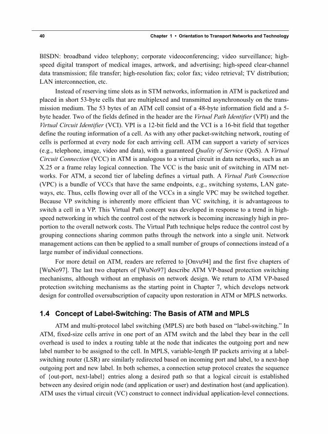
MPLS (over IP) uses logical port numbering schemes to distinguish between packets for differ-ent applications running on the same host or sharing the same label-switched path.
The concept of label-switching is illustrated in Figure 1-13 where two label-switchedpaths are shown. In Figure 1-13(a) node B receives an unlabeled packet (or cell) at the entry tothe path with an indication that its destination is node F. A separate path setup process isassumed to have previously laid down a set of label-swapping rules at each node involved. If theintention is to create the path shown in Figure 1-13(a), then the label swapping entries at eachnode to create this path are shown in the top four rows of Table 1-5. The corresponding entries tocreate the path in Figure 1-13(b) are in the second half of the table. The example defines two dif-ferent paths that could be established between nodes B and F. The example packet initiallyarrives at node B but does not bear a label at that point. We use the label field in the table to indi-cate, however, that its destination is known (node F). At node B, the routing table entry says ineffect “if anything comes in going to node F, send it to node A with a label E.” When node B
E
e
F
F
DE
B C
A
E
e
D
F
Figure 1-13 Examples of label-switched paths.
(a) A label-switched path on the route B-A-E-F
(b) A label-switched path on the route B-C-D-E-F
IP packet
Encapsulated IP packet
Grover.book Page 41 Sunday, July 20, 2003 3:46 PM
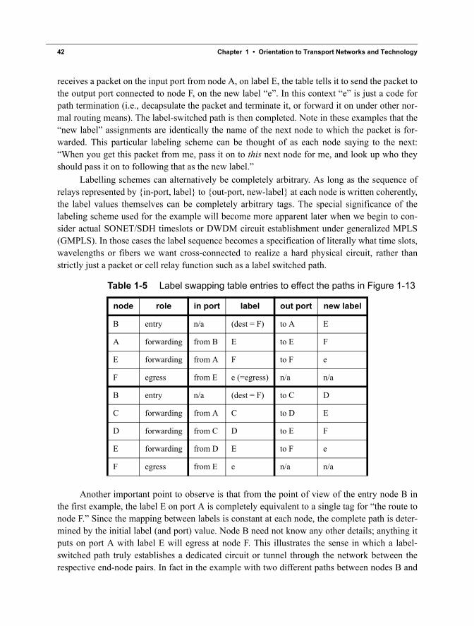
42 Chapter 1 • Orientation to Transport Networks and Technology
receives a packet on the input port from node A, on label E, the table tells it to send the packet tothe output port connected to node F, on the new label “e”. In this context “e” is just a code forpath termination (i.e., decapsulate the packet and terminate it, or forward it on under other nor-mal routing means). The label-switched path is then completed. Note in these examples that the“new label” assignments are identically the name of the next node to which the packet is for-warded. This particular labeling scheme can be thought of as each node saying to the next:“When you get this packet from me, pass it on to this next node for me, and look up who theyshould pass it on to following that as the new label.”
Labelling schemes can alternatively be completely arbitrary. As long as the sequence ofrelays represented by {in-port, label} to {out-port, new-label} at each node is written coherently,the label values themselves can be completely arbitrary tags. The special significance of thelabeling scheme used for the example will become more apparent later when we begin to con-sider actual SONET/SDH timeslots or DWDM circuit establishment under generalized MPLS(GMPLS). In those cases the label sequence becomes a specification of literally what time slots,wavelengths or fibers we want cross-connected to realize a hard physical circuit, rather thanstrictly just a packet or cell relay function such as a label switched path.
Another important point to observe is that from the point of view of the entry node B inthe first example, the label E on port A is completely equivalent to a single tag for “the route tonode F.” Since the mapping between labels is constant at each node, the complete path is deter-mined by the initial label (and port) value. Node B need not know any other details; anything itputs on port A with label E will egress at node F. This illustrates the sense in which a label-switched path truly establishes a dedicated circuit or tunnel through the network between therespective end-node pairs. In fact in the example with two different paths between nodes B and
Table 1-5 Label swapping table entries to effect the paths in Figure 1-13
node role in port label out port new label
B entry n/a (dest = F) to A E
A forwarding from B E to E F
E forwarding from A F to F e
F egress from E e (=egress) n/a n/a
B entry n/a (dest = F) to C D
C forwarding from A C to D E
D forwarding from C D to E F
E forwarding from D E to F e
F egress from E e n/a n/a
Grover.book Page 42 Sunday, July 20, 2003 3:46 PM
Concept of Label-Switching: The Basis of ATM and MPLS 43
F, node B could consider that it has two separate permanent circuits that it can use to send trafficto node F: route 1 = {port A, label E}, route 2 = {port C, label D}. A pair of such virtual circuitsor label-switched paths can be used in practice for load balancing over the two routes, or as aform of protection switching.
Label-switching was adopted for both ATM and MPLS out of a fundamental need for acircuit-like logical construct for many networking purposes. Pure datagram flows cannot be con-trolled enough to support QoS assurances and effective and fast schemes for restoration aregreatly enabled by the manipulation of either physical or logical circuit-like quantities, ratherthan redirection of every single packet or cell through conventional IP routing tables. The reasonfailure recovery is faster within a circuit-oriented paradigm is ultimately the same reason thatbasic delay, throughput and loss rates of cell or packet transport are improved by switching asopposed to routing.
Routing involves determining a next-hop decision at every node based on the absolute glo-bal destination (and sometimes source and packet type) information of the packet in conjunctionwith globally-determined routing tables at each node. This is fundamentally a more time-con-suming and unreliable process than label-switching. A conventional IP router has to perform amaximum length address-matching algorithm on every packet and rely on continual topologyupdates to ensure a correct routing table entry for every possible destination IP address in theadministrative area. The maximal length aspect of the address-matching refers to the fact that apacket’s destination address may produce no exact match in the routing table. In such cases thepacket is forwarded toward the subnetwork with the maximal partial address match.
In label switching, however, the next hop decision is made with entirely local informationestablished previously in an explicit connection setup process. The local information is the labelswapping tables in an LSR, or simply the physical connection state between input and outputtimeslots or wavelengths in a cross-connect. In a physical fiber or metallic switch, or in atimeslot-changing switch, or a wavelength cross-connect, the switching information (i.e., theoutport and next timeslot or wavelength) is stored in the physical connection state. In an LSR orATM switch, the forwarding port and next-label are stored in tables that are typically muchsmaller than a full IP routing table, and operate on the basis of an exact label match which is fun-damentally much faster, autonomous, and reliable than IP datagram routing.
1.4.1 Multi-Protocol Label Switching (MPLS)In MPLS, a relatively short “label” replaces the full interpretation of an IP packet's header
as necessary under conventional forwarding. In traditional IP forwarding, packets are processedon the basis of the global destination address at every router along the path. This is also knownas hop-by-hop routing. In contrast, MPLS encapsulates IP packets with a label when the packetfirst arrives into an MPLS routing domain. The MPLS edge router will look at the information inthe IP header and select an appropriate label for it. The label selected by the MPLS edge routercan be based on QoS and explicit routing considerations, not just the destination address in theIP header. This is in contrast to conventional IP routing, where the destination address will
Grover.book Page 43 Sunday, July 20, 2003 3:46 PM
44 Chapter 1 • Orientation to Transport Networks and Technology
determine the next hop for the packet. All subsequent routers in the MPLS domain will then for-ward the packet based on the label, not the IP header information. Then, as the labeled packetsexit the MPLS domain, the edge router through which it is leaving will remove the label. Thevalue of the label usually changes at each LSR in the path as the incoming label is looked up andswapped for another. Thus labels only have meaning between neighboring nodes. With this,MPLS can be used to forward data between neighboring nodes even if no other nodes on the net-work support MPLS.
MPLS uses two categories of label-based routers: label edge routers (LERs) and labelswitching routers (LSRs). An LSR is used in the core of an MPLS network and participates inthe establishment of LSPs and high-speed switching of flows over existing LSPs. Notably manyLSRs are implemented with high capacity ATM label-switching switch hardware as their corewith a conventional router added to participate in the LSP establishment protocol and to performrouting functions for the residual traffic of a normal IP datagram nature (i.e., packet traffic thatdoes not constitute significant flows per se to warrant establishment of an LSP). The LER sup-ports access to the MPLS core network. Edge routers are classified as either ingress or egress.An MPLS ingress router performs the initial routing lookup and LSP assignment for launchingthe packets into the fabric of logical pipes through the MPLS core. The egress LER removeslabels and performs a further routing table lookup to continue the packet on its way under con-ventional routing. LERs can have many types of access interface (frame relay, ATM, Ethernetfor example).
MPLS allows a packet flow to be fully “routed” only once, at the entry to an IP network,and thereafter label-switched all the way to its egress router. Aside from the fact that the packetflows remain asynchronous and statistically multiplexed, in all logical regards, once the IP pack-ets for that destination are encapsulated with a label and put in the appropriate outgoing queuefrom the egress node, it is like they have been dropped into a dedicated pipe or tunnel direct tothe destination. The train of switching relationships written in the label-swapping tables en routecreates a hard-wired sequence of relays that is fully amenable to hardware implementation ateach node, and referred to as a Label Switched Path (LSP). This improves router networkthroughput and delay performance compared to routing every packet at every node en routebased on its ultimate destination IP address.
In assigning IP packets to LSPs, an LER makes use of the concept of forwarding equiva-lence. A Forwarding Equivalence Class (FEC) is a set of IP destination addresses that, from thestandpoint of the given entry node all share the same local routing decision. In conventional IPforwarding, each router needs to maintain FEC tables to indicate for each output port the set ofIP destination addresses that should be sent out that port. In MPLS the FEC tables need be keptonly at LERs and record for each IP address what LSP to put it on (i.e., what initial label andoutgoing port to assign it to). FECs at the LERs are based on class of service requirements andon IP address. The table at the LER that lists the initial label, and outgoing port for each FEC iscalled its label information base (LIB).
Grover.book Page 44 Sunday, July 20, 2003 3:46 PM
Network Planning Aspects of Transport Networks 45
For more detailed background on MPLS the book by Davie and Reckhter [DaRe00], andreferences therein, are suggested. The relevance here is twofold. In Chapter 2 we see how MPLSis extended into Generalized MPLS (GMPLS), with applications in the automatic provisioningof service paths through a transport network at any level such as DS-1 through to whole light-paths. As with ATM, MPLS is also a transport technique that involves circuit-oriented logicalconstructs for the transport of stochastic packet flows, and hence is also amenable to the con-trolled oversubscription design strategy of Chapter 7.
1.5 Network Planning Aspects of Transport Networks
1.5.1 Modularity and Economy-of-ScaleSONET provides an example of a hierarchy of standard rates and formats on which multi-
plexing and transmission system products can be based. Some industry experts expect that anSDH-like progression (4, 16, 64…) of wavelengths per fiber may also arise for DWDM trans-mission. The adoption of a discrete set of modular capacities aids both users and system design-ers. It allows specific technology choices (such as frequency spacing, carrier generation, EDFAnoise, gain, bandwidth, etc.) to be combined and optimized to realize a product offering at eachprice-performance point that the market needs. Some vendors may specialize in the market for16-λ systems while another may use quite different technology to specialize in, say, 768-λ sys-tems. As a result, the actual installed capacity in a SONET (or an optical network as well) isinevitably modular in nature. The relevance to network design is that although we may oftencompare design approaches on the basis of total unit-capacity requirements, we have to keep inmind that the real capacities and costs will be stair-step functions of cost versus capacity. More-over, cost is rarely in linear dependence on the capacity; so there is an economy of scale effect.In detailed studies it can be important to consider the modular and nonlinear cost structure of theactual equipment to be specified. As an example, consider a bidirectional 48-λ DWDM system.The cost structure will reflect all the following physical items: 3
a. One fiber pair and pro-rated cost of right-of-way acquisition, duct and cable, instal-lation, and repeater/amplifier housing costs
b. 48 electrical (transmit) channel interfacesc. Generation and modulation of 48 optical carriersd. Optical WDM multiplexore. In-line optical amplifiers with bandwidth and power capabilities suitable for 48
wavelengths, every 60 to 100 km typicallyf. An average distance-amortized cost for 48 regenerators, every 300 km, sayg. Optical WDM demultiplexorh. 48 electrical (receive) channel interfaces
3. This discussion is adapted for use here from [DoGr00].
Grover.book Page 45 Sunday, July 20, 2003 3:46 PM
46 Chapter 1 • Orientation to Transport Networks and Technology
i. Redundant common power, maintenance processor, rack, cabling, and equipment bay installation costs
Items (a), (d), (e), (g), (i), and a large part of (f), are one-time costs required for the sys-tem’s existence, even if just one channel is operated. Such “get started” cost items are tradition-ally called the “common equipment” in telecommunications and are a major contributor to thenonlinear cost structure. To turn up the first channel, all the common equipment must be present.In principle, all subsequent electrical and optical per-channel circuit packs can then be provi-sioned on a one-by-one basis as needed, but if growth is high or on-demand path establishmentis desired, then all of these may also be preprovisioned. In the limit of full preprovisioning thereis a large step in cost to establish the system, but no further cost depending on how many chan-nels are actually in use. This is the modularity aspect. The economy of scale aspect is that, in thisexample, a 192-λ system may be only two or three times the cost of the 48-λ system (not fourtimes).
If the per-channel costs are actually equipped only on an as-needed basis, then we actuallyhave two levels of capacity-cost modularity. Say for example that for current working require-ments a given facility requires 37 wavelength channels. Then the common equipment for a stan-dard 48-λ system may be required, but only 37 of the per-channel costs need actually beincurred. Thus the cost structure for transport capacity actually has a least two scales on which itis modular. A third sense in which capacity cost is extremely modular is if we recognize the“get-started” cost of having the facility right-of-way in the first place. This is usually only a fac-tor in considering topology design itself, however.
There are several cases where modeling a single scale of modularity can be justified, how-ever, corresponding to the full capacity of each basic module size. First, if the growth rate ishigh and the cost of dispatching maintenance crews to populate new channel cards one-by-one isalso high, then it may make more sense to fully equip the system when installed. Secondly, tosupport truly dynamic path provisioning the systems may be fully preprovisioned wheninstalled. Additionally, in any case where the average system utilization is high following someplanning design study, then the “fully equipped” model also tends to be justified in its own right.Another way to limit the complexity to a single modularity scale while recognizing only partialchannel equipping is to approximate the average fill factor of transmission systems and lump thetotal per-channel costs of this average fill level into the module cost.
A notation used to represent economy of scale is “N times Y times.” For instance 3x2xmeans that a tripling of capacity results in a doubling of cost. “3x2x” is fairly characteristic ofmature SONET transmission technology over the OC-24 to OC-192 range. Similar or evenstronger economy of scale effects may characterize mature DWDM transmission systems.
1.5.2 Fiber Route StructuresIn transport network planning we refer to the fiber route structure on which physical facil-
ities can be built as the network graph. This is the actual set of right-of-ways on which permis-
Grover.book Page 46 Sunday, July 20, 2003 3:46 PM
Network Planning Aspects of Transport Networks 47
sion to lay fiber cables is in hand. Several recently built networks are based on rights-of-wayobtained from a cooperating, co-owned or defunct power, gas, or railway utility and so inheritsome of the topological properties of those networks. Typical transport network graphs tend tohave an irregular mesh interconnection pattern with an average number of geographicallydiverse rights-of-ways at junction sites that varys from two to at most about seven at any indi-vidual node. This measure of nodal route-diversity is called the span-degree or just the “degree”of a node. The corresponding average over all nodes is also referred to as the network averagenodal degree, .
In some North American networks may be as low as 2.3, indicating a quite sparse topol-ogy. A degree of two at every node is the minimum possible in any network that has a fullyrestorable topology. In contrast some European networks have as high as 4.5. Figure 1-14allows visualization of these two extremes, using examples from published data on real net-works. Note, however, that even the most richly connected transport graphs are quite sparse rel-ative to truly random graphs of full mesh graphs. Transport network graphs tend to look neitherlike fully connected networks nor like random graphs where any node may with equal probabil-ity be connected to any other. In addition to the characteristic in the range of 2 - 4.5 real net-works tend to show a high “locality” in that nodes tend to be connected to other nodes that arenear them in the plane. Related to this locality characteristic is planarity. Typical transportgraphs are often strictly planar or have only a few non-planar spans. (Planarity is treated furtherin Chapter 4.) Metropolitan area networks in both North America and Europe tend to be similarto the more richly connected European national backbone example in Figure 1-14(b), whereaslong-haul networks in North America tend to be the most sparse. In contrast to the service layernetworks realized over the transport network, the transport graph is typically much sparser.Sometimes statements about nodal degree cause confusion because the reference is to differentlayers. For instance, viewed at the STS-3c connectivity layer, a given location might logicallyhave a degree of 160. But the same node could be a degree-2 site in the facilities graph. Unlessexplicitly stated otherwise in this book, the default understanding about any reference to the net-work graph or to a nodal degree, we are referring to the physical layer facilities graph.
1.5.3 Network Redundancy
Another important characteristic of transport network and a measure of architectural effi-ciency for a survivable transport network is its redundancy. Redundancy is always a consider-ation in conjunction with survivability design because it indicates how “lean” or efficient thedesign is in its use of spare capacity. Redundancy is in a broad sense the price one has to pay toachieve a target level of restorability or other measures of survivability. Capacity efficiency isdefined as the reciprocal of the redundancy. It is ultimately cost that matters and this is notalways directly proportional to capacity-efficiency, however. High redundancy in ring-basedmetro networks does not always mean they are economically inferior to a less redundant meshnetwork design, for example, because nodal costs may be lower with ring ADMs than with meshcross-connects. But what is always true is that to serve and protect a common base of demands,
d
d
d
d
Grover.book Page 47 Sunday, July 20, 2003 3:46 PM
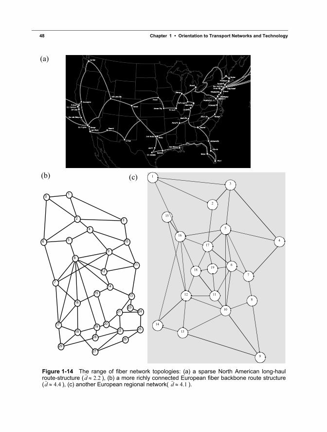
48 Chapter 1 • Orientation to Transport Networks and Technology
0 1
2 3
4
56
7
9
10
1112
13
14
15
16
17
1819
20
2324
25
26
27
28
29
8
21
22
Figure 1-14 The range of fiber network topologies: (a) a sparse North American long-haulroute-structure ( ), (b) a more richly connected European fiber backbone route structure( ), (c) another European regional network( ).
d 2.2≈d 4.4≈ d 4.1≈
(a)
(b) 1
2
3
4
5
6
7
8
9
10
1112
13
14
15
16
17
1819
(c)
Grover.book Page 48 Sunday, July 20, 2003 3:46 PM
Network Planning Aspects of Transport Networks 49
where all other factors are the same, a more redundant design requires more capacity and hencedoes cost more. Especially in long-haul networks, cost does correlate with capacity.
Often in research or basic comparative planning studies, exact cost data is also not avail-able, so redundancy is used as a surrogate for cost in comparing alternatives and as an intrinsicmeasure of network design efficiency. It should also be noted that although redundancy is usu-ally computed from capacity quantities, each unit of capacity on a span has related nodal equip-ment at its ends that is either a per-channel cost to start with or is a common cost that can be pro-rated to each channel of capacity. So redundancy is perhaps the single most generic surrogatethat we have for actual cost effectiveness of an overall survivable network design.
The logical redundancy of a network is defined as the pure ratio of spare to working chan-nel counts and does not take any distance effects into account.
(1.2)
where S is the set of spans in the network, wm is the number of units of working capacity on spanm and sm is the corresponding number of spare capacity units on span m. Spare capacity may bethe protection fibers of APS or ring systems or designed-in spare channels for restoration in amesh network. Note that the definition of redundancy that we use differs from the other possibledefinition which is the ratio of spare to total capacity present, i.e., spare / (working + spare). It issometimes important to clarify which definition of redundancy is being used. The geographicalredundancy is of the same form as Equation 1.2 but each sm, wm term is weighted by a coeffi-cient representing either the distance of a span or the cost per channel on the span.
Both of these redundancy measures are somewhat idealized in that they allow workingand spare capacities to be present in any assumed quantity. But as discussed, the capacities ofreal transmission systems are modular. In such cases the modular redundancy is defined as:
(1.3)
where Cm is the total installed (modular) capacity on span m. In some contexts the non-workingcapacity of modules on a span is sometimes viewed as containing two sub-parts:
where om is called the provisioning overhead due to modularity. The mod-ular geographic redundancy follows the same pattern as above: it is given by Equation 1.3respectively, but every capacity term is again weighted with the distance or cost of span m.
Note that when using redundancy as a figure of merit for comparison of survivability tech-niques, it is only meaningful to compare alternatives in which the working demands are routedin an identical, or at least capacity-equivalent, way. In many problems this is the case becausedemands follow shortest paths in all alternatives and the only comparative questions are aboutthe spare capacity design to protect such working flows. (These are later called “non-joint”design problems and redundancy is always a meaningful comparative measure.) In cases wherethe working routes and working capacity may be manipulated or altered as well as spare capac-ity as part of the overall design strategy, the simple redundancy measures above can be mislead-ing. The reason is that if one increases working route lengths, more total capacity may be
ℜ sm wmm S∈∑⁄
m S∈∑≡
ℜmod Cm wm–( ) wmm S∈∑⁄
m S∈∑≡
Cm wm–( ) sm om+=
Grover.book Page 49 Sunday, July 20, 2003 3:46 PM
50 Chapter 1 • Orientation to Transport Networks and Technology
required, but it will appear that redundancy per se is lower. For this reason the standard redun-dancy of a network is also defined as:
(1.4)
where is the total working capacity needed to support shortest-path routing of alldemands (i.e., the minimum possible working capacity of a network) and is the actualamount of working capacity used to support working paths in the network. Any excess of work-ing capacity above the minimum for shortest path routing is thus equivalent to additional sparecapacity used in the design. This allows meaningful comparison between more general designstrategies (later called “jointly” optimized designs). Under standard redundancy measures anytwo designs serving the same demands on the same graph can be fairly compared.
1.5.4 Shared-Risk Entities and Fault Multiplication Generally, network operators who own and operate their own physical facilities (“facili-
ties-based operators”) pay considerable attention to the physical separation or “diversity” ofcable routings. Particular efforts are made to ensure that important backbone fiber cables arerouted over physically disjoint ducts, pole lines, or buried trenches, or at least on opposite sidesof the same streets. The point is to mitigate the impact that any one physical structure failuremight have in terms of the number of transmission paths it brings down. It is tempting to thinkthat this is a new concern only associated with recent emphasis on automatic network-levelrerouting for survivability. Physical cable diversity has, however, been a general historical con-cern. In some senses diversity was even more important without an embedded network restora-tion mechanism because the outage would last as long as the cable repairs. Care would be takenthen that important services, backbone transmission paths, and key trunk groups would be splitand routed over diverse physical cable or microwave routes. Telephone central office buildingstypically have two to four separate underground cable vault entry points on opposite sides or allcompass points of the building footprint, precisely for diversity.
In more recent practice, where spare capacity is explicitly designed into the network forsurvivability, it is important to take the existence of any “shared risk entities” into account in thecapacity design. A shared risk group (SRG) or shared risk link group (SRLG) defines a set oftransport channels or paths that have something in common: they all fail together if a certain sin-gle item of physical equipment fails [StCh01] [LiYa02] [SeYa01]. The most common ways inwhich multiple different paths share a risk of simultaneous disruption from a single commonphysical failure are:
1. The paths share the same cable (or fiber if on WDM carriers). 2. The paths traverse separate cables that share a common duct or other structure such as a
bridge crossing. 3. The paths are routed through a common node.
ℜ* wm sm+( ) w*mm S∈∑–
m S∈∑
w*mm S∈∑⁄=
w*m∑wm∑
Grover.book Page 50 Sunday, July 20, 2003 3:46 PM
Network Planning Aspects of Transport Networks 51
That paths should share the same cables extensively throughout the network is inevitableand expected. But in certain types of path protection, the set of end-to-end paths that share eachcable must be grouped together for failure planning purposes. Such groups of paths are calledshared risk link groups (SRLGs). The importance to path restoration schemes is that each SRLGthat exists defines a specific set of end-to-end path failures that must be simultaneously restored.More generally any failure of a cable, a duct, or a node defines a set of network paths that aresimultaneously disrupted. Each such physical element failure defines another SRLG. The SRLGconcept is thus the most encompassing category of shared risk failure scenarios. In practice,because single cable cuts are still the most frequent failure event, the set of end-to-end pathsaffected by single cable cuts is also called the “default set of SRLGs.”
Another class of restoration schemes are span-oriented, however, and do not need to con-sider or know the end-to-end details of all the paths affected, because these schemes recoverfrom the failure by replacement routing directly between the end nodes of the failed span (i.e.,the nodes adjacent to a failed span or node). In this context, isolated but complete failure of anindividual cable span connecting adjacent nodes is the basic single-fault model. The aspect ofshared risk that is of concern under span-oriented restoration moves up from planning orientedon individual links within paths to planning that is oriented to shared risk between cables thatdefine the spans between cross-connect nodes. We refer to these as shared risk span groups(SRSGs). Whereas SRLGs are strictly quite numerous (because each cable segment defines atleast one SRLG), there may be many fewer SRSGs in a network because each SRSG representsan unintended lapse in physical layer cable or duct diversity. In other words, an SRSG is a situa-tion where entire cable spans that are at least notionally separate are actually routed togetherover some common structure. This is different than the routine and numerous forms of sharedrisk between all end-to-end paths that traverse the same cable together. The classic case of anSRSG is that of a bridge crossing near a node that is common to two spans. All of the transmis-sion channels in both spans share a common risk of failure on the bridge crossing, although tonetwork planners the logical view may be of two separate cables, for which survivability plan-ning would normally consider only as separate individual failure scenarios. This type of physicallayer diversity lapse may be relatively rare, but the importance of an SRSG in network planningis that it allows for the simultaneous failure of what are otherwise nominally independent spansof the transport graph. In other words, an SRSG sets up a situation where one physical failurecan multiply into two or more logical span failures.
But certain fault multiplication effects can also arise without involvement of an SRSG.Figure 1-15 illustrates a true SRSG on the left, and a nodal bypass arrangement, often referred toas express routes or glass-throughs, on the right. The nodal bypass sets up a particular type logi-cal dual-failure situation. In the nodal bypass one or more paths bypasses node B but follows thesame ducts as other channels on spans A-B and B-C. Such bypass arrangements are usuallyestablished when the demand (in the example, between nodes A and C) warrants its own dedi-cated fiber(s) but a separate geographical route is not available. In this case the A-C expressfibers can be well enough loaded that they can be dedicated to the A-C direct logical span, sav-
Grover.book Page 51 Sunday, July 20, 2003 3:46 PM
52 Chapter 1 • Orientation to Transport Networks and Technology
ing OEO termination costs at the intermediate node B. But this sets up certain logical dual fail-ure situations. For instance, if duct A-B is cut, spans A-B and A-C appear to fail simultaneously.
Perhaps because it might be considered sensitive data, or because it is hard for the networkoperator to determine, it is difficult to obtain network models that are complete with data onSRLGs. Getting rid of span SRLGs has been a historical preoccupation of network plannersregardless of the survivability strategy because SRLGs inherently complicate and undermineany scheme for protection or restoration, even manual patch recovery or 1+1 APS. It is anembarrassment when it is found out (now and then) that some ultra-important service such as aDefense Department backbone link, planned on a diverse 1+1 basis, in fact shares the samebridge crossing (for example) at some unexpected locale in the middle of the country. An inter-esting anecdote is about a pair of “mission critical” telemetry links used to monitor high pres-sure gas pipelines in the Canadian North. For 3,000 km these 1+1 redundant signal paths wereindeed physically diverse and created at considerable expense to establish and audit the pathrealization. The story goes, however, that after some years of operation it was discovered that100 meters from the company operations center in a city 3,000 km to the south both signal feedscrossed a bridge together. So the problem of SRLGs is not new, although the term is recent. Theissue has existed for decades and has traditionally haunted special-services efforts to establish1+1 APS arrangements with confidence in the intended diversity in the physical layer. Evenwhen operators lease carrier services from other service providers to try and assure diversity,
A
B
C
logical intent
actual routing
cables
actual routing for A-C logical link
cable
cable
Figure 1-15 Shared risk span group in the physical layer and closely related concept of phys-ical-to-logical fault escalation.
(a) An SRSG: Two nominally disjoint fiber cables share the same duct or other common physical structure (such as a bridge crossing).
(b) Physical to logical fault multiplication: If physical span B-C is cut, all paths crossing B-C and A-C will fail simultaneously due to the physical layer routing used to realize the logical layer A-C link.
A
B
C
logical A-C link
Grover.book Page 52 Sunday, July 20, 2003 3:46 PM
Network Planning Aspects of Transport Networks 53
SRLGs can manifest themselves. An outcome from Hurricane Hugo in the US was the apparentdiscovery that up to five different network operators had transport spans crossing one particular,seemingly unimportant, small bridge in the rural southwest. This SRLG was discovered whenthe bridge was washed out by the flood surge!
The effect of SRSGs and the logical dual failure scenarios that arise from bypass are bothstudied in further in Chapter 8. In Chapter 3 the related but more general concept of dependentedges is discussedin terms of its implications for the choice of level —physical, logical, or ser-vices layer—at which various survivability principles can be applied.
1.5.5 Demand Patterns We previously described how various service layer traffic types are combined into stan-
dard “demand units” for delivery via the transport network. Thus, different service layer archi-tectures and traffic handling strategies influence the pattern of demand requirements seen by thetransport network. When many nodes have a strong demand flow to (from is always implied aswell) one or two specific nodes the pattern is described as a “hub-like” demand pattern. In a met-ropolitan network this propensity can arise when telephony traffic from many sites is trunked tojust one or two major centers for switching. In addition there may be only one or two toll-con-necting offices to access the long-distance switching network from each metro area. Within themetro area network it therefore appears that there is a strong demand to these “hub nodes.” Theestablishment of regional hubs for grooming also causes a hub-like demand pattern to arise frombringing many DS-3 or STS-1 access connections back to a W-DCS for grooming into well-filled OC-48s (for example) for long haul transport. In the limiting case, this leads to the notionof a perfectly hubbed demand pattern in which all nodes of a region exchange demands onlywith the hub site(s).
As illustrated in Figure 1-12, such hub sites represent each region on the backbone inter-regional transport network. At this level the regional hub sites are typically exchanging demandat the OC-48 or OC-192 level in a much more uniform random mesh-like pattern. In practice,there may be detailed historical, demographic and economic explanations for the exact amountof demand exchanged between each regional hub node, but the overall effect is that of an essen-tially random distribution of demands on each node pair. The random mesh type of demand pat-tern may also arise in dense metropolitan area networks where the community of interestbetween all nodes is essentially almost equal and a hubbing architecture is not used. Callers andother forms of communication from each node are as likely to go to one node as any other in therest of the network.
A historically recognized effect for long haul demand is referred to as a “gravity-like”inverse-distance effect on demand intensities. The intensity of voice communication in particu-lar depends proportionately on the size of the two centers and (at least historically) inversely onthe distance between population centers. There is a classic anecdote of the Severn Bridge inEngland that illustrates this tendency. The Severn Bridge was a major construction effort to spana large estuary that previously separated two cities. The effect of the bridge was to reduce the
Grover.book Page 53 Sunday, July 20, 2003 3:46 PM
54 Chapter 1 • Orientation to Transport Networks and Technology
travel distance between the two communities from hundreds of miles to only a few. Telephonecalling volumes between these centres went up markedly after the bridge was built, givingexperimental evidence for the inverse-distance effect when all other factors were equal. Whenthe bridge brought the two nodes closer together, their mutual attraction (and hence mutual traf-fic) rose more than proportionately.
Of course, any real situation will reflect the individual historical and demographic circum-stances affecting demand. In general, there will always be some blend of uniform, hubbing, andgravity type effects in a real demand pattern seen at the transport layer. Recognition of thesethree constituent pattern types can allow us to numerically model and systematically varydemand patterns for a variety of purposes in network planning or research studies.
Numerical Modeling of Demand Patterns Often network planning or researchstudies have to be conducted without the luxury of a known or reliably forecast demand matrix.Obtaining accurate forecasts of the real demand is a whole discipline of its own. In other con-texts, however, one is conducting comparative network planning or research studies and needsonly a representative demand model on which to base comparative design studies. While there isan infinite number of demand patterns that could be tested, the practical researcher or plannerhas to use only a few test-case demand patterns to try to reach generally true comparative con-clusions about alternatives. A variety of different test-case demand patterns can be made upfrom the following models:
1. Pure logical mesh with equal number of demands on all node pairs2. Random distributed demand: uniform random number of demands on each pair3. Hub-like demand pattern4. Dual hub demand pattern5. Mutual attraction demand models6. “Gravity” demand (mutual attraction with inverse distance dependency)7. Weighted superpositions of the above component patterns
The first two models are self explanatory. The hub and dual hub patterns often character-ize metro or regional area networks involving one or two main hub sites. In general, the demandbetween a hub and a non-hub node may also be inversely proportional to the distance betweenthem. All other node pairs (i.e., between two non-hub nodes) exchange either a constant or uni-form random number of demand units. A numerical model that can be used is:
(1.5)
(1.6)
where d0 and l0 are demand and distance scale constants, respectively, and li,hub is the distancefrom node i to the respective hub, di,hub is the (integer) number of demands generated. The sec-ond part of the model generates a constant mutual demand between all other non-hub nodes.
di hub, int d0 round li hub,( ) l0⁄[ ]–( )=
di non, hub– d1=
Grover.book Page 54 Sunday, July 20, 2003 3:46 PM
Network Planning Aspects of Transport Networks 55
A principle that is believed to underlie real traffic intensities at long-distance scales is theconcept of mutual attraction, independent of distance. For example, New York City and LosAngeles are two of the most important centers in the U.S. New York City also exchanges trafficwith Ottawa, but it is lower because of Ottawa’s lower population and economic status com-pared to Los Angeles. Population data can be one measure of this notion of importance in thereal world, but to generate test-case demand patterns with the same overall characteristics,“importance factors” can be assigned to nodes at random. Another approach is to view nodaldegree as a surrogate for the presumed demographic importance. The argument is that large cen-ters will tend to have higher nodal degree. In either case, once the “importance factors” Ii areassigned to each node i, the mutual attraction demand model is:
. (1.7)
The pure mutual attraction model is independent of distance between centers. The “grav-ity” demand model adds an inverse distance dependency, partially offsetting the mutual impor-tance effect. For example, extending our prior example to include Paris, we might agree thatParis, New York and Los Angeles are all of the same “importance” class, but “distance” (includ-ing geographical, cultural, time-zone offset, etc.) tends to attenuate the Los Angeles–Parisdemand relative to the Los Angeles–New York demand. The fully general “gravity” model pro-duces a number of demands for each (i,j) node pair that responds to both importance and dis-tance as follows:
(1.8)
where α is an exponent modeling the inverse-distance effect and d0 is a scaling constant set sothat the individual demand quantities are in the range intended. Of course the name “gravity”suggests α = 2. But in practice where this method has been compared to actual demand patterns,α much closer to one (e.g., 1.1 to 1.3) have been typically found to be more accurate.
There is evidence that as IP data volumes outpace voice, demand in real backbone net-works is tending even more toward distance independence (i.e., ). This may also be due inpart to flat-rate (distance independent) voice calling plans. A 2001 study of North Americanlong-haul demand evolution showed that pair-wise total demand between nodes was almostuncorrelated to geographical distance. This can be seen in Figure 1-16(a). In a sense, with theInternet, all points are now an insignificant “distance” apart from a social or commercial stand-point. This gives increasing justification for network planning studies to use a distance indepen-dent demand model.
An implication of distance-independent demand is that most traffic at backbone networknodes tends to be transiting traffic. To illustrate, Figure 1-16(b) shows the distribution of physi-cal span distances between adjacent (i.e., directly connected) nodes in the same network towhich the data of Figure 1-16(a) pertain. Together Figure 1-16(a) and (b) imply that in the aver-age backbone node, 70% of the flow at a node transits the site. On average only 30% originates(or terminates) at a node. (This is another compelling argument for the role of cross-connects in
di j, int Ii Ij⋅( ) d0⋅( )=
di j, intIi Ij⋅
Li j,( )α---------------- d0⋅
=
α 0→
Grover.book Page 55 Sunday, July 20, 2003 3:46 PM
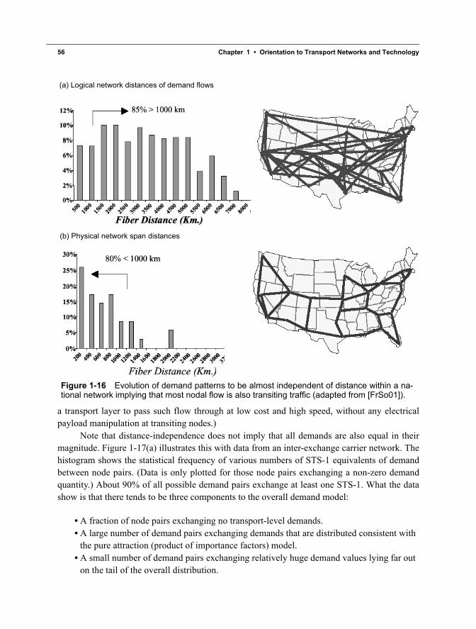
56 Chapter 1 • Orientation to Transport Networks and Technology
a transport layer to pass such flow through at low cost and high speed, without any electricalpayload manipulation at transiting nodes.)
Note that distance-independence does not imply that all demands are also equal in theirmagnitude. Figure 1-17(a) illustrates this with data from an inter-exchange carrier network. Thehistogram shows the statistical frequency of various numbers of STS-1 equivalents of demandbetween node pairs. (Data is only plotted for those node pairs exchanging a non-zero demandquantity.) About 90% of all possible demand pairs exchange at least one STS-1. What the datashow is that there tends to be three components to the overall demand model:
• A fraction of node pairs exchanging no transport-level demands.• A large number of demand pairs exchanging demands that are distributed consistent with
the pure attraction (product of importance factors) model. • A small number of demand pairs exchanging relatively huge demand values lying far out
on the tail of the overall distribution.
(b) Physical network span distances
Figure 1-16 Evolution of demand patterns to be almost independent of distance within a na-tional network implying that most nodal flow is also transiting traffic (adapted from [FrSo01]).
(a) Logical network distances of demand flows
Grover.book Page 56 Sunday, July 20, 2003 3:46 PM
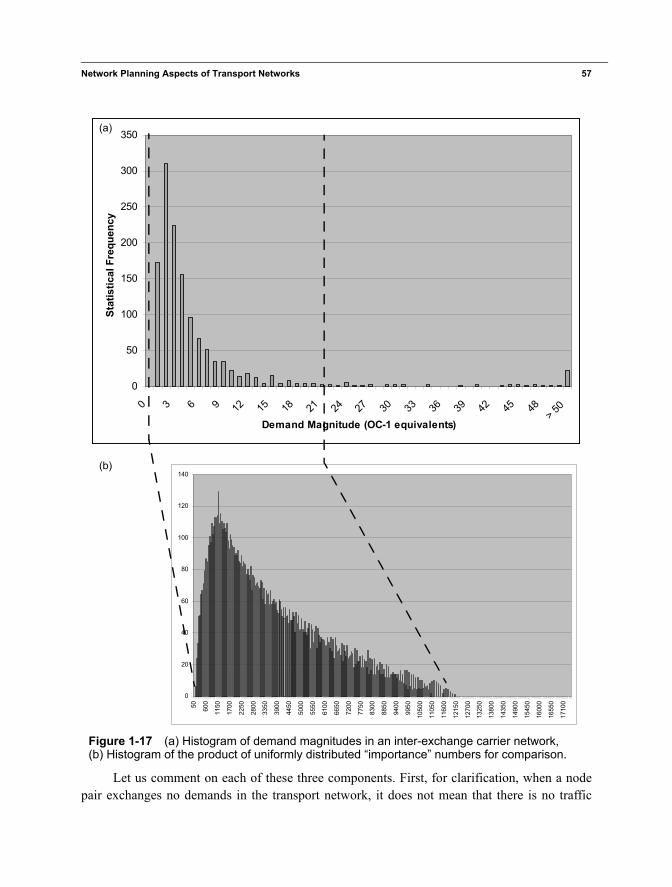
Network Planning Aspects of Transport Networks 57
Let us comment on each of these three components. First, for clarification, when a nodepair exchanges no demands in the transport network, it does not mean that there is no traffic
0
20
40
60
80
100
120
140
50 600
1150
1700
2250
2800
3350
3900
4450
5000
5550
6100
6650
7200
7750
8300
8850
9400
9950
1050
0
1105
0
1160
0
1215
0
1270
0
1325
0
1380
0
1435
0
1490
0
1545
0
1600
0
1655
0
1710
0
Figure 1-17 (a) Histogram of demand magnitudes in an inter-exchange carrier network, (b) Histogram of the product of uniformly distributed “importance” numbers for comparison.
0
50
100
150
200
250
300
350
0 3 6 9 12 15 18 21 24 27 30 33 36 39 42 45 48> 5
0
Demand Magnitude (OC-1 equivalents)
Stat
istic
al F
requ
ency
(a)
(b)
Grover.book Page 57 Sunday, July 20, 2003 3:46 PM
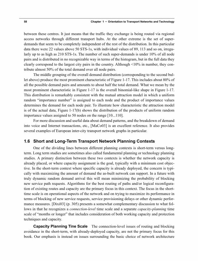
58 Chapter 1 • Orientation to Transport Networks and Technology
between these centres. It just means that the traffic they exchange is being routed via regionalaccess networks through different transport hubs. At the other extreme is the set of super-demands that seem to be completely independent of the rest of the distribution. In this particulardata there were 22 values above 50 STS-1s, with individual values of 89, 113 and so on, irregu-larly up to as high as 210 STS-1s. The number of such super-demands is under 10% of all nodepairs and is distributed in no recognizable way in terms of the histogram, but in the full data theyclearly correspond to the largest city pairs in the country. Although <10% in number, they con-tribute almost 50% of the total demand over all node pairs.
The middle grouping of the overall demand distribution (corresponding to the second bul-let above) produce the most prominent characteristic of Figure 1-17. This includes about 80% ofall the possible demand pairs and amounts to about half the total demand. What we mean by themost prominent characteristic in Figure 1-17 is the overall binomial-like shape in Figure 1-17.This distribution is remarkably consistent with the mutual attraction model in which a uniformrandom “importance number” is assigned to each node and the product of importance valuesdetermines the demand for each node pair. To illustrate how characteristic the attraction modelis of the actual data, Figure 1-17(b) shows the distribution of the products of uniform randomimportance values assigned to 50 nodes on the range [10...110].
For more discussion and useful data about demand patterns, and the breakdown of demandinto voice and Internet transactions, etc., [MaCo03] is an excellent reference. It also providesseveral examples of European inter-city transport network graphs in particular.
1.6 Short and Long-Term Transport Network Planning ContextsOne of the dividing lines between different planning contexts is short-term versus long-
term. Long term studies are sometimes also called fundamental planning or technology planningstudies. A primary distinction between these two contexts is whether the network capacity isalready placed, or where capacity assignment is the goal, typically with a minimum cost objec-tive. In the short-term context where specific capacity is already deployed, the concern is typi-cally with maximizing the amount of demand the as-built network can support. In a future withtruly dynamic random demand arrival this will mean minimizing the probability of blockingnew service path requests. Algorithms for the best routing of paths and/or logical reconfigura-tion of existing routes and capacity are the primary focus in this context. The focus in the short-time scale is on operational aspects of the network and on trying to maximize its performance interms of blocking of new service requests, service provisioning delays or other dynamic perfor-mance measures. [Dixi03] (p. 305) presents a somewhat complementary discussion to what fol-lows in that he recognizes a connection-level time scale and a separate capacity-planning timescale of “months or longer” that includes consideration of both working capacity and protectiontechniques and capacity.
Capacity Planning Tine Scale The connection-level issues of routing and blockingavoidance in the short-term, with already-deployed capacity, are not the primary focus for thisbook. Our emphasis is instead on issues surrounding the basic choice of network architecture
Grover.book Page 58 Sunday, July 20, 2003 3:46 PM
Short and Long-Term Transport Network Planning Contexts 59
and different basic survivability principles and strategies that are options for long term planning.This is the context of fundamental network planning or technology and basic network architec-ture selection studies. These questions are often focused on some form of cost or resource mini-mization to satisfy a forecast demand. It is accepted that the forecast on which different basicarchitectures and strategies are compared will probably be in error. But what will be more last-ing is the basic understanding and insights into one architecture or strategy relative to the otheroptions. Table 1-6 recognizes these two essentially different planning time-scales and indicatessome of the important differences.
Connection Level Time Scale In the short term, network architecture and capacitiesare given. In long term planning, these are basic decisions to be made. In the short term context,the demand may turn out to be different from the forecasts used in long term planning and “cus-tomer churn” is apparent. A kind of limiting case of churn is the notion that lightpath demandsmay come and go as frequently and unpredictably as individual telephone calls. Many recentpapers fall in this category where fixed capacities apply and simulation is used to model block-ing probabilities under various lightpath routing and protection schemes where lightpath arrivalsand departures are modeled as independent memoryless Poisson processes. The claim is thatsuch “dynamic demand” studies get away from the assumption of a specific “static demand”matrix. And yet the Poisson arrival processes have static mean values that completely character-ize the demand between node pairs, indirectly assuming just as accurate a forecast as in the staticdemand cases. It is in fact, quite difficult to predict or simulate short-term blocking performanceor to plan the capacity of a network without ultimately requiring some kind of forecast, or atleast a representative demand model accompanied with uncertainty range estimates.
Table 1-6 Comparison of short and long-term planning contexts
Short term(operational)
Long term(planning and design)
Capacities These are given. These are to be decided upon.
Architecture Given To be decided
Demand Models
Random arrivals/departures or slowly varying demand.
A forecast demand matrix, possibly with different representative demand scenarios.
Typical Problems and Goals
Routing to minimize block-ing probabilities and/or rear-rangements to routing and protection capacity configu-ration.
Minimum cost of capacity and equipment to serve forecast demands (or to provide a work-ing capacity envelope within which to support dynamic demand operations).
Channel Assignment
Detailed time-slot or wave-length assignment.
“Capacity only” model assuming full cross-connection.
Grover.book Page 59 Sunday, July 20, 2003 3:46 PM
60 Chapter 1 • Orientation to Transport Networks and Technology
Forecast Uncertainty The increasing inability to forecast accurately, long enoughahead to deploy networks or augment their physical capacity, is a real issue. Modeling demandarrivals as memoryless Poisson processes of known mean intensities is, however, really no moredynamic than planning capacity to static average-demand forecasts. Even in the most dynamicfuture environments, however, demand at the transport level will arise from changes in theaggregation of many smaller traffic flows, even when routers are themselves the source of thelightpath demands. Such demand combinations are not subject to complete decorrelation afterjust a few holding times (which is an implication of ordinary traffic theory), rather they evolvemore slowly. In other words, the envelope of an aggregation of flows is inevitably less dynamicin time than the individual flows being aggregated.
What seems, therefore, to be more useful in the face of forecast uncertainty is a means ofdesigning network capacity to provide for an envelope of operational states in which a vast num-ber of actual demand patterns is accommodated and protected. In the face of evolving demandpatterns that are unpredictable but have considerable correlation times (not completely indepen-dent states every holding time), successive batch provisioning and incremental growth andreconfiguration approaches can be developed to manage the dynamic demand problem. All ofthe design problems treated in later chapters lend themselves to the latter approaches to handlingdynamic demand. In particular, Chapter 5 explains the concept of a working capacity envelope(WCE) and incremental optimal capacity design models to dimension and adapt network capac-ity to support dynamic traffic and unpredictable evolutions of the demand pattern. The WCEoperational concept also applies directly to p-cycle based networks in Chapter 10. Strategies thatattempt in various ways to take forecast uncertainty directly into account in the economic designof a survivable network are essentially in their infancy, but several initial approaches are beingstudied [KeOl03], [LeGr02], [GeAn01].
A final difference between short and long term planning contexts, especially for opticalnetworks—where full wavelength conversion may not be available at every node—is that ofchannel assignment. When actually provisioning a new path, or restoring a path, specific time-slot or wavelength assignments must be given. Except for a few cases in the chapters that follow,we consider the “capacity only” problem, which leaves detailed time slot or wavelength assign-ment as a secondary problem to be solved. The reason for this is that in the long term context,costs and basic architectural efficiencies and other attributes do not depend on the detailed chan-nel assignments, as long as a suitable channel assignment is feasible under the capacity avail-able. This is the case for SONET mesh networking where the B-DCS can assign any STS-1 toany free time slot in an outgoing OC-N. In a lightpath managed optical network the correspond-ing feasibility of wavelength assignment depends on the availability of wavelength conversion.If the optical cross-connects have an electronic core, then a wavelength conversion capability isimplicit and the problem is logically identical to the SONET case. Where all-optical nodes areinvolved we need only assume that each has a small pool of wavelength converters sufficient toreduce any wavelength blocking to low levels.
Grover.book Page 60 Sunday, July 20, 2003 3:46 PM