Embed Size (px)
Citation preview
ORIGAMI-CONSTRUCTIBLE NUMBERS
by
HWA YOUNG LEE
(Under the Direction of Daniel Krashen)
Abstract
In this thesis I present an exposition of origami constructible objects and their
associated algebraic fields I first review the basic definitions and theorems of field
theory that are relevant and discuss the more commonly known straightedge and
compass constructions Next I introduce what origami is and discuss the basic
single-fold operations of origami Using the set of single-fold operations I explain
what it means for an object to be origami-constructible and show how to prove or
disprove the constructibility of some origami objects Finally I present extensions
of origami theory in literature and pose some additional questions for future studies
Index words Field Theory Compass and Straightedge Construction OrigamiConstruction Constructible Numbers
ORIGAMI-CONSTRUCTIBLE NUMBERS
by
HWA YOUNG LEE
BS Ewha Womans University 2004
MEd Ewha Womans University 2009
PhD University of Georgia 2017
A Thesis Submitted to the Graduate Faculty
of The University of Georgia in Partial Fulfillment
of the Requirements for the Degree
MASTER OF ARTS
Athens Georgia
2017
ccopy2017
Hwa Young Lee
All Rights Reserved
ORIGAMI-CONSTRUCTIBLE NUMBERS
by
HWA YOUNG LEE
Major Professor Daniel Krashen
Committee Robert RumelyPete Clark
Electronic Version Approved
Suzanne BarbourDean of the Graduate SchoolThe University of GeorgiaDecember 2017
Acknowledgments
First I would like to thank all the math teachers and students I had and have
Without these people I would not be here I would also like to thank my advisor
and committee members who provided valuable feedback and support Dr Krashen
thank you for your mentorship patience assistance with technology and creativity
that sparked many ideas for this thesis Dr Rumely thank you for all the origami
books you let me borrow and for our chats about origami both were very helpful
Dr Clark thank you for your advisement and support in pursuing this degree and
for happily joining my committee Additionally I would like to thank my family
and friends for their love and support which gave me the strength to continue my
graduate studies Finally I would like to give a special acknowledgement to my dear
friend Irma Stevens who was always willing to give me advice and help when writing
this thesis
iv
Contents
Acknowledgements iv
List of Figures vii
List of Tables viii
1 Introduction 1
11 Geometric Constructions 1
12 Origami Constructions 3
13 Overview of Thesis Chapters 5
2 Preliminaries in Field Theory 6
21 Basic Definitions 6
22 Field Theory 8
3 Straightedge and Compass Constructions 14
31 Initial Givens Operations and Basic Constructions 14
32 Constructible Numbers 17
33 Impossibilities 26
34 Marked Rulers and Verging 28
v
4 Origami Constructions 31
41 Initial Givens and Single-fold Operations 31
42 Origami Constructions 35
43 Origami-constructible Numbers 36
44 Some Origami-constructible Objects 51
45 Origami-constructible Regular Polygons 55
5 Extensions of origami theory and closing remarks 63
51 Extensions of origami theory 63
52 Future research questions 66
53 Closing remarks 68
Bibliography 69
Appendix 72
vi
List of Figures
31 Three basic straightedge and compass constructions 16
32 Two straightedge and compass constructions starting with given length
r 18
33 The construction of n isin Z 19
34 Constructing lengths ab ab and
radica 20
35 Verging through P with respect to ` and m 28
36 Trisecting an angle with marked ruler and compass 29
37 Proving angle trisection with marked ruler and compass 30
41 Single-fold operations of origami 33
42 E2prime Constructing a line parallel to ` through P with origami 36
43 Constructing the axes and point (0 1) 37
44 Constructing length a+ b using origami 39
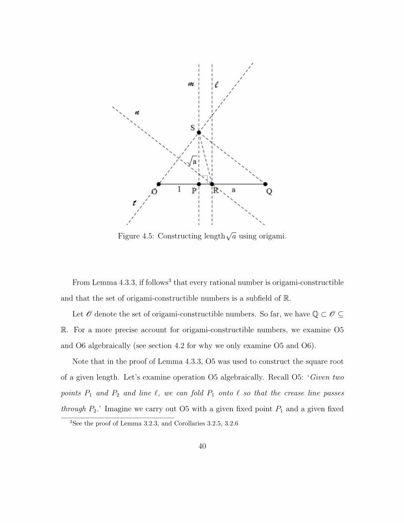
45 Constructing lengthradica using origami 40
46 Lines folding point P onto line ` 41
47 Folding point P onto a line ` 42
48 Applying O6 to P1 = (0 1) P2 = (a b) and `1 y = minus1 44
49 An example of a cubic curve 46
410 An example of a cubic curve 47
vii
411 Line f with slope m 49
412 Constructing length 3radic
2 using origami 60
413 Trisecting an angle θ using origami 61
414 Trisecting an obtuse angle using origami 62
415 A regular polygon and its central angle 62
viii
Chapter 1
Introduction
11 Geometric Constructions
There are various tools such as the straightedge and compass one can use to con-
struct geometric objects Each construction tool has its unique rules of operating
when making geometric constructions To construct a geometric object means to
carry out a set of operations the tool permits that collectively produce the geometri-
cal object Note that constructing a geometric object differs from making a freehand
illustration or drawing of the object
Take the classical straightedge and compass as an example In straightedge and
compass constructions one can use either tool but not both simultaneously The
straightedge can only be used to draw the line through two given points but cannot
be used to measure length The compass can be used to construct a circle or arc with
a given center and point on the circle or arc Some basic straightedge and compass
constructions will be discussed in Chapter 3 (see Figures 31 and32)
1
The system of assumptions or axioms concerning the unique rules of operating for
each tool have a profound effect on what objects are constructible within a particular
framework While the classical framework of straightedge and compass constructions
(described below) is better known one can expand this framework by adding other
constructions (for example see Section 34 on the marked ruler and verging) or
one can consider new frameworks such as constructions by origami which will be
explored later in detail
The straightedge and compass the rules of construction and the study of con-
structible objects go back to the ancient Greeks and Egyptians For example con-
sider the famous Greek geometry problems
Using only straightedge and compass
1 (Doubling a cube) Is it possible to construct a cube whose volume is equivalent
to twice the volume of a given cube
2 (Trisecting an angle) Is it possible to trisect any given angle of measure θ
3 (Squaring a circle) Is it possible to construct a square whose area is equivalent to
that of a given circle
The study of constructible objects including the famous Greek geometry problems
emerged from everyday life such as in architecture and surveying [14] For example
according to Cox [4 page 266] there are two versions of the origin of doubling a cube
King Minos and the tomb of his son the cubical altar of Apollo in Athens Both
involved the construction of some architectural structure Although straightedge
and compass may have lost their place in our everyday lives geometric constructions
2
with straightedge and compass are still introduced in high school geometry providing
opportunities for students to better understand definitions and characteristics of
geometric figures
Going back to the Greek geometry problems the Greeks were not able to solve
the famous geometry problems at that time but the search for solutions led to other
mathematical creations (eg Hippocrates of Chios and the lune Hippias of Elis
and the quadratrix Menaechmus and parabolas the spiral of Archimedes) [4] In
1837 Wantzel showed that trisecting an angle and doubling a cube by straightedge
and compass were not always possible in 1882 Lindemann showed that squaring
the circle was impossible with straightedge and compass when he showed that π is
transcendental over Q [4] The proofs will be discussed in Chapter 3
The development of Modern algebra and coordinate geometry played a big role in
solving these problems and studying geometric constructions with other various tools
such as the marked ruler divider Origami (paperfolding) and Mira Specifically
the collection of lengths that various geometric tools can theoretically construct
became associated with various algebraic fields Among the various tools of geometric
constructions this thesis presents an exposition of origami constructible objects and
its associated algebraic field
12 Origami Constructions
Origami is the Japanese art of paper folding in which one starts with a square-
shaped sheet of paper and folds it into various three-dimensional shapes Typically
3
in origami one starts with an unmarked square-shaped sheet of paper using only
folding (usually cutting is not allowed) with the goal of constructing reference points
that are used to define folds that produce the final object [14] Reference points
can be points on the square-shaped papers (eg the four corners) but also can be
generated as intersections of lines formed by the edges of the paper or creases that
align a combination of points edges and creases [14]
Although origami originally started as an activity in everyday life origami has
become a topic of research According to Lang [14 page 42] ldquoStarting in the 1970s
several folders began to systematically enumerate the possible combinations of folds
to study what types of distances were constructible by combining them in various
waysrdquo In the 1980s several researchers identified a fixed set of well-defined folds
one can make in origami constructions (see Figure 41) and formalized the modern
study of geometric constructions with origami
In origami theory starting with the fixed set of well-defined folds researchers
have investigated the objects possible or impossible to construct using origami For
example it was shown that trisecting an angle and doubling a cube are possible
with origami constructions however constructing the regular 11-gon or solving the
general quintic equation was shown impossible [2]
There is an international conference lsquoThe International Meeting on Origami Sci-
ence Mathematics and Educationrsquo at which the origami community have gathered
since 1989 to discuss origami in science mathematics education technology and
art [18] With the development of the computer computational systems of origami
simulation have been developed and a more systematic study of origami has evolved
4
Origami has also been applied to other fields such as science and technology Ac-
cording to Lucero [15] the application of origami can be found in aerospace and
automotive technology materials science computer science biology civil engineer-
ing robotics and acoustics However as folding techniques have been adapted in
industry more rigor and formalization of origami theory has been called for For
example Kasem et al [13] and Ghourabi et al [7] called for more precise statements
of the folding operations and introduced the extension of origami constructions with
an additional tool of the compass
13 Overview of Thesis Chapters
In Chapter 2 I will first review the basic definitions and theorems of field theory
that will be used in subsequent chapters In Chapter 3 I will discuss the more com-
monly known straightedge and compass constructions as a lead into the discussion
on origami constructions In Chapter 4 I will introduce the basic single-fold opera-
tions of origami and discuss what it means for an object to be origami-constructible
Through algebraizing geometric constructions with origami I will show how to prove
or disprove the constructibility of some objects In Chapter 5 I end this thesis with
closing remarks and some additional thoughts for future studies
5
Chapter 2
Preliminaries in Field Theory
In this Chapter 2 I will review the basic definitions and theorems of field theory
that will be used in subsequent chapters
21 Basic Definitions
Definition 211 (Group) A group G is a set together with a binary operation
(usually denoted by middot and called the group operation) that satisfy the following
(i) (a middot b) middot c = a middot (b middot c) for all a b c isin G (Associativity)
(ii) There exists an element e isin G (called the identity of G) such that amiddote = emiddota = a
for all a isin G (Identity)
(iii) For each a isin G there exists an element aminus1 isin G (called the inverse of a) such
that a middot aminus1 = aminus1 middot a = e (Inverse)
The group G is called abelian if a middot b = b middot a for all a b isin G
6
Definition 212 (Subgroup) Given a group G a subset H of G is a subgroup of
G (denoted H le G) if H is nonempty and closed under multiplication and inverse
ie a b isin H rArr ab isin H and aminus1 isin H
Whereas the theory of groups involves general properties of objects having an
algebraic structure defined by a single binary operation the theory of rings involves
objects having an algebraic structure defined by two binary operations related by
the distributive laws [5 p222]
Definition 213 (Ring) A ring R is a set together with two operations +times
(addition and multiplication) that satisfy the following
(i) R is an abelian group under addition (denote the additive identity 0 and additive
inverse of element a as minusa)
(ii) (atimes b)times c = atimes (btimes c) for all a b c isin R (Multiplicative associativity)
(iii) (a + b) times c = (a times c) + (b times c) and a times (b + c) = (a times b) + (a times c) for all
a b c isin R (Left and right distributivity)
(iv) There exists an element 1 isin R (called the multiplicative identity) such that
1times a = atimes 1 = a for all a isin R (multiplicative unit)
Rings may also satisfy optional conditions such as
(v) atimes b = btimes a for all a b isin R
In this case the ring R is called commutative
7
(vi) For every a isin R 0 there exists an element aminus1 isin R such that a times aminus1 =
1 = aminus1 times a
In this case the ring R is called a division ring
Definition 214 (Subring) Given a ring R a subset S of R is a subring of R if
S is a subgroup of R closed under multiplication and if 1 isin S In other words S is
a subring of R if the operations of addition and multiplication in R restricted to S
give S the structure of a ring
A commutative division ring (a ring that satisfies all conditions (i) through (vi)
in Definition 213) is called a field More concisely
Definition 215 (Field) A field is a set F together with two binary operations +
and middot that satisfy the following
(i) F is an abelian group under + (with identity 0)
(ii) Ftimes = F minus 0 is an abelian group under middot (with identity 1)
(iii) a middot (b+ c) = (a middot b) + (a middot c) for all a b c isin F (Distributivity)
For example any set closed under all the arithmetic operations +minustimesdivide (divi-
sion by nonzero elements) is a field
22 Field Theory
Of particular interest in this thesis is the idea of extending a given field into a
(minimally) larger field so that the new field contains specific elements in addition
to all the elements of the given field We first define a field extension
8
Definition 221 If K is a field with subfield F then K is an extension field of
F denoted KF (read ldquoK over F rdquo) If KF is a field extension then K is a vector
space over F with degree dimFK denoted [K F ] The extension is finite if [K F ]
is finite and infinite otherwise
Definition 222 If K is an extension of field F and if α β middot middot middot isin K then the
smallest subfield of K containing F and α β middot middot middot isin K is called the field generated
by α β middot middot middot over F denoted F (α β middot middot middot ) An extension KF is finitely generated
if there are finitely many elements α1 αk isin K such that K = F (α1 αk) If
the field is generated by a single element α over F then K is a simple extension
of F with α a primitive element for the extension K = F (α)
We are specifically interested in field extensions that contain roots of specific
polynomials over a given field with the new field extending the field The following
propositions of such field extensions are taken as given without proof1
Proposition 223 Given any field F and irreducible polynomial p(x) isin F [x] there
exists an extension of F in which p(x) has a root Namely the field K = F [x](p(x))
in which F [x](p(x)) is the quotient of the ring F [x] by the maximal ideal (p(x))
Further if deg(p(x)) = n and α isin K denotes the class of x modulo p(x) then
1 α α2 αnminus1 is a basis for K as a vector space over F with [K F ] = n so
K = a0 + a1α + middot middot middot+ anminus1αnminus1|a0 anminus1 isin F
1For a detailed proof of these statements see Dummit amp Foote [5 pp 512-514]
9
While Proposition 223 states the existence of an extension field K of F that
contains a solution to a specific equation the next proposition indicates that any
extension of F that contains a solution to that equation has a subfield isomorphic to
K and that K is the smallest extension of F (up to isomorphism) that contains such
a solution
Proposition 224 Given any field F and irreducible polynomial p(x) isin F [x] sup-
pose L is an extension field of F containing a root α of p(x) and let F (α) denote the
subfield of L generated over F by α Then F (α) sim= F [x](p(x)) If deg(p(x)) = n
then F (α) = a0 + a1α + a2α2 + middot middot middot+ anminus1α
nminus1|a0 a1 anminus1 isin F sube L
Example 225 Consider F = R and p(x) = x2 + 1 an irreducible polynomial over
R Then we obtain the field K = R(x2 +1) sim= R(i) sim= R(minusi) an extension of R that
contains the solution of x2 + 1 = 0 [K F ] = 2 with K = a+ bi|a b isin R = C
The elements of a field extension K of F need not always be a root of a polynomial
over F
Definition 226 Let K be an extension of a field F The element α isin K is alge-
braic over F if α is a root of some nonzero polynomial f(x) isin F [x] If α isin K is
not the root of any nonzero polynomial over F then α is transcendental over F
The extension KF is algebraic if every element of K is algebraic over F
Proposition 227 Let K be an extension of a field F and α algebraic over F Then
there is a unique monic irreducible polynomial mα(x) isin F [x] with α as a root This
polynomial mα(x) is called the minimal polynomial for α over F and deg(mα) is
the degree of α So F (α) sim= F [x](mα(x)) with [F (α) F ] = deg(mα(x)) = degα
10
Proposition 228 If α is algebraic over F ie if α is a root to some polynomial
of degree n over F then [F (α) F ] le n On the other hand if [F (α) F ] = n
then α is a root of a polynomial of degree at most n over F It follows that any finite
extension KF is algebraic
Example 229 (Quadratic Extensions over F with char(F ) 6= 2) Let K an ex-
tension of a field F with the char(F ) 6= 22 and [K F ] = 2 Let α isin K but
α isin F Then α must be algebraic ie a root of a nonzero polynomial over F of
degree at most 2 by Proposition 228 Since α isin F this polynomial cannot be
of degree 1 Hence by Proposition 227 the minimal polynomial of α is a monic
quadratic mα(x) = x2 + bx + c with b c isin Q F sub F (α) sube K and [K F ] = 2 so
K = F (α) (see Proposition 227 and 228) From the quadratic formula (possible
since char(F ) 6= 2) the elements
minusbplusmnradicb2 minus 4c
2isin F (
radicd)
are roots of mα(x) with d = b2 minus 4c We can by Proposition 227 identify F (α)
with a subfield of F (radicd) by identifying α with 1
2(minusbplusmn
radicd) (either sign choice works)
We know that d is not a square in F since α isin F By construction F (α) sub F (radicd)
On the other handradicd = ∓(b + 2α) isin F (α) so F (
radicd) sube F (α) Therefore F (α) =
F (radicd) As such any extension K of F of degree 2 is of the form F (
radicd) where
d isin F is not a square in F Conversely any extension of the form F (radicd) where
2The characteristic of a field F is the smallest integer n such that n middot 1F = 0 If such n does notexist then the characteristic is defined to be 0
11
d isin F is not a square in F is an extension of degree 2 over F Such an extension is
called a quadratic extension over F
Particularly when F = Q any extension K of Q of degree 2 is of the form Q(radicd)
where 0 lt d isin Q is not a square in Q Conversely any extension of the form Q(radicd)
where 0 lt d isin Q is not a square in Q is an extension of degree 2 over Q Such an
extension is called a quadratic extension over Q
Theorem 2210 (Tower Rule) Let F a field extension of E and K a field extension
of F Then K is a field extension of E of degree [K E] = [K F ][F E]
Proof Suppose [F E] = m and [K F ] = n are finite Let α1 αm a basis for F
over E and β1 βn a basis for K over F Let β any element of K Since β1 βn
are a basis for K over F there are elements b1 bn isin F such that
β = b1β1 + b2β2 + middot middot middot+ bnβn (21)
Since α1 αm are a basis for F over E there are elements ai1 ain isin E i =
1 2 m such that each
bi = ai1α1 + ai2α2 + middot middot middot+ ainαn (22)
Substituting (22) into (22) we obtain
β =nsumj=1
msumi=1
aij(αiβj) aij isin F (23)
12
In other words any element of K can be written as a linear combination of the nm
elements αiβj with coefficients in F Hence the vectors αiβj span K as a vector space
over E
Suppose β = 0 in (23)
β =nsumj=1
msumi=1
aij(αiβj) =nsumj=1
(msumi=1
aijαi
)βj
Since β1 βn are linearly independentsumm
i=1 aijαi = 0 for all j = 1 n Since
α1 αm are linearly independent aij = 0 for all i = 1 2 m and j = 1 n
Therefore the nm elements αiβj are linearly independent over E and form a basis
for K over E Therefore [K E] = nm = [K F ][F E] If either [K F ] or [F E]
is infinite then there are infinitely many elements of K or F respectively so [K E]
is also infinite On the other hand if [K E] is infinite then at least one of [K F ]
and [F E] has to be infinite since if they are both finite the above proof shows that
[K E] is finite
13
Chapter 3
Straightedge and Compass
Constructions
To investigate the constructability of geometric objects using straightedge and com-
pass such as the problems posed by the Greeks we translate geometric construc-
tions into algebraic terms In this chapter we explore geometric constructions with
straightedge and compass and constructible numbers
31 Initial Givens Operations and Basic Construc-
tions
In straightedge and compass constructions two points say O and P are initially
given Starting with these given points we can carry out the following operations
with straightedge and compass which produce lines and circles
Operations of straightedge and compass constructions
Given two constructed points we can
14
C1 construct the line connecting the two points or
C2 construct a circle centered at one point and passing through the other point
We can also construct the intersection of constructed lines or circles which gives new
points
P1 We can construct the point of intersection of two distinct lines
P2 We can construct points of intersection of a line and a circle
P3 We can construct points of intersection of two distinct circles
Repeating C1 C2 with P1 P2 P3 on OP produces more constructible points
A constructible point is any point one can construct in a finite number of steps of
combinations of C1 C2 P1 P2 or P3
Examples of basic straightedge and compass constructions
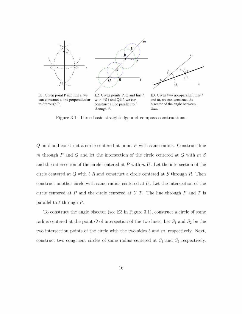
Recall the following basic constructions in Figure 31 from high school geometry
For example to construct the perpendicular line through point P (see E1 in Fig-
ure 31) construct a circle of some radius centered at point P and let Q1 and Q2
be the two intersection points of the circle with ` Next construct circles centered
at Q1 and Q2 respectively whose radius is the distance between Q1 and Q21 These
two circles will intersect in two new points R1 and R2 The line through R1 and R2
passes through P and is perpendicular to `
Given points PQ and line ` with P isin ` and Q isin l to construct a line parallel
to ` through P (see E2 in Figure 31) construct a circle of some radius centered at
1The radius can be any length greater than half the distance between Q1 and Q2 to allow thetwo circles to intersect
15
Figure 31 Three basic straightedge and compass constructions
Q on ` and construct a circle centered at point P with same radius Construct line
m through P and Q and let the intersection of the circle centered at Q with m S
and the intersection of the circle centered at P with m U Let the intersection of the
circle centered at Q with ` R and construct a circle centered at S through R Then
construct another circle with same radius centered at U Let the intersection of the
circle centered at P and the circle centered at U T The line through P and T is
parallel to ` through P
To construct the angle bisector (see E3 in Figure 31) construct a circle of some
radius centered at the point O of intersection of the two lines Let S1 and S2 be the
two intersection points of the circle with the two sides ` and m respectively Next
construct two congruent circles of some radius centered at S1 and S2 respectively
16
Let point T one of the two intersections of the two circles The line through O and
T bisects the angle between lines ` and m These examples will be useful later
32 Constructible Numbers
Now we translate geometric distances obtained through constructions into algebraic
terms by associating lengths with elements of the real numbers Given a fixed unit
distance 1 we determine any distance by its length 1r = r1 isin R
Definition 321 A real number r is constructible if one can construct in a
finite number of steps two points which are a distance of |r| apart
The set of real numbers that are associated with lengths in R obtained by straight-
edge and compass constructions together with their negatives are constructible el-
ements of R Henceforth we do not distinguish between constructible lengths and
constructible real numbers
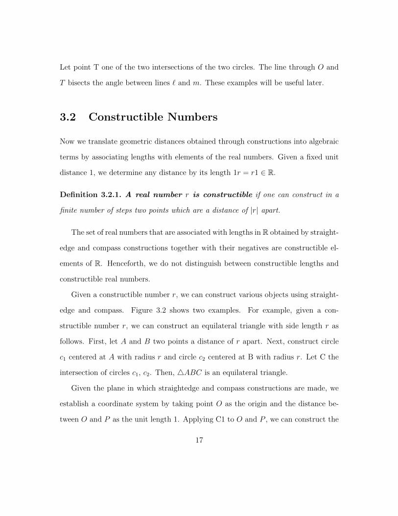
Given a constructible number r we can construct various objects using straight-
edge and compass Figure 32 shows two examples For example given a con-
structible number r we can construct an equilateral triangle with side length r as
follows First let A and B two points a distance of r apart Next construct circle
c1 centered at A with radius r and circle c2 centered at B with radius r Let C the
intersection of circles c1 c2 Then 4ABC is an equilateral triangle
Given the plane in which straightedge and compass constructions are made we
establish a coordinate system by taking point O as the origin and the distance be-
tween O and P as the unit length 1 Applying C1 to O and P we can construct the
17
Figure 32 Two straightedge and compass constructions starting with given lengthr
x-axis Applying E1 to the x-axis and point O we can construct the y-axis Then
the coordinates of the two given points O and P are (0 0) and (1 0) respectively
on the Cartesian plane As such using our points O and P we can construct a
coordinate system in the plane and use this to represent our points as ordered pairs
ie elements of R22 We then have
Lemma 322 A point (a b) isin R2 is constructible if and only if its coordinates
a and b are constructible elements of R
Proof We can construct distances along lines (see E4 in Figure 32) that are perpen-
dicular and we can make perpendicular projections to lines (apply E1) Then the
point (a b) can be constructed as the intersection of such perpendicular lines On
2The plane can be taken as the field of complex numbers C with the x-axis representing thereal numbers and the y-axis representing the imaginary numbers
18
the other hand if (a b) is constructible then we can project the constructed point to
the x-axis and y-axis (apply E1) and thus the coordinates a and b are constructible
as the intersection of two constructible lines
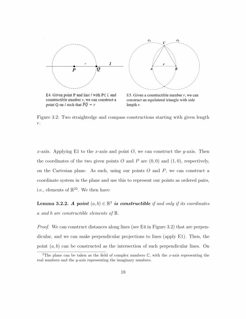
Lemma 323 Every n isin Z is constructible
Proof Construct the unit circle centered at P Then by P2 the intersection of
that unit circle and the x-axis 2 is constructible Next construct the unit circle
centered at 2 Then by P2 the intersection of that unit circle and the x-axis 3 is
constructible Iterating this process of constructing the intersection of the unit circle
and the x-axis (see Figure 33) shows that every n isin Z is constructible
Figure 33 The construction of n isin Z
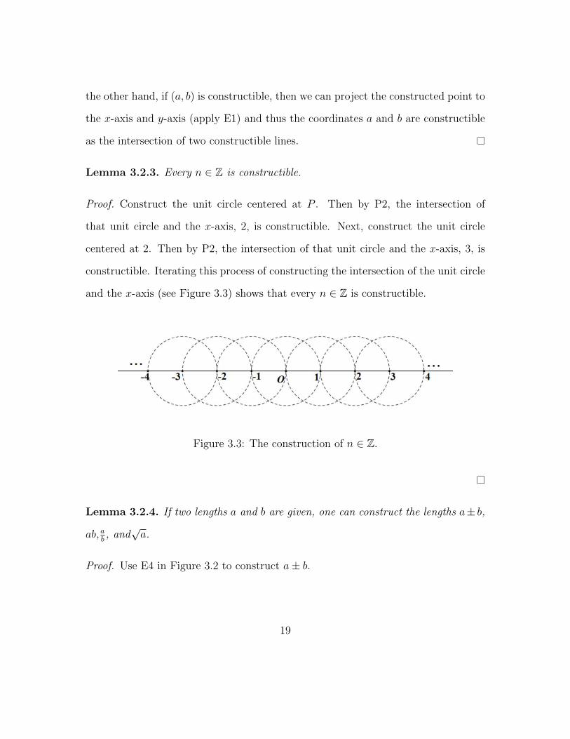
Lemma 324 If two lengths a and b are given one can construct the lengths aplusmn b
abab and
radica
Proof Use E4 in Figure 32 to construct aplusmn b
19
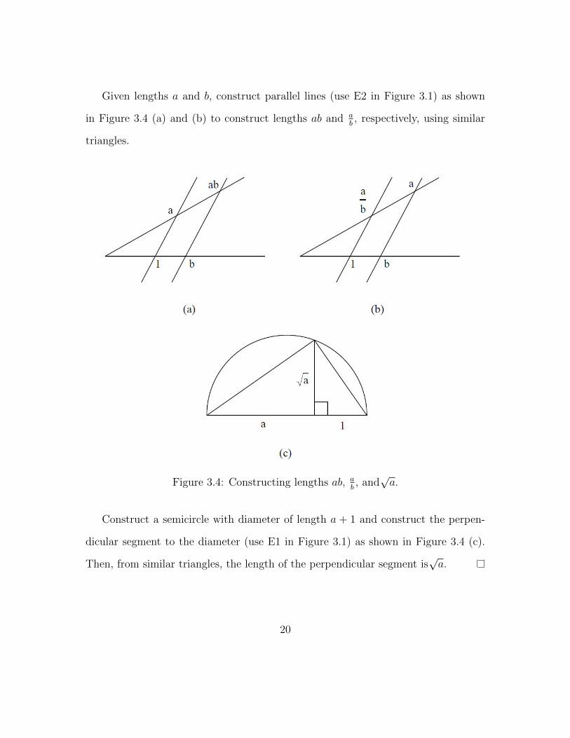
Given lengths a and b construct parallel lines (use E2 in Figure 31) as shown
in Figure 34 (a) and (b) to construct lengths ab and ab respectively using similar
triangles
Figure 34 Constructing lengths ab ab and
radica
Construct a semicircle with diameter of length a + 1 and construct the perpen-
dicular segment to the diameter (use E1 in Figure 31) as shown in Figure 34 (c)
Then from similar triangles the length of the perpendicular segment isradica
20
Lemma 34 implies that straightedge and compass constructions are closed un-
der addition subtraction multiplication division and taking square roots The
following two corollaries are immediate results
Corollary 325 The set of constructible numbers is a a subfield of R
Proof From Lemma 324 straightedge and compass constructions are closed under
addition subtraction multiplication and division (by nonzero elements) in R so the
set of constructible numbers is a subfield of R
Corollary 326 Every rational number is constructible
Proof From Lemma 323 every integer is constructible From Lemma 324 every
quotient of a pair of integers is constructible So all rationals are constructible
From Corollary 326 we can construct all points (a b) isin R2 whose coordinates
are rational We can also construct additional real numbers by taking square roots
(from Lemma 324) so the the set of constructible numbers form a field strictly
larger than Q Let C denote the set of constructible numbers with straightedge and
compass So far we proved Q sub C sube R In order to determine precisely what C
consists of we create algebraic equations for points lines and circles
First we examine the equations of constructible lines and circles
Lemma 327 Let F be an arbitrary subfield of R
(1) A line that contains two points whose coordinates are in F has an equation of
the form ax+ by + c = 0 where a b c isin F
21
(2) A circle with center whose coordinates are in F and radius whose square is in F
has an equation of the form x2 + y2 + rx+ sy + t = 0 where r s t isin F
Proof (1) Suppose (x1 y1) (x2 y2) are two points on the line such that x1 x2 y1 y2 isin
F If x1 = x2 then the equation of the line is x minus x1 = 0 If x1 6= x2 then the
equation of the line is
y minus y1 =y1 minus y2x1 minus x2
(xminus x1)
Rearranging both sides we obtain
(y1 minus y2x1 minus x2
)xminus y minus (y1 minus y2x1 minus x2
)x1 + y1 = 0
Since F is a field and x1 x2 y1 y2 isin F each coefficient is an element of F
(2) Suppose (x1 y1) is the center and k the radius such that x1 x2 k isin F Then the
equation of the circle is
(xminus x1)2 + (y minus y1)2 = k2
Rearranging the equation we obtain
x2 + y2 minus 2x1xminus 2y1y + x12 + y1
2 + k2 = 0
Since F is a field and x1 x2 k isin F each coefficient is an element of F
22
Recall that from P1 P2 P3 we can determine constructible points as intersec-
tions of two lines a line and a circle or of two circles
Lemma 328 Let F be an arbitrary subfield of R Let l1 l2 two constructible lines
and c1 c2 two constructible circles Then
(1) if l1 l2 intersect the coordinates of the point of intersection are elements of F
(2) if l1 c1 intersect the coordinates of the points of intersection are elements of F
or some quadratic extension field F (radicd)
(3) and if c1 c2 intersect the coordinates of the points of intersection are elements
of F or some quadratic extension field F (radicd)
Proof (1) Let l1 l2 each have equations
l1 a1x+ b1y + c1 = 0
l2 a2x+ b2y + c2 = 0
where ai bi ci isin F Solving these linear equations simultaneously gives solutions
also in F Therefore the coordinates of the point of intersection of l1 l2 are
elements of F
(2) Let l1 c1 each have equations
l1 a1x+ b1y + c1 = 0
c1 x2 + y2 + r1x+ s1y + t1 = 0
23
where a1 b1 c1 r1 s1 t1 isin F Solving these equations simultaneously gives a
quadratic equation with coefficients all in F Hence the solutions will lie in
a field of the form F (radicd) where d isin F (see Example 229) Therefore the
coordinates of the points of intersection of l1 c1 are elements of F (radicd)
(3) Let c1 c2 each have equations
c1 x2 + y2 + r1x+ s1y + t1 = 0
c2 x2 + y2 + r2x+ s2y + t2 = 0
where ri si ti isin F Subtracting the equation of c2 from c1 gives us a linear
equation
(r1 minus r2)x+ (s1 minus s2)y + (t1 minus t2) = 0
Solving this linear equation simultaneously with the equation of c1 gives a quadratic
equation with coefficients all in F Hence the solutions will lie in a field of the
form F (radicd) where d isin F Therefore the coordinates of the points of intersection
of c1 c2 are elements of F (radicd)
Theorem 329 Let r isin R Then r isin C if and only if there is a finite sequence
of fields Q = F0 sub F1 sub F2 sub middot middot middot sub Fn sub R such that r isin Fn and for each
i = 0 1 n [Fi Fiminus1] = 2
Proof (rArr) Suppose r isin C As discussed in section 31 r isin C only when it could
be constructed through operations C1 C2 C3 with straightedge and compass and
24
their intersections P1 P2 P3 From Lemma 328 such straightedge and compass
constructions in F involve a field extension of degree one or two From induction on
the number of constructions required to construct r there must be a finite sequence
of fields Q = F0 sub F1 sub middot middot middot sub Fn sub R such that r isin Fn with [Fi Fiminus1] = 2
(lArr) Suppose Q = F0 sub F1 sub F2 sub middot middot middot sub Fn sub R such that [Fi Fiminus1] = 2
Then Fi = Fiminus1[radicdi] for some di isin Fi (see Example 229) If n = 0 then r isin F0 = Q
and Q sub C from Corollary 326 Suppose any element of Fn is constructible for
when n = kminus 1 Then any dk isin Fkminus1 is constructible which implies thatradicdk is also
constructible from Lemma 324 Therefore any element of Fk = Fkminus1[radicdk] is also
constructible From mathematical induction any r isin Fn is constructible
Since straightedge and compass constructions involve a field extension of Q with
degree at most 2 the operations can produce elements of at most a quadratic ex-
tension of Q So C is the smallest field extension of Q that is closed under taking
square roots
Corollary 3210 If r isin C then [Q(r) Q] = 2k for some integer k ge 0
Proof From Theorem 329 if r isin C there is a finite sequence of fields Q = F0 sub
middot middot middot sub Fn sub R such that r isin Fn and for each i = 0 1 n [Fi Fiminus1] = 2 So by
the Tower Rule (Theorem 2210)
[Fn Q] = [Fn Fnminus1] middot middot middot [F1 F0] = 2n
Since Q sub Q(r) sub Fn again by the Tower Rule [Q(r) Q]|[Fn Q] = 2n so if r isin C
then [Q(r) Q] = 2k for some integer k ge 0
25
It follows that every constructible number is algebraic over Q and the degree of
its minimal polynomial over Q is a power of 2
33 Impossibilities
Now we can revisit the three classic Greek geometry problems
Theorem 331 [Doubling the cube] It is impossible to construct an edge of a cube
with volume 2 using straightedge and compass
Proof An edge of such a cube would have length 3radic
2 a root of p(x) = x3 minus 2 By
the rational root test p(x) is irreducible so it is the minimal polynomial for 3radic
2 over
Q From Proposition 227 [Q( 3radic
2) Q] = 3 which is not a power of 2 So by
Corollary 3210 3radic
2 is not constructible
Before we prove the impossibility of trisecting an angle we first define a con-
structible angle and prove the following Lemma
Definition 332 An angle θ is constructible if one can construct two lines ` and
m with angle θ between them
Lemma 333 An angle θ is constructible if and only if cos θ and sin θ are both
constructible numbers
Proof (rArr) Using E1 we can construct a line ` perpendicular to the x-axis through
point P on angle θ at distance 1 from the origin Hence the intersection of ` and
the x-axis cos θ is constructible Similarly using E1 we can construct sin θ
26
(lArr) From Definition 321 since cos θ and sin θ are both constructible the point
(cos θ sin θ) is constructible Hence angle θ is constructible
Theorem 334 [Trisecting an angle] Not all angles can be trisected using only
straightedge and compass
Proof We show that it is impossible to trisect a 60 angle Note that 60 is con-
structible as the angle between two sides of an equilateral triangle (see construction
E5 in Figure 32) From Lemma 333 it suffices to show that cos 20 is not con-
structible
From the triple angle formulas of trigonometry we know
cos 3α = cos3 αminus 3 cosα sin2 α = 4 cos3 αminus 3 cosα
Substituting α = 20 12
= 4 cos3 20 minus 3 cos 20 Thus cos 20 is a root of the
polynomial p(x) = 8x3 minus 6x minus 1 But p(x) is irreducible in Q by the rational root
test So by Proposition 227 [Q(cos 20) Q] = 3 which is not a power of 2
Therefore cos 20 is not constructible by Corollary 3210
Proposition 335 [Squaring the circle] It is impossible to construct an edge of a
square with same area as the unit circle using straightedge and compass
Because the proof is beyond the scope of this thesis the last Greek problem is
presented as a proposition Proposition 335 is based on the fact that [Q(π) Q] is
not finite and hence π is not constructible shown by Lindemann in 1882 [4]
27
34 Marked Rulers and Verging
One can add to the straightedge and compass axioms by allowing a new operation
involving a straightedge marked with a distance ie a marked ruler A marked
ruler is a straightedge with two marks on its edge that can be used to mark off unit
distances along a line The new operation is called verging [16] and with it one can
make geometric constructions that were not possible with the standard straightedge
and compass as previously described Below we explore the verging operation and
one example of a marked ruler and compass construction which was not possible
with the standard straightedge and compass
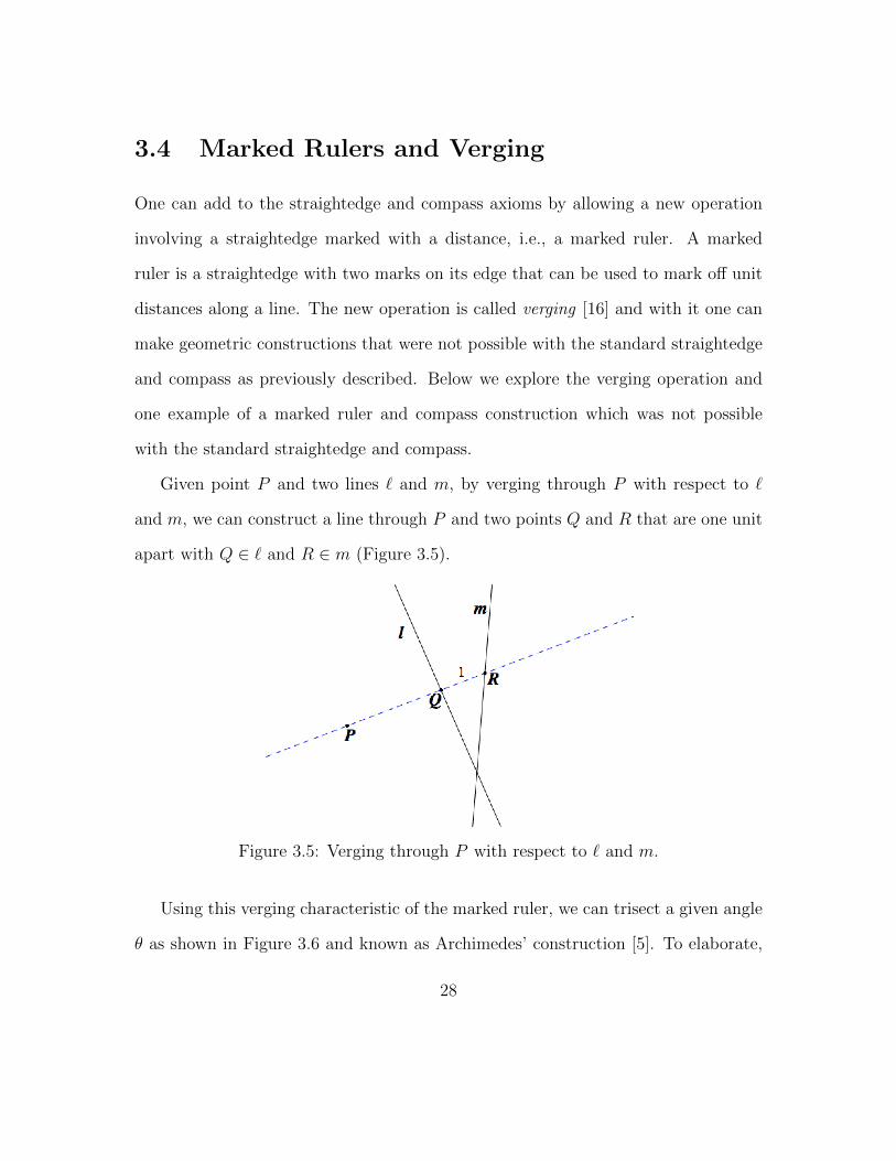
Given point P and two lines ` and m by verging through P with respect to `
and m we can construct a line through P and two points Q and R that are one unit
apart with Q isin ` and R isin m (Figure 35)
Figure 35 Verging through P with respect to ` and m
Using this verging characteristic of the marked ruler we can trisect a given angle
θ as shown in Figure 36 and known as Archimedesrsquo construction [5] To elaborate
28
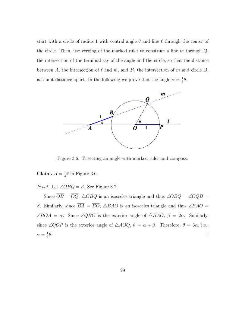
start with a circle of radius 1 with central angle θ and line ` through the center of
the circle Then use verging of the marked ruler to construct a line m through Q
the intersection of the terminal ray of the angle and the circle so that the distance
between A the intersection of ` and m and B the intersection of m and circle O
is a unit distance apart In the following we prove that the angle α = 13θ
Figure 36 Trisecting an angle with marked ruler and compass
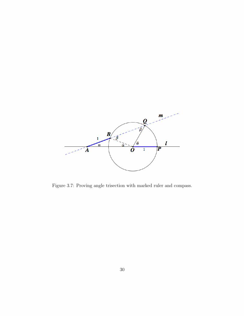
Claim α = 13θ in Figure 36
Proof Let angOBQ = β See Figure 37
Since OB = OQ 4OBQ is an isosceles triangle and thus angOBQ = angOQB =
β Similarly since BA = BO 4BAO is an isosceles triangle and thus angBAO =
angBOA = α Since angQBO is the exterior angle of 4BAO β = 2α Similarly
since angQOP is the exterior angle of 4AOQ θ = α + β Therefore θ = 3α ie
α = 13θ
29
Figure 37 Proving angle trisection with marked ruler and compass
30
Chapter 4
Origami Constructions
In this chapter we investigate the constructibility of geometric objects using origami
Similar to the discussion in Chapter 3 we translate geometric constructions into al-
gebraic terms and explore origami constructions and origami-constructible numbers
41 Initial Givens and Single-fold Operations
In origami constructions we consider the plane on which origami occurs as a sheet of
paper infinitely large on which two points say O and P are initially given Origami
constructions consist of a sequence of single-fold operations that align combinations
of points and lines in the plane A single-fold refers to folding the paper once a new
fold can only be made after the paper is unfolded Each single-fold leaves a crease
which acts as a origami-constructed line Intersections among origami-constructed
lines define origami-constructed points
31
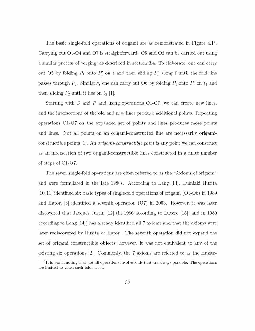
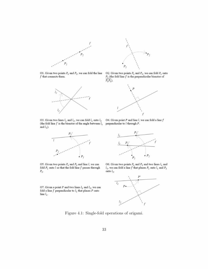
The basic single-fold operations of origami are as demonstrated in Figure 411
Carrying out O1-O4 and O7 is straightforward O5 and O6 can be carried out using
a similar process of verging as described in section 34 To elaborate one can carry
out O5 by folding P1 onto P prime1 on ` and then sliding P prime1 along ` until the fold line
passes through P2 Similarly one can carry out O6 by folding P1 onto P prime1 on `1 and
then sliding P2 until it lies on `2 [1]
Starting with O and P and using operations O1-O7 we can create new lines
and the intersections of the old and new lines produce additional points Repeating
operations O1-O7 on the expanded set of points and lines produces more points
and lines Not all points on an origami-constructed line are necessarily origami-
constructible points [1] An origami-constructible point is any point we can construct
as an intersection of two origami-constructible lines constructed in a finite number
of steps of O1-O7
The seven single-fold operations are often referred to as the ldquoAxioms of origamirdquo
and were formulated in the late 1980s According to Lang [14] Humiaki Huzita
[1011] identified six basic types of single-fold operations of origami (O1-O6) in 1989
and Hatori [8] identified a seventh operation (O7) in 2003 However it was later
discovered that Jacques Justin [12] (in 1986 according to Lucero [15] and in 1989
according to Lang [14]) has already identified all 7 axioms and that the axioms were
later rediscovered by Huzita or Hatori The seventh operation did not expand the
set of origami constructible objects however it was not equivalent to any of the
existing six operations [2] Commonly the 7 axioms are referred to as the Huzita-
1It is worth noting that not all operations involve folds that are always possible The operationsare limited to when such folds exist
32
Figure 41 Single-fold operations of origami
33
Hatori Axioms or the Huzita-Justin Axioms These axioms are not independent it
has been shown that O1-O5 can be done using only O6 ( [2] [7])
Using exhaustive enumeration on all possible alignments of lines and points
Alperin and Lang [2] have shown that the 7 axioms are complete meaning that
the 7 operations include all possible combinations of alignments of lines and points
in Origami In other words there are no other single-fold axioms other than the
seven However Alperin and Lang [2] restricted the cases to those with a finite
number of solutions in a finite-sized paper to exclude alignments that require infinite
paper to verify They also excluded redundant alignments that do not produce new
lines or points
More recently there have been critiques of these axioms For example Kasem
et al [13] showed the impossibility of some folds discussed the cases where in-
finitely many fold lines occur and pointed out superfluous conditions in the axioms
Ghourabi et al [7 page 146] conducted a systematic algebraic analysis of the 7 ax-
ioms and claimed ldquo[w]hile these statements [the 7 axioms] are suitable for practicing
origami by hand a machine needs stricter guidance An algorithmic approach to
folding requires formal definition of fold operationsrdquo
In this thesis I assume the traditional set of 7 single-fold operations as listed
in Figure 41 and explore the origami constructions and origami numbers derived
from them In the next chapter I will discuss some of the more recent studies and
extensions of the origami axioms
34
42 Origami Constructions
421 Origami constructions in relation to straightedge and
compass constructions
In their 1995 paper Auckly and Cleveland [3] showed that the set of origami construc-
tions using only operations O1-O4 is less powerful than constructions with straight-
edge and compass In his 1998 book on geometric constructions Martin [16] showed
that a paper folding operation which he termed the ldquofundamental folding opera-
tionrdquo accounts for all possible cases of incidences between two given distinct points
and two given lines This fundamental folding operation is equivalent to O6 (re-
stricted to p1 6= p2) [2] Further Martin proved that this operation is sufficient for
the construction of all objects constructible by O1-O6 altogether including straight-
edge and compass constructions In his publication in 2000 Alperin [1] showed that
operations O2 O3 and O5 together are equivalent to axioms O1-O5 and that the
set of constructible numbers obtained by these sets of operations is exactly the set
of constructible numbers obtained by straightedge and compass
422 Some examples of basic origami constructions
Recall the Examples of Basic Constructions (31) with straightedge and compass in
Chapter 3 These constructions can be made with origami as well For example E1
and E3 are equivalent to O4 and O3 respectively E2 (constructing a line parallel to
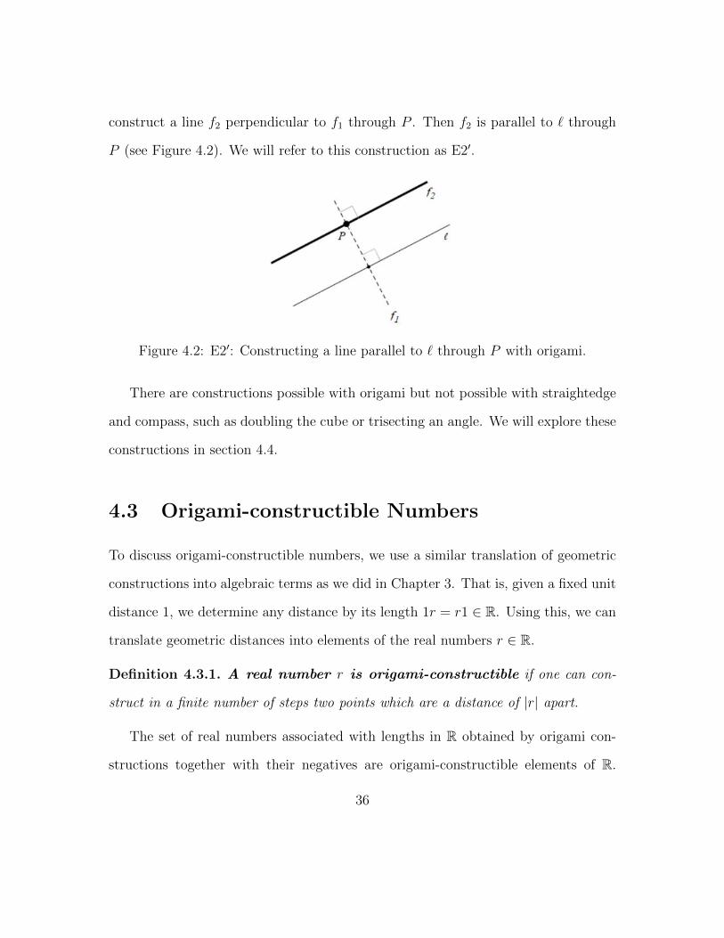
a given line ` through point P ) can be done through origami as the following Apply
O4 to construct a line f1 perpendicular to ` through P Then apply O4 again to
35
construct a line f2 perpendicular to f1 through P Then f2 is parallel to ` through
P (see Figure 42) We will refer to this construction as E2prime
Figure 42 E2prime Constructing a line parallel to ` through P with origami
There are constructions possible with origami but not possible with straightedge
and compass such as doubling the cube or trisecting an angle We will explore these
constructions in section 44
43 Origami-constructible Numbers
To discuss origami-constructible numbers we use a similar translation of geometric
constructions into algebraic terms as we did in Chapter 3 That is given a fixed unit
distance 1 we determine any distance by its length 1r = r1 isin R Using this we can
translate geometric distances into elements of the real numbers r isin R
Definition 431 A real number r is origami-constructible if one can con-
struct in a finite number of steps two points which are a distance of |r| apart
The set of real numbers associated with lengths in R obtained by origami con-
structions together with their negatives are origami-constructible elements of R
36
Henceforth we do not distinguish between origami-constructible lengths and origami-
constructible real numbers
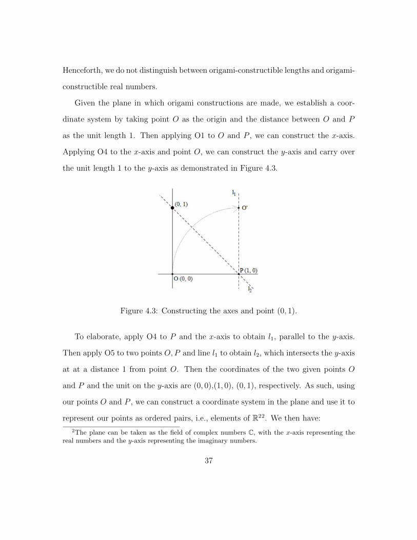
Given the plane in which origami constructions are made we establish a coor-
dinate system by taking point O as the origin and the distance between O and P
as the unit length 1 Then applying O1 to O and P we can construct the x-axis
Applying O4 to the x-axis and point O we can construct the y-axis and carry over
the unit length 1 to the y-axis as demonstrated in Figure 43
Figure 43 Constructing the axes and point (0 1)
To elaborate apply O4 to P and the x-axis to obtain l1 parallel to the y-axis
Then apply O5 to two points OP and line l1 to obtain l2 which intersects the y-axis
at at a distance 1 from point O Then the coordinates of the two given points O
and P and the unit on the y-axis are (0 0)(1 0) (0 1) respectively As such using
our points O and P we can construct a coordinate system in the plane and use it to
represent our points as ordered pairs ie elements of R22 We then have
2The plane can be taken as the field of complex numbers C with the x-axis representing thereal numbers and the y-axis representing the imaginary numbers
37
Lemma 432 A point (a b) isin R2 is origami-constructible if and only if its
coordinates a and b are origami-constructible elements of R
Proof We can origami-construct distances along perpendicular lines (apply E2rsquo in
Figure 42) and we can make perpendicular projections to lines (apply O4) Then
the point (a b) can be origami-constructed as the intersection of such perpendicular
lines On the other hand if (a b) is origami-constructible then we can project the
constructed point to the x-axis and y-axis (apply O4) and thus the coordinates a and
b are origami-constructible as the intersection of two origami-constructed lines
Since it has been shown that all straightedge and compass constructions can be
made with origami it follows that Lemmas 323 324 and Corollaries 325 326
hold in origami as well In the following Lemma we prove the closure of origami
numbers under addition subtraction multiplication division and taking square
roots by showing how to construct such lengths with origami
Lemma 433 If two lengths a and b are given one can construct the lengths aplusmn b
abab and
radica in origami
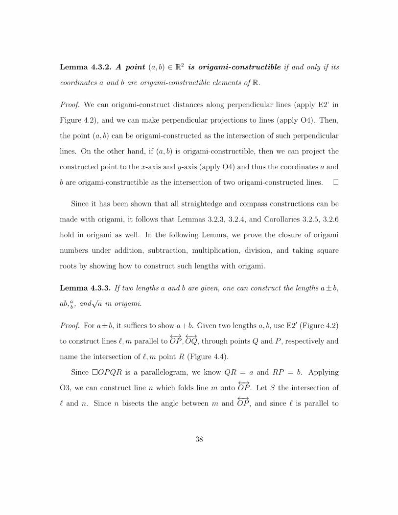
Proof For aplusmnb it suffices to show a+b Given two lengths a b use E2prime (Figure 42)
to construct lines `m parallel tolarrrarrOPlarrrarrOQ through points Q and P respectively and
name the intersection of `m point R (Figure 44)
Since OPQR is a parallelogram we know QR = a and RP = b Applying
O3 we can construct line n which folds line m ontolarrrarrOP Let S the intersection of
` and n Since n bisects the angle between m andlarrrarrOP and since ` is parallel to
38
Figure 44 Constructing length a+ b using origami
larrrarrOP we know that 4RPS is an isosceles triangle and thus PQ = b Hence we have
constructed a line segment QS with length a+ b
Given lengths a and b construct parallel lines (E2prime) as shown in Figure 34 (a)
and (b) to construct lengths ab and ab respectively using similar triangles
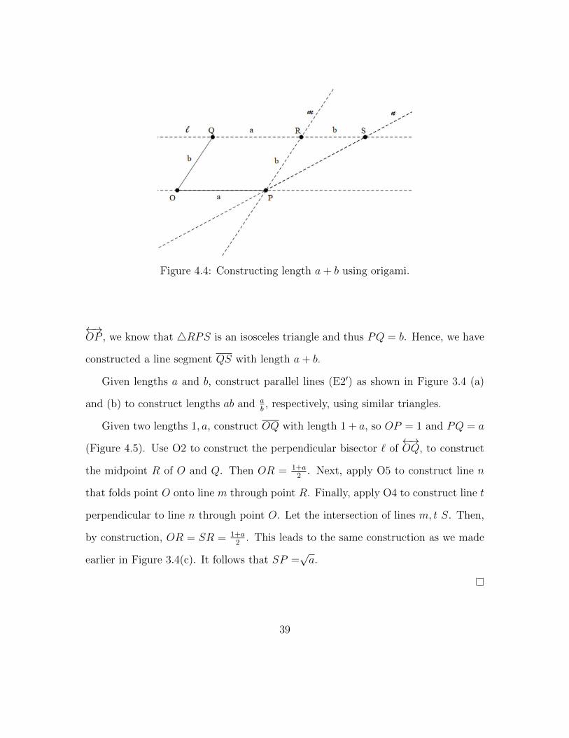
Given two lengths 1 a construct OQ with length 1 + a so OP = 1 and PQ = a
(Figure 45) Use O2 to construct the perpendicular bisector ` oflarrrarrOQ to construct
the midpoint R of O and Q Then OR = 1+a2
Next apply O5 to construct line n
that folds point O onto line m through point R Finally apply O4 to construct line t
perpendicular to line n through point O Let the intersection of lines m t S Then
by construction OR = SR = 1+a2
This leads to the same construction as we made
earlier in Figure 34(c) It follows that SP =radica
39
Figure 45 Constructing lengthradica using origami
From Lemma 433 if follows3 that every rational number is origami-constructible
and that the set of origami-constructible numbers is a subfield of R
Let O denote the set of origami-constructible numbers So far we have Q sub O sube
R For a more precise account for origami-constructible numbers we examine O5
and O6 algebraically (see section 42 for why we only examine O5 and O6)
Note that in the proof of Lemma 433 O5 was used to construct the square root
of a given length Letrsquos examine operation O5 algebraically Recall O5 lsquoGiven two
points P1 and P2 and line ` we can fold P1 onto ` so that the crease line passes
through P2rsquo Imagine we carry out O5 with a given fixed point P1 and a given fixed
3See the proof of Lemma 323 and Corollaries 325 326
40
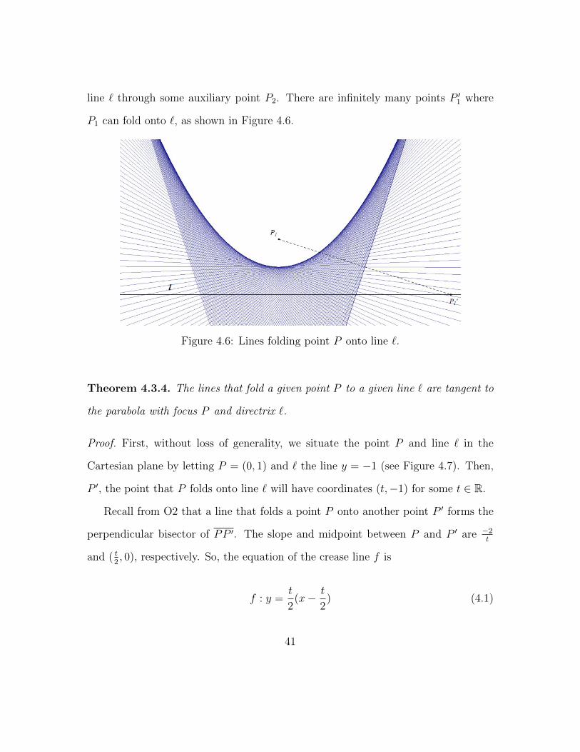
line ` through some auxiliary point P2 There are infinitely many points P prime1 where
P1 can fold onto ` as shown in Figure 46
Figure 46 Lines folding point P onto line `
Theorem 434 The lines that fold a given point P to a given line ` are tangent to
the parabola with focus P and directrix `
Proof First without loss of generality we situate the point P and line ` in the
Cartesian plane by letting P = (0 1) and ` the line y = minus1 (see Figure 47) Then
P prime the point that P folds onto line ` will have coordinates (tminus1) for some t isin R
Recall from O2 that a line that folds a point P onto another point P prime forms the
perpendicular bisector of PP prime The slope and midpoint between P and P prime are minus2t
and ( t2 0) respectively So the equation of the crease line f is
f y =t
2(xminus t
2) (41)
41
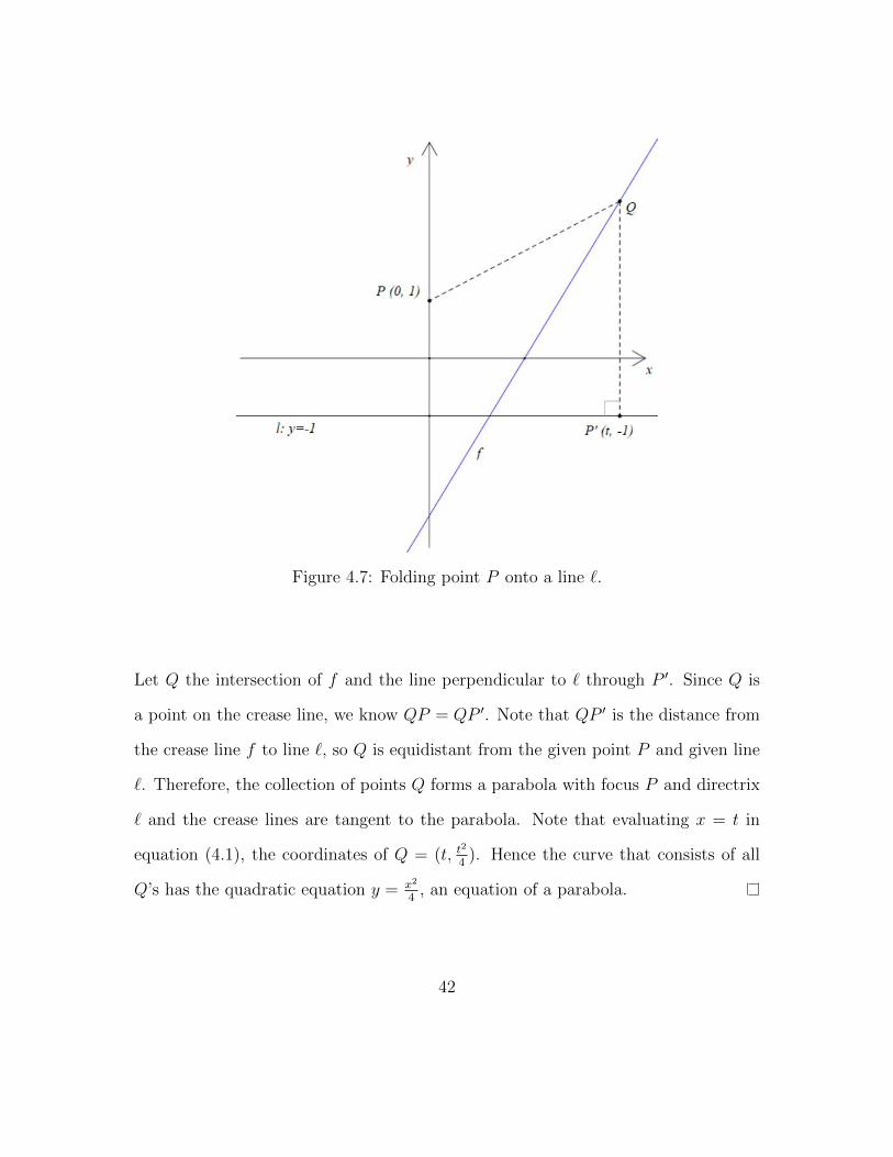
Figure 47 Folding point P onto a line `
Let Q the intersection of f and the line perpendicular to ` through P prime Since Q is
a point on the crease line we know QP = QP prime Note that QP prime is the distance from
the crease line f to line ` so Q is equidistant from the given point P and given line
` Therefore the collection of points Q forms a parabola with focus P and directrix
` and the crease lines are tangent to the parabola Note that evaluating x = t in
equation (41) the coordinates of Q = (t t2
4) Hence the curve that consists of all
Qrsquos has the quadratic equation y = x2
4 an equation of a parabola
42
Rearranging equation (41) and solving for t we have
t2
4minus t
2x+ y = 0rArr t =
x2plusmnradic
(x2)2 minus y
12
(42)
t has real values only when (x2)2 minus y ge 0 ie when y le x2
4 Specifically the points
on the parabola satisfy y = x2
4and all points P2 in the plane that can be hit by a
crease line must be y le x2
4 So O5 cannot happen when P2 is in the inside of the
parabola
Now we can use a parabola to construct square roots with origami
Corollary 435 The set of origami constructible numbers O is closed under taking
square roots4
Proof Given length r we will show thatradicr is origami-constructible Let P1 = (0 1)
and ` y = minus1 Let P2 = (0minus r4) Then using O5 fold P1 onto ` through P2
We know that the equation of our crease line is y = t2x minus t2
4 from equation (41)
from the proof of Theorem 434 Since this line has to pass p2 minus r4
= minus t2
4 so
t =radicr Therefore the point where p1 lands on ` will give us a coordinate of desired
length
Corollary 435 implies that C sube O In fact O is strictly larger than C from
O6 Recall O6 lsquoGiven two points p1 and p2 and two lines `1 and `2 we can fold a
line that places p1 onto `1 and p2 onto `2rsquo
4A geometric proof was made previously in Lemma 433
43
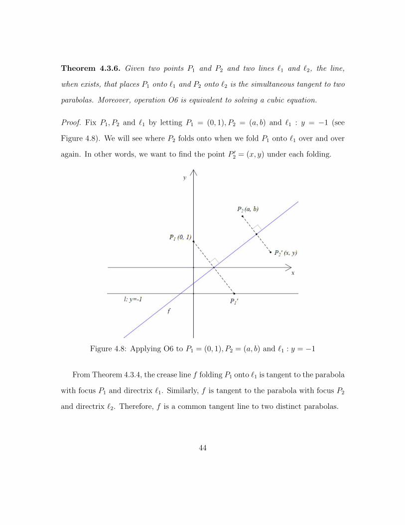
Theorem 436 Given two points P1 and P2 and two lines `1 and `2 the line
when exists that places P1 onto `1 and P2 onto `2 is the simultaneous tangent to two
parabolas Moreover operation O6 is equivalent to solving a cubic equation
Proof Fix P1 P2 and `1 by letting P1 = (0 1) P2 = (a b) and `1 y = minus1 (see
Figure 48) We will see where P2 folds onto when we fold P1 onto `1 over and over
again In other words we want to find the point P prime2 = (x y) under each folding
Figure 48 Applying O6 to P1 = (0 1) P2 = (a b) and `1 y = minus1
From Theorem 434 the crease line f folding P1 onto `1 is tangent to the parabola
with focus P1 and directrix `1 Similarly f is tangent to the parabola with focus P2
and directrix `2 Therefore f is a common tangent line to two distinct parabolas
44
Recall the equation of f is y = t2xminus t2
4 Since this line also folds P2 onto P prime2 it is
the perpendicular bisector of P2P prime2 The slope and midpoint between P2 onto P prime2 are
yminusbxminusa and (a+x
2 b+y
2) respectively Since P2P prime2 is perpendicular to f yminusb
xminusa = minus2t so
t
2= minus(
xminus ay minus b
) (43)
Also since f passes the midpoint of P2P prime2
y + b
2=t
2(a+ x
2)minus t2
4(44)
Substituting equation (43) into equation (44) we obtain
y + b
2= minus(
xminus ay minus b
)(a+ x
2)minus (
xminus ay minus b
)2
rArr (y + b)(y minus b)2 = minus(x2 minus a2)(y minus b)minus 2(xminus a)2
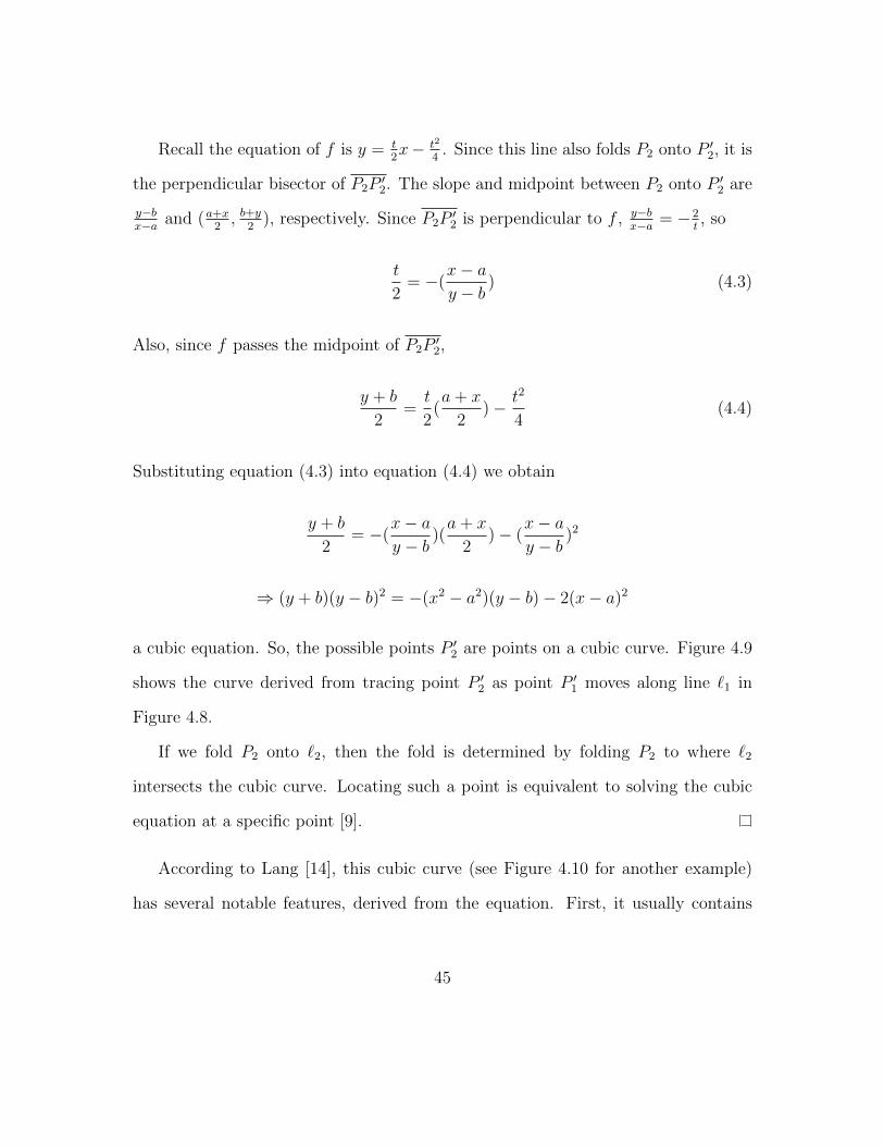
a cubic equation So the possible points P prime2 are points on a cubic curve Figure 49
shows the curve derived from tracing point P prime2 as point P prime1 moves along line `1 in
Figure 48
If we fold P2 onto `2 then the fold is determined by folding P2 to where `2
intersects the cubic curve Locating such a point is equivalent to solving the cubic
equation at a specific point [9]
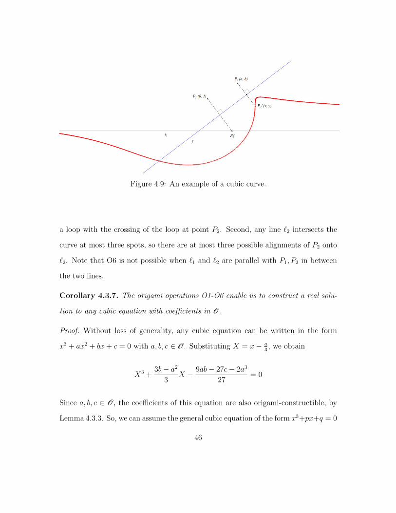
According to Lang [14] this cubic curve (see Figure 410 for another example)
has several notable features derived from the equation First it usually contains
45
Figure 49 An example of a cubic curve
a loop with the crossing of the loop at point P2 Second any line `2 intersects the
curve at most three spots so there are at most three possible alignments of P2 onto
`2 Note that O6 is not possible when `1 and `2 are parallel with P1 P2 in between
the two lines
Corollary 437 The origami operations O1-O6 enable us to construct a real solu-
tion to any cubic equation with coefficients in O
Proof Without loss of generality any cubic equation can be written in the form
x3 + ax2 + bx+ c = 0 with a b c isin O Substituting X = xminus a3 we obtain
X3 +3bminus a2
3X minus 9abminus 27cminus 2a3
27= 0
Since a b c isin O the coefficients of this equation are also origami-constructible by
Lemma 433 So we can assume the general cubic equation of the form x3+px+q = 0
46
Figure 410 An example of a cubic curve
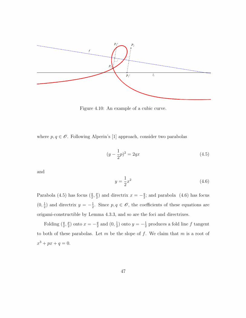
where p q isin O Following Alperinrsquos [1] approach consider two parabolas
(y minus 1
2p)2 = 2qx (45)
and
y =1
2x2 (46)
Parabola (45) has focus ( q2 p2) and directrix x = minus q
2 and parabola (46) has focus
(0 12) and directrix y = minus1
2 Since p q isin O the coefficients of these equations are
origami-constructible by Lemma 433 and so are the foci and directrixes
Folding ( q2 p2) onto x = minus q
2and (0 1
2) onto y = minus1
2produces a fold line f tangent
to both of these parabolas Let m be the slope of f We claim that m is a root of
x3 + px+ q = 0
47
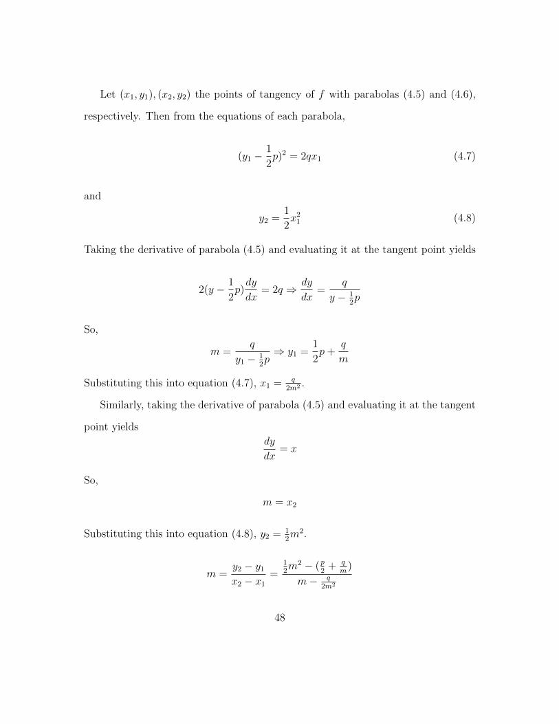
Let (x1 y1) (x2 y2) the points of tangency of f with parabolas (45) and (46)
respectively Then from the equations of each parabola
(y1 minus1
2p)2 = 2qx1 (47)
and
y2 =1
2x21 (48)
Taking the derivative of parabola (45) and evaluating it at the tangent point yields
2(y minus 1
2p)dy
dx= 2q rArr dy
dx=
q
y minus 12p
So
m =q
y1 minus 12prArr y1 =
1
2p+
q
m
Substituting this into equation (47) x1 = q2m2
Similarly taking the derivative of parabola (45) and evaluating it at the tangent
point yields
dy
dx= x
So
m = x2
Substituting this into equation (48) y2 = 12m2
m =y2 minus y1x2 minus x1
=12m2 minus (p
2+ q
m)
mminus q2m2
48
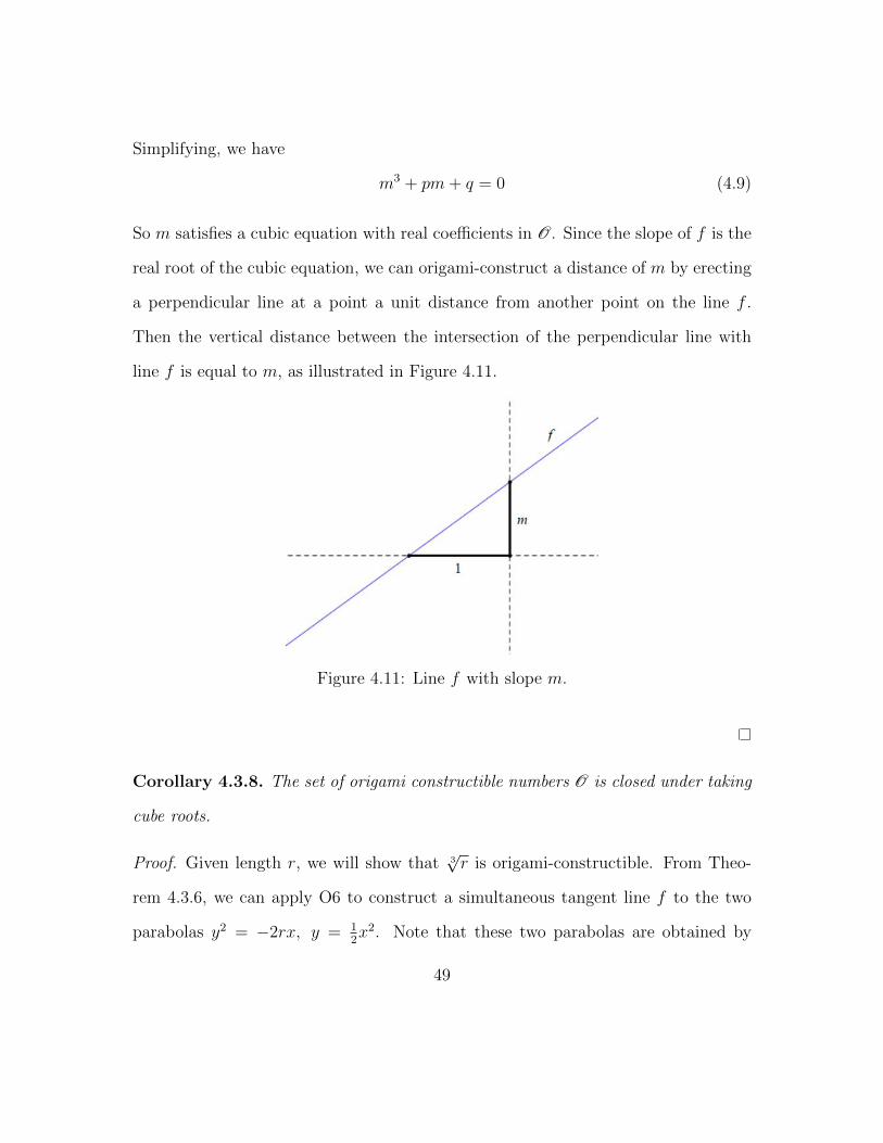
Simplifying we have
m3 + pm+ q = 0 (49)
So m satisfies a cubic equation with real coefficients in O Since the slope of f is the
real root of the cubic equation we can origami-construct a distance of m by erecting
a perpendicular line at a point a unit distance from another point on the line f
Then the vertical distance between the intersection of the perpendicular line with
line f is equal to m as illustrated in Figure 411
Figure 411 Line f with slope m
Corollary 438 The set of origami constructible numbers O is closed under taking
cube roots
Proof Given length r we will show that 3radicr is origami-constructible From Theo-
rem 436 we can apply O6 to construct a simultaneous tangent line f to the two
parabolas y2 = minus2rx y = 12x2 Note that these two parabolas are obtained by
49
setting p = 0 q = minusr for the two parabolas (45) and (46) in the proof of Corol-
lary 438 From equation 49 f has slope m = 3radicr so m = 3
radicr isin O
Theorem 439 Let r isin R Then r isin O if and only if there is a finite sequence of
fields Q = F0 sub F1 sub F2 sub middot middot middot sub Fn sub R such that r isin Fn and [Fi Fiminus1] = 2 or 3
for each 1 le i le n
Proof (rArr) Suppose r isin O As discussed in section 41 r isin O only when it
could be constructed through operations O1-O7 So far we have shown that origami
constructions in F involve a field extension of degree 1 2 or 3 From induction on
the number of constructions required to construct r there must be a finite sequence
of fields Q = F0 sub F1 sub middot middot middot sub Fn sub R such that r isin Fn with [Fi Fiminus1] = 2 or 3
(lArr) Suppose Q = F0 sub F1 sub F2 sub middot middot middot sub Fn sub R such that [Fi Fiminus1] = 2 or 3
Then Fi = Fiminus1[radicdi] or Fi = Fiminus1[
3radicdi] for some di isin Fi If n = 0 then r isin F0 = Q
and Q sub C from Lemma 433 Suppose any element of Fn is origami-constructible
for when n = k minus 1 Then any dk isin Fkminus1 is origami-constructible which implies
thatradicdk and 3
radicdk is also constructible from Corollary 435 and Corollary 438
Therefore any element of Fk = Fkminus1[radicdk] and Fk = Fkminus1[
3radicdk] is also origami-
constructible From mathematical induction any r isin Fn is origami-constructible
Corollary 4310 If r isin O then [Q(r) Q] = 2a3b for some integers a b ge 0
Proof From Theorem 439 if r isin O there is a finite sequence of fields Q = F0 sub
middot middot middot sub Fn sub R such that r isin Fn and for each i = 0 1 n [Fi Fiminus1] = 2 or 3 So
50
by the Tower Rule (Theorem 2210)
[Fn Q] = [Fn Fnminus1] middot middot middot [F1 F0] = 2k3l
with k + l = n Since Q sub Q(r) sub Fn again by the Tower Rule [Q(r) Q]|[Fn
Q] = 2k3l so if r isin O then [Q(r) Q] = 2a3b for some integers a b ge 0
44 Some Origami-constructible Objects
In Chapter 3 we have seen that straightedge and compass constructions can only
produce numbers that are solutions to equations with degree no greater than 2 In
other words quadratic equations are the highest order of equations straightedge and
compass can solve As a result trisecting an angle or doubling a cube was proved
impossible with straightedge and compass since they require producing lengths that
are solutions to cubic equations As shown above (Section 43) in addition to con-
structing what straightedge and compass can do origami can also construct points
that are solutions to cubic equations (from O6) Therefore doubling a cube and tri-
secting an angle is possible with origami Although we know that these constructions
could be done theoretically in the following I elaborate on the origami operations
through which one can double a cube or trisect any given angle
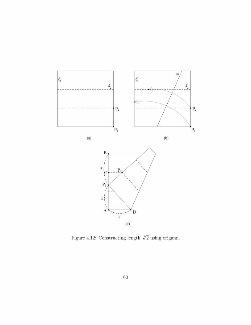
Theorem 441 (Doubling the cube) It is possible to construct an edge of a cube
double the volume of a given cube using origami
51
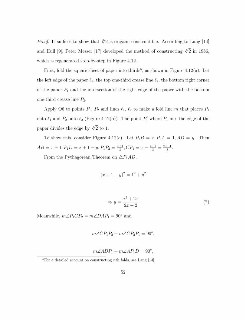
Proof It suffices to show that 3radic
2 is origami-constructible According to Lang [14]
and Hull [9] Peter Messer [17] developed the method of constructing 3radic
2 in 1986
which is regenerated step-by-step in Figure 412
First fold the square sheet of paper into thirds5 as shown in Figure 412(a) Let
the left edge of the paper `1 the top one-third crease line `2 the bottom right corner
of the paper P1 and the intersection of the right edge of the paper with the bottom
one-third crease line P2
Apply O6 to points P1 P2 and lines `1 `2 to make a fold line m that places P1
onto `1 and P2 onto `2 (Figure 412(b)) The point P prime1 where P1 hits the edge of the
paper divides the edge by 3radic
2 to 1
To show this consider Figure 412(c) Let P1B = x P1A = 1 AD = y Then
AB = x+ 1 P1D = x+ 1minus y P1P2 = x+13 CP1 = xminus x+1
3= 2xminus1
3
From the Pythagorean Theorem on 4P1AD
(x+ 1minus y)2 = 12 + y2
rArr y =x2 + 2x
2x+ 2()
Meanwhile mangP1CP2 = mangDAP1 = 90 and
mangCP1P2 +mangCP2P1 = 90
mangADP1 +mangAP1D = 90
5For a detailed account on constructing nth folds see Lang [14]
52
mangCP1P2 +mangAP1D = 90
So mangCP1P2 = mangADP1 and mangCP2P1 = mangAP1D Therefore 4P1CP2 sim
4DAP1 and thus
DA
DP1
=P1C
P1P2
rArr y
x+ 1minus y=
2xminus13
x+13
=2xminus 1
x+ 1
rArr x2 + 2x
x2 + 2x+ 2=
2xminus 1
x+ 1 from(lowast)
rArr x3 + 3x2 + 2x = 2x3 + 3x2 + 2xminus 2
rArr x3 = 2
So x = 3radic
2
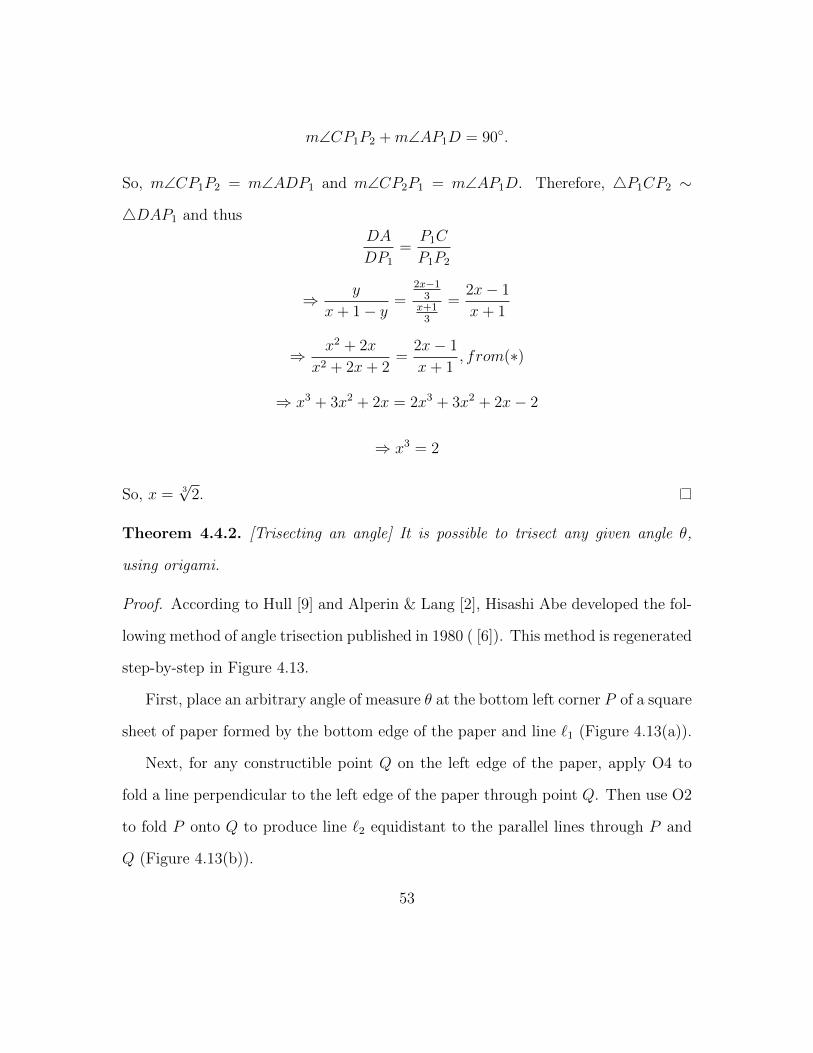
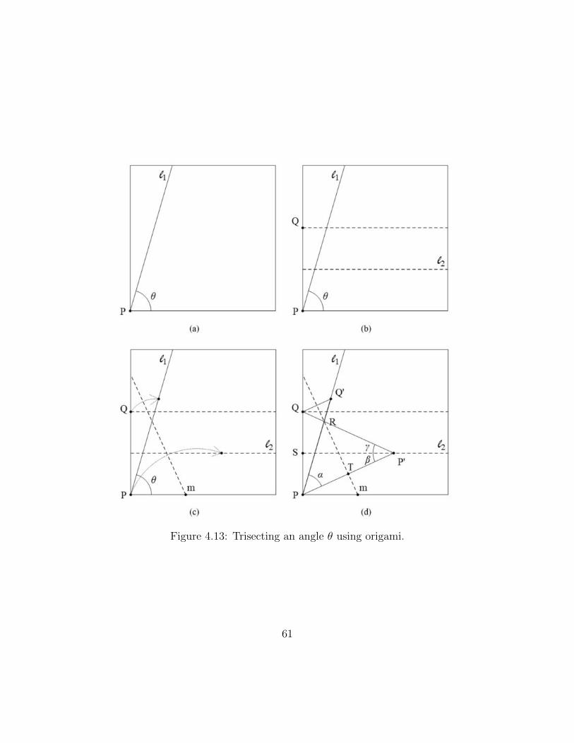
Theorem 442 [Trisecting an angle] It is possible to trisect any given angle θ
using origami
Proof According to Hull [9] and Alperin amp Lang [2] Hisashi Abe developed the fol-
lowing method of angle trisection published in 1980 ( [6]) This method is regenerated
step-by-step in Figure 413
First place an arbitrary angle of measure θ at the bottom left corner P of a square
sheet of paper formed by the bottom edge of the paper and line `1 (Figure 413(a))
Next for any constructible point Q on the left edge of the paper apply O4 to
fold a line perpendicular to the left edge of the paper through point Q Then use O2
to fold P onto Q to produce line `2 equidistant to the parallel lines through P and
Q (Figure 413(b))
53
Finally apply O6 to points PQ and lines `1 `2 to make a fold line m that places
P onto `2 and Q onto `1 (Figure 413(c)) The reflection of point P about line m say
P prime can be constructed as the intersection of the line perpendicular to m through P
and the line `2 (we can construct the reflection of point Q in a similar manner) The
angle formed by the bottom edge of the paper and segment PP prime has the measure of
θ3
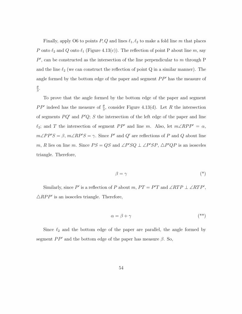
To prove that the angle formed by the bottom edge of the paper and segment
PP prime indeed has the measure of θ3 consider Figure 413(d) Let R the intersection
of segments PQprime and P primeQ S the intersection of the left edge of the paper and line
`2 and T the intersection of segment PP prime and line m Also let mangRPP prime = α
mangPP primeS = β mangRP primeS = γ Since P prime and Qprime are reflections of P and Q about line
m R lies on line m Since PS = QS and angP primeSQ perp angP primeSP 4P primeQP is an isosceles
triangle Therefore
β = γ ()
Similarly since P prime is a reflection of P about m PT = P primeT and angRTP perp angRTP prime
4RPP prime is an isosceles triangle Therefore
α = β + γ ()
Since `2 and the bottom edge of the paper are parallel the angle formed by
segment PP prime and the bottom edge of the paper has measure β So
54
θ = α + β
= (β + γ) + β from (lowastlowast)
= 3β from (lowast)
Note that the angle in Figure 413 has measures between 0 and π2 When the
angle has measure θ = π2 Q = Qprime and thus line m folds point P onto `2 through
point Q Since 4QPP prime is an equilateral triangle in this case segment PP prime trisects
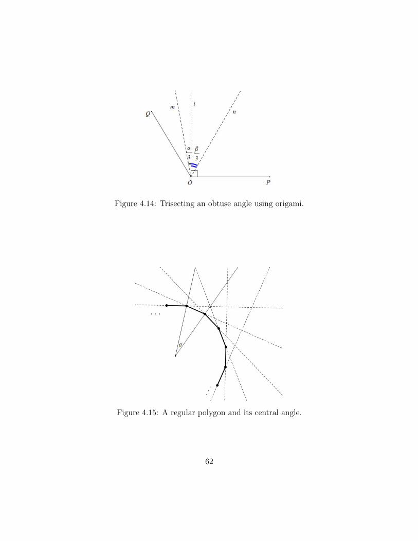
θ When the angle is obtuse the angle can be divided into an acute angle α and
a right angle β so θ = α + β This can be done by using O4 to construct a line `
perpendicular to one side of the angle through its center O (see Figure 414)
α
3+β
3=α + β
3=θ
3
So the angle between m (the trisection line of the acute angle) and n (the trisection
line of the right angle) give us the trisection of the obtuse angle Therefore the
above method of angle trisection can be applied to any arbitrary angle
45 Origami-constructible Regular Polygons
In this section we examine the regular n-gons that are origami-constructible For
the purpose of our discussion we expand the set R2 in which origami constructions
are made to C = a+ bi|a b isin R
We first define what an origami-constructible polygon is
55
Definition 451 An origami-constructible polygon is a closed connected plane
shape formed by a finite number of origami-constructible lines An origami-constructible
regular polygon is an origami-constructible polygon in which segments of the lines
form sides of equal length and angles of equal size
The vertices and interior angles of an origami-constructible polygon as inter-
sections of origami-constructible lines are also origami-constructible and the central
angle θ = 2πn
is constructible as the intersection of the bisector (apply O3) of two
consecutive interior angles (see Figure 415)
Before we determine which regular polygons are origami-constructible we define
splitting fields and cyclotomic extensions
Definition 452 Let F a field and f(x) isin F [x] Then the extension K of F
is called a splitting field for f(x) if f(x) factors completely into linear factors in
K[x] but does not factor completely into linear factors over any proper subfield of K
containing F
Proposition 453 For any field F if f(x) isin F [x] then there exists a splitting
field K for f(x) [5 p536]
Consider the polynomial xn minus 1 and its splitting field over Q Over C the poly-
nomial xnminus1 has n distinct solutions namely the nth roots of unity These solutions
can be interpreted geometrically as n equally spaced points along the unit circle
in the complex plane The nth roots of unity form a cyclic group generated by a
primitive nth root of unity typically denoted ζn
56
Definition 454 The splitting field of xn minus 1 over Q is the field Q(ζn) and it is
called the cyclotomic field of nth roots of unity
Proposition 455 The cyclotomic extension Q(ζn)Q is generated by the nth roots
of unity over Q with [Q(ζn) Q] = φ(n) where φ denotes Eulerrsquos φ-function6
Eulerrsquos φ-function in Proposition 453 is defined as the number of integers a
(1 le a lt n) that are relatively prime to n which is equivalent to the order of the
group (ZnZ)times According to Cox [4 p270] Eulerrsquos φ-function could be evaluated
with the formula
φ(n) = nprodp|n
(1minus 1
p) (410)
Definition 456 An isomorphism of a field K to itself is called an automorphism
of K Aut(K) denotes the collection of automorphisms of K If KF is an extension
field then define Aut(KF ) as the collection of automorphisms of K which fixes all
the elements of F
Definition 457 Let KF a finite extension If |Aut(KF )| = [K F ] then K is
Galois over F and KF is a Galois extension If KF is Galois Aut(KF ) is called
the Galois group of KF denoted Gal(KF )
Proposition 458 If K is the splitting field over F of a separable polynomial f(x)
then KF is Galois [5 p 562]
Therefore the cyclotomic field Q(ζn) of nth roots of unity is a Galois extension
of Q of degree φ(n) In fact
6For a detailed proof of Proposition 453 see [5 p 555]
57
Proposition 459 The Galois group Gal(Q(ζn)Q) sim= (ZnZ)times (see [5 p 596])
Theorem 4510 (Regular n-gon) A regular n-gon is origami-constructible if and
only if n = 2a3bp1 middot middot middot pr for some r isin N where each distinct pi is of the form
pi = 2c3d + 1 for some a b c d ge 0
Proof Suppose a regular n-gon is origami-constructible We can position it in our
Cartesian plane such that it is centered at 0 with a vertex at 1 Then the vertices of
the n-gon are the nth roots of unity which are origami-constructible On the other
hand if we can origami-construct the primitive nth root of unity ζn = e2πin we can
origami-construct all nth roots of unity as repeated reflection by applying O4 and
the addition of lengths (Figure 44) Then we can construct the regular n-gon by
folding lines through consecutive nth roots of unities Simply put a regular n-gon
is origami-constructible if and only if the primitive nth root of unity ζn is origami-
constructible Therefore it suffices to show that ζn is origami-constructible if and
only if n = 2a3bp1 middot middot middot pr where each pi are distinct Fermat primes for some r isin N
(rArr) Suppose ζn is origami-constructible From Corollary 4310 [Q(ζn) Q]
is a power of 2 or 3 and from Proposition 453 [Q(ζn) Q] = φ(n) Therefore
φ(n) = 2`3m for some `m ge 0 Let the prime factorization of n = qa11 middot middot middot qs1s where
qa11 middot middot middot qs1s are distinct primes and a1 middot middot middot as ge 1 Then from equation (410)
φ(n) = qa1minus11 (q1 minus 1) middot middot middot qasminus1s (qs minus 1)
and φ(n) = 2`3m only when each qi is either 2 or 3 or qiminus 1 = 2c3d for some c d ge 0
58
(lArr) Suppose n = 2a3bp1 middot middot middot pr for some r isin N where each distinct pi is of the
form pi = 2c3d + 1 for some a b c d ge 0 Then from equation (410)
φ(n) = 2a3bp1 middot middot middot pr(1minus1
2)(1minus 1
3)(1minus 1
p1) middot middot middot (1minus 1
pr)
= 2a3bminus1(p1 minus 1) middot middot middot (pr minus 1) = 2`3m
for some `m ge 0
If φ(n) = 2`3m then G = Gal(Q(ζn)Q) is an abelian group (from Proposi-
tion 459) whose order is a power of 2 or 3 Then we have a sequence of subgroups
1 = G0 lt G1 lt G2 lt middot middot middot lt Gn = G with each GiGiminus1 a Galois extension which is
cyclic of order 2 or 37 Hence from Theorem 439 ζn is origami-constructible
7From the Fundamental Theorem of Abelian Groups and the Fundamental Theorem of GaloisTheory [5 p158p574]
59
Figure 412 Constructing length 3radic
2 using origami
60
Figure 413 Trisecting an angle θ using origami
61
Figure 414 Trisecting an obtuse angle using origami
Figure 415 A regular polygon and its central angle
62
Chapter 5
Extensions of origami theory and
closing remarks
51 Extensions of origami theory
511 Additional tools
Several origami theorists have extended the traditional axiom set of single-fold op-
erations by allowing additional geometrical tools for construction
For example in [13] Kasem et al (2011) studied possible extensions of origami
using the compass Here the compass allows one to construct circles centered at
an origami point with radius a distance between two origami points Kasem et al
presented three new operations which they termed rdquoOrigami-and-Compass Axiomsrdquo
(p 1109) and showed that the expanded set of axioms allows one to construct
common tangent lines to ellipses or hyperbolas In addition they demonstrated a
new method for trisecting a given angle and explained that they provide an interesting
way of solving equations of degree 4 However according to Kasem et al combining
63
the use of the compass with origami does not increase the construction power of
origami beyond what is constructible by the traditional axiom set
In [7] Ghourabi et al (2013) took a similar approach by introducing fold opera-
tions that produce conic sections into origami Specifically Ghourabi et al presented
one additional fold operation which superimposes one point onto a line and another
point onto a conic section Ghourabi et al proved that the new extended set of
fold operations generate polynomials of degree up to six They left the question
of whether these fold operations solve all 5th and 6th degree equations for future
research
512 An eighth axiom
In his paper [15] Lucero revisited the single-fold operations by viewing folding as
the geometry of reflections After enumerating all possible incidences between con-
structible points and lines on a plane induced by a reflection Lucero derived 8
possible fold operations that satisfy all combinations of incidences The eight ax-
ioms included seven of the traditional axioms and one new operation which is to
fold a constructible line such that it folds onto itself As a practical solution to allow
one to fold one layer along a line marked on the other layer Lucero introduced the
additional single-fold operation as needed for the completeness of the axioms and
application in practical origami
64
513 Beyond the single fold
In [2] Alperin and Lang (2009) extended the traditional axiom set of single-fold op-
erations by allowing alignments of points and lines along multiple folds For example
a two-fold alignment is an alignment of points or lines with two simultaneous fold
creases As an example of a two-fold alignment Alperin and Lang refer to Abersquos so-
lution (in 442) as a two-fold alignment combining O2 and O6 Since this alignment
can be partitioned into two sets each of which is a single-fold this two-fold align-
ment is called separable Enumerating on non-separable alignments Alperin and
Lang identified a unique set of 17 two-fold alignments which produce 489 distinct
two-fold operations Here Alperin and Lang restricted to two-fold axioms to those
that are non-separable and consist of fold linesldquoon a finite region of the Euclidean
plane with a finite number of solutionsrdquo (p 9) With the extended set of axioms
Alperin and Lang explained ldquoEach two-fold alignment yields a system of four equa-
tions in four variables with each equation of degree at most 4rdquo (p 14) but that not
all degree 4 polynomials can be produced Similarly Alperin and Lang explained
that some quintic polynomials can be solved by two-fold axioms but not in general
Alperin and Lang acknowledged the limitation in physically carrying out the two-
fold operations For one to create a two-fold alignment requires smooth variation of
the position of both folds until all alignments are satisfied which could be prac-
tically difficult Putting such limitations aside Alperin and Lang investigated the
construction power of origami when multi-fold operations are allowed For example
they showed that a 3-fold alignment of 3 simultaneous folds allows solving the general
65
quintic equation and more generally the general nth degree equation can be solved
with n-2 simultaneous folds
As such there are many extensions that have been studied Propose some addi-
tional extensions to think about here and think about the implications
52 Future research questions
In this section I pose questions about other possible extensions of origami theory
for future research
521 Allowing tracing
In [15] Lucero (2017) claimed ldquoIn origami mathematics it is assumed that all lines
and points marked on one layer are also defined on the layers above and below as if
the paper were lsquotransparentrsquordquo (p12) However such claim does not seem compatible
with the definition of a single-fold (A single-fold refers to folding the paper once
a new fold can only be made after the paper is unfolded) nor does it seem feasible
when considering actual paper folding of non-transparent paper Related to such
extension one question I pose is What implications can tracing have on origami
constructions In other words if one is allowed to construct a line or point by
tracing another line or point onto the paper when the paper is folded would that
change the set of origami-constructible numbers
66
522 Allowing cutting
Typically in origami cutting is not allowed As another possible extension of origami
theory I pose the question of what happens if cutting is allowed In order to explore
this idea there will need to be some specification of what cutting refers to and what
type of folds are allowed after the paper is cut For example we can consider a
case when one is allowed to cut the paper along lines or line segments connecting
two origami-constructible points In the case the paper is cut along a line into two
separable parts we can think of placing one part on top of the other and superimpos-
ing constructible points and lines from one layer onto the other (similar to tracing)
In the case the paper is cut along a line segment but not fully separated into two
parts then we can think of various ways one can fold the paper about the cut For
instance what can we do if the paper is cut along one of its edges What can we do
if there is a slit inside of the sheet of paper In such cases what would the set of
origami-constructible numbers look like
523 Starting with additional givens other than the unit
distance
Finally future research can investigate different types of field extensions derived
from origami constructions with different initial givens For example in origami
constructions we start with two points and a unit distance as initials What if we
start with three points instead of two with the collection of distances andor angles
given by these points not obtainable by only two points some unit distance apart
67
53 Closing remarks
In this thesis I presented an exposition of origami constructible objects and its
associated algebraic field I introduced what origami is reviewed the basic def-
initions and theorems of field theory that were used in the thesis discussed the
more commonly known straightedge and compass constructions introduced the ba-
sic single-fold operations of origami and discussed what it means for an object to be
origami-constructible showed how to prove or disprove the constructibility of some
origami objects and finally presented some additional thoughts for future studies
68
Bibliography
[1] Roger C Alperin A mathematical theory of origami constructions and numbers
New York J Math 6(119)133 2000
[2] Roger C Alperin and Robert J Lang One- two- and multi-fold origami axioms
In Origami4 pages 371ndash393 A K Peters Natick MA 2009
[3] David Auckly and John Cleveland Totally real origami and impossible paper
folding Amer Math Monthly 102(3)215ndash226 1995
[4] David A Cox Galois theory Pure and Applied Mathematics (Hoboken) John
Wiley amp Sons Inc Hoboken NJ second edition 2012
[5] David S Dummit and Richard M Foote Abstract algebra John Wiley amp Sons
Inc Hoboken NJ third edition 2004
[6] Koji Fusimi Trisection of angle by abe Saiensu supplement 8 1980
[7] Fadoua Ghourabi Asem Kasem and Cezary Kaliszyk Algebraic analysis of
huzitarsquos origami operations and their extensions Automated Deduction in Ge-
ometry (9783642406713) page 143 2013
[8] Koshiro Hatori Krsquos origami Origami construction httpwwwjadedtine
jp~hatorilibraryconstehtml2003 Accessed 2017-07-08
69
[9] Thomas Hull Project origami A K Peters Ltd Wellesley MA first edition
2006 Activities for exploring mathematics
[10] Humiaki Huzita Axiomatic development of origami geometry In Proceedings of
the First International Meeting of Origami Science and Technology 1989 pages
143ndash158 1989
[11] Humiaki Huzita Understanding geometry through origami axioms In Proceed-
ings of the First International Conference on Origami in Education and Therapy
(COET91) pages 37ndash70 British Origami Society 1992
[12] Jacques Justin Resolution par le pliage de lrsquoequation du troisieme degre et
applications geometriques In Proceedings of the first international meeting of
origami science and technology pages 251ndash261 Ferrara Italy 1989
[13] Asem Kasem Fadoua Ghourabi and Tetsuo Ida Origami axioms and circle
extension In Proceedings of the 2011 ACM Symposium on Applied Computing
SAC rsquo11 pages 1106ndash1111 New York NY USA 2011 ACM
[14] Robert J Lang Origami and geometric constructions Self Published (1996
2003) 1996
[15] Jorge C Lucero On the elementary single-fold operations of origami Reflections
and incidence constraints on the plane In Forum Geometricorum volume 17
pages 207ndash221 2017
[16] George E Martin Geometric constructions Undergraduate Texts in Mathe-
matics Springer-Verlag New York 1998
70
[17] Peter Messer Problem 1054 Crux Mathematicorum 12(10)284ndash285 1986
[18] Mathematics Origami in Science and Education The 6th international
meeting on origami science mathematics and education program and ab-
stracts httporigamigrjp6osmeprogram6OSME-Abstracts2014pdf
Retrieved 2017-07-08
71
Appendix List of Geometric
Symbols
larrrarrAB line through two points A and B
minusrarrAB ray with endpoint A that passes through B
AB segment connecting two points A and B
AB distance between A and B
angABC angle with vertex B with raysminusrarrBA and
minusminusrarrBC
mangABC measure of angABC
4ABC triangle with vertices A B C
ABC area of 4ABC
ABCD quadrilateral with edges AB BC CD DA
p sim= q p congruent to q
p sim q p similar to q
72
ORIGAMI-CONSTRUCTIBLE NUMBERS
by
HWA YOUNG LEE
BS Ewha Womans University 2004
MEd Ewha Womans University 2009
PhD University of Georgia 2017
A Thesis Submitted to the Graduate Faculty
of The University of Georgia in Partial Fulfillment
of the Requirements for the Degree
MASTER OF ARTS
Athens Georgia
2017
ccopy2017
Hwa Young Lee
All Rights Reserved
ORIGAMI-CONSTRUCTIBLE NUMBERS
by
HWA YOUNG LEE
Major Professor Daniel Krashen
Committee Robert RumelyPete Clark
Electronic Version Approved
Suzanne BarbourDean of the Graduate SchoolThe University of GeorgiaDecember 2017
Acknowledgments
First I would like to thank all the math teachers and students I had and have
Without these people I would not be here I would also like to thank my advisor
and committee members who provided valuable feedback and support Dr Krashen
thank you for your mentorship patience assistance with technology and creativity
that sparked many ideas for this thesis Dr Rumely thank you for all the origami
books you let me borrow and for our chats about origami both were very helpful
Dr Clark thank you for your advisement and support in pursuing this degree and
for happily joining my committee Additionally I would like to thank my family
and friends for their love and support which gave me the strength to continue my
graduate studies Finally I would like to give a special acknowledgement to my dear
friend Irma Stevens who was always willing to give me advice and help when writing
this thesis
iv
Contents
Acknowledgements iv
List of Figures vii
List of Tables viii
1 Introduction 1
11 Geometric Constructions 1
12 Origami Constructions 3
13 Overview of Thesis Chapters 5
2 Preliminaries in Field Theory 6
21 Basic Definitions 6
22 Field Theory 8
3 Straightedge and Compass Constructions 14
31 Initial Givens Operations and Basic Constructions 14
32 Constructible Numbers 17
33 Impossibilities 26
34 Marked Rulers and Verging 28
v
4 Origami Constructions 31
41 Initial Givens and Single-fold Operations 31
42 Origami Constructions 35
43 Origami-constructible Numbers 36
44 Some Origami-constructible Objects 51
45 Origami-constructible Regular Polygons 55
5 Extensions of origami theory and closing remarks 63
51 Extensions of origami theory 63
52 Future research questions 66
53 Closing remarks 68
Bibliography 69
Appendix 72
vi
List of Figures
31 Three basic straightedge and compass constructions 16
32 Two straightedge and compass constructions starting with given length
r 18
33 The construction of n isin Z 19
34 Constructing lengths ab ab and
radica 20
35 Verging through P with respect to ` and m 28
36 Trisecting an angle with marked ruler and compass 29
37 Proving angle trisection with marked ruler and compass 30
41 Single-fold operations of origami 33
42 E2prime Constructing a line parallel to ` through P with origami 36
43 Constructing the axes and point (0 1) 37
44 Constructing length a+ b using origami 39
45 Constructing lengthradica using origami 40
46 Lines folding point P onto line ` 41
47 Folding point P onto a line ` 42
48 Applying O6 to P1 = (0 1) P2 = (a b) and `1 y = minus1 44
49 An example of a cubic curve 46
410 An example of a cubic curve 47
vii
411 Line f with slope m 49
412 Constructing length 3radic
2 using origami 60
413 Trisecting an angle θ using origami 61
414 Trisecting an obtuse angle using origami 62
415 A regular polygon and its central angle 62
viii
Chapter 1
Introduction
11 Geometric Constructions
There are various tools such as the straightedge and compass one can use to con-
struct geometric objects Each construction tool has its unique rules of operating
when making geometric constructions To construct a geometric object means to
carry out a set of operations the tool permits that collectively produce the geometri-
cal object Note that constructing a geometric object differs from making a freehand
illustration or drawing of the object
Take the classical straightedge and compass as an example In straightedge and
compass constructions one can use either tool but not both simultaneously The
straightedge can only be used to draw the line through two given points but cannot
be used to measure length The compass can be used to construct a circle or arc with
a given center and point on the circle or arc Some basic straightedge and compass
constructions will be discussed in Chapter 3 (see Figures 31 and32)
1
The system of assumptions or axioms concerning the unique rules of operating for
each tool have a profound effect on what objects are constructible within a particular
framework While the classical framework of straightedge and compass constructions
(described below) is better known one can expand this framework by adding other
constructions (for example see Section 34 on the marked ruler and verging) or
one can consider new frameworks such as constructions by origami which will be
explored later in detail
The straightedge and compass the rules of construction and the study of con-
structible objects go back to the ancient Greeks and Egyptians For example con-
sider the famous Greek geometry problems
Using only straightedge and compass
1 (Doubling a cube) Is it possible to construct a cube whose volume is equivalent
to twice the volume of a given cube
2 (Trisecting an angle) Is it possible to trisect any given angle of measure θ
3 (Squaring a circle) Is it possible to construct a square whose area is equivalent to
that of a given circle
The study of constructible objects including the famous Greek geometry problems
emerged from everyday life such as in architecture and surveying [14] For example
according to Cox [4 page 266] there are two versions of the origin of doubling a cube
King Minos and the tomb of his son the cubical altar of Apollo in Athens Both
involved the construction of some architectural structure Although straightedge
and compass may have lost their place in our everyday lives geometric constructions
2
with straightedge and compass are still introduced in high school geometry providing
opportunities for students to better understand definitions and characteristics of
geometric figures
Going back to the Greek geometry problems the Greeks were not able to solve
the famous geometry problems at that time but the search for solutions led to other
mathematical creations (eg Hippocrates of Chios and the lune Hippias of Elis
and the quadratrix Menaechmus and parabolas the spiral of Archimedes) [4] In
1837 Wantzel showed that trisecting an angle and doubling a cube by straightedge
and compass were not always possible in 1882 Lindemann showed that squaring
the circle was impossible with straightedge and compass when he showed that π is
transcendental over Q [4] The proofs will be discussed in Chapter 3
The development of Modern algebra and coordinate geometry played a big role in
solving these problems and studying geometric constructions with other various tools
such as the marked ruler divider Origami (paperfolding) and Mira Specifically
the collection of lengths that various geometric tools can theoretically construct
became associated with various algebraic fields Among the various tools of geometric
constructions this thesis presents an exposition of origami constructible objects and
its associated algebraic field
12 Origami Constructions
Origami is the Japanese art of paper folding in which one starts with a square-
shaped sheet of paper and folds it into various three-dimensional shapes Typically
3
in origami one starts with an unmarked square-shaped sheet of paper using only
folding (usually cutting is not allowed) with the goal of constructing reference points
that are used to define folds that produce the final object [14] Reference points
can be points on the square-shaped papers (eg the four corners) but also can be
generated as intersections of lines formed by the edges of the paper or creases that
align a combination of points edges and creases [14]
Although origami originally started as an activity in everyday life origami has
become a topic of research According to Lang [14 page 42] ldquoStarting in the 1970s
several folders began to systematically enumerate the possible combinations of folds
to study what types of distances were constructible by combining them in various
waysrdquo In the 1980s several researchers identified a fixed set of well-defined folds
one can make in origami constructions (see Figure 41) and formalized the modern
study of geometric constructions with origami
In origami theory starting with the fixed set of well-defined folds researchers
have investigated the objects possible or impossible to construct using origami For
example it was shown that trisecting an angle and doubling a cube are possible
with origami constructions however constructing the regular 11-gon or solving the
general quintic equation was shown impossible [2]
There is an international conference lsquoThe International Meeting on Origami Sci-
ence Mathematics and Educationrsquo at which the origami community have gathered
since 1989 to discuss origami in science mathematics education technology and
art [18] With the development of the computer computational systems of origami
simulation have been developed and a more systematic study of origami has evolved
4
Origami has also been applied to other fields such as science and technology Ac-
cording to Lucero [15] the application of origami can be found in aerospace and
automotive technology materials science computer science biology civil engineer-
ing robotics and acoustics However as folding techniques have been adapted in
industry more rigor and formalization of origami theory has been called for For
example Kasem et al [13] and Ghourabi et al [7] called for more precise statements
of the folding operations and introduced the extension of origami constructions with
an additional tool of the compass
13 Overview of Thesis Chapters
In Chapter 2 I will first review the basic definitions and theorems of field theory
that will be used in subsequent chapters In Chapter 3 I will discuss the more com-
monly known straightedge and compass constructions as a lead into the discussion
on origami constructions In Chapter 4 I will introduce the basic single-fold opera-
tions of origami and discuss what it means for an object to be origami-constructible
Through algebraizing geometric constructions with origami I will show how to prove
or disprove the constructibility of some objects In Chapter 5 I end this thesis with
closing remarks and some additional thoughts for future studies
5
Chapter 2
Preliminaries in Field Theory
In this Chapter 2 I will review the basic definitions and theorems of field theory
that will be used in subsequent chapters
21 Basic Definitions
Definition 211 (Group) A group G is a set together with a binary operation
(usually denoted by middot and called the group operation) that satisfy the following
(i) (a middot b) middot c = a middot (b middot c) for all a b c isin G (Associativity)
(ii) There exists an element e isin G (called the identity of G) such that amiddote = emiddota = a
for all a isin G (Identity)
(iii) For each a isin G there exists an element aminus1 isin G (called the inverse of a) such
that a middot aminus1 = aminus1 middot a = e (Inverse)
The group G is called abelian if a middot b = b middot a for all a b isin G
6
Definition 212 (Subgroup) Given a group G a subset H of G is a subgroup of
G (denoted H le G) if H is nonempty and closed under multiplication and inverse
ie a b isin H rArr ab isin H and aminus1 isin H
Whereas the theory of groups involves general properties of objects having an
algebraic structure defined by a single binary operation the theory of rings involves
objects having an algebraic structure defined by two binary operations related by
the distributive laws [5 p222]
Definition 213 (Ring) A ring R is a set together with two operations +times
(addition and multiplication) that satisfy the following
(i) R is an abelian group under addition (denote the additive identity 0 and additive
inverse of element a as minusa)
(ii) (atimes b)times c = atimes (btimes c) for all a b c isin R (Multiplicative associativity)
(iii) (a + b) times c = (a times c) + (b times c) and a times (b + c) = (a times b) + (a times c) for all
a b c isin R (Left and right distributivity)
(iv) There exists an element 1 isin R (called the multiplicative identity) such that
1times a = atimes 1 = a for all a isin R (multiplicative unit)
Rings may also satisfy optional conditions such as
(v) atimes b = btimes a for all a b isin R
In this case the ring R is called commutative
7
(vi) For every a isin R 0 there exists an element aminus1 isin R such that a times aminus1 =
1 = aminus1 times a
In this case the ring R is called a division ring
Definition 214 (Subring) Given a ring R a subset S of R is a subring of R if
S is a subgroup of R closed under multiplication and if 1 isin S In other words S is
a subring of R if the operations of addition and multiplication in R restricted to S
give S the structure of a ring
A commutative division ring (a ring that satisfies all conditions (i) through (vi)
in Definition 213) is called a field More concisely
Definition 215 (Field) A field is a set F together with two binary operations +
and middot that satisfy the following
(i) F is an abelian group under + (with identity 0)
(ii) Ftimes = F minus 0 is an abelian group under middot (with identity 1)
(iii) a middot (b+ c) = (a middot b) + (a middot c) for all a b c isin F (Distributivity)
For example any set closed under all the arithmetic operations +minustimesdivide (divi-
sion by nonzero elements) is a field
22 Field Theory
Of particular interest in this thesis is the idea of extending a given field into a
(minimally) larger field so that the new field contains specific elements in addition
to all the elements of the given field We first define a field extension
8
Definition 221 If K is a field with subfield F then K is an extension field of
F denoted KF (read ldquoK over F rdquo) If KF is a field extension then K is a vector
space over F with degree dimFK denoted [K F ] The extension is finite if [K F ]
is finite and infinite otherwise
Definition 222 If K is an extension of field F and if α β middot middot middot isin K then the
smallest subfield of K containing F and α β middot middot middot isin K is called the field generated
by α β middot middot middot over F denoted F (α β middot middot middot ) An extension KF is finitely generated
if there are finitely many elements α1 αk isin K such that K = F (α1 αk) If
the field is generated by a single element α over F then K is a simple extension
of F with α a primitive element for the extension K = F (α)
We are specifically interested in field extensions that contain roots of specific
polynomials over a given field with the new field extending the field The following
propositions of such field extensions are taken as given without proof1
Proposition 223 Given any field F and irreducible polynomial p(x) isin F [x] there
exists an extension of F in which p(x) has a root Namely the field K = F [x](p(x))
in which F [x](p(x)) is the quotient of the ring F [x] by the maximal ideal (p(x))
Further if deg(p(x)) = n and α isin K denotes the class of x modulo p(x) then
1 α α2 αnminus1 is a basis for K as a vector space over F with [K F ] = n so
K = a0 + a1α + middot middot middot+ anminus1αnminus1|a0 anminus1 isin F
1For a detailed proof of these statements see Dummit amp Foote [5 pp 512-514]
9
While Proposition 223 states the existence of an extension field K of F that
contains a solution to a specific equation the next proposition indicates that any
extension of F that contains a solution to that equation has a subfield isomorphic to
K and that K is the smallest extension of F (up to isomorphism) that contains such
a solution
Proposition 224 Given any field F and irreducible polynomial p(x) isin F [x] sup-
pose L is an extension field of F containing a root α of p(x) and let F (α) denote the
subfield of L generated over F by α Then F (α) sim= F [x](p(x)) If deg(p(x)) = n
then F (α) = a0 + a1α + a2α2 + middot middot middot+ anminus1α
nminus1|a0 a1 anminus1 isin F sube L
Example 225 Consider F = R and p(x) = x2 + 1 an irreducible polynomial over
R Then we obtain the field K = R(x2 +1) sim= R(i) sim= R(minusi) an extension of R that
contains the solution of x2 + 1 = 0 [K F ] = 2 with K = a+ bi|a b isin R = C
The elements of a field extension K of F need not always be a root of a polynomial
over F
Definition 226 Let K be an extension of a field F The element α isin K is alge-
braic over F if α is a root of some nonzero polynomial f(x) isin F [x] If α isin K is
not the root of any nonzero polynomial over F then α is transcendental over F
The extension KF is algebraic if every element of K is algebraic over F
Proposition 227 Let K be an extension of a field F and α algebraic over F Then
there is a unique monic irreducible polynomial mα(x) isin F [x] with α as a root This
polynomial mα(x) is called the minimal polynomial for α over F and deg(mα) is
the degree of α So F (α) sim= F [x](mα(x)) with [F (α) F ] = deg(mα(x)) = degα
10
Proposition 228 If α is algebraic over F ie if α is a root to some polynomial
of degree n over F then [F (α) F ] le n On the other hand if [F (α) F ] = n
then α is a root of a polynomial of degree at most n over F It follows that any finite
extension KF is algebraic
Example 229 (Quadratic Extensions over F with char(F ) 6= 2) Let K an ex-
tension of a field F with the char(F ) 6= 22 and [K F ] = 2 Let α isin K but
α isin F Then α must be algebraic ie a root of a nonzero polynomial over F of
degree at most 2 by Proposition 228 Since α isin F this polynomial cannot be
of degree 1 Hence by Proposition 227 the minimal polynomial of α is a monic
quadratic mα(x) = x2 + bx + c with b c isin Q F sub F (α) sube K and [K F ] = 2 so
K = F (α) (see Proposition 227 and 228) From the quadratic formula (possible
since char(F ) 6= 2) the elements
minusbplusmnradicb2 minus 4c
2isin F (
radicd)
are roots of mα(x) with d = b2 minus 4c We can by Proposition 227 identify F (α)
with a subfield of F (radicd) by identifying α with 1
2(minusbplusmn
radicd) (either sign choice works)
We know that d is not a square in F since α isin F By construction F (α) sub F (radicd)
On the other handradicd = ∓(b + 2α) isin F (α) so F (
radicd) sube F (α) Therefore F (α) =
F (radicd) As such any extension K of F of degree 2 is of the form F (
radicd) where
d isin F is not a square in F Conversely any extension of the form F (radicd) where
2The characteristic of a field F is the smallest integer n such that n middot 1F = 0 If such n does notexist then the characteristic is defined to be 0
11
d isin F is not a square in F is an extension of degree 2 over F Such an extension is
called a quadratic extension over F
Particularly when F = Q any extension K of Q of degree 2 is of the form Q(radicd)
where 0 lt d isin Q is not a square in Q Conversely any extension of the form Q(radicd)
where 0 lt d isin Q is not a square in Q is an extension of degree 2 over Q Such an
extension is called a quadratic extension over Q
Theorem 2210 (Tower Rule) Let F a field extension of E and K a field extension
of F Then K is a field extension of E of degree [K E] = [K F ][F E]
Proof Suppose [F E] = m and [K F ] = n are finite Let α1 αm a basis for F
over E and β1 βn a basis for K over F Let β any element of K Since β1 βn
are a basis for K over F there are elements b1 bn isin F such that
β = b1β1 + b2β2 + middot middot middot+ bnβn (21)
Since α1 αm are a basis for F over E there are elements ai1 ain isin E i =
1 2 m such that each
bi = ai1α1 + ai2α2 + middot middot middot+ ainαn (22)
Substituting (22) into (22) we obtain
β =nsumj=1
msumi=1
aij(αiβj) aij isin F (23)
12
In other words any element of K can be written as a linear combination of the nm
elements αiβj with coefficients in F Hence the vectors αiβj span K as a vector space
over E
Suppose β = 0 in (23)
β =nsumj=1
msumi=1
aij(αiβj) =nsumj=1
(msumi=1
aijαi
)βj
Since β1 βn are linearly independentsumm
i=1 aijαi = 0 for all j = 1 n Since
α1 αm are linearly independent aij = 0 for all i = 1 2 m and j = 1 n
Therefore the nm elements αiβj are linearly independent over E and form a basis
for K over E Therefore [K E] = nm = [K F ][F E] If either [K F ] or [F E]
is infinite then there are infinitely many elements of K or F respectively so [K E]
is also infinite On the other hand if [K E] is infinite then at least one of [K F ]
and [F E] has to be infinite since if they are both finite the above proof shows that
[K E] is finite
13
Chapter 3
Straightedge and Compass
Constructions
To investigate the constructability of geometric objects using straightedge and com-
pass such as the problems posed by the Greeks we translate geometric construc-
tions into algebraic terms In this chapter we explore geometric constructions with
straightedge and compass and constructible numbers
31 Initial Givens Operations and Basic Construc-
tions
In straightedge and compass constructions two points say O and P are initially
given Starting with these given points we can carry out the following operations
with straightedge and compass which produce lines and circles
Operations of straightedge and compass constructions
Given two constructed points we can
14
C1 construct the line connecting the two points or
C2 construct a circle centered at one point and passing through the other point
We can also construct the intersection of constructed lines or circles which gives new
points
P1 We can construct the point of intersection of two distinct lines
P2 We can construct points of intersection of a line and a circle
P3 We can construct points of intersection of two distinct circles
Repeating C1 C2 with P1 P2 P3 on OP produces more constructible points
A constructible point is any point one can construct in a finite number of steps of
combinations of C1 C2 P1 P2 or P3
Examples of basic straightedge and compass constructions
Recall the following basic constructions in Figure 31 from high school geometry
For example to construct the perpendicular line through point P (see E1 in Fig-
ure 31) construct a circle of some radius centered at point P and let Q1 and Q2
be the two intersection points of the circle with ` Next construct circles centered
at Q1 and Q2 respectively whose radius is the distance between Q1 and Q21 These
two circles will intersect in two new points R1 and R2 The line through R1 and R2
passes through P and is perpendicular to `
Given points PQ and line ` with P isin ` and Q isin l to construct a line parallel
to ` through P (see E2 in Figure 31) construct a circle of some radius centered at
1The radius can be any length greater than half the distance between Q1 and Q2 to allow thetwo circles to intersect
15
Figure 31 Three basic straightedge and compass constructions
Q on ` and construct a circle centered at point P with same radius Construct line
m through P and Q and let the intersection of the circle centered at Q with m S
and the intersection of the circle centered at P with m U Let the intersection of the
circle centered at Q with ` R and construct a circle centered at S through R Then
construct another circle with same radius centered at U Let the intersection of the
circle centered at P and the circle centered at U T The line through P and T is
parallel to ` through P
To construct the angle bisector (see E3 in Figure 31) construct a circle of some
radius centered at the point O of intersection of the two lines Let S1 and S2 be the
two intersection points of the circle with the two sides ` and m respectively Next
construct two congruent circles of some radius centered at S1 and S2 respectively
16
Let point T one of the two intersections of the two circles The line through O and
T bisects the angle between lines ` and m These examples will be useful later
32 Constructible Numbers
Now we translate geometric distances obtained through constructions into algebraic
terms by associating lengths with elements of the real numbers Given a fixed unit
distance 1 we determine any distance by its length 1r = r1 isin R
Definition 321 A real number r is constructible if one can construct in a
finite number of steps two points which are a distance of |r| apart
The set of real numbers that are associated with lengths in R obtained by straight-
edge and compass constructions together with their negatives are constructible el-
ements of R Henceforth we do not distinguish between constructible lengths and
constructible real numbers
Given a constructible number r we can construct various objects using straight-
edge and compass Figure 32 shows two examples For example given a con-
structible number r we can construct an equilateral triangle with side length r as
follows First let A and B two points a distance of r apart Next construct circle
c1 centered at A with radius r and circle c2 centered at B with radius r Let C the
intersection of circles c1 c2 Then 4ABC is an equilateral triangle
Given the plane in which straightedge and compass constructions are made we
establish a coordinate system by taking point O as the origin and the distance be-
tween O and P as the unit length 1 Applying C1 to O and P we can construct the
17
Figure 32 Two straightedge and compass constructions starting with given lengthr
x-axis Applying E1 to the x-axis and point O we can construct the y-axis Then
the coordinates of the two given points O and P are (0 0) and (1 0) respectively
on the Cartesian plane As such using our points O and P we can construct a
coordinate system in the plane and use this to represent our points as ordered pairs
ie elements of R22 We then have
Lemma 322 A point (a b) isin R2 is constructible if and only if its coordinates
a and b are constructible elements of R
Proof We can construct distances along lines (see E4 in Figure 32) that are perpen-
dicular and we can make perpendicular projections to lines (apply E1) Then the
point (a b) can be constructed as the intersection of such perpendicular lines On
2The plane can be taken as the field of complex numbers C with the x-axis representing thereal numbers and the y-axis representing the imaginary numbers
18
the other hand if (a b) is constructible then we can project the constructed point to
the x-axis and y-axis (apply E1) and thus the coordinates a and b are constructible
as the intersection of two constructible lines
Lemma 323 Every n isin Z is constructible
Proof Construct the unit circle centered at P Then by P2 the intersection of
that unit circle and the x-axis 2 is constructible Next construct the unit circle
centered at 2 Then by P2 the intersection of that unit circle and the x-axis 3 is
constructible Iterating this process of constructing the intersection of the unit circle
and the x-axis (see Figure 33) shows that every n isin Z is constructible
Figure 33 The construction of n isin Z
Lemma 324 If two lengths a and b are given one can construct the lengths aplusmn b
abab and
radica
Proof Use E4 in Figure 32 to construct aplusmn b
19
Given lengths a and b construct parallel lines (use E2 in Figure 31) as shown
in Figure 34 (a) and (b) to construct lengths ab and ab respectively using similar
triangles
Figure 34 Constructing lengths ab ab and
radica
Construct a semicircle with diameter of length a + 1 and construct the perpen-
dicular segment to the diameter (use E1 in Figure 31) as shown in Figure 34 (c)
Then from similar triangles the length of the perpendicular segment isradica
20
Lemma 34 implies that straightedge and compass constructions are closed un-
der addition subtraction multiplication division and taking square roots The
following two corollaries are immediate results
Corollary 325 The set of constructible numbers is a a subfield of R
Proof From Lemma 324 straightedge and compass constructions are closed under
addition subtraction multiplication and division (by nonzero elements) in R so the
set of constructible numbers is a subfield of R
Corollary 326 Every rational number is constructible
Proof From Lemma 323 every integer is constructible From Lemma 324 every
quotient of a pair of integers is constructible So all rationals are constructible
From Corollary 326 we can construct all points (a b) isin R2 whose coordinates
are rational We can also construct additional real numbers by taking square roots
(from Lemma 324) so the the set of constructible numbers form a field strictly
larger than Q Let C denote the set of constructible numbers with straightedge and
compass So far we proved Q sub C sube R In order to determine precisely what C
consists of we create algebraic equations for points lines and circles
First we examine the equations of constructible lines and circles
Lemma 327 Let F be an arbitrary subfield of R
(1) A line that contains two points whose coordinates are in F has an equation of
the form ax+ by + c = 0 where a b c isin F
21
(2) A circle with center whose coordinates are in F and radius whose square is in F
has an equation of the form x2 + y2 + rx+ sy + t = 0 where r s t isin F
Proof (1) Suppose (x1 y1) (x2 y2) are two points on the line such that x1 x2 y1 y2 isin
F If x1 = x2 then the equation of the line is x minus x1 = 0 If x1 6= x2 then the
equation of the line is
y minus y1 =y1 minus y2x1 minus x2
(xminus x1)
Rearranging both sides we obtain
(y1 minus y2x1 minus x2
)xminus y minus (y1 minus y2x1 minus x2
)x1 + y1 = 0
Since F is a field and x1 x2 y1 y2 isin F each coefficient is an element of F
(2) Suppose (x1 y1) is the center and k the radius such that x1 x2 k isin F Then the
equation of the circle is
(xminus x1)2 + (y minus y1)2 = k2
Rearranging the equation we obtain
x2 + y2 minus 2x1xminus 2y1y + x12 + y1
2 + k2 = 0
Since F is a field and x1 x2 k isin F each coefficient is an element of F
22
Recall that from P1 P2 P3 we can determine constructible points as intersec-
tions of two lines a line and a circle or of two circles
Lemma 328 Let F be an arbitrary subfield of R Let l1 l2 two constructible lines
and c1 c2 two constructible circles Then
(1) if l1 l2 intersect the coordinates of the point of intersection are elements of F
(2) if l1 c1 intersect the coordinates of the points of intersection are elements of F
or some quadratic extension field F (radicd)
(3) and if c1 c2 intersect the coordinates of the points of intersection are elements
of F or some quadratic extension field F (radicd)
Proof (1) Let l1 l2 each have equations
l1 a1x+ b1y + c1 = 0
l2 a2x+ b2y + c2 = 0
where ai bi ci isin F Solving these linear equations simultaneously gives solutions
also in F Therefore the coordinates of the point of intersection of l1 l2 are
elements of F
(2) Let l1 c1 each have equations
l1 a1x+ b1y + c1 = 0
c1 x2 + y2 + r1x+ s1y + t1 = 0
23
where a1 b1 c1 r1 s1 t1 isin F Solving these equations simultaneously gives a
quadratic equation with coefficients all in F Hence the solutions will lie in
a field of the form F (radicd) where d isin F (see Example 229) Therefore the
coordinates of the points of intersection of l1 c1 are elements of F (radicd)
(3) Let c1 c2 each have equations
c1 x2 + y2 + r1x+ s1y + t1 = 0
c2 x2 + y2 + r2x+ s2y + t2 = 0
where ri si ti isin F Subtracting the equation of c2 from c1 gives us a linear
equation
(r1 minus r2)x+ (s1 minus s2)y + (t1 minus t2) = 0
Solving this linear equation simultaneously with the equation of c1 gives a quadratic
equation with coefficients all in F Hence the solutions will lie in a field of the
form F (radicd) where d isin F Therefore the coordinates of the points of intersection
of c1 c2 are elements of F (radicd)
Theorem 329 Let r isin R Then r isin C if and only if there is a finite sequence
of fields Q = F0 sub F1 sub F2 sub middot middot middot sub Fn sub R such that r isin Fn and for each
i = 0 1 n [Fi Fiminus1] = 2
Proof (rArr) Suppose r isin C As discussed in section 31 r isin C only when it could
be constructed through operations C1 C2 C3 with straightedge and compass and
24
their intersections P1 P2 P3 From Lemma 328 such straightedge and compass
constructions in F involve a field extension of degree one or two From induction on
the number of constructions required to construct r there must be a finite sequence
of fields Q = F0 sub F1 sub middot middot middot sub Fn sub R such that r isin Fn with [Fi Fiminus1] = 2
(lArr) Suppose Q = F0 sub F1 sub F2 sub middot middot middot sub Fn sub R such that [Fi Fiminus1] = 2
Then Fi = Fiminus1[radicdi] for some di isin Fi (see Example 229) If n = 0 then r isin F0 = Q
and Q sub C from Corollary 326 Suppose any element of Fn is constructible for
when n = kminus 1 Then any dk isin Fkminus1 is constructible which implies thatradicdk is also
constructible from Lemma 324 Therefore any element of Fk = Fkminus1[radicdk] is also
constructible From mathematical induction any r isin Fn is constructible
Since straightedge and compass constructions involve a field extension of Q with
degree at most 2 the operations can produce elements of at most a quadratic ex-
tension of Q So C is the smallest field extension of Q that is closed under taking
square roots
Corollary 3210 If r isin C then [Q(r) Q] = 2k for some integer k ge 0
Proof From Theorem 329 if r isin C there is a finite sequence of fields Q = F0 sub
middot middot middot sub Fn sub R such that r isin Fn and for each i = 0 1 n [Fi Fiminus1] = 2 So by
the Tower Rule (Theorem 2210)
[Fn Q] = [Fn Fnminus1] middot middot middot [F1 F0] = 2n
Since Q sub Q(r) sub Fn again by the Tower Rule [Q(r) Q]|[Fn Q] = 2n so if r isin C
then [Q(r) Q] = 2k for some integer k ge 0
25
It follows that every constructible number is algebraic over Q and the degree of
its minimal polynomial over Q is a power of 2
33 Impossibilities
Now we can revisit the three classic Greek geometry problems
Theorem 331 [Doubling the cube] It is impossible to construct an edge of a cube
with volume 2 using straightedge and compass
Proof An edge of such a cube would have length 3radic
2 a root of p(x) = x3 minus 2 By
the rational root test p(x) is irreducible so it is the minimal polynomial for 3radic
2 over
Q From Proposition 227 [Q( 3radic
2) Q] = 3 which is not a power of 2 So by
Corollary 3210 3radic
2 is not constructible
Before we prove the impossibility of trisecting an angle we first define a con-
structible angle and prove the following Lemma
Definition 332 An angle θ is constructible if one can construct two lines ` and
m with angle θ between them
Lemma 333 An angle θ is constructible if and only if cos θ and sin θ are both
constructible numbers
Proof (rArr) Using E1 we can construct a line ` perpendicular to the x-axis through
point P on angle θ at distance 1 from the origin Hence the intersection of ` and
the x-axis cos θ is constructible Similarly using E1 we can construct sin θ
26
(lArr) From Definition 321 since cos θ and sin θ are both constructible the point
(cos θ sin θ) is constructible Hence angle θ is constructible
Theorem 334 [Trisecting an angle] Not all angles can be trisected using only
straightedge and compass
Proof We show that it is impossible to trisect a 60 angle Note that 60 is con-
structible as the angle between two sides of an equilateral triangle (see construction
E5 in Figure 32) From Lemma 333 it suffices to show that cos 20 is not con-
structible
From the triple angle formulas of trigonometry we know
cos 3α = cos3 αminus 3 cosα sin2 α = 4 cos3 αminus 3 cosα
Substituting α = 20 12
= 4 cos3 20 minus 3 cos 20 Thus cos 20 is a root of the
polynomial p(x) = 8x3 minus 6x minus 1 But p(x) is irreducible in Q by the rational root
test So by Proposition 227 [Q(cos 20) Q] = 3 which is not a power of 2
Therefore cos 20 is not constructible by Corollary 3210
Proposition 335 [Squaring the circle] It is impossible to construct an edge of a
square with same area as the unit circle using straightedge and compass
Because the proof is beyond the scope of this thesis the last Greek problem is
presented as a proposition Proposition 335 is based on the fact that [Q(π) Q] is
not finite and hence π is not constructible shown by Lindemann in 1882 [4]
27
34 Marked Rulers and Verging
One can add to the straightedge and compass axioms by allowing a new operation
involving a straightedge marked with a distance ie a marked ruler A marked
ruler is a straightedge with two marks on its edge that can be used to mark off unit
distances along a line The new operation is called verging [16] and with it one can
make geometric constructions that were not possible with the standard straightedge
and compass as previously described Below we explore the verging operation and
one example of a marked ruler and compass construction which was not possible
with the standard straightedge and compass
Given point P and two lines ` and m by verging through P with respect to `
and m we can construct a line through P and two points Q and R that are one unit
apart with Q isin ` and R isin m (Figure 35)
Figure 35 Verging through P with respect to ` and m
Using this verging characteristic of the marked ruler we can trisect a given angle
θ as shown in Figure 36 and known as Archimedesrsquo construction [5] To elaborate
28
start with a circle of radius 1 with central angle θ and line ` through the center of
the circle Then use verging of the marked ruler to construct a line m through Q
the intersection of the terminal ray of the angle and the circle so that the distance
between A the intersection of ` and m and B the intersection of m and circle O
is a unit distance apart In the following we prove that the angle α = 13θ
Figure 36 Trisecting an angle with marked ruler and compass
Claim α = 13θ in Figure 36
Proof Let angOBQ = β See Figure 37
Since OB = OQ 4OBQ is an isosceles triangle and thus angOBQ = angOQB =
β Similarly since BA = BO 4BAO is an isosceles triangle and thus angBAO =
angBOA = α Since angQBO is the exterior angle of 4BAO β = 2α Similarly
since angQOP is the exterior angle of 4AOQ θ = α + β Therefore θ = 3α ie
α = 13θ
29
Figure 37 Proving angle trisection with marked ruler and compass
30
Chapter 4
Origami Constructions
In this chapter we investigate the constructibility of geometric objects using origami
Similar to the discussion in Chapter 3 we translate geometric constructions into al-
gebraic terms and explore origami constructions and origami-constructible numbers
41 Initial Givens and Single-fold Operations
In origami constructions we consider the plane on which origami occurs as a sheet of
paper infinitely large on which two points say O and P are initially given Origami
constructions consist of a sequence of single-fold operations that align combinations
of points and lines in the plane A single-fold refers to folding the paper once a new
fold can only be made after the paper is unfolded Each single-fold leaves a crease
which acts as a origami-constructed line Intersections among origami-constructed
lines define origami-constructed points
31
The basic single-fold operations of origami are as demonstrated in Figure 411
Carrying out O1-O4 and O7 is straightforward O5 and O6 can be carried out using
a similar process of verging as described in section 34 To elaborate one can carry
out O5 by folding P1 onto P prime1 on ` and then sliding P prime1 along ` until the fold line
passes through P2 Similarly one can carry out O6 by folding P1 onto P prime1 on `1 and
then sliding P2 until it lies on `2 [1]
Starting with O and P and using operations O1-O7 we can create new lines
and the intersections of the old and new lines produce additional points Repeating
operations O1-O7 on the expanded set of points and lines produces more points
and lines Not all points on an origami-constructed line are necessarily origami-
constructible points [1] An origami-constructible point is any point we can construct
as an intersection of two origami-constructible lines constructed in a finite number
of steps of O1-O7
The seven single-fold operations are often referred to as the ldquoAxioms of origamirdquo
and were formulated in the late 1980s According to Lang [14] Humiaki Huzita
[1011] identified six basic types of single-fold operations of origami (O1-O6) in 1989
and Hatori [8] identified a seventh operation (O7) in 2003 However it was later
discovered that Jacques Justin [12] (in 1986 according to Lucero [15] and in 1989
according to Lang [14]) has already identified all 7 axioms and that the axioms were
later rediscovered by Huzita or Hatori The seventh operation did not expand the
set of origami constructible objects however it was not equivalent to any of the
existing six operations [2] Commonly the 7 axioms are referred to as the Huzita-
1It is worth noting that not all operations involve folds that are always possible The operationsare limited to when such folds exist
32
Figure 41 Single-fold operations of origami
33
Hatori Axioms or the Huzita-Justin Axioms These axioms are not independent it
has been shown that O1-O5 can be done using only O6 ( [2] [7])
Using exhaustive enumeration on all possible alignments of lines and points
Alperin and Lang [2] have shown that the 7 axioms are complete meaning that
the 7 operations include all possible combinations of alignments of lines and points
in Origami In other words there are no other single-fold axioms other than the
seven However Alperin and Lang [2] restricted the cases to those with a finite
number of solutions in a finite-sized paper to exclude alignments that require infinite
paper to verify They also excluded redundant alignments that do not produce new
lines or points
More recently there have been critiques of these axioms For example Kasem
et al [13] showed the impossibility of some folds discussed the cases where in-
finitely many fold lines occur and pointed out superfluous conditions in the axioms
Ghourabi et al [7 page 146] conducted a systematic algebraic analysis of the 7 ax-
ioms and claimed ldquo[w]hile these statements [the 7 axioms] are suitable for practicing
origami by hand a machine needs stricter guidance An algorithmic approach to
folding requires formal definition of fold operationsrdquo
In this thesis I assume the traditional set of 7 single-fold operations as listed
in Figure 41 and explore the origami constructions and origami numbers derived
from them In the next chapter I will discuss some of the more recent studies and
extensions of the origami axioms
34
42 Origami Constructions
421 Origami constructions in relation to straightedge and
compass constructions
In their 1995 paper Auckly and Cleveland [3] showed that the set of origami construc-
tions using only operations O1-O4 is less powerful than constructions with straight-
edge and compass In his 1998 book on geometric constructions Martin [16] showed
that a paper folding operation which he termed the ldquofundamental folding opera-
tionrdquo accounts for all possible cases of incidences between two given distinct points
and two given lines This fundamental folding operation is equivalent to O6 (re-
stricted to p1 6= p2) [2] Further Martin proved that this operation is sufficient for
the construction of all objects constructible by O1-O6 altogether including straight-
edge and compass constructions In his publication in 2000 Alperin [1] showed that
operations O2 O3 and O5 together are equivalent to axioms O1-O5 and that the
set of constructible numbers obtained by these sets of operations is exactly the set
of constructible numbers obtained by straightedge and compass
422 Some examples of basic origami constructions
Recall the Examples of Basic Constructions (31) with straightedge and compass in
Chapter 3 These constructions can be made with origami as well For example E1
and E3 are equivalent to O4 and O3 respectively E2 (constructing a line parallel to
a given line ` through point P ) can be done through origami as the following Apply
O4 to construct a line f1 perpendicular to ` through P Then apply O4 again to
35
construct a line f2 perpendicular to f1 through P Then f2 is parallel to ` through
P (see Figure 42) We will refer to this construction as E2prime
Figure 42 E2prime Constructing a line parallel to ` through P with origami
There are constructions possible with origami but not possible with straightedge
and compass such as doubling the cube or trisecting an angle We will explore these
constructions in section 44
43 Origami-constructible Numbers
To discuss origami-constructible numbers we use a similar translation of geometric
constructions into algebraic terms as we did in Chapter 3 That is given a fixed unit
distance 1 we determine any distance by its length 1r = r1 isin R Using this we can
translate geometric distances into elements of the real numbers r isin R
Definition 431 A real number r is origami-constructible if one can con-
struct in a finite number of steps two points which are a distance of |r| apart
The set of real numbers associated with lengths in R obtained by origami con-
structions together with their negatives are origami-constructible elements of R
36
Henceforth we do not distinguish between origami-constructible lengths and origami-
constructible real numbers
Given the plane in which origami constructions are made we establish a coor-
dinate system by taking point O as the origin and the distance between O and P
as the unit length 1 Then applying O1 to O and P we can construct the x-axis
Applying O4 to the x-axis and point O we can construct the y-axis and carry over
the unit length 1 to the y-axis as demonstrated in Figure 43
Figure 43 Constructing the axes and point (0 1)
To elaborate apply O4 to P and the x-axis to obtain l1 parallel to the y-axis
Then apply O5 to two points OP and line l1 to obtain l2 which intersects the y-axis
at at a distance 1 from point O Then the coordinates of the two given points O
and P and the unit on the y-axis are (0 0)(1 0) (0 1) respectively As such using
our points O and P we can construct a coordinate system in the plane and use it to
represent our points as ordered pairs ie elements of R22 We then have
2The plane can be taken as the field of complex numbers C with the x-axis representing thereal numbers and the y-axis representing the imaginary numbers
37
Lemma 432 A point (a b) isin R2 is origami-constructible if and only if its
coordinates a and b are origami-constructible elements of R
Proof We can origami-construct distances along perpendicular lines (apply E2rsquo in
Figure 42) and we can make perpendicular projections to lines (apply O4) Then
the point (a b) can be origami-constructed as the intersection of such perpendicular
lines On the other hand if (a b) is origami-constructible then we can project the
constructed point to the x-axis and y-axis (apply O4) and thus the coordinates a and
b are origami-constructible as the intersection of two origami-constructed lines
Since it has been shown that all straightedge and compass constructions can be
made with origami it follows that Lemmas 323 324 and Corollaries 325 326
hold in origami as well In the following Lemma we prove the closure of origami
numbers under addition subtraction multiplication division and taking square
roots by showing how to construct such lengths with origami
Lemma 433 If two lengths a and b are given one can construct the lengths aplusmn b
abab and
radica in origami
Proof For aplusmnb it suffices to show a+b Given two lengths a b use E2prime (Figure 42)
to construct lines `m parallel tolarrrarrOPlarrrarrOQ through points Q and P respectively and
name the intersection of `m point R (Figure 44)
Since OPQR is a parallelogram we know QR = a and RP = b Applying
O3 we can construct line n which folds line m ontolarrrarrOP Let S the intersection of
` and n Since n bisects the angle between m andlarrrarrOP and since ` is parallel to
38
Figure 44 Constructing length a+ b using origami
larrrarrOP we know that 4RPS is an isosceles triangle and thus PQ = b Hence we have
constructed a line segment QS with length a+ b
Given lengths a and b construct parallel lines (E2prime) as shown in Figure 34 (a)
and (b) to construct lengths ab and ab respectively using similar triangles
Given two lengths 1 a construct OQ with length 1 + a so OP = 1 and PQ = a
(Figure 45) Use O2 to construct the perpendicular bisector ` oflarrrarrOQ to construct
the midpoint R of O and Q Then OR = 1+a2
Next apply O5 to construct line n
that folds point O onto line m through point R Finally apply O4 to construct line t
perpendicular to line n through point O Let the intersection of lines m t S Then
by construction OR = SR = 1+a2
This leads to the same construction as we made
earlier in Figure 34(c) It follows that SP =radica
39
Figure 45 Constructing lengthradica using origami
From Lemma 433 if follows3 that every rational number is origami-constructible
and that the set of origami-constructible numbers is a subfield of R
Let O denote the set of origami-constructible numbers So far we have Q sub O sube
R For a more precise account for origami-constructible numbers we examine O5
and O6 algebraically (see section 42 for why we only examine O5 and O6)
Note that in the proof of Lemma 433 O5 was used to construct the square root
of a given length Letrsquos examine operation O5 algebraically Recall O5 lsquoGiven two
points P1 and P2 and line ` we can fold P1 onto ` so that the crease line passes
through P2rsquo Imagine we carry out O5 with a given fixed point P1 and a given fixed
3See the proof of Lemma 323 and Corollaries 325 326
40
line ` through some auxiliary point P2 There are infinitely many points P prime1 where
P1 can fold onto ` as shown in Figure 46
Figure 46 Lines folding point P onto line `
Theorem 434 The lines that fold a given point P to a given line ` are tangent to
the parabola with focus P and directrix `
Proof First without loss of generality we situate the point P and line ` in the
Cartesian plane by letting P = (0 1) and ` the line y = minus1 (see Figure 47) Then
P prime the point that P folds onto line ` will have coordinates (tminus1) for some t isin R
Recall from O2 that a line that folds a point P onto another point P prime forms the
perpendicular bisector of PP prime The slope and midpoint between P and P prime are minus2t
and ( t2 0) respectively So the equation of the crease line f is
f y =t
2(xminus t
2) (41)
41
Figure 47 Folding point P onto a line `
Let Q the intersection of f and the line perpendicular to ` through P prime Since Q is
a point on the crease line we know QP = QP prime Note that QP prime is the distance from
the crease line f to line ` so Q is equidistant from the given point P and given line
` Therefore the collection of points Q forms a parabola with focus P and directrix
` and the crease lines are tangent to the parabola Note that evaluating x = t in
equation (41) the coordinates of Q = (t t2
4) Hence the curve that consists of all
Qrsquos has the quadratic equation y = x2
4 an equation of a parabola
42
Rearranging equation (41) and solving for t we have
t2
4minus t
2x+ y = 0rArr t =
x2plusmnradic
(x2)2 minus y
12
(42)
t has real values only when (x2)2 minus y ge 0 ie when y le x2
4 Specifically the points
on the parabola satisfy y = x2
4and all points P2 in the plane that can be hit by a
crease line must be y le x2
4 So O5 cannot happen when P2 is in the inside of the
parabola
Now we can use a parabola to construct square roots with origami
Corollary 435 The set of origami constructible numbers O is closed under taking
square roots4
Proof Given length r we will show thatradicr is origami-constructible Let P1 = (0 1)
and ` y = minus1 Let P2 = (0minus r4) Then using O5 fold P1 onto ` through P2
We know that the equation of our crease line is y = t2x minus t2
4 from equation (41)
from the proof of Theorem 434 Since this line has to pass p2 minus r4
= minus t2
4 so
t =radicr Therefore the point where p1 lands on ` will give us a coordinate of desired
length
Corollary 435 implies that C sube O In fact O is strictly larger than C from
O6 Recall O6 lsquoGiven two points p1 and p2 and two lines `1 and `2 we can fold a
line that places p1 onto `1 and p2 onto `2rsquo
4A geometric proof was made previously in Lemma 433
43
Theorem 436 Given two points P1 and P2 and two lines `1 and `2 the line
when exists that places P1 onto `1 and P2 onto `2 is the simultaneous tangent to two
parabolas Moreover operation O6 is equivalent to solving a cubic equation
Proof Fix P1 P2 and `1 by letting P1 = (0 1) P2 = (a b) and `1 y = minus1 (see
Figure 48) We will see where P2 folds onto when we fold P1 onto `1 over and over
again In other words we want to find the point P prime2 = (x y) under each folding
Figure 48 Applying O6 to P1 = (0 1) P2 = (a b) and `1 y = minus1
From Theorem 434 the crease line f folding P1 onto `1 is tangent to the parabola
with focus P1 and directrix `1 Similarly f is tangent to the parabola with focus P2
and directrix `2 Therefore f is a common tangent line to two distinct parabolas
44
Recall the equation of f is y = t2xminus t2
4 Since this line also folds P2 onto P prime2 it is
the perpendicular bisector of P2P prime2 The slope and midpoint between P2 onto P prime2 are
yminusbxminusa and (a+x
2 b+y
2) respectively Since P2P prime2 is perpendicular to f yminusb
xminusa = minus2t so
t
2= minus(
xminus ay minus b
) (43)
Also since f passes the midpoint of P2P prime2
y + b
2=t
2(a+ x
2)minus t2
4(44)
Substituting equation (43) into equation (44) we obtain
y + b
2= minus(
xminus ay minus b
)(a+ x
2)minus (
xminus ay minus b
)2
rArr (y + b)(y minus b)2 = minus(x2 minus a2)(y minus b)minus 2(xminus a)2
a cubic equation So the possible points P prime2 are points on a cubic curve Figure 49
shows the curve derived from tracing point P prime2 as point P prime1 moves along line `1 in
Figure 48
If we fold P2 onto `2 then the fold is determined by folding P2 to where `2
intersects the cubic curve Locating such a point is equivalent to solving the cubic
equation at a specific point [9]
According to Lang [14] this cubic curve (see Figure 410 for another example)
has several notable features derived from the equation First it usually contains
45
Figure 49 An example of a cubic curve
a loop with the crossing of the loop at point P2 Second any line `2 intersects the
curve at most three spots so there are at most three possible alignments of P2 onto
`2 Note that O6 is not possible when `1 and `2 are parallel with P1 P2 in between
the two lines
Corollary 437 The origami operations O1-O6 enable us to construct a real solu-
tion to any cubic equation with coefficients in O
Proof Without loss of generality any cubic equation can be written in the form
x3 + ax2 + bx+ c = 0 with a b c isin O Substituting X = xminus a3 we obtain
X3 +3bminus a2
3X minus 9abminus 27cminus 2a3
27= 0
Since a b c isin O the coefficients of this equation are also origami-constructible by
Lemma 433 So we can assume the general cubic equation of the form x3+px+q = 0
46
Figure 410 An example of a cubic curve
where p q isin O Following Alperinrsquos [1] approach consider two parabolas
(y minus 1
2p)2 = 2qx (45)
and
y =1
2x2 (46)
Parabola (45) has focus ( q2 p2) and directrix x = minus q
2 and parabola (46) has focus
(0 12) and directrix y = minus1
2 Since p q isin O the coefficients of these equations are
origami-constructible by Lemma 433 and so are the foci and directrixes
Folding ( q2 p2) onto x = minus q
2and (0 1
2) onto y = minus1
2produces a fold line f tangent
to both of these parabolas Let m be the slope of f We claim that m is a root of
x3 + px+ q = 0
47
Let (x1 y1) (x2 y2) the points of tangency of f with parabolas (45) and (46)
respectively Then from the equations of each parabola
(y1 minus1
2p)2 = 2qx1 (47)
and
y2 =1
2x21 (48)
Taking the derivative of parabola (45) and evaluating it at the tangent point yields
2(y minus 1
2p)dy
dx= 2q rArr dy
dx=
q
y minus 12p
So
m =q
y1 minus 12prArr y1 =
1
2p+
q
m
Substituting this into equation (47) x1 = q2m2
Similarly taking the derivative of parabola (45) and evaluating it at the tangent
point yields
dy
dx= x
So
m = x2
Substituting this into equation (48) y2 = 12m2
m =y2 minus y1x2 minus x1
=12m2 minus (p
2+ q
m)
mminus q2m2
48
Simplifying we have
m3 + pm+ q = 0 (49)
So m satisfies a cubic equation with real coefficients in O Since the slope of f is the
real root of the cubic equation we can origami-construct a distance of m by erecting
a perpendicular line at a point a unit distance from another point on the line f
Then the vertical distance between the intersection of the perpendicular line with
line f is equal to m as illustrated in Figure 411
Figure 411 Line f with slope m
Corollary 438 The set of origami constructible numbers O is closed under taking
cube roots
Proof Given length r we will show that 3radicr is origami-constructible From Theo-
rem 436 we can apply O6 to construct a simultaneous tangent line f to the two
parabolas y2 = minus2rx y = 12x2 Note that these two parabolas are obtained by
49
setting p = 0 q = minusr for the two parabolas (45) and (46) in the proof of Corol-
lary 438 From equation 49 f has slope m = 3radicr so m = 3
radicr isin O
Theorem 439 Let r isin R Then r isin O if and only if there is a finite sequence of
fields Q = F0 sub F1 sub F2 sub middot middot middot sub Fn sub R such that r isin Fn and [Fi Fiminus1] = 2 or 3
for each 1 le i le n
Proof (rArr) Suppose r isin O As discussed in section 41 r isin O only when it
could be constructed through operations O1-O7 So far we have shown that origami
constructions in F involve a field extension of degree 1 2 or 3 From induction on
the number of constructions required to construct r there must be a finite sequence
of fields Q = F0 sub F1 sub middot middot middot sub Fn sub R such that r isin Fn with [Fi Fiminus1] = 2 or 3
(lArr) Suppose Q = F0 sub F1 sub F2 sub middot middot middot sub Fn sub R such that [Fi Fiminus1] = 2 or 3
Then Fi = Fiminus1[radicdi] or Fi = Fiminus1[
3radicdi] for some di isin Fi If n = 0 then r isin F0 = Q
and Q sub C from Lemma 433 Suppose any element of Fn is origami-constructible
for when n = k minus 1 Then any dk isin Fkminus1 is origami-constructible which implies
thatradicdk and 3
radicdk is also constructible from Corollary 435 and Corollary 438
Therefore any element of Fk = Fkminus1[radicdk] and Fk = Fkminus1[
3radicdk] is also origami-
constructible From mathematical induction any r isin Fn is origami-constructible
Corollary 4310 If r isin O then [Q(r) Q] = 2a3b for some integers a b ge 0
Proof From Theorem 439 if r isin O there is a finite sequence of fields Q = F0 sub
middot middot middot sub Fn sub R such that r isin Fn and for each i = 0 1 n [Fi Fiminus1] = 2 or 3 So
50
by the Tower Rule (Theorem 2210)
[Fn Q] = [Fn Fnminus1] middot middot middot [F1 F0] = 2k3l
with k + l = n Since Q sub Q(r) sub Fn again by the Tower Rule [Q(r) Q]|[Fn
Q] = 2k3l so if r isin O then [Q(r) Q] = 2a3b for some integers a b ge 0
44 Some Origami-constructible Objects
In Chapter 3 we have seen that straightedge and compass constructions can only
produce numbers that are solutions to equations with degree no greater than 2 In
other words quadratic equations are the highest order of equations straightedge and
compass can solve As a result trisecting an angle or doubling a cube was proved
impossible with straightedge and compass since they require producing lengths that
are solutions to cubic equations As shown above (Section 43) in addition to con-
structing what straightedge and compass can do origami can also construct points
that are solutions to cubic equations (from O6) Therefore doubling a cube and tri-
secting an angle is possible with origami Although we know that these constructions
could be done theoretically in the following I elaborate on the origami operations
through which one can double a cube or trisect any given angle
Theorem 441 (Doubling the cube) It is possible to construct an edge of a cube
double the volume of a given cube using origami
51
Proof It suffices to show that 3radic
2 is origami-constructible According to Lang [14]
and Hull [9] Peter Messer [17] developed the method of constructing 3radic
2 in 1986
which is regenerated step-by-step in Figure 412
First fold the square sheet of paper into thirds5 as shown in Figure 412(a) Let
the left edge of the paper `1 the top one-third crease line `2 the bottom right corner
of the paper P1 and the intersection of the right edge of the paper with the bottom
one-third crease line P2
Apply O6 to points P1 P2 and lines `1 `2 to make a fold line m that places P1
onto `1 and P2 onto `2 (Figure 412(b)) The point P prime1 where P1 hits the edge of the
paper divides the edge by 3radic
2 to 1
To show this consider Figure 412(c) Let P1B = x P1A = 1 AD = y Then
AB = x+ 1 P1D = x+ 1minus y P1P2 = x+13 CP1 = xminus x+1
3= 2xminus1
3
From the Pythagorean Theorem on 4P1AD
(x+ 1minus y)2 = 12 + y2
rArr y =x2 + 2x
2x+ 2()
Meanwhile mangP1CP2 = mangDAP1 = 90 and
mangCP1P2 +mangCP2P1 = 90
mangADP1 +mangAP1D = 90
5For a detailed account on constructing nth folds see Lang [14]
52
mangCP1P2 +mangAP1D = 90
So mangCP1P2 = mangADP1 and mangCP2P1 = mangAP1D Therefore 4P1CP2 sim
4DAP1 and thus
DA
DP1
=P1C
P1P2
rArr y
x+ 1minus y=
2xminus13
x+13
=2xminus 1
x+ 1
rArr x2 + 2x
x2 + 2x+ 2=
2xminus 1
x+ 1 from(lowast)
rArr x3 + 3x2 + 2x = 2x3 + 3x2 + 2xminus 2
rArr x3 = 2
So x = 3radic
2
Theorem 442 [Trisecting an angle] It is possible to trisect any given angle θ
using origami
Proof According to Hull [9] and Alperin amp Lang [2] Hisashi Abe developed the fol-
lowing method of angle trisection published in 1980 ( [6]) This method is regenerated
step-by-step in Figure 413
First place an arbitrary angle of measure θ at the bottom left corner P of a square
sheet of paper formed by the bottom edge of the paper and line `1 (Figure 413(a))
Next for any constructible point Q on the left edge of the paper apply O4 to
fold a line perpendicular to the left edge of the paper through point Q Then use O2
to fold P onto Q to produce line `2 equidistant to the parallel lines through P and
Q (Figure 413(b))
53
Finally apply O6 to points PQ and lines `1 `2 to make a fold line m that places
P onto `2 and Q onto `1 (Figure 413(c)) The reflection of point P about line m say
P prime can be constructed as the intersection of the line perpendicular to m through P
and the line `2 (we can construct the reflection of point Q in a similar manner) The
angle formed by the bottom edge of the paper and segment PP prime has the measure of
θ3
To prove that the angle formed by the bottom edge of the paper and segment
PP prime indeed has the measure of θ3 consider Figure 413(d) Let R the intersection
of segments PQprime and P primeQ S the intersection of the left edge of the paper and line
`2 and T the intersection of segment PP prime and line m Also let mangRPP prime = α
mangPP primeS = β mangRP primeS = γ Since P prime and Qprime are reflections of P and Q about line
m R lies on line m Since PS = QS and angP primeSQ perp angP primeSP 4P primeQP is an isosceles
triangle Therefore
β = γ ()
Similarly since P prime is a reflection of P about m PT = P primeT and angRTP perp angRTP prime
4RPP prime is an isosceles triangle Therefore
α = β + γ ()
Since `2 and the bottom edge of the paper are parallel the angle formed by
segment PP prime and the bottom edge of the paper has measure β So
54
θ = α + β
= (β + γ) + β from (lowastlowast)
= 3β from (lowast)
Note that the angle in Figure 413 has measures between 0 and π2 When the
angle has measure θ = π2 Q = Qprime and thus line m folds point P onto `2 through
point Q Since 4QPP prime is an equilateral triangle in this case segment PP prime trisects
θ When the angle is obtuse the angle can be divided into an acute angle α and
a right angle β so θ = α + β This can be done by using O4 to construct a line `
perpendicular to one side of the angle through its center O (see Figure 414)
α
3+β
3=α + β
3=θ
3
So the angle between m (the trisection line of the acute angle) and n (the trisection
line of the right angle) give us the trisection of the obtuse angle Therefore the
above method of angle trisection can be applied to any arbitrary angle
45 Origami-constructible Regular Polygons
In this section we examine the regular n-gons that are origami-constructible For
the purpose of our discussion we expand the set R2 in which origami constructions
are made to C = a+ bi|a b isin R
We first define what an origami-constructible polygon is
55
Definition 451 An origami-constructible polygon is a closed connected plane
shape formed by a finite number of origami-constructible lines An origami-constructible
regular polygon is an origami-constructible polygon in which segments of the lines
form sides of equal length and angles of equal size
The vertices and interior angles of an origami-constructible polygon as inter-
sections of origami-constructible lines are also origami-constructible and the central
angle θ = 2πn
is constructible as the intersection of the bisector (apply O3) of two
consecutive interior angles (see Figure 415)
Before we determine which regular polygons are origami-constructible we define
splitting fields and cyclotomic extensions
Definition 452 Let F a field and f(x) isin F [x] Then the extension K of F
is called a splitting field for f(x) if f(x) factors completely into linear factors in
K[x] but does not factor completely into linear factors over any proper subfield of K
containing F
Proposition 453 For any field F if f(x) isin F [x] then there exists a splitting
field K for f(x) [5 p536]
Consider the polynomial xn minus 1 and its splitting field over Q Over C the poly-
nomial xnminus1 has n distinct solutions namely the nth roots of unity These solutions
can be interpreted geometrically as n equally spaced points along the unit circle
in the complex plane The nth roots of unity form a cyclic group generated by a
primitive nth root of unity typically denoted ζn
56
Definition 454 The splitting field of xn minus 1 over Q is the field Q(ζn) and it is
called the cyclotomic field of nth roots of unity
Proposition 455 The cyclotomic extension Q(ζn)Q is generated by the nth roots
of unity over Q with [Q(ζn) Q] = φ(n) where φ denotes Eulerrsquos φ-function6
Eulerrsquos φ-function in Proposition 453 is defined as the number of integers a
(1 le a lt n) that are relatively prime to n which is equivalent to the order of the
group (ZnZ)times According to Cox [4 p270] Eulerrsquos φ-function could be evaluated
with the formula
φ(n) = nprodp|n
(1minus 1
p) (410)
Definition 456 An isomorphism of a field K to itself is called an automorphism
of K Aut(K) denotes the collection of automorphisms of K If KF is an extension
field then define Aut(KF ) as the collection of automorphisms of K which fixes all
the elements of F
Definition 457 Let KF a finite extension If |Aut(KF )| = [K F ] then K is
Galois over F and KF is a Galois extension If KF is Galois Aut(KF ) is called
the Galois group of KF denoted Gal(KF )
Proposition 458 If K is the splitting field over F of a separable polynomial f(x)
then KF is Galois [5 p 562]
Therefore the cyclotomic field Q(ζn) of nth roots of unity is a Galois extension
of Q of degree φ(n) In fact
6For a detailed proof of Proposition 453 see [5 p 555]
57
Proposition 459 The Galois group Gal(Q(ζn)Q) sim= (ZnZ)times (see [5 p 596])
Theorem 4510 (Regular n-gon) A regular n-gon is origami-constructible if and
only if n = 2a3bp1 middot middot middot pr for some r isin N where each distinct pi is of the form
pi = 2c3d + 1 for some a b c d ge 0
Proof Suppose a regular n-gon is origami-constructible We can position it in our
Cartesian plane such that it is centered at 0 with a vertex at 1 Then the vertices of
the n-gon are the nth roots of unity which are origami-constructible On the other
hand if we can origami-construct the primitive nth root of unity ζn = e2πin we can
origami-construct all nth roots of unity as repeated reflection by applying O4 and
the addition of lengths (Figure 44) Then we can construct the regular n-gon by
folding lines through consecutive nth roots of unities Simply put a regular n-gon
is origami-constructible if and only if the primitive nth root of unity ζn is origami-
constructible Therefore it suffices to show that ζn is origami-constructible if and
only if n = 2a3bp1 middot middot middot pr where each pi are distinct Fermat primes for some r isin N
(rArr) Suppose ζn is origami-constructible From Corollary 4310 [Q(ζn) Q]
is a power of 2 or 3 and from Proposition 453 [Q(ζn) Q] = φ(n) Therefore
φ(n) = 2`3m for some `m ge 0 Let the prime factorization of n = qa11 middot middot middot qs1s where
qa11 middot middot middot qs1s are distinct primes and a1 middot middot middot as ge 1 Then from equation (410)
φ(n) = qa1minus11 (q1 minus 1) middot middot middot qasminus1s (qs minus 1)
and φ(n) = 2`3m only when each qi is either 2 or 3 or qiminus 1 = 2c3d for some c d ge 0
58
(lArr) Suppose n = 2a3bp1 middot middot middot pr for some r isin N where each distinct pi is of the
form pi = 2c3d + 1 for some a b c d ge 0 Then from equation (410)
φ(n) = 2a3bp1 middot middot middot pr(1minus1
2)(1minus 1
3)(1minus 1
p1) middot middot middot (1minus 1
pr)
= 2a3bminus1(p1 minus 1) middot middot middot (pr minus 1) = 2`3m
for some `m ge 0
If φ(n) = 2`3m then G = Gal(Q(ζn)Q) is an abelian group (from Proposi-
tion 459) whose order is a power of 2 or 3 Then we have a sequence of subgroups
1 = G0 lt G1 lt G2 lt middot middot middot lt Gn = G with each GiGiminus1 a Galois extension which is
cyclic of order 2 or 37 Hence from Theorem 439 ζn is origami-constructible
7From the Fundamental Theorem of Abelian Groups and the Fundamental Theorem of GaloisTheory [5 p158p574]
59
Figure 412 Constructing length 3radic
2 using origami
60
Figure 413 Trisecting an angle θ using origami
61
Figure 414 Trisecting an obtuse angle using origami
Figure 415 A regular polygon and its central angle
62
Chapter 5
Extensions of origami theory and
closing remarks
51 Extensions of origami theory
511 Additional tools
Several origami theorists have extended the traditional axiom set of single-fold op-
erations by allowing additional geometrical tools for construction
For example in [13] Kasem et al (2011) studied possible extensions of origami
using the compass Here the compass allows one to construct circles centered at
an origami point with radius a distance between two origami points Kasem et al
presented three new operations which they termed rdquoOrigami-and-Compass Axiomsrdquo
(p 1109) and showed that the expanded set of axioms allows one to construct
common tangent lines to ellipses or hyperbolas In addition they demonstrated a
new method for trisecting a given angle and explained that they provide an interesting
way of solving equations of degree 4 However according to Kasem et al combining
63
the use of the compass with origami does not increase the construction power of
origami beyond what is constructible by the traditional axiom set
In [7] Ghourabi et al (2013) took a similar approach by introducing fold opera-
tions that produce conic sections into origami Specifically Ghourabi et al presented
one additional fold operation which superimposes one point onto a line and another
point onto a conic section Ghourabi et al proved that the new extended set of
fold operations generate polynomials of degree up to six They left the question
of whether these fold operations solve all 5th and 6th degree equations for future
research
512 An eighth axiom
In his paper [15] Lucero revisited the single-fold operations by viewing folding as
the geometry of reflections After enumerating all possible incidences between con-
structible points and lines on a plane induced by a reflection Lucero derived 8
possible fold operations that satisfy all combinations of incidences The eight ax-
ioms included seven of the traditional axioms and one new operation which is to
fold a constructible line such that it folds onto itself As a practical solution to allow
one to fold one layer along a line marked on the other layer Lucero introduced the
additional single-fold operation as needed for the completeness of the axioms and
application in practical origami
64
513 Beyond the single fold
In [2] Alperin and Lang (2009) extended the traditional axiom set of single-fold op-
erations by allowing alignments of points and lines along multiple folds For example
a two-fold alignment is an alignment of points or lines with two simultaneous fold
creases As an example of a two-fold alignment Alperin and Lang refer to Abersquos so-
lution (in 442) as a two-fold alignment combining O2 and O6 Since this alignment
can be partitioned into two sets each of which is a single-fold this two-fold align-
ment is called separable Enumerating on non-separable alignments Alperin and
Lang identified a unique set of 17 two-fold alignments which produce 489 distinct
two-fold operations Here Alperin and Lang restricted to two-fold axioms to those
that are non-separable and consist of fold linesldquoon a finite region of the Euclidean
plane with a finite number of solutionsrdquo (p 9) With the extended set of axioms
Alperin and Lang explained ldquoEach two-fold alignment yields a system of four equa-
tions in four variables with each equation of degree at most 4rdquo (p 14) but that not
all degree 4 polynomials can be produced Similarly Alperin and Lang explained
that some quintic polynomials can be solved by two-fold axioms but not in general
Alperin and Lang acknowledged the limitation in physically carrying out the two-
fold operations For one to create a two-fold alignment requires smooth variation of
the position of both folds until all alignments are satisfied which could be prac-
tically difficult Putting such limitations aside Alperin and Lang investigated the
construction power of origami when multi-fold operations are allowed For example
they showed that a 3-fold alignment of 3 simultaneous folds allows solving the general
65
quintic equation and more generally the general nth degree equation can be solved
with n-2 simultaneous folds
As such there are many extensions that have been studied Propose some addi-
tional extensions to think about here and think about the implications
52 Future research questions
In this section I pose questions about other possible extensions of origami theory
for future research
521 Allowing tracing
In [15] Lucero (2017) claimed ldquoIn origami mathematics it is assumed that all lines
and points marked on one layer are also defined on the layers above and below as if
the paper were lsquotransparentrsquordquo (p12) However such claim does not seem compatible
with the definition of a single-fold (A single-fold refers to folding the paper once
a new fold can only be made after the paper is unfolded) nor does it seem feasible
when considering actual paper folding of non-transparent paper Related to such
extension one question I pose is What implications can tracing have on origami
constructions In other words if one is allowed to construct a line or point by
tracing another line or point onto the paper when the paper is folded would that
change the set of origami-constructible numbers
66
522 Allowing cutting
Typically in origami cutting is not allowed As another possible extension of origami
theory I pose the question of what happens if cutting is allowed In order to explore
this idea there will need to be some specification of what cutting refers to and what
type of folds are allowed after the paper is cut For example we can consider a
case when one is allowed to cut the paper along lines or line segments connecting
two origami-constructible points In the case the paper is cut along a line into two
separable parts we can think of placing one part on top of the other and superimpos-
ing constructible points and lines from one layer onto the other (similar to tracing)
In the case the paper is cut along a line segment but not fully separated into two
parts then we can think of various ways one can fold the paper about the cut For
instance what can we do if the paper is cut along one of its edges What can we do
if there is a slit inside of the sheet of paper In such cases what would the set of
origami-constructible numbers look like
523 Starting with additional givens other than the unit
distance
Finally future research can investigate different types of field extensions derived
from origami constructions with different initial givens For example in origami
constructions we start with two points and a unit distance as initials What if we
start with three points instead of two with the collection of distances andor angles
given by these points not obtainable by only two points some unit distance apart
67
53 Closing remarks
In this thesis I presented an exposition of origami constructible objects and its
associated algebraic field I introduced what origami is reviewed the basic def-
initions and theorems of field theory that were used in the thesis discussed the
more commonly known straightedge and compass constructions introduced the ba-
sic single-fold operations of origami and discussed what it means for an object to be
origami-constructible showed how to prove or disprove the constructibility of some
origami objects and finally presented some additional thoughts for future studies
68
Bibliography
[1] Roger C Alperin A mathematical theory of origami constructions and numbers
New York J Math 6(119)133 2000
[2] Roger C Alperin and Robert J Lang One- two- and multi-fold origami axioms
In Origami4 pages 371ndash393 A K Peters Natick MA 2009
[3] David Auckly and John Cleveland Totally real origami and impossible paper
folding Amer Math Monthly 102(3)215ndash226 1995
[4] David A Cox Galois theory Pure and Applied Mathematics (Hoboken) John
Wiley amp Sons Inc Hoboken NJ second edition 2012
[5] David S Dummit and Richard M Foote Abstract algebra John Wiley amp Sons
Inc Hoboken NJ third edition 2004
[6] Koji Fusimi Trisection of angle by abe Saiensu supplement 8 1980
[7] Fadoua Ghourabi Asem Kasem and Cezary Kaliszyk Algebraic analysis of
huzitarsquos origami operations and their extensions Automated Deduction in Ge-
ometry (9783642406713) page 143 2013
[8] Koshiro Hatori Krsquos origami Origami construction httpwwwjadedtine
jp~hatorilibraryconstehtml2003 Accessed 2017-07-08
69
[9] Thomas Hull Project origami A K Peters Ltd Wellesley MA first edition
2006 Activities for exploring mathematics
[10] Humiaki Huzita Axiomatic development of origami geometry In Proceedings of
the First International Meeting of Origami Science and Technology 1989 pages
143ndash158 1989
[11] Humiaki Huzita Understanding geometry through origami axioms In Proceed-
ings of the First International Conference on Origami in Education and Therapy
(COET91) pages 37ndash70 British Origami Society 1992
[12] Jacques Justin Resolution par le pliage de lrsquoequation du troisieme degre et
applications geometriques In Proceedings of the first international meeting of
origami science and technology pages 251ndash261 Ferrara Italy 1989
[13] Asem Kasem Fadoua Ghourabi and Tetsuo Ida Origami axioms and circle
extension In Proceedings of the 2011 ACM Symposium on Applied Computing
SAC rsquo11 pages 1106ndash1111 New York NY USA 2011 ACM
[14] Robert J Lang Origami and geometric constructions Self Published (1996
2003) 1996
[15] Jorge C Lucero On the elementary single-fold operations of origami Reflections
and incidence constraints on the plane In Forum Geometricorum volume 17
pages 207ndash221 2017
[16] George E Martin Geometric constructions Undergraduate Texts in Mathe-
matics Springer-Verlag New York 1998
70
[17] Peter Messer Problem 1054 Crux Mathematicorum 12(10)284ndash285 1986
[18] Mathematics Origami in Science and Education The 6th international
meeting on origami science mathematics and education program and ab-
stracts httporigamigrjp6osmeprogram6OSME-Abstracts2014pdf
Retrieved 2017-07-08
71
Appendix List of Geometric
Symbols
larrrarrAB line through two points A and B
minusrarrAB ray with endpoint A that passes through B
AB segment connecting two points A and B
AB distance between A and B
angABC angle with vertex B with raysminusrarrBA and
minusminusrarrBC
mangABC measure of angABC
4ABC triangle with vertices A B C
ABC area of 4ABC
ABCD quadrilateral with edges AB BC CD DA
p sim= q p congruent to q
p sim q p similar to q
72