Embed Size (px)
Citation preview

Arch Appl MechDOI 10.1007/s00419-012-0714-5
ORIGINAL
Konstantinos V. Spiliopoulos · Nikos G. Dais
A powerful force-based approach for the limit analysisof three-dimensional frames
Received: 22 April 2012 / Accepted: 30 October 2012© Springer-Verlag Berlin Heidelberg 2012
Abstract For the estimation of the strength of a structure, one could avoid detailed elastoplastic analysis andresort, instead, to direct limit analysis methods that are formulated within linear programming. This workdescribes the application of the force method to the limit analysis of three-dimensional frames. For the limitanalysis of a framed structure, the force method, being an equilibrium-based approach, is better suited thanthe displacement method and results, generally, to faster solutions. Nevertheless, the latter has been usedmostly, since it has a better potential for automation. The difficulty for the direct computerization of the forcemethod is to automatically pick up the structure’s redundant forces. Graph theory concepts may be used toaccomplish this task, and a numerical procedure was proposed for the optimal plastic design of plane frames.An analogous approach is developed herein for the limit analysis of space frames which is computationallymore cumbersome than the limit analysis of plane frames. The proposed procedure results in hypersparsematrices, and in conjunction with the kinematic upper bound linear program which is solved by a sparsesolver, the proposed method appears computationally very efficient. It is also proved that it is much moreeffective than any displacement-based formulation. The robustness and efficiency of the approach are testifiedby numerical examples for grillages and multi-storey frames that are included.
Keywords Numerical methods, Limit analysis, Force method, Graph theory, Grillages, Multi-storeyed frames
1 Introduction
In order to establish safety and integrity for a structure made of an elastoplastic material, an engineer hasto determine its strength as well as its ductility. The computational approach, which is most often used toaccomplish this, is the step-by-step analysis. This analysis is formulated using the direct stiffness approachwhich is based on the displacement method. This approach is quite cumbersome as one has to follow in anincremental way the load history taking into account the continuous plastic stressing and possible plasticunstressing by continuously re-formulating and re-decomposing the stiffness matrix.
The three-dimensional character of a space frame increases the complexity of the approach, and thus,published results on the step-by-step analysis of space frames are much rarer than those for plane frames.Among these one could mention [1–3]. In these works second-order effects are included, and plasticity issimulated as concentrated plastic hinges of zero length of a material having rigid plastic behavior. In a recentpublication [4] strain hardening effects are taken into account.
When common civil engineering structures are subjected to monotonic loading, their limit load providesthe threshold above which the deformations start to get large [5]. Then, there is no need to calculate the
K. V. Spiliopoulos (B) · N. G. DaisDepartment of Civil Engineering, Institute of Structural Analysis and Antiseismic Research,National Technical University of Athens, Zografou, 157-80 Athens, GreeceE-mail: [email protected]

K. V. Spiliopoulos, N. G. Dais
deformations prior to collapse, which could be estimated through a step-by-step analysis, and one may resortto an alternative way of evaluating the limit load. This is provided by the upper and lower bound theoremsof plasticity, and the numerical methods that are used are called direct methods of limit analysis. A naturalframework to formulate a direct method for the limit analysis problem is linear programming (LP). In this waythe deficiencies of the incremental method are avoided, and one seeks for the value of the limit load right fromthe start of the calculations.
Although the formulation of limit analysis as an LP problem goes back to the early seventies [6], it alwaysremains a timely approach, due to the continuous development of optimization algorithms, considered for itssolution, that help us to solve increasingly large-size problems [7]. There is a big evolution in these algorithmsstarting from the standard simplex method [8], later the less-expensive revised simplex method, up to theinterior-point algorithms, which were initiated by [9]. Many publications have appeared in recent literatureusing interior points; see, for example, two representative articles: a two-dimensional structural [10] and ageotechnical mechanics [11] problem. Also taking into account the sparsity of the matrices involved has abig impact on the amount of the computer time spent for the solution [12]. Thus, formulations concerningspecific limit analysis problems [13] are continuously adapted to comply with the advances in all the fields ofnumerical analysis.
In relation to frames, a computer program with the name CEPAO [14] was written, which used LP for thelimit and shakedown load evaluation of 2D frames; recently, this program was extended to the case of the limitanalysis [15] and the design of 3D frames [16]. The procedures are built within the displacement method ofdescription, and the LP problem is solved with the aid of the simplex technique. Using also the displacementdescription, an interior-point algorithm was recently employed for the limit analysis of space frames [17].
In all the aforementioned works, plastic hinges are almost exclusively used to model the plastic effects.The reason for the popularity of the plastic hinge model stems from the fact that it provides a computation-ally quick way to assess the inelastic behavior of the structure. According to this model, plastic effects areconsidered lumped at some predefined cross sections. Additionally, one does not have to consider a detailedstress description over the cross section but may get their overall behavior in the form of the generalized forces(forces and moments on the cross section). The section is fully plasticized whenever the combination of theseforces touches a yield surface called an interaction surface. These surfaces can be determined for steel framesfrom the plastic capacities of a given cross section. On the other hand, interaction surfaces for reinforcedconcrete frames may be determined from the amount of reinforcement [18]. Sufficient ductility capacities, soas to allow for redistribution of forces, for both types of frames are assumed to hold.
Coming now to the formulation of the limit analysis problem, we have to note that equilibrium is a moreimportant condition than compatibility, and therefore, the alternative description of the frame, which is theforce method, is better suited. Using this description, for a statically indeterminate frame, equilibrium equationsmust be established between the unknown hyperstatic forces as well as with the applied loading. The reasonthat, even in limit analysis, the displacement method is much more in use than the force method is that it maybe automated more easily. One may get, however, an indirect access to the formulation by the force methodfrom its displacement counterpart, using the so-called algebraic approach. Such a methodology [19], which inthe context of limit analysis was proposed in [20], involves a degree of approximation and generally producesdense matrices.
In [21] one may find a classification of different ways that may lead to the force method, among whichis the class of the topological approaches which may be used to get a direct formulation. These are based onthe topological view of a frame as a directed graph. Thus, concepts from graph theory like a minimum pathtechnique and a cycle basis may be utilized.
In the present work a topological approach forms a part of a novel direct method which, utilizing a plastichinge model of zero length, addresses the problem of the limit analysis of space frames using the upper boundtheorem of plasticity, assuming first-order theory. The method adjusts an algorithm [22] that was used for planeframes [22–24] to establish equilibrium with the hyperstatic forces of a space frame. The algorithm is basedon the repeated use of the minimum path-finding technique of the graph theory so as to establish the shortestpath between the two ends of members of the frame going around the structure. The minimum path betweenthe points of application of each load forms a cantilever in space which is used to satisfy equilibrium withthe applied loads. The proposed way is shown to lead to the formulation of a LP program with highly sparsematrices whose solution requires the least amount of computing time, as compared to any displacement-basedLP which is almost exclusively currently used.
Examples of application for various types of space frames like grillages and 3D buildings show the robust-ness and computational efficiency of the proposed method. Although the examples considered are for steel

A powerful force-based approach
frames, one may equally apply the method, as already discussed, to reinforced concrete frames of sufficientductility capacity.
2 General considerations
A typical 3D-framed structure is shown in Fig. 1. One may also see some numbering of the nodes, whichmark the beginning and the end of each member, thus showing the direction of the member. One may assumean additional node (node 10 in Fig. 1) and additional “ground” members, which connect this node with thefoundation nodes, to portray ground support.
The whole frame may thus be represented by a closed 3D directed graph. Any such graph can be topolog-ically embedded into a 2D polyhedron [25], whose diagrammatic form may be seen in Fig. 2.
Let us suppose that the structure is subjected to proportional loading. Using entirely equilibrium arguments,one may write the following equation:
QN = B · p + B0 · s (1)
where QN are the independent generalized forces of the structure along the global axes whose positive directionsare shown in Fig. 1.
The first term of (1) is due to the indeterminacy of the frame with p being the vector of the unknown forcesand B the corresponding equilibrium rectangular matrix, whereas the second term comes from the equilibriumwith the applied loads with s being the proportional load factor and B0 the corresponding equilibrium columnvector.
For a typical member i of the framed structure, these stress resultants are given in its local axes {1, 2, 3}, byQ̄(i)
N = {F1,j, F2,j, F3,j, M1,j, M2,j, M3,j}(i) that correspond to the axial force, the two shear forces, the twistingmoment, and the two bending moments at its starting end j .
10
9
4
8
7
6
31
5
2
z
x
y
Fig. 1 Typical space frame with ground node
8
6
5
4
319
76
2
5
1
4
81
24
3
27
9
3
10
Fig. 2 Graph representation of original structure, node and member numbering, cycle basis and cycle numbering

K. V. Spiliopoulos, N. G. Dais
1
3
y
x
z
P2
Δx
yΔj
k
zΔ
i
Fig. 3 Resolution to local axes
2F
2F
3F
2M
3F
2M
3M
3M
1F1M
1M
1F 3
22
33
2
11 1
Fig. 4 Positive axial, shear, torsional, and bending moments at the two ends of a member
The local axes form an orthogonal set with the direction of axis 1 coinciding with the direction of themember (Fig. 3). An arbitrary point P must now be used to define the local axis 2. One good choice could befor this point to lie on one of the principal axes of the cross section. The local axis 2 may be formed as lying inthe plane defined from this point and the local axis 1. Local axis 3 is then uniquely defined as perpendicularto this plane.
If we satisfy equilibrium along the element, we may find the corresponding forces and moments at itsfinishing end k. Thus, by grouping the forces and moments at the two ends, one may write:
Q̄(i) = TT(i) · Q̄(i)
N (2)
where the superscript “T” denotes the transpose of a matrix or a vector.The matrix T(i) is given by:
(3)
with , I6 being the 6 × 6 unit matrix, I3 and 03 the 3 × 3 unit and zero matrices,
respectively, and L the length of the member i.The assumed sign convention for positive forces and moments along the local axes 1, 2, 3 at the two ends
of a member may be seen in Fig. 4.Thus, one may now write for the whole structure:
Q̄ = TT · Q̄N (4)
with T being constructed from the individual elements.
A powerful force-based approach
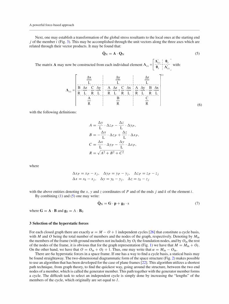
Next, one may establish a transformation of the global stress resultants to the local ones at the starting endj of the member i (Fig. 3). This may be accomplished through the unit vectors along the three axes which arerelated through their vector products. It may be found that:
Q̄N = � · QN (5)
The matrix � may now be constructed from each individual element with:
(6)
with the following definitions:
A = �y
L· �zP − �z
L· �yP ,
B = −�x
L· �zP + �z
L· �xP ,
C = �x
L· �yP − �y
L· �xP ,
R =√
A2 + B2 + C2
where
�xP = xP − x j , �yP = yP − y j , �zP = zP − z j
�x = xk − x j , �y = yk − y j , �z = zk − z j
with the above entities denoting the x, y and z coordinates of P and of the ends j and k of the element i .By combining (1) and (5) one may write:
Q̄N = G · p + g0 · s (7)
where G = � · B and g0 = � · B0
3 Selection of the hyperstatic forces
For each closed graph there are exactly α = M − O + 1 independent cycles [26] that constitute a cycle basis,with M and O being the total number of members and the nodes of the graph, respectively. Denoting by Minthe members of the frame (with ground members not included), by Of the foundation nodes, and by Oin the restof the nodes of the frame, it is obvious that for the graph representation (Fig. 1) we have that M = Min + Of .On the other hand, we have that O = Oin + Of + 1. Thus, one may write that α = Min − Oin.
There are 6α hyperstatic forces in a space frame. If one has a way to find a cycle basis, a statical basis maybe found straightaway. The two-dimensional diagrammatic form of the space structure (Fig. 2) makes possibleto use an algorithm that has been developed for the case of plane frames [22]. This algorithm utilizes a shortestpath technique, from graph theory, to find the quickest way, going around the structure, between the two endnodes of a member, which is called the generator member. This path together with the generator member formsa cycle. The difficult task to select an independent cycle is simply done by increasing the “lengths” of themembers of the cycle, which originally are set equal to 1.

K. V. Spiliopoulos, N. G. Dais
k
m
no
l
q
p
1
1
1
1 1
1
11
k
m
no
l
q
p
1 1
1
1
1
2
2
2
k
m
no
l
q
p
2
22 2
2
2
2
2
(a) (b) (c)
Fig. 5 Mesh base formation
Fc
Mc
j
r
Fig. 6 Hyperstatic pair at each cycle
A cycle will enter the cycle basis if it satisfies the following admissibility rule:
(length of the path) < 2 · [(nodes along the path) − 1
]
If this rule is satisfied, the cycle enters the basis and the lengths of the members of the path become 2.The steps of the algorithm may be seen in Fig. 5, where a subgraph has been extracted from a main graph
(Fig. 5a). Starting from the node k and selecting km as a generator member, the minimum path whose lengthis equal to 2 satisfies the admissibility rule and the cycle klmk enters the basis. The lengths of the membersof the cycle then become equal to 2 (Fig. 5b). This cycle cannot be reselected because it will not pass theadmissibility rule. Next, by picking up, for example kq, as a generator member the next obvious cycle entersthe cycle basis (Fig. 5c).
There are cases of complicated graphs that this simple process may leave out some cycle [22], but thereare remedies to overcome this problem. For such a case, it appears computationally more useful to use analternative equivalent rule (this rule is employed in the present work), that is to add, to the length of the path,the length of the generator member. So the above rule may now be replaced by:
(length of the cycle) < 2 · [(nodes along the path)
]
For the structure of Fig. 1, such a cycle basis may be seen in Fig. 2.Starting with the nodes having the higher valency (number of members incident to a node) guarantees an
almost minimal cycle basis in terms of the number of elements that constitute a cycle.Each of the selected cycles may now be visualized as its real three-dimensional nature. In Fig. 6 one may
see such a cycle. If we make a cut at any such cycle, a pair of resultant forces and moments Fc and Mc thatconstitute the hyperstatic forces for this cycle will appear. This pair may be analyzed in their components alongthe global axes x, y, z. Equilibrium with each of these components leads to stress resultants at each starting endj of the members that are met going around the perimeter of the cycle. More specifically, the opposites of thesehyperstatic components are transferred to produce the corresponding forces and moments at the starting endj of each member of the cycle. The moments have to be augmented by the cross product of the components ofthe distance vector r from the cut to the end j (Fig. 6) with the hyperstatic force vector Fc. So one may write:
F (m)j = −F (m)
c
M (m)j = −M (m)
c − (rj × Fc
)(m) (8)
where m is equal to either x or y or z.

A powerful force-based approach
sF
jr
j
Fig. 7 Equilibrium with external load
(a)
6cQ
cκS c
κψ
4cQ
4κn
6κnκn
cQ
6cQ
4cQ
cQ
(b)
Fig. 8 a Linearized yield surface, b typical yield plane
If we provide unit values for the components of Fc and Mc the equilibrium matrix B may be established.It is obvious that if the specific member happens to be a part of another cycle too, the stress resultants for thismember will be additive.
As far as equilibrium with the external loads is concerned, the shortest path technique is used to find thequickest way of each load to the ground in the form of 3D cantilevers (Fig. 1). Such a typical load path maybe seen in Fig. 7. The forces and moments produced by the load vector components at the starting end j ofeach member along this path may be found in an analogous way as above:
F (m)j = −F (m)
s
M (m)j = − (
rj × Fs)(m) (9)
For unit values for the components of Fs, the entries to the matrix B0 may be found. It is obvious that ifthe specific member happens to be a part of other load paths, its stress resultants will be additive.
4 Problem formulation
We assume a perfectly plastic material. Plasticity is considered concentrated at the critical cross sectionslocated at the member’s end nodes. A “generalized plastic hinge” of zero length will appear whenever thecombination of the components of the vector Q̄c at a cross section c touches the generally nonlinear plasticyield surface. An interaction between two components may be seen in Fig. 8.
The yield surface may then be linearized using planes to approximate it. The plastic strain vector isconsidered orthogonal to any of these planes and directed outward; the length of this vector on any such planeκ is denoted by λ̇κ . Thus, one may write for the plastic vector at a particular critical section c:

K. V. Spiliopoulos, N. G. Dais
˙̄qpl,cκ = λ̇c
κ · nκ , λ̇cκ ≥ 0 (10)
where nκ denotes the outward unit normal vector to the plane κ (Fig. 8b).The sign convention of the components of the plastic vector follows the ones of the corresponding stress
resultants.Plastically admissible combinations of stress resultants are those for which the stress vector Q̄c at a critical
section lies within the yield surface. This may be expressed [27] through:
nTκ · Q̄c + �c
κ = Scκ , �c
κ ≥ 0 (11)
The complementary ways of the activation or not of the κth yield surface are given by the well-knowncomplementarity condition:
�cκ · λ̇c
κ = 0 (12)
If we group the terms nκ , Sκ , λ̇κ in N, S, and λ̇, respectively, for all the possible planes at the critical sectionsof all the members of the frame, Eq. (7) after using the transformation (4), together with Eqs. (11) and (12), arethe Karush–Kuhn–Tucker conditions of the plastic limit analysis [28]. These lead to the following force-basedunsafe program which needs to be solved:
Minimize s = STλ̇Subject to:[
gT0 · T · N
GT · T · N
]λ̇ =
[10
]
λ̇ ≥ 0
(13)
where N =⎡
⎢⎣
N1 . . . 0...
. . ....
0 · · · Nncs
⎤
⎥⎦
with the dimensions being (6 · ncs) × (npl · ncs), where ncs denotes the number of the critical sections of theframe equal to 2 · Min, and npl the number of planes that each yield surface is linearized with; for a properdescription npl ≥ 8.
Any standard LP algorithm, like the simplex technique or an interior-point algorithm [12], may be used tosolve the linear program (13). Interior-point algorithms, which are particularly suited to solve sparse large-scaleproblems with linear or nonlinear constraints (e.g., [17,29]), are increasingly been employed in limit analysisproblems, the last decade. In the present work both sparse solvers, one using the simplex algorithm and oneusing a LP interior-point algorithm, have been implemented. Both solvers are contained in the optimizationpackage MOSEK [30].
5 Computational and programming considerations
Based on the duality of mathematical programming, four different limit analysis LP programs, in the frameworkof either the force or the displacement method, may be written. The variables of these LP programs may beeither kinematic or static ones. Also, the number of constraints of the primal LP is equal to the number ofvariables of the dual LP.
The number of constraints of the kinematic program (13), for a space frame with no releases, is m =1 + 6 · α = 1 + 6 · (Min − Oin), whereas the number of variables, with the variables being the lengths ofthe plastic vectors, is nv = npl · ncs. On the other hand, the kinematic LP program that may be formulatedusing the alternative displacement method has m′ = 1 + 6 · Min constraints and n′
v = npl · ncs + 6 · Oinvariables, with the extra terms being the independent displacements of the frame [27]. The size of the matricesinvolved (i.e., the number of constraints and the number of variables) is of course one parameter that influencesthe computing time. Thus, a force-based LP like the kinematic program (13), which has the fewer number ofconstraints and variables, is the more suitable to solve.
Additionally, the procedure of establishing a near-optimal cycle basis that was described above leads tohypersparse G matrices, which one should take into advantage, using sparse solvers [30].

A powerful force-based approach
7
6
5
4
3
2
1
Fig. 9 Part of a general multistorey–multibay frame
The very sparse form of the equilibrium matrix B may be easily demonstrated in the one-storey configurationof Figs. 1, 2. We may see that there are, at mostly, two nonzero block entries rowise (Eq. 14).
(14)
Q(i)N ,p is the 6 × 1 vector of the independent forces of the member i due to the indeterminacy of the frame, p j
is the 6 × 1 vector of hyperstatic forces of a topological cycle j , and B(i)j is the corresponding 6 × 6 block
entry in the B matrix.On the other hand, the equilibrium, in a displacement-based LP formulation, is expressed by equilibrating
the forces, acting on a node, with the stress resultants of the members that are incident to this node [20]. Builtin this way the equilibrium matrix becomes denser than above. This may be easily seen for the configurationof Fig. 1 where three nonzero 6 × 6 block entries would be needed rowise, since most of the nodes connectthree members.
The same pattern difference between the two formulations holds for the most general case, shown in Fig. 9,where one may see a part of a frame that consists of several bays and storeys. It is easy now to visualize thatas any member will belong to at most four cycles (a typical member with end nodes 1 and 2 is shown in thefigure), the maximum number of entries in the equilibrium matrix for the force-based approach will be fournonzero 6 × 6 block entries rowise. At the same time, we see that the members connected to a typical node(node 1 in the figure) are six, which will require six nonzero block entries rowise if the equilibrium matrixwere to be built in a displacement-based formulation.
Thus, the force-based formulation presented, combined with the solution of the kinematic program, is themost efficient, in terms of computing time, 3D frame limit analysis procedure that may be written.
A computer program that implements the theory described above was written in FORTRAN. The shortestpath technique introduced by Nicholson [31] is used, whose coding may be found in the literature [32]. TheLagrange multipliers of the optimum solution provide values for the hyperstatic forces p from which using(7), a safe distribution of the stress resultants may be established.
K. V. Spiliopoulos, N. G. Dais
(a) (b)
Py
/2
/2
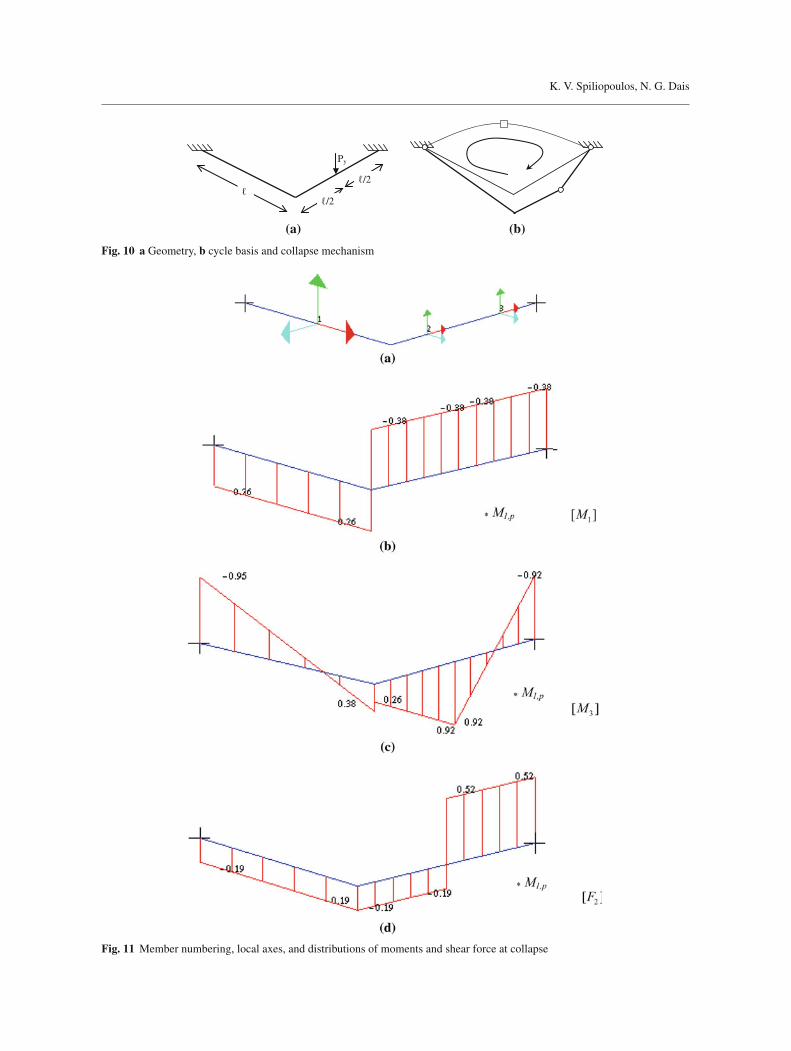
Fig. 10 a Geometry, b cycle basis and collapse mechanism
Fig. 11 Member numbering, local axes, and distributions of moments and shear force at collapse
A powerful force-based approach
Py
Py
Py
Py
Py
Py
Py
Py
Py
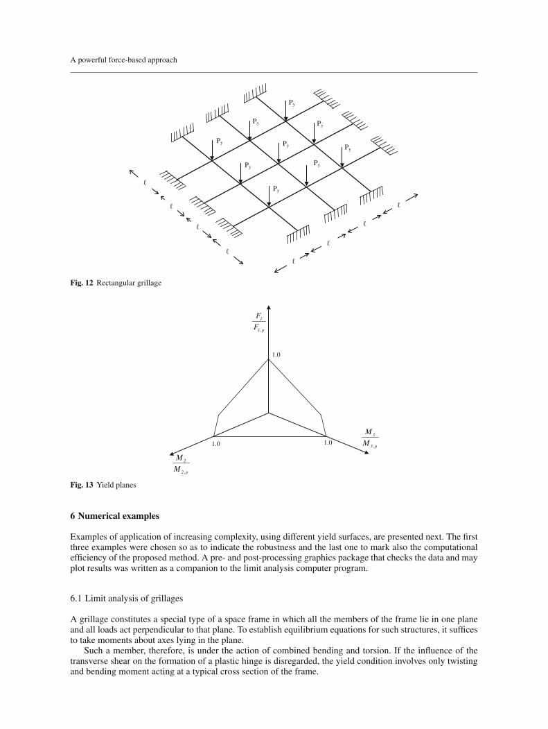
Fig. 12 Rectangular grillage
,
1
1 p
F
F
1.01.0
1.0
,
3
3 p
M
M
,
2
2 p
M
M
Fig. 13 Yield planes
6 Numerical examples
Examples of application of increasing complexity, using different yield surfaces, are presented next. The firstthree examples were chosen so as to indicate the robustness and the last one to mark also the computationalefficiency of the proposed method. A pre- and post-processing graphics package that checks the data and mayplot results was written as a companion to the limit analysis computer program.
6.1 Limit analysis of grillages
A grillage constitutes a special type of a space frame in which all the members of the frame lie in one planeand all loads act perpendicular to that plane. To establish equilibrium equations for such structures, it sufficesto take moments about axes lying in the plane.
Such a member, therefore, is under the action of combined bending and torsion. If the influence of thetransverse shear on the formation of a plastic hinge is disregarded, the yield condition involves only twistingand bending moment acting at a typical cross section of the frame.
K. V. Spiliopoulos, N. G. Dais
7.31
5 m
W12
x87
W 1
2x53
W 1
2x53
W 12x26
W 12x26W 12x26 X
Z
W 12x26
7.315 m7.315 m
(a)
(b)
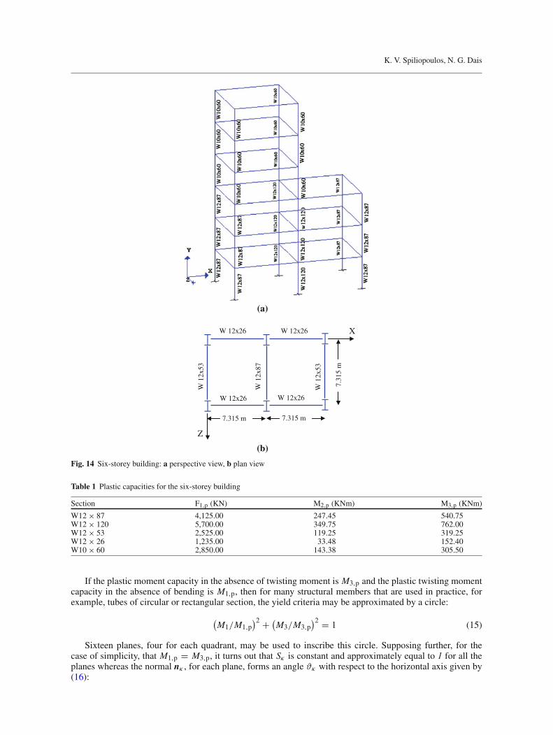
Fig. 14 Six-storey building: a perspective view, b plan view
Table 1 Plastic capacities for the six-storey building
Section F1,p (KN) M2,p (KNm) M3,p (KNm)
W12 × 87 4,125.00 247.45 540.75W12 × 120 5,700.00 349.75 762.00W12 × 53 2,525.00 119.25 319.25W12 × 26 1,235.00 33.48 152.40W10 × 60 2,850.00 143.38 305.50
If the plastic moment capacity in the absence of twisting moment is M3,p and the plastic twisting momentcapacity in the absence of bending is M1,p, then for many structural members that are used in practice, forexample, tubes of circular or rectangular section, the yield criteria may be approximated by a circle:
(M1/M1,p
)2 + (M3/M3,p
)2 = 1 (15)
Sixteen planes, four for each quadrant, may be used to inscribe this circle. Supposing further, for thecase of simplicity, that M1,p = M3,p, it turns out that Sκ is constant and approximately equal to 1 for all theplanes whereas the normal nκ , for each plane, forms an angle ϑκ with respect to the horizontal axis given by(16):

A powerful force-based approach
Fig. 15 a Member numbering and local axes. b Distribution of plastic hinges in collapse mechanism
ϑκ = π
16+ (κ − 1) · π
8, κ=1,2,…,16 (16)
Equation (16) may be used to form the (6 × 16) Nc matrix for each critical cross section c:
Nc =
⎡
⎢⎢⎢⎢⎢⎣
0 0 · · · · · · 00 0 · · · · · · 00 0 · · · · · · 0
cos ϑ1 cos ϑ2 · · · · · · cos ϑ160 0 · · · · · · 0
sin ϑ1 sin ϑ2 · · · · · · sin ϑ16
⎤
⎥⎥⎥⎥⎥⎦
, c = 1, 2, . . . , ncs (17)

K. V. Spiliopoulos, N. G. Dais
Table 2 Safe force and moment distribution for the six-storey building at collapse
Member no. Critical sect. F1 F2 F3 M1 M2 M3
1 1 −586.96 225.02 −22.69 8.38 0 502.282 −586.96 225.02 −22.69 8.38 83.02 −320.86
2 3 35.72 −41.07 0 −45.49 0 −150.24 35.72 −41.07 0 −45.49 0 150.2
3 5 −869.99 314.28 −32.38 −115.58 0 703.856 −869.99 314.28 −32.38 −115.58 118.44 −445.8
4 7 15.86 41.4 0 −337.94 0 151.428 15.86 41.4 0 −337.94 0 −151.42
5 9 −385.42 158.84 55.07 9.38 0 515.4910 −385.42 158.84 55.07 9.38 −201.46 −65.53
6 11 0 87.29 0 251.3 0 319.2512 0 87.29 0 251.3 0 −319.25
7 13 −915.16 62.6 3.6 0 0 473.3814 −915.16 62.6 3.6 0 −13.15 244.4
8 15 0 −41.67 0 −307.74 0 −152.416 0 −41.67 0 −307.74 0 152.4
9 17 −1823.23 150.33 −3.6 294.01 0 583.0518 −1823.23 150.33 −3.6 294.01 13.15 33.15
10 19 11.26 41.48 0 −408.26 0 151.7120 11.26 41.48 0 −408.26 0 −151.71
11 21 −1772.48 189.69 0 0.37 0 346.9422 −1772.48 189.69 0 0.37 0 −346.94
12 23 0 −87.29 0 −146.49 0 −319.2524 0 −87.29 0 −146.49 0 319.25
13 25 0 147.85 0 −65.32 0 540.7526 0 147.85 0 −65.32 0 −540.75
14 27 −456.7 151.64 −58.41 8.38 −213.67 43.8828 −456.7 151.64 −58.41 8.38 0 −510.82
15 29 35.72 −41.07 0 −191.57 0 −150.230 35.72 −41.07 0 −191.57 0 150.2
16 31 −747.34 240.9 −12.53 −115.58 54.35 387.432 −747.34 240.9 −12.53 −115.58 100.17 −493.81
17 33 28.1 41.19 0 −37.13 0 150.6734 28.1 41.19 0 −37.13 0 −150.67
18 35 −254.82 85.45 70.94 9.38 201.26 −84.2336 −254.82 85.45 70.94 9.38 −58.22 −396.81
19 37 0 87.29 0 98.79 0 319.2538 0 87.29 0 98.79 0 −319.25
20 39 −609.72 62.6 3.6 0 −112.06 255.9140 −609.72 62.6 3.6 0 −125.21 26.93
21 41 0 −41.67 0 18.15 0 −152.442 0 −41.67 0 18.15 0 152.4
22 43 −1405.57 150.33 7.67 294.01 79.17 473.3844 −1405.57 150.33 7.67 294.01 51.12 −76.52
23 45 11.26 41.48 0 −369.3 0 151.7146 11.26 41.48 0 −369.3 0 −151.71
24 47 −1467.24 189.69 −11.26 0.37 −5.21 380.5748 −1467.24 189.69 −11.26 0.37 35.99 −313.32
25 49 0 −87.29 0 −87.46 0 −319.2550 0 −87.29 0 −87.46 0 319.25
26 51 0 147.85 0 −118.59 0 540.7552 0 147.85 0 −118.59 0 −540.75
27 53 −326.44 78.26 −94.13 8.38 −237.66 054 −326.44 78.26 −94.13 8.38 106.66 −286.26
28 55 −66.7 −35.33 −1.15 88.58 −8.38 −110.1256 −66.7 −35.33 −1.15 88.58 0 148.28
29 57 −624.49 167.51 −4.91 −115.58 −17.94 −107.4958 −624.49 167.51 −4.91 −115.58 0 −720.26
30 59 −99.03 34.16 −1.28 −156.46 0 146.2960 −99.03 34.16 −1.28 −156.46 9.38 −103.61
31 61 −124.44 12.07 99.03 9.38 191.23 −114.6962 −124.44 12.07 99.03 9.38 −171.03 −158.84
32 63 −62.6 86.2 0 67.42 0 315.2964 −62.6 86.2 0 67.42 0 −315.29

A powerful force-based approach
Table 2 Continued
Member no. Critical sect. F1 F2 F3 M1 M2 M3
33 65 −304.29 62.6 3.6 0 −71.6 364.3366 −304.29 62.6 3.6 0 −84.76 135.35
34 67 −3.6 −41.61 0 −450.64 0 −152.1868 −3.6 −41.61 0 −450.64 0 152.18
35 69 −987.91 150.33 18.93 294.01 170.4 76.7870 −987.91 150.33 18.93 294.01 101.16 −473.12
36 71 −22.53 41.29 0 −243.32 0 151.0172 −22.53 41.29 0 −243.32 0 −151.01
37 73 −1162 189.69 −22.53 0.37 −28.26 375.2374 −1162 189.69 −22.53 0.37 54.14 −318.66
38 75 −58.35 −86.28 0 −96.87 0 −315.5676 −58.35 −86.28 0 −96.87 0 315.56
39 77 0 147.85 0 102.32 0 540.7578 0 147.85 0 102.32 0 −540.75
40 79 −200.92 64.37 −27.43 0 −100.33 −59.2880 −200.92 64.37 −27.43 0 0 −294.73
41 81 −27.43 22.9 −4.02 −193.21 0 150.7182 −27.43 22.9 −4.02 −193.21 29.41 −16.83
42 83 −488.87 94.27 27.43 −115.58 100.33 65.5384 −488.87 94.27 27.43 −115.58 0 −279.3
43 85 0 73.11 −5.29 −2.82 0 319.2586 0 73.11 −5.29 −2.82 38.73 −215.57
44 87 −570 150.33 0 294.01 0 274.9588 −570 150.33 0 294.01 0 −274.95
45 89 0 20.83 −4.58 340.59 −33.48 090 0 20.83 −4.58 340.59 0 −152.4
46 91 −857.95 131.34 0 0.37 0 240.2392 −857.95 131.34 0 0.37 0 −240.23
47 93 −143.61 −84.8 0 −150.71 0 −310.1794 −143.61 −84.8 0 −150.71 0 310.17
48 95 −132.15 138.62 0 0 0 208.6596 −132.15 138.62 0 0 0 −298.42
49 97 0 20.83 −4.58 −81.45 0 152.498 0 20.83 −4.58 −81.45 33.48 0
50 99 −362.6 16.86 −5.29 −144.99 14.02 −153.25100 −362.6 16.86 −5.29 −144.99 33.38 −214.94
51 101 −47.92 4.75 1.78 −33.38 118.12 0102 −47.92 4.75 1.78 −33.38 105.13 −34.78
52 103 −341.24 145.75 5.29 221.81 2.82 281.21104 −341.24 145.75 5.29 221.81 −16.55 −251.95
53 105 0 27.7 −3.07 367.02 −22.44 50.25106 0 27.7 −3.07 367.02 0 −152.4
54 107 −575.84 −7.7 0 0.37 −1.69 −270.64108 −575.84 −7.7 0 0.37 −1.69 −242.49
55 109 0 −87.29 0 −154.09 0 −319.25110 0 −87.29 0 −154.09 0 319.25
56 111 −63.79 69.81 0 0 −1.69 102.28112 −63.79 69.81 0 0 −1.69 −153.08
57 113 0 25.4 −3.57 166.17 0 152.4114 0 25.4 −3.57 166.17 26.14 −33.42
58 115 −170.04 −13.18 −3.52 −60.36 0 −296.39116 −170.04 −13.18 −3.52 −60.36 12.87 −248.16
59 117 −90.14 31.84 3.52 −46.29 86.49 82118 −90.14 31.84 3.52 −46.29 60.76 −150.89
60 119 −187.71 94.77 3.52 94.24 −33.42 149.85120 −187.71 94.77 3.52 94.24 −46.29 −196.81
61 121 0 20.6 −4.63 45.92 −33.48 0122 0 20.6 −4.63 45.92 0.37 −150.71
62 123 −284.37 −4.63 0 0.37 0 −290.26124 −284.37 −4.63 0 0.37 0 −273.33
63 125 0 −87.29 0 −150.71 0 −319.25126 0 −87.29 0 −150.71 0 319.25

K. V. Spiliopoulos, N. G. Dais
6.1.1 Right-angle bent frame
To test the software written, as a first example of application, the unsymmetrical right-angle bent (Fig. 10a) issolved. In Fig. 10b one may see the unique cycle identified by the computer program together with the collapsemechanism. This mechanism is the same over-complete mechanism as it was also pointed out by Heyman[33], who solved this problem analytically. The collapse load factor comes out to be Pc
y = 0.7109M1,p, which
is almost identical to the one analytically computed [33]: Pcy = 16√
10· M1,p
== 0.7155M1,p
In Fig. 11 one may see the evaluated, by the program, distributions of the various stress resultants. To beable to determine also their directions, the local axes of the members are also plotted.
6.1.2 Rectangular grillage
The rectangular grillage shown in Fig. 12 is the next example of grillage type of problems. This example hasbeen analytically solved by Chakrabarty [34]. The computed load factor turns out to be Pc
y = 2.30M1,p/
which compares very well to the analytically evaluated Pcy = 2.33M1,p/.
6.2 Limit analysis of space frames under biaxial bending and axial force
Next, examples concerning 3D steel frames using the AISC [35] interaction surfaces for compact wide-flangesections are examined. For a specific cross section c, these may be expressed through the following equations:
αc1 · |F1| + αc
2 · |M2| + αc3 · |M3| = Sc
0 for |F1|/Fc1,p ≥ 0.2
αc4 · |F1| + αc
5 · |M2| + αc6 · |M3| = Sc
0 for |F1|/Fc1,p < 0.2 (18)
where αc1 = Sc
0Fc
1,p, αc
2 = 8Sc0
9Mc2,p
, αc3 = 8Sc
09Mc
3,p, αc
4 = Sc0
2Fc1,p
, αi5 = Sc
0Mc
2,p, αc
6 = Sc0
Mc3,p
with Fc1,p, Mc
2,p, Mc3,p being the corresponding plastic capacities of the axial force and of the bending
moments of the cross section, respectively, whereas Sc0 is its yield stress.
If one expands (18), we turn up with sixteen equations each one of which corresponds to the equation of aplane. If we plot these equations in a three-dimensional space, with the axes being the normalized axial forceand the normalized bending moments, we can distinguish four quadrants for either a positive or a negativeaxial force. Two planes may be drawn for each quadrant that are represented by either the first or the secondof the equations (18). Two such planes in the first quadrant for positive values of the stress resultants may beseen in Fig. 13.
Assuming Sc0 to be equal to Sc
κ , which is the distance of the origin of the axes (Fig. 8), equation (18)is the Hessian normal form of the equation of a plane and thus the various triads (±)αc
l , l = 1, . . . , 3 or(±)αc
l , l = 4, . . . , 6 play the role of the components of the unit normal vector to the plane κ . Thus, the (6×16)Nc matrix for each cross section c will now look like:
Nc =
⎡
⎢⎢⎢⎢⎢⎣
αc1 αc
1 αc1 −αc
1 −αc1 −αc
1 αc1 −αc
1 αc4 αc
4 αc4 −αc
4 −αc4 −αc
4 αc4 −αc
40 0 0 0 0 0 0 0 0 0 0 0 0 0 0 00 0 0 0 0 0 0 0 0 0 0 0 0 0 0 00 0 0 0 0 0 0 0 0 0 0 0 0 0 0 0
−αc2 αc
2 αc2 αc
2 −αc2 −αc
2 −αc2 αc
2 −αc5 αc
5 αc5 αc
5 −αc5 −αc
5 −αc5 αc
5−αc3
−αc3
αc3
αc3
αc3
−αc3
αc3
−αc3
−αc6 −αc
6 αc6 αc
6 αc6 −αc
6 αc6 −αc
6
⎤
⎥⎥⎥⎥⎥⎦
6.2.1 Six-storey building
The six-storey frame of Fig. 14, which was considered in [15], offers a first example. The yield strength ofall the members is equal to 250 MPa. For the various members of the frame, AISC [35] sections were used,whose plastic capacities may be seen in Table 1.
The structure is subjected to both horizontal and vertical loads that vary proportionally. Wind loads alongthe z direction represent the horizontal loading. These loads were simulated as point loads applied at everybeam to column joint having a value of 26.70 KN.
A powerful force-based approach
(a)
(b)Z
w 1
6x36
w 1
6x36
w 2
1x57
w 12x26
w 12x26
w 1
6x36
w 2
1x57
w 1
6x36
w 12x26
w 12x26w 12x26 X
w 12x26
7.315 m 7.315 m
7.315 m
7.
315
m
7.
315
m
w 12x26
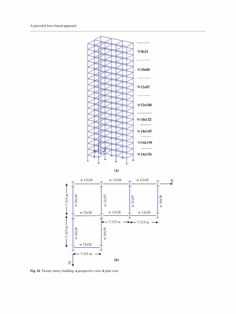
Fig. 16 Twenty-storey building: a perspective view, b plan view
K. V. Spiliopoulos, N. G. Dais
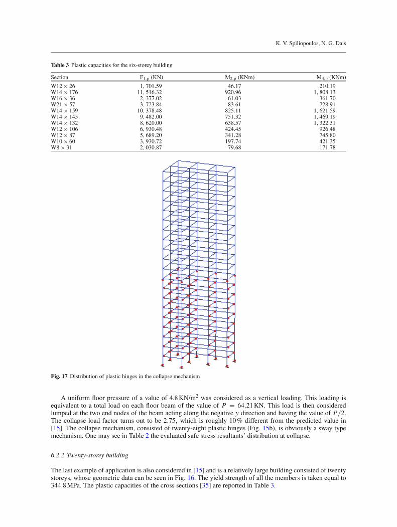
Table 3 Plastic capacities for the six-storey building
Section F1,p (KN) M2,p (KNm) M3,p (KNm)
W12 × 26 1, 701.59 46.17 210.19W14 × 176 11, 516.32 920.96 1, 808.13W16 × 36 2, 377.02 61.03 361.70W21 × 57 3, 723.84 83.61 728.91W14 × 159 10, 378.48 825.11 1, 621.59W14 × 145 9, 482.00 751.32 1, 469.19W14 × 132 8, 620.00 638.57 1, 322.31W12 × 106 6, 930.48 424.45 926.48W12 × 87 5, 689.20 341.28 745.80W10 × 60 3, 930.72 197.74 421.35W8 × 31 2, 030.87 79.68 171.78
Fig. 17 Distribution of plastic hinges in the collapse mechanism
A uniform floor pressure of a value of 4.8 KN/m2 was considered as a vertical loading. This loading isequivalent to a total load on each floor beam of the value of P = 64.21 KN. This load is then consideredlumped at the two end nodes of the beam acting along the negative y direction and having the value of P/2.The collapse load factor turns out to be 2.75, which is roughly 10 % different from the predicted value in[15]. The collapse mechanism, consisted of twenty-eight plastic hinges (Fig. 15b), is obviously a sway typemechanism. One may see in Table 2 the evaluated safe stress resultants’ distribution at collapse.
6.2.2 Twenty-storey building
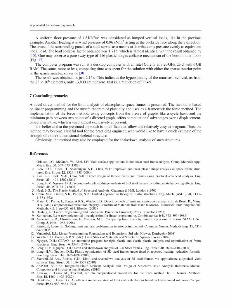
The last example of application is also considered in [15] and is a relatively large building consisted of twentystoreys, whose geometric data can be seen in Fig. 16. The yield strength of all the members is taken equal to344.8 MPa. The plastic capacities of the cross sections [35] are reported in Table 3.
A powerful force-based approach
A uniform floor pressure of 4.8 KN/m2 was considered as lumped vertical loads, like in the previousexample. Another loading was wind pressure of 0.96 kN/m2 acting at the backside face along the z direction.The areas of the surrounding panels of a node served as a means to distribute this pressure evenly as equivalentnodal load. The load collapse factor obtained was 1.715, which is almost identical with the result obtained by[15]. One may observe a pure sway type of 116 plastic hinges collapse mechanism of the bottom nine floors(Fig. 17).
The computer program was run at a desktop computer with an Intel Core i7 at 3.20 GHz CPU with 6 GBRAM. The same, more or less, computing time was spent for the solution with either the sparse interior pointor the sparse simplex solver of [30].
The result was obtained in just 2.15 s. This indicates the hypersparcity of the matrices involved, as fromthe 23 × 106 elements, only 13,800 are nonzero, that is, a reduction of 99.4 %.
7 Concluding remarks
A novel direct method for the limit analysis of elastoplastic space frames is presented. The method is basedon linear programming and the unsafe theorem of plasticity and uses as a framework the force method. Theimplementation of the force method, using concepts from the theory of graphs like a cycle basis and theminimum path between two points of a directed graph, offers computational advantages over a displacement-based alternative, which is used almost exclusively at present.
It is believed that the presented approach is not difficult to follow and relatively easy to program. Thus, themethod may become a useful tool for the practicing engineer, who would like to have a quick estimate of thestrength of a three-dimensional skeletal structure.
Obviously, the method may also be employed for the shakedown analysis of such structures.
References
1. Orbison, J.G., McGuire, W., Abel, J.F.: Yield surface applications in nonlinear steel frame analysis. Comp. Methods Appl.Mech. Eng. 33, 557–573 (1982)
2. Liew, J.Y.R., Chen, H., Shanmugan, N.E., Chen, W.F.: Improved nonlinear plastic hinge analysis of space frame struc-tures. Eng. Struct. 22, 1324–1338 (2000)
3. Kim, S-E., Park, M-H., Choi, S-H.: Direct design of three-dimensional frames using practical advanced analysis. Eng.Struct. 23, 1491–1502 (2001)
4. Long, H.V., Nguyen, D.H.: Second-order plastic-hinge analysis of 3-D steel frames including strain hardening effects. Eng.Struct. 30, 3505–3512 (2008)
5. Neal, B.G.: The Plastic Method of Structural Analysis. Chapman & Hall, London (1970)6. Cohn, M.Z., Ghosh, S.K., Parimi, S.R.: Unified approach to theory of plastic structures. Eng. Mech. (ASCE) 98, 1133–
1158 (1972)7. Maier, G., Pastor, J., Ponter, A.R.S., Weichert, D.: Direct methods of limit and shakedown analysis. In: de Borst, R., Mang,
H.A. (eds.) Comprehensive Structural Integrity—Fracture of Materials from Nano to Macro, : Numerical and ComputationalMethods, vol. 3, pp 637–684. Elsevier (2003)
8. Dantzig, G.: Linear Programming and Extensions. Princeton University Press, Princeton (1963)9. Karmarkar, N.: A new polynomial time algorithm for linear programming. Combinatorica 4(4), 373–395 (1984)
10. Andersen, K.D., Christiansen, E., Overton, M.L.: Computing limit loads by minimizing a sum of norms. SIAM J. Sci.Comp. 3, 1046–1062 (1998)
11. Pastor, F., Loute, E.: Solving limit analysis problems: an interior point method. Commun. Numer. Methods Eng. 21, 631–642 (2005)
12. Vanderbei, R.J.: Linear Programming: Foundations and Extensions. 3rd edn. Kluwer, Dordrecht (2008)13. Weichert, D., Ponter, A.R.S. (eds.): Limit States of Materials and Structures. Springer, Wien (2009)14. Nguyen, D.H.: CEPAO—an automatic program for rigid-plastic and elastic-plastic analysis and optimization of frame
structures. Eng. Struct. 6, 33–51 (1984)15. Long, H.V., Nguyen, D.H.: Limit and shakedown analysis of 3-D Steel frames. Eng. Struct. 30, 1895–2004 (2007)16. Long, H.V., Nguyen, D.H.: Plastic optimization of 3D steel frames under fixed or repeated loading: reduction formula-
tion. Eng. Struct. 32, 1092–1099 (2010)17. Skordeli, M-AA., Bisbos, C.D.: Limit and shakedown analysis of 3d steel frames via approximate ellipsoidal yield
surfaces. Eng. Struct. 32, 1556–1557 (2010)18. SAP2000 V-14.2.4. Integrated Finite Element Analysis and Design of Structures-Basic Analysis Reference Manual.
Computers and Structures Inc, Berkeley (2010)19. Kaneko, I., Lawo, M., Thierauf, G.: On computational procedures for the force method. Int. J. Numer. Methods.
Eng. 18, 1469–1495 (1982)20. Damkilde, L., Høyer, O.: An efficient implementation of limit state calculations based on lower-bound solutions. Comput.
Struct 49(6), 953–962 (1993)

K. V. Spiliopoulos, N. G. Dais
21. Kaveh, A., Koohestani, K.: An efficient graph-theoretical force method for three-dimensional finite element analysis.Commun. Numer. Methods Eng. 24, 1533–1551 (2008)
22. Spiliopoulos, K.V.: On the automation of the force method in the optimal plastic design of frames. Comp. Methods Appl.Mech. Eng. 141, 141–156 (1997)
23. Spiliopoulos, K.V.: A fully automatic force method for the optimal shakedown design of frames. Comp. Mech. 23(4), 299–307 (1999)
24. Spiliopoulos, K.V., Patsios, T.N.: A quick estimate of the strength of uniaxially tied framed structures. J. Constr. SteelRes. 65, 1763–1775 (2009)
25. de Henderson, J.C., Maunder, E.A.W.: A problem in applied topology: on the selection of cycles for the flexibility analysisof skeletal structures. J. Inst. Maths. Appl. 5, 254–269 (1969)
26. de Henderson, J.C., Bickley, W.G.: Statical indeterminacy of a structure. J. Aircr Eng. 27, 400–402 (1955)27. Smith, D.L.: Plastic limit analysis. In: Smith DL (ed.) Mathematical Programming Methods in Structural Plasticity.
pp. 61–82, Springer, Berlin (1990)28. Maier, G.: Linear flow-laws of elastoplasticity: a unified general approach. Rendic. Acad. Naz. Lincei, Series 8, 47, 266 (1969)29. Trillat, M., Pastor, J.: Limit analysis and Gurson’s model. Eur. J. Mech. Solids 24, 800–819 (2005)30. MOSEK ApS, Denmark.: the MOSEK optimization tools version 6.0 (revision 135)—user’s manual and reference (2012)
Download at http://www.mosek.com31. Nicholson, T.A.J.: Finding the shortest route between two points in a network. Comput. J. 26, 275–280 (1966)32. Lau, H.T.: Algorithms on Graphs. Tab Books (1989)33. Heyman, J.: Elements of the Theory of Structures. Cambridge University Press, Cambridge (1996)34. Chakrabarty, J.: Theory of Plasticity. Elsevier Butterworth-Heinemann, Oxford (2006)35. AISC.: Load and Resistance Factor Design Specification for Steel Buildings. American Institute of Steel Construction,
Chicago (1993)