ORIGINAL Species-occupancy distribution removes …lifeserv.bgu.ac.il/wb/yziv/media/Gavish_and_Ziv-2016-Journal_of... · Species-occupancy distribution removes an excessive parameter

ORIGINALARTICLE

Species-occupancy distribution removesan excessive parameter from species-area relationshipYoni Gavish* and Yaron Ziv

Spatial Ecology Laboratory, Department of

Life Sciences, Ben-Gurion University of the

Negev, Beer-Sheva 84105, Israel

*Correspondence and Current Address: Yoni

Gavish, School of Biology, University of Leeds,

Leeds LS2 9JT, United Kingdom. E-mail:

[email protected]

ABSTRACT

Aim Although species-occupancy distributions (SODs) and species-area rela-

tionships (SARs) arise from the two marginal sums of the same presence/ab-

sence matrices, the two biodiversity patterns are usually explored

independently. Here, we aim to unify the two patterns for isolate-based data

by constraining the SAR to conserve information from the SOD.

Location Widespread.

Methods Focusing on the power-model SAR, we first developed a constrained

form that conserved the total number of occupancies from the SOD. Next, we

developed an additive-constrained SAR that conserves the entire shape of the

SOD within the power-model SAR function, using a single parameter (the

slope of the endemics-area relationship). We then relate this additive-con-

strained SAR to multiple-sites similarity measures, based on a probabilistic

view of Sørensen similarity. We extend the constrained and additive-con-

strained SAR framework to 23 published SAR functions. We compare the fit of

the original and constrained forms of 12 SAR functions using 154 published

data sets, covering various spatial scales, taxa and systems.

Main conclusions In all 23 SAR functions, the constrained form had one

parameter less than the original form. In all 154 data sets the model with the

highest weight based on the corrected Akaike’s information criteria (wAICc)

had a constrained form. The constrained form received higher wAICc than the

original form in 98.79% of valid pairwise cases, approaching the wAICc

expected under identical log-likelihood. Our work suggests, both theoretically

and empirically, that all SAR functions may have one unnecessary parameter,

which can be excluded from the function without reduction in goodness-of-fit.

The more parsimonious constrained forms are also easier to interpret as they

reflect the probability of a randomly chosen occupancy to be found in an iso-

late. The additive-constrained SARs accounts for two complimentary turn-over

components of occupancies: turnover between species and turnover between

sites.

Keywords

biodiversity patterns, islands, Jaccard, landscape, macroecology, multiple-sites

similarity, occupancy-frequency distribution, patches, Sørensen, spatial

ecology

INTRODUCTION

Studying biodiversity distribution patterns characterizes a

major exploration line in contemporary ecology due to both

basic and applied needs. This exploration requires

biodiversity data collection of diverse species located at dif-

ferent spatial extents. Consequently, most biodiversity studies

end up with a species-by-site table filled with presence/ab-

sence data (hereafter we refer to a presence of a species in a

site as occupancy). Summing this community matrix for

ª 2016 John Wiley & Sons Ltd http://wileyonlinelibrary.com/journal/jbi 1doi:10.1111/jbi.12869

Journal of Biogeography (J. Biogeogr.) (2016)

each site over all species yields the total number of species

sampled within each site (Fig. 1A). Similarly, when summed

for each species over all sites, the marginal sums yield the

number of sites in which a species occurred (i.e. the species-

occupancy level). These two sets of marginal sums give rise

to two important biodiversity patterns – the species-occu-

pancy distribution (SOD, the number of species that

occurred in each occupancy level, for example, McGeoch &

Gaston, 2002; Jenkins, 2011) and the species–area relation-

ship (SAR, the change in species richness with a change in

area).

SARs and SODs can be constructed from data collected in

various ways, including nested quadrats, quadrats in a con-

tiguous grid, quadrats in a non-contiguous grid, and non-

overlapping areas of various sizes (types I–IV sensu Scheiner,

2003 respectively). Here, we focus on type IV SARs, and fol-

lowing Tjørve & Turner (2009), we refer to the sites as iso-

lates (non-overlapping sites with biologically or

environmentally defined borders that differ from one another

in various attributes such as area, shape, heterogeneity and

spatial context). Most SOD studies focused on contiguous or

non-contiguous equal-sized quadrat (type II or III), in which

SOD shape is highly dependent upon the choice of grain

size, while type IV SOD, on which we focus here, has the

advantage of working on naturally occurring grains: the iso-

lates. Despite numerous studies of SARs in island-like sys-

tems, we are not aware of any manuscript that focused on

type IV SODs.

Indeed, among the two biodiversity patterns, SARs have

received the most attention, with at least 23 mathematical

functions suggested to describe the pattern (Tjørve, 2003,

2009; Williams et al., 2009). In fact, SARs are one of the

most fundamental patterns of ecology. Empirically, SARs

have been explored in numerous study systems, covering a

wide range of scales, focusing on diverse taxa, and using var-

ious methods (Rosenzweig, 1995; Scheiner, 2003; Drakare

et al., 2006; Triantis et al., 2012). SARs exhibit a consistent

pattern: the number of species increases with area, thus con-

sidered as a general law of ecology (Rosenzweig, 1995). SARs

have also been the subject of extensive theoretical research,

either aiming to explain their properties or as a starting rule

from which other patterns emerge (e.g. Rosenzweig & Ziv,

1999). The generality and centrality of SARs triggered their

usage in applied ecology. Among others, SARs are used to

(A)

(B)

(C)

(D)(E)

(F)

Figure 1 General framework for species-occupancy distributions (SODs) and species–area relationships (SARs). The marginal sums ofpresence/absence tables (A) yields the number of species per isolate which can be used to plot the general SAR (D). The second

marginal sums yields the number of isolates per species (i.e. the species-occupancy level), which can be used to produce the SOD (C).However, the presence/absence table can be rearranged by grouping species from the same occupancy level (B). From the resulting

N 9 N square matrix the occupancy-specific SARs can be produced (E) as well as a weighted version of the SOD (wSOD, C). Theadditive-constrained SAR develop here is based on this square matrix. The notations used here and in text are given in (F).

Journal of Biogeographyª 2016 John Wiley & Sons Ltd

2

Y. Gavish and Y. Ziv

estimate extinction debts (Brooks et al., 2002; Kuussaari

et al., 2009), identify biodiversity hotspots (Myers et al.,

2000; Gavish, 2011), and optimize reserve design (Bascompte

et al., 2007; Tjørve, 2010; Gavish et al., 2012).

In contrast, SODs remained relatively unexplored, perhaps

due to the complexity of shapes they can take. Unlike SARs,

which are usually described by convex functions with no

asymptote (Triantis et al., 2012), SODs may be unimodal,

bimodal, random or uniform, and their modes may occur

for satellite (rare), central or core (common) species

(McGeoch & Gaston, 2002; Jenkins, 2011; Hui, 2012). Fur-

thermore, bimodal SODs may be symmetrical or asymmetri-

cal, and if asymmetric they may have a stronger or weaker

mode for rare or common species. Until recently, only one

method (Tokeshi, 1992), based on comparison of the size of

the satellite and core modes to an expected null model, was

used to describe SOD’s shape. Recently, Jenkins (2011) intro-

duced the ranked species-occupancy curves (rSOC) as an

alternative method and Hui (2012) clarified the direct link

between the two patterns. Similar to species-abundance dis-

tribution and ranked abundance curves, SOD and rSOC are

two alternative ways to present the same information.

Although SODs and SARs arise from the two marginal

sums of the same presence/absence table, the two patterns

were rarely explored simultaneously (but see: Hui &

McGeoch, 2014; Pan, 2015). In fact, in most cases they were

explored simultaneously only when both were derived from

species-abundance data, either through null models (Cole-

man, 1981), neutral models (Hubbell, 2001) or metapopula-

tion-based models (Ovaskainen & Hanski, 2003). The aim of

this paper is to develop the direct link between SODs and

SARs for island-like systems within a single framework.

Within this framework, the shape of the SOD itself can be

explored in relation to species traits, thereby providing a

more mechanistic understating of the SAR. Furthermore,

mechanistic SAR hypotheses such as the transient hypothesis

(MacArthur & Wilson, 1967), rescue effects (Brown & Kod-

ric-Brown, 1977), target area effects (Gilpin & Diamond,

1976) and small island effects (Lomolino, 2000), are medi-

ated through changes in species-occupancy levels.

MATERIAL AND METHODS

Mathematical developments

We develop the direct link between SOD and SAR by con-

straining the SAR to conserve the data encompassed by the

SOD. Starting with the power-model (Arrhenius, 1921), we

first developed the constrained-SAR model, by forcing the

SAR to conserve the observed total number of occupancies

(thereby cancelling-out one of the power-model parameters).

Then, in the additive-constrained SAR model, we fit a sepa-

rate constrained-SAR model to the species of each occupancy

level, and then sum the results over all the occupancy levels.

By describing the change in SAR parameters with occupancy

level we provide a novel one-parameter SAR function that

predicts not only the shape of the global SAR, but also the

SAR of each occupancy level, while conserving the entire

shape of the SOD. The parameter of this additive model is

the slope of the endemics-area relationship. Subsequently, we

relate the SOD to multiple-sites similarity indices and gener-

alize to 23 known SAR functions.

The power-model SAR

We start with a presence/absence matrix of M species in N

isolates (Fig. 1A, see notations in Fig. 1F). Each species is

notated with m (in the range {1,2,. . .,M}), each isolate with

i {1,2,. . .N} and each entry as Oi,m (that can take the value

of 1 or 0). The observed number of species in isolate i (here-

after, Si) is the sum of Oi,m over all M species, and if Ai is

the area of isolate i, the global SAR can be constructed

(Fig. 1D). The occupancy level of species m (hereafter, jm) is

the sum of Oi,m over all N isolate (thus jm is in the range

{1,2,. . .,N}). The SOD explores how the number of species

in occupancy level j (hereafter Rj) changes with j (Fig. 1C).

Thus, summing Rj over all the occupancy levels (all j in the

range {1,2,. . .,N}) yields M. The presence/absence matrix

cab be restructured as a square N 9 N matrix, with the

number of presences from each occupancy level that were

found in each isolate (hereafter Si,j, Fig. 1B). The total num-

ber of occupancies can be estimated in three ways: by sum-

ming Oi,m over all the M species, by summing Si over all the

N isolates, and by summing j�Rj over all the occupancy

levels.

Given the observed Si and Ai, the original power-model

SAR (Arrhenius, 1921) takes the form:

EðSiÞorig: ¼ c � Azi (1)

With E(Si)orig. as the number of species predicted for isolate

i by the power-model and c and z as scaling parameters. The

total number of occupancies predicted by the power-model

is the sum of equation 1 over all n isolates. To constrain the

power-model SAR such that it will conserve the observed

total number of occupancies, we set Σj(j�Rj) = Σic�Aiz and

multiply equation 1 by Σj(j�Rj)/Σic�Aiz:

EðSiÞcons: ¼ c � Azi �

PNj¼1ðj � RjÞPNi¼1ðc � Pz

i Þ¼XN

j¼1ðj � RjÞ � Az

iPni¼1 A

zi

(2)

with E(Si,j)cons. being the expected number of species in iso-

late i according to the constrained power-model. Adding the

total number of occurrences constraint to the power-model

SAR eliminates parameter c, which allows the predicted sum

of occupancies to differ from the observed one, leaving only

parameter z. Furthermore, Aiz/ΣiAiz is the probability of a

single occupancy to be found in isolate i. Although this con-

strain can be employed with no knowledge of the SOD, we

base it on the SOD’s arguments to exemplify the effect of

focusing only on species from a single occupancy level. In

fact, when equation 2 is fitted only to the subset of species

from occupancy level j (Fig. 1E), we get:


3

SOD removes excessive SAR parameter

EðSi;jÞcons: ¼ ðj � RjÞ � AzjiPn

i¼1 Azji

(3)

with E(Si,j)cons. being the expected number of species from

occupancy level j in isolate i, and zj the slope of the SAR of

occupancy level j. If we assume that the SAR of all occu-

pancy levels can be described by a power-model (see below)

then equation 3 can be summed to produce a second

approximation of the global SAR:

EðSiÞadd:cons: ¼XN

j¼1j � Rj

� � � AzjiPn

i¼1 Azji

" #(4)

with E(Si)add.cons. being the expected number of species in

isolate i according to the additive-constrained power-model.

We are not aware of any publication that explores the

change of zj with j, which we term ‘z-occupancy curves’.

However, endemics-area relationships (the SAR when includ-

ing only species that are endemic to a single isolate, i.e.

j = 1) usually have relatively high zj values (Rosenzweig,

1995; Triantis et al., 2008). Eventually, zj values for j = N

are, by definition, zero (the species occur on all isolates,

Fig. 1E). In addition, equations 2 and 3 can estimate the

maximal value of z that will ensure that none of the isolates

contains more species than the actual size of the species pool

(ΣjRj), or the number of species in occupancy level j (Rj),

denoted as zmax and zj,max respectively. When setting the

monotonically increasing (for z > 0) equations 2 and 3 to

equal ΣjRj or Rj (respectively) and solving for the largest iso-

late (here, isolate i = N) we get:

Azmax

NPNi¼1 A

zmax

i

¼PN

j¼1 RjPNj¼1ðj � RjÞ

(5)

Azj;max

NPNi¼1 A

zj;max

i

¼ Rj

ðj � RjÞ ¼1

j(6)

This means that zmax is the value of z for which the proba-

bility of randomly drawn occupancy to be in the largest iso-

late equals the inverse of the mean occupancy level.

Although zj is unbounded for j = 1, zj of all other occupancy

levels have a maximal value (zj,max) that is independent of

the number of species and depends mainly on the area distri-

bution (Ai values, equation 6). The maximal values result in

a decreasing function when plotting zj,max against j. There-

fore, we expect zj to decrease with j in a predictable manner,

according to a function F(zj|j) that intersects the abscissa at

j = n. Consequently, we get:


j¼1ðj � RjÞ � A

Fðzj jjÞiPN

i¼1 AFðzj jjÞi

" #(7)

Although various functions may describe the shape of

the z-occupancy curve, we focused here on the form given

in equation 8, and when plugging it into equation 7 we

get:

FðzjjjÞ : Zj ¼ a � ð1� logNjÞ (8)


j¼1ðj � RjÞ � A

a�ð1�logN jÞiPN

i¼1 Aa�ð1�logN jÞi

" #(9)

We chose equation 8 for three main reasons. First, it is an

exponential decay function zj = a � b�ln(j) that intersects

the point (N,0) (such that b = a/ln(N)), and thus always

predict zj values of 0 when j = N. Second, preliminary analy-

sis of several data sets revealed it to be a good candidate

model. Third, its only parameter (a) is biologically meaning-

ful- it is the z value of the endemic-area relationship. In fact,

equation 9 is a SAR function that incorporates the entire

observed shape of the SOD into the SAR, provides predic-

tions for the overall SAR, as well as for the SAR of each

occupancy level and has a single, ecologically meaningful

parameter (a). Other F(zj|j) functions with more complex

shapes or with better theoretical grounds can be developed,

perhaps after more detailed exploration of the shape of z-

occupancy curves is carried.

Finally, if the constrained and additive-constrained

model provides comparable predictions, and equations 2

and 9 are divided by the total number of occupancies, we

get:

SiPNj¼1½ðj � RjÞ�

¼ AziPn

i¼1 Azi

ffiXN

j¼1

j � RjPNj¼1½ðj � RjÞ�

!� A

a�ð1�logN jÞiPN

i¼1 Aa�ð1�logN jÞi

!" #

(10)

so that the probability of a randomly chosen occupancy to

be found in isolate i is similar (up to the error associated

with the models) to the sum over all the occupancy levels of

the multiplication of two probabilities. The first is the proba-

bility of a randomly chosen occupancy to be from occupancy

level j. The second is the conditional probability of this occu-

pancy to be found in isolate i, given the SAR of occupancy

level j. The two probabilities reflect the two marginal sums

of the presence/absence data table. In fact, the first probabil-

ity is the generalization of Sørensen probabilities to multiple-

sites, as explained in the next section.

Similarity indices, SODs and weighted SODs

The most commonly used pairwise similarity indices of bin-

ary data are Jaccard and Sørensen. Let S1 and S2 be the num-

ber of species in isolates 1 and 2, respectively, and let Ssharedbe the number of species shared by the two isolates. Jaccard

similarity can be expressed as Sshared/(S1 + S2 � Sshared),

while Sørensen similarity index is 2�Sshared/(S1 + S2) (Chao

et al., 2005). Therefore, Jaccard similarity is the ratio of the

number of species in occupancy level j = 2 and the total

number of species. Sørensen similarity index is the ratio of

the number of occupancies in occupancy level j = 2 and the

total number of occupancies. When viewed as probabilities,

Jaccard is the probability of randomly selecting a species that


4


is shared by the two isolates. Sørensen is the probability of

randomly selecting an occupancy from a species shared by

two isolates. That is, when n = 2, Jaccard can be expressed

as R2/(R1 + R2), while Sørensen can be expressed as 2�R2/

(1�R1 + 2�R2). Jaccard and Sørensen dissimilarities are the

complimentary of the indices to 1, which can be expressed as

R1/(R1 + R2) and 1�R1/(1�R1 + 2�R2) respectively. Thus, when

there are only two isolates, the additive-constrained SAR

(equation 10) explicitly contains Sørensen similarity and dis-

similarity index as weights.

The SOD summarizes the change in Rj with j. If we stan-

dardize the SOD by dividing it by ΣjRj, we get for each occu-

pancy level the term Rj/ΣjRj, which is the generalization of

Jaccard probabilities into multiple isolates. A weighted form

of the SOD (wSOD, Fig. 1C) summarizes the change in j�Rj

with j. When standardizing the wSOD by dividing it with

Σj(j�Rj), we get for each occupancy level the term j�Rj/Σj(j�Rj),

which is the generalization of Sørensen probabilities to mul-

tiple isolates. Since the basic unit of type IV SARs is occu-

pancy and not species, Sørensen probabilities are more

relevant to the study of type IV SARs. Therefore, when there

are more than two sites, equation 10 incorporates the gener-

alization of Sørensen probabilities into the general SAR

framework.

We suggest that summary statistics of the standardized

SOD and wSOD can be considered as measures of beta

diversity, as their constituting values may serve as the build-

ing blocks for multiple-sites similarity indices. Such multi-

ple-sites similarity measures may differ from one another in

their treatment of the difference between species in occu-

pancy level. For example, the strictest definition of Jaccard

multiple-sites similarity may be the proportion of species

that are found in all isolates from the total number of spe-

cies, that is, Rn/ΣjRj, and for Sørensen, the equivalent pro-

portion of occupancies from the total number of

occupancies, that is, n�Rn/Σj(j�Rj). The least strict may be the

proportion of species/occupancies that are found in at least

two isolates, that is, Σj6¼1[Rj/ΣjRj] for Jaccard, and Σj 6¼1[j�Rj/Σjj�Rj] for Sørensen. In fact, if wj is the weight given to occu-

pancy level j in the multiple-sites similarity measure (such

that 0 ≤ wj ≤ 1), then a general multiple-sites similarity of

Jaccard and Sørensen, which still conserves the 2 isolates

interpretation as the proportion of species or occupancies

may be:

Jacmult ¼PN

j¼1½wj � Rj�PNj¼1½Rj�

(11)

S�rmult ¼PN

j¼1½wj � j � Rj�PNj¼1½j � Rj�

(12)

with w1 = w2 = . . . = wN�1 = 0 and wN = 1 for the most

strict example while w1 = 0 and w2 = w3 = . . . = wN = 1 for

the least strict example. A more interesting option for the

weights may be the proportion of isolates pairs in which a

species co-occur, resulting with

Jacmult ¼XN

j¼1

jðj� 1ÞNðN � 1Þ �

RjPNj¼1½Rj�

" #(13)

S�rmult ¼Xn

j¼1

jðj� 1ÞNðN � 1Þ �

j � RjPNj¼1½j � Rj�

" #(14)

which converges to Jaccard and Sørensen similarity indices

for n = 2, while satisfying w1 = 0 and wN = 1 and keeping

the original probabilistic interpretation of the indices. We

note though, that the multiple-sites similarity indices them-

selves are not incorporated directly into the SAR, but rather

they are built by the same building blocks as the SAR. We

further note that published multiple-sites versions of Jaccard

(Baselga, 2012) and Sørensen similarity indices (Baselga,

2010) can also be restructured using terms from the SOD as:

Jacmult;Bas ¼PN

j¼1ðj � RjÞ �PN

j¼1 Rj

h iPN

j¼1ðj � RjÞ �PN

j¼1 Rj

h iþPN

j¼1 Rj � j � ðN � jÞ� �¼

PNj1 ½ðj� 1Þ � Rj�PN

j1 ½ðj� 1þ jðN � jÞÞ � Rj�ð15Þ

S�rmult;Bas ¼2 � PN

j¼1ðj �RjÞ�PN

j¼1 Rj

h i2 � PN

j¼1ðj �RjÞ�PN

j¼1Rj

h iþPN

j¼1 Rj � j � ðN � jÞ� �¼

PNj1 ½ð2j� 2Þ �Rj�PN

j1 ½ð2j� 2þ jðN � jÞÞ �Rj�ð16Þ

yet, such extensions to multiple-sites do not conserve the

total number of species or occupancies in the denominator,

and therefore loses the probabilistic interpretation of Jaccard

and Sørensen similarity indices. Furthermore, although the

contribution to the similarity measure increases with occu-

pancy level in the numerators of Jacmult,Bas and Sørmult,Bas,

the denominator reaches a maximum value for j = (N + 1)/2

and j = (N + 2)/2 respectively. If the SOD is indeed the uni-

fying concept between beta-diversity and SARs, we suggest

focusing on multiple-sites similarity indices that conserve

the probabilistic interpretation of the SOD and the wSOD.

In addition to the ecological meaning of the probabilities,

it opens a possible direction to incorporate the effect of

unsampled species to multiple-site similarity indices and

SARs, as shown for pairwise similarity by Chao et al. (2005).

Other SAR functions

Constrained SARs and additively constrained SARs can be

based on any SAR function (Tjørve, 2003, 2009; Williams

et al., 2009; Triantis et al., 2012). Repeating the steps that

led from equation 1 to equation 2 for other SAR functions

has a similar effect – all SAR functions lose one of their

parameters (Table 1). Similar additive forms to those shown

here for the power-model can be developed for all other SAR

functions. Therefore, all SAR functions may have one unnec-

essary parameter that can be excluded, apparently, without

loss of statistical power.


5


Empirical analysis of 154 data sets

We explored 154 published data sets (see Appendix S2) to

examine whether a parameter can be dropped without loss

of goodness-of-fit if the SAR is constrained. The data sets

cover various spatial scales (from 6 m2 isolates to inter-pro-

vincial SARs), taxa (fungi, plants, invertebrates and verte-

brates) and systems (inter-provincials, ecoregions, true

islands, fragmented terrestrial landscapes, etc.). Before fitting

any model and to ease the search for appropriate starting

values for parameters, we first standardized the area units to

relative area: Pi = Ai/ΣiAi (and Σi Pi = 1). We fitted each

data set with the original and constrained forms of the

twelve functions given in bold face in Table 1, a total of 24

functions. Non-linear least square regressions (using the

Levenberg-Marquardt convergence algorithm) were used to

Table 1 The original and constrained forms of 23 known species–area relationship (SAR) functions (c, z, f and k are function

parameters). The parameters column indicate the change in the number of parameters when moving from the original to theconstrained form. Functions given in bold face were used in the empirical analysis of the 154 data sets.

Name Original form (Si=) Constrained form (Si=) Parameters

Lin. c + z � Ai

Pjðj � RjÞ � ð1þz0 �AiÞ

Ri ½1þz0 �Ai � 2 ? 1 (z0 = z/c)

Pow. c � Azi

Pjðj � RjÞ � Az

i

Ri ½Azi � 2 ? 1

Pow.Ros. f þ c � Azi

Pjðj � RjÞ � ð1þc0 �Az

iÞ

Ri ½1þc0 �Azi� 3 ? 2 (c0 = c/f)

Ext.P1 c � Az�A�f

i

i

Pjðj � RjÞ � A

z�A�fi

i

Ri Az�Ai�f

i

h i 3 ? 2

Ext.P2 c � Az�f =Ai

i

Pjðj � RjÞ � A

z�f =Aii

Ri Az�f =Aii

� � 3 ? 2

P1 c � Azi � expð�f � AiÞ


i�expð�f �AiÞ

Ri ½Azi�expð�f �AiÞ� 3 ? 2

P2 c � Azi � expð�f =AiÞ


i �ð1�expð�f =AiÞÞRi ½Az

i �ð1�expð�f =AiÞÞ� 3 ? 2

Exp. c þ z � logðAiÞP

jðj � RjÞ � ð1þz0 �logðAiÞÞRi ½1þz0 �logðAiÞ� 2 ? 1 (z0 = z/c)

Kob. c � logð1þ Ai=zÞP

jðj � RjÞ � log�ð1þAi=zÞRi ½log�ð1þAi=zÞ� 2 ? 1

Mon. c=ð1þ z=AiÞP

jðj � RjÞ � ð1=ð1þz=AiÞÞRi ½1=ð1þz=AiÞ� 2 ? 1

MMF c=ð1þ f � A�zi Þ P

jðj � RjÞ � ð1=ð1þf �A�zi ÞÞ

Ri ½1=ð1þf �Azi Þ� 3 ? 2

Arc.Log. c=ðf þ A�zi Þ P

jðj � RjÞ � ð1=ðfþA�zi ÞÞ

Ri ½1=ðfþA�zi Þ� 3 ? 2

Neg.Exp. c � ð1� expð�z � AiÞÞP

jðj � RjÞ � ð1�expð�z�AiÞÞRi ½1�expð�z�AiÞ� 2 ? 1

Chp.Ric. c � ð1� expð�z � AiÞÞfP

jðj � RjÞ � ð1�expð�z�AiÞÞfRi ½1�expð�z�AiÞ�f 3 ? 2

Wei.3 c � 1� expð�z � Afi Þ

� � Pjðj � RjÞ � ð1�expð�z�Af

iÞÞ

Ri ½1�expð�z�Af

iÞ� 3 ? 2

Wei.4 c � 1� exp �z � Afi

� �� k Pjðj � RjÞ � ð1�expð�z�Af

iÞÞk

Ri ½1�expð�z�Af

iÞ�k 4 ? 3

Asy. f � c � z�AiP

jðj � RjÞ � ð1þc0 �z�Ai ÞRi ½1þc0 �z�Ai � 3 ? 2 (c0 = c/f)

Rat. c þ z � Aið Þ= 1þ f � Aið Þ Pjðj � RjÞ � ð1þz0 �AiÞ=ð1þf �AiÞ

Ri ½ð1þz0 �AiÞ=ð1þf �AiÞ� 3 ? 2 (z0 = z/c)

Gom. c � exp �exp �z Ai � fð Þð Þð Þ Pjðj � RjÞ � expð�expð�z�ðAi�f ÞÞÞ

Ri ½expð�expð�z�ðAi�f ÞÞÞ� 3 ? 2

Beta.P c � 1� 1þ Ai=zð Þf� ��k

� Pjðj � RjÞ � 1� 1þðAi=zÞfð Þ�k

� �Ri e 1� 1þðAi=zÞfð Þ�k� �� 4 ? 3

Com.Log. c= 1þ exp �z � Ai þ fð Þð Þ Pjðj � RjÞ � 1= 1þexpð�z�Aiþf Þð Þð Þ

Ri 1= 1þexpð�z�Aiþf Þð Þð Þ½ � 3 ? 2

EVF. c � 1� exp � exp z � Ai þ fð Þð Þð Þ Pjðj � RjÞ � 1�exp �expðz�Aiþf Þð Þð Þ

Ri 1�exp �expðz�Aiþf Þð Þð Þ½ � 3 ? 2

Lom. c= 1þ zlog f =Aið Þ� �� Pjðj � RjÞ � 1= 1þ zlogðf =Ai Þð Þð Þð Þ

Ri 1= 1þ zlogðf =Ai Þð Þð Þð Þ 3 ? 2

Pow. – Power; Pow.Ros. – Power Rosenzweig; Ext.P1– Extended Power 1; Ext.P2– Extended Power 2; P1 – Persistence Function 1; P2 – Persis-

tence Function 2; Exp. – Exponential; Kob. – Kobayashi Logarithmic; Mon. – Monod; MMF. – Morgan-Mercer-Flodin; Arc.Log. – Archibald

Logistic; Neg.Exp. – Negative Exponential; Chp.Ric. – Chapman-Richards; Wei.3 – Weibull-3; Wei.4 – Weibull-4; Asy. – Asymptotic; Rat. –Rational. Gom. – Gompertz; Beta.P. – Beta-P; Com.Log. – Common Logistic; EVF. – Extreme-Value Function; Lom. – Lomolino function.


6


fit each data set with the 24 models, and various parameter-

starting values were used to avoid local minima. After con-

vergence, for the original and constrained forms of each SAR

function, the estimated parameters of the form that resulted

with lower residuals sum-of-squares (RSS) were used as the

starting parameters of the second form in an additional non-

linear regression and the newly estimated parameters were

kept if the fit was improved.

After fitting the 24 models, we calculated for each model

the corrected Akaike’s information criteria (AICc; Burnham

& Anderson, 2002; see Appendix S1 in Supporting Informa-

tion). Next, AICc weights (wAICcg, with g being the name of

the model out of G models) were calculated for the entire

set of 24 models (i.e. G = 24). We then focused on each of

the 12 SAR functions separately and estimated the wAICcg of

the functions’ original and constrained forms of each SAR

function (i.e. 12 different sets, each with G = 2). For the 12

sets, we estimated the expected wAICc for the special case in

which the original and constrained form have identical log–likelihood and only differ in the number of parameters

(Appendix S1). Finally, we applied a least-square linear

regression of the observed wAICc of the constrained form

against the expected value under identical log-likelihood and

explored whether the confidence intervals of the intercept

and slope overlapped with zero and one respectively.

The 154 data sets were also used to explore the shape of

z-occupancy curves. Firstly, for each data set, we fitted equa-

tion 3 separately for the species from each occupancy level.

This yielded the observed zj values for every j for which some

species were observed. Next, we fitted the observed z-occu-

pancy curve with equation 8, while recording the explained

variance and significance. For the data sets presented in

Fig. 3, we fitted equation 9 as well, and compared the pre-

dicted z-occupancy curve to the fitted one. We further com-

pared the AICc values and weights of the original power-

model (equation 1), constrained power-model (equation 2)

and additive-constrained power-model (equation 9).

Finally, for the 154 data sets we estimated the Sørensen

multiple-sites similarity index based on equation 14. We

used linear regression to explore the relation between the

power-model z values and the multiple-sites similarity value.

For this analysis, we use only data set where the power-

model explained variance was larger than 0.25. All regression

analyses were carried out with the minpack.lm package in R

(R Development Core Team, 2014).

RESULTS

When comparing the 24 models, in all 154 data sets the

model with the highest wAICc had a constrained form. In

general, SAR functions with the highest wAICc usually had

only two parameters in the original form (80% of data sets),

had a convex shape (63%) and had no asymptote (64%).

Indeed, in 32% of the data sets, the best SAR function had

all three of these characters. The power-model had the high-

est wAICc for 25.4% of the data sets.

From a total of 1848 (12 9 154) combinations of SAR

models and data sets, the non-linear regression achieved con-

vergence for both the original and constrained forms in 1811

analyses. The constrained form received a higher wAICc than

the original form in 1789 out of 1811 pairwise comparisons

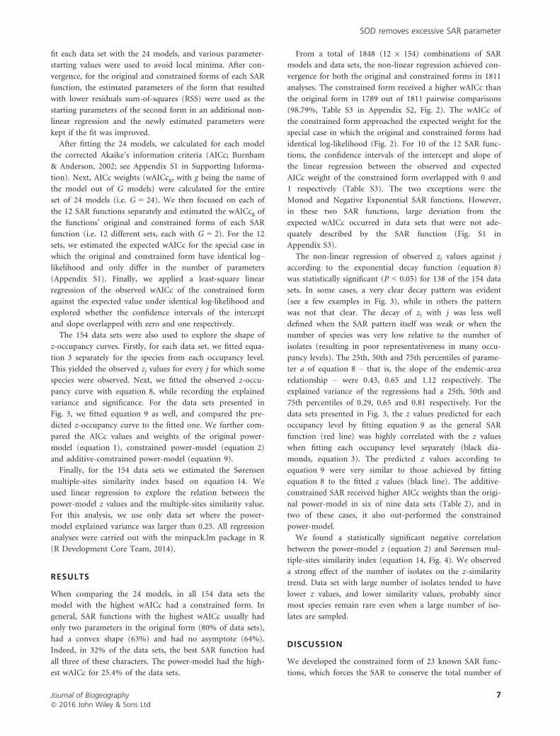
(98.79%, Table S3 in Appendix S2, Fig. 2). The wAICc of

the constrained form approached the expected weight for the

special case in which the original and constrained forms had

identical log-likelihood (Fig. 2). For 10 of the 12 SAR func-

tions, the confidence intervals of the intercept and slope of

the linear regression between the observed and expected

AICc weight of the constrained form overlapped with 0 and

1 respectively (Table S3). The two exceptions were the

Monod and Negative Exponential SAR functions. However,

in these two SAR functions, large deviation from the

expected wAICc occurred in data sets that were not ade-

quately described by the SAR function (Fig. S1 in

Appendix S3).

The non-linear regression of observed zj values against j

according to the exponential decay function (equation 8)

was statistically significant (P < 0.05) for 138 of the 154 data

sets. In some cases, a very clear decay pattern was evident

(see a few examples in Fig. 3), while in others the pattern

was not that clear. The decay of zj with j was less well

defined when the SAR pattern itself was weak or when the

number of species was very low relative to the number of

isolates (resulting in poor representativeness in many occu-

pancy levels). The 25th, 50th and 75th percentiles of parame-

ter a of equation 8 – that is, the slope of the endemic-area

relationship – were 0.43, 0.65 and 1.12 respectively. The

explained variance of the regressions had a 25th, 50th and

75th percentiles of 0.29, 0.65 and 0.81 respectively. For the

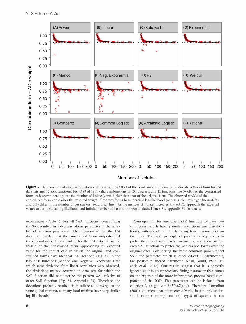
data sets presented in Fig. 3, the z values predicted for each

occupancy level by fitting equation 9 as the general SAR

function (red line) was highly correlated with the z values

when fitting each occupancy level separately (black dia-

monds, equation 3). The predicted z values according to

equation 9 were very similar to those achieved by fitting

equation 8 to the fitted z values (black line). The additive-

constrained SAR received higher AICc weights than the origi-

nal power-model in six of nine data sets (Table 2), and in

two of these cases, it also out-performed the constrained

power-model.

We found a statistically significant negative correlation

between the power-model z (equation 2) and Sørensen mul-

tiple-sites similarity index (equation 14, Fig. 4). We observed

a strong effect of the number of isolates on the z-similarity

trend. Data set with large number of isolates tended to have

lower z values, and lower similarity values, probably since

most species remain rare even when a large number of iso-

lates are sampled.

DISCUSSION

We developed the constrained form of 23 known SAR func-

tions, which forces the SAR to conserve the total number of


7


occupancies (Table 1). For all SAR functions, constraining

the SAR resulted in a decrease of one parameter in the num-

ber of function parameters. The meta-analysis of the 154

data sets revealed that the constrained forms outperformed

the original ones. This is evident for the 154 data sets in the

wAICc of the constrained form approaching its expected

value for the special case in which the original and con-

strained forms have identical log-likelihood (Fig. 3). In the

two SAR functions (Monod and Negative Exponential) for

which some deviation from linear correlation were observed,

the deviations mainly occurred in data sets for which the

SAR function did not describe the pattern well, relative to

other SAR function (Fig. S1, Appendix S3). Therefore, the

deviations probably resulted from failure to converge to the

same global minima, as many local minima have very similar

log-likelihoods.

Consequently, for any given SAR function we have two

competing models having similar predictions and log-likeli-

hoods, with one of the models having fewer parameters than

the other. The basic principle of parsimony requires us to

prefer the model with fewer parameters, and therefore for

each SAR function to prefer the constrained forms over the

original ones. Considering the most common power-model

SAR, the parameter which is cancelled-out is parameter c,

the ‘politically ignored’ parameter (sensu, Gould, 1979; Tri-

antis et al., 2012). Our results suggest that it is correctly

ignored as it is an unnecessary fitting parameter that comes

on the expense of the more informative, process-based com-

ponent of the SOD. This parameter can be isolated from

equation 2, to get: c = Σj(j�Rj)/Σi(Aiz). Therefore, Lomolino

(2000) statement that parameter c ‘varies in a poorly under-

stood manner among taxa and types of systems’ is not

0.00

0.25

0.50

0.75

1.00

0.00

0.25

0.50

0.75

1.00

0.00

0.25

0.50

0.75

1.00

0 50 100 150 200 0 50 100 150 200 0 50 100 150 200 0 50 100 150 200

Number of isolates

Con

stra

ined

form

− A

ICc

wei

ght

(A) Power (B) Linear (C) Kobayashi (D) Exponential

(E) Monod (F)Neg. Exponential (G) P2 (H) Weibull

(I) Gompertz (J)Common Logistic (K) Archibald Logistic (L) Rational

Figure 2 The corrected Akaike’s information criteria weight (wAICc) of the constrained species–area relationships (SAR) form for 154data sets and 12 SAR functions. For 1789 of 1811 valid combinations of 154 data sets and 12 functions, the (wAICc of the constrained

form (red, shown here against the number of isolates), was higher than that of the original form. The observed wAICc of theconstrained form approaches the expected weight, if the two forms have identical log-likelihood (and as such similar goodness-of-fit)

and only differ in the number of parameters (solid black line). As the number of isolates increases, the wAICc approach the expectedvalues under identical log-likelihood and infinite number of isolates (horizontal dashed line). See appendix S1 for details.


8


Z va

lue

Fragmented - Anthropogeic Fragmented - Natural

(A) DS 49

0.0

0.2

0.4

0.6

0.8

1 3 6 9 12 15 18

(B) DS 104

0.0

0.3

0.6

0.9

1.2

1.5

1 2 4 6 8 10

(C) DS 125

0.0

0.2

0.4

0.6

1 3 6 9 12

Archipelagos

(D) DS 16

0.0

0.2

0.4

0.6

1 4 8 12 16 20

(E) DS 38

0.0

0.2

0.4

0.6

0.8

1 2 3 4 5 6 7

(F) DS 64

0.0

0.1

0.2

0.3

0.4

0.5

0.6

0.7

1 3 6 9 12 15 18 21

Archipelagos Ecoregions

(G) DS 115

0.0

0.2

0.4

0.6

0.8

1.0

1 6 12 18 24 30 36 42

(H) DS 136

0.0

0.2

0.4

0.6

0.8

1.0

1 2 3 4 5 6 7 8 9

(I) DS 117

0.0

0.2

0.4

0.6

0.8

1.0

1 15 30 45 60 75 90

Occupancy level

0.8

Figure 3 A few examples of z-occupancy curves. The predicted z values in each occupancy level as predicted when fitting equation 9(red line), compared to the z value obtained when fitting each occupancy level separately with a constrained power-model (equation 3,

black diamonds). The dashed black line was obtained by fitting equation 8 to the fitted z values. Each panel is for one data set (DS),numbered according to Table S2 (Appendix S2).

Table 2 Corrected Akaike’s information criteria (AICc) values and weights of the original power-model (equation 1), the constrained

power-model (equation 2) and the additive-constrained power-model (equation 9) for the nine data sets presented in figure 2. Valuesin parentheses are the ranking of each model according to the AICc weights.

AICc AICc weights

Data set Equation 1 Equation 2 Equation 9 Equation 1 Equation 2 Equation 9

DS49 135.89 133.01 135.90 0.161 (2) 0.679 (1) 0.160 (3)

DS104 50.04 45.79 53.27 0.104 (2) 0.875 (1) 0.021 (3)

DS125 107.16 103.49 106.00 0.111 (3) 0.692 (1) 0.197 (2)

DS16 208.25 205.47 207.81 0.160 (3) 0.642 (1) 0.199 (2)

DS38 108.49 101.49 101.26 0.014 (3) 0.465 (2) 0.521 (1)

DS64 114.13 111.39 113.72 0.162 (3) 0.639 (1) 0.199 (2)

DS115 232.96 230.64 236.1 0.227 (2) 0.725 (1) 0.047 (3)

DS136 58.69 53.91 51.19 0.018 (3) 0.201 (2) 0.781 (1)

DS117 1135.18 1133.04 1133.90 0.172 (3) 0.501 (1) 0.326 (2)


9


surprising, given that even when the area units are standard-

ized, it is a function of the total number of occupancies, the

number of isolates, the distribution of area between isolates

and the second parameter z. Parameter c (and its above

approximation) is usually interpreted as the number of spe-

cies in one unit of area. The general SAR is then constructed

by multiplying the number of species in one unit area by an

area dependent function. This is still true for the constrained

SAR (equation 2). However, we show here that it is also true

for the constrained SAR of all other SAR models (Table 1).

Removing a parameter from a widely used function may

seem to present a small technical improvement. However,

given its broad use and the importance of SARs for various

applications, simplification of SAR models is crucial to

understanding patterns and processes, since simpler models

are easier to interpret. Although having more parameters

allows better fit to data, parameters should be added if the

additional goodness-of-fit is needed to better understand the

pattern. For SARs, this does not seem to be the case. In fact,

the proximity of the wAICc to the expected AICc weight

under identical log-likelihood (Fig. 2) suggests that the two

forms have very similar goodness-of-fit.

By constraining the SAR, we have shown that SAR repre-

sents the turnover of occupancies between isolates. Although

SARs predict the number of species in each isolate, it is more

correct to treat occupancy as their basic unit. To claim that

the unit of SARs is species is similar to claiming that the

unit of the abundance-area relationship (i.e. the total num-

ber of individuals per isolate) is species and not individuals.

Accepting that SARs represent the turnover of occupancies

between isolates suggests that SARs may also be affected by

the second occupancies turnover component – that is, the

turnover of occupancies between species. This second com-

ponent is captured by the SOD and the additive-constrained

SAR.

The additive-constrained SAR (equations 7 and 9) sums

over all the occupancy levels the multiplication of two prob-

abilities. The first is the probability that a random occupancy

is from occupancy level j, and the second is the probability

of this occupancy being in isolate i, given its occupancy level.

The two probabilities represent the two turnover compo-

nents of occupancies: (i) turnover of occupancies between

species, and (ii) turnover of occupancies between isolates.

The first turnover component relates to the shape of the

wSOD, and as such to the extended Sørensen probabilities.

The effect of this turnover component on the SAR’s shape is

evident in the relation between z and the multiple-sites simi-

larity index (Fig. 4). The second relates to the shape of the

z-occupancy curves.

Here we explored a very specific additive-constrained SAR

that assumes a power-model at all occupancy levels. Of

course, similar to the general SAR, this might not be correct

in all data sets. However, even under this strict assumption,

the additive-constrained SAR outperformed the original

power-model in six of nine data sets (Table 2), while provid-

ing excellent prediction to the actual shape of the z-occu-

pancy curves (Fig. 3). Furthermore, even within a given data

set, different models may best describe SARs of different

occupancy levels. Unfortunately, occupancy-specific SARs

have never been explored before, with the exception of the

endemics-area relationship that was mainly explored using a

power-model (Triantis et al., 2008). We predict that the best

fitting SAR model will change in a consistent manner with

occupancy level (e.g. from a sigmoid curve, to power-law

and then to linear models as occupancy increases). Alterna-

tively, additive-constrained SARs can be based on single

models with greater flexibility such as the two models sug-

gested by Tjørve (2012).

The constrained form does not suggest any clear ecological

interpretation of z, yet it is still unclear if any such interpre-

tation will ever arise (Connor & McCoy, 2001; but see:

Rosindell & Cornell, 2007; O’Dwyer & Green, 2010; Grilli

et al., 2012). Mathematically, z is a scaling parameter that

changes the proportion Aiz/Σi(Ai

z), relative to z = 1, for

which each isolate receives a proportion from the total occu-

pancies that is identical to its relative area. Therefore, the

ecological interpretation added in the constrained form is

not in the meaning of z, but rather in the meaning of the

proportion Aiz/Σi(Ai

z). As equation 2 is structured as the

total number of occupancies multiplied by this proportion

we can interpret it as the probability of a randomly drawn

occupancy to be from isolate i. The proportion also explains

why z has maximal values (equation 5), as no isolate can

receive more occupancies than the number of species. This

restriction on the values of z may be the reason why various

theories, in spite of their very different underlying assump-

tions, also predict it to have a restricted range (e.g. Preston,

1962). Note, that zmax cannot be estimated from the original

form of SAR, since many different combinations of c and z

may satisfy the maximal proportion criteria. Similar maximal

values for parameters can be found for six other SAR

0.0

0.2

0.4

0.6

0.8

0.0 0.2 0.4 0.6

Multiple site Sørensen (eq. 14)

Z va

lues

163664100144

Figure 4 The relation between z and Sørensen multiple-sitessimilarity index. The power-model’s z values decrease with

increase in multiple-sites similarity index (y = 0.53 � 0.61 9 x,F113,1 = 14.491, P < 0.001). The size of the points is relative to

the square root of the number of isolates in the data set.


10


functions that have a single parameter in their constrained

form (Table 1).

In a wider perspective, we used the SOD as a pre-defined

pattern that is plugged into the SAR. However, species-occu-

pancy levels may be explored in relation to any of the species

traits. For example, species dispersal ability is likely to affect

the intensity of rescue effects and recolonization rates. Thus,

species with higher dispersal abilities are likely to be found in

more isolates than species with lower dispersal ability. Alterna-

tively, species with high competitive ability are likely to persist

longer in isolates once they are colonized. Thus, species with

high competitive abilities are also lankly to occur on more iso-

lates than species with poor competitive abilities. Now, if we

can model the probability of a species to have a certain occu-

pancy level (j) based on its’ dispersal and competitive abilities,

we can sum these probabilities over all species for a given j to

represent Rj. These Rj can then be used in equations 2, 4 or 9

above. In such analyses, the parameters linking species-occu-

pancy levels to species dispersal and competitive abilities (or

any other relevant trait) can be estimated simultaneously with

the parameters of the SAR, thereby allowing a more mechanis-

tic understanding of SARs. The incorporation of species traits

directly into SAR functions may compliment other relations

between SARs and traits, such as exploring SAR’s slope for var-

ious trait values (Franzen et al., 2012), substituting species

richness with functional trait diversity as the dependent vari-

able (Whittaker et al., 2014) or building SARs from species-

specific incidence functions (Ovaskainen & Hanski, 2003). The

advantage here is that one does not need to know in advance

the effect of these traits on the probability to occur on j iso-

lates, and can learn on it from the SAR function.

Similarly, SARs are only one of the biodiversity patterns

that relate the number of species per isolate with one of the

isolate’s attributes. Other attributes may include, for exam-

ple, habitat heterogeneity, degree of isolation or the availabil-

ity of resources (e.g. species energy relationship). Probably,

many of the mathematical functions used to describe SARs

(Table 1) may be used to describe other biodiversity pat-

terns, such as species-connectivity relationships and species-

heterogeneity relationships. The constrained and additive-

constrained forms may be used to explore any of these biodi-

versity patterns.

Here we show, both theoretically (Table 1) and empirically

(Fig. 2), that all known SAR functions have one unnecessary

parameter. Simplification of models is crucial to understand-

ing patterns and processes, because simpler models are easier

to interpret. By constraining the SAR, we have clarified its

basic units, united all functions to a similar general structure

(Table 1), introduced Sørensen probabilities into the SAR

framework and linked the two sides of presence/absence

tables (Fig. 1). SARs are fundamental to the development

and testing of many ecological theories (McGill, 2010) and

play an important role in conservation and management,

including identifying biodiversity hotspots (Guilhaumon

et al., 2008) and predicting the effect of habitat loss on spe-

cies richness (Rosenzweig et al., 2012; Keil et al., 2015).

Hopefully, our work will shed new light on this important

biodiversity pattern.

ACKNOWLEDGEMENTS

We thank Itamar Giladi and Dror Kapota for important

remarks and suggestions. Burt Kotler, Zvika Abramsky, Ofer

Ovadia, Bob Holt and Bill Kunin provided invaluable com-

ments on earlier versions of this manuscript. Special thanks

to Arnost L. Sizling for his extremely constructive review,

and to two additional anonymous referees and the editor,

Franc�ois Guilhaumon for their comments. YZ was supported

by the Israel Science Foundation (grant 751/09).

REFERENCES

Arrhenius, O. (1921) Species and area. Journal of Ecology, 9,

95–99.Bascompte, J., Luque, B., Olarrea, J. & Lacasa, L. (2007) A

probabilistic model of reserve design. Journal of Theoretical

Biology, 247, 205–211.Baselga, A. (2010) Partitioning the turnover and nestedness

components of beta diversity. Global Ecology and Biogeog-

raphy, 19, 134–143.Baselga, A. (2012) The relationship between species replace-

ment, dissimilarity derived from nestedness, and nested-

ness. Global Ecology and Biogeography, 21, 1223–1232.Brooks, T.M., Mittermeier, R.A., Mittermeier, C.G., da Fon-

seca, G.A.B., Rylands, A.B., Konstant, W.R., Flick, P., Pil-

grim, J., Oldfield, S., Magin, G. & Hilton-Taylor, C.

(2002) Habitat loss and extinction in the hotspots of bio-

diversity. Conservation Biology, 16, 909–923.Brown, J.H. & Kodric-Brown, A. (1977) turnover rates in

insular biogeography – effect of immigration and extinc-

tion. Ecology, 58, 445–449.Burnham, K.P. & Anderson, R. (2002) Model selection and

multimodel inference – a practical information – theoretic

approach, 2nd edn. Springer Press, New-York, USA.

Chao, A., Chazdon, R.L., Colwell, R.K. & Shen, T.J. (2005) A

new statistical approach for assessing similarity of species

composition with incidence and abundance data. Ecology

Letters, 8, 148–159.Coleman, B.D. (1981) On random placement and species-

area relations. Mathematical Biosciences, 54, 191–215.Connor, E.F. & McCoy, E.D. (2001) Species-area relation-

ships. Encyclopedia of biodiversity (ed. by S.A. Levin), pp.

397–411. Academic Press, London, UK.

Drakare, S., Lennon, J.J. & Hillebrand, H. (2006) The imprint

of the geographical, evolutionary and ecological context on

species–area relationships. Ecology Letters, 9, 215–227.Franzen, M., Schweiger, O. & Betzholtz, P.E. (2012) Species-

area relationships are controlled by species traits. PLoS

ONE, 7, 1–10Gavish, Y. (2011) Questioning israel’s great biodiversity –relative to whom? A comment on Roll et al. 2009. Israel

Journal of Ecology & Evolution, 57, 183–192.


11


Gavish, Y., Ziv, Y. & Rosenzweig, M.L. (2012) Decoupling

fragmentation from habitat loss for spiders in patchy agri-

cultural landscapes. Conservation Biology, 26, 150–159.Gilpin, M.E. & Diamond, J.M. (1976) Calcualtion of immi-

gration and extinction curves from species-area-distance

relation. Proceedings of the National Academy of Sciences

USA, 73, 4130–4134.Gould, S.J. (1979) An allometric interpretation of species-

area curves: the meaning of the coefficient. American Nat-

uralist, 114, 335–343.Grilli, J., Azaele, S., Banavar, J.R. & Maritan, A. (2012) Spa-

tial aggregation and the species-area relationship across

scales. Journal of Theoretical Biology, 313, 87–97.Guilhaumon, F., Gimenez, O., Gaston, K.J. & Mouillot, D.

(2008) Taxonomic and regional uncertainty in species-area

relationships and the identification of richness hotspots.

Proceedings of the National Academy of Sciences of the Uni-

ted States of America, 105, 15458–15463.Hubbell, S.P. (2001) The unified neutral theory of biodiversity

and biogeography. Princeton University Press, New-Jersey,

USA.

Hui, C. (2012) Scale effect and bimodality in the frequency

distribution of species occupancy. Community Ecology, 13,

30–35.Hui, C. & McGeoch, M.A. (2014) Zeta diversity as a concept

and metric that unifies incidence-based biodiversity pat-

terns. American Naturalist, 184, 684–694.Jenkins, D.G. (2011) Ranked species occupancy curves reveal

common patterns among diverse metacommunities. Global

Ecology and Biogeography, 20, 486–497.Keil, P., Storch, D. & Jetz, W. (2015) On the decline of biodi-

versity due to area loss. Nature Communications, 6, 1–11.Kuussaari, M., Bommarco, R., Heikkinen, R.K., Helm, A.,

Krauss, J., Lindborg, R., Ockinger, E., Partel, M., Pino, J.,

Roda, F., Stefanescu, C., Teder, T., Zobel, M. & Steffan-

Dewenter, I. (2009) Extinction debt: a challenge for biodiver-

sity conservation. Trends in Ecology & Evolution, 24, 564–571.Lomolino, M.V. (2000) Ecology’s most general, yet protean

pattern: the species-area relationship. Journal of Biogeogra-

phy, 27, 17–26.MacArthur, R.H. & Wilson, E.O. (1967) The theory of island

biogeography. Princeton University Press, New-Jersey, USA.

McGeoch, M.A. & Gaston, K.J. (2002) Occupancy frequency

distributions: patterns, artefacts and mechanisms. Biologi-

cal Reviews, 77, 311–331.McGill, B.J. (2010) Towards a unification of unified theories

of biodiversity. Ecology Letters, 13, 627–642.Myers, N., Mittermeier, R.A., Mittermeier, C.G., da Fonseca,

G.A.B. & Kent, J. (2000) Biodiversity hotspots for conser-

vation priorities. Nature, 403, 853–858.O’Dwyer, J.P. & Green, J.L. (2010) Field theory for biogeog-

raphy: a spatially explicit model for predicting patterns of

biodiversity. Ecology Letters, 13, 87–95.Ovaskainen, O. & Hanski, I. (2003) The species-area rela-

tionship derived from species-specific incidence functions.

Ecology Letters, 6, 903–909.

Pan, X. (2015) Reconstruct species-area theory using set the-

ory. National Academy Science Letters, 38, 173–177.Preston, F.W. (1962) The Canonical distribution of com-

monness and rarity: Part I. Ecology, 13, 182–215.R Development Core Team (2014) R: A Language and Envi-

ronment for Statistical Computing. R Foundation for Sta-

tistical Computing, Vienna, Austria. http://www.R-

project.org.

Rosenzweig, M.L. (1995) Species diversity in space and time.

Cambridge University Press, Cambridge.

Rosenzweig, M.L. & Ziv, Y. (1999) The echo pattern of species

diversity: pattern and processes. Ecography, 22, 614–628.Rosenzweig, M.L., Drumlevitch, F., Borgmann, K.L., Flesch,

A.D., Grajeda, S.M., Johnson, G., Mackay, K., Nicholson,

K.L., Patterson, V., Pri-Tal, B.M., Ramos-Lara, N. & Ser-

rano, K.P. (2012) An ecological telescope to view future

terrestrial vertebrate diversity. Evolutionary Ecology

Research, 14, 247–268.Rosindell, J. & Cornell, S.J. (2007) Species-area relationships

from a spatially explicit neutral model in an infinite land-

scape. Ecology Letters, 10, 586–595.Scheiner, S.M. (2003) Six types of species-area curves. Global

Ecology and Biogeography, 12, 441–447.Tjørve, E. (2003) Shapes and functions of species-area

curves: a review of possible models. Journal of Biogeogra-

phy, 30, 827–835.Tjørve, E. (2009) Shapes and functions of species-area curves

(II): a review of new models and parameterizations. Jour-

nal of Biogeography, 36, 1435–1445.Tjørve, E. (2010) How to resolve the SLOSS debate: lessons

from species-diversity models. Journal of Theoretical Biol-

ogy, 264, 604–612.Tjørve, E. (2012) Arrhenius and Gleason revisited: new

hybrid models resolve an old controversy. Journal of Bio-

geography, 39, 629–639.Tjørve, E. & Turner, W.R. (2009) The importance of samples and

isolates for species-area relationships. Ecography, 32, 391–400.Tokeshi, M. (1992) Dynamics of distribution in animal com-

munities – theory and analysis. Researches on Population

Ecology, 34, 249–273.Triantis, K.A., Mylonas, M. & Whittaker, R.J. (2008) Evolu-

tionary species-area curves as revealed by single-island

endemics: insights for the inter-provincial species-area

relationship. Ecography, 31, 401–407.Triantis, K.A., Guilhaumon, F. & Whittaker, R.J. (2012) The

island species-area relationship: biology and statistics. Jour-

nal of Biogeography, 39, 215–231.Whittaker, R.J., Rigal, F., Borges, P.A.V., Cardoso, P., Ter-

zopoulou, S., Casanoves, F., Pla, L., Guilhaumon, F., Ladle,

R.J. & Triantis, K.A. (2014) Functional biogeography of

oceanic islands and the scaling of functional diversity in

the Azores. Proceedings of the National Academy of Sciences

of the United States of America, 111, 13709–13714.Williams, M.R., Lamont, B.B. & Henstridge, J.D. (2009) Spe-

cies-area functions revisited. Journal of Biogeography, 36,

1994–2004.


12


http://www.R-project.org

http://www.R-project.org

SUPPORTING INFORMATION

Additional Supporting Information may be found in the

online version of this article:

Appendix S1 AICc, wAICc and expected AICc.

Appendix S2 References and information on data sets.

Appendix S3 Linear regressions of wAICc.

BIOSKETCH

Yoni Gavish – Is currently a research fellow at the Univer-

sity of Leeds, working on the development of biodiversity

analysis tools under the EU-BON project. He is interested in

species-distribution models, biodiversity-patterns, commu-

nity modelling and habitat-classification models.

Yaron Ziv – A spatial and community ecologist, heading the

Spatial Ecology Lab at Ben-Gurion University. He is interested

in the effect of habitat heterogeneity on processes and patterns of

biodiversity at different spatiotemporal scales. In particular, he

strives to explore how scale-dependent and multi-scale effects

define species occurrence and distribution at various levels of

organization. He also involves in conservation activities, through

applied research on habitat restoration and management.

Editor: Franc�ois Guilhaumon


13


Documents

ORIGINAL Species-occupancy distribution removes …lifeserv.bgu.ac.il/wb/yziv/media/Gavish_and_Ziv-2016-Journal_of... · Species-occupancy distribution removes an excessive parameter