orrery-software.webs.comorrery-software.webs.com/03-Software/03-B-EiLab/Doc… · Web vieworrery-software.webs.com

G H Boyle, Orrery Software 1 ModEco Project

A Definition and Examination of an Entropic Index for Agent-Based ModelsGarvin H. Boyle Orrery Software, PO Box 1149, Richmond, Ontario, Canada ;E-Mail: [email protected]; Tel.: +1-613-838-3561.

Abstract: With the rise of interest in agent-based models in recent years, it has been shown that an analogy with the second law of thermodynamics seems to be exhibited in agent-based economic models that have little to do with thermodynamics. This paper describes an extremely simple closed agent-based capital exchange model, defines an entropic index for the histogram that is implicit in this model, and then explores the nature of this entropic index. Techniques are developed to produce all microstates (or configurations) of an extremely small configuration space, to identify transition pairs of configurations, and to construct a directed graph and transition matrix for the associated Markov chain. In conclusion, generalized versions of the maximum entropy principle (MEP) and the maximum entropy production principle (MEPP) are hypothesized as active in all closed or open agent-based models respectively. It is further hypothesized that agent-based models offer a precise and accessible means to explore the MEPP and build a solid understanding of this process that is expected to be operational in so many natural dynamic systems.

Keywords: agent-based model; entropy; entropic index; Markov chain; transition matrix

1. IntroductionThis paper is written as part of a study of the dynamics of simple sustainable economies, as can be demonstrated in agent-based models (ABMs) (Boyle 2013). The purpose of this paper is to propose and begin to formalize a definition of an entropic index for ABMs that:

a) Is consistent with other concepts of entropy, particularly those found in the study of thermodynamics, of information theory, and in the emerging field of study called Econophysics.

b) Is credibly applicable to stochastic ABMs, particularly those that model economic activity.

Entropy has long been defined in the context of thermodynamics and in the context of information theory. Entropy was first given its name by Clausius (1865) when he formulated two important concepts: (1) the energy of the universe is constant; and (2) the entropy of the universe tends to a maximum. These concepts have now been incorporated into the first and second laws of thermodynamics. Initially unaware of the close analogy with thermodynamic entropy, in 1948 Shannon developed a formula for “missing information” lost through static on a telephone line. Eventually, in his ground-breaking article in which the field of information theory was founded, he called it entropy and it is now known as Shanon entropy (Shannon 1948). Within these two very different disciplines, a very similar pair of formulae are used to compute a little-understood quantity called entropy.

But, why develop yet another definition of entropy? There are two reasons.


Firstly, whatever the characteristic is that entropy measures, it seems that it is neither a uniquely thermodynamic characteristic, nor a unique characteristic of telecommunications signals, but rather it seems that it is a consequence of dynamic stochastic processes acting on logical structures, which exhibits itself in similar ways in very different systems. Recent work in the relatively new field of study called Econophysics has shown that those same probability distributions that are characteristic of the process of entropy production in thermodynamics are now being found in economic data (Yakovenko 2010). Now this may not seem surprising since an economy requires flows of mass and energy (making it a thermodynamic system) and flows of information (making it an information system), but such a reductionist dismissal of the emergence of entropy-like effects in widely varying fields of study is, I believe, too facile. Drăgulescu and Yakovenko (2000) described several highly abstracted and very simple capital exchange (i.e. economic) ABMs in which they were able to recreate these entropy-driven distributions of economic wealth. These ABMs are distantly removed from thermodynamics and information processing, and only tenuously connected to economic processes, but they clearly exhibit the growth of entropy as the models approach their own equilibrium distributions.

It is curious that this phenomenon of increasing entropy appears, not just in real-world energy distributions, information-loss distributions, and economic distributions, but also in highly abstracted extremely simple computer-based models in which no attempt has been made to model entropy production. The production of entropy seems to be an emergent phenomenon in stochastic systems of many types. ABMs, economies, information systems, and thermodynamic systems just happen to be four types of systems in which such entropy production exhibits itself. Such entropy production is a characteristic of dynamically shifting probabilities, and it appears to shape the world in which we live. If this alternate perspective on entropy is proven to be true, then it is at the root of “natural selection” and the forces of evolution; it is “the invisible hand” of Adam Smith’s vision of economic activity; and it is the motive force behind H.T. Odum’s “Maximum Power” concept drawn from studies of biosystems (Hall (Ed.) 1995). ABMs offer an excellent tool to develop a deeper understanding of this phenomenon of entropy production, and it is with the intention of enabling such that an appropiate definition of entropy is herein proposed.

And secondly, sustainability is the most pressing issue facing the current generation. The ultimate motivation for this study is to advance an understanding of sustainable economics. In a study intended to identify the most effective tools for addressing policy issues around sustainable development, Boulanger and Bréchet analyzed six different approaches to modeling economic systems using computers. In that study they determined that ABMs were, by far, the most effective tool (Boulanger & Bréchet 2005). But the design of ABMs is still an emerging field of knowledge, and the analysis of their output is not yet well-studied. So, we have this problem that this potentially most effective tool to be used to study our most pressing issue is itself not yet well-developed or well-understood, and our need is urgent.

It is the implicit hypothesis of this paper that all stochastic ABMs, regardless of the nature of the system they are modeling, move through their state space driven by a process of production of entropy, as measured by the index defined herein. Therefore, to understand the inner workings of stochastic ABMs, we must understand such entropy production in the context of ABMs. Furthermore, it is also an implicit hypothesis of this paper that all stochastic dynamic systems, whether real or logical, move through their state space, driven by a process of entropy production. While this paper does not directly test such hypotheses, it does begin to formulate a tool that can be used, ultimately, to test them.


The approach in this paper is to describe an extremely simple ABM, to define an entropic index for this simple ABM, and then to explore the characteristics of this entropic index and entropy production in such an ABM. The primary platform for data production and analysis is MS Excel 2010. The techniques used to generate the data and tables are outlined at each step of the way. In addition, the analysis was tested against an instance of the described model in the EiLab application implemented in C++ with MFC, as available in MS Visual Studio 2010 (Boyle 2013) While the focus of the analysis is on a specific simple example, some notation is developed which could possibly be generalized to address all ABMs. Several open questions are raised along the way which are not answered in this paper. Also, a few hypotheses are presented along the way, and at the end, that are meant to be challenged.

2. The Capital Exchange Model Consider a very simple highly abstracted agent-based capital exchange model, a variation on the models described by Drăgulescu and Yakovenko (2000). This variation is controlled by three parameters K (the number of bars or bins in a histogram) , A (the number of agents) and W (the total amount of money held by the A agents). The A agents are each allowed to hold an amount of money ranging from $1 to $K inclusively. There are no partial dollars, and amounts below $1 or above $K are not allowed. That is to say, there is a hard lower and upper bound on the wealth of each agent. (Note that the models of Drăgulescu and Yakovenko did not have an upper bound on money held by an agent.) To initialize the model, $W is distributed to the agents, $1 at a time, until all of the money has been distributed. The model proceeds in discrete-time units called ticks. During each tick the following four-step procedure is executed:

• Action 1 – Two of the A agents are randomly selected from the pool of agents;• Action 2 – Of the two agents, one is randomly selected to be the “loser” and the other becomes the

designated “winner” for this tick;• Action 3 – An exchange of capital is performed, if possible, as follows

If [ { the loser has more than $1 }, and { the winner has less than $K } ] Then An exchange is made, as the loser pays the winner $1; Else An exchange is dissallowed, so no exchange is made.

• Action 4 – The two agents are returned to the pool and are available for selection in the next tick. The tick is completed.

Consider a very simple instance of the model. Suppose K = 4, A = 20, and W = 80. In this instance of the model the state space consists of only 13 microstates (as will be demonstrated later). It is therefore quite possible to examine the behavioural characteristics of the model in minute detail. This instance of the model has a very simple behavior. Regardless of the distribution of cash among the A agents on initialization, as the model develops, tick after tick, the cash very quickly becomes distributed more or less evenly across the four allowed amounts. That is, the number of agents holding $1 is approximately equal to the number holding $4, or any amount in between. We can say loosely that the model approaches its equilibrium distribution, and then maintains that distribution, apart from random fluctuations away from equilibrium from time to time. When such a fluctuation happens and the model is temporarily perturbed, equilibrium is thereafter restored. But, such fluctuations happen often, and,


given the small state space, are relatively large. This instance of the model will be demonstration case for the analysis that follows.

3. Definition: Entropic Index of a Histogram The state of the 4-bin capital exchange model described above, for any given tick of time, can be captured in a simple histogram having four bins, labeled $1, $2, $3 and $4 (or just bin 1, bin 2, bin 3, and bin 4). The height of the bar in each bin represents the number of agents having that amount of wealth (also called money or capital in this study). Let xi represent the amount of wealth associated with bin i. Let ai represent the number of agents having an amount of wealth equal to x i. Let K be the number of allowed values of agent wealth, or, in other words, the number of bins (or bars) in the histogram. Let A be the total number of agents, and let W be the total wealth of all agents, when summed.

The quantities A and W are conserved in this closed system. Once the capital exchange model has been defined, the only change, as the model advances from tick to tick, is the number of agents located in each bin. The state of the model, for any given tick, is fully described by a four-bin histogram, or by a 4-tuple (a1, a2, a3, a4). For reasons which will become clear later, a state of the system is represented by an assigned unique serial number h, a unique 4-tuple (a1,a2,a3,a4), or a combination of the two written as h(a1,a2,a3,a4). For example, configuration 69(2,2,2,2) has serial number 69, and has two agents in each bin.

The number of agents associated with configuration h is given by:

a (h )=∑i=1

K

a i Equ (1)

And the total wealth associated with configuration h is given by:

w (h)=∑i=1

K

ai x i Equ (2)

Define the “entropic index” of this histogram by the equation:

S(h)= fln (K )∑i=1

K ( aiA )× ln ( Aai ) Equ (3)

where: f is potentially a dimensionless context-specific scaling factor, analogous to the Boltzmann constant,

here arbitrarily set to 1 and then ignored for the remainder of this paper; 1/ln(K) is a dimensionless scaling factor forcing the value of S(h) to always be between 0 and 1 for

this closed capital exchange model, but the utility of which in a general ABM has not been explored; and

ai / A is the probability that an agent, selected randomly from the pool of agents, would have wealth of xi.

But p(xi) = ai / A, so this can be written as:


S (h )= fln (K ) ∑i=1

K

p (x i )× ln( 1p (x i ) ) Equ (4)

If we assume that the configuration having maximal entropic index is always the configuration for which all bins have equal numbers of agents, what is the maximal entropic index to which the system is able to rise? If there are K bins, each having equal probability, then p(x i) = 1 / K for all xi. Then the maximal entropic index SMax is:

SMax=1

ln (K )∑i=1K

( 1K ) ln ( K1 )= 1ln (K)

K ( 1K )× ln (K )=1 Equ (5)

None of the terms of equ (4) can be less than zero. The minimum value will occur when all terms in the sum equal zero. If any bin contains all of the agents, then the factor a i/A = 0 for all empty bins, and the factor ln(A/ai) = 0 for the full bin, rendering all terms equal to zero, and the sum equal to zero. So, equations (3) and (4) give us an intensive definition (as opposed to an extensive definition) of a measure of entropy that falls within the interval [0, 1]. This index can be computed for any histogram.

Hypothesis: Let ht be the configuration of the Model I system at time t. As our simple capital exchange model approaches its stable equilibrium distribution, S(ht) will rise until it approaches a maximal, and then will hover at or just below that maximal value, except for random fluctuations.

We can further define the unscaled entropic measure of a single bin i in the histogram as:

si=p (x i )×ln ( 1p (x i ) ) Equ (6)

This equation directly expresses the unscaled contribution of one bin to the entropic index as a function of the probability that a randomly selected agent is in that bin. In information theory, -ln(p(x i)) is known as a “surprisal”, a word first used by Martin Tribus in his book “Thermostatics and Thermodynamics” in which he explained thermodynamics using information theory (1961). A surprisal can be interpreted, for example, as a measure of the amount of new information (or surprise, measured in fractions of a bit) contained in the next bit i as it arrives on a telecommunications line. But, within a histogram this word “surprisal” is, at best, confusing. It is therefore herein proposed that s i be called an indexical – a contribution to an entropic index – when calculated in the context of a histogram associated with an ABM. A line graph of s(p) vs. p shows us a very curious curve on the interval [0,1] which is concave downwards, passing through (0,0) and (1,0) and having its vertex at (1/e, 1/e) ≈(0.36788, 0.36788). See Figure 1.

Figure 1. A line graph showing s (a bin’s indexical, the unscaled contribution of a bin towards the total entropic index) vs p (the probability that an agent will be selected from that bin).


4. Three Nested Configuration Spaces We are going to define the configuration space (or state space) within which our capital exchange model exists by defining three spaces. Like a set of nesting Russian dolls, the second space is a subspace of the first, and the third is a subspace of the second. The elements of each set are K-tuples, representing K-bin histograms. The third innermost space is the state space of the capital exchange model, and each point represents a possible microstate of the model.

Let HRect(K,E) denote the K-dimensional set of discrete points having extent E along each dimension, where E is set equal to A. This is the outermost doll. It defines a large class of histograms. A single histogram, h, of this class of histograms can be represented as an ordered K-tuple (a1,a2, … aK) called a configuration, where each ai is an integer between 0 and A inclusively. These configurations form points contained within the discrete K-dimensional hypercube having extent E along each dimension and containing a total of EK discrete points.

However, many of the points within this HRect(K,E) hypercube do not represent possible configurations of the model. The model is constrained to those configurations for which the total number of agents is A. (See Eq. 1.) These configurations form a (K-1) dimensional simplex that intersects the hypercube HRect(K,E) through the points (A, 0, … ,0 ), (0, A, … ,0 ), ..., (0, 0, … , A). Denote this simplex, this subspace of HRect(K,E), as H(K,A). This is the second doll. There is an additional constraint, since the model is constrained to those configurations for which the total wealth is W. (See Equ. 2.) These form a subspace of H(K,A) denoted by H(K,A,W). This is the third and innermost doll.

H Rect (K ,E)⊃H (K , A)⊃H (K , A ,W ) Equ (7)

The outermost space defines the overall scope of interest, but the two inner spaces are of the most direct interest in this study. We start by looking carefully at the H(K,A) space.


5. Generating the H(K,A) Configuration Space For the following discussion, we will use as examples the spaces for which K=4, but this can be generalized to any K 3 and any A = qK where q 1 and K, A and q are natural numbers. When A is a multiple of K, the mathematics is tidy. For other values of A, the mathematics is less tidy and has not been explored. When 0 ≤ K ≤ 2 all configurations are limit points, and the system configuration is invariant.

We can use the following construction rules to generate all possible configurations in the space H(4,A) in a repeatable order, enabling the assignment of a unique serial number h to each configuration. Such serial numbers are useful handles when discussing the detailed structure of the state space. Conceptually, we start with an initial standard configuration with all agents located in the left-most bin, and generate all others from it using a complicated iterative transition rule. We start with all agents in bin 1, and we methodically move them, one agent at a time, and one bin at a time, to the right, until all agents are in bin 4.

To initialize the sequence, start with the configuration having a first coordinate a1 equal to A, and all other coordinates equal to zero. In H(4,A) the initial configuration is (A,0,0,0). Arbitrarily assign this a configuration number of h = 1.

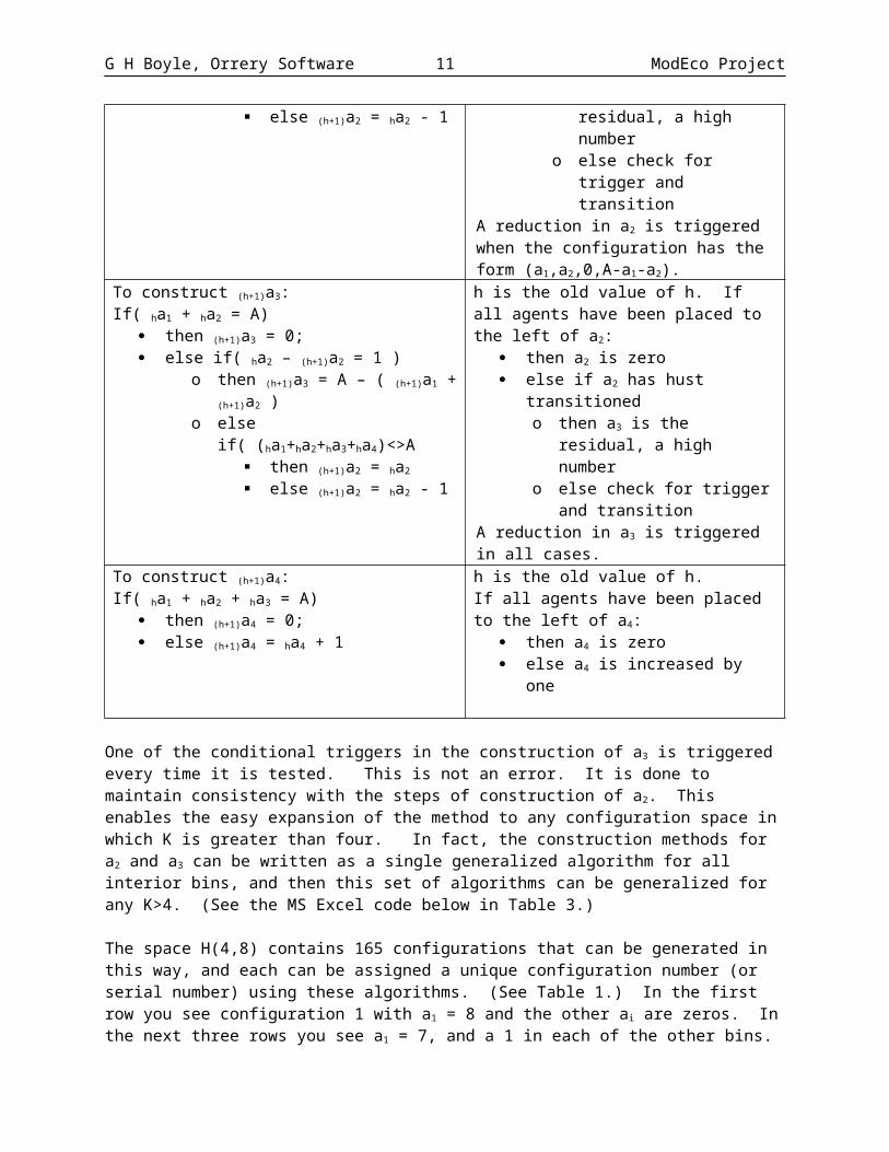
Given the hth configuration h(ha1,ha2,ha3,ha4) in H(4,A), the next configuration in the series can be constructed using the iterative transition rule described in Table 1. The number h plays two roles in the following algorithm. h is the serial number, but it is also an index number, used in a left-hand subscript, and used to distinguish the coordinates of one configuration from those of the next.

Table 1. The transition rule to iteratively construct an orderded list of all of the elements of H(4,A), given an initial element (A,0,0,0), where A = 4q for some positive integer q > 2.

Steps to take in construction Description of each stepTo construct a new serial number (new)h:(new)h = oldh + 1;

The new serial number (or configuration number) is one larger than the previous serial number.

To construct (h+1)a1:If( ha1 + ha4 = A)

then (h+1)a1 = ha1 – 1; else (h+1)a1 = ha1;

h is the old value of h. Methodically reduce the size of a1, triggered by the placement of all other agents in bin 4. A reduction in a1 is triggered when the configuration has the form (a1,0,0,A-a1).

To construct (h+1)a2:If( ha1 = A)

then (h+1)a2 = 0; else if( ha1 – (h+1)a1 = 1 )

o then (h+1)a2 = A – (h+1)a1

o else if( (ha1+ha2+ha4)<>A then (h+1)a2 = ha2

else (h+1)a2 = ha2 - 1

h is the old value of h. If all agents have been placed to the left of a2:

then a2 is zero else if a1 has just transitioned

o then a2 is the residual, a high number

o else check for trigger and transition

A reduction in a2 is triggered when the configuration has the form (a1,a2,0,A-a1-a2).


To construct (h+1)a3:If( ha1 + ha2 = A)

then (h+1)a3 = 0; else if( ha2 – (h+1)a2 = 1 )

o then (h+1)a3 = A – ( (h+1)a1 + (h+1)a2 )o else if( (ha1+ha2+ha3+ha4)<>A

then (h+1)a2 = ha2

else (h+1)a2 = ha2 - 1

h is the old value of h. If all agents have been placed to the left of a2:

then a2 is zero else if a2 has hust transitioned

o then a3 is the residual, a high number

o else check for trigger and transition

A reduction in a3 is triggered in all cases.To construct (h+1)a4:If( ha1 + ha2 + ha3 = A)

then (h+1)a4 = 0; else (h+1)a4 = ha4 + 1

h is the old value of h.If all agents have been placed to the left of a4:

then a4 is zero else a4 is increased by one

One of the conditional triggers in the construction of a3 is triggered every time it is tested. This is not an error. It is done to maintain consistency with the steps of construction of a2. This enables the easy expansion of the method to any configuration space in which K is greater than four. In fact, the construction methods for a2 and a3 can be written as a single generalized algorithm for all interior bins, and then this set of algorithms can be generalized for any K>4. (See the MS Excel code below in Table 3.)

The space H(4,8) contains 165 configurations that can be generated in this way, and each can be assigned a unique configuration number (or serial number) using these algorithms. (See Table 1.) In the first row you see configuration 1 with a1 = 8 and the other ai are zeros. In the next three rows you see a1 = 7, and a 1 in each of the other bins. And so on. It is possible to use Excel formulae to implement these algorithms and generate a complete table of all possible ways that A agents can be distributed across K bins.

Table 2. The first 10 rows of output from the configuration generation algorithms for H(K,A)=H(4,8). Each row can be interpreted as a 4-bin histogram, or as a 4-tuple.

Config No

Bin 1 Bin 2 Bin 3 Bin 4

h ha1 ha2 ha3 ha4

1 8 0 0 02 7 1 0 03 7 0 1 04 7 0 0 15 6 2 0 06 6 1 1 07 6 1 0 18 6 0 2 09 6 0 1 1

10 6 0 0 2


Note how the agents in the left-most bin appear to move towards the right-most bin as the transition rule is applied iteratively.

The MS Excel formulae that were used to implement the construction methods are lengthy but straightforward, and can be replicated as follows (See Table 3 for the cell entries.):

The first configuration is placed in row 7 in cells C7, D7, E7, F7 and G7 and the formulae placed into those cells are simply the initial values of h and of the a i, that is, the numbers 1, 8, 0, 0, and 0 (shaded pink).

Then the computational formulae shown in Table 3 (shaded blue) are entered into cells in row 8 of the spreadsheet.

Then select the five formulae in row 8 and drag them down to row 172. This will generate 165 unique configurations, each with a uniquely assigned configuration number (or serial number).

Table 3. The MS Excel formulae used to generate the configuration numbers and configurations for H(4,8). The notational symbols correspond to those used in Table 1.

Cell

Symbol Excel Formula

C7 1h 1D7 1a1 8E7 1a2 0F7 1a3 0G7 1a4 0C8 (j+1)h =C7+1D8 (j+1)a1 =IF(SUM($D7:D7)+$G7=$D$7,D7-1,D7)E8 (j+1)a2 =IF(SUM($D8:D8)=$D$7,0,IF(D7-D8=1,$D$7-SUM($D8:D8),IF(SUM($D7:E7)+$G7<>$D$7,E7,E7-1)))F8 (j+1)a3 =IF(SUM($D8:E8)=$D$7,0,IF(E7-E8=1,$D$7-SUM($D8:E8),IF(SUM($D7:F7)+$G7<>$D$7,F7,F7-1)))G8 (j+1)a4 =IF(SUM($D8:$F8)=$D$7,0,G7+1)

The number of points in the configuration space H(K,A) is given by the formula:

Card (H (K , A ))=(∏i=1K−1

( A+i ))/ (K−1 ) ! Equ (8)

where Card() is the counting function “cardinality”. Card(H(K,A)) rises more slowly than an exponential curve. For a relatively small histogram, the number of possible configurations is nevertheless enormous. For example, for a histogram with 30 bins (K=30) and 100 agents (A=100) the number of configurations exceeds 1028. Another version of the same formula, but one which is easier to implement in MS Excel, is:

Card (H (K , A ))= ( A+K−1 ) !A ! (K−1 )!

Equ (9)

6. Levels of Total Wealth in H(K,A) We distinguish between personal wealth level and total wealth level in the model. For any agent, its personal wealth level is xi corresponding to its assignment to bin i of the histogram. The total wealth level in the model, on the other hand, is found by summing the personal wealth over all agents to find w(h) as per equation 2.


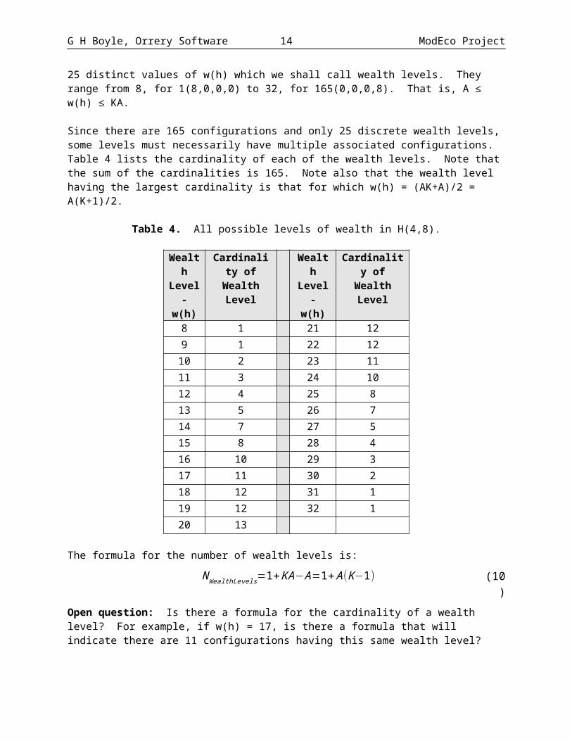
For all h H(K,A) there are many possible values for w(h). For example, if you list the 165 configurations for the H(4,8) configuration space and compute w(h) for each configuration, there are 25 distinct values of w(h) which we shall call wealth levels. They range from 8, for 1(8,0,0,0) to 32, for 165(0,0,0,8). That is, A ≤ w(h) ≤ KA.

Since there are 165 configurations and only 25 discrete wealth levels, some levels must necessarily have multiple associated configurations. Table 4 lists the cardinality of each of the wealth levels. Note that the sum of the cardinalities is 165. Note also that the wealth level having the largest cardinality is that for which w(h) = (AK+A)/2 = A(K+1)/2.

Table 4. All possible levels of wealth in H(4,8).

WealthLevel -w(h)

Cardinality of Wealth Level

WealthLevel -w(h)

Cardinality of Wealth Level

8 1 21 12

9 1 22 12

10 2 23 11

11 3 24 10

12 4 25 8

13 5 26 7

14 7 27 5

15 8 28 4

16 10 29 3

17 11 30 2

18 12 31 1

19 12 32 1

20 13

The formula for the number of wealth levels is:

NWealthLevels=1+KA−A=1+A (K−1) (10)

Open question: Is there a formula for the cardinality of a wealth level? For example, if w(h) = 17, is there a formula that will indicate there are 11 configurations having this same wealth level?

7. Levels of the Entropic Index in H(K,A) Unlike wealth, for which it is clear that each agent holds an identifiable quantity of wealth, it is not at all clear that an agent holds an identifiable quantity of entropy. Although it is mathematically possible to calculate the contribution of one agent to an indexical using s i/ai, we cannot say that an agent has a personal entropic index without reference to the entire state of the model in which the agent resides. But, similar to total wealth levels, if you calculate (using equation 3) the entropic index associated with all 165 configurations of H(4,8) you find that there are 15 distinctly different levels of entropic index.


That is, the entropic index can be used to categorize the configurations of the state space into 15 subsets, each subset having a cardinality, as shown in Table 5.

Table 5. All Possible Levels of The Entropic Index in H(4,8).

Entropic IndexLevel -

S(h)

Cardinality of Entropic Index

Level

Entropic IndexLevel -

S(h)

Cardinality of Entropic Index

Level

0.000000 4 0.750000 12

0.271782 12 0.774397 4

0.405639 12 0.780639 12

0.477217 12 0.875000 12

0.500000 6 0.905639 6

0.530639 12 0.952820 12

0.649397 24 1.000000 1

0.702820 24

Open Questions: Is there a formula that can be used to calculate the number of discrete levels of the entropic index for H(K,A)? For a given value of the entropic index, is there a formula that can be used to calculate the cardinality of the set of configurations having that entropic index?

8. Intersecting Levels in H(K,A) Figure 2 shows the scatter plot of S(h) vs. w(h) for all 165 configurations in H(4,8). There are several interesting things to note about this graph. The data points lie on a grid of intersecting horizontal and vertical lines, as is expected due to the finite number of discrete levels computable for each of the two variables. Many of the 165 data points overlay each other, so there are not 165 data points visible on the scatter plot. For each level of wealth, the maximal entropic index has been highlighted as a circled data point. A quadratic trend line (solid black line) has been included for these maximal values, with a corresponding equation and R2 value. These maximal values appear to be bounded by a curve forming a virtual envelope which, for the sake of discussion, we shall call the enveloping curve, or E-curve for H(K,A). Based on the shape of the trend line through the maximal values, this E-curve (dotted black line), is close to quadratic in shape, but is too narrow at the base and too blunt at the vertex. Also, if you examine the pattern of points within the interior area of the graph, the mind’s eye sees apparent arcs sweeping between basal points. These arcs are, in fact, scaled copies of the E-curve. Using a line drawing facility in MS Excel, a trace of the E-curve was made and then scaled and translated to fit two of the smaller apparent curves. They are the solid blue traces in the interior, both of which each pass precisely through several data points. It seems that the plotted points are located where a background set of continuous variously-scaled copies of the E-curve intersect with a grid of computed levels of wealth and computed levels of entropic index. Note also that the vertex occurs at configuration 69(2,2,2,2), the configuration that is distantly analogous to a state of thermodynamic equilibrium, having S(h) = 1.


Figure 2. A scatter plot showing S(h) (levels of entropic index) vs w(h) (levels of total wealth) for all 165 configurations in H(4,8). The maximal values of S(h) for each w(h) are circled, and a quadratic trend line through these maximal values is shown in black. The virtual enveloping curve (or E-Curve) is shown as a dotted black line. Two scaled and translated copies of the E-Curve are shown in solid blue in the interior area.

Open questions: What is the analytic expression for the E-curve which forms the upper bounding envelope of the possible values of the entropic index? What is the cause of the apparent self-similar pattern of overlays of this curve?

9. The H(K,A,W) Configuration Space Consider a specific configuration h(a1,a2,a3,a4) H(K,A,W) H(K,A) HRect(K,A). We define a nearest neighbor within the enveloping hypercube HRect(K,A) as a configuration which is a distance of one away from it. Distance is measured here in “Manhattan” distance units. If you change just one a i by ±1 then the new configuration is a nearest neighbor. This corresponds to adding or removing an agent. However, since there is a constraint within H(K,A) such that the sum of all a i must be A, this nearest neighbour is not in H(K,A). To be in the H(K,A) configuration space there must also be a compensating change in another bin. For example, if one is added to one bin, one must be subtracted from another bin. Therefore, for any h H(K,A) the nearest neighbor within H(K,A) must be a distance of two Manhattan steps away. This corresponds to removing an agent from a bin and then replacing the agent into a neighbouring bin. Since moving an agent from one bin to a neighbouring bin implicitly changes


the wealth they hold, to maintain constant wealth within the model, another agent must also move from bin to bin in the opposite direction, neutralizing the change in wealth. So, for any h H(K,A,W) the nearest neighbour within H(K,A,W) must be four Manhattan steps away.

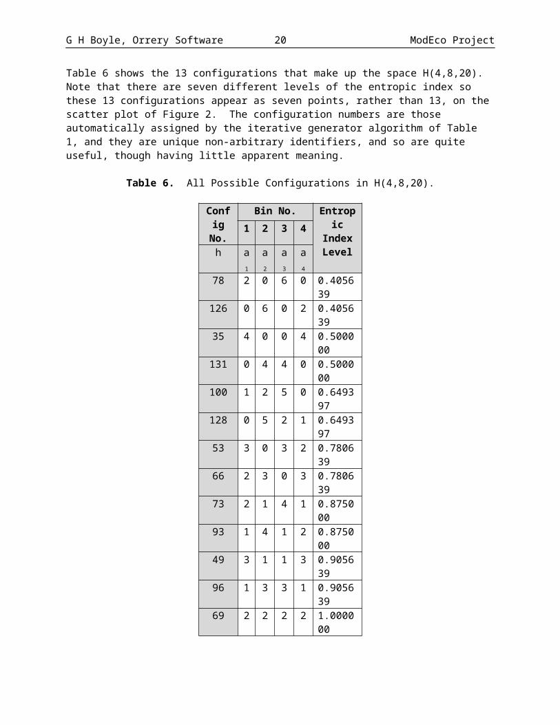
Returning to our example in which K=4 and A=8, in our capital exchange model, the total wealth is constant, at some value W. Suppose we set W = 20 when we initialize the model. Checking in Table 4 we see that there are only 13 configurations within H(4,8) which have this total wealth level. These 13 configurations then form the configuration space H(4,8,20) of the model. Our simple capital exchange model must operate within this type of highly constrained configuration space. We now turn our attention to examine the nature of this configuration space.

Within the capital exchange model two agents are always involved in every tick. When the loser moves one bin to the left (requiring two Manhattan steps), the winner moves one bin to the right (requiring two more Manhattan steps). The resultant configuration is a four-step Manhattan walk from the original configuration. However, the last two steps can retrace the path of the first two, so it is possible to end the walk at the original configuration. This would happen, for example, when a loser with $3 pays $1 to a winner with $2. The winner now has $3 and the loser now has $2. The agents have exchanged financial positions, as well as cash, and the overall wealth distribution has not changed. During a single tick of the model, all of the possible resultant configurations to be visited by our capital exchange model must be at a distance of 4 Manhattan steps from the current configuration.Call these four-step nearest neighbors “capital exchange nearest neighbours”. Call a pair of capital exhange nearest neighbours a “transition pair” because a single tick of the capital exchange model can transition the system from one member of this pair of configurations to the other, or back again in the next tick. As the capital exchange model operates, tick after tick, the system moves from configuration to configuration along paths formed by links between these transition pairs.

Hypothesis: All elements of the set H(K,A,W) form a single contiguous network of such transition pairs.

Hypothesis: The H(K,A) configuration space is formed by a set of non-overlapping H(K,A,W) sub-spaces that partition H(K,A).

For a given configuration h, how many capital exchange nearest neighbours are there? How many transition pairs does it belong to? How many resultant configurations can be visited in one tick? These are all different forms of the same equation. In a K-bin histogram in which all bins hold two or more agents there are K2 ways to choose two agents. This puts an upper limit on the possible number of transition pairs in which a configuration can be a partner. However, any selection of agents that chooses a loser from bin 1 or a winner from bin 4 results in no capital exchange, and no change of configuration. Of the K2 types of selection, only (K-1)2 are not disallowed by such a constraint. So, (K-1)2 is a more severe upper limit on the number of allowed transitions. Agents at the edges of the histogram have fewer opportunities to participate in the economy than those in the middle. Such constraints are called edge effects. Another type of edge effect occurs when a bin has 0 agents or 1 agent. These configurations have fewer than (K-1)2 allowed transitions. Edge effects will reduce this number for some configurations. With this variety of constraints, the number of transition pairs in which a configuration can be a partner varies.

In our example, when K = 4, each configuration will have, at most, 9 capital exchange nearest neighbors, but, since the H(4,8,20) space is very small, edge effects will reduce this number for most configurations.


Open question: Do these configurations in H(K,A,W) all lie on a (K-2) dimensional simplex?

Hypothesis: The H(K,A,W) space forms a Markov chain that is:• Time homogeneous – the probability of transition between the two configurations of a transition

pair does not change over time. Such probabilities are stable.• Memoryless – the next transition is dependent only on the current configuration and the set of

transition pairs of which it is a member, and is otherwise independent of previous transitions.• Irreducible – it is possible to get to any configuration from any configuration within the network.• Aperiodic – all configurations can be revisited in one or two ticks due to the fact that transitions are

bi-directional.

Table 6 shows the 13 configurations that make up the space H(4,8,20). Note that there are seven different levels of the entropic index so these 13 configurations appear as seven points, rather than 13, on the scatter plot of Figure 2. The configuration numbers are those automatically assigned by the iterative generator algorithm of Table 1, and they are unique non-arbitrary identifiers, and so are quite useful, though having little apparent meaning.

Table 6. All Possible Configurations in H(4,8,20).

Config No.

Bin No. Entropic IndexLevel1 2 3 4

h a1 a2 a3 a478 2 0 6 0 0.405639126 0 6 0 2 0.40563935 4 0 0 4 0.500000131 0 4 4 0 0.500000100 1 2 5 0 0.649397128 0 5 2 1 0.64939753 3 0 3 2 0.78063966 2 3 0 3 0.78063973 2 1 4 1 0.87500093 1 4 1 2 0.87500049 3 1 1 3 0.90563996 1 3 3 1 0.90563969 2 2 2 2 1.000000

10. Generating Transition PairsWe can use MS Excel to generate transition pairs with associated probabilities of transition for any subspace H(K,A,W) H(K,A) for which Card(H(K,A)) < 1,048,000, due to the limitations of MS Excell 2010. Unfortunately, very few interesting ABMs would meet this requirement. The technique is documented below in the expectation that a less restrictive version can ultimately be developed, possibly on another analytic platform.

We can define a K-tuple transition template as a symbol that designates one possible way to select a winner and a loser. W means the winner is chosen from this bin. L means the loser is chosen from this


bin. W/L means both winner and loser are chosen from the same bin. For a 4-bin model, there are four bins from which we can choose a winner, and four from which we can choose a loser, making 42 = 16 possible ways to choose the two. The sixteen 4-tuple transition templates are described in Table 7.

Table 7. The sixteen 4-tuple transition templates applicable to a generic configuration h H(4,A), A = 4q for some positive integer q > 2.

T# Template Discussion1 (W/L,-,-,-) Dissallowed; Loser is in bin 1.2 (L,W,-,-) Dissallowed; Loser is in bin 1.3 (L,-,W,-) Dissallowed; Loser is in bin 1.4 (L,-,-,W) Dissallowed; Loser is in bin 1; Winner is in bin 4.5 (W,L,-,-) Allowed; Reflexive; Winner and loser exchange situations.6 (-,W/L,-,-) Allowed.7 (-,L,W,-) Allowed.8 (-,L,-,W) Dissallowed; Winner is in bin 4.9 (W,-,L,-) Allowed.

10 (-,W,L,-) Allowed; Reflexive; Winner and loser exchange situations.11 (-,-,W/L,-) Allowed.12 (-,-,L,W) Dissallowed; Winner is in bin 4.13 (W,-,-,L) Allowed.14 (-,W,-,L) Allowed.15 (-,-,W,L) Allowed; Reflexive; Winner and loser exchange situations.16 (-,-,-,W/L) Dissallowed; Winner is in bin 4.

In general, if a configuration h has ai > 2 for all i, then: There are a total of K2 potential selections, of which:

o 2K-1 are disallowed, after selection; ando (K-1)2 are allowed, of which:

K-1 are valid exchanges which do not alter the histogram configuration; and (K-1)*(K-2) are valid transitions that change the configuration.

Note that the nature of the template does not determine the probability that its application will be instantiated when the winner and loser are randomly selected. For any given input configuration h, edge effects will reduce the number of templates that may be applicable, thus altering probabilities of application. For example, let’s examine the options for 78(2,0,6,0).

Due to the zeros in bins 2 and 4, those templates which indicate a selection from those bins will never be called up or applied to this configuration. So the following templates will never be activated for this configuration: 2, 4, 5, 6, 7, 8, 10, 12, 13, 14, 15, and 16. These templates have zero probability of being called up when the model is in configuration 78, thus increasing the probabilities of application of the other templates.

There are two ways to choose the two agents that result in no exchange: (L, ,W, ) and (W/L, , , ). Both result in no exchange because the loser has a single dollar and cannot give it away. There is a clear opportunity to select agents that fit this template, but the transitions are dissallowed.

There are only two allowed transitions. 78(2,0,6,0) transitions to 100(1,2,5,0) or it transitions to 73(2,1,4,1). A selection template can be constructed for each of these: (W, ,L, ) and ( , ,W/L, ) respectively.


The total count is 16.

What are the probabilities of such transitions? There are four ways to choose the two agents, only two of which cause a transition. Table 8 shows a transition table with the associated probability of selection for each of the four ways to choose two agents from 78(2,0,6,0). Note that the denominator of the probabilities is A*(A-1) = 8*7 = 56. There are two ways to choose a winner from bin 1, and 6 ways to choose a loser from bin 2. 2 * 6 = 12. So, the probability of transitioning from 78 to 100 is 12/56. Note that the probability of selecting a disallowed assignment of winner/loser combinations is not zero, so these non-effective results should be tabulated as part of the transition table for any configuration, as a technique to ensure that the probabilities have been correctly computed. The probabilities in such a transition table should always add to 1.000. Denote the weighted average entropic change for a configuration as the WAEC.

Table 8. Transition table for 78(2,0,6,0).

Winner/Loser Template

Probability of Selection (p)

Transition To

Delta Entropic Index (dEi) Computation of WAEI(p*dEi)

(W, -, L, - ) 12 / 56 100(1,2,5,0) 0.649397 – 0.405639 = +0.243758 0.052234(W/L, -, -, - ) 2 / 56 Disallowed 0.000000 0.000000(L, - W, - ) 12 / 56 Disallowed 0.000000 0.000000( -, -, W/L, - ) 30 / 56 73(2,1,4,1) 0.875000 – 0.405639 = +0.469360 0.251443 Total 56 / 56 0.303677

The weighted average entropic change (WAEC) for h(a1,a2,a3,a4) = 78(2, 0, 6, 0) is calculated as the sum of the probabilities times the respective deltas in the entropic index, and is 0.303677. Such a value might be useful in a computation of rates of entropy production. For configuration 78, all allowed transitions increase the entropic index, so there is no way but up.

Similar analysis can be done automatically for each of the 13 configurations in the H(4,8,20) space using an MS Excel table to generate the 16 template selections and their associated probabilities. Figure 3 shows the output for h = 78 with the results for all 16 templates. The templates marked with a ‘d’ are disallowed. The templates marked with an ‘s’ indicate an exchange of capital that does not change the configuration. A macro is used to cycle through the 13 input configurations. The output is collected in a large table having 13 * 16 = 208 entries, 140 of which are discardable due to edge effects. 68 retained records are then paired, to produce 34 descriptions of transition pairs.

Figure 3. A picture of the MS Excel table used to generate all 16 potential selections for transition for a configuration h in H(4,8,20). In this example, the input configuration has serial number h = 78.


Adjust Formulae in Red Cells Adjust Formulae in Red CellsS T U V W X Y Z AA AB AC AD AE

This Configuration:

Hash No: 1072 Config No: 78 A*(A-1) 56EM: 0.405639 WAEC: 0.30367730 WAEC = Weighted Average Entropic Change in transitions Probability

8 1 2 3 4 Transition Hash Config Entropic Entropic Probability of Times

7 Flag 2 0 6 0 Template Nos Nos Measure Change Transition Entropy

1 D D D D (W/L,-,-,-)d N/A N/A N/A 0.00000000 0.03571429 0.000000000 - - - - (W,L,-,-)s - - - - - -1 1 2 5 0 (W,-,L,-) 680 100 0.64939747 0.24375841 0.21428571 0.052233940 - - - - (W,-,-,L) - - - - - -0 - - - - (L,W,-,-)d - - - - - -1 D D D D (L,-,W,-)d N/A N/A N/A 0.00000000 0.21428571 0.000000000 - - - - (L,-,-,W)d - - - - - -0 - - - - (-,W/L,-,-) - - - - - -0 - - - - (-,W,L,-)s - - - - - -0 - - - - (-,W,-,L) - - - - - -0 - - - - (-,L,W,-) - - - - - -0 - - - - (-,L,-,W)d - - - - - -1 2 1 4 1 (-,-,W/L,-) 1121 73 0.87500000 0.46936094 0.53571429 0.251443360 - - - - (-,-,W,L)s - - - - - -0 - - - - (-,-,L,W)d - - - - - -0 - - - - (-,-,-,W/L)d - - - - - -

1.000000000 0.303677304

After a lengthy process, too lengthy to describe in detail here, that is mostly automatable using macros, these records can be formed into a table of transition pairs. Table 9 shows the output of this process in which the 34 transition pairs are detailed, showing transitions in both directions. For example, configuration 126 can transition to configuration 93 with a delta in the entropic index of 0.46936, with a probability of transtion of 0.53571. While 93 can transition in the opposite direction to 126 with the opposite delta in the entropic index, but with a much lower probability of 0.01786. The ratio is a ratio of probabilities, with the probability of increased entropic index as numerator.

Table 9. Transition pairs for H(4,8,20), sorted in order of the ratio of probabilities of transition.

From h1 To h2

Delta Entropic

Index

Proba-bility (Pup)

From h2 To h1

Delta Entropic

Index

Proba-bility (Pdown)

Ratio(Pup / Pdown)

126 to 93 0.46936 0.53571 93 to 126 -0.46936 0.01786 3078 to 73 0.46936 0.53571 73 to 78 -0.46936 0.01786 30

131 to 96 0.40564 0.28571 96 to 131 -0.40564 0.01786 1635 to 49 0.40564 0.28571 49 to 35 -0.40564 0.01786 16

128 to 96 0.25624 0.35714 96 to 128 -0.25624 0.05357 6.666667100 to 96 0.25624 0.35714 96 to 100 -0.25624 0.05357 6.666667

126 to 128 0.24376 0.21429 128 to 126 -0.24376 0.03571 678 to 100 0.24376 0.21429 100 to 78 -0.24376 0.03571 6128 to 93 0.22560 0.17857 93 to 128 -0.22560 0.03571 5100 to 73 0.22560 0.17857 73 to 100 -0.22560 0.03571 566 to 69 0.21936 0.16071 69 to 66 -0.21936 0.03571 4.553 to 69 0.21936 0.16071 69 to 53 -0.21936 0.03571 4.5

131 to 128 0.14940 0.21429 128 to 131 -0.14940 0.08929 2.4131 to 100 0.14940 0.21429 100 to 131 -0.14940 0.08929 2.4


66 to 49 0.12500 0.10714 49 to 66 -0.12500 0.05357 273 to 69 0.12500 0.21429 69 to 73 -0.12500 0.07143 393 to 69 0.12500 0.21429 69 to 93 -0.12500 0.07143 353 to 49 0.12500 0.10714 49 to 53 -0.12500 0.05357 266 to 93 0.09436 0.10714 93 to 66 -0.09436 0.07143 1.549 to 69 0.09436 0.16071 69 to 49 -0.09436 0.07143 2.2596 to 69 0.09436 0.16071 69 to 96 -0.09436 0.07143 2.2553 to 73 0.09436 0.10714 73 to 53 -0.09436 0.07143 1.573 to 96 0.03064 0.14286 96 to 73 -0.03064 0.10714 1.33333393 to 96 0.03064 0.14286 96 to 93 -0.03064 0.10714 1.333333

131 to 131 0.00000 0.28571 131 to 131 0.00000 0.28571 1128 to 128 0.00000 0.21429 128 to 128 0.00000 0.21429 1100 to 100 0.00000 0.21429 100 to 100 0.00000 0.21429 1

66 to 66 0.00000 0.10714 66 to 66 0.00000 0.10714 153 to 53 0.00000 0.10714 53 to 53 0.00000 0.10714 173 to 73 0.00000 0.14286 73 to 73 0.00000 0.14286 193 to 93 0.00000 0.17857 93 to 93 0.00000 0.17857 149 to 49 0.00000 0.12500 49 to 49 0.00000 0.12500 196 to 96 0.00000 0.26786 96 to 96 0.00000 0.26786 169 to 69 0.00000 0.21429 69 to 69 0.00000 0.21429 1

Note that the probability of transition is asymmetric for almost every transition pair. For example, the probability of a transition from configuration 78 to configuration 100 is six times as large as the probability of transition from configuration 100 to configuration 78. In fact the only transitions that have symmetric probability of transition are those that do not change the entropic index, that is, those that do not change the configuration. In every case, the transition that raises the entropic index is the more probable. For some transitions, the asymmetry is enormous.

This asymmetric probability of transition within transition pairs is one of the causes of the so-called “arrow of time”. As time proceeds, this ABM is driven towards a configuration having ever greater entropic index, and then the probability that it can ever escape from that condition of high entropic index is relatively low. It seems that, within the network of transition pairs, there is a monotonic gradient of entropic indices, associated with a monotonic gradient of probabilities of transition.

In the process that produced the above table, the WAEC was also tabulated and is shown in Table 10. Note that, for three configurations, the probabilities are slightly in favour of a decrease in the entropic index, while for some, the probabilities are greatly in favour of an increase. Does this imply that the equilibrium value of the entropic index is less than the maximal value?

Table 10. Weighted Average Entropic Change (WAEC) by configuration for h H(4,8,20).

h WAEC

69 -0.04700696 -0.026098


49 -0.00547193 0.00798473 0.00798453 0.05875766 0.058757

100 0.109756128 0.10975635 0.115897

131 0.17992478 0.303677

126 0.303677

11. Transition Matrix for the Markov Chain H(K,A,W)As a Markov chain, H(4,8,20) can be represented by a transition matrix in which the sum of the entries in each row add up to 1, implying certain transition. However, in the capital exchange model, many exchanges are disallowed, and a selected pair of agents may be discarded with no transition, so a simple compilation of probabilities as calculated in the “Neighbor Generator” algorithm (see figure 3) does not produce a standard type of transition matrix. To produce a standard transition matrix, the rows need to be normalized, by dividing each entry by the row sum. Table 11 is such a normalized transition matrix. Denote this matrix by M. To understand the effects of the normalization calculation, compare the probabilities of transition for h = 78 in Tables 8 and 11. In Table 11 we have the probabilities of the allowed transitions (only) divided by the sum of those probabilities.

Table 11. Transition matrix M1, showing the probability of transition from configuration to configuration.

From\To 35 49 53 66 69 73 78 93 96 100 126 128 131

35 0.00 1.00 0.00 0.00 0.00 0.00 0.00 0.00 0.00 0.00 0.00 0.00 0.0049 0.04 0.30 0.13 0.13 0.39 0.00 0.00 0.00 0.00 0.00 0.00 0.00 0.0053 0.00 0.22 0.22 0.00 0.33 0.22 0.00 0.00 0.00 0.00 0.00 0.00 0.0066 0.00 0.22 0.00 0.22 0.33 0.00 0.00 0.22 0.00 0.00 0.00 0.00 0.0069 0.00 0.13 0.06 0.06 0.38 0.13 0.00 0.13 0.13 0.00 0.00 0.00 0.0073 0.00 0.00 0.11 0.00 0.32 0.27 0.03 0.00 0.22 0.05 0.00 0.00 0.0078 0.00 0.00 0.00 0.00 0.00 0.71 0.00 0.00 0.00 0.29 0.00 0.00 0.0093 0.00 0.00 0.00 0.11 0.32 0.00 0.00 0.27 0.22 0.00 0.03 0.05 0.0096 0.00 0.00 0.00 0.00 0.21 0.14 0.00 0.14 0.35 0.07 0.00 0.07 0.02

100 0.00 0.00 0.00 0.00 0.00 0.20 0.04 0.00 0.41 0.24 0.00 0.00 0.10126 0.00 0.00 0.00 0.00 0.00 0.00 0.00 0.71 0.00 0.00 0.00 0.29 0.00128 0.00 0.00 0.00 0.00 0.00 0.00 0.00 0.20 0.41 0.00 0.04 0.24 0.10131 0.00 0.00 0.00 0.00 0.00 0.00 0.00 0.00 0.29 0.21 0.00 0.21 0.29

Such a matrix is called a one-step matrix. For example, the pink cell in Table 9 contains the probability that configuration 49 will transition to configuration 53 in one step. If we multiply M by itself, the resultant matrix M2 is a two-step matrix. The cell for row 49 and column 53 would then contain the probability that configuration 49 could transition to configuration 53 in two steps. If we continue and take M to a higher power, the matrix Mn approaches a stable value M asymptotically as n goes to


infinity. Table 12 shows the matrix M100. Note that in all columns all cells are now the same. This means that the overall probability distribution of the future state of the system is independent of the initial state, after sufficient ticks.

Table 12. Transition Matrix M100, showing the ultimate probability distribution of the model in its state space.

From\To 35 49 53 66 69 73 78 93 96 100 126 128 131

35 0.004 0.095 0.056 0.056 0.298 0.115 0.004 0.115 0.178 0.030 0.004 0.030 0.01449 0.004 0.095 0.056 0.056 0.298 0.115 0.004 0.115 0.178 0.030 0.004 0.030 0.01453 0.004 0.095 0.056 0.056 0.298 0.115 0.004 0.115 0.178 0.030 0.004 0.030 0.01466 0.004 0.095 0.056 0.056 0.298 0.115 0.004 0.115 0.178 0.030 0.004 0.030 0.01469 0.004 0.095 0.056 0.056 0.298 0.115 0.004 0.115 0.178 0.030 0.004 0.030 0.01473 0.004 0.095 0.056 0.056 0.298 0.115 0.004 0.115 0.178 0.030 0.004 0.030 0.01478 0.004 0.095 0.056 0.056 0.298 0.115 0.004 0.115 0.178 0.030 0.004 0.030 0.01493 0.004 0.095 0.056 0.056 0.298 0.115 0.004 0.115 0.178 0.030 0.004 0.030 0.01496 0.004 0.095 0.056 0.056 0.298 0.115 0.004 0.115 0.178 0.030 0.004 0.030 0.014

100 0.004 0.095 0.056 0.056 0.298 0.115 0.004 0.115 0.178 0.030 0.004 0.030 0.014126 0.004 0.095 0.056 0.056 0.298 0.115 0.004 0.115 0.178 0.030 0.004 0.030 0.014128 0.004 0.095 0.056 0.056 0.298 0.115 0.004 0.115 0.178 0.030 0.004 0.030 0.014131 0.004 0.095 0.056 0.056 0.298 0.115 0.004 0.115 0.178 0.030 0.004 0.030 0.014

All of the preceding analysis has been done using MS Excel. We now have a predictive “model”, using MS Excel, of the behaviour of “Model I” of the EiLab application. We can compare this with an actual run of an ABM and so validate the above analysis.

An interpretation of Table 12 is easiest using a bar graph. (See Figure 4.) The blue bars represent the data from table 10. On the other hand, Model I was run until over 200,000 allowed transitions were noted and the actual distribution of expressed states was recorded, and is represented by the red bars. Note that configuration 69, the “equilibrium” state, is the most probable state, but, in this very simple system, random perturbations can take the system out of pure equilibrium for a significant percentage of ticks (i.e. 70% of the time).

Figure 4. The predicted probability distribution of the configurations of Model I in the space H(4,8,20), computed as M100, and the empirically obtained probability distribution, as determined over more than 200,000 allowed transitions.


We are comparing two distinctly different computer models of a single stochastic process. One model is static and built using MS Excel. The other is a dynamic ABM built using C++. The technologies are radically different, as are the conceptual tools used to construct the models and analyze the results. Nevertheless, the results are dramatically similar, not to say indistinguishable from the perspective of statistical theory.

There is one other common means to view a Markov chain and that is as a directed graph. In Figure 6 we have a simplified directed graph of the configuration space H(4,8,20), in which all transitions are bidirectional. Note that there is only one way to get to configuration 35(4,0,0,4) and that is through 49(3,1,1,3) via a very low probability transition. The global and local minima (green coloured configurations) form a ratchet that makes it difficult for the system to return to the lowest value of the entropic index. These minima all have at least one co-ordinate equal to zero. These local cul-de-sacs ensure that many forays towards a low value of the entropic index are turned back. Such a structure helps to explain why the climb from lower entropic index to higher entropic index in larger systems tends to be monotonically increasing. This is the second cause of the “arrow of time”.

Hypothesis: H(K,A,W) spaces for which the ratio A / K ≤ 3 (arbitrarily) will have many such local minima, while those for which this ratio is larger will have relatively fewer.

Figure 6. A simplified directed graph of the configuration space H(4,8,20).


12. ConclusionsWe are now in a position to state two significant hypotheses. The first is analogous to the second law of thermodynamics, but is applicable to all stochastic ABMs without reference to either thermodynamic theory, or information theory.

López-Ruiz, Sañudo and Calbet (2009) showed that the probability distributions that are characteristic of entropy-driven processes can be developed from purely geometrical arguments. This work supports the idea that entropy is fundamentally a mathematical phenomenon having physical manifestations, and implies that entropy can be defined for ABMs, and so was an inspiration for this hypothesis.

MEP Hypothesis for ABMs: In any stochastic agent-based model (ABM) in which the number of agents is conserved and a measured variable characteristic of the agents (e.g. wealth) is also conserved, for all transactions as well as at the system level, a histogram displaying the distribution of that conserved quantity among the agents will exhibit a rising entropic index, which rises to a maximal value, and remains there, except for minor fluctuations.

In other words, the entropic index of a conserved quantity in a closed stochastic ABM will increase to a maximum value, in an analogous fashion to the rise of entropy in a closed thermodynamic system.

Martyushev (2010) proposed that the Maximum Entropy Production Principle (MEPP) is the appropriate version of the MEP to be applied to open systems as they approach stationary states far from


equilibrium. The MEPP has not yet been widely accepted as a real-world phenomenon, partly due to the difficulty of defining entropy production in an open system. However, when viewing the entropic index as a characteristic of a histogram, it becomes an easy matter to identify actions that alter the entropic index of the system, and then measure the rate of increase in the entropic index. I believe that the formulation of the entropic index described in this paper opens the way for serious study of the concept of the MEPP. In our example, if neither the number of agents, nor the total wealth are conserved in the capital exchange model, we can still calculate the change in entropy each time an agent is removed from or added to the system, or each time wealth is removed from or added to the system.

MEPP Hypothesis for ABMs: In any open stochastic agent-based model (ABM) in which a measured variable characteristic of the agents can be displayed as a histogram showing the distribution of that characteristic among the agents, the rate of increase of the entropic index will rise to a maximum, and will remain there, except for minor fluctuations.

It is believed that the study of the MEPP using agent-based models will eventually lead to insights that establish that this phenomenon plays a major role in the operation of all stochastic dynamic systems, including physical, chemical, biological, economic, social and informational systems.

AcknowledgmentsThe author acknowledges the contributions of Burke Brown and David Talbot who inspired many discussions on the nature of physical manifestations of mathematical phenomena. The author also acknowledges the help of Kevin Nhan and Andrew Cumberland, who provided feedback during the preparation of the preliminary notes and the preparation of the manuscript.

Conflict of InterestThe author declares no conflict of interest.

References and NotesBOULANGER, P., & Bréchet, T. (2005). Models for policy-making in sustainable development: The state of the art and perspectives for research. Ecological Economics, 55(3), 337-350.

BOYLE, G. H. (2013). A simple complete conservative sustainable agent-based model economy: Some hypotheses. Unpublished manuscript.

BOYLE, G. H. (2013). "ModEco and the PMM - A simple physically conservative complete sustainable economy." (Version 2). CoMSES Computational Model Library. Retrieved from: http://www.openabm.org/model/3613/version/2

CLAUSIUS, R. (1865). Über die wärmeleitung gasförmiger körper. Annalen der Physik, (125), 353-400.

DRĂGULESCU, A., & Yakovenko, V. M. (2000). Statistical mechanics of money. Eur. Phys. J. B., (17), 723-729.

HALL (Ed.) (1995). Maximum power: The ideas and applications of H. T. Odum. Niwot, Colorado, USA: University Press of Colorado.


LÓPEZ-RUIZ, R., Sañudo, J., & Calbet, X. (2009). Equiprobability, entropy, gamma distributions and other geometrical questions in multi-agent systems. Entropy, (11), 957-971. doi: 10.3390/e11040959

MARTYUSHEV, L. M. (2010). The maximum entropy production principle: two basic questions. Philosophical Transactions of the Royal Society B, (365), 1333-1334. doi: 10.1098/rstb.2009.0295

SHANNON, C. E. (1948). A mathematical theory of communication. Bell System Technical Journal, 27(July, October), 379-423, 623-656.

TRIBUS, M. (1961). Thermodynamics and thermostatics: An introduction to energy, information and states of matter, with engineering applications. Princeton: D. Van Nostrand Company Inc.

YAKOVENKO, V. M. (2010a). Statistical mechanics of money, debt, and energy consumption. Science and Culture, 76(9-10), 430-436. doi: arXiv:1008.2179

YAKOVENKO, V. M. (2010b). Statistical mechanics approach to the probability distribution of money. Informally published manuscript, Available from arXiv. (1007-5074v1).

Documents

orrery-software.webs.comorrery-software.webs.com/03-Software/03-B-EiLab/Doc… · Web vieworrery-software.webs.com