Orthogonal Neighborhood Preserving Projections: A

projection-based dimensionality reduction technique ∗

E. Kokiopoulou † Y. Saad‡

March 21, 2006

Abstract

This paper considers the problem of dimensionality reduction by orthogonal projec-tion techniques. The main feature of the proposed techniques is that they attempt topreserve both the intrinsic neighborhood geometry of the data samples and the globalgeometry. In particular we propose a method, named Orthogonal Neighborhood Pre-serving Projections, which works by first building an “affinity” graph for the data, ina way that is similar to the method of Locally Linear Embedding (LLE). However, incontrast with the standard LLE where the mapping between the input and the reducedspaces is implicit, ONPP employs an explicit linear mapping between the two. As a re-sult, handling new data samples becomes straightforward, as this amounts to a simplelinear transformation. We show how to define kernel variants of ONPP, as well as howto apply the method in a supervised setting. Numerical experiments are reported toillustrate the performance of ONPP and to compare it with a few competing methods.

1 Introduction

The problem of dimensionality reduction appears in many fields including data mining, ma-chine learning and computer vision, to name just a few. The goal of dimensionality reductionis to map the high dimensional samples to a lower dimensional space such that certain prop-erties are preserved. Usually, the property that is preserved is quantified by an objectivefunction and the dimensionality reduction problem is formulated as an optimization prob-lem. For instance, Principal Components Analysis (PCA) is a traditional linear techniquewhich aims at preserving the global variance and relies on the solution of an eigenvalue prob-lem involving the sample covariance matrix. Locally Linear Embedding (LLE) [7, 11] is anonlinear dimensionality reduction technique which aims at preserving the local geometriesat each neighborhood.

∗Work supported by NSF under grant DMS 0510131 and by the Minnesota Supercomputing Institute.†EPFL, LTS4 lab, Bat. ELE, Station 11; CH 1015 Lausanne; Switzerland. Email: ef-

frosyni.kokiopoulou@epfl.ch‡Department of Computer Science and Engineering; University of Minnesota; Minneapolis, MN 55455.

Email: saad@cs.umn.edu.

1

While PCA is good at preserving the global structure, it does not preserve the locality ofthe data samples. In this paper, a linear dimensionality reduction technique is advocated,which preserves the intrinsic geometry of the local neighborhoods. The proposed method,named Orthogonal Neighborhood Preserving Projections (ONPP), projects the high dimen-sional data samples on a lower dimensional space by means of a linear transformation V . Thedimensionality reduction matrix V is obtained by minimizing an objective function whichcaptures the discrepancy of the intrinsic neighborhood geometries in the reduced space. Ex-perimental evidence seems to indicate that this feature is crucial in preserving the globalgeometry as well, via the interaction of overlapping neighborhoods. In particular, this sug-gests that ONPP can be effectively used for data visualization purposes and that it may beviewed as a synthesis of PCA and LLE.

ONPP constructs a weighted k-nearest neighbor (k-NN) graph which models explicitlythe data topology. Similarly to LLE, the weights are built to capture the geometry ofthe neighborhood of each point. The linear projection step is determined by imposing theconstraint that each data sample in the reduced space is reconstructed from its neighbors bythe same weights used in the input space. However, in contrast to LLE, ONPP computesan explicit linear mapping from the input space to the reduced space. Note that in LLE themapping is implicit and it is not clear how to embed new data samples (see e.g. researchefforts by Bengio et al. [2]). In the case of ONPP the projection of a new data sample isstraightforward as it simply amounts to a matrix by vector product.

ONPP shares some properties with Locality Preserving Projections (LPP) [4]. Bothare linear dimensionality reduction techniques which construct the k-NN graph in order tomodel the data topology. However, our algorithm uses the optimal data-driven weights ofLLE which reflect the intrinsic geometry of the local neighborhoods, whereas the uniformweights (0/1) used in LPP aim at preserving locality without explicit consideration to thelocal geometric structure. Note that Gaussian weights can be used in LPP but these aresomewhat artificial and require the selection of an appropriate value of the parameter σ,the width of the Gaussian envelope. Although this issue is often overlooked, it is crucialfor the performance of the method and remains a serious handicap when using Gaussianweights. Experimental results suggest that ONPP is effective in conveying meaningful localand global geometric information from high dimensional samples to low dimensional ones. Asecond significant difference between LLE and ONPP, is that the latter forces the projectionto be orthogonal. In LLE, the projection is defined via a certain objective function, whoseminimization leads to eigenvectors of a generalized eigenvalue problem.

2 Dimensionality reduction by projection

Given a dataset X = [x1, x2, . . . , xn] ∈ Rm×n and the dimension d of the reduced space, withd ¿ m, the goal of dimensionality reduction is to produce a set Y which is an accuraterepresentation of X, but of smaller dimension. This can be achieved in different waysby selecting the type of the reduced dimension Y as well as the desirable properties to bepreserved. By type we mean whether we require that Y be simply a low-rank representationof X, or a data set in a vector space with fewer dimensions. Examples of properties to bepreserved include the global geometry, or neighborhood information.

2

Projection-based techniques consist of replacing the original data X by a matrix of theform

Y = V >X, where V ∈ Rm×d. (1)

Thus, each vector xi is replaced by yi = V >xi a member of the d-dimensional space Rd. IfV is a unitary matrix, then Y represents the orthogonal projection of X into the V -space.

The best known technique in this category is Principal Component Analysis (PCA).PCA computes V such that the variance of the projected vectors is maximized, i.e, V is themaximizer of

maxV ∈ Rm×d

V >V = I

∥

∥

∥

∥

∥

yi −1

n

n∑

j=1

yj

∥

∥

∥

∥

∥

2

2

, yi = V >xi.

As can be easily shown, the matrix V which maximizes the above quantity is simply theset of left singular vectors of the matrix X(I − 1

nee>), associated with the largest d singular

values (e is the vector of ones).

2.1 LPP and OLPP

Another related techniques is that of Locality Preserving Projections. LPP projects the dataso as to preserve a certain affinity graph constructed for the data. This graph can be definedfor example by taking a certain nearness measure and include all points within a radius ε ofa given vertex, to its adjacency list. Alternatively, one can include those k nodes that are thenearest neighbors to xi. The weights can be defined in different ways as well. Two commonchoices are weights of the heat kernel wij = exp(−‖xi −xj‖

22/t) or constant weights (wij = 1

if i and j are adjacent, wij = 0 otherwise). The adjacency graph along with these weightsdefines a matrix W whose entries are the weights wij’s which are nonzero only for adjacentnodes in the graph. Note that the entries of W are nonnegative and that W is sparse andsymmetric.

LPP defines the projected points in the form yi = V >xi by putting a high penalty formapping nearest neighbor nodes in the original graph to distant points in the projected data.Specifically, the objective function to be minimized is

Elpp =1

2

n∑

i,j=1

wij‖yi − yj‖22 (2)

Note that the matrix V is implicitly represented in the above function, through the depen-dence of the yis on V .

The following theorem expresses the above objective function as a trace.

Theorem 2.1 Let W be a certain symmetric affinity graph, and define D = diag(di) withdi =

∑nj=1 wij. Let the points yi be defined to be the columns of Y = V >X where V ∈ Rm×d.

Then the objective function (2) is equal to

Elpp = tr[Y (D − W )Y >] = tr[V >X(D − W )X>V ] (3)

3

Proof. By definition:

Elpp =1

2

n∑

i,j=1

wij‖yi − yj‖22

=1

2

n∑

i,j=1

wij(yi − yj)>(yi − yj)

=1

2

n∑

i,j=1

wijy>

i yi +1

2

n∑

i,j=1

wijy>

j yj −

n∑

i,j=1

wijy>

i yj

=n

∑

i,j=1

wijy>

i yi −n

∑

i,j=1

wijy>

i yj

=n

∑

i

diy>

i yi −n

∑

i,j=1

wijy>

i yj.

An observation will simplify the first term of the above expression:

n∑

i=1

diy>

i yi = tr(DY >Y ) = tr[Y DY >]

and similarly, for the second term we have

n∑

i,j=1

wijy>

i yj =n

∑

i

(Y ei)>

n∑

j=1

wjiyj

=n

∑

i

e>i Y >(Y W )ei

= tr[Y >(Y W )]

= tr[Y WY >] .

Putting these expressions together results in (3).

The matrix L ≡ D − W is the Laplacian of the weighted graph defined above. Note thate>L = 0, so L is singular.

In order to define the yis by minimizing (3), we need to add a constraint to V . Fromhere there are several ways to proceed depending on what is desired.

OLPP We can simply enforce the mapping to be orthogonal, i.e., we can impose the con-dition V >V = I. In this case the set V is the eingenbasis associated with the lowesteigenmodes of the matrix

Clpp = X(D − W )X> (4)

We refer to this first option as the method of Orthogonal Locality Preserving Projec-tions. It differs from the original LPP approach, which uses the next option.

4

LPP We can impose a condition of orthogonality on the projected set: Y Y > = I. Note thatthe rows of Y are orthogonal, which means that the d basis vectors in Rn on which thexi’s are projected are orthogonal. Alternatively, we can also impose an orthogonalitywith respect to the weight D: Y DY > = I. (This gives bigger weights to points yi’s forwhich di

∑

j wij is large).

ONPP to be discussed later uses an option that is close to the first one, but it replacesthe matrix D−W with a matrix that is quite different. The first option leads to the standardeigenvalue problem:

X(D − W )X>vi = λivi . (5)

The classical LPP option leads to the generalized eigenvalue problem.

X(D − W )Xvi = λiXDXvi. (6)

In both cases the smallest d eigenvalues and eigenvectors must be computed.A slight drawback of the scaling used by classical LPP is that the linear transformation

is no longer orthogonal. However, the weights can be redefined (in fact rescaled) a priori sothat the diagonal D becomes the identity. We found that the issue of scaling is an importantone.

An interesting connection can be made with PCA as was observed in [5]. Using a slightlydifferent argument from [5], suppose we take as W the (dense) matrix W = 1

nee>. This

simply puts the uniform weight 1/n to every single pair (i, j) for the full graph. In this case,D = I and the objective function in (4) becomes

Clpp = X

(

I −1

nee>

)

X> = Cpca

PCA compute the eigenvectors associated with the largest eigenvalues of a “global” (full)graph. In contrast, methods based on Locality Preservation (such as LPP) compute theeigenvectors associated with the smallest eigenvalues of a “local” (sparse) graph. PCA islikely to be better at conveying global structure, while methods based on preserving thegraph will be better at maintaining locality.

3 ONPP

The main idea of ONPP is to seek an orthogonal mapping of a given data set so as to bestpreserve a graph which describes the local geometry. It is in essence a variation of OLPPdiscussed earlier, in which the graph is constructed differently.

3.1 The nearest neighbor affinity graph

Consider a dataset represented by the columns of a matrix X = [x1, x2, . . . , xn] ∈ Rm×n.ONPP begins by building an affinity matrix by computing optimal weights which will relatea given point to its neighbors in some locally optimal way. This phase is identical with thatof LLE [7, 11]. The basic assumption is that each data sample along with its k nearest

5

neighbors (approximately) lies on a locally linear manifold. Hence, each data sample xi isreconstructed by a linear combination of its k nearest neighbors. The reconstruction errorsare measured by minimizing the objective function

E(W ) =∑

i

‖xi −∑

j

wijxj‖22. (7)

The weight wij represent the linear coefficient for reconstructing the sample xi from itsneighbors {xj}. The following constraints are imposed on the weights:

1. wij = 0, if xj is not one of the k nearest neighbors of xi;

2.∑

j wij = 1, that is xi is approximated by a convex combination of its neighbors.

Note that the second constraint on the row-sum is similar to rescaling the matrix W in theprevious section, so that it yields a D matrix equal to the identity.

In the case when wii ≡ 0, for all i, then the problem is equivalent to that of finding asparse matrix Z, (Z ≡ I − W>) with a specified sparsity pattern, which has ones on thediagonal and whose row-sums are all zero. It is interesting to note in passing that verysimilar problems are encountered when computing preconditioners by sparse approximateinverses, see, e.g., [9].

There is a simple closed-form expression for the weights. Observe at first that thisdetermination of the w′

ijs for a given point xi is a local one, in the sense that it only dependson xi and its nearest neighbors. Any algorithm for computing the weight will be fairlyinexpensive.

Call G the local Grammian matrix associated with point i. The entries of G are definedby

gpl = (xi − xp)>(xi − xl) ∈ Rk×k.

Thus, G contains the pairwise inner products among the neighbors of xi, given that theneighbors are centered with respect to xi. Denoting by X(i) a system of vectors consisting ofxi and its neighbors, we need to solve the least-squares (X(i) − xie

>)wi,: = 0 subject to theconstraint e>wi,: = 1. It can be shown that the solution wi,: of this constrained least squaresproblem is given by the following formula [7] using the inverse of G,

wi,: =G−1e

e>G−1e. (8)

(recall that e is the vector of all ones). The weights wij satisfy certain optimality prop-erties. They are invariant to rotations, scalings, and translations. As a consequence ofthese properties the affinity graph preserves the intrinsic geometric characteristics of eachneighborhood.

3.2 The algorithm

Assume that each data point xi ∈ Rm is mapped to a lower dimensional point yi ∈ Rd, d ¿m. Since LLE seeks to preserve the intrinsic geometric properties of the local neighborhoods,it assumes that the same weights which reconstruct the point xi by its neighbors in the high

6

dimensional space, will also reconstruct its image yi, by its corresponding neighbors, in thelow dimensional space. In order to compute the yi’s for i = 1, . . . , n, LLE employs theobjective function:

Φ(Y ) =∑

i

‖yi −∑

j

wijyj‖22. (9)

In this case the weights W are fixed and we need to minimize the above objective functionwith respect to Y = [y1, y2, . . . , yn] ∈ Rd×n.

Similar to the case of LPP and OLPP, we need to impose some constraints on the yis.This optimization problem is formulated under the following constraints in order to makethe problem well-posed:

1.∑

i yi = 0 i.e., the mapped coordinates are centered at the origin and

2. 1n

∑

i yiy>i = I, that is the embedding vectors have unit covariance.

LLE does not impose any specific other constraints on the projected points, it only aims atreproducing the graph. So the objective function (9) is minimized with the above constraintson Y .

Note that Φ(Y ) can be written Φ(Y ) = ‖Y − Y W>‖2F , so

Φ(Y ) = ‖Y (I − W>)‖2F = tr

[

Y (I − W>)(I − W )Y >]

(10)

The problem will amount to computing the d eigenvalues of the matrix M = (I − W>)(I −W>)>, and the associated eigenvectors.

In ONPP an explicit linear mapping from X to Y is imposed which is in the form (1).So we have yi = V >xi, i = 1, . . . , n for a certain matrix matrix V ∈ Rm×d to be determined.In order to determine the matrix V , ONPP imposes the constraint that each data sample yi

in the reduced space is reconstructed from its k neighbors by exactly the same weights as inthe input space. This means that we will minimize the same objective function (10) as inthe LLE approach, but now Y is restricted to being related to X by (1). When expressed interms of the unknown matrix V , the objective function becomes

Φ(Y ) = ‖V >X(I − W>)‖2F = tr

[

V >X(I − W>)(I − W )X>V]

. (11)

If we impose the additional constraint that the columns of V are orthonormal, i.e. V >V =I, then the solution V to the above optimization problem is the basis of the eigenvectorsassociated with the d smallest eigenvalues of the matrix

M = X(I − W>)(I − W )X> . (12)

The assumptions that were made when defining the weights wij at the beginning of thissection, imply that the matrix I − W is singular. In the case when m > n the matrix M ,which is of size m × m, is at most of rank n and it is therefore singular. In the case whenm ≤ n, M is not necessarily singular. However, we observed in practice that ignoring thesmallest eigenvalue of M , which is zero in theory, is helpful. Note that the correspondingeigenvector is not the trivial vector e as is the case in LLE. Note also that the embeddingvectors of LLE are obtained by computing the eigenvectors of matrix M associated with itssmallest eigenvalues.

7

Algorithm: ONPP

Input: Dataset X ∈ Rm×n and d: dimension ofreduced space.Output: Embedding vectors Y ∈ Rd×n.1. Compute the k nearest neighbors of data points.2. Compute the weights wij which give the best

linear reconstruction of each data point xi

by its neighbors (Equ. (8)).3. Compute the projected vectors yi = V >xi,

where V is determined by computing the d + 1eigenvectors of

M = X(I − W>)(I − W )X>

associated with smallest eigenvalues.

Table 1: The ONPP algorithm.

An important property of ONPP is that mapping new data points to the lower dimen-sional space is trivial once the matrix V is determined. Consider a new test data sample xt

that needs to be projected. The test sample is projected onto the subspace yt = V >xt usingthe dimensionality reduction matrix V . Therefore, the computation of the new projectionsimplifies to a matrix vector product.

In terms of Computational cost, the first part of ONPP consists of forming the k-NNgraph. This scales as O(n2). Its second part requires the computation of a few of thesmallest eigenvectors of M . Observe that in practice this matrix is not computed explicitly.Rather, iterative techniques are used to compute the corresponding smallest singular vectorsof matrix X(I −W )> [8]. The inner computational kernel of these techniques is the matrix-vector product which scales quadratically with the dimensions of the matrix at hand.

3.3 Discussion

We can also think of developing a technique based on enforcing an orthogonality relationshipbetween the projected points instead of the V ’s. Making the projection orthogonal will tendto preserve distances and so the overall geometry will be preserved. In contrast, imposingthe condition Y Y > = I, will lead to a criterion that is similar to that of PCA: the points yi

will tend to be different from one another (because of the orthogonality of the rows of Y ).This is precisely what LLE does. In essence, the main difference between LLE and ONPPis in the selection of the orthogonality to enforce.

The two optimization problems are shown below:

LLE : minY ∈Rm×d; Y Y >=I tr[Y MY >]ONPP : minY =V >X;V ∈Rm×d; V V >=I tr[Y MY >]

.

It is also possible to enforce a linear relation between the Y and X data, but requirethe same orthogonality as LLE. We will refer to this procedure as Neighborhood PreservingProjections (NPP). In NPP, the objective function is the same as with ONPP and is given

8

by (11). However, the constraint is now Y Y > = I which yields, V >XX>V = I. Whatthis means is that NPP is a linear variant of LLE which makes the same requirement onpreserving the affinity graph and obtaining a data set Y which satisfies Y Y > = I:

NPP : minY =V >X;V ∈Rm×d; Y Y >=I tr[Y MY >]

If we define G = XX>, then this leads to the problem,

minV ∈ Rm×d, V >GV =I

V >MV . (13)

The solution if the above problem can be obtained by solving the generalized eigenvalueproblem (V >M)v = λGv. We note that in practice, the vectors V obtained in this way needto be scaled, for example, so that their columns have unit 2-norms.

It is interesting to observe that the eigenvectors which will be found are actually gener-alized singular vectors of the pair [X(I − W>), X]. In contrast, ONPP requires (standard)left singular vectors of the matrix X(I − W>), whereas LLE requires left singular vectorsof I − W>. In the sequel we will focus primarily on ONPP, though the variations to bedescribed can be also be defined for LPP, OLPP, and NPP.

4 Supervised ONPP

ONPP can be implemented in either an unsupervised or a supervised setting. In the latercase where the class labels are available, ONPP can be modified appropriately and yield aprojection which carries not only geometric information but discriminating information aswell. In a supervised setting we first build the data graph G = (N,E), where the nodes Ncorrespond to data samples and an edge eij = (xi, xj) exists if and only if xi and xj belong tothe same class. In other words, we make adjacent those nodes (data samples) which belongto the same class. Notice that in this case one does not need to set the parameter k, thenumber of nearest neighbors, and the method becomes fully automatic.

Denote by c the number of classes and ni the number of data samples which belong to thei-th class. The data graph G consists of c cliques, since the adjacency relationship betweentwo nodes reflects their class relationship. This implies that with an appropriate reorderingof the columns and rows, the weight matrix W will have a block diagonal form where thesize of the i-th block is equal to the size ni of the i-th class. In this case W will be of thefollowing form,

W = diag(W1,W2, . . . ,Wc).

The weights Wi within each class are computed in the usual way, as described by equation(8). The rank of W defined above, is restricted as is explained by the following proposition.

Proposition 4.1 The rank of I − W is at most n − c.

Proof. Recall that the row sum of the weight matrix Wi is equal to 1, because of theconstraint (2). This implies that Wiei = ei, ei = [1, . . . , 1]> ∈ Rni . Thus, the following cvectors

e1 0 · · · 00 e2 · · · 00 0 · · · ec

,

9

are linearly independent and belong to the null space of I−W . Therefore, the rank of I−Wis at most n − c.

Consider now the case m > n where the number of samples (n) is less than their dimension(m). This case is known as the undersampled size problem. A direct consequence of theabove proposition is that in this case, the matrix M ∈ Rm×m will have rank at most n − c.In order to ensure that the resulting matrix M will be nonsingular, we may employ an initialPCA projection that reduces the dimensionality of the data vectors to n− c. Call VPCA thedimensionality reduction matrix of PCA. Then the ONPP algorithm is performed and thetotal dimensionality reduction matrix is given by

V = VPCAVONPP,

where VONPP is the dimensionality reduction matrix of ONPP.

5 Kernel ONPP

It is possible to formulate a kernelized version of ONPP. Kernels have been extensively usedin the context of Support Vector machines (SVMs) [12]. Essentially, a nonlinear mappingΦ : Rm → H is employed, where H is a certain high-dimensional feature space. Denote byΦ(X) = [Φ(x1), Φ(x2), . . . , Φ(xn)] the transformed dataset in H.

The main idea of Kernel ONPP rests on the premise that the transformation Φ is onlyknown through its Grammian on the data X. In other words, what is known is the matrixK whose entries are

Kij ≡ k(xi, xj) = 〈Φ(xi), Φ(xj)〉. (14)

This is the Gram matrix induced by the kernel k(x, y) associated with the feature space. Infact, another interpretation of the Kernel mapping is that we are defining an alternative innerproduct in the X-space, which is defined through the inner product of every pair (xi, xj) as< xi, xj >= kij.

Formally, ONPP can be realized in a kernel form by simply applying it to the set Φ(X).Observe first that

K ≡ Φ(X)>Φ(X) . (15)

There are two implications of this definition. The first is that the mapping W has to bedefined using this new inner product. The second is that the optimization problem too hasto take the inner product into account.

Consider first the graph definition. In the feature space we would like to minimize

m∑

i=1

‖Φ(xi) −∑

j

wijΦ(xj)‖22.

This is the same as the cost function (7) evaluated on the set Z ≡ Φ(X) as desired, andtherefore an alternative expression for it is

E(W ) = ‖Φ(X)(I − W>)‖2F

= tr[(I − W )Φ(X)>Φ(X)(I − W>)]

= tr[(I − W )K(I − W>)]

10

Note that K is dense and n× n. The easiest way to solve the above problem is to extract alow rank approximation to the Grammian K, e.g.,

K = US2U> = (US)(US)>

Where W ∈ Rm×k and S ∈ Rk×k. Then the above problem becomes one of minimizing

tr(I − W )USSU>(I − W )> = ‖(I − W )US‖2F = ‖SU>(I − W>)‖2

F .

Therefore, SU> replaces X when constructing W .Consider now the problem of obtaining the projection matrix V in a kernel framework.

Observe that if we were to work in feature space, then we would take YΦ = V >Φ(X), whereV ∈ RL×d, where L is the (typically large and unknown) dimension of the feature space.Now the cost function (11) would become

tr[

V >Φ(X)(I − W>)(I − W )Φ(X)>V]

. (16)

Since Φ(X) is not explicitly known (and is of large dimension) this direct approach does notwork.

The first way out is to restrict V to be in the range of Φ(X). This is natural since eachcolumn of V is in RL the row-space of Φ(X). Specifically, we write V = Φ(X)Z whereZ ∈ Rm×d and Z>Z = I. Then (16) becomes

tr[

Z>Φ(X)>Φ(X)(I − W>)(I − W )Φ(X)>Φ(X)Z]

= tr[

Z>KMKZ]

. (17)

In a supervised setting, we need to project a test point xt onto the space of lower di-mension. The dot product of xt with all low dimensional basis vectors Φ(X)Z is computedas

Z>Φ(X)>Φ(xt) = Z>K(:, xt) . (18)

Here matlab notation is used so K(:, xt) represents the vector (k(xj, xt))j=1:n.It is somewhat unnatural to have the matrix K be involved quadratically in the expression

(17). Equations (16) suggests that we should really obtain K not K2, since Φ(X)>Φ(X) =K. For example if W ≡ 0, then (16) would become tr(V >KV ) whereas (17) would yieldtr(Z>K2Z). The second solution is to involve an implicit polar decomposition of Φ(X):

Φ(X) = QS with S = (Φ(X)>Φ(X))1/2 Q>Q = I . (19)

Note that Q is now an orthogonal basis of the range of Φ(X), and in this case, when V = QZthen (16) becomes

tr[

Z>Q>QS(I − W>)(I − W )SQ>QZ]

= tr[

Z>S(I − W>)(I − W )SZ]

. (20)

It is not necessary to compute S = K1/2 because the above problem can be solved as ageneralized eigenvalue problem instead. Let us set V∗ = SZ. Then

minZ ∈Rm×d,Z>Z=I

tr[

Z>S(I − W>)(I − W )SZ]

= minV∗ ∈Rm×d,V >

∗ KV∗=Itr

[

V >

∗ (I − W>)(I − W )V∗

]

.

11

This minimization can be achieved by solving the eigenvalue problem

(I − W>)(I − W )v = λKv.

Now the inner product of xt with all low dimensional basis vectors QZ becomes (recallthat V∗ = SZ, Q = Φ(X)S−1, and that S is symmetric)

Z>Q>Φ(xt) = Z>S−1Φ(X)>Φ(xt)

= Z>S−1S−1Φ(X)>Φ(xt)

= V >

∗ K−1 K(:, xt) . (21)

Matlab notation is used again so K(:, xt) represents the vector (k(xj, xt))j=1:n.Now consider for simplicity the case d = 1. Concerning the training points, observe that

the projections along the eigenvector v are given by y = Ka. Then, notice that minimiz-ing the trace (17) amounts to minimizing y>My which leads to the exact same eigenvalueproblem solved by LLE. Therefore, LLE (nonlinear) could be viewed as performing ONPP(linear) implicitly in the feature space H.

6 Experimental Results

In this section we evaluate all four linear dimensionality reduction methods LPP, NPP,OLPP and ONPP. We use an implementation of LPP which is publicly available1. Theimplementation of OLPP is based on a slight modification of the publically available LPPcode.

6.1 Synthetic data

−10

1 02

46−1

−0.5

0

0.5

1

1.5

2

2.5

3

Random points on a 3−D S−curve

−100

1020

010

2030

−15

−10

−5

0

5

10

15

Random points on a Swissroll

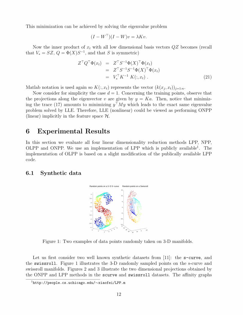
Figure 1: Two examples of data points randomly taken on 3-D manifolds.

Let us first consider two well known synthetic datasets from [11]: the s-curve, andthe swissroll. Figure 1 illustrates the 3-D randomly sampled points on the s-curve andswissroll manifolds. Figures 2 and 3 illustrate the two dimensional projections obtained bythe ONPP and LPP methods in the scurve and swissroll datasets. The affinity graphs

1http://people.cs.uchicago.edu/∼xiaofei/LPP.m

12

−1 0 1 2 3

−2

−1

0

1

ONPP

−2 −1 0 1 2 3−1.5

−1

−0.5

0

0.5

1

1.5

NPP

0 2 4−3

−2

−1

0

1

2

3

LPP

−1 0 1 2−3

−2

−1

0

1

OLPP

Figure 2: Results of four related methods applied to the S-curve example.

were all constructed using k = 10 nearest neighbor points. Observe that the performance ofLPP parallels that of NPP and, similarly, the performance of OLPP parallels that of ONPP.Note that all methods preserve locality which is indicated by the color shading. However,the orthogonal methods i.e., OLPP and ONPP preserve global geometric characteristics aswell, since they give a faithful projections which convey information about how the manifoldis folded in the high dimensional space.

6.2 Digit visualization

The next experiment involves digit visualization. We use 20×16 images of handwritten digitswhich are publically available from S. Roweis’ web page2. The dataset contains 39 samplesfrom each class (digits from ’0’-’9’). Each digit image sample is represented lexicographicallyas a high dimensional vector of length 320. For the purpose of comparison with PCA, wefirst project the dataset in the two dimensional space using PCA and the results are depictedin Figure 4. In the sequel we project the dataset in two dimensions using all four methods.The results are illustrated in Figures 5 (digits ’0’-’4’) and 6 (digits ’5’-’9’). We use k = 6 forconstructing the affinity graphs of all methods.

Observe that the projections of PCA are spread out since PCA aims at maximizing thevariance. However, the classes of different digits seem to heavily overlap. This means thatPCA is not well suited for discriminating between data. On the other hand, observe thatall the four graph-based methods yield more meaningful projections since samples of thesame class are mapped close to each other. This is because these methods aim at preservinglocality. Finally, ONPP seems to provide slightly better projections than the other methodssince its clusters appear more cohesive.

2http://www.cs.toronto.edu/∼roweis/data.html

13

−10 −5 0 5 10 15

−10

−5

0

5

10

15

ONPP

−10 0 10

−10

−5

0

5

10

NPP

−20 −10 0

−15

−10

−5

0

5

10

15

LPP

−10 −5 0 5 10 15

−10

−5

0

5

10

OLPP

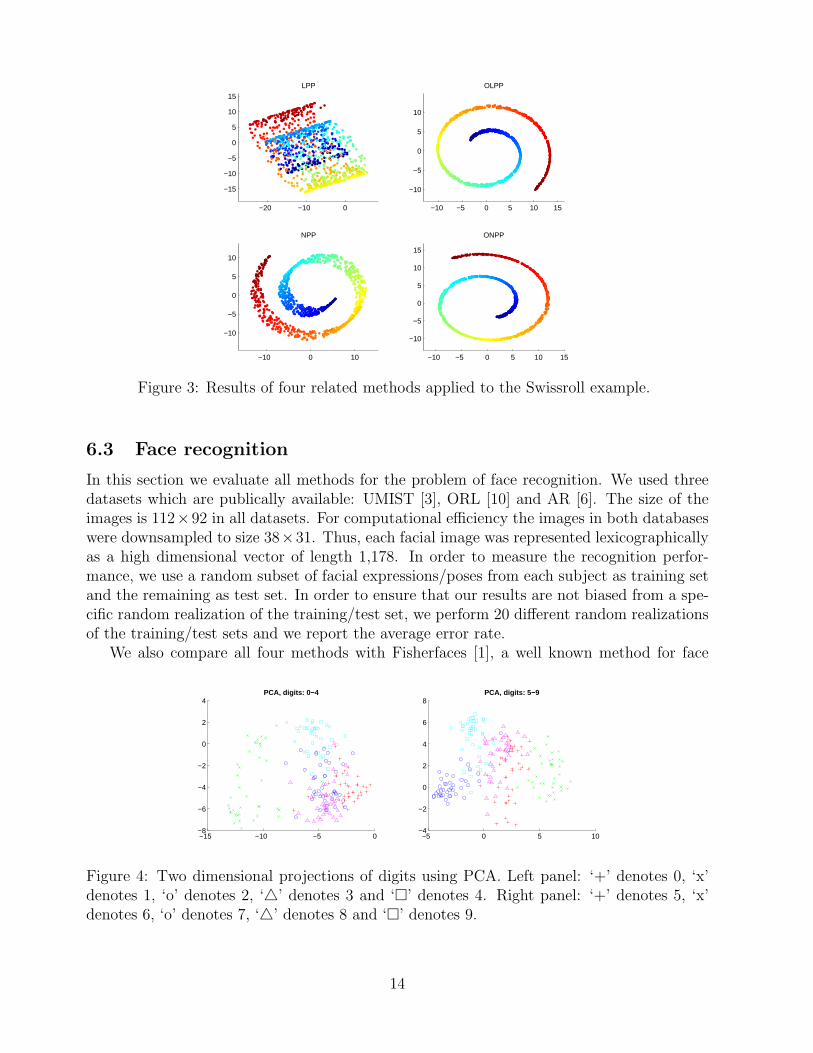
Figure 3: Results of four related methods applied to the Swissroll example.

6.3 Face recognition

In this section we evaluate all methods for the problem of face recognition. We used threedatasets which are publically available: UMIST [3], ORL [10] and AR [6]. The size of theimages is 112×92 in all datasets. For computational efficiency the images in both databaseswere downsampled to size 38×31. Thus, each facial image was represented lexicographicallyas a high dimensional vector of length 1,178. In order to measure the recognition perfor-mance, we use a random subset of facial expressions/poses from each subject as training setand the remaining as test set. In order to ensure that our results are not biased from a spe-cific random realization of the training/test set, we perform 20 different random realizationsof the training/test sets and we report the average error rate.

We also compare all four methods with Fisherfaces [1], a well known method for face

−15 −10 −5 0−8

−6

−4

−2

0

2

4PCA, digits: 0−4

−5 0 5 10−4

−2

0

2

4

6

8PCA, digits: 5−9

Figure 4: Two dimensional projections of digits using PCA. Left panel: ‘+’ denotes 0, ‘x’denotes 1, ‘o’ denotes 2, ‘4’ denotes 3 and ‘¤’ denotes 4. Right panel: ‘+’ denotes 5, ‘x’denotes 6, ‘o’ denotes 7, ‘4’ denotes 8 and ‘¤’ denotes 9.

14

−0.5 0 0.5 1−1

−0.5

0

0.5

1NPP, digits: 0−4

−0.5 0 0.5 1 1.5−2

−1.5

−1

−0.5

0ONPP, digits: 0−4

0.5 1 1.5 2 2.5 3−0.6

−0.4

−0.2

0

0.2

0.4

0.6

0.8

1LPP, digits: 0−4

−0.4 −0.2 0 0.2 0.4 0.6−0.3

−0.2

−0.1

0

0.1

0.2

0.3

0.4OLPP, digits: 0−4

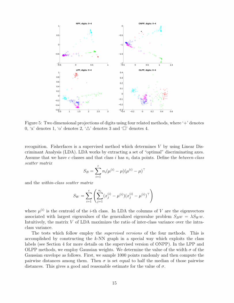
Figure 5: Two dimensional projections of digits using four related methods, where ‘+’ denotes0, ‘x’ denotes 1, ‘o’ denotes 2, ‘4’ denotes 3 and ‘¤’ denotes 4.

recognition. Fisherfaces is a supervised method which determines V by using Linear Dis-criminant Analysis (LDA). LDA works by extracting a set of “optimal” discriminating axes.Assume that we have c classes and that class i has ni data points. Define the between-classscatter matrix

SB =c

∑

i=1

ni(µ(i) − µ)(µ(i) − µ)>

and the within-class scatter matrix

SW =c

∑

i=1

(

ni∑

j=1

(x(i)j − µ(i))(x

(i)j − µ(i))>

)

where µ(i) is the centroid of the i-th class. In LDA the columns of V are the eigenvectorsassociated with largest eigenvalues of the generalized eigenvalue problem SBw = λSW w.Intuitively, the matrix V of LDA maximizes the ratio of inter-class variance over the intra-class variance.

The tests which follow employ the supervised versions of the four methods. This isaccomplished by constructing the k-NN graph in a special way which exploits the classlabels (see Section 4 for more details on the supervised version of ONPP). In the LPP andOLPP methods, we employ Gaussian weights. We determine the value of the width σ of theGaussian envelope as follows. First, we sample 1000 points randomly and then compute thepairwise distances among them. Then σ is set equal to half the median of those pairwisedistances. This gives a good and reasonable estimate for the value of σ.

15

−2 −1.5 −1 −0.5 0 0.5−1.5

−1

−0.5

0

0.5

1NPP, digits: 5−9

−1.5 −1 −0.5 0 0.5 1−2

−1.5

−1

−0.5

0

0.5

1ONPP, digits: 5−9

−2.5 −2 −1.5 −1 −0.5−1

−0.5

0

0.5

1

1.5

2LPP, digits: 5−9

−0.2 0 0.2 0.4 0.6−0.4

−0.2

0

0.2

0.4

0.6

0.8

1OLPP, digits: 5−9

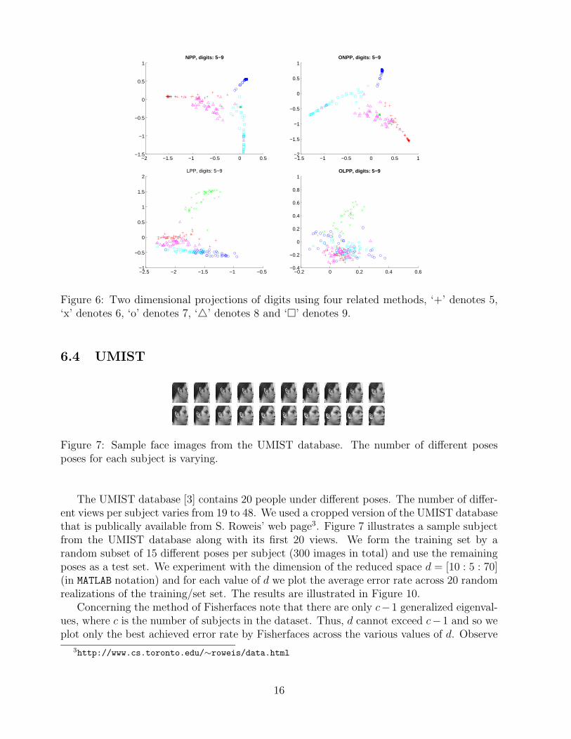
Figure 6: Two dimensional projections of digits using four related methods, ‘+’ denotes 5,‘x’ denotes 6, ‘o’ denotes 7, ‘4’ denotes 8 and ‘¤’ denotes 9.

6.4 UMIST

Figure 7: Sample face images from the UMIST database. The number of different posesposes for each subject is varying.

The UMIST database [3] contains 20 people under different poses. The number of differ-ent views per subject varies from 19 to 48. We used a cropped version of the UMIST databasethat is publically available from S. Roweis’ web page3. Figure 7 illustrates a sample subjectfrom the UMIST database along with its first 20 views. We form the training set by arandom subset of 15 different poses per subject (300 images in total) and use the remainingposes as a test set. We experiment with the dimension of the reduced space d = [10 : 5 : 70](in MATLAB notation) and for each value of d we plot the average error rate across 20 randomrealizations of the training/set set. The results are illustrated in Figure 10.

Concerning the method of Fisherfaces note that there are only c−1 generalized eigenval-ues, where c is the number of subjects in the dataset. Thus, d cannot exceed c−1 and so weplot only the best achieved error rate by Fisherfaces across the various values of d. Observe

3http://www.cs.toronto.edu/∼roweis/data.html

16

Figure 8: Sample face images from the ORL database. There are 10 available facial expres-sions and poses for each subject.

Figure 9: Sample face images from the AR database.

again that NPP and LPP have similar performance and that ONPP competes with OLPPand they both outperform the other methods across all values of d. We also report the besterror rate achieved by each method and the corresponding dimension d of the reduced space.The results are tabulated in the left portion of Table 2. Notice that PCA works surprisinglywell in this database.

10 20 30 40 50 60 700

1

2

3

4

5

6UMIST

dimension of reduced space

erro

r ra

te (

%)

LPPOLPPPCAONPPNPPLDA

Figure 10: Error rate with respect to the reduced dimension d. Top panel: UMIST databaseand bottom panel: AR database.

6.5 ORL

The ORL (formerly Olivetti) database [10] contains 40 individuals and 10 different imagesfor each individual including variation in facial expression (smiling/non smiling) and pose.Figure 8 illustrates two sample subjects of the ORL database along with variations in facialexpression and pose. We form the training set by a random subset of 5 different facial

17

0 50 100 1505

10

15

20

25

30

35

40

45ORL

dimension of reduced space

erro

r ra

te (

%)

LPPOLPPPCAONPPNPPLDA

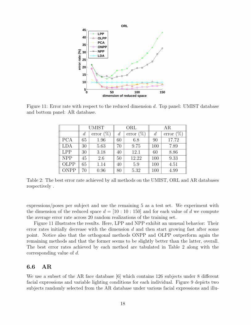
Figure 11: Error rate with respect to the reduced dimension d. Top panel: UMIST databaseand bottom panel: AR database.

UMIST ORL ARd error (%) d error (%) d error (%)

PCA 65 1.96 60 6.8 90 17.72LDA 30 5.63 70 9.75 100 7.89LPP 30 3.18 40 12.1 60 8.86NPP 45 2.6 50 12.22 100 9.33OLPP 65 1.14 40 5.9 100 4.51ONPP 70 0.96 80 5.32 100 4.99

Table 2: The best error rate achieved by all methods on the UMIST, ORL and AR databasesrespectively .

expressions/poses per subject and use the remaining 5 as a test set. We experiment withthe dimension of the reduced space d = [10 : 10 : 150] and for each value of d we computethe average error rate across 20 random realizations of the training set.

Figure 11 illustrates the results. Here, LPP and NPP exhibit an unusual behavior: Theirerror rates initially decrease with the dimension d and then start growing fast after somepoint. Notice also that the orthogonal methods ONPP and OLPP outperform again theremaining methods and that the former seems to be slightly better than the latter, overall.The best error rates achieved by each method are tabulated in Table 2 along with thecorresponding value of d.

6.6 AR

We use a subset of the AR face database [6] which contains 126 subjects under 8 differentfacial expressions and variable lighting conditions for each individual. Figure 9 depicts twosubjects randomly selected from the AR database under various facial expressions and illu-

18

30 40 50 60 70 80 90 1000

5

10

15

20

25

30AR

dimension of reduced space

erro

r ra

te (

%)

LPPOLPPPCAONPPNPPLDA

Figure 12: Error rate with respect to the reduced dimension d. Top panel: UMIST databaseand bottom panel: AR database.

mination. We form the training set by a random subset of 4 different facial expressions/posesper subject and use the remaining 4 as a test set. We plot the error rate across 20 randomrealizations of the training/test set, for d = [30 : 10 : 100].

The results are illustrated in Figure 12. Once again we observe that ONPP and OLPPoutperform the remaining methods across all values of d. In addition, notice that NPP hasparallel performance with LPP and they are both inferior to Fisherfaces. Furthermore, Table2 reports the best achieved error rate and the corresponding value of d. Finally, observe thatfor this database, PCA does not perform too well. In addition, OLPP and ONPP yield verysimilar performances for this case.

The above experimental results suggest that the orthogonality of the columns of thedimensionality reduction matrix V is very important for data visualization purposes. Thisis more evident in the case of face recognition, where this particular feature turned out tobe crucial for the performance of the method at hand.

7 Conclusion

The Orthogonal Neighborhood Preserving Projections (ONPP) introduced in this paper is alinear dimensionality reduction technique, which will tend to preserve not only the localitybut also the local and global geometry of the high dimensional data samples. It can beextended to a supervised method and it can also be combined with kernel techniques. Weintroduced three methods with parallel characteristics and compared their performance inboth synthetic and real life datasets. We showed that ONPP and OLPP can be very effectivefor data visualization, and that they can be implemented in a supervised setting to yield arobust recognition technique.

19

Acknowledgements We are grateful to Prof. D. Boley for his valuable help and insightfuldiscussions on various aspects of the paper.

References

[1] P. Belhumeur, J. Hespanha, and D. Kriegman. Eigenfaces vs. Fisherfaces: RecognitionUsing Class Specific Linear Projection. IEEE Trans. Pattern Analysis and MachineIntelligence, Special Issue on Face Recognition, 19(7):711—20, July 1997.

[2] Y. Bengio, J-F Paiement, P. Vincent, O. Delalleau, N. Le Roux, and M. Ouimet. Out-of-Sample Extensions for LLE, Isomap, MDS, Eigenmaps, and Spectral Clustering. InSebastian Thrun, Lawrence Saul, and Bernhard Scholkopf, editors, Advances in NeuralInformation Processing Systems 16. MIT Press, Cambridge, MA, 2004.

[3] D. B Graham and N. M Allinson. Characterizing Virtual Eigensignatures for GeneralPurpose Face Recognition. Face Recognition: From Theory to Applications, 163:446–456, 1998.

[4] X. He and P. Niyogi. Locality preserving projections. Advances in Neural InformationProcessing Systems 16 (NIPS 2003), 2003. Vancouver, Canada.

[5] X. He, S. Yan, Y. Hu, P. Niyogi, and H-J Zhang. Face recognition using Laplacianfaces.IEEE TPAMI, 27(3):328–340, March 2005.

[6] A.M. Martinez and R. Benavente. The AR Face Database. Technical report, CVC no.24, 1998.

[7] S. Roweis and L. Saul. Nonlinear Dimensionality Reduction by Locally Linear Embed-ding. Science, 290:2323–2326, 2000.

[8] Y. Saad. Numerical Methods for Large Eigenvalue Problems. Halstead Press, New York,1992.

[9] Y. Saad. Iterative Methods for Sparse Linear Systems, 2nd edition. SIAM, Philadelpha,PA, 2003.

[10] F. Samaria and A. Harter. Parameterisation of a Stochastic Model for Human FaceIdentification. In 2nd IEEE Workshop on Applications of Computer Vision, SarasotaFL, December 1994.

[11] L. Saul and S. Roweis. Think Globally, Fit Locally: Unsupervised Learning of NonlinearManifolds. Journal of Machine Learning Research, 4:119–155, 2003.

[12] V. Vapnik. Statistical Learning Theory. Wiley, New York, 1998.

20