OS6- 1

Chapter 6 CPU Scheduling

OS6- 2

OutlineBasic ConceptsScheduling Criteria Scheduling AlgorithmsMultiple-Processor SchedulingReal-Time SchedulingAlgorithm Evaluation

OS6- 3

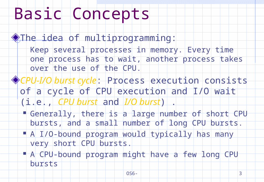
Basic ConceptsThe idea of multiprogramming:

Keep several processes in memory. Every time one process has to wait, another process takes over the use of the CPU.

CPU-I/O burst cycle: Process execution consists of a cycle of CPU execution and I/O wait (i.e., CPU burst and I/O burst) . Generally, there is a large number of short CPU

bursts, and a small number of long CPU bursts. A I/O-bound program would typically has many very

short CPU bursts. A CPU-bound program might have a few long CPU

bursts

OS6- 4

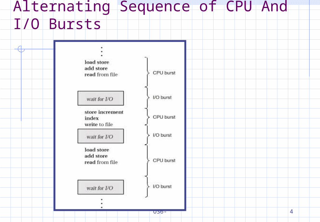
Alternating Sequence of CPU And I/O Bursts

OS6- 5

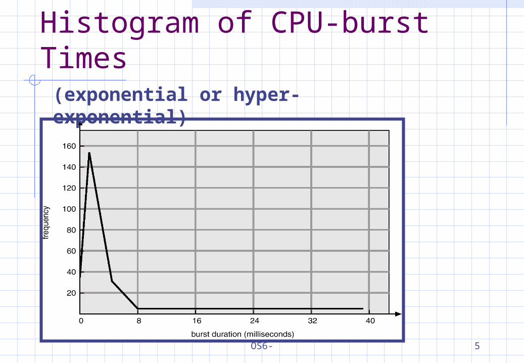
Histogram of CPU-burst Times(exponential or hyper-exponential)

OS6- 6

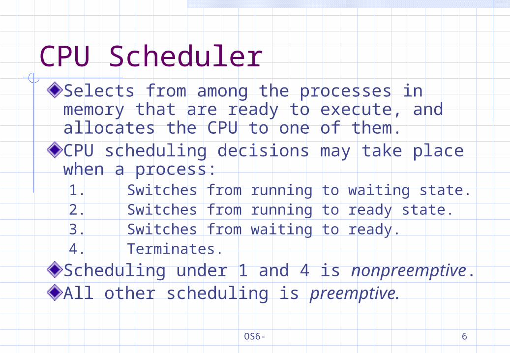
CPU SchedulerSelects from among the processes in memory that are ready to execute, and allocates the CPU to one of them.CPU scheduling decisions may take place when a process:1. Switches from running to waiting state.2. Switches from running to ready state.3. Switches from waiting to ready.4. Terminates.

Scheduling under 1 and 4 is nonpreemptive.All other scheduling is preemptive.

OS6- 7

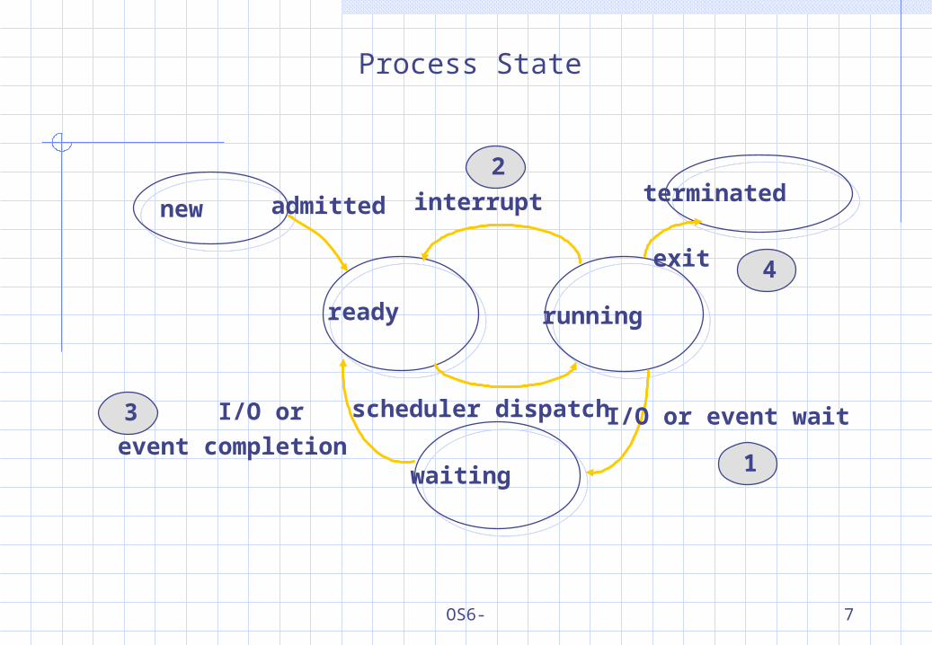
new

ready running

terminated

waiting

admitted interrupt

exit

scheduler dispatch I/O or event wait I/O or

event completion

Process State

1

4

3

2

OS6- 8

Dispatcher

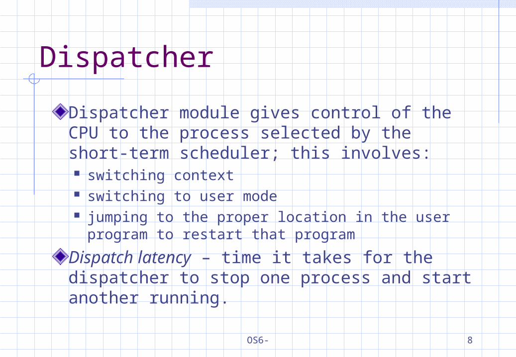
Dispatcher module gives control of the CPU to the process selected by the short-term scheduler; this involves: switching context switching to user mode jumping to the proper location in the user program

to restart that program

Dispatch latency – time it takes for the dispatcher to stop one process and start another running.

OS6- 9

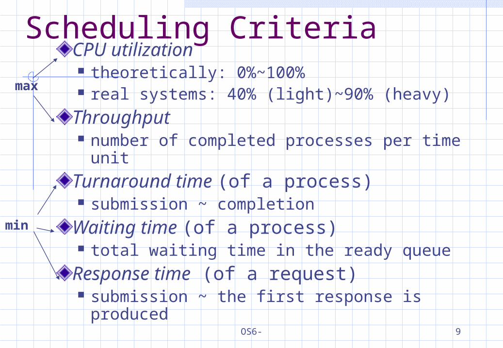
Scheduling CriteriaCPU utilization theoretically: 0%~100% real systems: 40% (light)~90% (heavy)

Throughput number of completed processes per time

unit

Turnaround time (of a process) submission ~ completion

Waiting time (of a process) total waiting time in the ready queue

Response time (of a request) submission ~ the first response is produced

max

min

OS6- 10

Optimization Criteria

Max CPU utilizationMax throughputMin turnaround time Min waiting time Min response time

OS6- 11

Scheduling Algorithmsfirst-come, first-served (FCFS) schedulingshortest-job-first (SJF) schedulingpriority schedulinground-robin schedulingmultilevel queue schedulingmultilevel feedback queue scheduling

OS6- 12

First-Come, First-Served Scheduling (1)

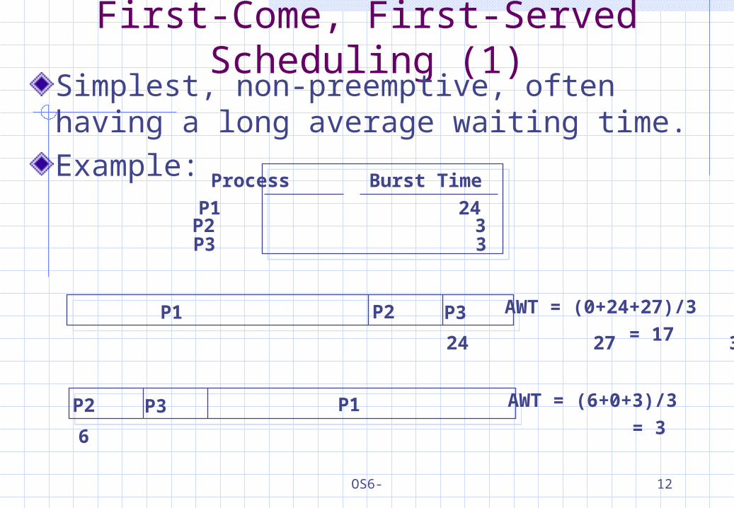
Simplest, non-preemptive, often having a long average waiting time.Example:

Process Burst Time

P1 24P2 3P3 3

P1 P2 P3

0 24 27 30

AWT = (0+24+27)/3

= 17

P1P2 P3

0 3 6 30

AWT = (6+0+3)/3

= 3

OS6- 13

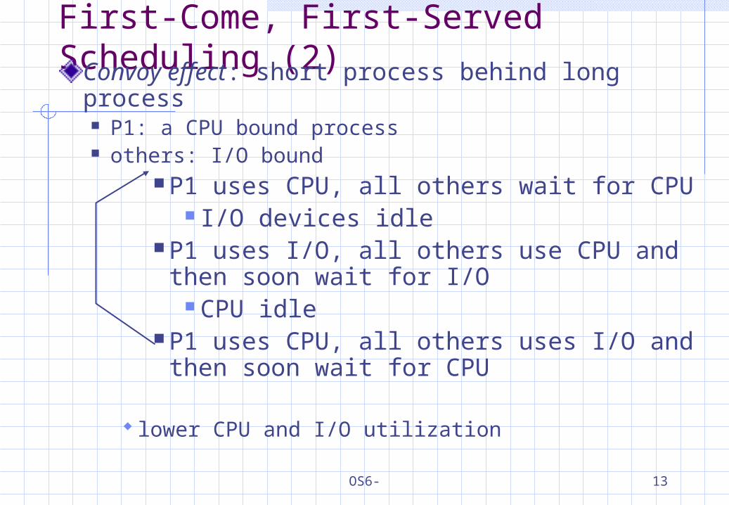
First-Come, First-Served Scheduling (2)Convoy effect: short process behind long

process P1: a CPU bound process others: I/O bound

P1 uses CPU, all others wait for CPU I/O devices idle

P1 uses I/O, all others use CPU and then soon wait for I/O

CPU idle P1 uses CPU, all others uses I/O and

then soon wait for CPU

lower CPU and I/O utilization

OS6- 14

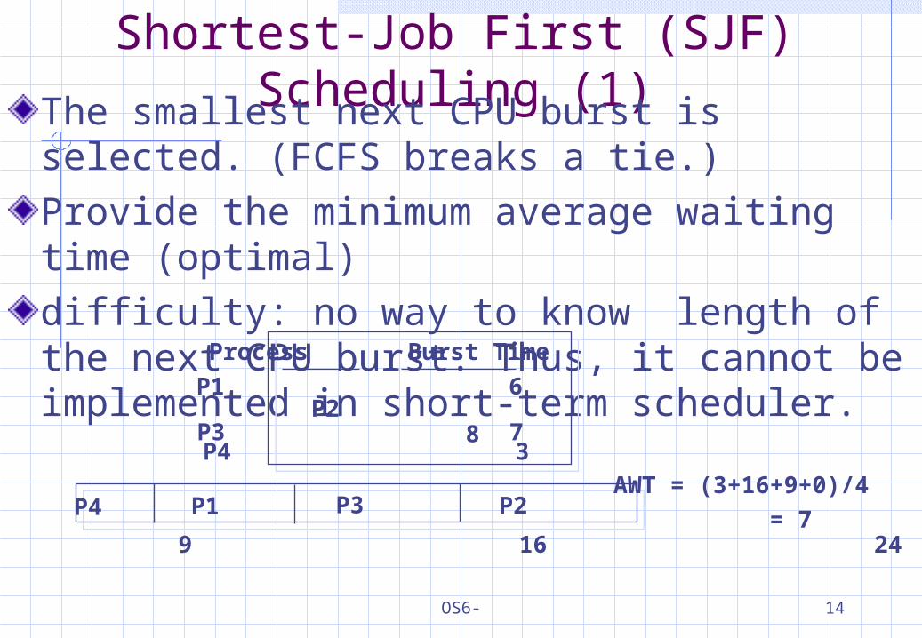
Shortest-Job First (SJF) Scheduling (1)The smallest next CPU burst is selected.

(FCFS breaks a tie.)Provide the minimum average waiting time (optimal)difficulty: no way to know length of the next CPU burst. Thus, it cannot be implemented in short-term scheduler.

P1 P2P3

0 3 9 16 24

Process Burst Time

P1 6P2

8P3 7 P4 3

P4AWT = (3+16+9+0)/4

= 7

OS6- 15

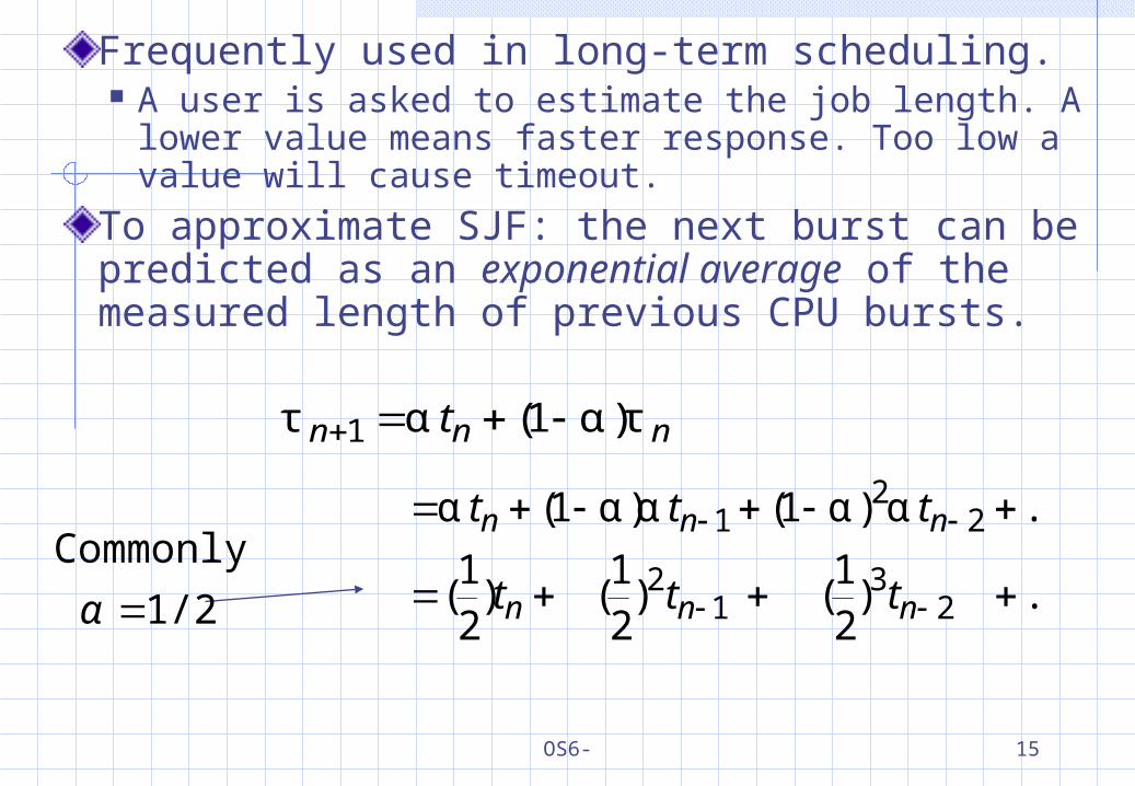
Frequently used in long-term scheduling. A user is asked to estimate the job length. A

lower value means faster response. Too low a value will cause timeout.

To approximate SJF: the next burst can be predicted as an exponential average of the measured length of previous CPU bursts.

nnn t τ)α1(ατ 1

... )21

( )21

( )21

(

...α)α1(α)α1(α

23

12

22

1

nnn

nnn

ttt

ttt

1/2

Commonly,

α

OS6- 16

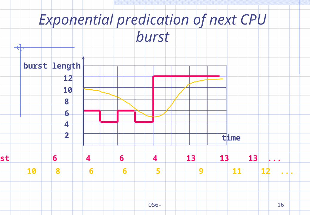
Exponential predication of next CPU burst

24681012

burst length

time

CPU burst 6 4 6 4 13 13 13 ...

guess 10 8 6 6 5 9 11 12 ...

OS6- 17

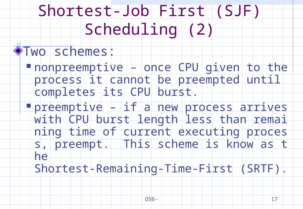
Shortest-Job First (SJF) Scheduling (2)

Two schemes: nonpreemptive – once CPU given to the pr

ocess it cannot be preempted until completes its CPU burst.

preemptive – if a new process arrives with CPU burst length less than remaining time of current executing process, preempt. This scheme is know as the Shortest-Remaining-Time-First (SRTF).

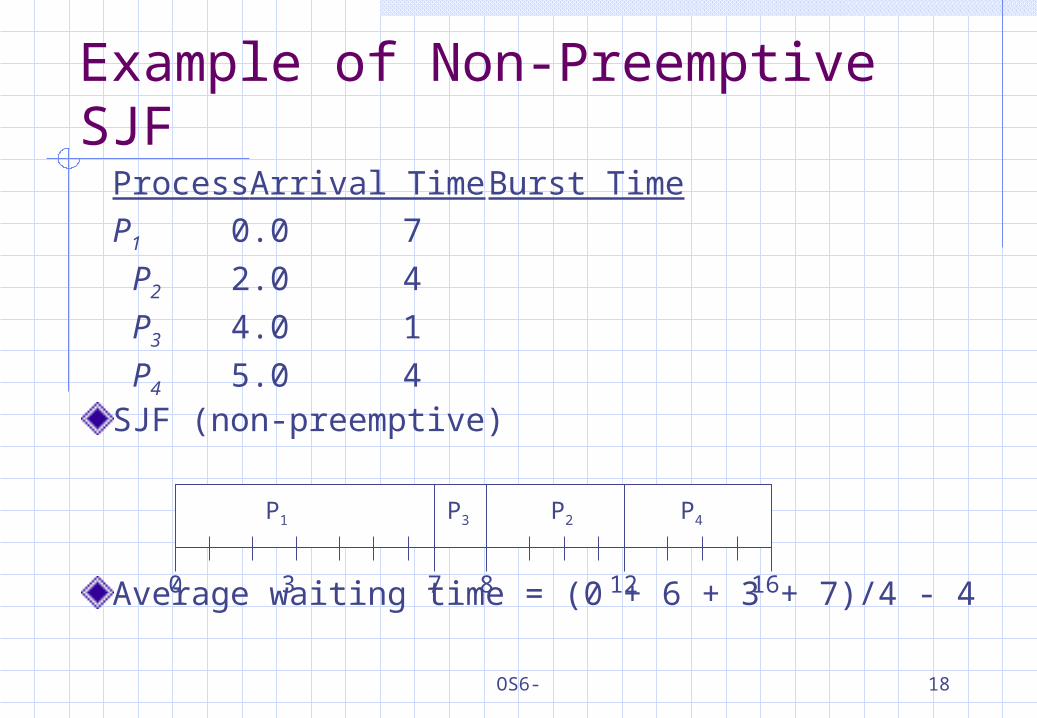
OS6- 18

ProcessArrival TimeBurst TimeP1 0.0 7

P2 2.0 4

P3 4.0 1

P4 5.0 4SJF (non-preemptive)

Average waiting time = (0 + 6 + 3 + 7)/4 - 4

Example of Non-Preemptive SJF

P1 P3 P2

73 160

P4

8 12

OS6- 19

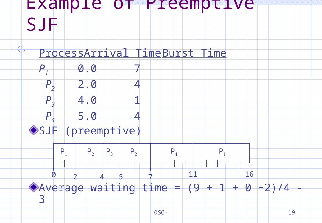
Example of Preemptive SJF

ProcessArrival TimeBurst TimeP1 0.0 7

P2 2.0 4

P3 4.0 1

P4 5.0 4SJF (preemptive)

Average waiting time = (9 + 1 + 0 +2)/4 - 3

P1 P3P2

42 110

P4

5 7

P2 P1

16

OS6- 20

Priority SchedulingA priority number (integer) is associated with each processThe CPU is allocated to the process with the highest priority (smallest integer highest priority). Preemptive nonpreemptive

SJF is a priority scheduling where priority is the predicted next CPU burst time.Problem Starvation – low priority processes may never execute. (At MIT, there was a job submitted in 1967 that had not be run in 1973.)

Solution Aging – as time progresses increase the priority of the process.

OS6- 21

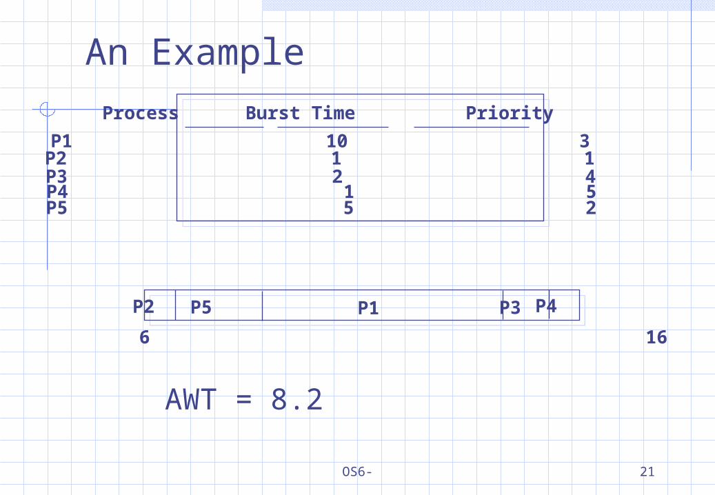
Process Burst Time Priority

P1 10 3P2 1 1P3 2 4P4 1 5

P5 P3

0 1 6 16 18 19P4P2 P1

P5 5 2

AWT = 8.2

An Example

OS6- 22

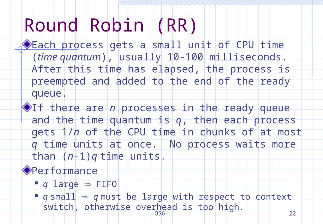
Round Robin (RR)Each process gets a small unit of CPU time (time quantum), usually 10-100 milliseconds. After this time has elapsed, the process is preempted and added to the end of the ready queue.If there are n processes in the ready queue and the time quantum is q, then each process gets 1/n of the CPU time in chunks of at most q time units at once. No process waits more than (n-1)q time units.Performance q large FIFO q small q must be large with respect to context

switch, otherwise overhead is too high.

OS6- 23

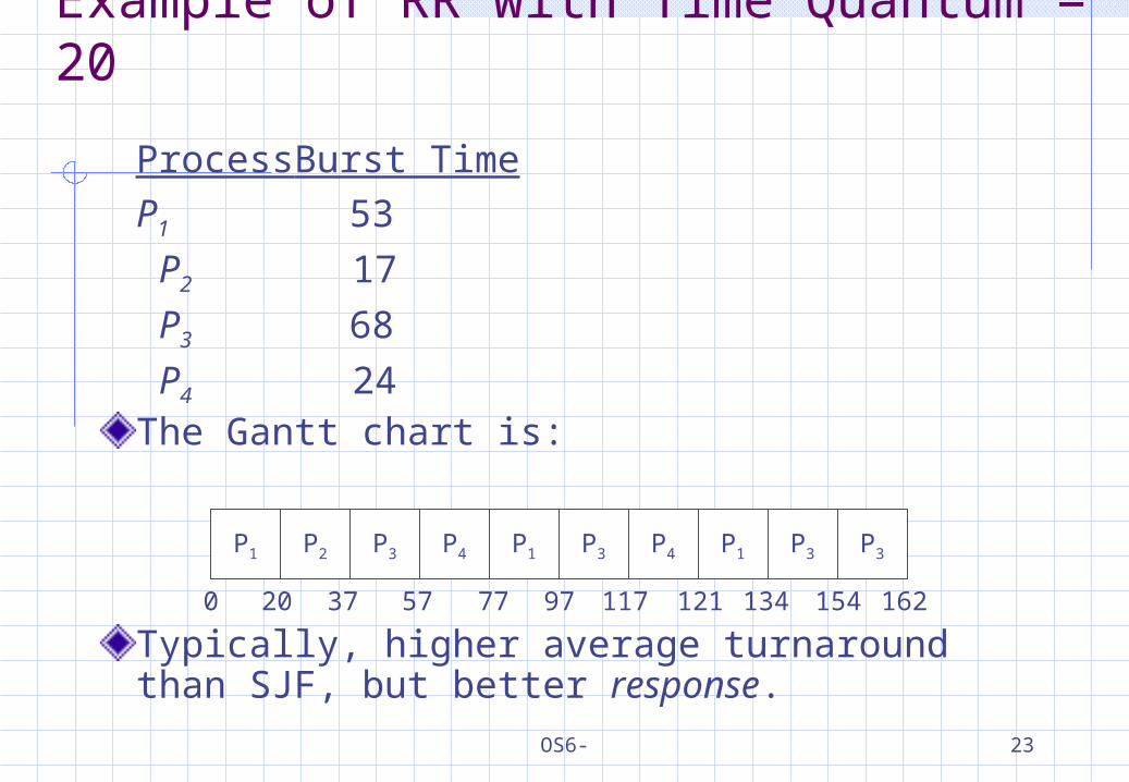
Example of RR with Time Quantum = 20

Process Burst TimeP1 53

P2 17

P3 68

P4 24The Gantt chart is:

Typically, higher average turnaround than SJF, but better response.

P1 P2 P3 P4 P1 P3 P4 P1 P3 P3

0 20 37 57 77 97 117 121 134 154 162

OS6- 24

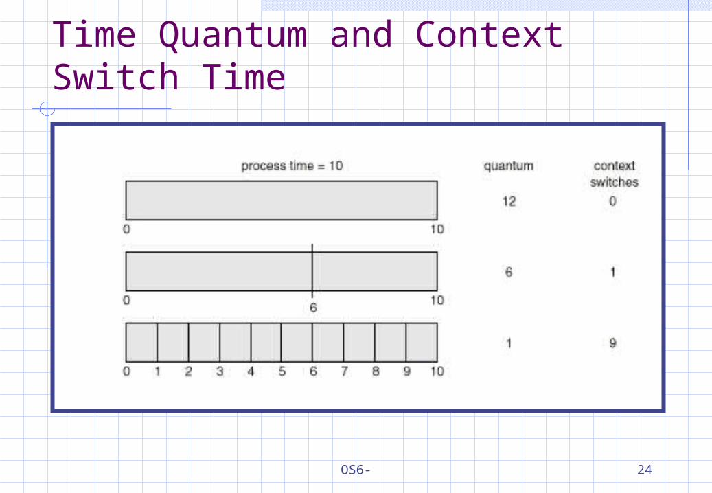
Time Quantum and Context Switch Time

OS6- 25

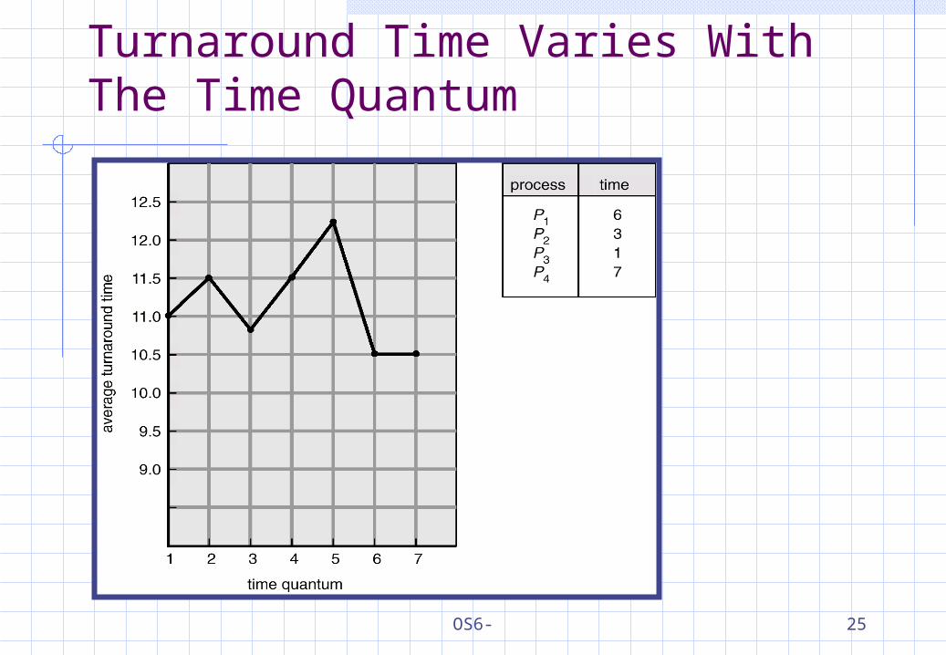
Turnaround Time Varies With The Time Quantum

OS6- 26

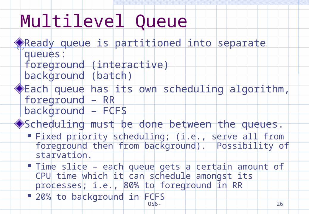
Multilevel QueueReady queue is partitioned into separate queues:foreground (interactive)background (batch)Each queue has its own scheduling algorithm, foreground – RRbackground – FCFSScheduling must be done between the queues. Fixed priority scheduling; (i.e., serve all from foreground

then from background). Possibility of starvation. Time slice – each queue gets a certain amount of CPU

time which it can schedule amongst its processes; i.e., 80% to foreground in RR

20% to background in FCFS

OS6- 27

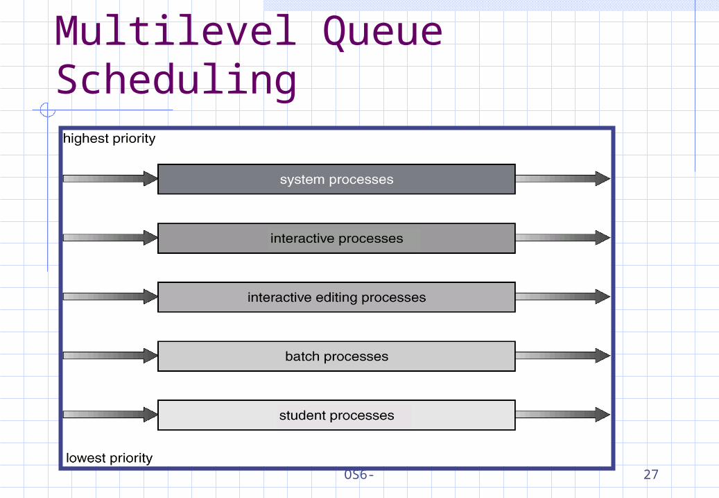
Multilevel Queue Scheduling

OS6- 28

Multilevel Feedback QueueA process can move between the various queues; aging can be implemented this way.Multilevel-feedback-queue scheduler defined by the following parameters: number of queues scheduling algorithms for each queue method used to determine when to upgrade a

process method used to determine when to demote a

process method used to determine which queue a process

will enter when that process needs service

OS6- 29

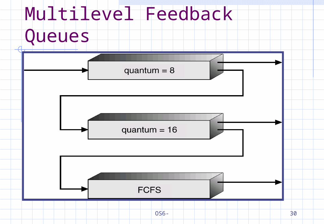
Example of Multilevel Feedback Queue

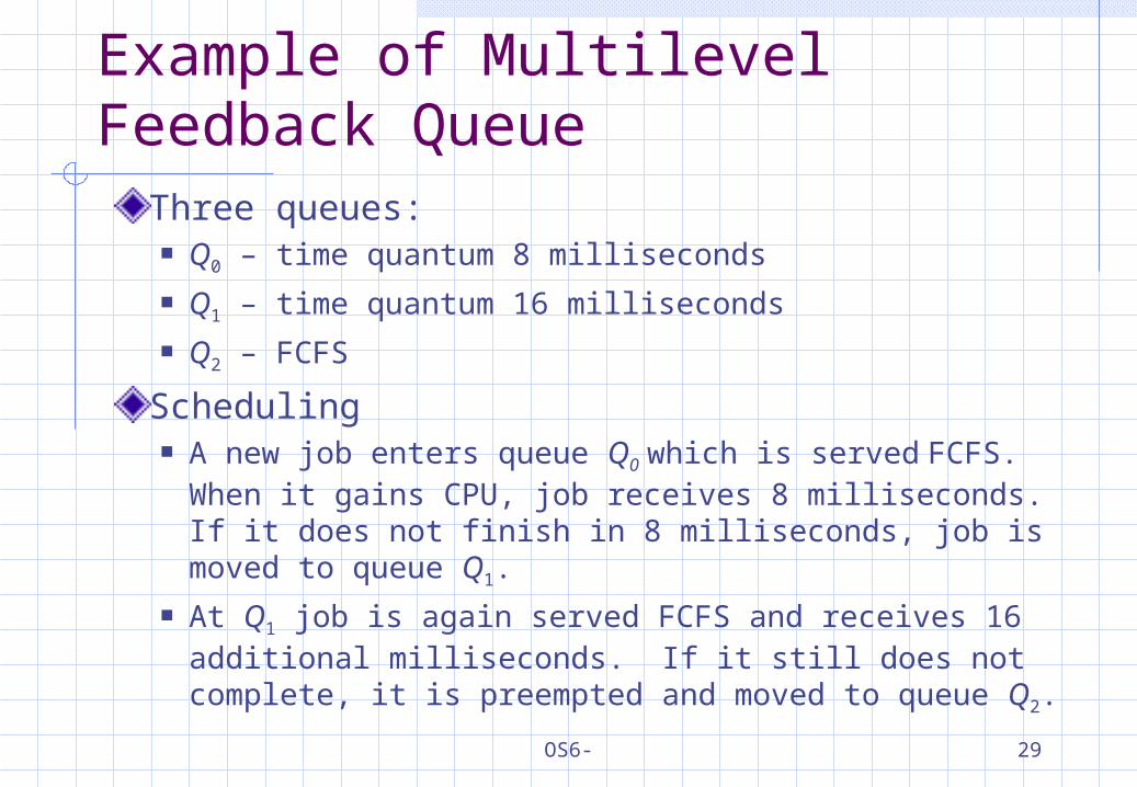
Three queues: Q0 – time quantum 8 milliseconds Q1 – time quantum 16 milliseconds Q2 – FCFS

Scheduling A new job enters queue Q0 which is served FCFS. When

it gains CPU, job receives 8 milliseconds. If it does not finish in 8 milliseconds, job is moved to queue Q1.

At Q1 job is again served FCFS and receives 16 additional milliseconds. If it still does not complete, it is preempted and moved to queue Q2.

OS6- 30

Multilevel Feedback Queues

OS6- 31

Multiple-Processor SchedulingHere, only homogeneous systems are discussed hereScheduling1. Each processor has a separate queue2. All process use a common ready queue

a. Each processor is self-schedulingb. Appoint a processor as scheduler for the other processes (the master-slave structure).

Load sharing Asymmetric multiprocessing: all system activities are handled by a processor, the others only execute user code (allocated by the master), which is far simple than symmetric multiprocessing

OS6- 32

Real-Time Scheduling (1)

Hard real-time systems – required to complete a critical task within a guaranteed amount of time. Resource reservation is needed. special purpose software on dedicated HW

Soft real-time computing – requires that critical processes receive priority over less fortunate ones.

OS6- 33

Real-Time Scheduling (2)Scheduler for soft real-time system Priority scheduling (real-time process must have the

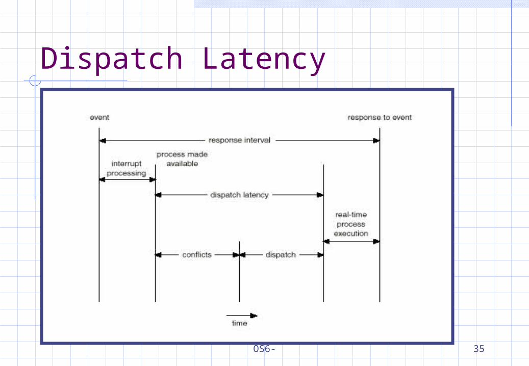
highest priority). Easy! The dispatch latency must be small.

Problem: Most OS waits a system call to complete (or I/O block to take place) before doing context switch.

Solution: system calls should be pre-emptible.

Insert preemption points in long-duration system calls. (The latency is still long. There are a few preemption points).

Make the entire kernel preemptible.

OS6- 34

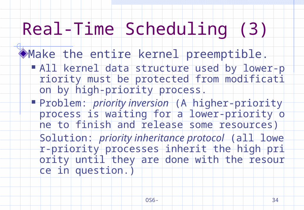
Real-Time Scheduling (3)Make the entire kernel preemptible. All kernel data structure used by lower-priority

must be protected from modification by high-priority process.

Problem: priority inversion (A higher-priority process is waiting for a lower-priority one to finish and release some resources)Solution: priority inheritance protocol (all lower-priority processes inherit the high priority until they are done with the resource in question.)

OS6- 35

Dispatch Latency

OS6- 36

Algorithm EvaluationCriteria to select a CPU scheduling algorithm may include several measures, such as : Maximize CPU utilization under the constraint

that the maximum response time is 1 second Maximize throughput such that turnaround time

is (on average) linearly proportional to total execution time

Evaluation methods ? deterministic modeling queuing models simulations implementation

OS6- 37

Deterministic modeling (1)

Analytic evaluation:Input: a given algorithm and a system

workload to Output: performance of the algorithm for

that workload

Deterministic modeling: Taking a particular predetermined

workload and defining the performance of each algorithm for that workload.

OS6- 38

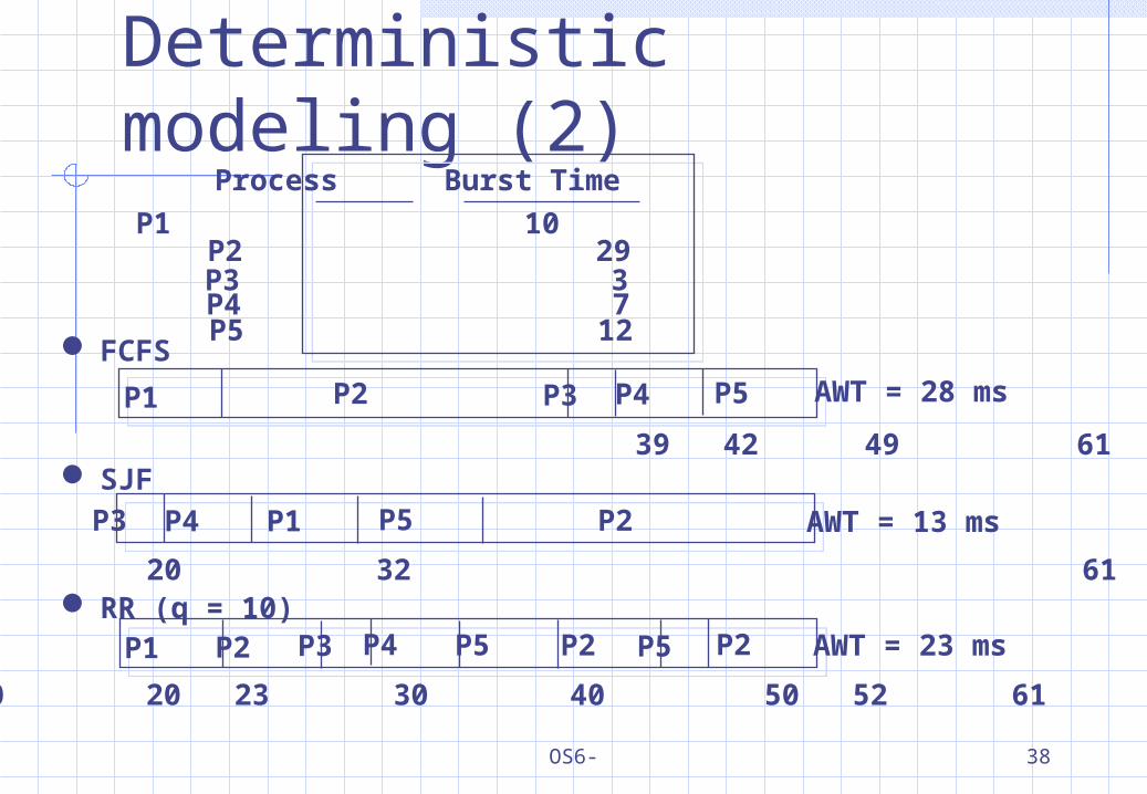
Deterministic modeling (2)

FCFS

SJF

RR (q = 10)

Process Burst Time

P1 10 P2 29P3 3P4 7

P5P3

0 10 39 42 49 61P4P2P1

P5 12

P5P3

0 3 10 20 32 61P4 P2P1

P5P3

0 10 20 23 30 40 50 52 61P4P2P1 P2 P2P5

AWT = 28 ms

AWT = 13 ms

AWT = 23 ms

OS6- 39

Deterministic modeling (3)

: A simple and fast method. It gives the exact numbers, allows the algorithms to be compared.

: It requires exact numbers of input, and its answers apply to only those cases. In general, deterministic modeling is too specific, and requires too much exact knowledge, to be useful.Usage Describing algorithm and providing examples. A set of programs that may run over and over again. Indicating the trends that can then be proved.

OS6- 40

Queuing Models (1)Queuing network analysis Using

the distribution of service times (CPU and I/O bursts)

the distribution of process arrival times The computer system is described as a

network of servers. Each server has a queue of waiting processes.

Determining utilization, average queue length, average waiting

time, and so on.

OS6- 41

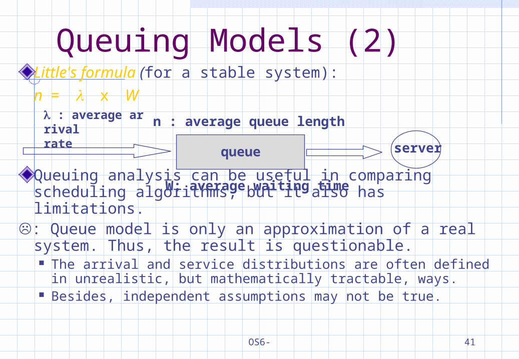
Queuing Models (2)Little's formula (for a stable system):

n = x W

Queuing analysis can be useful in comparing scheduling algorithms, but it also has limitations.

: Queue model is only an approximation of a real system. Thus, the result is questionable. The arrival and service distributions are often defined in

unrealistic, but mathematically tractable, ways. Besides, independent assumptions may not be true.

n : average queue length

W: average waiting time

queue server

: average arrival rate

OS6- 42

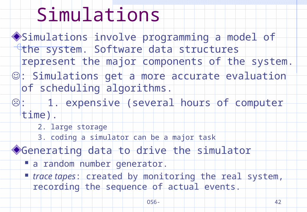
SimulationsSimulations involve programming a model of the system. Software data structures represent the major components of the system.

: Simulations get a more accurate evaluation of scheduling algorithms.

: 1. expensive (several hours of computer time).

2. large storage3. coding a simulator can be a major task

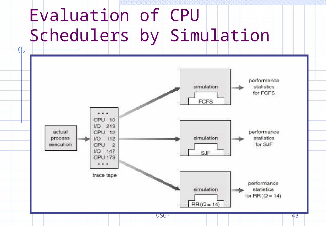
Generating data to drive the simulator a random number generator. trace tapes: created by monitoring the real system,

recording the sequence of actual events.

OS6- 43

Evaluation of CPU Schedulers by Simulation

OS6- 44

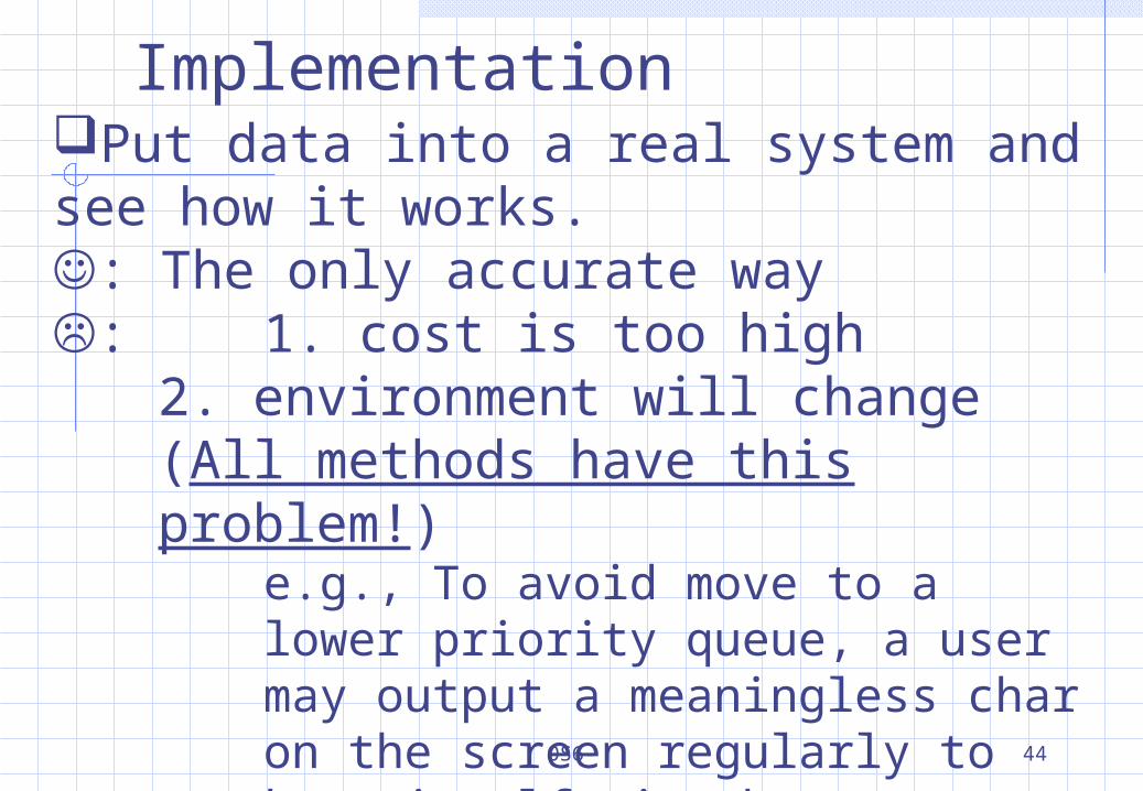
ImplementationPut data into a real system and see how it works.: The only accurate way: 1. cost is too high

2. environment will change (All methods have this problem!)

e.g., To avoid move to a lower priority queue, a user may output a meaningless char on the screen regularly to keep itself in the interactive queue.

OS6- 45

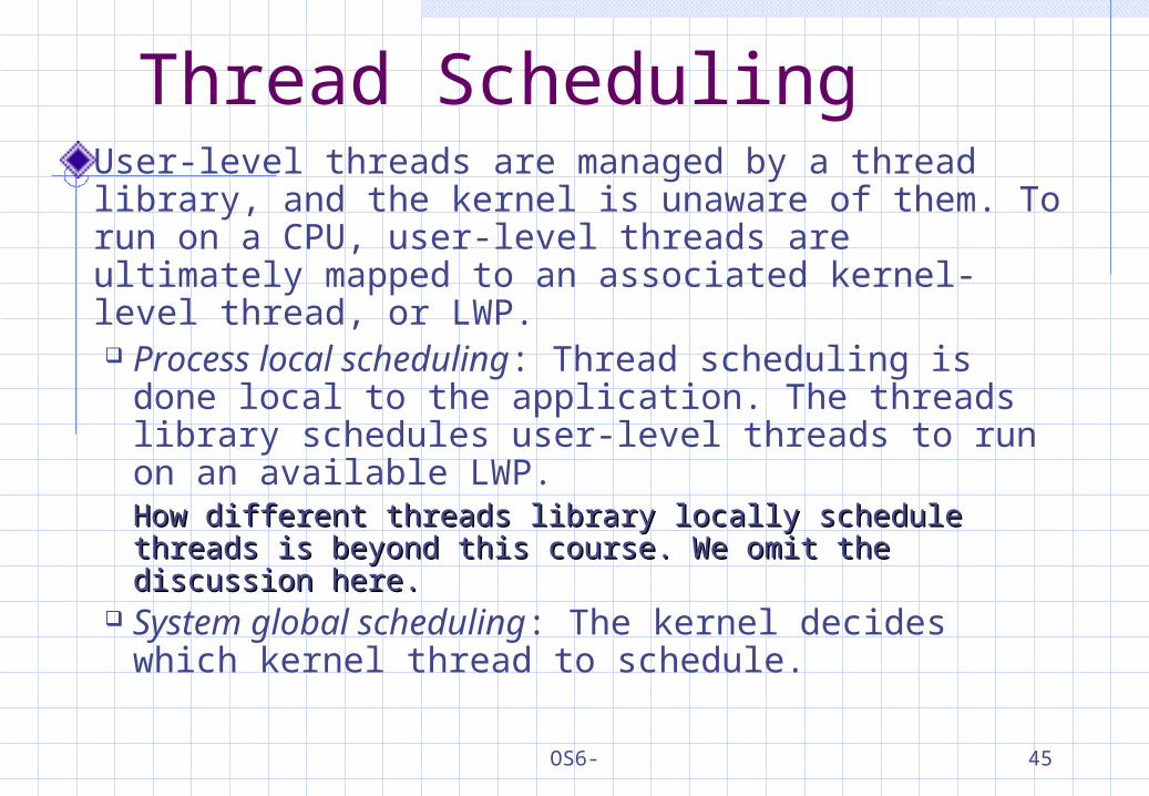
Thread SchedulingUser-level threads are managed by a thread library, and the kernel is unaware of them. To run on a CPU, user-level threads are ultimately mapped to an associated kernel-level thread, or LWP. Process local scheduling: Thread scheduling is

done local to the application. The threads library schedules user-level threads to run on an available LWP.How different threads library locally schedule threads How different threads library locally schedule threads is beyond this course. We omit the discussion here.is beyond this course. We omit the discussion here.

System global scheduling: The kernel decides which kernel thread to schedule.

OS6- 46

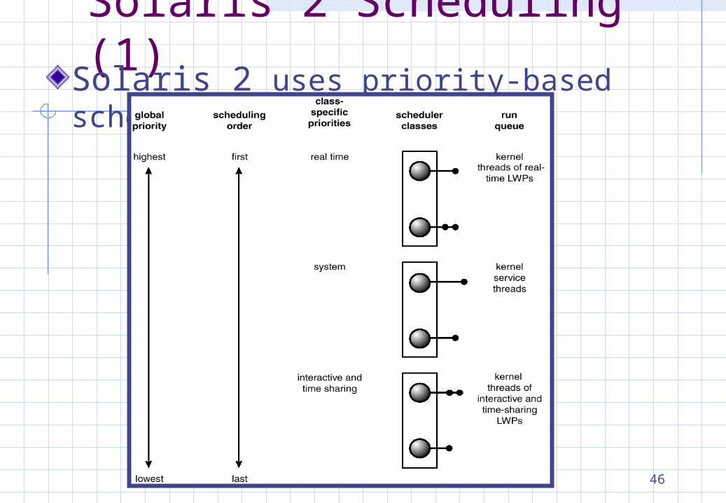
Solaris 2 Scheduling (1)Solaris 2 uses priority-based scheduling.

OS6- 47

Solaris 2 Scheduling (2)Four classes of scheduling: real-time -> system -> time sharing -> scheduling.A process starts with one LWP and is able to create new LWPs as needed. Each LWP inherits the scheduling class and priority of the parent process. Default : time sharing (multilevel feedback queue)Inverse relationship between priorities and time slices: the high the priority, the smaller the time slice.Interactive processes typical have a higher priority; CPU-bound processes a lower priority.

OS6- 48

Solaris 2 Scheduling (3)

Uses the system class to run kernel processes, such as the scheduler and page daemon. The system class is reserved for kernel use only.Threads in the real-time class are given the highest priority to run among all classes. There is a set of priorities within each class. However, the scheduler converts the class-specific priorities into global priorities. (round-robin queue)

OS6- 49

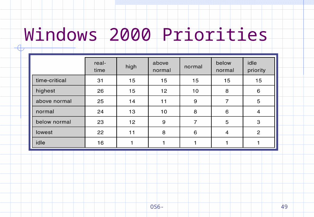
Windows 2000 Priorities

OS6- 50

Java Thread Scheduling (1)

Preemptive, priority-based scheduling (FIFO queue)Time slicing: Java does not indicate whether or not

threads are time-sliced or not – it is up to the particular implementation of the JVM.

All threads have an equal amount of CPU time on a system that does not perform time slicing, a thread may yield control of the CPU with the yield() method. Cooperative multitasking.

Thread.yield();

OS6- 51

Java Thread Scheduling (2)

Thread priorities: Threads are given a priority when they are create

d and – unless they are changed explicitly by the program – they maintain the same priority throughout their lifetime; the JVM does not dynamically alter priorities.

The priority of a thread can also be set explicitly with the setPriority() method. The priority can be set either before a thread is started or while a thread is active.

Java-Based Round-robin Scheduler