Oswietlenie i cieniowanie´ - wmii.uwm.edu.plwmii.uwm.edu.pl/~denisjuk/uwm/3d/wyklady/04-oswietlenie.pdf · Modelowanie i wizualizowanie 3W-graﬁki Oswietlenie i cieniowanie´ Aleksander

Modelowanie i wizualizowanie 3W-grafiki

Oswietlenie i cieniowanie

Aleksander Denisiuk

[email protected]

Uniwersytet Warminsko-Mazurski w Olsztynie

Wydział Matematyki i Informatyki

ul. Słoneczna 54

10-561 Olsztyn

Modelowanie i wizualizowanie 3W-grafiki – p. 1

Oswietlenie i cieniowanie

Najnowsza wersja tego dokumentu dostepna jest podadresem http://wmii.uwm.edu.pl/~denisjuk/uwm


http://wmii.uwm.edu.pl/~denisjuk/uwm

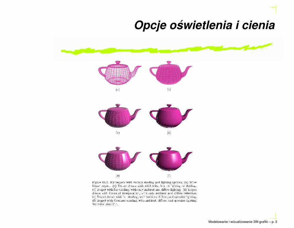
Opcje oswietlenia i cienia

(a) (b)

( ) (d)

(e) (f)

Figure III.1: Six teapots with various shading and lighting options. (a) Wire-

frame teapot. (b) Teapot drawn with solid olor, but no lighting or shading.

( ) Teapot with at shading, with only ambient and di�use lighting. (d) Teapot

drawn with Gouraud interpolation, with only ambient and di�use re e tion.

(e) Teapot drawn with at shading, with ambient, di�use, and spe ular lighting.

(f) Teapot with Gouraud shading, with ambient, di�use, and spe ular lighting.

See olor plate C.4.


Oswietlenie Phonga

Model odbicia swiatła

Zródło swiatła — punkt

Swiatło ma trzy składowe, RGB


Odbicie rozproszone

zabarwia swiatło na kolor przypisany do obiektu.

Light sour e

Figure III.2: Di�usely re e ted light is re e ted equally brightly in all dire tions.

The double line is a beam of in oming light. The dotted arrows indi ate outgoing

light.


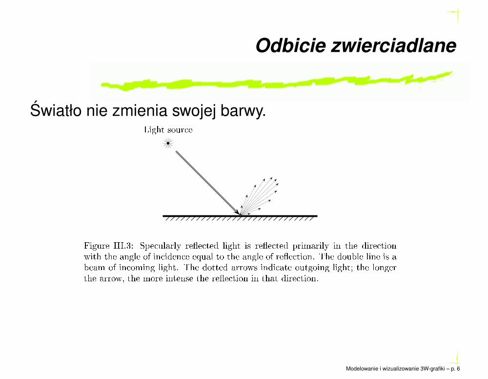
Odbicie zwierciadlane

Swiatło nie zmienia swojej barwy.

Light sour e

Figure III.3: Spe ularly re e ted light is re e ted primarily in the dire tion

with the angle of in iden e equal to the angle of re e tion. The double line is a

beam of in oming light. The dotted arrows indi ate outgoing light; the longer

the arrow, the more intense the re e tion in that dire tion.


Swiatło docierajace do obserwatora

Swiatło odbijane zwierciadlane: Is.

Swiatło rozproszone: Id.

Swiatło otoczenia: Ia.

Swiatło emitowane powierzchnia: Ie.

I = Is + Id + Ia + Ie


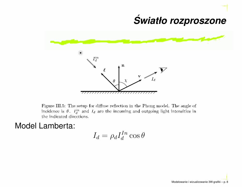
Swiatło rozproszone

`

n

v

�

�

I

in

d

I

d

Figure III.5: The setup for di�use re e tion in the Phong model. The angle of

in iden e is � . I

in

d

and I

d

are the in oming and outgoing light intensities in

the indi ated dire tions.

Model Lamberta:Id = ρdI

Ind cos θ


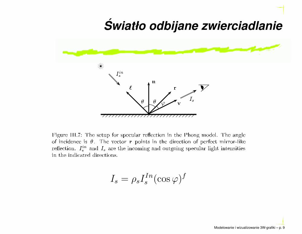
Swiatło odbijane zwierciadlanie

` r

n

v

� �

'

I

in

s

I

s

Figure III.7: The setup for spe ular re e tion in the Phong model. The angle

of in iden e is � . The ve tor r points in the dire tion of perfe t mirror-like

re e tion. I

in

s

and I

s

are the in oming and outgoing spe ular light intensities

in the indi ated dire tions.

Is = ρsIIns (cosϕ)f


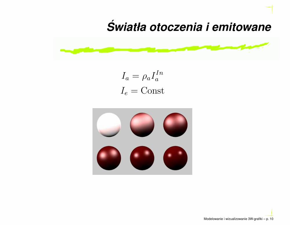
Swiatła otoczenia i emitowane

Ia = ρaIIna

Ie = Const


Obliczanie wektora normalgego

trójkat

powierzchnia parametryzowana

powierzchnia okreslona równaniem


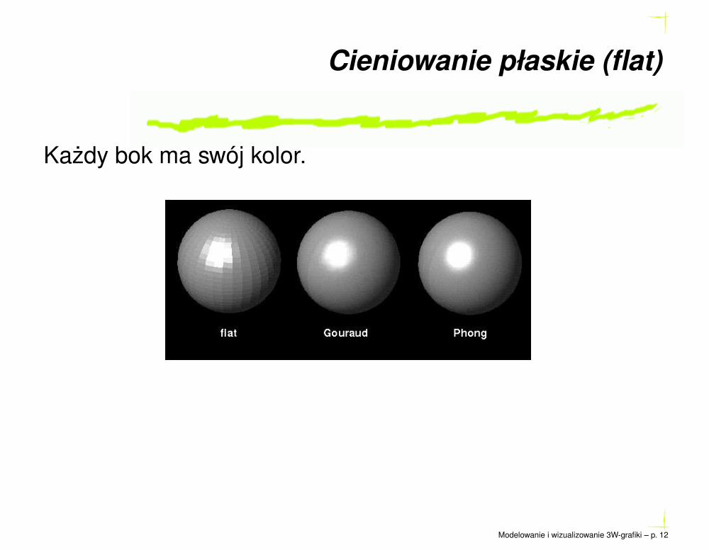
Cieniowanie płaskie (flat)

Kazdy bok ma swój kolor.


Cieniowanie Gourauda

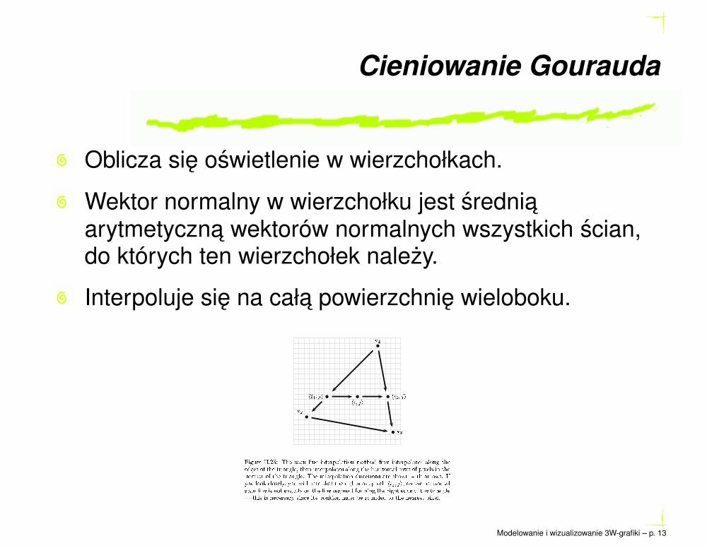
Oblicza sie oswietlenie w wierzchołkach.

Wektor normalny w wierzchołku jest sredniaarytmetyczna wektorów normalnych wszystkich scian,do których ten wierzchołek nalezy.

Interpoluje sie na cała powierzchnie wieloboku.v

1

v

2

v

3

hi; ji

hi

4

; ji hi

5

; ji

Figure II.25: The s an line interpolation method �rst interpolates along the

edges of the triangle, then interpolates along the horizontal rows of pixels in the

interior of the triangle. The interpolation dire tions are shown with arrows. If

you look losely, you will note that the rightmost pixel, hi

5

; ji , on the horizontal

s an line is not exa tly on the line segment forming the right edge of the triangle

| this is ne essary sin e its position must be rounded to the nearest pixel.



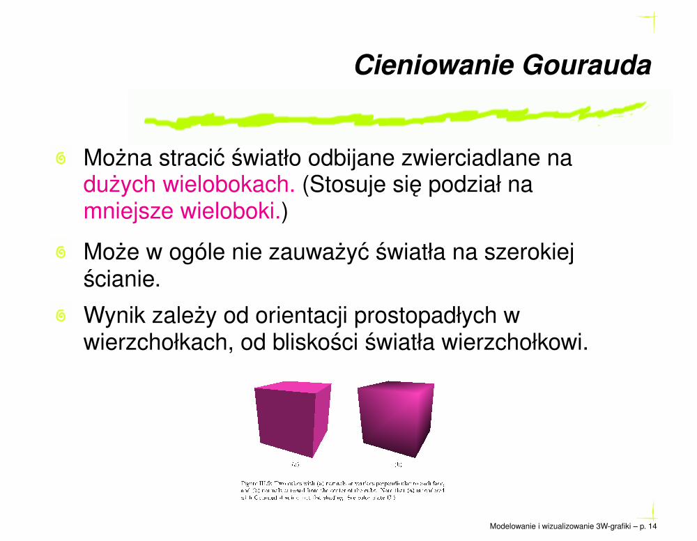
Mozna stracic swiatło odbijane zwierciadlane naduzych wielobokach. (Stosuje sie podział namniejsze wieloboki.)

Moze w ogóle nie zauwazyc swiatła na szerokiejscianie.

Wynik zalezy od orientacji prostopadłych wwierzchołkach, od bliskosci swiatła wierzchołkowi.

(a) (b)

Figure III.9: Two ubes with (a) normals at verti es perpendi ular to ea h fa e,

and (b) normals outward from the enter of the ube. Note that (a) is rendered

with Gouraud shading, not at shading. See olor plate C.5.


Gouraud_low_anim.gif

Gouraud_high.gif


Dobrze działa w wielu przypadkach.

Łatwo do implementacji zarówno programowej jaki sprzetowej.

Jest rozpowszechnione.


Cieniowanie Phonga

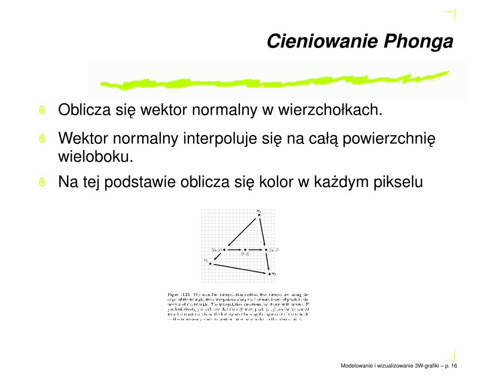
Oblicza sie wektor normalny w wierzchołkach.

Wektor normalny interpoluje sie na cała powierzchniewieloboku.

Na tej podstawie oblicza sie kolor w kazdym pikselu

v

1

v

2

v

3

hi; ji

hi

4

; ji hi

5

; ji

Figure II.25: The s an line interpolation method �rst interpolates along the

edges of the triangle, then interpolates along the horizontal rows of pixels in the

interior of the triangle. The interpolation dire tions are shown with arrows. If

you look losely, you will note that the rightmost pixel, hi

5

; ji , on the horizontal

s an line is not exa tly on the line segment forming the right edge of the triangle

| this is ne essary sin e its position must be rounded to the nearest pixel.


Cieniowanie Phonga

Kosztowne obliczenia: nα = αn1+(1−α)n0

‖αn1+(1−α)n0‖.

Cała informacja o kolorach i kierunkach swiatłapowinna przechowywac sie do ostatniej stadji obliczen.

Interpolacja we współrzednych ekranowych: mogawystapic nieporzadane efekty przy projekcjiperspektywicznej.


Cieniowanie Phonga

Małe odbicia zwierciadlane sie nie gubia na duzychwielobokach.


Obserwator lokany i nielokalny

` r

h

n

v

�

'

I

in

s

I

s

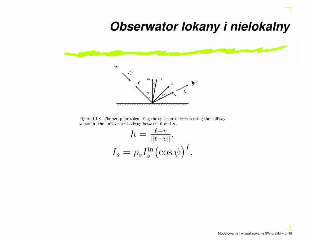
Figure III.8: The setup for al ulating the spe ular re e tion using the halfway

ve tor h , the unit ve tor halfway between ` and v .

h = ℓ+v‖ℓ+v‖

,

Is = ρsIins

(

cosψ)f.


Normalizacja wektorów

Domyslnie kazdy wektor jednostkowy powinien bycnormalizowany.

Jezeli macierz przekształcenia zawiera skalowanie,wektory nalezy normalizowac.


BRIDF

`

n

v

I

�;in

I

�;out

Figure III.13: The BRIDF fun tion relates the outgoing light intensity and the

in oming light intensity a ording to BRIDF(` ;v; �) = I

�;out

=I

�;in

:

Funkcja rozkładu współczynnika odbicia dwukierunkowego(Bidirectional Reflected Intesity Distridution Function)


Powierzchnia mikroluster

I

1

I

2

Figure III.14: A mi rofa et surfa e onsists of small at pie es. The horizontal

line shows the average level of a at surfa e, and the mi rofa ets show the

mi ros opi shape of the surfa e. Dotted lines show the dire tion of light rays.

The in oming light an either be re e ted in the dire tion of perfe t mirror-like

re e tion (I

1

), or an enter the surfa e (I

2

). In the se ond ase, the light is

modeled as eventually exiting the material as di�usely re e ted light.


Model Cooka-Torrance’a (1982)

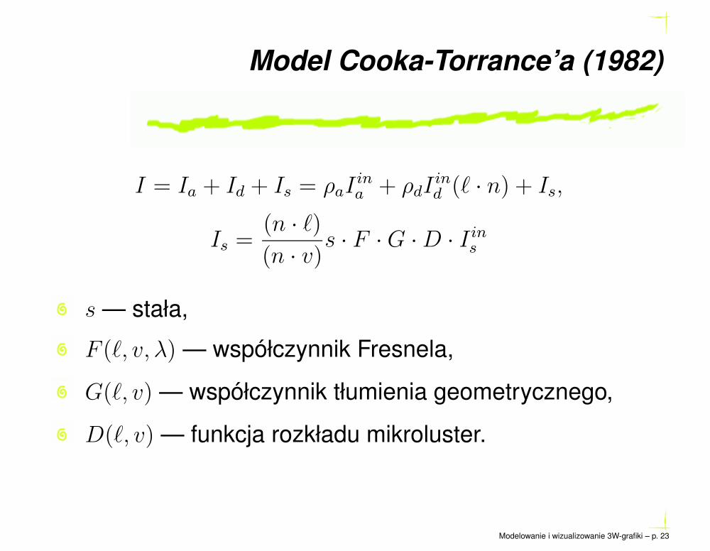
I = Ia + Id + Is = ρaIina + ρdI

ind (ℓ · n) + Is,

Is =(n · ℓ)

(n · v)s · F ·G ·D · I ins

s — stała,

F (ℓ, v, λ) — współczynnik Fresnela,

G(ℓ, v) — współczynnik tłumienia geometrycznego,

D(ℓ, v) — funkcja rozkładu mikroluster.


Funkcja Rozkładu Mikroluster

` r

h

n

v

�

'

I

in

s

I

s

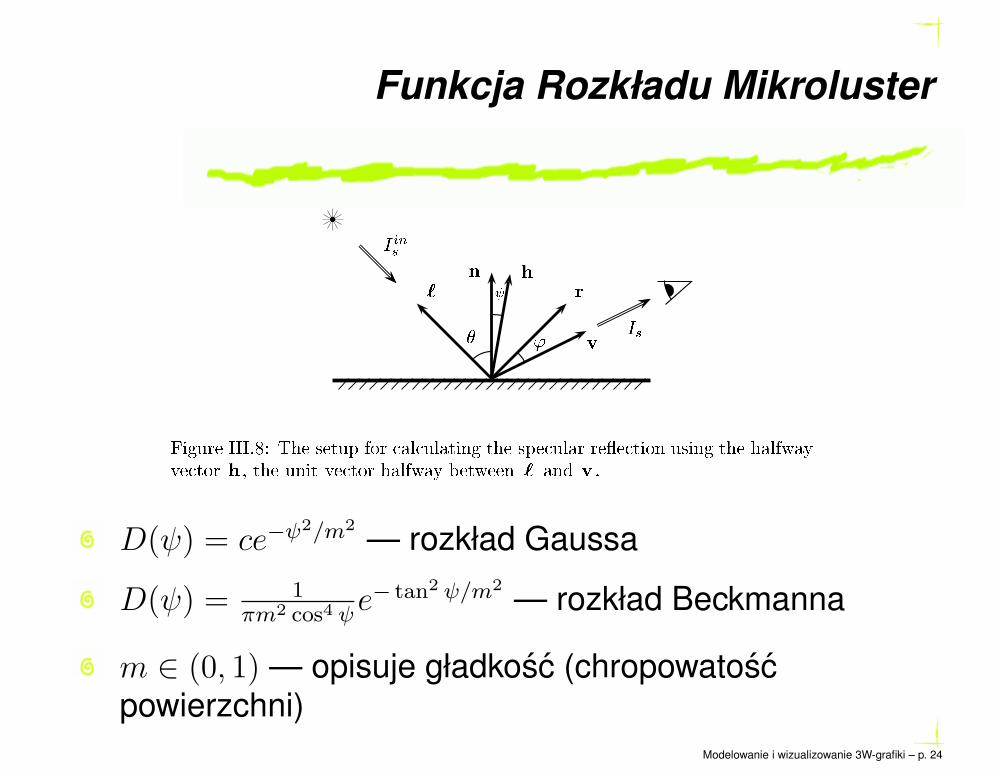
Figure III.8: The setup for al ulating the spe ular re e tion using the halfway

ve tor h , the unit ve tor halfway between ` and v .

D(ψ) = ce−ψ2/m2

— rozkład Gaussa

D(ψ) = 1πm2 cos4 ψ

e− tan2 ψ/m2

— rozkład Beckmanna

m ∈ (0, 1) — opisuje gładkosc (chropowatoscpowierzchni)


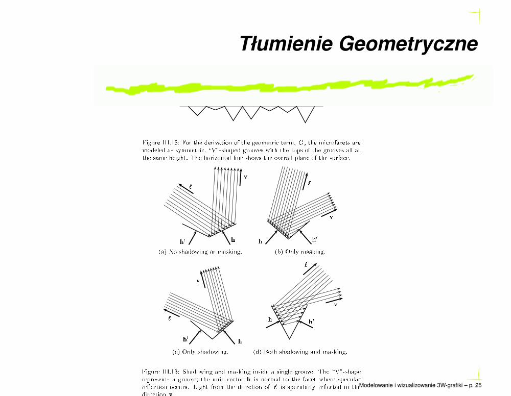
Tłumienie Geometryczne

Figure III.15: For the derivation of the geometri term, G , the mi rofa ets are

modeled as symmetri , \V"-shaped grooves with the tops of the grooves all at

the same height. The horizontal line shows the overall plane of the surfa e.

h

0 h

`

v

h

h

0

`

v

(a) No shadowing or masking. (b) Only masking.

h

h

0

v

`

h

h

0

`

v

( ) Only shadowing. (d) Both shadowing and masking.

Figure III.16: Shadowing and masking inside a single groove. The \V"-shape

represents a groove; the unit ve tor h is normal to the fa et where spe ular

re e tion o urs. Light from the dire tion of ` is spe ularly re e ted in the

dire tion v .


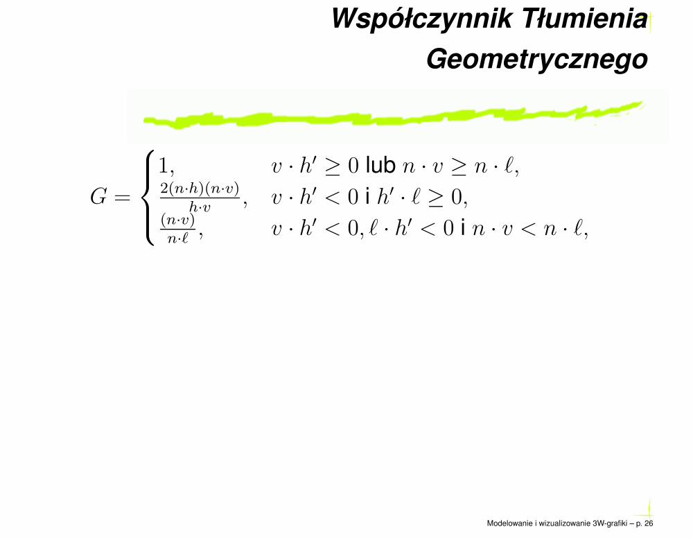
Współczynnik Tłumienia

Geometrycznego

G =

1, v · h′ ≥ 0 lub n · v ≥ n · ℓ,2(n·h)(n·v)

h·v, v · h′ < 0 i h′ · ℓ ≥ 0,

(n·v)n·ℓ

, v · h′ < 0, ℓ · h′ < 0 i n · v < n · ℓ,


Współczynnik Fresnela

F ≈ F0 + (1− F0)(1− cosψ)5

Tabela 1: Wartosci F0 dla wybranych materiałówR G B

Złoto: 0,93 0,88 0,38

Srebro: 0,97 0,97 0,96

Platyna: 0,63 0,62 0,57

Miedz: 0,93 0,80 0,46


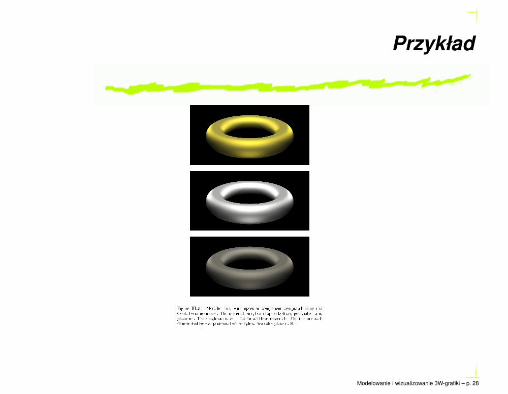
Przykład

Figure III.20: Metalli tori, with spe ular omponent omputed using the

Cook-Torran e model. The materials are, from top to bottom, gold, silver and

platinum. The roughness is m = 0:4 for all three materials. The tori are ea h

illuminated by �ve positional white lights. See olor plate C.16.


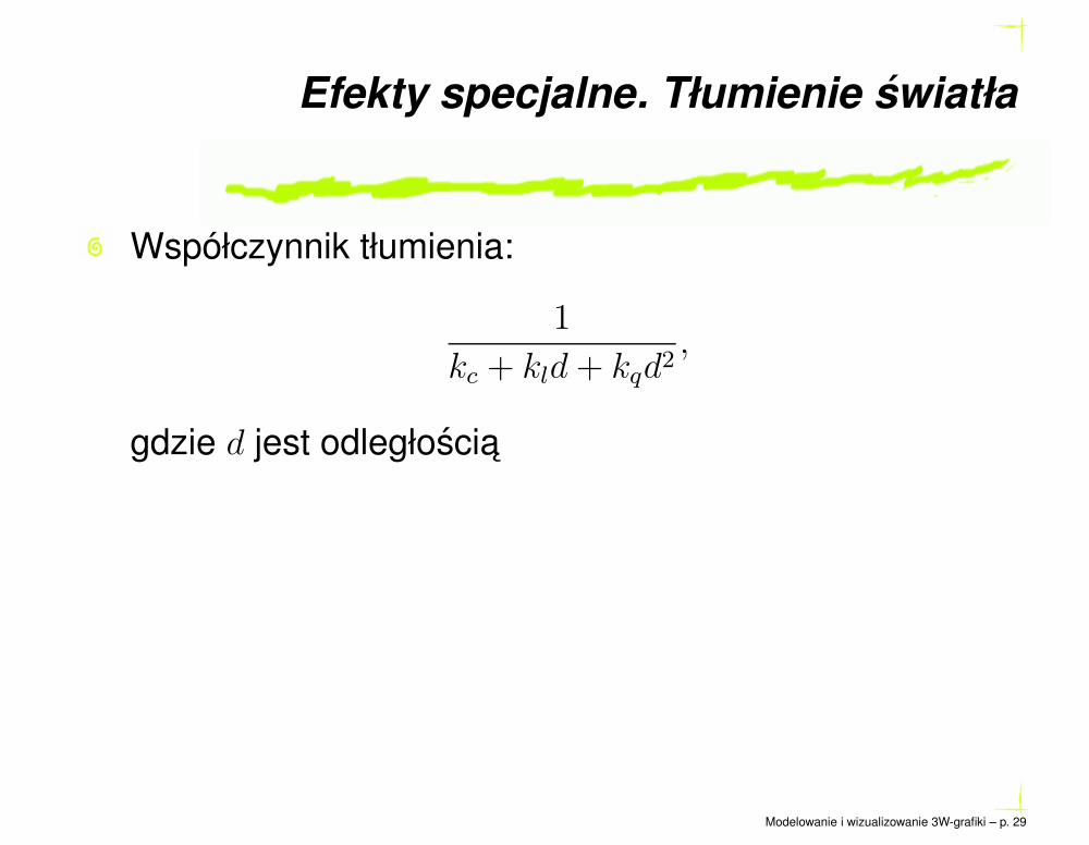
Efekty specjalne. Tłumienie swiatła

Współczynnik tłumienia:

1

kc + kld+ kqd2,

gdzie d jest odległoscia


Efekty specjalne. Swiatło spot

jak swiatło punktowe

kierunek

kat obcinania (cutoff), ψ0

wskaznik tłumienia, p

I =

{

I0(cosψ)p, jezeli ψ < ψ0

0


Efekty specjalne. Swiatło kierunkowe

(Sun)

jak swiatło punktowe

zródło swiata umieszczone jest w nieskonczonosci

(x0 : y0 : z0 : 0)

brak tłumienia (czemu?)


Documents

Oswietlenie i cieniowanie´ - wmii.uwm.edu.plwmii.uwm.edu.pl/~denisjuk/uwm/3d/wyklady/04-oswietlenie.pdf · Modelowanie i wizualizowanie 3W-graﬁki Oswietlenie i cieniowanie´ Aleksander