Nonlinear Earthquake Response Analysis of

Reinforced Concrete Buildings

Lecture Notes

August 2002

Shunsuke Otani Department of Architecture

Graduate School of Engineering University of Tokyo

ii

Preface This note is intended to introduce the state of the art in the nonlinear response analysis of reinforced concrete building structures under earthquake excitation to graduate students. The state of the knowledge on the behavior of reinforced concrete members and structures and the art of nonlinear response analysis are far form an established state. Therefore, this note will not provide any unique solution to a problem. The note was initially prepared for a special lecture on “nonlinear analysis of reinforced concrete buildings” at Department of Civil Engineering, University of Canterbury, New Zealand, from February to April, 1994. The note has been revised for use in Department of Architecture, University of Tokyo since 1996; this course was given in English. The note was extensively revised for a series of lectures on “nonlinear earthquake response analysis of reinforced concrete buildings” at European School for Advanced Studies in Reduction of Seismic Risk, Universita degli Studi di Pavia, Italy, from February to March, 2002. The use of this note should be limited to personal use. August 2002 Professor Shunsuke Otani Department of Architecture, Graduate School of Engineering University of Tokyo otani@sake.t.u-tokyo.ac.jp http://www.rcs.arch.t.u-tokyo.ac.jp/otani/

iii

Contents of Lecture

1. Introduction 2. Properties of Reinforced Concrete Materials 2.1 Concrete 2.2 Reinforcing Steel 2.3 Bond 3. Behavior of Reinforced Concrete Members 3.1 Behavior of Beams 3.2 Behavior of Columns 3.3 Behavior of Interior Beam-column Connections 3.4 Behavior of Exterior Beam-column Connections 3.5 Behavior of Structural Walls 4. Analysis of Reinforced Concrete Members 4.1 Flexural Analysis of Section 4.2 Moment-Curvature Relation under Reversed Loading 4.3 Flexural Analysis of Members 4.4 Load-deformation Relation of Beams 4.5 Analysis of Structural Walls 5. Structural Dynamics 5.1 Differential Equation of Motion 5.2 Mass of Inertia 5.3 Damping 5.4 Strain-rate Effect 5.5 Properties of Earthquake Ground Motion 6. Numerical Integration Methods 6.1 Introduction 6.2 Nigam-Jennings’ Direct Integration Method 6.3 Linear Acceleration Method 6.4 Newmark Beta Method 6.5 Wilson’s Theta Method 6.6 Runge-Kutta-Gill Method (Fourth Order) 7. Matrix Analysis of Linearly Elastic Plane Frames 7.1 Assumptions 7.2 Member Stiffness Matrix in Local Coordinates 7.3 Coordinate Transformation 7.4 Member Stiffness Matrix in Global Coordinates 7.5 Continuity of Displacement at Joint 7.6 Equilibrium of Forces at Joint 7.7 Formulation of Structural Stiffness Matrix 7.8 Free Joint Displacements and Support Reactions 7.9 Member End Actions 8. Numerical Solution of Linear Equations 8.1 Incremental Formulation 8.2 Modified Cholesky Matrix Decomposition 8.3 Solution of Linear Algebraic Equations 8.4 Static Condensation 8.5 Damping Matrix

iv

9. Formulation of Member Stiffness Matrix 9.1 Introduction 9.2 Formulation of Member Stiffness Matrix 9.3 Member with Rigid Ends 9.4 Member with Flexible Ends 9.5 Simply Supported Member 10. Member Stiffness Models 10.1 Member Stiffness Model 10.2 Fiber Model 10.3 Discrete Element Models 10.4 One-component Model 10.5 Multi-component Model 10.6 Distributed Flexibility Model 10.7 Multi-spring Model (1) 10.8 Multi-spring Model (2) 10.9 Multi-spring Model (3) 10.10 Wall Models 11. Member Hysteresis Models 11.1 Introduction 11.2 Bilinear Model 11.3 Ramberg-Osgood Model 11.4 Degrading Trilinear Model 11.5 Clough Degrading Model 11.6 Takeda Degrading Model 11.7 Pivot Model 11.8 Stable Hysteresis Models with Pinching 11.9 Shear-type Hysteresis Models 11.10 Axial Force-Bending Moment Interaction 11.11 Special Purpose Models 12. Response of Different Models 12.1 Effect of Member Modeling 12.2 Effect of Damping Modeling 13. Response of Different Hysteresis Models 13.1 Analysis Method 13.2 Effect of Initial Stiffness (Takeda Model) 13.3 Effect of Cracking Force Level (Takeda Model) 13.4 Effect of Yield Resistance Level (Takeda Model) 13.5 Effect of Post-Yielding Stiffness (Takeda Model) 13.6 Effect of Unloading Stiffness Degradation Parameters (Takeda Model) 13.7 Effect of Hysteresis Energy Dissipation 13.8 Effect of Parameter of Ramberg-Osgood Model 13.9 Response to Different Earthquake Motions 13.10 Response of Different Models 13.11 Response Waveforms and Hysteresis Relations 13.12 Effect of Hysteresis Shape on Frame Response 1４. Reliability of Nonlinear Response Analysis Methods 14.1 Introduction 14.2 Reinforced Concrete Column 14.3 Frame Structures 14.4 Frame-wall Structures 14.5 Wall Structures

v

15. U.S.-Japan Full-scale Test 15.1 Test Program of Full-scale Seven-story RC Building 15.2 Description of Test 15.3 Modeling of Structural Members 15.4 Stiffness of Member Models 15.5 Method of Response Analysis 15.6 Results of Analysis 15.7 Concluding Remarks

Suggested Reading American Concrete Institute, Earthquake Resistant Concrete Structures - Inelastic Response and

Design, ACI-SP127, American Concrete Institute, Detroit, 1991. Comite Euro-International du Beton, RC Elements under Cyclic Loading - State of the Art Report,

Thomas Telford, 1996, 190 pp. Comite Euro-International du Beton, RC Frames under Earthquake Loading - State of the Art Report,

Thomas Telford, 1996, 303 pp.

1

Chapter 1. INTRODUCTION

Dynamic response of a structure can be caused by different loading conditions such as: (a) earthquake ground motion; (b) wind pressure; (c) wave action; (d) blast; (e) machine vibration; and (f) traffic movement. Among these, inelastic response is mainly caused by earthquake motions and accidental blasts. Consequently, more research on nonlinear structural behaviour has been carried out in relation to earthquake problems.

1.1 Structural Dynamics Note that dynamic problems are different from static one in the following points: (a) inertial force;

(b) damping; (c) strain rate effect; and (d) oscillation (stress reversals). These need to be clarified in order to analyze a structure under dynamic loading.

The equation of motion for a linearly elastic system under horizontal ground motion is normally

expressed in a form below; [ ]{ } [ ]{ } [ ]{ } {0}m z c x k x+ + =

where [ ]m , [ ]c , [ ]k : mass, damping coefficient and stiffness matrices, { }z : absolute acceleration vector at mass level, { }x and { }x : velocity and displacement vector at mass level relative to the structural foundation.

Dynamic characteristics up to failure cannot be identified solely through a dynamic test of a real

structure for the following reasons: (a) difficult to understand the behaviour due to complex interactions of various parameters; (b) expensive to build a structure, as a specimen, for destructive testing; and (c) capacity of loading devices insufficient to cause failure. Consequently, dynamic tests of real buildings are rather aimed toward obtaining data (a) to confirm the validity of mathematical modeling techniques for a linearly elastic structure; and (b) to obtain damping characteristics of different types of structures. A specifically designed laboratory test becomes inevitable in order to complement the weakness of full-scale tests and to study the effect of individual parameters. Damping: Any mechanical system possesses some energy-dissipating mechanisms, for example: (a) inelastic hysteretic energy dissipation; (b) radiation of kinetic energy through foundation; (c) kinetic friction; (d) viscosity in materials; and (e) aerodynamic effect. Such capacity or energy dissipation is vaguely termed “damping,” and is most often assumed to be of viscous type simply because of its mathematical simplicity; i.e., resistance proportional to velocity. It should be noted that the actual damping mechanism may not be of viscous type.

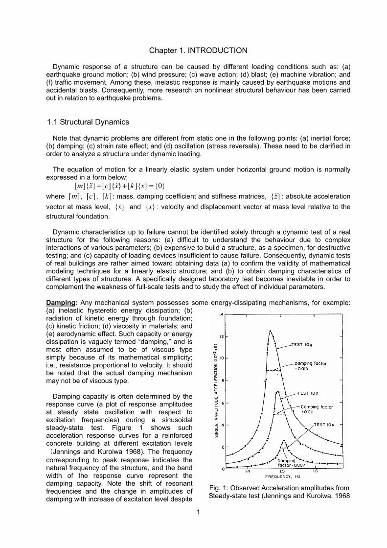
Damping capacity is often determined by the

response curve (a plot of response amplitudes at steady state oscillation with respect to excitation frequencies) during a sinusoidal steady-state test. Figure 1 shows such acceleration response curves for a reinforced concrete building at different excitation levels（Jennings and Kuroiwa 1968). The frequency corresponding to peak response indicates the natural frequency of the structure, and the band width of the response curve represent the damping capacity. Note the shift of resonant frequencies and the change in amplitudes of damping with increase of excitation level despite

Fig. 1: Observed Acceleration amplitudes from Steady-state test (Jennings and Kuroiwa, 1968

2

low response amplitudes. Damping capacity, expressed in terms of viscous damping factor, is not a unique value of a

structure, but it depends on the level of excitation. The state-of-the-art does not provide a method to determine the damping capacity based on the material properties and geometrical characteristics of a structure.

Strain Rate Effect: It is technically difficult to test structural members under dynamic conditions in a laboratory. Before force-deformation relations already obtained from thousands of static tests can be studied for use in a dynamic analysis, the effect of strain rate on the force-deformation relation needs to be examined.

The speed of loading is known to influence the stiffness and strength of various materials (Cowell

1965, 1966). Some member test results are available (Mahin and Bertero l972). Important findings from these investigations are as follows: (a) high strain rates increased the initial yield resistance, but caused small differences in either stiffness or resistance in subsequent cycles at the same displacement amplitudes; (b) strain rate effect on resistance diminished with increased deformation in a strain-hardening range; and (c) no substantial changes were observed in ductility and overall energy absorption capacity.

Note that strain rate (velocity) during an oscillation is highest at low stress levels, and that the rate

gradually decreases toward a peak strain. Cracking and yielding of a reinforced concrete member reduce the stiffness, elongating the period of oscillation. Furthermore, such damage is normally caused by the lower modes of vibration having long periods. Therefore, the strain rate is small in the case of earthquake response, and its effect on the response is small.

Consequently, the static hysteretic behaviour observed can be utilized in a nonlinear dynamic

analysis of reinforced concrete structures.

1.2 Stiffness Properties of Reinforced Concrete Members It is not feasible to analyze an entire structure using microscopic material models. It is more

important to study the behaviour of isolated members and their subassemblies (beam-column, slab-column, and slab-wall connections) so that their analytical models can be developed for use in the analysis of a complete structure.

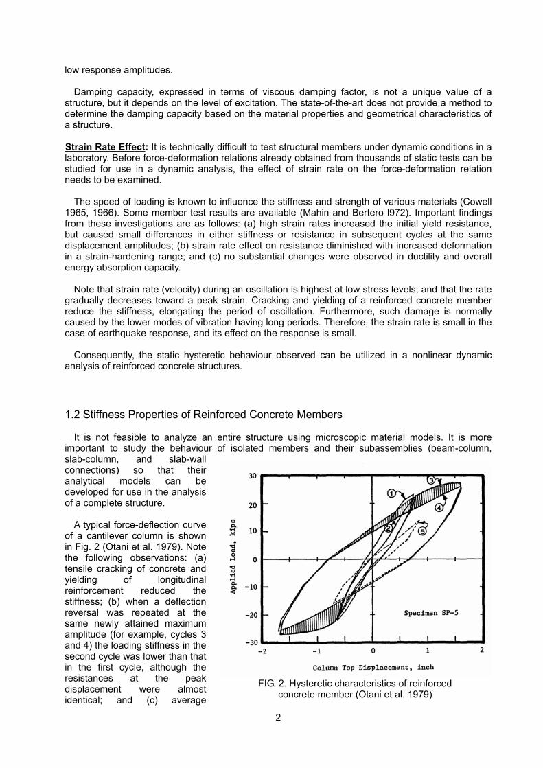
A typical force-deflection curve

of a cantilever column is shown in Fig. 2 (Otani et al. 1979). Note the following observations: (a) tensile cracking of concrete and yielding of longitudinal reinforcement reduced the stiffness; (b) when a deflection reversal was repeated at the same newly attained maximum amplitude (for example, cycles 3 and 4) the loading stiffness in the second cycle was lower than that in the first cycle, although the resistances at the peak displacement were almost identical; and (c) average

FIG. 2. Hysteretic characteristics of reinforced concrete member (Otani et al. 1979)

3

stiffness (peak-to-peak) of a complete cycle decreased with a maximum displacement amplitude. For example, the peak-to-peak stiffness of cycle 5, after large amplitude displacement reversals, was significantly reduced from that of cycle 2 at comparable displacement amplitudes. Therefore, the hysteretic behaviour of the reinforced concrete is sensitive to loading history. Let us study some typical stiffness characteristics of reinforced concrete.

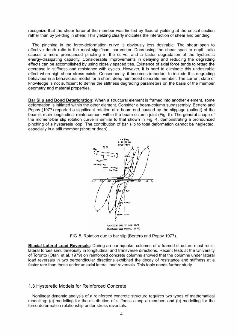
Flexural Characteristics: The flexural deformation index (average curvature) is obtained from longitudinal strain measurements at two levels assuming that a plane section remains plane. This flexural deformation index does not represent the flexural deformation in a strict sense because a plane section does not remain plane in a region where an extensive shear deformation occurs. However, the index is useful for understanding flexural deformation characteristics qualitatively.

A typical moment-flexural

deformation index curve obtained from a simply supported beam test (Celebi and Penzien 1973) is shown.in Fig. 3. Note that the stiffness during loading gradually decreases with load, forming a fat hysteresis loop, and absorbing a large amount of hysteretic energy. The hysteresis loops remain almost identical even after several load reversals at the same displacement amplitude beyond yielding. Consequently, vibration energy can be efficiently dissipated through flexural hysteresis loops without a reduction in resistance. Many hysteretic models, as discussed later, are currently available to represent the nexural behaviour.

The increase in axial force decreases the flexural ductility of a reinforced concrete member, but

increases force levels corresponding to (a) tensile cracking of concrete; and (b) tensile yielding of longitudinal reinforcement.

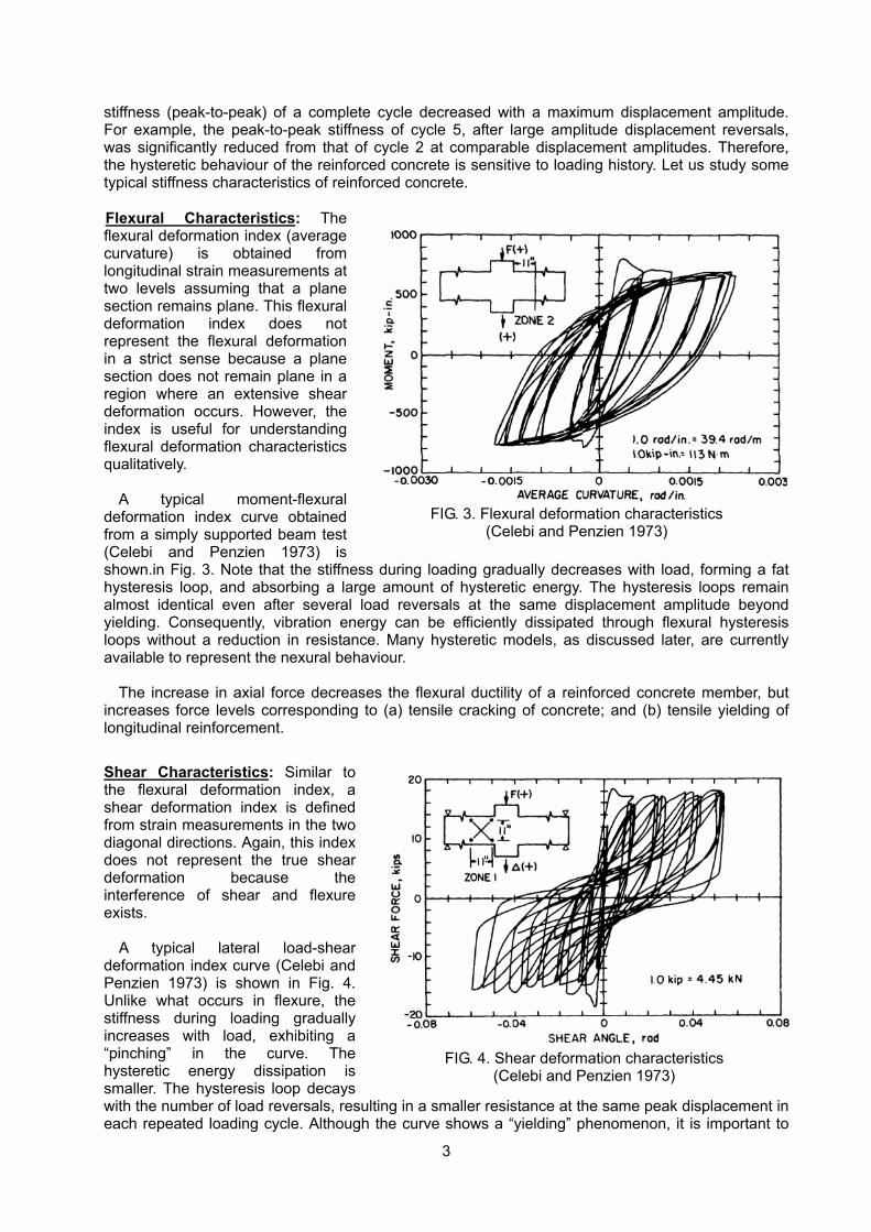
Shear Characteristics: Similar to the flexural deformation index, a shear deformation index is defined from strain measurements in the two diagonal directions. Again, this index does not represent the true shear deformation because the interference of shear and flexure exists.

A typical lateral load-shear

deformation index curve (Celebi and Penzien 1973) is shown in Fig. 4. Unlike what occurs in flexure, the stiffness during loading gradually increases with load, exhibiting a “pinching” in the curve. The hysteretic energy dissipation is smaller. The hysteresis loop decays with the number of load reversals, resulting in a smaller resistance at the same peak displacement in each repeated loading cycle. Although the curve shows a “yielding” phenomenon, it is important to

FIG. 4. Shear deformation characteristics (Celebi and Penzien 1973)

FIG. 3. Flexural deformation characteristics (Celebi and Penzien 1973)

4

recognize that the shear force of the member was limited by flexural yielding at the critical section rather than by yielding in shear. This yielding clearly indicates the interaction of shear and bending.

The pinching in the force-deformation curve is obviously less desirable. The shear span to

effective depth ratio is the most significant parameter. Decreasing the shear span to depth ratio causes a more pronounced pinching in the curve, and a faster degradation of the hysteretic energy-dissipating capacity. Considerable improvements in delaying and reducing the degrading effects can be accomplished by using closely spaced ties. Existence of axial force tends to retard the decrease in stiffness and resistance with cycles. However, it is hard to eliminate this undesirable effect when high shear stress exists. Consequently, it becomes important to include this degrading behaviour in a behavioural model for a short, deep reinforced concrete member. The current state of knowledge is not sufficient to define the stiffness degrading parameters on the basis of the member geometry and material properties.

Bar Slip and Bond Deterioration: When a structural element is framed into another element, some deformation is initiated within the other element. Consider a beam-column subassembly. Bertero and Popov (1977) reported a significant rotation at a beam end caused by the slippage (pullout) of the beam's main longitudinal reinforcement within the beam-column joint (Fig. 5). The general shape of the moment-bar slip rotation curve is similar to that shown in Fig. 4, demonstrating a pronounced pinching of a hysteresis loop. The contribution of bar slip to total deformation cannot be neglected, especially in a stiff member (short or deep).

FIG. 5. Rotation due to bar slip (Bertero and Popov 1977).

Biaxial Lateral Load Reversals: During an earthquake, columns of a framed structure must resist lateral forces simultaneously in longitudinal and transverse directions. Recent tests at the University of Toronto (Otani et al. 1979) on reinforced concrete columns showed that the columns under lateral load reversals in two perpendicular directions exhibited the decay of resistance and stiffness at a faster rate than those under uniaxial lateral load reversals. This topic needs further study.

1.3 Hysteretic Models for Reinforced Concrete Nonlinear dynamic analysis of a reinforced concrete structure requires two types of mathematical

modelling: (a) modelling for the distribution of stiffness along a member; and (b) modelling for the force-deformation relationship under stress reversals.

5

A hysteresis model must be able to provide the stiffness and resistance under any displacement

history. At the same time, the basic characteristics need to be defined by the member geometry and material properties. The current state of knowledge is sufficient to define flexural hysteresis models. However, it is not sufficient to determine the degree of stiffness degradation due to the deterioration of shear-resisting and rebar-concrete bond mechanisms.

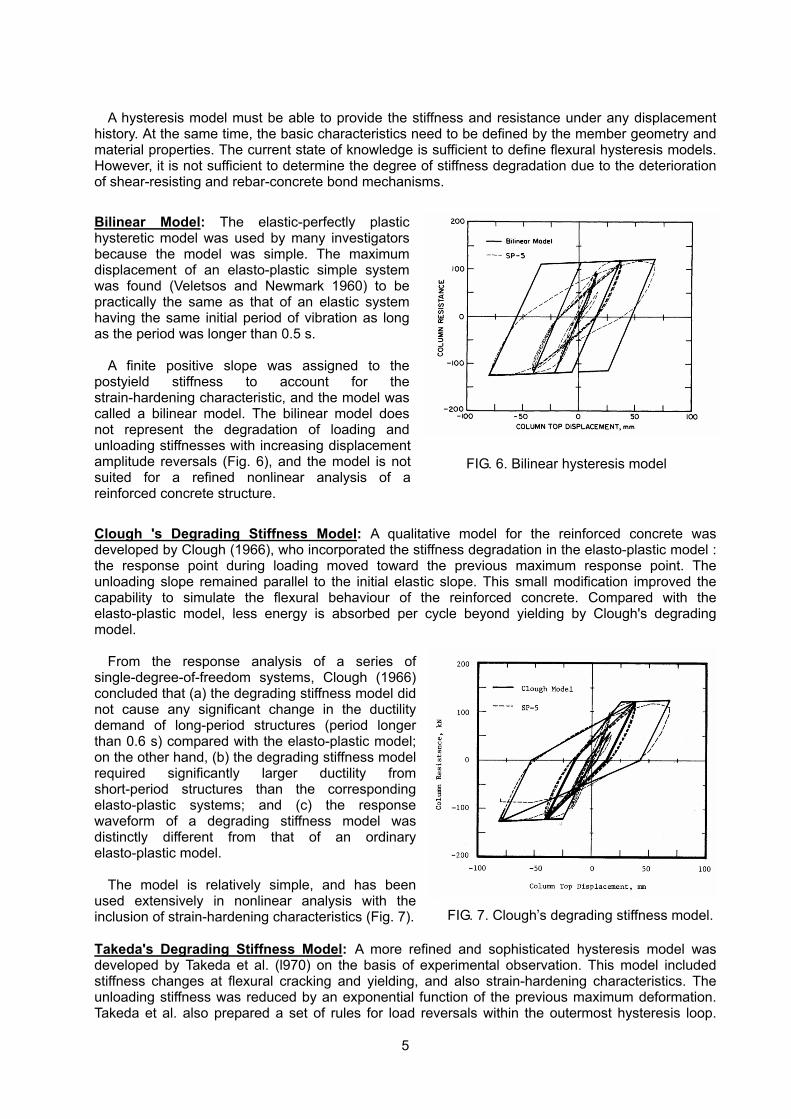
Bilinear Model: The elastic-perfectly plastic hysteretic model was used by many investigators because the model was simple. The maximum displacement of an elasto-plastic simple system was found (Veletsos and Newmark 1960) to be practically the same as that of an elastic system having the same initial period of vibration as long as the period was longer than 0.5 s.

A finite positive slope was assigned to the

postyield stiffness to account for the strain-hardening characteristic, and the model was called a bilinear model. The bilinear model does not represent the degradation of loading and unloading stiffnesses with increasing displacement amplitude reversals (Fig. 6), and the model is not suited for a refined nonlinear analysis of a reinforced concrete structure.

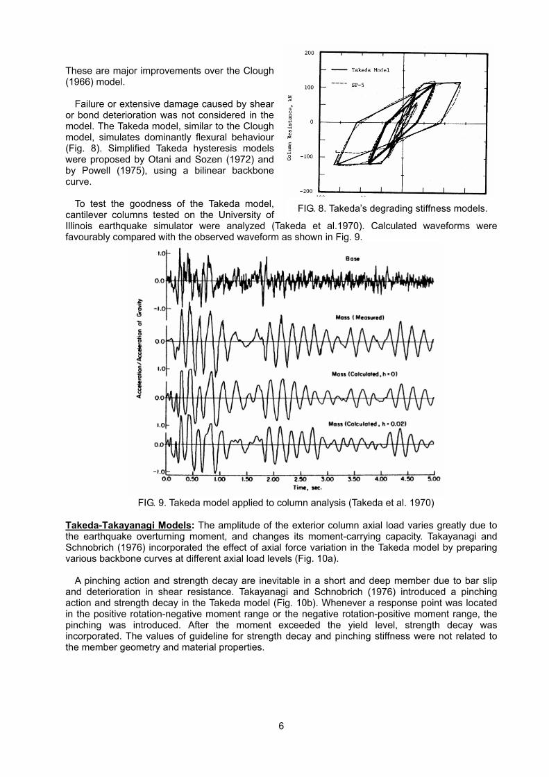
Clough 's Degrading Stiffness Model: A qualitative model for the reinforced concrete was developed by Clough (1966), who incorporated the stiffness degradation in the elasto-plastic model : the response point during loading moved toward the previous maximum response point. The unloading slope remained parallel to the initial elastic slope. This small modification improved the capability to simulate the flexural behaviour of the reinforced concrete. Compared with the elasto-plastic model, less energy is absorbed per cycle beyond yielding by Clough's degrading model.

From the response analysis of a series of

single-degree-of-freedom systems, Clough (1966) concluded that (a) the degrading stiffness model did not cause any significant change in the ductility demand of long-period structures (period longer than 0.6 s) compared with the elasto-plastic model; on the other hand, (b) the degrading stiffness model required significantly larger ductility from short-period structures than the corresponding elasto-plastic systems; and (c) the response waveform of a degrading stiffness model was distinctly different from that of an ordinary elasto-plastic model.

The model is relatively simple, and has been

used extensively in nonlinear analysis with the inclusion of strain-hardening characteristics (Fig. 7).

Takeda's Degrading Stiffness Model: A more refined and sophisticated hysteresis model was developed by Takeda et al. (l970) on the basis of experimental observation. This model included stiffness changes at flexural cracking and yielding, and also strain-hardening characteristics. The unloading stiffness was reduced by an exponential function of the previous maximum deformation. Takeda et al. also prepared a set of rules for load reversals within the outermost hysteresis loop.

FIG. 6. Bilinear hysteresis model

FIG. 7. Clough’s degrading stiffness model.

6

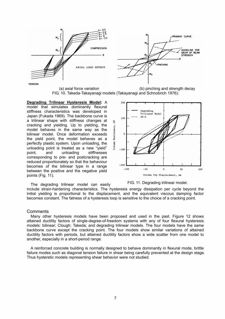
These are major improvements over the Clough (1966) model.

Failure or extensive damage caused by shear

or bond deterioration was not considered in the model. The Takeda model, similar to the Clough model, simulates dominantly flexural behaviour (Fig. 8). Simplified Takeda hysteresis models were proposed by Otani and Sozen (1972) and by Powell (1975), using a bilinear backbone curve.

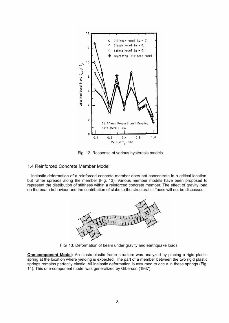
To test the goodness of the Takeda model,

cantilever columns tested on the University of Illinois earthquake simulator were analyzed (Takeda et al.1970). Calculated waveforms were favourably compared with the observed waveform as shown in Fig. 9.

FIG. 9. Takeda model applied to column analysis (Takeda et al. 1970)

Takeda-Takayanagi Models: The amplitude of the exterior column axial load varies greatly due to the earthquake overturning moment, and changes its moment-carrying capacity. Takayanagi and Schnobrich (1976) incorporated the effect of axial force variation in the Takeda model by preparing various backbone curves at different axial load levels (Fig. 10a).

A pinching action and strength decay are inevitable in a short and deep member due to bar slip and deterioration in shear resistance. Takayanagi and Schnobrich (1976) introduced a pinching action and strength decay in the Takeda model (Fig. 10b). Whenever a response point was located in the positive rotation-negative moment range or the negative rotation-positive moment range, the pinching was introduced. After the moment exceeded the yield level, strength decay was incorporated. The values of guideline for strength decay and pinching stiffness were not related to the member geometry and material properties.

FIG. 8. Takeda’s degrading stiffness models.

7

(a) axial force variation (b) pinching and strength decay

FIG. 10. Takeda-Takayanagi models (Takayanagi and Schnobrich 1976): Degrading Trilinear Hysteresis Model: A model that simulates dominantly flexural stiffness characteristics was developed in Japan (Fukada 1969). The backbone curve is a trilinear shape with stiffness changes at cracking and yielding. Up to yielding, the model behaves in the same way as the bilinear model. Once deformation exceeds the yield point, the model behaves as a perfectly plastic system. Upon unloading, the unloading point is treated as a new “yield” point, and unloading stiffnesses corresponding to pre- and postcracking are reduced proportionately so that the behaviour becomes of the bilinear type in a range between the positive and the negative yield points (Fig. 11).

The degrading trilinear model can easily

include strain-hardening characteristics. The hysteresis energy dissipation per cycle beyond the initial yielding is proportional to the displacement, and the equivalent viscous damping factor becomes constant. The fatness of a hysteresis loop is sensitive to the choice of a cracking point.

Comments Many other hysteresis models have been proposed and used in the past. Figure 12 shows

attained ductility factors of single-degree-of-freedom systems with any of four flexural hysteresis models: bilinear; Clough; Takeda; and degrading trilinear models. The four models have the same backbone curve except the cracking point. The four models show similar variations of attained ductility factors with periods, but attained ductility factors show a wide scatter from one model to another, especially in a short-period range.

A reinforced concrete building is normally designed to behave dominantly in flexural mode, brittle

failure modes such as diagonal tension failure in shear being carefully prevented at the design stage. Thus hysteretic models representing shear behavior were not studied.

FIG. 11. Degrading trilinear model.

8

1.4 Reinforced Concrete Member Model

Inelastic deformation of a reinforced concrete member does not concentrate in a critical location, but rather spreads along the member (Fig. 13). Various member models have been proposed to represent the distribution of stiffness within a reinforced concrete member. The effect of gravity load on the beam behaviour and the contribution of slabs to the structural stiffness will not be discussed.

FIG. 13. Deformation of beam under gravity and earthquake loads.

One-component Model: An elasto-plastic frame structure was analyzed by placing a rigid plastic spring at the location where yielding is expected. The part of a member between the two rigid plastic springs remains perfectly elastic. All inelastic deformation is assumed to occur in these springs (Fig. 14). This one-component model was generalized by Giberson (1967).

Fig. 12. Response of various hysteresis models

9

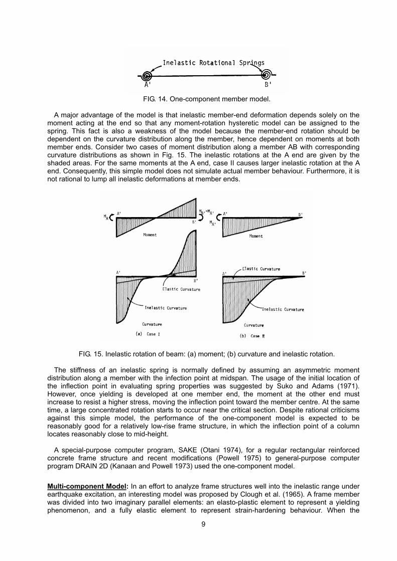
FIG. 14. One-component member model.

A major advantage of the model is that inelastic member-end deformation depends solely on the

moment acting at the end so that any moment-rotation hysteretic model can be assigned to the spring. This fact is also a weakness of the model because the member-end rotation should be dependent on the curvature distribution along the member, hence dependent on moments at both member ends. Consider two cases of moment distribution along a member AB with corresponding curvature distributions as shown in Fig. 15. The inelastic rotations at the A end are given by the shaded areas. For the same moments at the A end, case II causes larger inelastic rotation at the A end. Consequently, this simple model does not simulate actual member behaviour. Furthermore, it is not rational to lump all inelastic deformations at member ends.

FIG. 15. Inelastic rotation of beam: (a) moment; (b) curvature and inelastic rotation. The stiffness of an inelastic spring is normally defined by assuming an asymmetric moment

distribution along a member with the infection point at midspan. The usage of the initial location of the inflection point in evaluating spring properties was suggested by Suko and Adams (1971). However, once yielding is developed at one member end, the moment at the other end must increase to resist a higher stress, moving the inflection point toward the member centre. At the same time, a large concentrated rotation starts to occur near the critical section. Despite rational criticisms against this simple model, the performance of the one-component model is expected to be reasonably good for a relatively low-rise frame structure, in which the inflection point of a column locates reasonably close to mid-height.

A special-purpose computer program, SAKE (Otani 1974), for a regular rectangular reinforced

concrete frame structure and recent modifications (Powell 1975) to general-purpose computer program DRAIN 2D (Kanaan and Powell 1973) used the one-component model.

Multi-component Model: In an effort to analyze frame structures well into the inelastic range under earthquake excitation, an interesting model was proposed by Clough et al. (1965). A frame member was divided into two imaginary parallel elements: an elasto-plastic element to represent a yielding phenomenon, and a fully elastic element to represent strain-hardening behaviour. When the

10

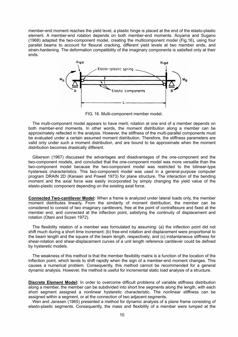
member-end moment reaches the yield level, a plastic hinge is placed at the end of the elasto-plastic element. A member-end rotation depends on both member-end moments. Aoyama and Sugano (1968) adapted the two-component model, creating the multicomponent model (Fig.16), using four parallel beams to account for flexural cracking, different yield levels at two member ends, and strain-hardening. The deformation compatibility of the imaginary components is satisfied only at their ends.

FIG. 16. Multi-component member model.

The multi-component model appears to have merit; rotation at one end of a member depends on

both member-end moments. In other words, the moment distribution along a member can be approximately reflected in the analysis. However, the stiffness of the multi-parallel components must be evaluated under a certain assumed moment distribution. Therefore, the stiffness parameters are valid only under such a moment distribution, and are bound to be approximate when the moment distribution becomes drastically different.

Giberson (1967) discussed the advantages and disadvantages of the one-component and the

two-component models, and concluded that the one-component model was more versatile than the two-component model because the two-component model was restricted to the bilinear-type hysteresis characteristics. This two-component model was used in a general-purpose computer program DRAIN 2D (Kanaan and Powell 1973) for plane structure. The interaction of the bending moment and the axial force was easily incorporated by simply changing the yield value of the elasto-plastic component depending on the existing axial force.

Connected Two-cantilever Model: When a frame is analyzed under lateral loads only, the member moment distributes linearly. From the similarity of moment distribution, the member can be considered to consist of two imaginary cantilevers, free at the point of contraflexure and fixed at the member end, and connected at the inflection point, satisfying the continuity of displacement and rotation (Otani and Sozen 1972).

The flexibility relation of a member was formulated by assuming: (a) the inflection point did not

shift much during a short time increment; (b) free-end rotation and displacement were proportional to the beam length and the square of the beam length, respectively; and (c) instantaneous stiffness for shear-rotation and shear-displacement curves of a unit length reference cantilever could be defined by hysteretic models.

The weakness of this method is that the member flexibility matrix is a function of the location of the

inflection point, which tends to shift rapidly when the sign of a member-end moment changes. This causes a numerical problem. Consequently, this method cannot be recommended for a general dynamic analysis. However, the method is useful for incremental static load analysis of a structure.

Discrete Element Model: In order to overcome difficult problems of variable stiffness distribution along a member, the member can be subdivided into short line segments along the length, with each short segment assigned a nonlinear hysteretic characteristic. The nonlinear stiffness can be assigned within a segment, or at the connection of two adjacent segments.

Wen and Janssen (1965) presented a method for dynamic analysis of a plane frame consisting of elasto-plastic segments. Consequently, the mass and flexibility of a member were lumped at the

11

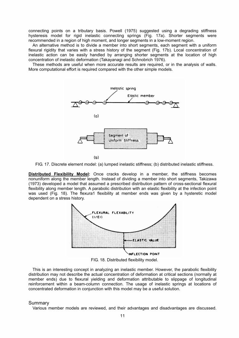
connecting points on a tributary basis. Powell (1975) suggested using a degrading stiffness hysteresis model for rigid inelastic connecting springs (Fig. 17a). Shorter segments were recommended in a region of high moment, and longer segments in a low-moment region.

An alternative method is to divide a member into short segments, each segment with a uniform flexural rigidity that varies with a stress history of the segment (Fig. 17b). Local concentration of inelastic action can be easily handled by arranging shorter segments at the location of high concentration of inelastic deformation (Takayanagi and Schnobrich 1976).

These methods are useful when more accurate results are required, or in the analysis of walls. More computational effort is required compared with the other simple models.

FIG. 17. Discrete element model: (a) lumped inelastic stiffness; (b) distributed inelastic stiffness.

Distributed Flexibility Model: Once cracks develop in a member, the stiffness becomes nonuniform along the member length. Instead of dividing a member into short segments, Takizawa (1973) developed a model that assumed a prescribed distribution pattern of cross-sectional flexural flexibility along member length. A parabolic distribution with an elastic flexibility at the infection point was used (Fig. 18). The flexura1 flexibility at member ends was given by a hysteretic model dependent on a stress history.

FIG. 18. Distributed flexibility model.

This is an interesting concept in analyzing an inelastic member. However, the parabolic flexibility

distribution may not describe the actual concentration of deformation at critical sections (normally at member ends) due to flexural yielding and deformation attributable to slippage of longitudinal reinforcement within a beam-column connection. The usage of inelastic springs at locations of concentrated deformation in conjunction with this model may be a useful solution.

Summary Various member models are reviewed, and their advantages and disadvantages are discussed.

12

These models have been developed specifically for earthquake response. Development of a simple model for simultaneous gravity and earthquake situations is desired.

Member stiffness matrix, equilibrium of forces and continuity of displacement at joints are used to formulate a series of linear equations under a given loading condition. Numerical integration methods are used to solve the equation of motion under dynamic loading conditions. The response of a structural model is evaluated by solving the set of linear equation incremental time steps.

1.5 Reliability of Analytical Models

Earthquake simulator tests provide interesting opportunities to examine the goodness of different analytical models in simulating the observed response of small- to medium-scale highly inelastic model structures. This section reviews the reliability of different analytical models in relation to the capability to simulate the observed behaviour.

These test structures were designed to behave dominantly in flexure, being prevented as much

as possible from failing in shear or anchorage because the two types of failure are not desirable in real construction and are avoided in a design process.

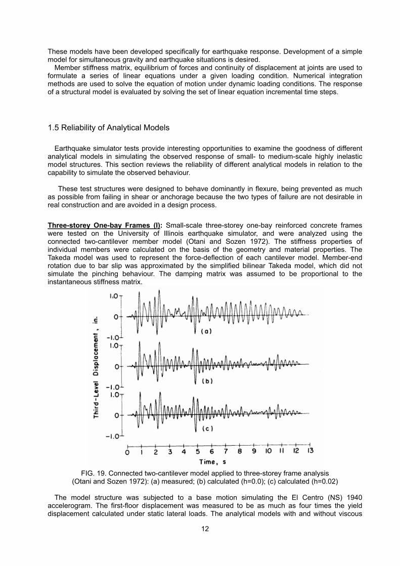
Three-storey One-bay Frames (I): Small-scale three-storey one-bay reinforced concrete frames were tested on the University of Illinois earthquake simulator, and were analyzed using the connected two-cantilever member model (Otani and Sozen 1972). The stiffness properties of individual members were calculated on the basis of the geometry and material properties. The Takeda model was used to represent the force-deflection of each cantilever model. Member-end rotation due to bar slip was approximated by the simplified bilinear Takeda model, which did not simulate the pinching behaviour. The damping matrix was assumed to be proportional to the instantaneous stiffness matrix.

FIG. 19. Connected two-cantilever model applied to three-storey frame analysis

(Otani and Sozen 1972): (a) measured; (b) calculated (h=0.0); (c) calculated (h=0.02) The model structure was subjected to a base motion simulating the El Centro (NS) 1940

accelerogram. The first-floor displacement was measured to be as much as four times the yield displacement calculated under static lateral loads. The analytical models with and without viscous

13

damping favourably simulated the large-amplitude oscillations at 1.0, 2.0, and 5 s from the beginning of the motion (Fig. 19). The analytical models, however, failed to simulate the medium- and low-amplitude oscillations. Note that the frequencies at the medium- to low-amplitude oscillations are higher for the analytical model, which indicates that the test structure was more flexible at low stress levels than the analytical model. In order to reproduce lower amplitude oscillations of the observed response waveforms, the pinching behaviour needs to be incorporated in a hysteretic model.

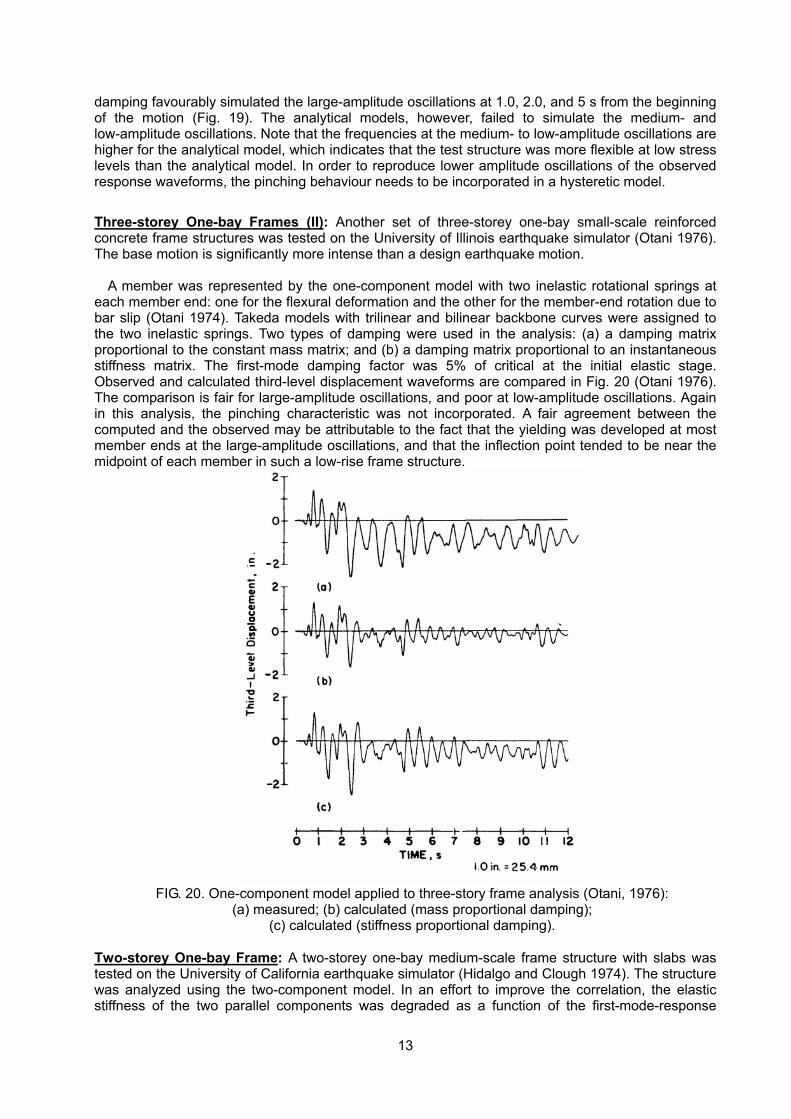
Three-storey One-bay Frames (II): Another set of three-storey one-bay small-scale reinforced concrete frame structures was tested on the University of Illinois earthquake simulator (Otani 1976). The base motion is significantly more intense than a design earthquake motion.

A member was represented by the one-component model with two inelastic rotational springs at

each member end: one for the flexural deformation and the other for the member-end rotation due to bar slip (Otani 1974). Takeda models with trilinear and bilinear backbone curves were assigned to the two inelastic springs. Two types of damping were used in the analysis: (a) a damping matrix proportional to the constant mass matrix; and (b) a damping matrix proportional to an instantaneous stiffness matrix. The first-mode damping factor was 5% of critical at the initial elastic stage. Observed and calculated third-level displacement waveforms are compared in Fig. 20 (Otani 1976). The comparison is fair for large-amplitude oscillations, and poor at low-amplitude oscillations. Again in this analysis, the pinching characteristic was not incorporated. A fair agreement between the computed and the observed may be attributable to the fact that the yielding was developed at most member ends at the large-amplitude oscillations, and that the inflection point tended to be near the midpoint of each member in such a low-rise frame structure.

FIG. 20. One-component model applied to three-story frame analysis (Otani, 1976):

(a) measured; (b) calculated (mass proportional damping); (c) calculated (stiffness proportional damping).

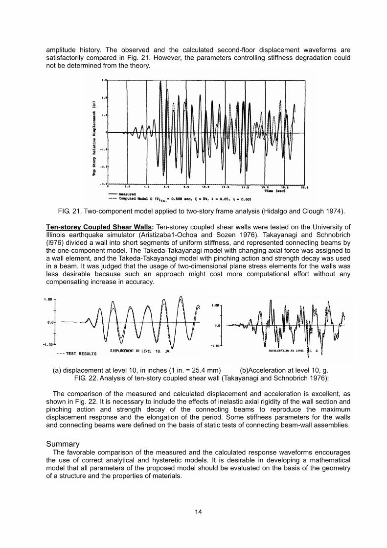
Two-storey One-bay Frame: A two-storey one-bay medium-scale frame structure with slabs was tested on the University of California earthquake simulator (Hidalgo and Clough 1974). The structure was analyzed using the two-component model. In an effort to improve the correlation, the elastic stiffness of the two parallel components was degraded as a function of the first-mode-response

14

amplitude history. The observed and the calculated second-floor displacement waveforms are satisfactorily compared in Fig. 21. However, the parameters controlling stiffness degradation could not be determined from the theory.

FIG. 21. Two-component model applied to two-story frame analysis (Hidalgo and Clough 1974).

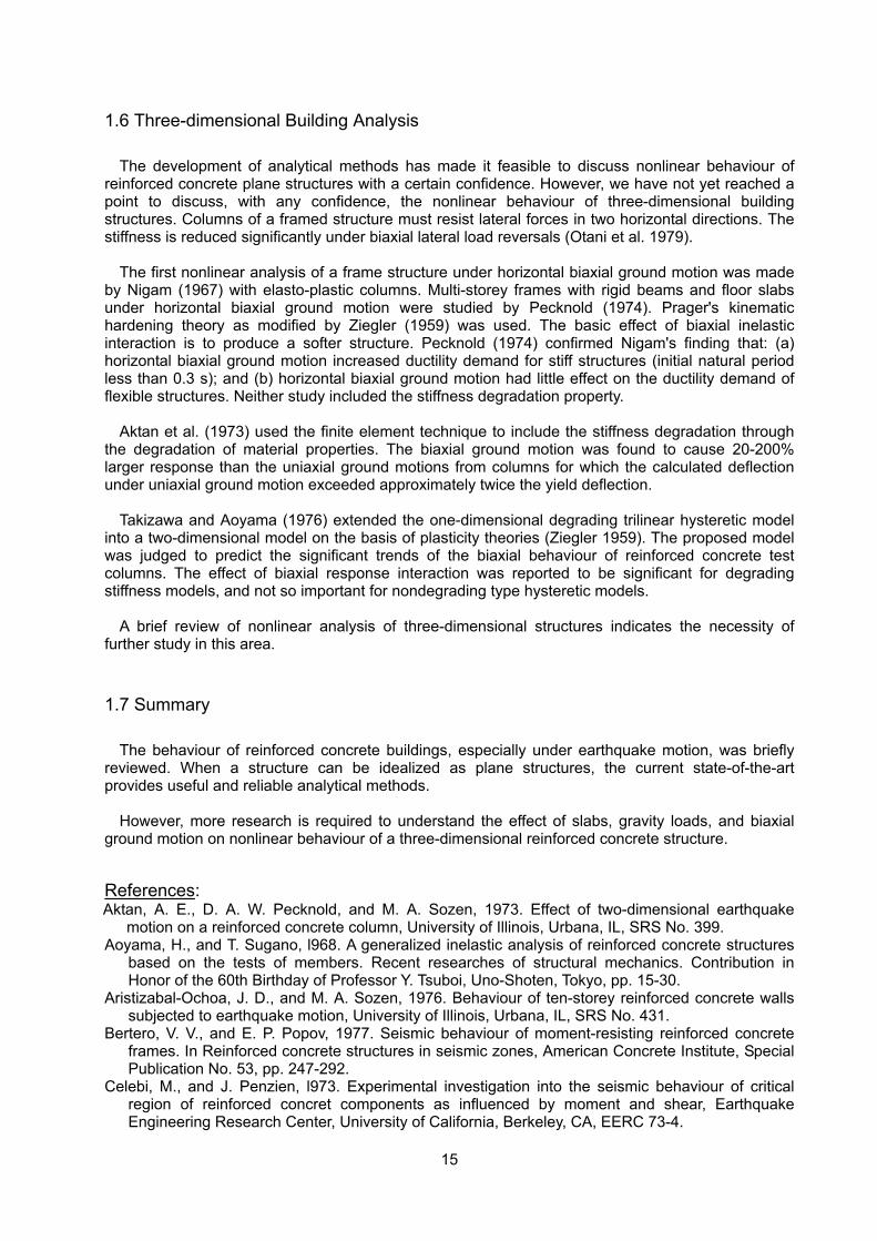
Ten-storey Coupled Shear Walls: Ten-storey coupled shear walls were tested on the University of Illinois earthquake simulator (Aristizaba1-Ochoa and Sozen 1976). Takayanagi and Schnobrich (l976) divided a wall into short segments of uniform stiffness, and represented connecting beams by the one-component model. The Takeda-Takayanagi model with changing axial force was assigned to a wall element, and the Takeda-Takayanagi model with pinching action and strength decay was used in a beam. It was judged that the usage of two-dimensional plane stress elements for the walls was less desirable because such an approach might cost more computational effort without any compensating increase in accuracy.

(a) displacement at level 10, in inches (1 in. = 25.4 mm) (b)Acceleration at level 10, g.

FIG. 22. Analysis of ten-story coupled shear wall (Takayanagi and Schnobrich 1976): The comparison of the measured and calculated displacement and acceleration is excellent, as

shown in Fig. 22. It is necessary to include the effects of inelastic axial rigidity of the wall section and pinching action and strength decay of the connecting beams to reproduce the maximum displacement response and the elongation of the period. Some stiffness parameters for the walls and connecting beams were defined on the basis of static tests of connecting beam-wall assemblies.

Summary The favorable comparison of the measured and the calculated response waveforms encourages

the use of correct analytical and hysteretic models. It is desirable in developing a mathematical model that all parameters of the proposed model should be evaluated on the basis of the geometry of a structure and the properties of materials.

15

1.6 Three-dimensional Building Analysis

The development of analytical methods has made it feasible to discuss nonlinear behaviour of reinforced concrete plane structures with a certain confidence. However, we have not yet reached a point to discuss, with any confidence, the nonlinear behaviour of three-dimensional building structures. Columns of a framed structure must resist lateral forces in two horizontal directions. The stiffness is reduced significantly under biaxial lateral load reversals (Otani et al. 1979).

The first nonlinear analysis of a frame structure under horizontal biaxial ground motion was made

by Nigam (1967) with elasto-plastic columns. Multi-storey frames with rigid beams and floor slabs under horizontal biaxial ground motion were studied by Pecknold (1974). Prager's kinematic hardening theory as modified by Ziegler (1959) was used. The basic effect of biaxial inelastic interaction is to produce a softer structure. Pecknold (1974) confirmed Nigam's finding that: (a) horizontal biaxial ground motion increased ductility demand for stiff structures (initial natural period less than 0.3 s); and (b) horizontal biaxial ground motion had little effect on the ductility demand of flexible structures. Neither study included the stiffness degradation property.

Aktan et al. (1973) used the finite element technique to include the stiffness degradation through

the degradation of material properties. The biaxial ground motion was found to cause 20-200% larger response than the uniaxial ground motions from columns for which the calculated deflection under uniaxial ground motion exceeded approximately twice the yield deflection.

Takizawa and Aoyama (1976) extended the one-dimensional degrading trilinear hysteretic model

into a two-dimensional model on the basis of plasticity theories (Ziegler 1959). The proposed model was judged to predict the significant trends of the biaxial behaviour of reinforced concrete test columns. The effect of biaxial response interaction was reported to be significant for degrading stiffness models, and not so important for nondegrading type hysteretic models.

A brief review of nonlinear analysis of three-dimensional structures indicates the necessity of

further study in this area.

1.7 Summary

The behaviour of reinforced concrete buildings, especially under earthquake motion, was briefly reviewed. When a structure can be idealized as plane structures, the current state-of-the-art provides useful and reliable analytical methods.

However, more research is required to understand the effect of slabs, gravity loads, and biaxial

ground motion on nonlinear behaviour of a three-dimensional reinforced concrete structure.

References: Aktan, A. E., D. A. W. Pecknold, and M. A. Sozen, 1973. Effect of two-dimensional earthquake

motion on a reinforced concrete column, University of Illinois, Urbana, IL, SRS No. 399. Aoyama, H., and T. Sugano, l968. A generalized inelastic analysis of reinforced concrete structures

based on the tests of members. Recent researches of structural mechanics. Contribution in Honor of the 60th Birthday of Professor Y. Tsuboi, Uno-Shoten, Tokyo, pp. 15-30.

Aristizabal-Ochoa, J. D., and M. A. Sozen, 1976. Behaviour of ten-storey reinforced concrete walls subjected to earthquake motion, University of Illinois, Urbana, IL, SRS No. 431.

Bertero, V. V., and E. P. Popov, 1977. Seismic behaviour of moment-resisting reinforced concrete frames. In Reinforced concrete structures in seismic zones, American Concrete Institute, Special Publication No. 53, pp. 247-292.

Celebi, M., and J. Penzien, l973. Experimental investigation into the seismic behaviour of critical region of reinforced concret components as influenced by moment and shear, Earthquake Engineering Research Center, University of California, Berkeley, CA, EERC 73-4.

16

Clough, R. W., l966. Effect of stiffness degradation on earthquake ductility requirements, Structural and Materials Research, Structural Engineering Laboratory, University of California, Berkeley, CA, Report 66-16.

Clough, R. W., K. L. Benuska and E. L. Wilson, l965. Inelastic earthquake response of tall buildings, Proceedings, 3rd World Conference on Earthquake Engineering, New Zealand, Vo1. II, Session II, pp. 68-89.

Cowell, W. L., 1965. Dynamic tests of concrete reinforcing steels, U.S. Naval Civil Engineering Laboratory, Port Hueneme, CA, Technical Report 394.

Cowell, W. L., 1966. Dynamic properties of plain Portland cement concrete, U.S. Naval Civil Engineering Laboratory, Port Hueneme, CA, Technical Report 447.

Fukada, Y., 1969. Study on the restoring force characteristics of reinforced concrete buildings (in Japanese), Proceedings, Kanto District Symposium, Architectural Institute of Japan, Tokyo, Japan, No. 40.

Giberson, M. F., 1967. The response of nonlinear multi-story structures subjected to earthquake excitation, Earthquake Engineering Research Laboratory, California Institute of Technology, Pasadena, CA, EERL Report.

Hidalgo, P., and R. W. Clough, l974. Earthquake simulator study of a reinforced concrete frame, Earthquake Engineering Research Center, University of California, Berkeley, CA, EERC 74-13.

Jennings, P. C., and J. H. Kuroiwa, 1968. Vibration and soil-structure interaction tests of a nine-story reinforced concrete building, Bulletin of the Seismological Society of America, 58, pp. 891-916.

Kanaan, A. E., and G. H. Powell, l973. DRAIN-2D, A general purpose computer program for dynamic analysis of inelastic plane structures, Earthquake Engineering Research Center, University of California, Berkeley, CA, EERC 73-6.

Mahin, S. A., and V. V. Bertero, 1972. Rate of loading effect on uncracked and repaired reinforced concrete members, Earthquake Engineering Research Center, University of California, Berkeley, CA, EERC 72-9.

Nigam, N. C., 1967. Inelastic interactions in the dynamic response of structures, Ph.D. thesis, California Institute of Technology, Pasadena, CA.

Otani, S., 1974. SAKE - A computer program for inelastic response of R/C frames to earthquakes, University of Illinois, Urbana, IL, Structural Research Series, No. 413.

Otani, S., 1976. Earthquake tests of shear wall-frame structures to failure, Proceedings, ASCE/EMD (Engineering Mechanics Division) Specialty Conference, Dynamic Response of Structures, University of California, Los Angeles, CA, Mar. 1976, pp. 298-307.

Otani, S., V. W. T. Cheung and S. S. Lai, 1979. Behaviour and analytical models of reinforced concrete columns under biaxial earthquake loads, Proceedings, 3rd Canadian Conference on Earthquake Engineering, Montreal, P.Q., ,pp. 1141-1168.

Otani, S., and M. A. Sozen, 1972. Behaviour of multi-story reinforced concrete frames during earthquakes. University of Illinois, Urbana, IL, Structural Research Series, No. 392.

Pecknold, D. A. W., 1974. Inelastic structural response to 2D ground motion, ASCE Journal of the Engineering Mechanics Division, 100(EM5), pp. 949-963.

Powell, G. H., l975. Supplement to computer program DRAIN-2D, Supplement to report, DRAIN-2D user's guide, University of California, Berkeley, CA.

Suko, M., and P. F. Adams, 197l. Dynamic analysis of mu1tibay multi-story frames, ASCE Journal of the Structural Division, 97(ST10), pp. 2519-2533.

Takayanagi, T., and W. C. Schnobrich, 1976. Computed behaviour of reinforced concrete coupled shear walls, University of Illinois, Urbana, IL, Structural Research Series, No. 434.

Takeda, T., M. A. Sozen and N. N. Nielsen, 1970. Reinforced concrete response to simulated earthquakes, ASCE Journal of the Structural Division, 96(ST12), pp. 2557-2573.

Takizawa, H., 1973. Strong motion response analysis of reinforced concrete buildings (in Japanese), Concrete Journal, Japan National Council on Concrete, II (2), pp. l0-21.

Takizawa, H., and H. Aoyama, 1976. Biaxial effects in modelling earthquake response of R/C structures, Earthquake Engineering & Structural Dynamics, 4, pp. 523-552.

Veletsos, A. S., and N. M. Newmark, l960. Effect of inelastic behaviour on the response of simple systems to earthquake motions, Proceedings, 2nd World Conference on Earthquake Engineering, Tokyo and Kyoto, Vol. II, pp. 895-912.

Wen, R. K., and J. G. Janssen, 1965. Dynamic analysis of elasto-inelastic frames, Proceedings, 3rd World Conference on Earthquake Engineering, Wellington, New Zealand, Jan. 1965, Vol. II. pp. 713-729.

17

Ziegler, H. 1959. A modification of Prager's hardening rule. Quarterly of Applied Mechanics, 17(1), pp. 55-65.

Chapter 2. Properties of Reinforced Concrete Materials

Material properties of reinforced concrete are briefly reviewed in this chapter. The following references are recommended.

1. R. Park & T. Paulay: Reinforced Concrete Structures, John Wiley & Sons, Inc., 1975, 769 pp. 2. Comite Euro-International du Beton, Structural Concrete under Seismic Action, AICAP-CEB

Symposium, Rome, Vol. 1 - State of the Art Report, Bulletin d’Information No. 131, May 1979, 286 pp. 3. Comite Euro-International du Beton, Response of R.C. Critical Regions under Large Amplitude

Reversed Actions, Bulletin d’Information No. 161, August 1983, 306 pp. 4. Comite Euro-International du Beton: RC Elements under Cyclic Loading - State of the Art Report, Thomas Telford, 1996, 190 pp. 2.1 Concrete

Concrete is a hardened material obtained from a carefully proportioned mixture of (a) cement, (b) sand, (c) gravel and (d) water in forms of the shape and dimensions of the desired structure. The compressive strength of concrete is determined by static test on either standard cylinders or cubes. The strength varies with (a) concrete mix, (b) age of testing, (c) curing method, (d) specimen shape and size, and (e) loading speed. The water-cement ratio is the main factor that controls the strength of the concrete.

Compressive strength normally used in building construction ranges from 20 to 60 MPa. Higher

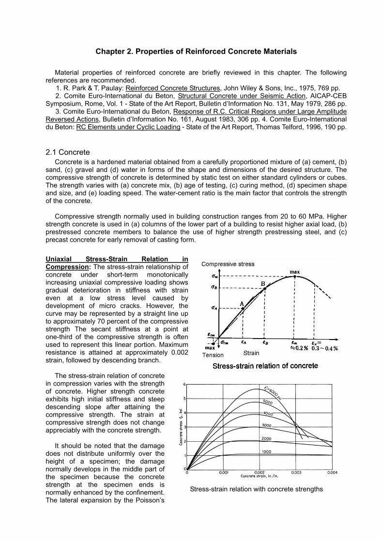
strength concrete is used in (a) columns of the lower part of a building to resist higher axial load, (b) prestressed concrete members to balance the use of higher strength prestressing steel, and (c) precast concrete for early removal of casting form. Uniaxial Stress-Strain Relation in Compression: The stress-strain relationship of concrete under short-term monotonically increasing uniaxial compressive loading shows gradual deterioration in stiffness with strain even at a low stress level caused by development of micro cracks. However, the curve may be represented by a straight line up to approximately 70 percent of the compressive strength The secant stiffness at a point at one-third of the compressive strength is often used to represent this linear portion. Maximum resistance is attained at approximately 0.002 strain, followed by descending branch.

The stress-strain relation of concrete

in compression varies with the strength of concrete. Higher strength concrete exhibits high initial stiffness and steep descending slope after attaining the compressive strength. The strain at compressive strength does not change appreciably with the concrete strength.

It should be noted that the damage

does not distribute uniformly over the height of a specimen; the damage normally develops in the middle part of the specimen because the concrete strength at the specimen ends is normally enhanced by the confinement. The lateral expansion by the Poisson’s

Stress-strain relation with concrete strengths

effect is resisted by the friction between the testing machine. The friction provides confining pressure at the specimen ends, where the strength is enhanced; the damage concentrates in the middle part. For a given stress level, a larger strain is measured in the middle part, and smaller strain near the ends. The strain measurement is affected by the choice of gauge length especially in descending part of the stress-strain curve.

The descending part of the load-deformation relation of a concrete specimen is extremely difficult

to measure because the elastic strain energy stored in the testing machine is released abruptly during the descending part of the test, causing sudden failure of the testing specimen; a stiff loading machine is needed for the purpose.

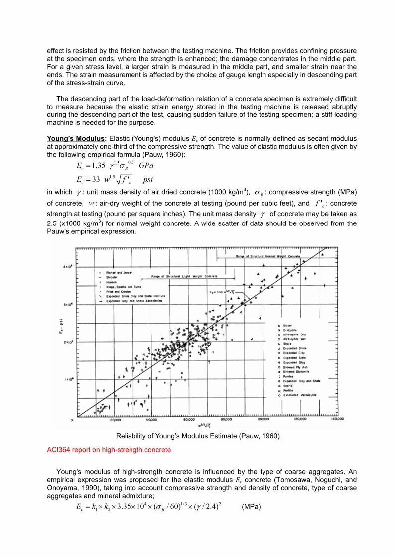
Young’s Modulus: Elastic (Young's) modulus Ec of concrete is normally defined as secant modulus at approximately one-third of the compressive strength. The value of elastic modulus is often given by the following empirical formula (Pauw, 1960):

0.51.5

1.5

1.35

33 'c B

c c

E GPa

E w f psi

γ σ=

=

in which γ : unit mass density of air dried concrete (1000 kg/m3), Bσ : compressive strength (MPa) of concrete, w : air-dry weight of the concrete at testing (pound per cubic feet), and 'cf : concrete strength at testing (pound per square inches). The unit mass density γ of concrete may be taken as 2.5 (x1000 kg/m3) for normal weight concrete. A wide scatter of data should be observed from the Pauw's empirical expression.

ACI364 report on high-strength concrete

Young's modulus of high-strength concrete is influenced by the type of coarse aggregates. An

empirical expression was proposed for the elastic modulus Ec concrete (Tomosawa, Noguchi, and Onoyama, 1990), taking into account compressive strength and density of concrete, type of coarse aggregates and mineral admixture;

4 1/3 21 2 3.35 10 ( / 60) ( / 2.4)c BE k k σ γ= × × × × × (MPa)

Reliability of Young’s Modulus Estimate (Pauw, 1960)

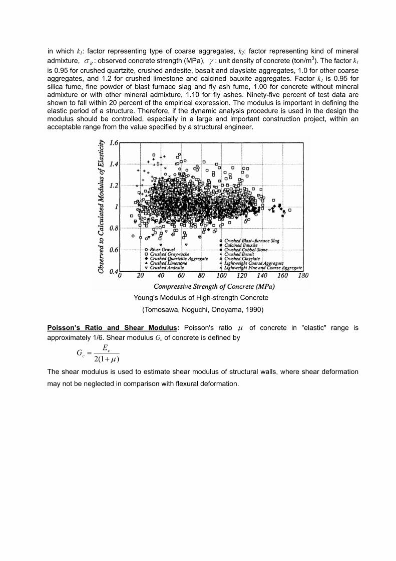
in which k1: factor representing type of coarse aggregates, k2: factor representing kind of mineral admixture, Bσ : observed concrete strength (MPa), γ : unit density of concrete (ton/m3). The factor k1 is 0.95 for crushed quartzite, crushed andesite, basalt and clayslate aggregates, 1.0 for other coarse aggregates, and 1.2 for crushed limestone and calcined bauxite aggregates. Factor k2 is 0.95 for silica fume, fine powder of blast furnace slag and fly ash fume, 1.00 for concrete without mineral admixture or with other mineral admixture, 1.10 for fly ashes. Ninety-five percent of test data are shown to fall within 20 percent of the empirical expression. The modulus is important in defining the elastic period of a structure. Therefore, if the dynamic analysis procedure is used in the design the modulus should be controlled, especially in a large and important construction project, within an acceptable range from the value specified by a structural engineer.

Poisson’s Ratio and Shear Modulus: Poisson's ratio µ of concrete in "elastic" range is approximately 1/6. Shear modulus Gc of concrete is defined by

)1(2 µ+= c

cEG

The shear modulus is used to estimate shear modulus of structural walls, where shear deformation

may not be neglected in comparison with flexural deformation.

Young's Modulus of High-strength Concrete

(Tomosawa, Noguchi, Onoyama, 1990)

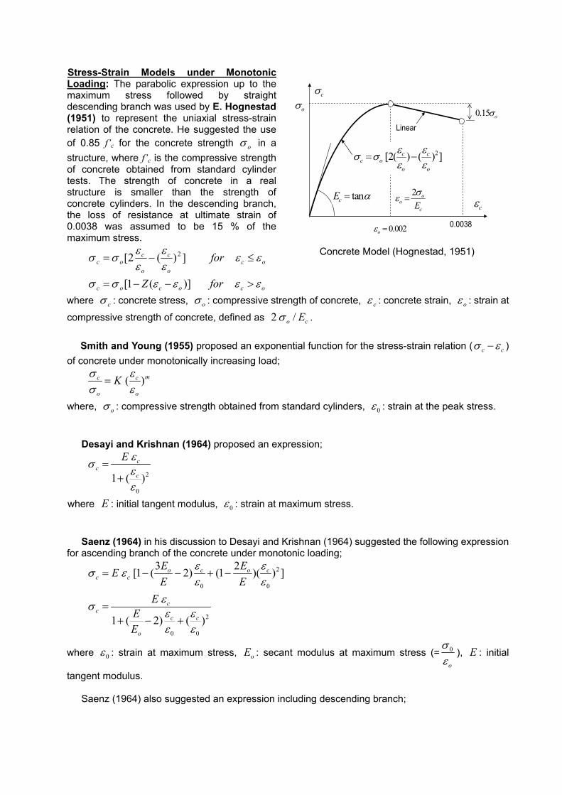
Stress-Strain Models under Monotonic Loading: The parabolic expression up to the maximum stress followed by straight descending branch was used by E. Hognestad (1951) to represent the uniaxial stress-strain relation of the concrete. He suggested the use of 0.85 f’c for the concrete strength oσ in a structure, where f’c is the compressive strength of concrete obtained from standard cylinder tests. The strength of concrete in a real structure is smaller than the strength of concrete cylinders. In the descending branch, the loss of resistance at ultimate strain of 0.0038 was assumed to be 15 % of the maximum stress.

ocococ

oco

c

o

coc

forZ

for

εεεεσσ

εεεε

εεσσ

>−−=

≤−=

)](1[

])(2[ 2

where cσ : concrete stress, oσ : compressive strength of concrete, cε : concrete strain, oε : strain at

compressive strength of concrete, defined as 2 /o cEσ . Smith and Young (1955) proposed an exponential function for the stress-strain relation ( c cσ ε− )

of concrete under monotonically increasing load;

( )mc c

o o

Kσ εσ ε

=

where, oσ : compressive strength obtained from standard cylinders, 0ε : strain at the peak stress. Desayi and Krishnan (1964) proposed an expression;

2

0

1 ( )c

cc

E εσ εε

=+

where E : initial tangent modulus, 0ε : strain at maximum stress. Saenz (1964) in his discussion to Desayi and Krishnan (1964) suggested the following expression

for ascending branch of the concrete under monotonic loading; 2

0 0

2

0 0

3 2[1 ( 2) (1 )( ) ]

1 ( 2) ( )

o c o cc c

cc

c c

o

E EEE EE

EE

ε εσ εε ε

εσ ε εε ε

= − − + −

=+ − +

where 0ε : strain at maximum stress, oE : secant modulus at maximum stress (= 0

o

σε

), E : initial

tangent modulus.

Saenz (1964) also suggested an expression including descending branch;

0.15 oσ

0.0038 0.002oε =

2[2( ) ( ) ]c cc o

o o

ε εσ σε ε

= −

Linear

2 oo

cEσε =

tancE α=

oσcσ

cε

Concrete Model (Hognestad, 1951)

2 3

20 0 0 0 0

02

0 0

1 2 2 1

( 1) 1( 1)

cc

c c c

E

E E E

E f f oE f o

o f

A B C Dwhere

R R R RA B C DE R R RR R ER R R R ER R E εε ε

εσε ε ε

σ σ ε σ εεσ σ

σ ε ε

=+ + +

+ − −= = = − =

−= − = = = =

−

,f fσ ε : stress and strain at failure. The parameters , , ,A B C D were selected to satisfy strains and

stresses at the origin (0,0), maximum stress ( 0 0,ε σ ) and failure point ( ,f fε σ ), initial tangent

stiffness 0

dd ε

σε =

(= E ), slope o

dd ε ε

σε =

(=0.0) at the maximum stress point ( 0 0,ε σ ).

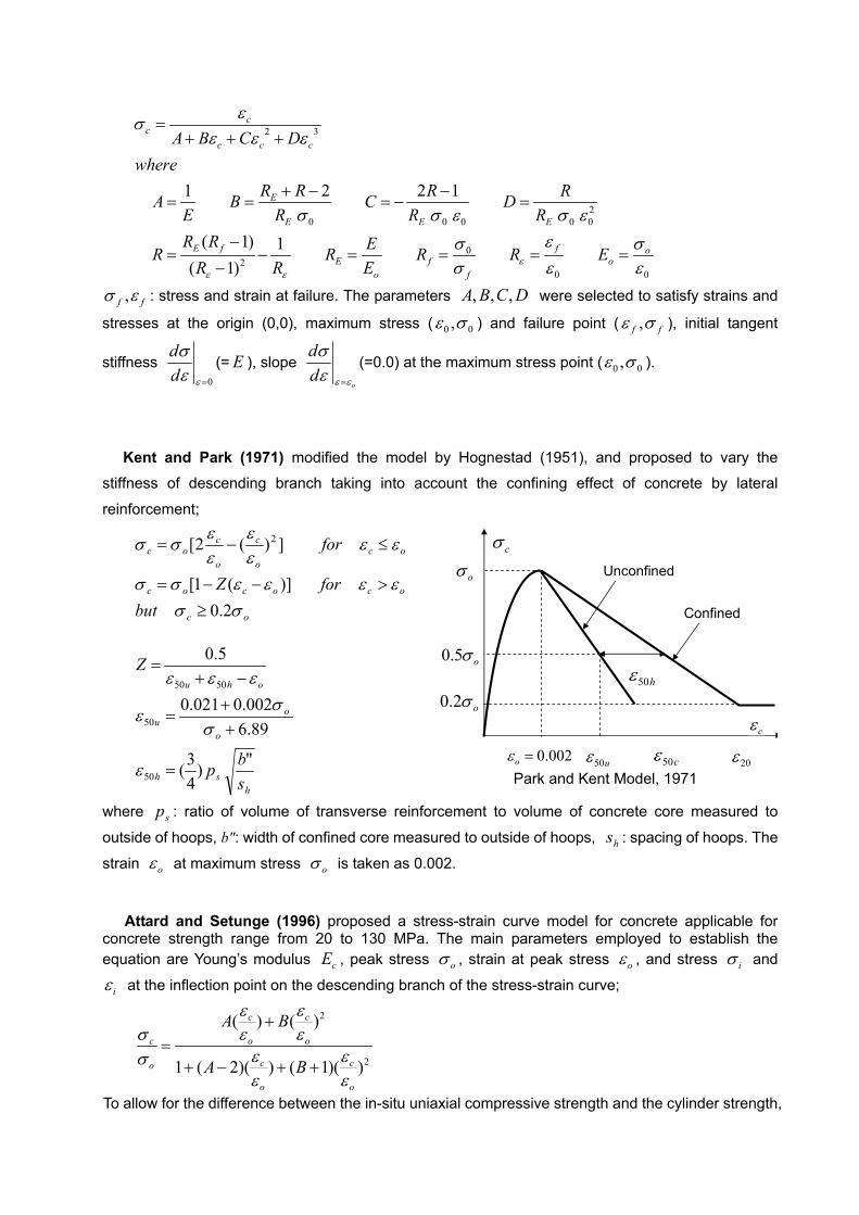
Kent and Park (1971) modified the model by Hognestad (1951), and proposed to vary the

stiffness of descending branch taking into account the confining effect of concrete by lateral

reinforcement;

oc

ocococ

oco

c

o

coc

butforZ

for

σσεεεεσσ

εεεε

εεσσ

2.0)](1[

])(2[ 2

≥>−−=

≤−=

hsh

o

ou

ohu

sbp

Z

")43(

89.6002.0021.0

5.0

50

50

5050

=

++

=

−+=

ε

σσε

εεε

where sp : ratio of volume of transverse reinforcement to volume of concrete core measured to

outside of hoops, b": width of confined core measured to outside of hoops, hs : spacing of hoops. The

strain oε at maximum stress oσ is taken as 0.002.

Attard and Setunge (1996) proposed a stress-strain curve model for concrete applicable for concrete strength range from 20 to 130 MPa. The main parameters employed to establish the equation are Young’s modulus cE , peak stress oσ , strain at peak stress oε , and stress iσ and

iε at the inflection point on the descending branch of the stress-strain curve;

2

2

( ) ( )

1 ( 2)( ) ( 1)( )

c c

c o o

c co

o o

A B

A B

ε εσ ε ε

ε εσε ε

+=

+ − + +

To allow for the difference between the in-situ uniaxial compressive strength and the cylinder strength,

20ε50cε 50uε 0.002oε =

oσ

0.5 oσ

0.2 oσ50hε

cε

cσ

Confined

Unconfined

Park and Kent Model, 1971

the peak stress oσ may be taken as 0.9 times the cylinder strength. For the ascending branch of the stress-strain curve,

2( 1) 10.55

c o

o

EA

AB

εσ

=

−= −

and for descending branch; 2( )

( )0

i i o

o i o i

A

B

σ ε εε ε σ σ

−=

−=

The values , , ,c o i iE ε σ ε may be determined from: 0.52

0.75

4370 ( )

4.11 ( ) /

1.41 0.17 ln( )

2.50 0.30ln( )

c o

o o c

io

o

io

o

EE

σ

ε σσ σσε σε

=

=

= −

= −

where stresses and Young’s modulus are in MPa.

There have been many research works leading to proposals of mathematical or phenomenological models for concrete under short-term uniaxial monotonic loading; e.g., Sargin (1971), Popovics (1970), and Buyukozturk et al. (1971).

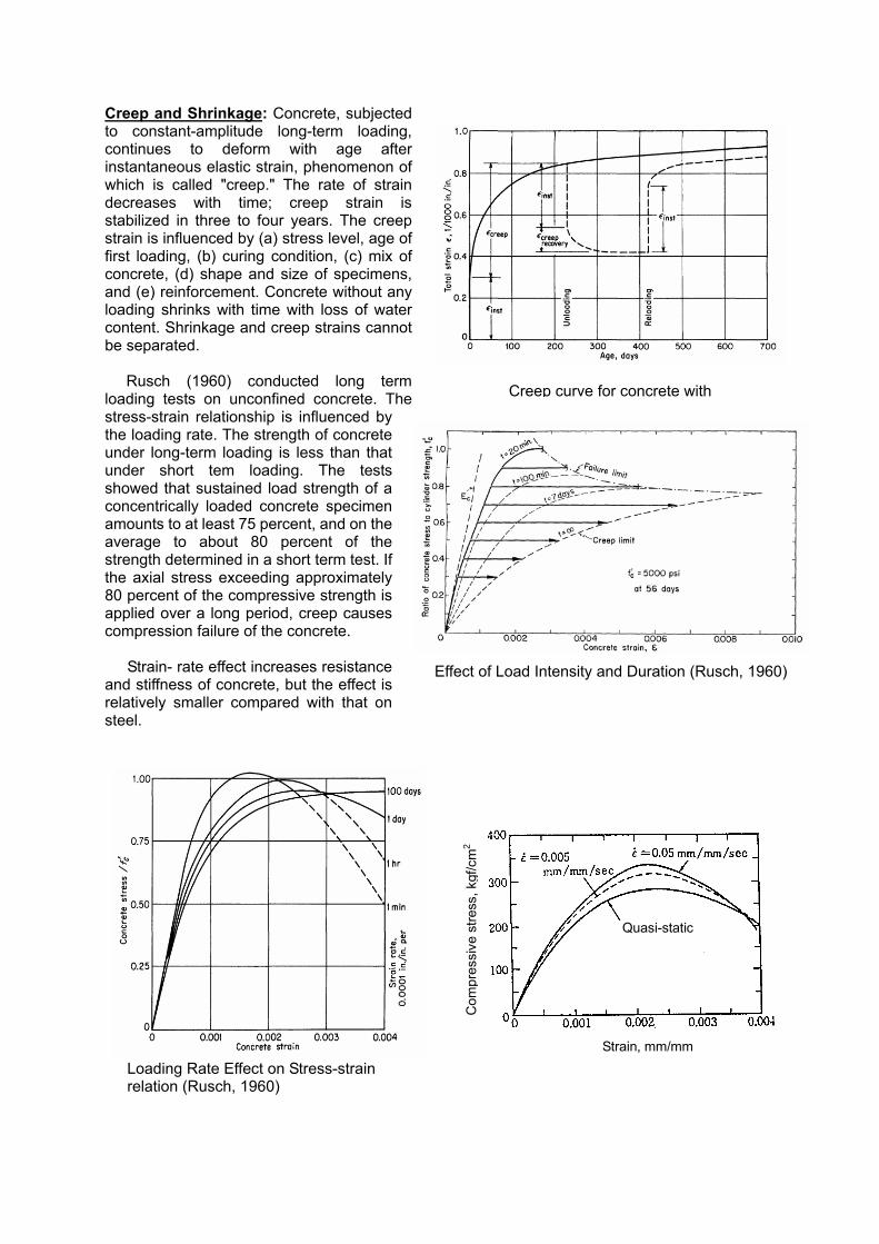
Creep and Shrinkage: Concrete, subjected to constant-amplitude long-term loading, continues to deform with age after instantaneous elastic strain, phenomenon of which is called "creep." The rate of strain decreases with time; creep strain is stabilized in three to four years. The creep strain is influenced by (a) stress level, age of first loading, (b) curing condition, (c) mix of concrete, (d) shape and size of specimens, and (e) reinforcement. Concrete without any loading shrinks with time with loss of water content. Shrinkage and creep strains cannot be separated.

Rusch (1960) conducted long term

loading tests on unconfined concrete. The stress-strain relationship is influenced by the loading rate. The strength of concrete under long-term loading is less than that under short tem loading. The tests showed that sustained load strength of a concentrically loaded concrete specimen amounts to at least 75 percent, and on the average to about 80 percent of the strength determined in a short term test. If the axial stress exceeding approximately 80 percent of the compressive strength is applied over a long period, creep causes compression failure of the concrete.

Strain- rate effect increases resistance

and stiffness of concrete, but the effect is relatively smaller compared with that on steel.

Effect of Load Intensity and Duration (Rusch, 1960)

Strain, mm/mm

Com

pres

sive

stre

ss, k

gf/c

m2

Quasi-static

Loading Rate Effect on Stress-strain relation (Rusch, 1960)

Creep curve for concrete with

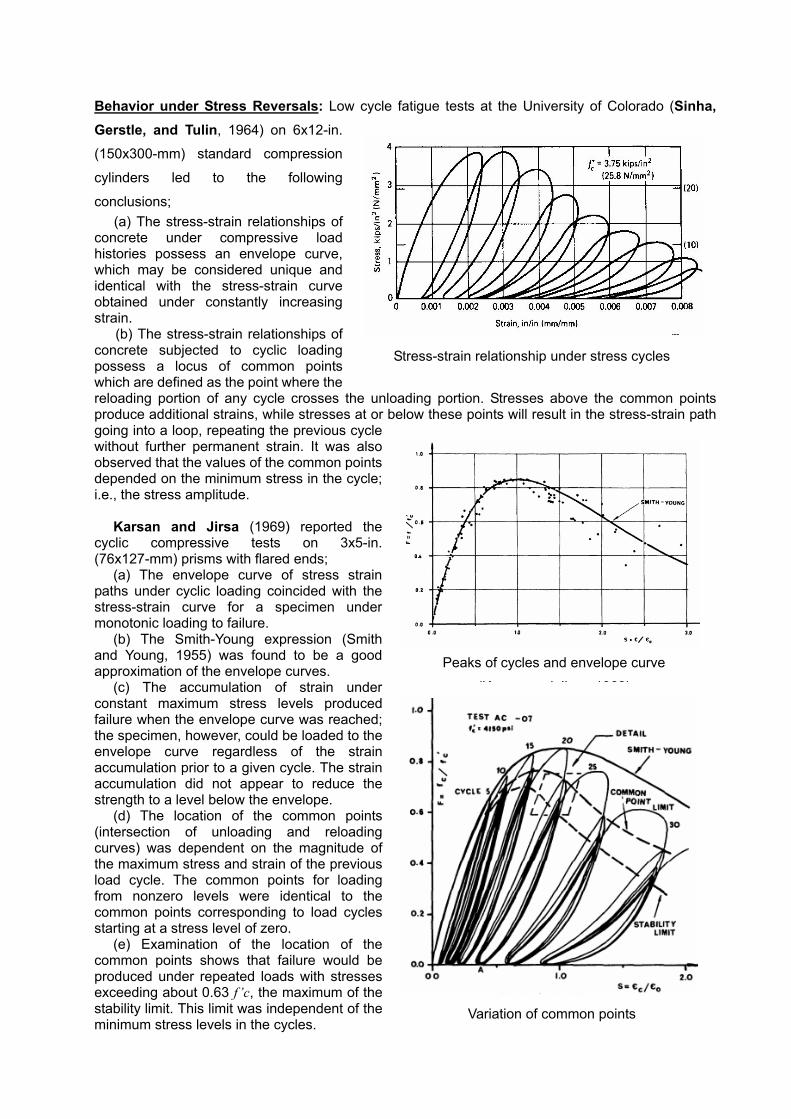
Behavior under Stress Reversals: Low cycle fatigue tests at the University of Colorado (Sinha, Gerstle, and Tulin, 1964) on 6x12-in.

(150x300-mm) standard compression

cylinders led to the following

conclusions; (a) The stress-strain relationships of

concrete under compressive load histories possess an envelope curve, which may be considered unique and identical with the stress-strain curve obtained under constantly increasing strain.

(b) The stress-strain relationships of concrete subjected to cyclic loading possess a locus of common points which are defined as the point where the reloading portion of any cycle crosses the unloading portion. Stresses above the common points produce additional strains, while stresses at or below these points will result in the stress-strain path going into a loop, repeating the previous cycle without further permanent strain. It was also observed that the values of the common points depended on the minimum stress in the cycle; i.e., the stress amplitude.

Karsan and Jirsa (1969) reported the cyclic compressive tests on 3x5-in. (76x127-mm) prisms with flared ends;

(a) The envelope curve of stress strain paths under cyclic loading coincided with the stress-strain curve for a specimen under monotonic loading to failure.

(b) The Smith-Young expression (Smith and Young, 1955) was found to be a good approximation of the envelope curves.

(c) The accumulation of strain under constant maximum stress levels produced failure when the envelope curve was reached; the specimen, however, could be loaded to the envelope curve regardless of the strain accumulation prior to a given cycle. The strain accumulation did not appear to reduce the strength to a level below the envelope.

(d) The location of the common points (intersection of unloading and reloading curves) was dependent on the magnitude of the maximum stress and strain of the previous load cycle. The common points for loading from nonzero levels were identical to the common points corresponding to load cycles starting at a stress level of zero.

(e) Examination of the location of the common points shows that failure would be produced under repeated loads with stresses exceeding about 0.63 f ’c, the maximum of the stability limit. This limit was independent of the minimum stress levels in the cycles.

Stress-strain relationship under stress cycles

Peaks of cycles and envelope curve

(K d Ji 1969)

Variation of common points

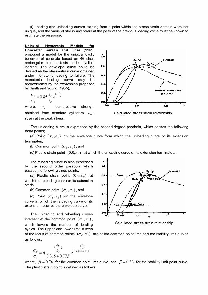
(f) Loading and unloading curves starting from a point within the stress-strain domain were not unique, and the value of stress and strain at the peak of the previous loading cycle must be known to estimate the response. Uniaxial Hysteresis Models for Concrete: Karsan and Jirsa (1969) proposed a model for the uniaxial cyclic behavior of concrete based on 46 short rectangular column tests under cyclical loading. The envelope curve could be defined as the stress-strain curve obtained under monotonic loading to failure. The monotonic loading curve may be approximated by the expression proposed by Smith and Young (1955);

(1 )0.85

c

oc c

o o

eεεσ ε

σ ε

−

=

where, oσ : compressive strength

obtained from standard cylinders, oε : strain at the peak stress.

The unloading curve is expressed by the second-degree parabola, which passes the following three points;

(a) Point ( , )E Eσ ε on the envelope curve from which the unloading curve or its extension terminates,

(b) Common point ( , )C Cσ ε , and

(c) Plastic strain point (0.0, )Pε at which the unloading curve or its extension terminates.

The reloading curve is also expressed by the second order parabola which passes the following three points;

(a) Plastic strain point (0.0, )Pε at which the reloading curve or its extension starts,

(b) Common point ( , )C Cσ ε , and

(c) Point ( , )E Eσ ε on the envelope curve at which the reloading curve or its extension reaches the envelope curve.

The unloading and reloading curves intersect at the common point ( , )C Cσ ε , which lowers the number of loading cycles. The upper and lower limit curves of the locus of common points ( , )C Cσ ε are called common point limit and the stability limit curves as follows;

( )[1 ]

0.315 0.77

( )

0.315 0.77

C

oC

C o

o

e

εε

β

εσ εβσ β

−+=

+

where, 0.76β = for the common point limit curve, and 0.63β = for the stability limit point curve. The plastic strain point is defined as follows;

Calculated stress strain relationship

Calculated stress-strain relationship

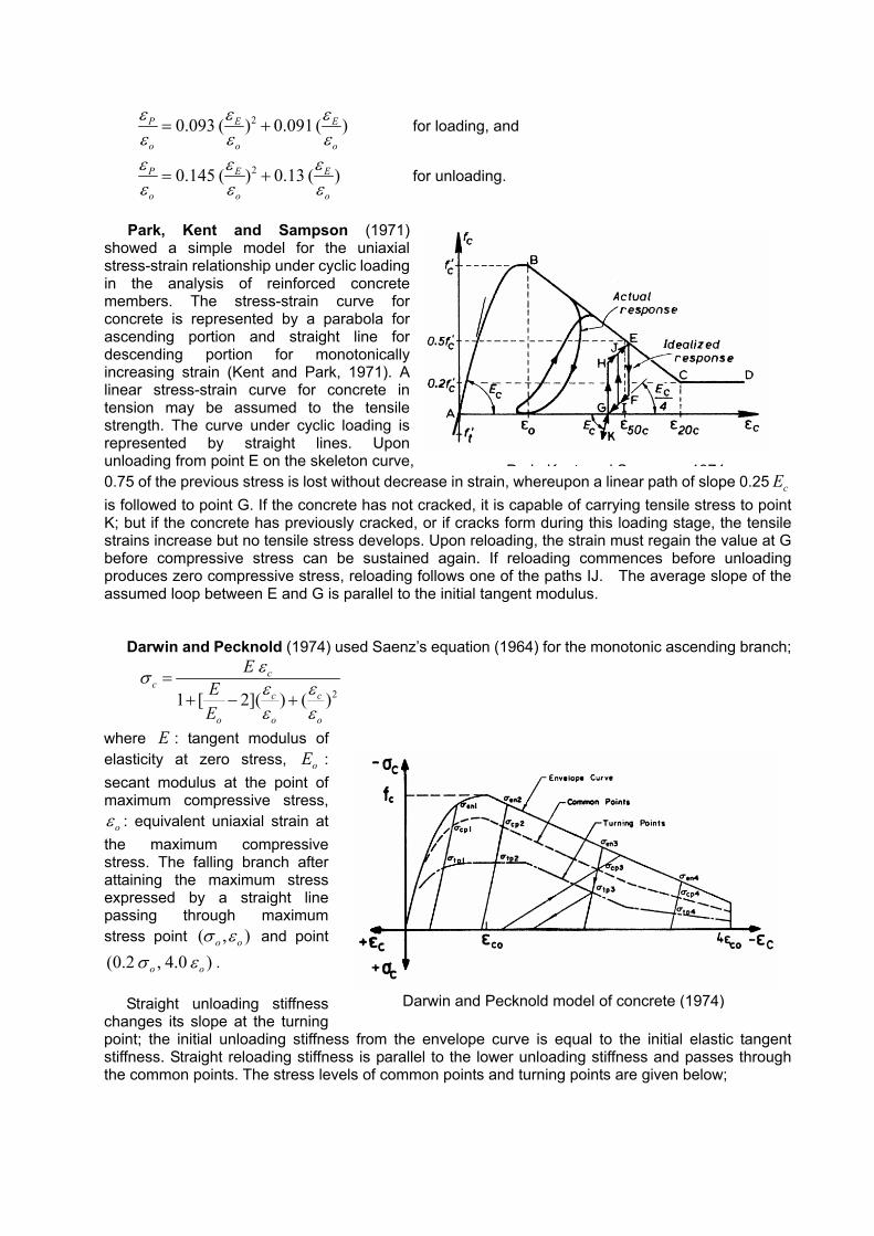
20.093 ( ) 0.091 ( )P E E

o o o

ε ε εε ε ε

= + for loading, and

20.145 ( ) 0.13 ( )P E E

o o o

ε ε εε ε ε

= + for unloading.

Park, Kent and Sampson (1971)

showed a simple model for the uniaxial stress-strain relationship under cyclic loading in the analysis of reinforced concrete members. The stress-strain curve for concrete is represented by a parabola for ascending portion and straight line for descending portion for monotonically increasing strain (Kent and Park, 1971). A linear stress-strain curve for concrete in tension may be assumed to the tensile strength. The curve under cyclic loading is represented by straight lines. Upon unloading from point E on the skeleton curve, 0.75 of the previous stress is lost without decrease in strain, whereupon a linear path of slope 0.25 cE is followed to point G. If the concrete has not cracked, it is capable of carrying tensile stress to point K; but if the concrete has previously cracked, or if cracks form during this loading stage, the tensile strains increase but no tensile stress develops. Upon reloading, the strain must regain the value at G before compressive stress can be sustained again. If reloading commences before unloading produces zero compressive stress, reloading follows one of the paths IJ. The average slope of the assumed loop between E and G is parallel to the initial tangent modulus.

Darwin and Pecknold (1974) used Saenz’s equation (1964) for the monotonic ascending branch;

21 [ 2]( ) ( )c

cc c

o o o

EEE

εσ ε εε ε

=+ − +

where E : tangent modulus of elasticity at zero stress, oE : secant modulus at the point of maximum compressive stress, oε : equivalent uniaxial strain at

the maximum compressive stress. The falling branch after attaining the maximum stress expressed by a straight line passing through maximum stress point ( , )o oσ ε and point

(0.2 , 4.0 )o oσ ε .

Straight unloading stiffness changes its slope at the turning point; the initial unloading stiffness from the envelope curve is equal to the initial elastic tangent stiffness. Straight reloading stiffness is parallel to the lower unloading stiffness and passes through the common points. The stress levels of common points and turning points are given below;

P k K t d S 1974

Darwin and Pecknold model of concrete (1974)

Region 1: 1 1

1 1

5612

cp en

tp en

σ σ

σ σ

=

=

Region 2: 2 2 2

2 2

1 1min{ , }6 6

1 1min{ , }2 2

cp en en B

tp en B

σ σ σ σ

σ σ σ

= −

=

Region 3:

3 3

3 3 3 3

3

162( )

13

cp en B

tp en en cp

en B

σ σ σ

σ σ σ σ

σ σ

= −

= − −

= −

Region 4: 4 4

4

23

13

cp en

tp en

σ σ

σ σ

=

=

Other models can be found in literatures by Blakely (1973) and Aoyama (1973).

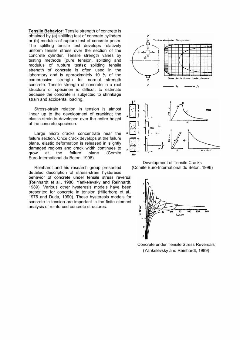
Tensile Behavior: Tensile strength of concrete is obtained by (a) splitting test of concrete cylinders or (b) modulus of rupture test of concrete prism. The splitting tensile test develops relatively uniform tensile stress over the section of the concrete cylinder. Tensile strength varies by testing methods (pure tension, splitting and modulus of rupture tests); splitting tensile strength of concrete is often used in the laboratory and is approximately 10 % of the compressive strength for normal strength concrete. Tensile strength of concrete in a real structure or specimen is difficult to estimate because the concrete is subjected to shrinkage strain and accidental loading.

Stress-strain relation in tension is almost

linear up to the development of cracking; the elastic strain is developed over the entire height of the concrete specimen.

Large micro cracks concentrate near the

failure section. Once crack develops at the failure plane, elastic deformation is released in slightly damaged regions and crack width continues to grow at the failure plane (Comite Euro-International du Beton, 1996).

Reinhardt and his research group presented

detailed description of stress-strain hysteresis behavior of concrete under tensile stress reversal (Reinhardt et al., 1986, Yankelevsky and Reinhardt, 1989). Various other hysteresis models have been presented for concrete in tension (Hillerborg et al., 1976 and Duda, 1990). These hysteresis models for concrete in tension are important in the finite element analysis of reinforced concrete structures.

Development of Tensile Cracks (Comite Euro-International du Beton, 1996)

Concrete under Tensile Stress Reversals

(Yankelevsky and Reinhardt, 1989)

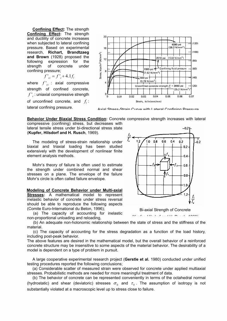
Confining Effect: The strength Confining Effect: The strength and ductility of concrete increases when subjected to lateral confining pressure. Based on experimental research, Richart, Brandtzaeg and Brown (1928) proposed the following expression for the strength of concrete under confining pressure; ' ' 4.1cc c lf f f= +

where 'ccf : axial compressive strength of confined concrete,

'cf : uniaxial compressive strength

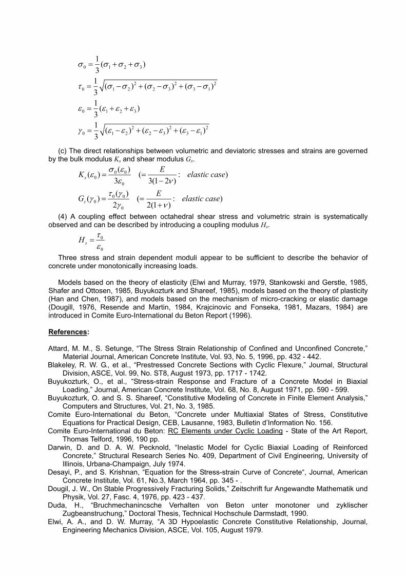
of unconfined concrete, and lf : lateral confining pressure. Behavior Under Biaxial Stress Condition: Concrete compressive strength increases with lateral compressive (confining) stress, but decreases with lateral tensile stress under bi-directional stress state (Kupfer, Hilsdorf and H. Rusch, 1969).

The modeling of stress-strain relationship under biaxial and triaxial loading has been studied extensively with the development of nonlinear finite element analysis methods.

Mohr’s theory of failure is often used to estimate

the strength under combined normal and shear stresses on a plane. The envelope of the failure Mohr’s circle is often called failure envelope. Modeling of Concrete Behavior under Multi-axial Stresses: A mathematical model to represent inelastic behavior of concrete under stress reversal should be able to reproduce the following aspects (Comite Euro-International du Beton, 1996);

(a) The capacity of accounting for inelastic non-proportional unloading and reloading,

(b) An adequate non-holonomic relationship between the state of stress and the stiffness of the material.

(c) The capacity of accounting for the stress degradation as a function of the load history, including post-peak behavior. The above features are desired in the mathematical model, but the overall behavior of a reinforced concrete structure may be insensitive to some aspects of the material behavior. The desirability of a model is dependent on a type of problem in pursuit.

A large cooperative experimental research project (Gerstle et al. 1980) conducted under unified testing procedures reported the following conclusions;

(a) Considerable scatter of measured strain were observed for concrete under applied multiaxial stresses. Probabilistic methods are needed for more meaningful treatment of data.

(b) The behavior of concrete can be represented conveniently in terms of the octahedral normal (hydrostatic) and shear (deviatoric) stresses 0σ and 0τ . The assumption of isotropy is not substantially violated at a macroscopic level up to stress close to failure.

Bi-axial Strength of Concrete

(Kupfer Hilsdorf and H Rusch 1969)

Axial Stress-Strain Curve with Lateral Confining Pressure

0 1 2 3

2 2 20 1 2 2 3 3 1

0 1 2 3

2 2 20 1 2 2 3 3 1

1 ( )31 ( ) ( ) ( )31 ( )31 ( ) ( ) ( )3

σ σ σ σ

τ σ σ σ σ σ σ

ε ε ε ε

γ ε ε ε ε ε ε

= + +

= − + − + −

= + +

= − + − + −

(c) The direct relationships between volumetric and deviatoric stresses and strains are governed by the bulk modulus Ks and shear modulus Gs.

0 00

0

0 00

0

( )( ) ( : )3 3(1 2 )( )( ) ( : )

2 2(1 )

s

s

EK elastic case

EG elastic case

σ εεε ν

τ γγγ ν

= =−

= =+

(4) A coupling effect between octahedral shear stress and volumetric strain is systematically observed and can be described by introducing a coupling modulus Hs.

0

0sH

τε

=

Three stress and strain dependent moduli appear to be sufficient to describe the behavior of concrete under monotonically increasing loads.

Models based on the theory of elasticity (Elwi and Murray, 1979, Stankowski and Gerstle, 1985,

Shafer and Ottosen, 1985, Buyukozturk and Shareef, 1985), models based on the theory of plasticity (Han and Chen, 1987), and models based on the mechanism of micro-cracking or elastic damage (Dougill, 1976, Resende and Martin, 1984, Krajcinovic and Fonseka, 1981, Mazars, 1984) are introduced in Comite Euro-International du Beton Report (1996). References: Attard, M. M., S. Setunge, “The Stress Strain Relationship of Confined and Unconfined Concrete,”

Material Journal, American Concrete Institute, Vol. 93, No. 5, 1996, pp. 432 - 442. Blakeley, R. W. G., et al., “Prestressed Concrete Sections with Cyclic Flexure,” Journal, Structural

Division, ASCE, Vol. 99, No. ST8, August 1973, pp. 1717 - 1742. Buyukozturk, O., et al., “Stress-strain Response and Fracture of a Concrete Model in Biaxial

Loading,” Journal, American Concrete Institute, Vol. 68, No. 8, August 1971, pp. 590 - 599. Buyukozturk, O. and S. S. Shareef, “Constitutive Modeling of Concrete in Finite Element Analysis,”

Computers and Structures, Vol. 21, No. 3, 1985. Comite Euro-International du Beton, “Concrete under Multiaxial States of Stress, Constitutive

Equations for Practical Design, CEB, Lausanne, 1983, Bulletin d’Information No. 156. Comite Euro-International du Beton: RC Elements under Cyclic Loading - State of the Art Report,

Thomas Telford, 1996, 190 pp. Darwin, D. and D. A. W. Pecknold, “Inelastic Model for Cyclic Biaxial Loading of Reinforced

Concrete,” Structural Research Series No. 409, Department of Civil Engineering, University of Illinois, Urbana-Champaign, July 1974.

Desayi, P., and S. Krishnan, “Equation for the Stress-strain Curve of Concrete“, Journal, American Concrete Institute, Vol. 61, No.3, March 1964, pp. 345 - .

Dougil, J. W., On Stable Progressively Fracturing Solids,” Zeitschrift fur Angewandte Mathematik und Physik, Vol. 27, Fasc. 4, 1976, pp. 423 - 437.

Duda, H., “Bruchmechanincsche Verhalten von Beton unter monotoner und zyklischer Zugbeanstruchung,” Doctoral Thesis, Technical Hochschule Darmstadt, 1990.

Elwi, A. A., and D. W. Murray, “A 3D Hypoelastic Concrete Constitutive Relationship, Journal, Engineering Mechanics Division, ASCE, Vol. 105, August 1979.

Gerstle, K. H., H. Aschl, R. Bellotti, P. Bertacchi, M. D. Kotsovos, H. Y. Ko, D. Linse, J. B. Newman, P. Rossi, G. Schickert, M. A. Taylor, L. A. Traina, H. Winkler and R. M. Zimmerman, “Behavior of Concrete under Multiaxial Stress States,” Journal, Engineering Mechanics, ASCE, Vol. 106, No. 6, December 1980, pp. 1383 - 1404.

Han, D. J., and W. F. Chen, “A Nonuniform Hardening Plasticity Model for Concrete Materials,” Journal, Mech. Mat., Vol. 4, 1985.

Hillerborg, A. et al., “Analysis of Crack Formation and Crack Growth in concrete by Means of Fracture Mechanics and Finite Elements,” Cement and Concrete Research, Vol. 6, 1976, pp. 773 - 782.

Hognestad, E., "A Study of Combined Bending and Axial Load in Reinforced Concrete Members," Bulletin No. 399, Engineering Experimental Station, University of Illinois, 1951.

Karsan, I. D., and J. O. Jirsa, “Behavior of Concrete under Compressive Loadings,” Journal, Structures Division, ASCE, Vol. 95, No. ST12, December 1969, pp. 2543 - 2563.

Kent, D. C., and R. Park, "Flexural Members with Confined Concrete," Journal, Structural Division, ASCE, Vol. 97, ST 7, July 1971, pp. 1969-1990.

Krajcinovic, D., and G. U. Fonseka, “The Continuous Damage Theory of Brittle Materials,” Journal, Applied Mechanics, ASME, Vol. 48, 1981.

Kupfer, H., H. K. Hilsdorf, and H. Rusch, "Behavior of Concrete Under Bi-axial Stress," Journal, American Concrete Institute, Vol. 66, No. 8, pp. 656-666, August 1969.

Mander, J. M., N. M. Priestley and R. Park, “Theoretical Stress-Strain Model for Confined Concrete,” Journal, Structural Division, ASCE, Vol. 114, No. 8, 1988, pp. 1804 - 1826.

Mazars, J., “Description of the Multiaxial Behavior of Concrete under Multiaxial Conditions,” INSA-OPS Toulouse, May 1984.

Park, R., and T. Paulay, Reinforced Concrete Structures, John Wiley & Sons, 1975, 769 pp. Pauw, A., "Static Modulus of Elasticity of Concrete as Affected by Density," Journal, American

Concrete Institute, No. 57, No. 6, December 1960, pp. 679-687. Popovics, S., “Stress-strain Relations for Concrete under Compression,” Journal, American Concrete

Institute, Vol. 67, No. 3, March 1970, pp. 243 - 248. Popovics, S., “A Review of Stress-Strain Curve of Concrete,” Cement and Concrete Research, Vo. 3,

No. 4, September 1973, pp. 583 - 599. Reinhardt, H. W. et al., “Tensile Tests and Failure Analysis of Concrete,” Journal, Structural

Engineering, ASCE, Vol. 112, No. 11, November 1986, pp. 2462 - 2477. Resende, L., and J. B. Martin, “A Progressive Damage Continuum Model for Granular Materials,”

Comp. Meth. Appl. Mech. Engng, Vol. 42, 1984. Richart, F. E., A. Brandtzaeg, and R. L. Brown, “A Study of the Failure of Concrete Under Combined

Compressive Stresses,” University of Illinois Engineering Experimental Station, Bulletin No. 185, 1928, 104 pp.

Rusch, H., “Researches Toward a General Flexural Theory for Structural Concrete,” Journal, American Concrete Institute, Vol. 57, No. 1, July 1960, pp. 1 - 28.

Saenz, L. P., “Discussion of the paper by Desayi, P., and S. Krishnan entitled ‘Equation for the Stress-strain Curve of Concrete’,” Journal, American Concrete Institute, Vol. 61, No. 9, September 1964, pp. 1229 - 1235.

Sargin, M., “Stress-strain Relationships for Concrete and the Analysis of Structural Concrete Sections,” Study No. 4, Solid Mechanics Division, University of Waterloo, Ontario, 1971, 167 pp.

Sinha, B. P., K. H. Gerstle, and L. G. Tulin, "Stress-Strain Relationships for Concrete Under Cyclic Loading," Journal, American Concrete Institute, Vol. 61, No. 2, pp. 195-211, February 1964.

Smith, G. M., and L. E. Young, “Ultimate Theory in Flexure by Exponential Function,” Journal, American Concrete Institute, Vol. 52, No. 3, November 1955, pp. 349 - 359.

Shafer, G. S., and N. S. Ottosen, “An Invariant-based Constitutive Model, Structural Research Series No. 8506, Department of Civil Environmental and Architectural Engineering, University of Colorado, Boulder, 1985.

Stankowski, T., and K. H. Gerstle, “Simple Formulation of Concrete Behavior under Multiaxial Load Histories,” Journal, American Concrete Institute, Vol. 82, No. 2., March-April 1985.

Tomosawa, F., T. Noguchi, and K. Onoyama, "Investigation on Fundamental Mechanical Properties of High-strength and Super High Strength Concrete (in Japanese)," Summaries of Technical Papers of Annual Meeting of Architectural Institute of Japan, Vol. A, 1990, pp. 497-498.

Yankelevsky, D. Z. and H. W. Reinhardt, “Uniaxial Behavior of Concrete in Cyclic Tension,” Journal, Structural Engineering, ASCE, Vol. 115, No. 1, 1989, pp. 166-182.

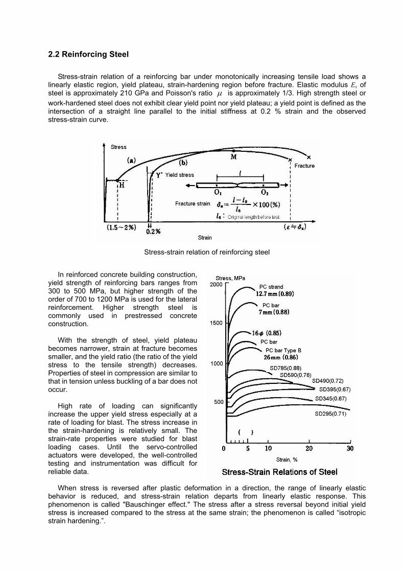
2.2 Reinforcing Steel

Stress-strain relation of a reinforcing bar under monotonically increasing tensile load shows a linearly elastic region, yield plateau, strain-hardening region before fracture. Elastic modulus Es of steel is approximately 210 GPa and Poisson's ratio µ is approximately 1/3. High strength steel or work-hardened steel does not exhibit clear yield point nor yield plateau; a yield point is defined as the intersection of a straight line parallel to the initial stiffness at 0.2 % strain and the observed stress-strain curve.

Stress-strain relation of reinforcing steel

In reinforced concrete building construction,

yield strength of reinforcing bars ranges from 300 to 500 MPa, but higher strength of the order of 700 to 1200 MPa is used for the lateral reinforcement. Higher strength steel is commonly used in prestressed concrete construction.

With the strength of steel, yield plateau

becomes narrower, strain at fracture becomes smaller, and the yield ratio (the ratio of the yield stress to the tensile strength) decreases. Properties of steel in compression are similar to that in tension unless buckling of a bar does not occur.

High rate of loading can significantly

increase the upper yield stress especially at a rate of loading for blast. The stress increase in the strain-hardening is relatively small. The strain-rate properties were studied for blast loading cases. Until the servo-controlled actuators were developed, the well-controlled testing and instrumentation was difficult for reliable data.

When stress is reversed after plastic deformation in a direction, the range of linearly elastic behavior is reduced, and stress-strain relation departs from linearly elastic response. This phenomenon is called "Bauschinger effect." The stress after a stress reversal beyond initial yield stress is increased compared to the stress at the same strain; the phenomenon is called “isotropic strain hardening.”.

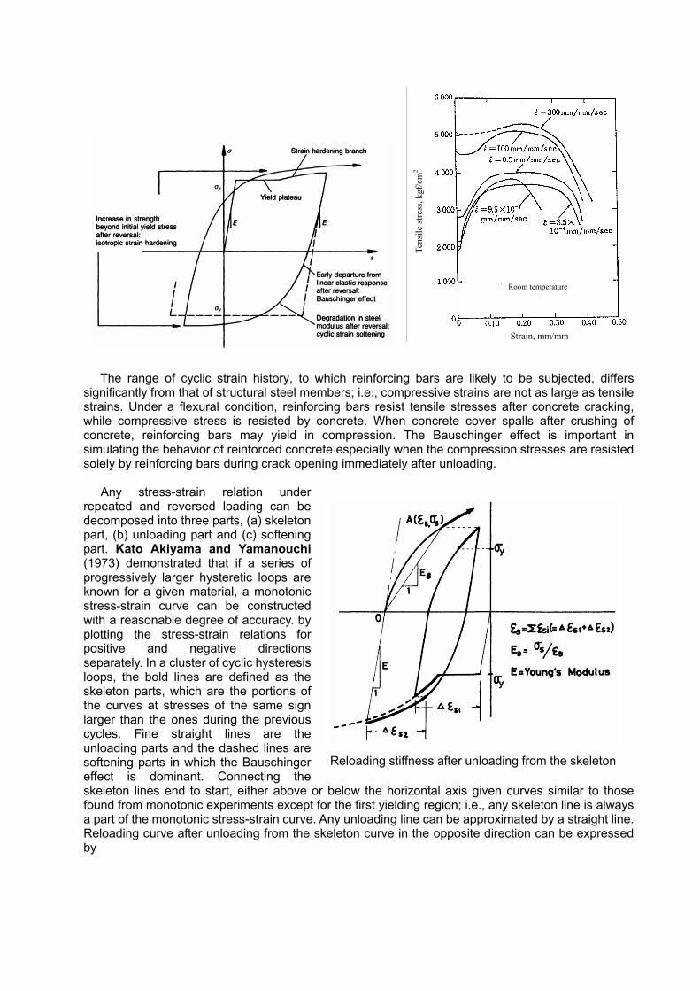
The range of cyclic strain history, to which reinforcing bars are likely to be subjected, differs

significantly from that of structural steel members; i.e., compressive strains are not as large as tensile strains. Under a flexural condition, reinforcing bars resist tensile stresses after concrete cracking, while compressive stress is resisted by concrete. When concrete cover spalls after crushing of concrete, reinforcing bars may yield in compression. The Bauschinger effect is important in simulating the behavior of reinforced concrete especially when the compression stresses are resisted solely by reinforcing bars during crack opening immediately after unloading.

Any stress-strain relation under

repeated and reversed loading can be decomposed into three parts, (a) skeleton part, (b) unloading part and (c) softening part. Kato Akiyama and Yamanouchi (1973) demonstrated that if a series of progressively larger hysteretic loops are known for a given material, a monotonic stress-strain curve can be constructed with a reasonable degree of accuracy. by plotting the stress-strain relations for positive and negative directions separately. In a cluster of cyclic hysteresis loops, the bold lines are defined as the skeleton parts, which are the portions of the curves at stresses of the same sign larger than the ones during the previous cycles. Fine straight lines are the unloading parts and the dashed lines are softening parts in which the Bauschinger effect is dominant. Connecting the skeleton lines end to start, either above or below the horizontal axis given curves similar to those found from monotonic experiments except for the first yielding region; i.e., any skeleton line is always a part of the monotonic stress-strain curve. Any unloading line can be approximated by a straight line. Reloading curve after unloading from the skeleton curve in the opposite direction can be expressed by

Reloading stiffness after unloading from the skeleton

Tens

ile st

ress

, kgf

/cm

2

Room temperature

Strain, mm/mm

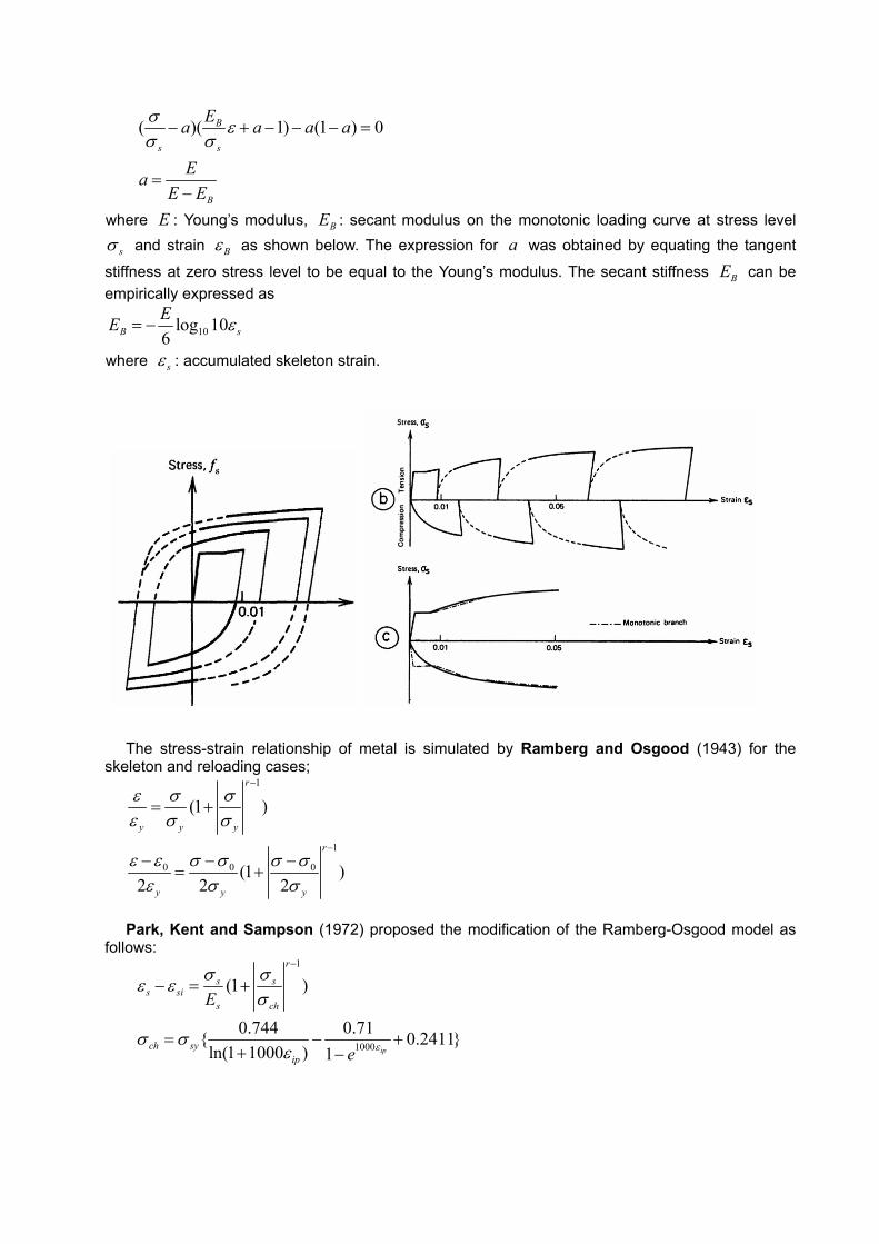
( )( 1) (1 ) 0B

s s

B

Ea a a a

EaE E

σ εσ σ

− + − − − =

=−

where E : Young’s modulus, BE : secant modulus on the monotonic loading curve at stress level

sσ and strain Bε as shown below. The expression for a was obtained by equating the tangent

stiffness at zero stress level to be equal to the Young’s modulus. The secant stiffness BE can be empirically expressed as

10log 106B sEE ε= −

where sε : accumulated skeleton strain.

The stress-strain relationship of metal is simulated by Ramberg and Osgood (1943) for the

skeleton and reloading cases; 1

1

0 0 0

(1 )

(1 )2 2 2

r

y y y

r

y y y

ε σ σε σ σ

ε ε σ σ σ σε σ σ

−

−

= +

− − −= +

Park, Kent and Sampson (1972) proposed the modification of the Ramberg-Osgood model as

follows: 1

1000

(1 )

0.744 0.71{ 0.2411}ln(1 1000 ) 1 ip

r

s ss si

s ch

ch syip

E

e ε

σ σε εσ

σ σε

−

− = +

= − ++ −

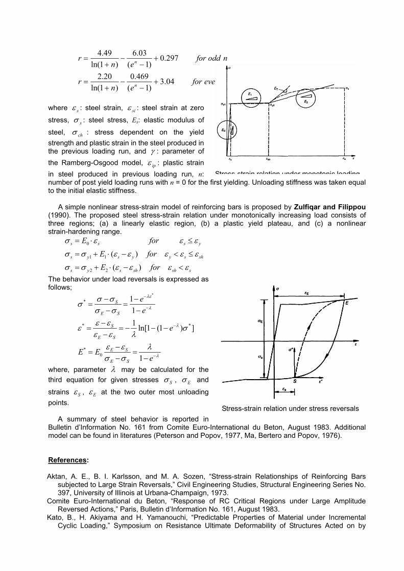
nevenforen

r

noddforen

r

n

n

04.3)1(

469.0)1ln(

20.2

297.0)1(

03.6)1ln(

49.4

+−

−+

=

+−

−+

=

where sε : steel strain, siε : steel strain at zero

stress, sσ : steel stress, Es: elastic modulus of

steel, chσ : stress dependent on the yield strength and plastic strain in the steel produced in the previous loading run, and γ : parameter of the Ramberg-Osgood model, ipε : plastic strain in steel produced in previous loading run, n: number of post yield loading runs with n = 0 for the first yielding. Unloading stiffness was taken equal to the initial elastic stiffness.

A simple nonlinear stress-strain model of reinforcing bars is proposed by Zulfiqar and Filippou (1990). The proposed steel stress-strain relation under monotonically increasing load consists of three regions; (a) a linearly elastic region, (b) a plastic yield plateau, and (c) a nonlinear strain-hardening range.

0

1 1

2 2

( )

( )

s s s y

s y s y y s sh

s y s sh sh s

E forE forE for

σ ε ε ε

σ σ ε ε ε ε ε

σ σ ε ε ε ε

= ⋅ ≤

= + ⋅ − < ≤

= + ⋅ − <

The behavior under load reversals is expressed as follows;

*

*

* *

*0

111 ln[1 (1 ) ]

1

S

E S

S

E S

E S

E S

ee

e

E Ee

λε

λ

λ

λ

σ σσσ σε εε σε ε λ

ε ε λσ σ

−

−

−

−

− −= =

− −−

= = − − −−

−= =

− −

where, parameter λ may be calculated for the third equation for given stresses Sσ , Eσ and

strains Sε , Eε at the two outer most unloading points.

A summary of steel behavior is reported in Bulletin d’Information No. 161 from Comite Euro-International du Beton, August 1983. Additional model can be found in literatures (Peterson and Popov, 1977, Ma, Bertero and Popov, 1976). References: Aktan, A. E., B. I. Karlsson, and M. A. Sozen, “Stress-strain Relationships of Reinforcing Bars

subjected to Large Strain Reversals,” Civil Engineering Studies, Structural Engineering Series No. 397, University of Illinois at Urbana-Champaign, 1973.

Comite Euro-International du Beton, “Response of RC Critical Regions under Large Amplitude Reversed Actions,” Paris, Bulletin d’Information No. 161, August 1983.

Kato, B., H. Akiyama and H. Yamanouchi, “Predictable Properties of Material under Incremental Cyclic Loading,” Symposium on Resistance Ultimate Deformability of Structures Acted on by

Stress strain relation under monotonic loading

Stress-strain relation under stress reversals

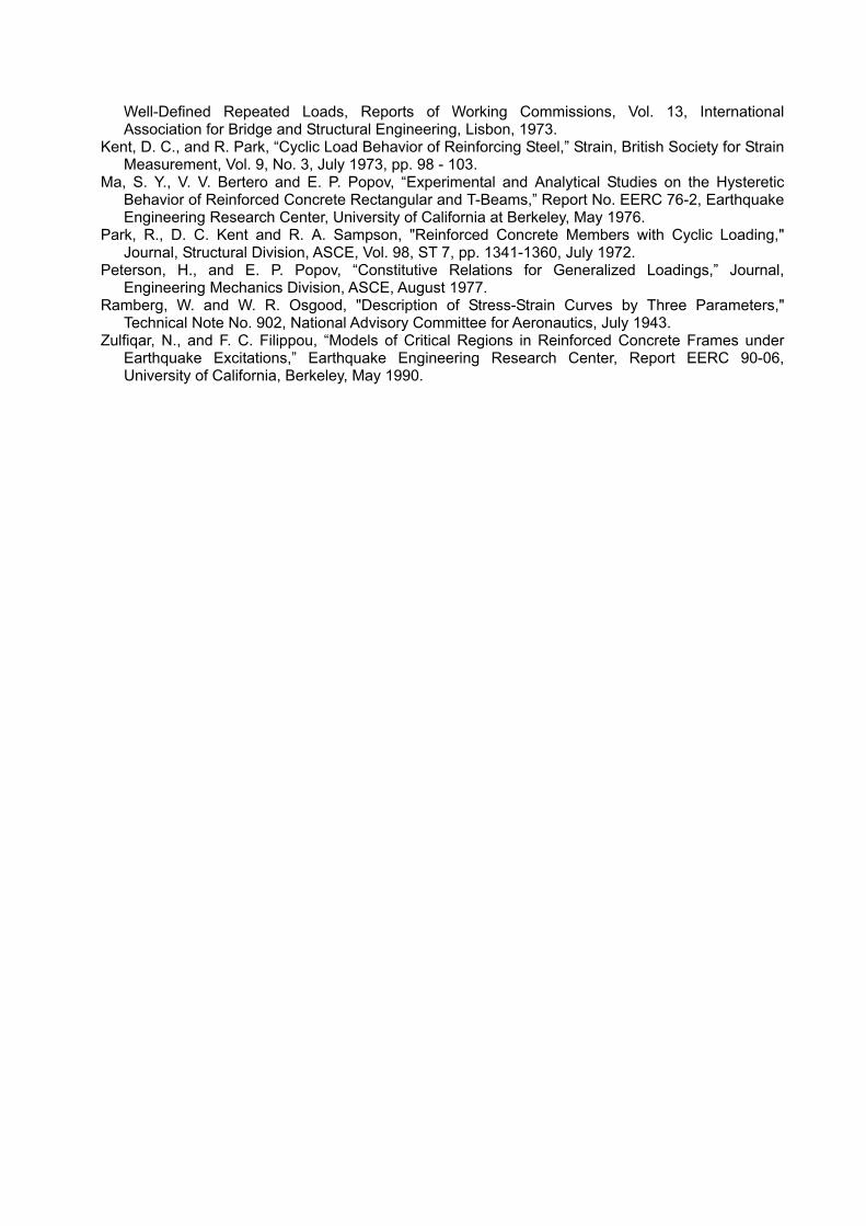
Well-Defined Repeated Loads, Reports of Working Commissions, Vol. 13, International Association for Bridge and Structural Engineering, Lisbon, 1973.

Kent, D. C., and R. Park, “Cyclic Load Behavior of Reinforcing Steel,” Strain, British Society for Strain Measurement, Vol. 9, No. 3, July 1973, pp. 98 - 103.

Ma, S. Y., V. V. Bertero and E. P. Popov, “Experimental and Analytical Studies on the Hysteretic Behavior of Reinforced Concrete Rectangular and T-Beams,” Report No. EERC 76-2, Earthquake Engineering Research Center, University of California at Berkeley, May 1976.

Park, R., D. C. Kent and R. A. Sampson, "Reinforced Concrete Members with Cyclic Loading," Journal, Structural Division, ASCE, Vol. 98, ST 7, pp. 1341-1360, July 1972.

Peterson, H., and E. P. Popov, “Constitutive Relations for Generalized Loadings,” Journal, Engineering Mechanics Division, ASCE, August 1977.

Ramberg, W. and W. R. Osgood, "Description of Stress-Strain Curves by Three Parameters," Technical Note No. 902, National Advisory Committee for Aeronautics, July 1943.

Zulfiqar, N., and F. C. Filippou, “Models of Critical Regions in Reinforced Concrete Frames under Earthquake Excitations,” Earthquake Engineering Research Center, Report EERC 90-06, University of California, Berkeley, May 1990.

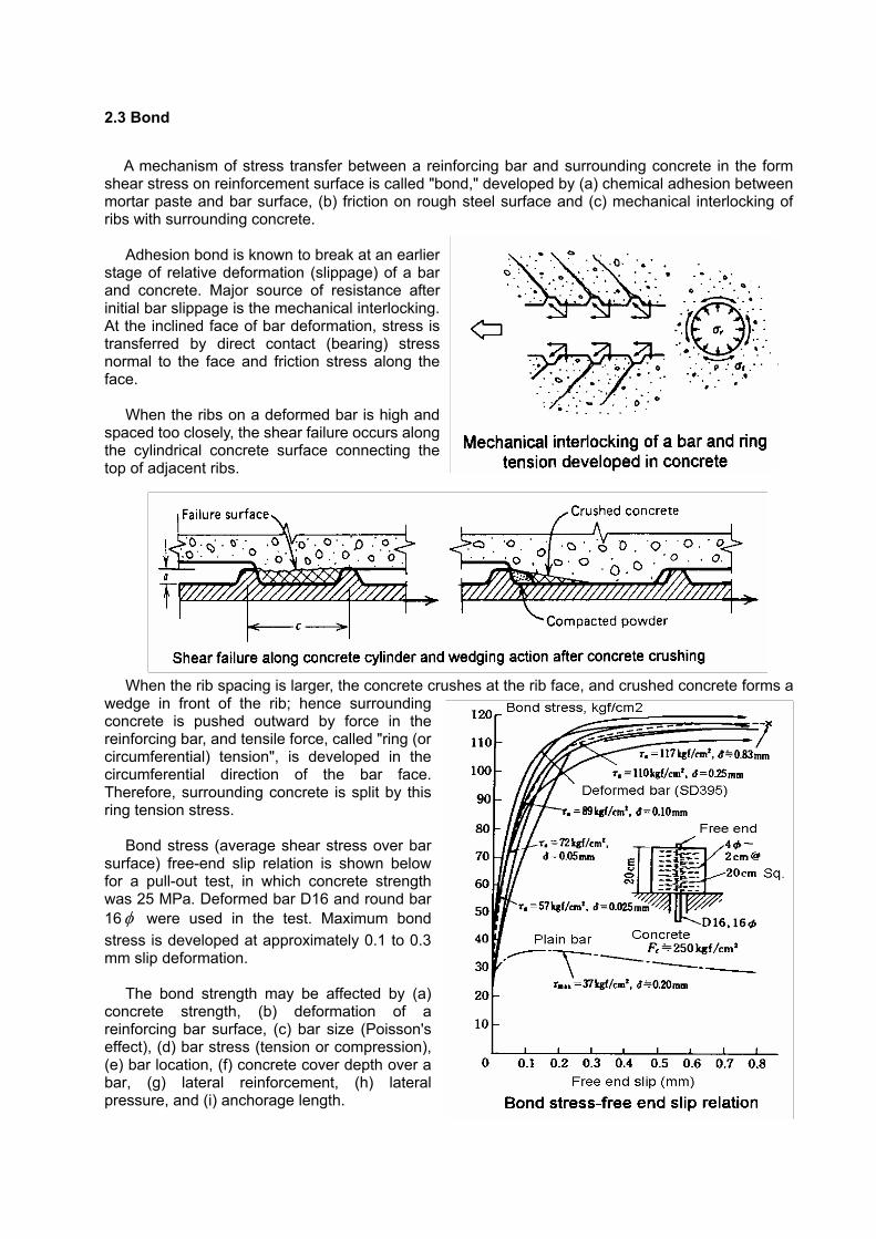
2.3 Bond

A mechanism of stress transfer between a reinforcing bar and surrounding concrete in the form shear stress on reinforcement surface is called "bond," developed by (a) chemical adhesion between mortar paste and bar surface, (b) friction on rough steel surface and (c) mechanical interlocking of ribs with surrounding concrete.

Adhesion bond is known to break at an earlier

stage of relative deformation (slippage) of a bar and concrete. Major source of resistance after initial bar slippage is the mechanical interlocking. At the inclined face of bar deformation, stress is transferred by direct contact (bearing) stress normal to the face and friction stress along the face.

When the ribs on a deformed bar is high and

spaced too closely, the shear failure occurs along the cylindrical concrete surface connecting the top of adjacent ribs.

When the rib spacing is larger, the concrete crushes at the rib face, and crushed concrete forms a wedge in front of the rib; hence surrounding concrete is pushed outward by force in the reinforcing bar, and tensile force, called "ring (or circumferential) tension", is developed in the circumferential direction of the bar face. Therefore, surrounding concrete is split by this ring tension stress.

Bond stress (average shear stress over bar

surface) free-end slip relation is shown below for a pull-out test, in which concrete strength was 25 MPa. Deformed bar D16 and round bar 16φ were used in the test. Maximum bond stress is developed at approximately 0.1 to 0.3 mm slip deformation.

The bond strength may be affected by (a)

concrete strength, (b) deformation of a reinforcing bar surface, (c) bar size (Poisson's effect), (d) bar stress (tension or compression), (e) bar location, (f) concrete cover depth over a bar, (g) lateral reinforcement, (h) lateral pressure, and (i) anchorage length.

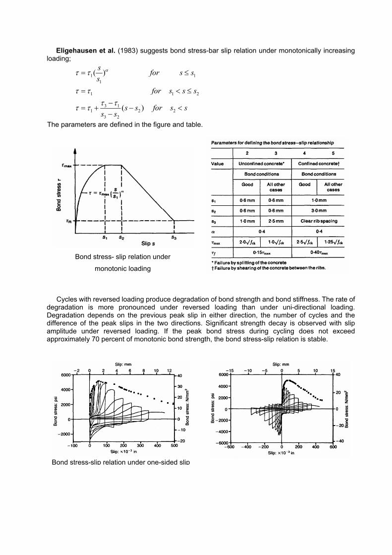
Eligehausen et al. (1983) suggests bond stress-bar slip relation under monotonically increasing loading;

1 11

1 1 2

3 11 2 2

3 2

( )

( )

s for s ss

for s s s

s s for s ss s

ατ τ

τ ττ ττ τ

= ≤

= < ≤−

= + − <−

The parameters are defined in the figure and table.

Cycles with reversed loading produce degradation of bond strength and bond stiffness. The rate of degradation is more pronounced under reversed loading than under uni-directional loading. Degradation depends on the previous peak slip in either direction, the number of cycles and the difference of the peak slips in the two directions. Significant strength decay is observed with slip amplitude under reversed loading. If the peak bond stress during cycling does not exceed approximately 70 percent of monotonic bond strength, the bond stress-slip relation is stable.

Bond stress-slip relation under one-sided slip

Bond stress- slip relation under

monotonic loading

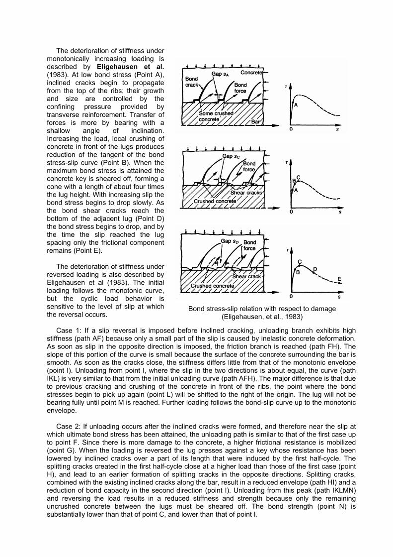
The deterioration of stiffness under monotonically increasing loading is described by Eligehausen et al. (1983). At low bond stress (Point A), inclined cracks begin to propagate from the top of the ribs; their growth and size are controlled by the confining pressure provided by transverse reinforcement. Transfer of forces is more by bearing with a shallow angle of inclination. Increasing the load, local crushing of concrete in front of the lugs produces reduction of the tangent of the bond stress-slip curve (Point B). When the maximum bond stress is attained the concrete key is sheared off, forming a cone with a length of about four times the lug height. With increasing slip the bond stress begins to drop slowly. As the bond shear cracks reach the bottom of the adjacent lug (Point D) the bond stress begins to drop, and by the time the slip reached the lug spacing only the frictional component remains (Point E).

The deterioration of stiffness under

reversed loading is also described by Eligehausen et al (1983). The initial loading follows the monotonic curve, but the cyclic load behavior is sensitive to the level of slip at which the reversal occurs.

Case 1: If a slip reversal is imposed before inclined cracking, unloading branch exhibits high

stiffness (path AF) because only a small part of the slip is caused by inelastic concrete deformation. As soon as slip in the opposite direction is imposed, the friction branch is reached (path FH). The slope of this portion of the curve is small because the surface of the concrete surrounding the bar is smooth. As soon as the cracks close, the stiffness differs little from that of the monotonic envelope (point I). Unloading from point I, where the slip in the two directions is about equal, the curve (path IKL) is very similar to that from the initial unloading curve (path AFH). The major difference is that due to previous cracking and crushing of the concrete in front of the ribs, the point where the bond stresses begin to pick up again (point L) will be shifted to the right of the origin. The lug will not be bearing fully until point M is reached. Further loading follows the bond-slip curve up to the monotonic envelope.

Case 2: If unloading occurs after the inclined cracks were formed, and therefore near the slip at

which ultimate bond stress has been attained, the unloading path is similar to that of the first case up to point F. Since there is more damage to the concrete, a higher frictional resistance is mobilized (point G). When the loading is reversed the lug presses against a key whose resistance has been lowered by inclined cracks over a part of its length that were induced by the first half-cycle. The splitting cracks created in the first half-cycle close at a higher load than those of the first case (point H), and lead to an earlier formation of splitting cracks in the opposite directions. Splitting cracks, combined with the existing inclined cracks along the bar, result in a reduced envelope (path HI) and a reduction of bond capacity in the second direction (point I). Unloading from this peak (path IKLMN) and reversing the load results in a reduced stiffness and strength because only the remaining uncrushed concrete between the lugs must be sheared off. The bond strength (point N) is substantially lower than that of point C, and lower than that of point I.

Bond stress-slip relation with respect to damage (Eligehausen, et al., 1983)

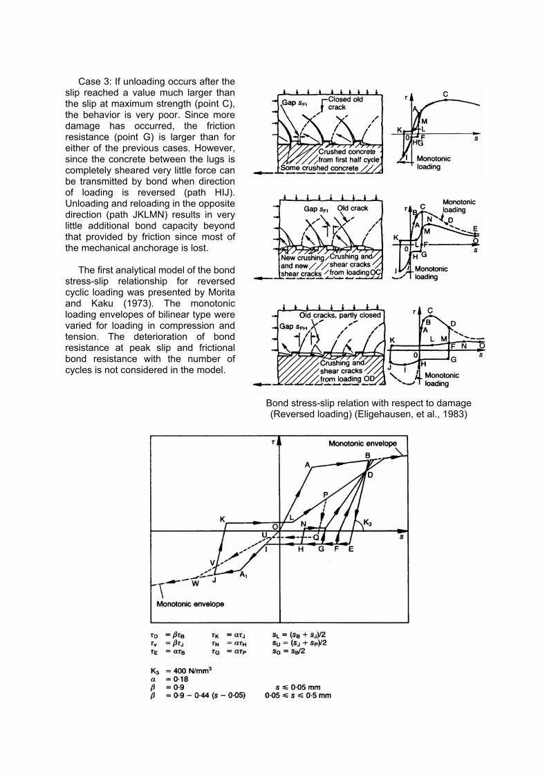
Case 3: If unloading occurs after the

slip reached a value much larger than the slip at maximum strength (point C), the behavior is very poor. Since more damage has occurred, the friction resistance (point G) is larger than for either of the previous cases. However, since the concrete between the lugs is completely sheared very little force can be transmitted by bond when direction of loading is reversed (path HIJ). Unloading and reloading in the opposite direction (path JKLMN) results in very little additional bond capacity beyond that provided by friction since most of the mechanical anchorage is lost.

The first analytical model of the bond

stress-slip relationship for reversed cyclic loading was presented by Morita and Kaku (1973). The monotonic loading envelopes of bilinear type were varied for loading in compression and tension. The deterioration of bond resistance at peak slip and frictional bond resistance with the number of cycles is not considered in the model.

Bond stress-slip relation with respect to damage (Reversed loading) (Eligehausen, et al., 1983)

Additional models for bond stress-bar slip hysteresis models can be found in Refs. Viwathanatepa, S. and et al. (1979), Hawkins et al. (1982) and Balaz (1989). References: Balazs, G. L., “Bond Softening under Reversed Load Cycles,” Stui e Ricerche - Corso Flli. Presenti,

Pollitecnico di Milano, No. 11, 1989, pp. 503 - 524. Eligehausen, R., V. V. Bertero, and E. Popov, “Local Bond Stress-slip Relationships of Deformed

Bars under Generalized Excitations,” Earthquake Engineering Research Center, Report No. EERC 83-23, University of California, Berkeley, October 1983.

Hawkins, H. M., et al., “Local Bond Strength of Concrete for Cyclic Reversed Loadings,” Bond in Concrete, P. Bartos (ed.), Applied Science Publishers Ltd., London, 1982, pp. 151 - 161.

Morita, S. and T. Kaku, “Local Bond Stress-slip Relationship under Repeated Loading,” Proceedings, IABSE Symposium on Resistance and Ultimate Deformability on Structures Acted on by Well Defined Repeated Loads, Lisbon, 1973, pp. 221 - 227.

Viwathanatepa, S. and et al., “Effect of Generalized loadings on Bond of Reinforcing Bars embedded in Confined Concrete Blocks,” Earthquake Engineering Research Center, Report No. EERC 79/22, University of California, Berkeley, August 1979.

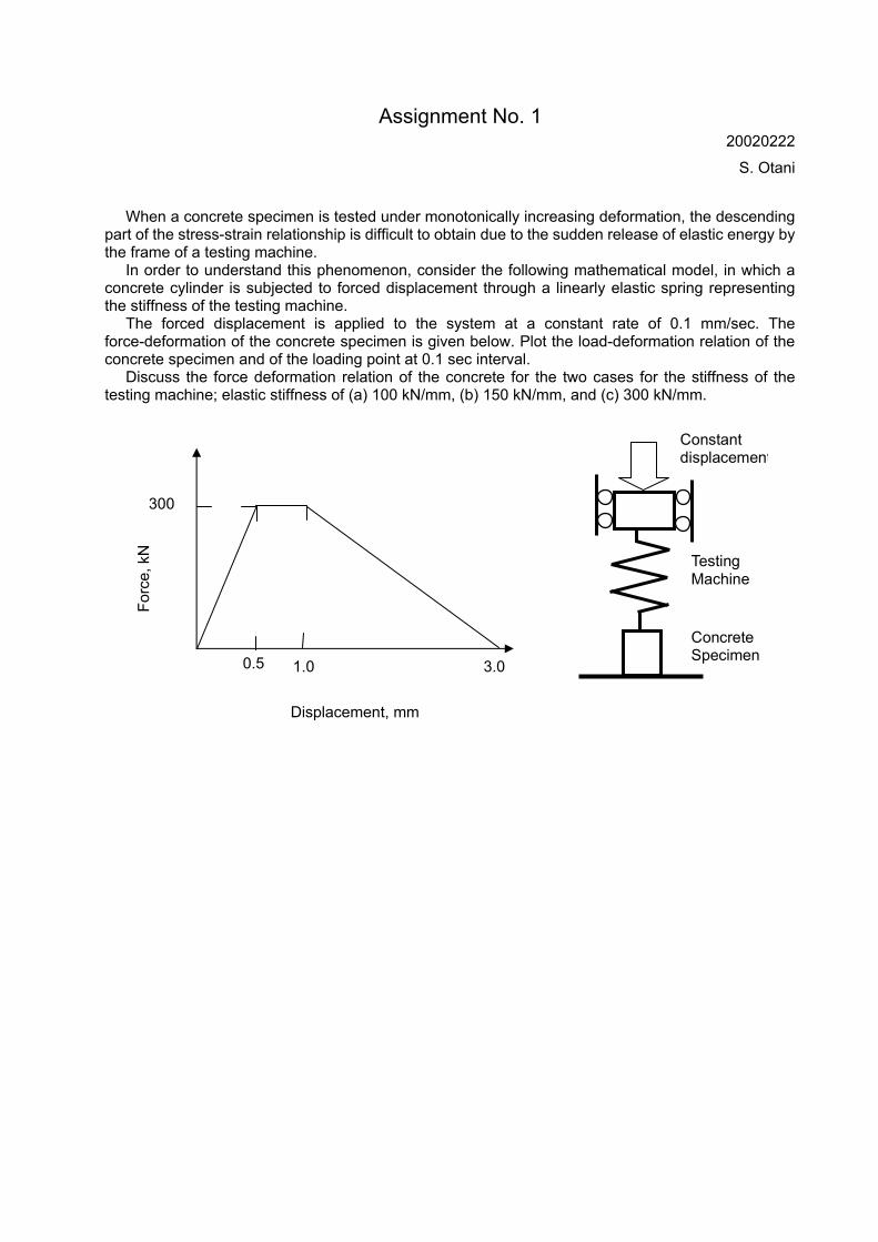
Assignment No. 1 20020222

S. Otani

When a concrete specimen is tested under monotonically increasing deformation, the descending

part of the stress-strain relationship is difficult to obtain due to the sudden release of elastic energy by the frame of a testing machine.

In order to understand this phenomenon, consider the following mathematical model, in which a concrete cylinder is subjected to forced displacement through a linearly elastic spring representing the stiffness of the testing machine.

The forced displacement is applied to the system at a constant rate of 0.1 mm/sec. The force-deformation of the concrete specimen is given below. Plot the load-deformation relation of the concrete specimen and of the loading point at 0.1 sec interval.

Discuss the force deformation relation of the concrete for the two cases for the stiffness of the testing machine; elastic stiffness of (a) 100 kN/mm, (b) 150 kN/mm, and (c) 300 kN/mm.

0.5 1.0 3.0

Displacement, mm

300

Forc

e, k

N

Testing Machine

Concrete Specimen

Constant displacement

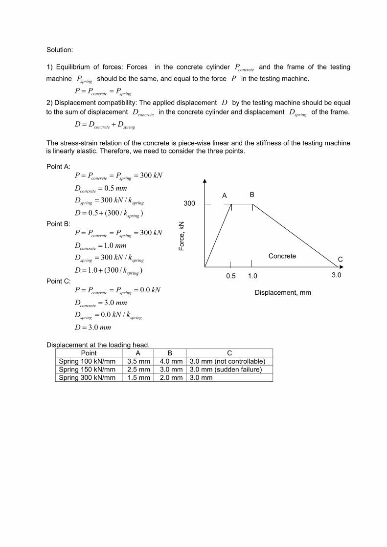
Solution: 1) Equilibrium of forces: Forces in the concrete cylinder concreteP and the frame of the testing

machine springP should be the same, and equal to the force P in the testing machine.

concrete springP P P= =

2) Displacement compatibility: The applied displacement D by the testing machine should be equal to the sum of displacement concreteD in the concrete cylinder and displacement springD of the frame.

concrete springD D D= + The stress-strain relation of the concrete is piece-wise linear and the stiffness of the testing machine is linearly elastic. Therefore, we need to consider the three points. Point A:

300

0.5300 /

0.5 (300 / )

concrete spring

concrete

spring spring

spring

P P P kND mmD kN kD k

= = =

==

= +

Point B:

300

1.0300 /

1.0 (300 / )

concrete spring

concrete

spring spring

spring

P P P kND mmD kN kD k

= = =

==

= +

Point C:

0.0

3.00.0 /

3.0

concrete spring

concrete

spring spring

P P P kND mmD kN kD mm

= = =

==

=

Displacement at the loading head.

Point A B C Spring 100 kN/mm 3.5 mm 4.0 mm 3.0 mm (not controllable) Spring 150 kN/mm 2.5 mm 3.0 mm 3.0 mm (sudden failure) Spring 300 kN/mm 1.5 mm 2.0 mm 3.0 mm

0.5 1.0 3.0

A B

CConcrete

Displacement, mm

300

Forc

e, k

N

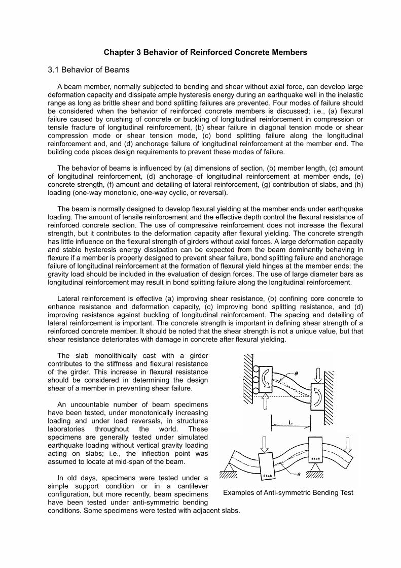
Chapter 3 Behavior of Reinforced Concrete Members 3.1 Behavior of Beams

A beam member, normally subjected to bending and shear without axial force, can develop large deformation capacity and dissipate ample hysteresis energy during an earthquake well in the inelastic range as long as brittle shear and bond splitting failures are prevented. Four modes of failure should be considered when the behavior of reinforced concrete members is discussed; i.e., (a) flexural failure caused by crushing of concrete or buckling of longitudinal reinforcement in compression or tensile fracture of longitudinal reinforcement, (b) shear failure in diagonal tension mode or shear compression mode or shear tension mode, (c) bond splitting failure along the longitudinal reinforcement and, and (d) anchorage failure of longitudinal reinforcement at the member end. The building code places design requirements to prevent these modes of failure.

The behavior of beams is influenced by (a) dimensions of section, (b) member length, (c) amount

of longitudinal reinforcement, (d) anchorage of longitudinal reinforcement at member ends, (e) concrete strength, (f) amount and detailing of lateral reinforcement, (g) contribution of slabs, and (h) loading (one-way monotonic, one-way cyclic, or reversal).

The beam is normally designed to develop flexural yielding at the member ends under earthquake

loading. The amount of tensile reinforcement and the effective depth control the flexural resistance of reinforced concrete section. The use of compressive reinforcement does not increase the flexural strength, but it contributes to the deformation capacity after flexural yielding. The concrete strength has little influence on the flexural strength of girders without axial forces. A large deformation capacity and stable hysteresis energy dissipation can be expected from the beam dominantly behaving in flexure if a member is properly designed to prevent shear failure, bond splitting failure and anchorage failure of longitudinal reinforcement at the formation of flexural yield hinges at the member ends; the gravity load should be included in the evaluation of design forces. The use of large diameter bars as longitudinal reinforcement may result in bond splitting failure along the longitudinal reinforcement.

Lateral reinforcement is effective (a) improving shear resistance, (b) confining core concrete to

enhance resistance and deformation capacity, (c) improving bond splitting resistance, and (d) improving resistance against buckling of longitudinal reinforcement. The spacing and detailing of lateral reinforcement is important. The concrete strength is important in defining shear strength of a reinforced concrete member. It should be noted that the shear strength is not a unique value, but that shear resistance deteriorates with damage in concrete after flexural yielding.

The slab monolithically cast with a girder

contributes to the stiffness and flexural resistance of the girder. This increase in flexural resistance should be considered in determining the design shear of a member in preventing shear failure.

An uncountable number of beam specimens

have been tested, under monotonically increasing loading and under load reversals, in structures laboratories throughout the world. These specimens are generally tested under simulated earthquake loading without vertical gravity loading acting on slabs; i.e., the inflection point was assumed to locate at mid-span of the beam.

In old days, specimens were tested under a

simple support condition or in a cantilever configuration, but more recently, beam specimens have been tested under anti-symmetric bending conditions. Some specimens were tested with adjacent slabs.

Examples of Anti-symmetric Bending Test

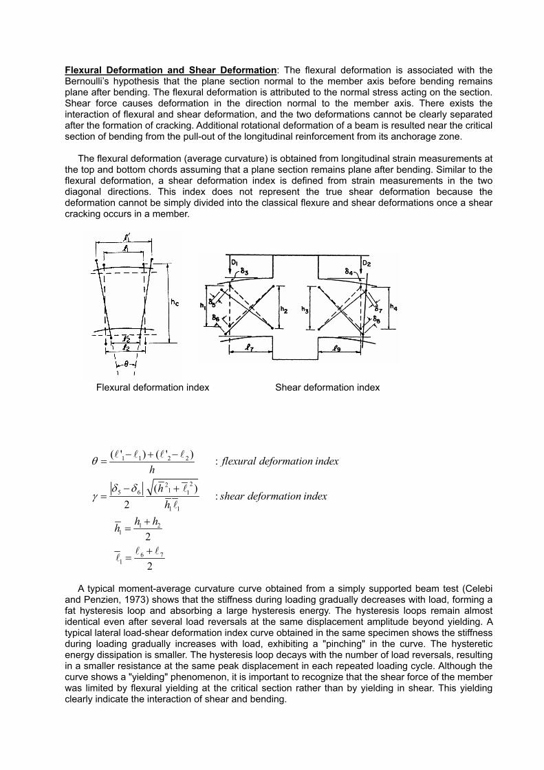
Flexural Deformation and Shear Deformation: The flexural deformation is associated with the Bernoulli’s hypothesis that the plane section normal to the member axis before bending remains plane after bending. The flexural deformation is attributed to the normal stress acting on the section. Shear force causes deformation in the direction normal to the member axis. There exists the interaction of flexural and shear deformation, and the two deformations cannot be clearly separated after the formation of cracking. Additional rotational deformation of a beam is resulted near the critical section of bending from the pull-out of the longitudinal reinforcement from its anchorage zone.

The flexural deformation (average curvature) is obtained from longitudinal strain measurements at the top and bottom chords assuming that a plane section remains plane after bending. Similar to the flexural deformation, a shear deformation index is defined from strain measurements in the two diagonal directions. This index does not represent the true shear deformation because the deformation cannot be simply divided into the classical flexure and shear deformations once a shear cracking occurs in a member.

1 1 2 2

2215 6 1

1 1

1 21

6 71

( ' ) ( ' ) :

( ):

2

2

2

flexural deformation indexh

hshear deformation index

hh hh

θ

δ δγ

− + −=

− +=

+=

+=

A typical moment-average curvature curve obtained from a simply supported beam test (Celebi

and Penzien, 1973) shows that the stiffness during loading gradually decreases with load, forming a fat hysteresis loop and absorbing a large hysteresis energy. The hysteresis loops remain almost identical even after several load reversals at the same displacement amplitude beyond yielding. A typical lateral load-shear deformation index curve obtained in the same specimen shows the stiffness during loading gradually increases with load, exhibiting a "pinching" in the curve. The hysteretic energy dissipation is smaller. The hysteresis loop decays with the number of load reversals, resulting in a smaller resistance at the same peak displacement in each repeated loading cycle. Although the curve shows a "yielding" phenomenon, it is important to recognize that the shear force of the member was limited by flexural yielding at the critical section rather than by yielding in shear. This yielding clearly indicate the interaction of shear and bending.

Flexural deformation index Shear deformation index

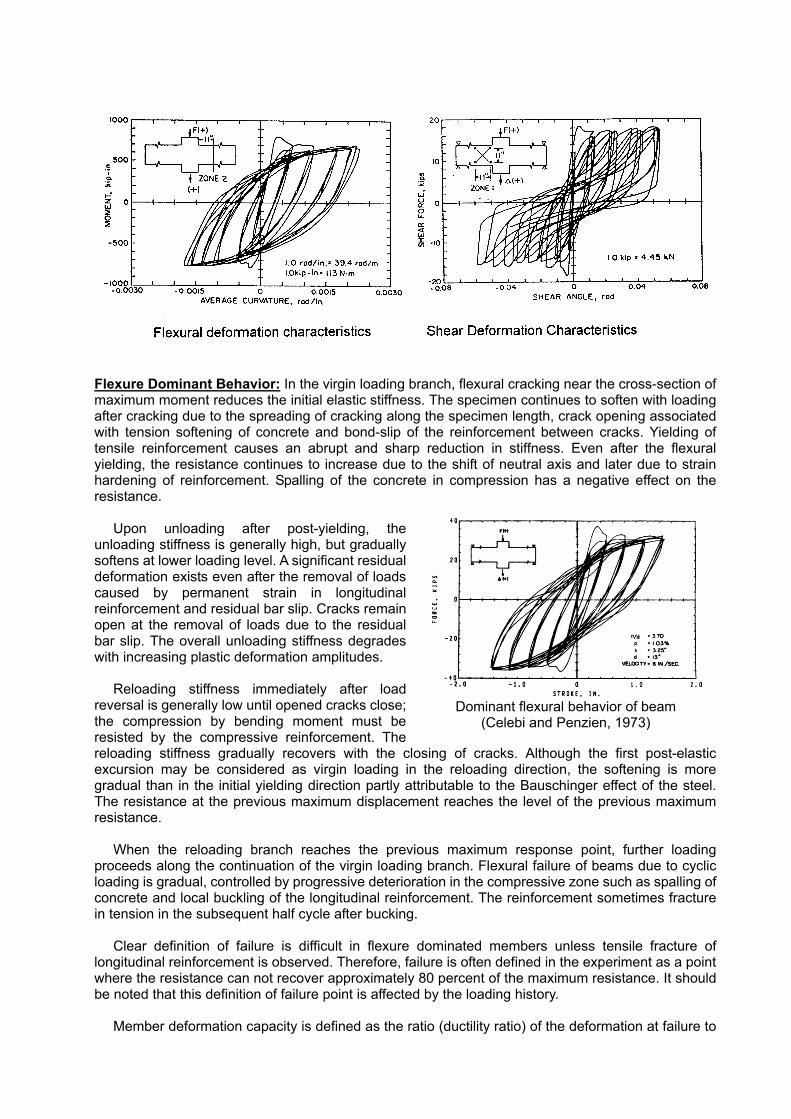
Flexure Dominant Behavior: In the virgin loading branch, flexural cracking near the cross-section of maximum moment reduces the initial elastic stiffness. The specimen continues to soften with loading after cracking due to the spreading of cracking along the specimen length, crack opening associated with tension softening of concrete and bond-slip of the reinforcement between cracks. Yielding of tensile reinforcement causes an abrupt and sharp reduction in stiffness. Even after the flexural yielding, the resistance continues to increase due to the shift of neutral axis and later due to strain hardening of reinforcement. Spalling of the concrete in compression has a negative effect on the resistance.

Upon unloading after post-yielding, the unloading stiffness is generally high, but gradually softens at lower loading level. A significant residual deformation exists even after the removal of loads caused by permanent strain in longitudinal reinforcement and residual bar slip. Cracks remain open at the removal of loads due to the residual bar slip. The overall unloading stiffness degrades with increasing plastic deformation amplitudes.

Reloading stiffness immediately after load

reversal is generally low until opened cracks close; the compression by bending moment must be resisted by the compressive reinforcement. The reloading stiffness gradually recovers with the closing of cracks. Although the first post-elastic excursion may be considered as virgin loading in the reloading direction, the softening is more gradual than in the initial yielding direction partly attributable to the Bauschinger effect of the steel. The resistance at the previous maximum displacement reaches the level of the previous maximum resistance.

When the reloading branch reaches the previous maximum response point, further loading

proceeds along the continuation of the virgin loading branch. Flexural failure of beams due to cyclic loading is gradual, controlled by progressive deterioration in the compressive zone such as spalling of concrete and local buckling of the longitudinal reinforcement. The reinforcement sometimes fracture in tension in the subsequent half cycle after bucking.

Clear definition of failure is difficult in flexure dominated members unless tensile fracture of

longitudinal reinforcement is observed. Therefore, failure is often defined in the experiment as a point where the resistance can not recover approximately 80 percent of the maximum resistance. It should be noted that this definition of failure point is affected by the loading history.

Member deformation capacity is defined as the ratio (ductility ratio) of the deformation at failure to

Dominant flexural behavior of beam (Celebi and Penzien, 1973)

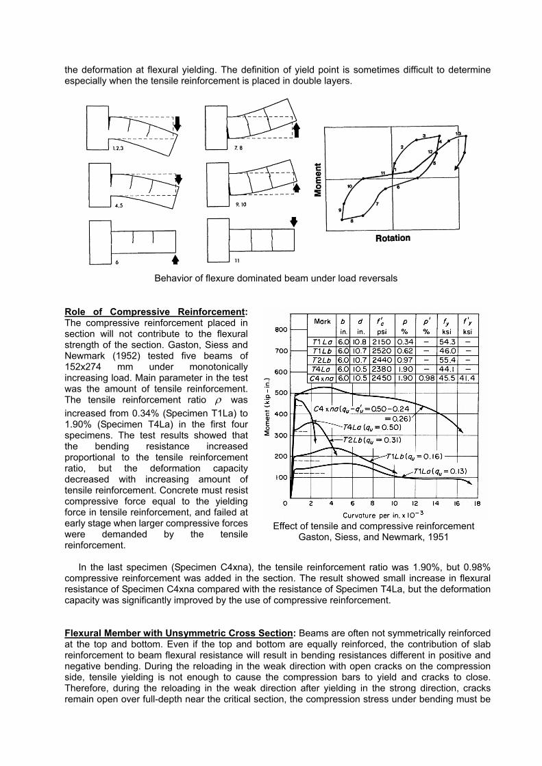
the deformation at flexural yielding. The definition of yield point is sometimes difficult to determine especially when the tensile reinforcement is placed in double layers.

Role of Compressive Reinforcement: The compressive reinforcement placed in section will not contribute to the flexural strength of the section. Gaston, Siess and Newmark (1952) tested five beams of 152x274 mm under monotonically increasing load. Main parameter in the test was the amount of tensile reinforcement. The tensile reinforcement ratio ρ was increased from 0.34% (Specimen T1La) to 1.90% (Specimen T4La) in the first four specimens. The test results showed that the bending resistance increased proportional to the tensile reinforcement ratio, but the deformation capacity decreased with increasing amount of tensile reinforcement. Concrete must resist compressive force equal to the yielding force in tensile reinforcement, and failed at early stage when larger compressive forces were demanded by the tensile reinforcement.

In the last specimen (Specimen C4xna), the tensile reinforcement ratio was 1.90%, but 0.98% compressive reinforcement was added in the section. The result showed small increase in flexural resistance of Specimen C4xna compared with the resistance of Specimen T4La, but the deformation capacity was significantly improved by the use of compressive reinforcement. Flexural Member with Unsymmetric Cross Section: Beams are often not symmetrically reinforced at the top and bottom. Even if the top and bottom are equally reinforced, the contribution of slab reinforcement to beam flexural resistance will result in bending resistances different in positive and negative bending. During the reloading in the weak direction with open cracks on the compression side, tensile yielding is not enough to cause the compression bars to yield and cracks to close. Therefore, during the reloading in the weak direction after yielding in the strong direction, cracks remain open over full-depth near the critical section, the compression stress under bending must be

Behavior of flexure dominated beam under load reversals

Effect of tensile and compressive reinforcement Gaston, Siess, and Newmark, 1951

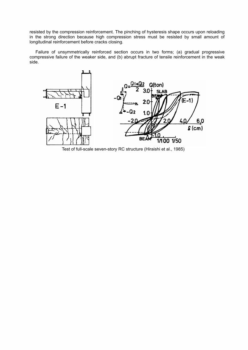
resisted by the compression reinforcement. The pinching of hysteresis shape occurs upon reloading in the strong direction because high compression stress must be resisted by small amount of longitudinal reinforcement before cracks closing.

Failure of unsymmetrically reinforced section occurs in two forms; (a) gradual progressive compressive failure of the weaker side, and (b) abrupt fracture of tensile reinforcement in the weak side.

Test of full-scale seven-story RC structure (Hiraishi et al., 1985)

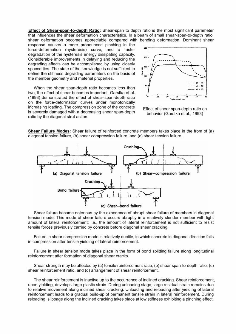
Effect of Shear-span-to-depth Ratio: Shear-span to depth ratio is the most significant parameter that influences the shear deformation characteristics. In a beam of small shear-span-to-depth ratio, shear deformation becomes appreciable compared with bending deformation. Dominant shear response causes a more pronounced pinching in the force-deformation (hysteresis) curve, and a faster degradation of the hysteresis energy dissipating capacity. Considerable improvements in delaying and reducing the degrading effects can be accomplished by using closely spaced ties. The state of the knowledge is not sufficient to define the stiffness degrading parameters on the basis of the member geometry and material properties.

When the shear span-depth ratio becomes less than two, the effect of shear becomes important. Garstka et al. (1993) demonstrated the effect of shear-span-depth ratio on the force-deformation curves under monotonically increasing loading. The compression zone of the concrete is severely damaged with a decreasing shear span-depth ratio by the diagonal strut action.

Shear Failure Modes: Shear failure of reinforced concrete members takes place in the from of (a) diagonal tension failure, (b) shear compression failure, and (c) shear tension failure.

Shear failure became notorious by the experience of abrupt shear failure of members in diagonal tension mode. This mode of shear failure occurs abruptly in a relatively slender member with light amount of lateral reinforcement; i.e., the amount of lateral reinforcement is not sufficient to resist tensile forces previously carried by concrete before diagonal shear cracking.

Failure in shear compression mode is relatively ductile, in which concrete in diagonal direction fails

in compression after tensile yielding of lateral reinforcement. Failure in shear tension mode takes place in the form of bond splitting failure along longitudinal

reinforcement after formation of diagonal shear cracks. Shear strength may be affected by (a) tensile reinforcement ratio, (b) shear span-to-depth ratio, (c)

shear reinforcement ratio, and (d) arrangement of shear reinforcement. The shear reinforcement is inactive up to the occurrence of inclined cracking. Shear reinforcement,

upon yielding, develops large plastic strain. During unloading stage, large residual strain remains due to relative movement along inclined shear cracking. Unloading and reloading after yielding of lateral reinforcement leads to a gradual build-up of permanent tensile strain in lateral reinforcement. During reloading, slippage along the inclined cracking takes place at low stiffness exhibiting a pinching effect.

Effect of shear span-depth ratio on

behavior (Garstka et al., 1993)

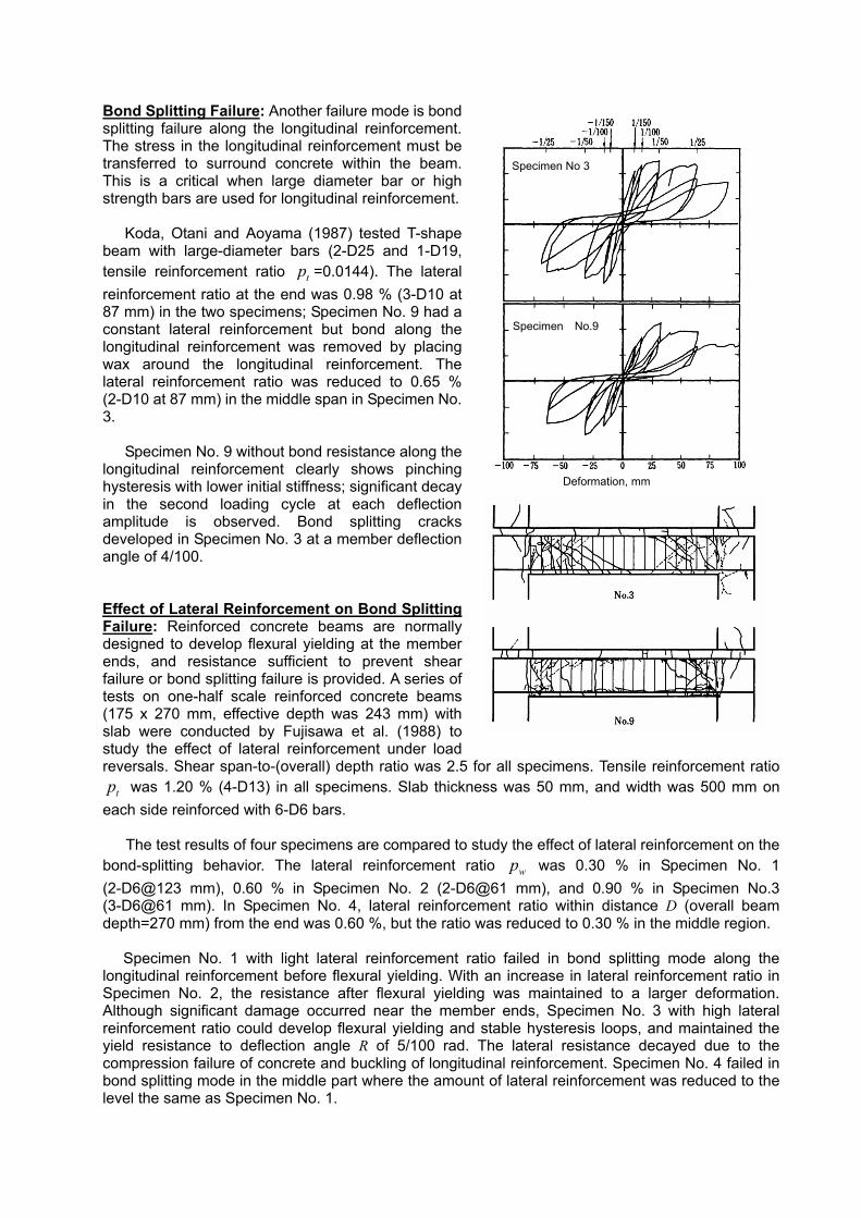
Bond Splitting Failure: Another failure mode is bond splitting failure along the longitudinal reinforcement. The stress in the longitudinal reinforcement must be transferred to surround concrete within the beam. This is a critical when large diameter bar or high strength bars are used for longitudinal reinforcement.

Koda, Otani and Aoyama (1987) tested T-shape beam with large-diameter bars (2-D25 and 1-D19, tensile reinforcement ratio tp =0.0144). The lateral reinforcement ratio at the end was 0.98 % (3-D10 at 87 mm) in the two specimens; Specimen No. 9 had a constant lateral reinforcement but bond along the longitudinal reinforcement was removed by placing wax around the longitudinal reinforcement. The lateral reinforcement ratio was reduced to 0.65 % (2-D10 at 87 mm) in the middle span in Specimen No. 3.

Specimen No. 9 without bond resistance along the

longitudinal reinforcement clearly shows pinching hysteresis with lower initial stiffness; significant decay in the second loading cycle at each deflection amplitude is observed. Bond splitting cracks developed in Specimen No. 3 at a member deflection angle of 4/100. Effect of Lateral Reinforcement on Bond Splitting Failure: Reinforced concrete beams are normally designed to develop flexural yielding at the member ends, and resistance sufficient to prevent shear failure or bond splitting failure is provided. A series of tests on one-half scale reinforced concrete beams (175 x 270 mm, effective depth was 243 mm) with slab were conducted by Fujisawa et al. (1988) to study the effect of lateral reinforcement under load reversals. Shear span-to-(overall) depth ratio was 2.5 for all specimens. Tensile reinforcement ratio

tp was 1.20 % (4-D13) in all specimens. Slab thickness was 50 mm, and width was 500 mm on each side reinforced with 6-D6 bars.

The test results of four specimens are compared to study the effect of lateral reinforcement on the bond-splitting behavior. The lateral reinforcement ratio wp was 0.30 % in Specimen No. 1 (2-D6@123 mm), 0.60 % in Specimen No. 2 (2-D6@61 mm), and 0.90 % in Specimen No.3 (3-D6@61 mm). In Specimen No. 4, lateral reinforcement ratio within distance D (overall beam depth=270 mm) from the end was 0.60 %, but the ratio was reduced to 0.30 % in the middle region.

Specimen No. 1 with light lateral reinforcement ratio failed in bond splitting mode along the

longitudinal reinforcement before flexural yielding. With an increase in lateral reinforcement ratio in Specimen No. 2, the resistance after flexural yielding was maintained to a larger deformation. Although significant damage occurred near the member ends, Specimen No. 3 with high lateral reinforcement ratio could develop flexural yielding and stable hysteresis loops, and maintained the yield resistance to deflection angle R of 5/100 rad. The lateral resistance decayed due to the compression failure of concrete and buckling of longitudinal reinforcement. Specimen No. 4 failed in bond splitting mode in the middle part where the amount of lateral reinforcement was reduced to the level the same as Specimen No. 1.

試験体 Specimen No 3

Specimen No.9

Deformation, mm

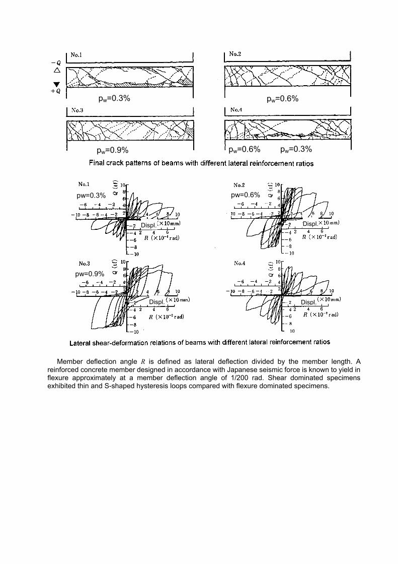
pw=0.3% pw=0.6%

pw=0.9% pw=0.6% pw=0.3%

Displ.

Displ.

Displ.

Displ.

pw=0.3% pw=0.6%

pw=0.9%

Member deflection angle R is defined as lateral deflection divided by the member length. A reinforced concrete member designed in accordance with Japanese seismic force is known to yield in flexure approximately at a member deflection angle of 1/200 rad. Shear dominated specimens exhibited thin and S-shaped hysteresis loops compared with flexure dominated specimens.

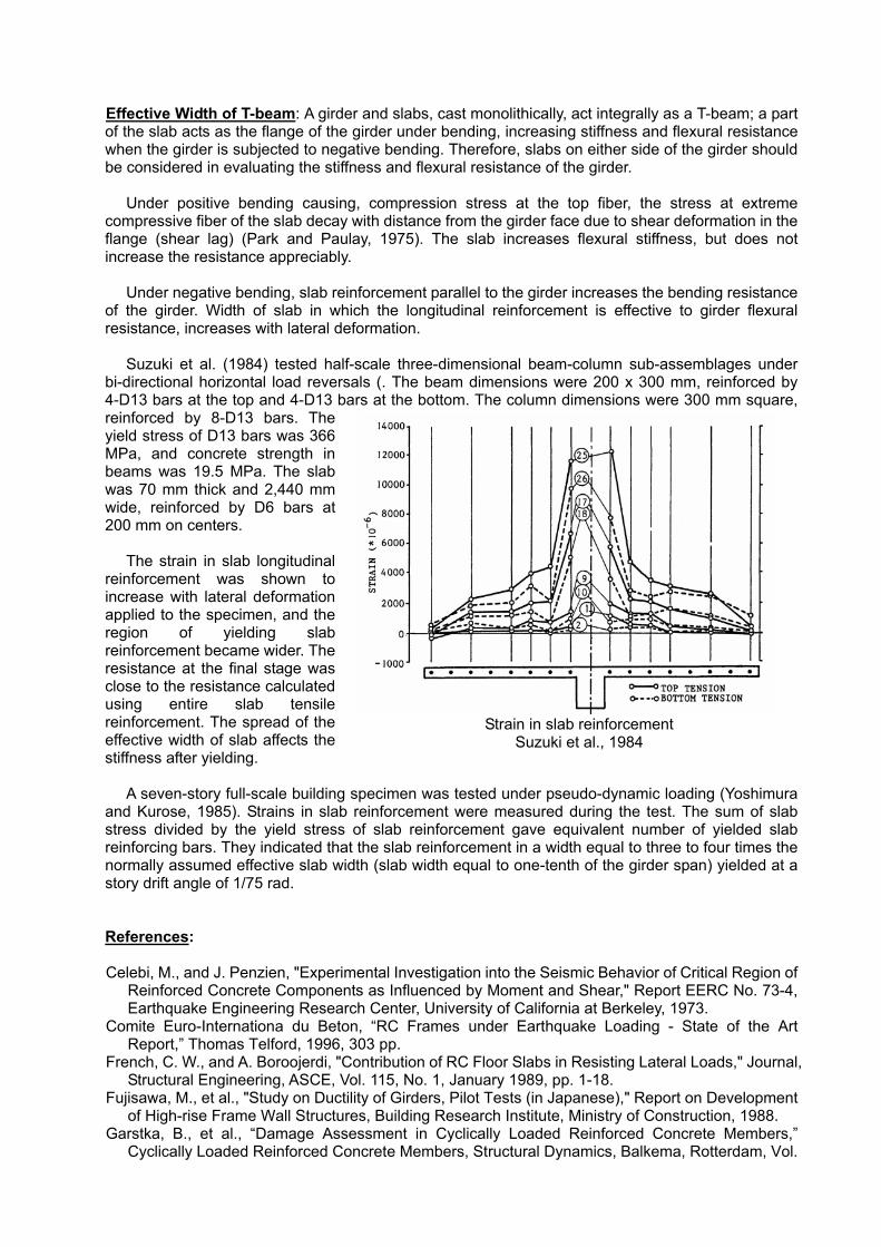
Effective Width of T-beam: A girder and slabs, cast monolithically, act integrally as a T-beam; a part of the slab acts as the flange of the girder under bending, increasing stiffness and flexural resistance when the girder is subjected to negative bending. Therefore, slabs on either side of the girder should be considered in evaluating the stiffness and flexural resistance of the girder.

Under positive bending causing, compression stress at the top fiber, the stress at extreme compressive fiber of the slab decay with distance from the girder face due to shear deformation in the flange (shear lag) (Park and Paulay, 1975). The slab increases flexural stiffness, but does not increase the resistance appreciably.

Under negative bending, slab reinforcement parallel to the girder increases the bending resistance

of the girder. Width of slab in which the longitudinal reinforcement is effective to girder flexural resistance, increases with lateral deformation.

Suzuki et al. (1984) tested half-scale three-dimensional beam-column sub-assemblages under

bi-directional horizontal load reversals (. The beam dimensions were 200 x 300 mm, reinforced by 4-D13 bars at the top and 4-D13 bars at the bottom. The column dimensions were 300 mm square, reinforced by 8-D13 bars. The yield stress of D13 bars was 366 MPa, and concrete strength in beams was 19.5 MPa. The slab was 70 mm thick and 2,440 mm wide, reinforced by D6 bars at 200 mm on centers.

The strain in slab longitudinal

reinforcement was shown to increase with lateral deformation applied to the specimen, and the region of yielding slab reinforcement became wider. The resistance at the final stage was close to the resistance calculated using entire slab tensile reinforcement. The spread of the effective width of slab affects the stiffness after yielding.

A seven-story full-scale building specimen was tested under pseudo-dynamic loading (Yoshimura

and Kurose, 1985). Strains in slab reinforcement were measured during the test. The sum of slab stress divided by the yield stress of slab reinforcement gave equivalent number of yielded slab reinforcing bars. They indicated that the slab reinforcement in a width equal to three to four times the normally assumed effective slab width (slab width equal to one-tenth of the girder span) yielded at a story drift angle of 1/75 rad.

References: Celebi, M., and J. Penzien, "Experimental Investigation into the Seismic Behavior of Critical Region of

Reinforced Concrete Components as Influenced by Moment and Shear," Report EERC No. 73-4, Earthquake Engineering Research Center, University of California at Berkeley, 1973.

Comite Euro-Internationa du Beton, “RC Frames under Earthquake Loading - State of the Art Report,” Thomas Telford, 1996, 303 pp.

French, C. W., and A. Boroojerdi, "Contribution of RC Floor Slabs in Resisting Lateral Loads," Journal, Structural Engineering, ASCE, Vol. 115, No. 1, January 1989, pp. 1-18.

Fujisawa, M., et al., "Study on Ductility of Girders, Pilot Tests (in Japanese)," Report on Development of High-rise Frame Wall Structures, Building Research Institute, Ministry of Construction, 1988.

Garstka, B., et al., “Damage Assessment in Cyclically Loaded Reinforced Concrete Members,” Cyclically Loaded Reinforced Concrete Members, Structural Dynamics, Balkema, Rotterdam, Vol.

Strain in slab reinforcement Suzuki et al., 1984

1, 1993, pp. 121 - 128. Hiraishi, H., S. Nakata, Y. Kitagawa and T. Kaminosono, “Static Tests on Shear Walls and

Beam-column Assemblies and Study on Correlation between Shaking Table Tests and Psuedo-dynamic Tests,” ACI SP-84, Earthquake Effects n Reinforced Concrete Structures, - U.S.-Japan Research, American Concrete Institute, 1985, pp. 11 - 48.

Koda, S., S. Otani and H. Aoyama, “Reinforcement Details of T-shape beams and Ductility (in Japanese),” Transactions, Architectural Institute of Japan Annual Convention, October 1987, pp. 209 - 210.

Ma, S. M., V. V. Bertero and E. P. Popov, "Experimental and Analytical Studies of the Hysteretic Behavior of Reinforced Concrete Members under Bidirectional Reversed Lateral Loading," Report No. EERC 76-2, University of California at Berkeley, 1976.

Park, R. and T. Paulay, Reinforced Concrete Structures, John Wiley & Sons, Inc., pp. 99-100, 1975. Suzuki, N., S. Otani and H. Aoyama, "Three-dimensional Beam-column Sub-assemblages under

Bi-directional Earthquake Loading," Proceedings, Eighth World Conference on Earthquake Engineering, Vol. VI, San Francisco, July 1984, pp. 453-460.

Yoshimura, M., and Y. Kurose, "Inelastic Behavior of the Building," ACI SP-84, Earthquake Effects on Reinforced Concrete Structure, US-Japan Research, American Concrete Institute, Detroit, 1985, pp. 163-202.

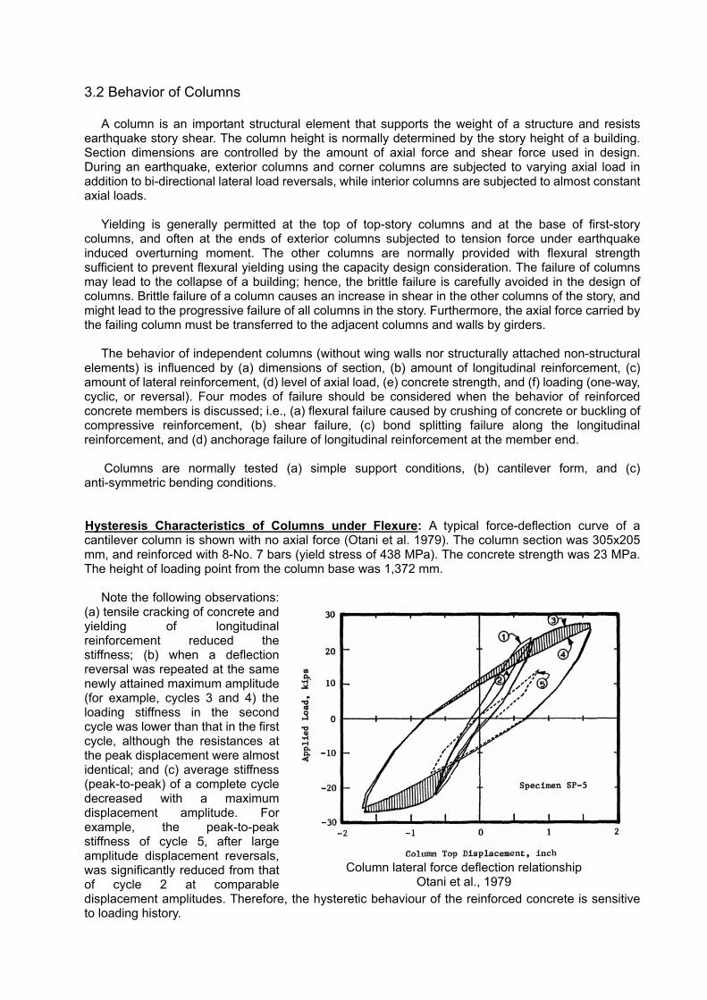
3.2 Behavior of Columns

A column is an important structural element that supports the weight of a structure and resists earthquake story shear. The column height is normally determined by the story height of a building. Section dimensions are controlled by the amount of axial force and shear force used in design. During an earthquake, exterior columns and corner columns are subjected to varying axial load in addition to bi-directional lateral load reversals, while interior columns are subjected to almost constant axial loads.

Yielding is generally permitted at the top of top-story columns and at the base of first-story

columns, and often at the ends of exterior columns subjected to tension force under earthquake induced overturning moment. The other columns are normally provided with flexural strength sufficient to prevent flexural yielding using the capacity design consideration. The failure of columns may lead to the collapse of a building; hence, the brittle failure is carefully avoided in the design of columns. Brittle failure of a column causes an increase in shear in the other columns of the story, and might lead to the progressive failure of all columns in the story. Furthermore, the axial force carried by the failing column must be transferred to the adjacent columns and walls by girders.

The behavior of independent columns (without wing walls nor structurally attached non-structural

elements) is influenced by (a) dimensions of section, (b) amount of longitudinal reinforcement, (c) amount of lateral reinforcement, (d) level of axial load, (e) concrete strength, and (f) loading (one-way, cyclic, or reversal). Four modes of failure should be considered when the behavior of reinforced concrete members is discussed; i.e., (a) flexural failure caused by crushing of concrete or buckling of compressive reinforcement, (b) shear failure, (c) bond splitting failure along the longitudinal reinforcement, and (d) anchorage failure of longitudinal reinforcement at the member end.

Columns are normally tested (a) simple support conditions, (b) cantilever form, and (c) anti-symmetric bending conditions. Hysteresis Characteristics of Columns under Flexure: A typical force-deflection curve of a cantilever column is shown with no axial force (Otani et al. 1979). The column section was 305x205 mm, and reinforced with 8-No. 7 bars (yield stress of 438 MPa). The concrete strength was 23 MPa. The height of loading point from the column base was 1,372 mm.

Note the following observations:

(a) tensile cracking of concrete and yielding of longitudinal reinforcement reduced the stiffness; (b) when a deflection reversal was repeated at the same newly attained maximum amplitude (for example, cycles 3 and 4) the loading stiffness in the second cycle was lower than that in the first cycle, although the resistances at the peak displacement were almost identical; and (c) average stiffness (peak-to-peak) of a complete cycle decreased with a maximum displacement amplitude. For example, the peak-to-peak stiffness of cycle 5, after large amplitude displacement reversals, was significantly reduced from that of cycle 2 at comparable displacement amplitudes. Therefore, the hysteretic behaviour of the reinforced concrete is sensitive to loading history.

Column lateral force deflection relationship Otani et al., 1979

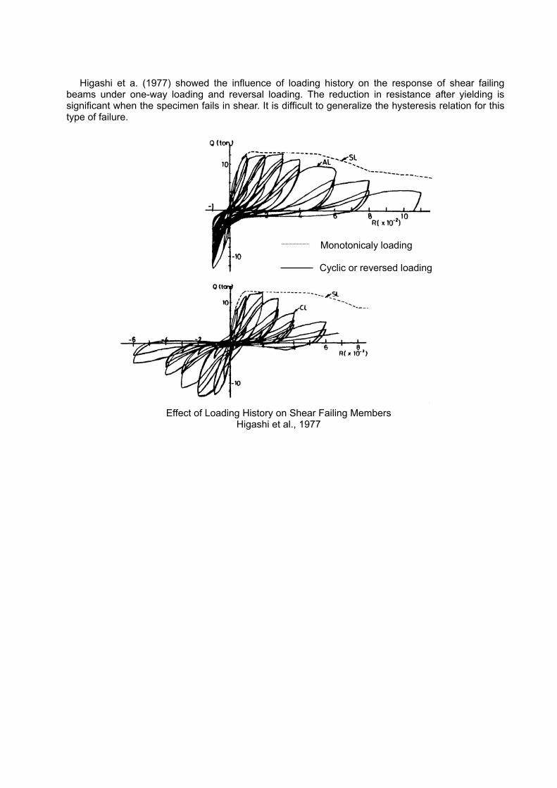
Higashi et a. (1977) showed the influence of loading history on the response of shear failing

beams under one-way loading and reversal loading. The reduction in resistance after yielding is significant when the specimen fails in shear. It is difficult to generalize the hysteresis relation for this type of failure.

Monotonicaly loading

Cyclic or reversed loading

Effect of Loading History on Shear Failing Members

Higashi et al., 1977

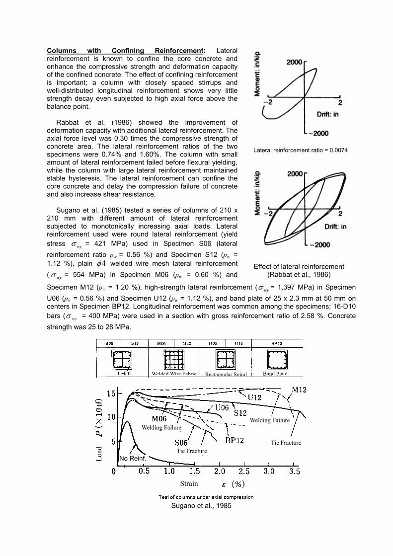
Columns with Confining Reinforcement: Lateral reinforcement is known to confine the core concrete and enhance the compressive strength and deformation capacity of the confined concrete. The effect of confining reinforcement is important; a column with closely spaced stirrups and well-distributed longitudinal reinforcement shows very little strength decay even subjected to high axial force above the balance point.

Rabbat et al. (1986) showed the improvement of deformation capacity with additional lateral reinforcement. The axial force level was 0.30 times the compressive strength of concrete area. The lateral reinforcement ratios of the two specimens were 0.74% and 1.60%. The column with small amount of lateral reinforcement failed before flexural yielding, while the column with large lateral reinforcement maintained stable hysteresis. The lateral reinforcement can confine the core concrete and delay the compression failure of concrete and also increase shear resistance.

Sugano et al. (1985) tested a series of columns of 210 x

210 mm with different amount of lateral reinforcement subjected to monotonically increasing axial loads. Lateral reinforcement used were round lateral reinforcement (yield stress wyσ = 421 MPa) used in Specimen S06 (lateral reinforcement ratio pw = 0.56 %) and Specimen S12 (pw = 1.12 %), plain 4φ welded wire mesh lateral reinforcement ( wyσ = 554 MPa) in Specimen M06 (pw = 0.60 %) and

Specimen M12 (pw = 1.20 %), high-strength lateral reinforcement ( wyσ = 1,397 MPa) in Specimen U06 (pw = 0.56 %) and Specimen U12 (pw = 1.12 %), and band plate of 25 x 2.3 mm at 50 mm on centers in Specimen BP12. Longitudinal reinforcement was common among the specimens; 16-D10 bars ( wyσ = 400 MPa) were used in a section with gross reinforcement ratio of 2.58 %. Concrete strength was 25 to 28 MPa.

Tie FractureTie Fracture

Welding Failure Welding Failure

Strain

No Reinf. Load

Welded Wire Fabric Rectangular Spiral Band Plate

Sugano et al., 1985

Effect of lateral reinforcement

(Rabbat et al., 1986)

Lateral reinforcement ratio = 0.0074

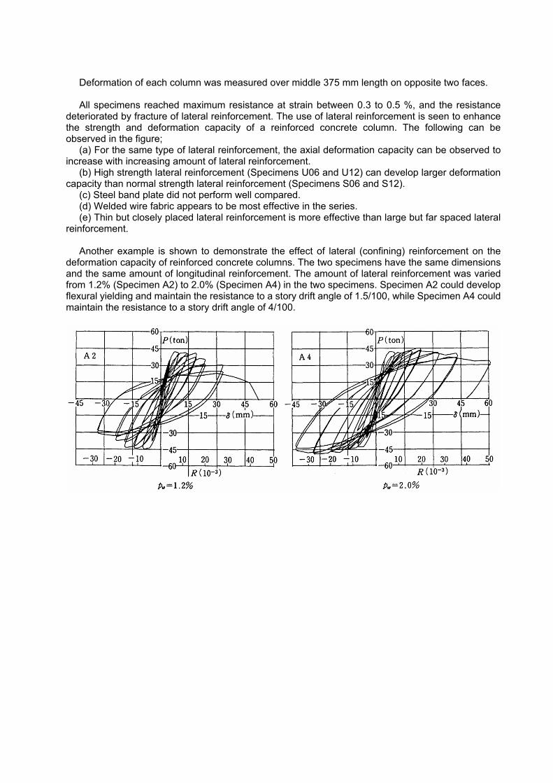
Deformation of each column was measured over middle 375 mm length on opposite two faces. All specimens reached maximum resistance at strain between 0.3 to 0.5 %, and the resistance

deteriorated by fracture of lateral reinforcement. The use of lateral reinforcement is seen to enhance the strength and deformation capacity of a reinforced concrete column. The following can be observed in the figure;

(a) For the same type of lateral reinforcement, the axial deformation capacity can be observed to increase with increasing amount of lateral reinforcement.

(b) High strength lateral reinforcement (Specimens U06 and U12) can develop larger deformation capacity than normal strength lateral reinforcement (Specimens S06 and S12).

(c) Steel band plate did not perform well compared. (d) Welded wire fabric appears to be most effective in the series. (e) Thin but closely placed lateral reinforcement is more effective than large but far spaced lateral

reinforcement. Another example is shown to demonstrate the effect of lateral (confining) reinforcement on the

deformation capacity of reinforced concrete columns. The two specimens have the same dimensions and the same amount of longitudinal reinforcement. The amount of lateral reinforcement was varied from 1.2% (Specimen A2) to 2.0% (Specimen A4) in the two specimens. Specimen A2 could develop flexural yielding and maintain the resistance to a story drift angle of 1.5/100, while Specimen A4 could maintain the resistance to a story drift angle of 4/100.

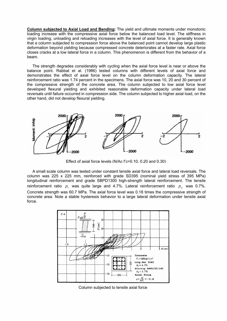
Column subjected to Axial Load and Bending: The yield and ultimate moments under monotonic loading increase with the compressive axial force below the balanced load level. The stiffness in virgin loading, unloading and reloading increases with the level of axial force. It is generally known that a column subjected to compression force above the balanced point cannot develop large plastic deformation beyond yielding because compressed concrete deteriorates at a faster rate. Axial force closes cracks at a low lateral force in a column. This phenomenon is different from the behavior of a beam.

The strength degrades considerably with cycling when the axial force level is near or above the

balance point. Rabbat et al. (1986) tested columns with different levels of axial force and demonstrates the effect of axial force level on the column deformation capacity. The lateral reinforcement ratio was 1.74 percent in the specimens. The axial force was 10, 20 and 30 percent of the compressive strength of the concrete area. The column subjected to low axial force level developed flexural yielding and exhibited reasonable deformation capacity under lateral load reversals until failure occurred in compression side. The column subjected to higher axial load, on the other hand, did not develop flexural yielding.

A small scale column was tested under constant tensile axial force and lateral load reversals. The

column was 225 x 225 mm, reinforced with grade SD395 (nominal yield stress of 395 MPa) longitudinal reinforcement and grade SBPD1300 high-strength lateral reinforcement. The tensile reinforcement ratio tp was quite large and 4.7%. Lateral reinforcement ratio wp was 0.7%. Concrete strength was 60.7 MPa. The axial force level was 0.18 times the compressive strength of concrete area. Note a stable hysteresis behavior to a large lateral deformation under tensile axial force.

Column subjected to tensile axial force

Effect of axial force levels (N/Ac f’c=0.10, 0.20 and 0.30)

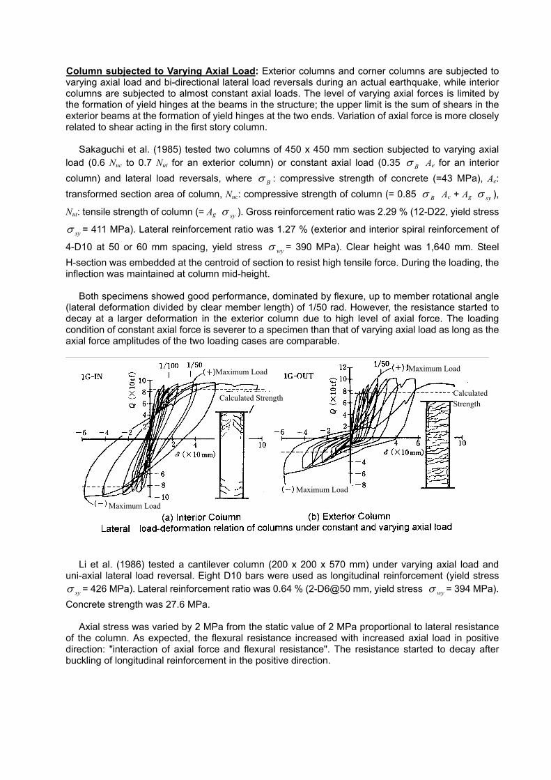
Column subjected to Varying Axial Load: Exterior columns and corner columns are subjected to varying axial load and bi-directional lateral load reversals during an actual earthquake, while interior columns are subjected to almost constant axial loads. The level of varying axial forces is limited by the formation of yield hinges at the beams in the structure; the upper limit is the sum of shears in the exterior beams at the formation of yield hinges at the two ends. Variation of axial force is more closely related to shear acting in the first story column.

Sakaguchi et al. (1985) tested two columns of 450 x 450 mm section subjected to varying axial load (0.6 Nuc to 0.7 Nut for an exterior column) or constant axial load (0.35 Bσ Ae for an interior column) and lateral load reversals, where Bσ : compressive strength of concrete (=43 MPa), Ae: transformed section area of column, Nuc: compressive strength of column (= 0.85 Bσ Ac + Ag syσ ),

Nut: tensile strength of column (= Ag syσ ). Gross reinforcement ratio was 2.29 % (12-D22, yield stress

syσ = 411 MPa). Lateral reinforcement ratio was 1.27 % (exterior and interior spiral reinforcement of

4-D10 at 50 or 60 mm spacing, yield stress wyσ = 390 MPa). Clear height was 1,640 mm. Steel H-section was embedded at the centroid of section to resist high tensile force. During the loading, the inflection was maintained at column mid-height.

Both specimens showed good performance, dominated by flexure, up to member rotational angle

(lateral deformation divided by clear member length) of 1/50 rad. However, the resistance started to decay at a larger deformation in the exterior column due to high level of axial force. The loading condition of constant axial force is severer to a specimen than that of varying axial load as long as the axial force amplitudes of the two loading cases are comparable.

Maximum Load Maximum Load

Calculated Strength Calculated Strength

Maximum Load

Maximum Load

Li et al. (1986) tested a cantilever column (200 x 200 x 570 mm) under varying axial load and

uni-axial lateral load reversal. Eight D10 bars were used as longitudinal reinforcement (yield stress syσ = 426 MPa). Lateral reinforcement ratio was 0.64 % (2-D6@50 mm, yield stress wyσ = 394 MPa).

Concrete strength was 27.6 MPa. Axial stress was varied by 2 MPa from the static value of 2 MPa proportional to lateral resistance

of the column. As expected, the flexural resistance increased with increased axial load in positive direction: "interaction of axial force and flexural resistance". The resistance started to decay after buckling of longitudinal reinforcement in the positive direction.

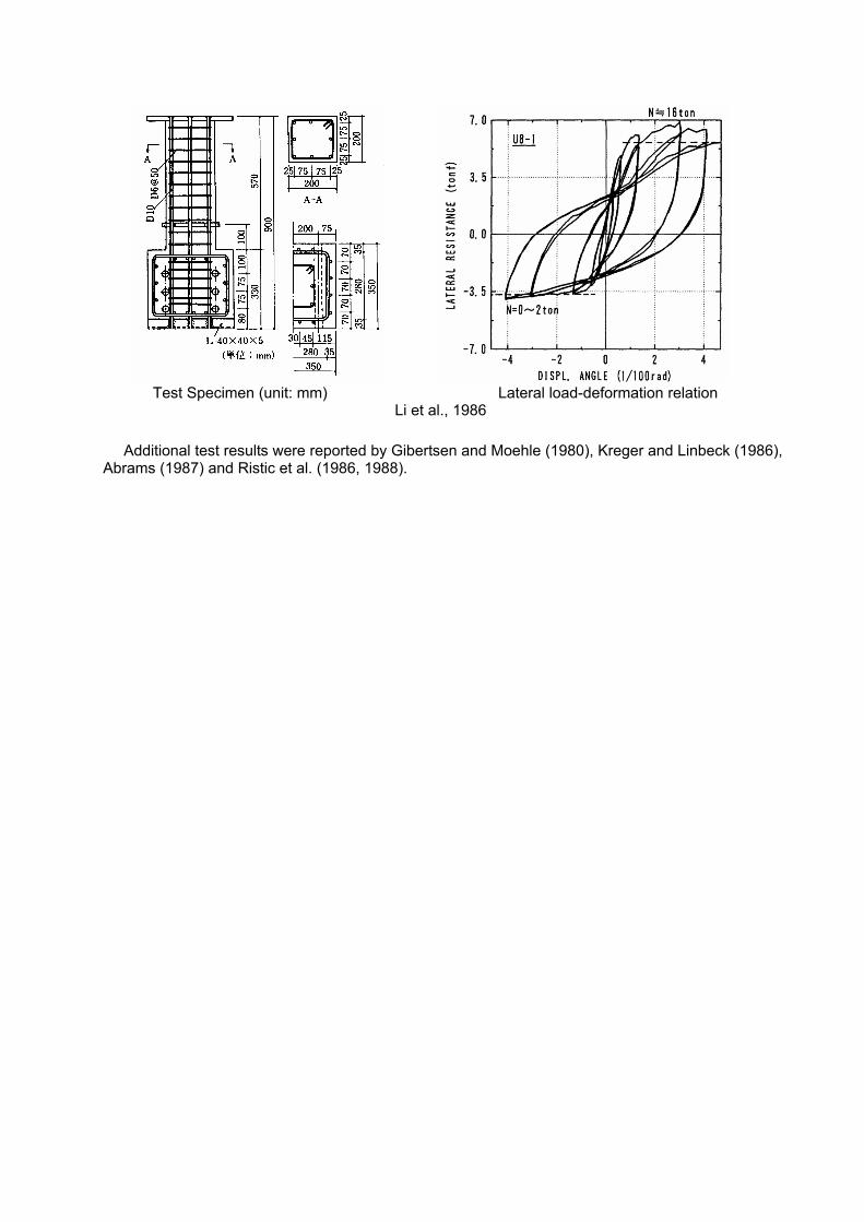
Additional test results were reported by Gibertsen and Moehle (1980), Kreger and Linbeck (1986), Abrams (1987) and Ristic et al. (1986, 1988).

Test Specimen (unit: mm) Lateral load-deformation relation

Li et al., 1986

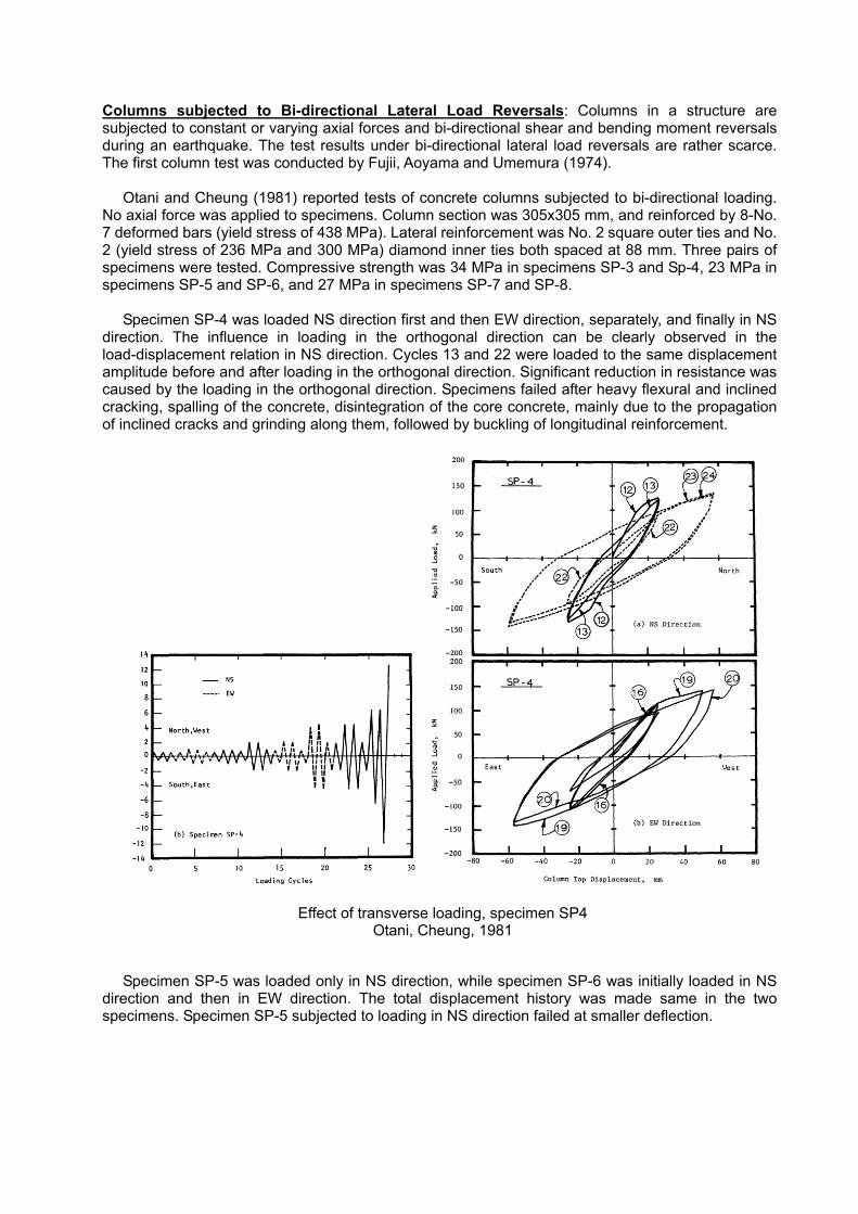
Columns subjected to Bi-directional Lateral Load Reversals: Columns in a structure are subjected to constant or varying axial forces and bi-directional shear and bending moment reversals during an earthquake. The test results under bi-directional lateral load reversals are rather scarce. The first column test was conducted by Fujii, Aoyama and Umemura (1974).

Otani and Cheung (1981) reported tests of concrete columns subjected to bi-directional loading. No axial force was applied to specimens. Column section was 305x305 mm, and reinforced by 8-No. 7 deformed bars (yield stress of 438 MPa). Lateral reinforcement was No. 2 square outer ties and No. 2 (yield stress of 236 MPa and 300 MPa) diamond inner ties both spaced at 88 mm. Three pairs of specimens were tested. Compressive strength was 34 MPa in specimens SP-3 and Sp-4, 23 MPa in specimens SP-5 and SP-6, and 27 MPa in specimens SP-7 and SP-8.

Specimen SP-4 was loaded NS direction first and then EW direction, separately, and finally in NS

direction. The influence in loading in the orthogonal direction can be clearly observed in the load-displacement relation in NS direction. Cycles 13 and 22 were loaded to the same displacement amplitude before and after loading in the orthogonal direction. Significant reduction in resistance was caused by the loading in the orthogonal direction. Specimens failed after heavy flexural and inclined cracking, spalling of the concrete, disintegration of the core concrete, mainly due to the propagation of inclined cracks and grinding along them, followed by buckling of longitudinal reinforcement.

Specimen SP-5 was loaded only in NS direction, while specimen SP-6 was initially loaded in NS direction and then in EW direction. The total displacement history was made same in the two specimens. Specimen SP-5 subjected to loading in NS direction failed at smaller deflection.

Effect of transverse loading, specimen SP4 Otani, Cheung, 1981

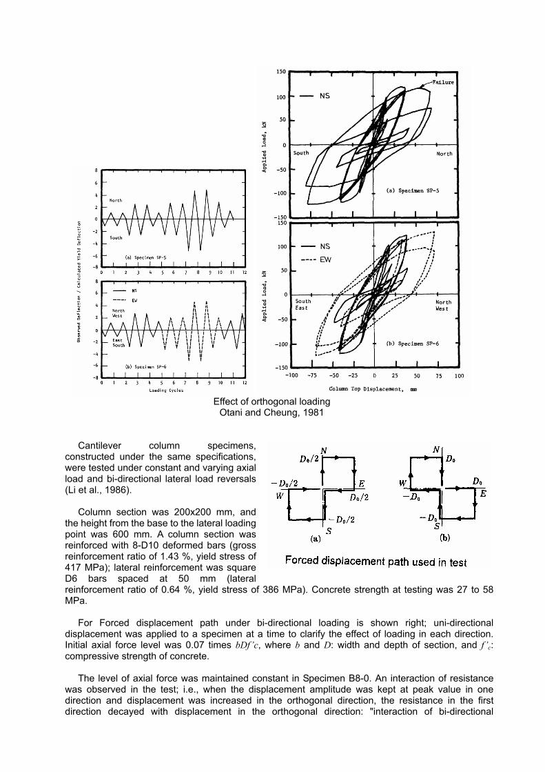
Cantilever column specimens,

constructed under the same specifications, were tested under constant and varying axial load and bi-directional lateral load reversals (Li et al., 1986).

Column section was 200x200 mm, and

the height from the base to the lateral loading point was 600 mm. A column section was reinforced with 8-D10 deformed bars (gross reinforcement ratio of 1.43 %, yield stress of 417 MPa); lateral reinforcement was square D6 bars spaced at 50 mm (lateral reinforcement ratio of 0.64 %, yield stress of 386 MPa). Concrete strength at testing was 27 to 58 MPa.

For Forced displacement path under bi-directional loading is shown right; uni-directional

displacement was applied to a specimen at a time to clarify the effect of loading in each direction. Initial axial force level was 0.07 times bDf’c, where b and D: width and depth of section, and f ’c: compressive strength of concrete.

The level of axial force was maintained constant in Specimen B8-0. An interaction of resistance was observed in the test; i.e., when the displacement amplitude was kept at peak value in one direction and displacement was increased in the orthogonal direction, the resistance in the first direction decayed with displacement in the orthogonal direction: "interaction of bi-directional

Effect of orthogonal loading

Otani and Cheung, 1981

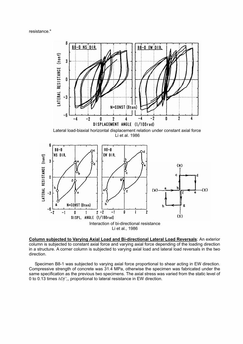
resistance."

Column subjected to Varying Axial Load and Bi-directional Lateral Load Reversals: An exterior column is subjected to constant axial force and varying axial force depending of the loading direction in a structure. A corner column is subjected to varying axial load and lateral load reversals in the two direction.

Specimen B8-1 was subjected to varying axial force proportional to shear acting in EW direction. Compressive strength of concrete was 31.4 MPa, otherwise the specimen was fabricated under the same specification as the previous two specimens. The axial stress was varied from the static level of 0 to 0.13 times bDf’c, proportional to lateral resistance in EW direction.

Interaction of bi-directional resistance Li et al., 1986

Lateral load-biaxial horizontal displacement relation under constant axial forceLi et al. 1986

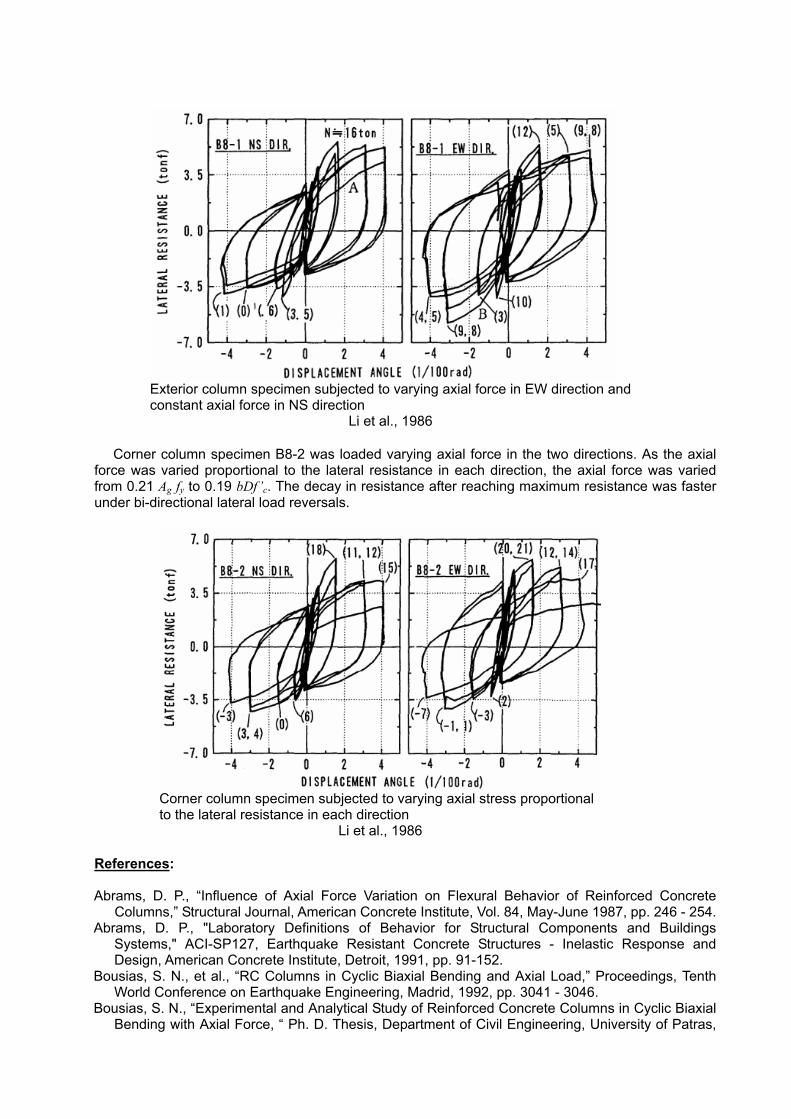
Corner column specimen B8-2 was loaded varying axial force in the two directions. As the axial

force was varied proportional to the lateral resistance in each direction, the axial force was varied from 0.21 Ag fy to 0.19 bDf’c. The decay in resistance after reaching maximum resistance was faster under bi-directional lateral load reversals.

References: Abrams, D. P., “Influence of Axial Force Variation on Flexural Behavior of Reinforced Concrete

Columns,” Structural Journal, American Concrete Institute, Vol. 84, May-June 1987, pp. 246 - 254. Abrams, D. P., "Laboratory Definitions of Behavior for Structural Components and Buildings

Systems," ACI-SP127, Earthquake Resistant Concrete Structures - Inelastic Response and Design, American Concrete Institute, Detroit, 1991, pp. 91-152.

Bousias, S. N., et al., “RC Columns in Cyclic Biaxial Bending and Axial Load,” Proceedings, Tenth World Conference on Earthquake Engineering, Madrid, 1992, pp. 3041 - 3046.

Bousias, S. N., “Experimental and Analytical Study of Reinforced Concrete Columns in Cyclic Biaxial Bending with Axial Force, “ Ph. D. Thesis, Department of Civil Engineering, University of Patras,

Corner column specimen subjected to varying axial stress proportional to the lateral resistance in each direction

Li et al., 1986

Exterior column specimen subjected to varying axial force in EW direction and constant axial force in NS direction

Li et al., 1986

Greece, 1993. Fujii, S., “Study on Reinforced Concrete Columns subjected to Biaxial Flexure (in Japanese),” M. eng.

Thesis, Department of Architecture, University of Tokyo, 1974. Gibertsen, N. and J. P. Moehle, “Experimental Study of Small Scale R/C Columns subjected to Axial

Load and Shear Reversals,” Structural Research Series No. 481, Department of Civil Engineering, University of Illinois at Urbana, 1980.

Higashi, Y., M. Ohkubo and M. Ohtsuka, “Influence of Loading Excursions on Restoring Force Characteristics and Failure Modes of Reinforced Concrete Columns,” Paper No. 11-23, Sixth World Conference on Earthquake Engineering, New Delhi, January 1977.

Kreger, M., and L. Linbeck, “Behavior of Reinforced Concrete Columns subjected to Lateral and Axial Loading Reversals,” Proceedings, Third U.S. National Conference on Earthquake Engineering, Charleston, South Carolina, Vol. “, pp. 1475 - 1486, 1986.

Li, K.-N., et al., "Behavior of Reinforced Concrete Columns subjected to Varying Axial Load and Bi-directional Horizontal Earthquake Loads (in Japanese)," Proceedings, Eighth Annual Conference, Japan Concrete Institute, pp. 489-492, 1986.

Low, S., and J. P. Moehle, “Experimental Study of Reinforced Concrete Columns subjected to Multi-axial Cyclic Loading,” Earthquake Engineering Research Center, University of California at Berkeley, EERC Report 87-14,1987.

Otani, S, "Nonlinear Dynamic Analysis of Reinforced Concrete Building Structures," Canadian Journal of Civil Engineering, Vol. 7, National Research Council of Canada, pp. 333-344, 1980.

Otani, S., and V. W.-T. Cheung, “Behavior of Reinforced Concrete Columns under Biaxial Lateral Load Reversals, - (II) Test without Axial Loads,” Department of Civil Engineering Publication 81-02, University of Toronto, February 1981, 127 pp.

Rabbat, B., et al., “Seismic Behavior of Light-weight and Normal-weight Concrete Columns,” Journal, American Concrete Institute, Vol. 83, Jan.-Feb. 1986, pp. 69 - 78..

Ristic, D., et al., “Effect of Variation of Axial Forces to Hysteretic Earthquake Response of Reinforced Concrete Structures,” Proceedings, Eighth European Conference on Earthquake engineering, Lisbon, Vol. 4, 7.4, 1986, pp. 49 - 56.

Ristic, D., et al., “Inelastic Stress-strain based Seismic Response Prediction of RC Structures considering Dynamically Varying Axial Forces,” Proceedings, Ninth World Conference on Earthquake Engineering, Tokyo-Kyoto, 1988, Vol. VI, pp. 531 - 536.

Saatcioglu, M., "Modeling Hysteretic Force-Deformation Relations for Reinforced Concrete Elements," ACI SP-127, Earthquake-Resistant Concrete Structures - Inelastic Response and Design, American Concrete Institute, Detroit, 1991, pp. 153-198.

Saatcioglu, M., and G. Azcebe, “Response of Reinforced Concrete Columns to Simulated Seismic Loading,” Structural Journal, American Concrete Institute, Vol. 86, Jan.-Feb. 1989, pp. 3 12.

Sakaguchi, N., et al., "Study on Structural Characteristics of High-rise Reinforced Concrete Residential Buildings (Part 2: Strength Test of Columns) (in Japanese)," Summary Report, Annual Meeting, Architectural Institute of Japan, Structures 2, pp. 153-154, October 1985.

Sugano, S., et al., "Experimental Study on High-rise Reinforced Concrete Buildings (Part 1: Outline of Study and Compression Test of Columns) (in Japanese)," Summary Report, Annual Meeting, Architectural Institute of Japan, Structures 2, pp. 145-146, October 1985.

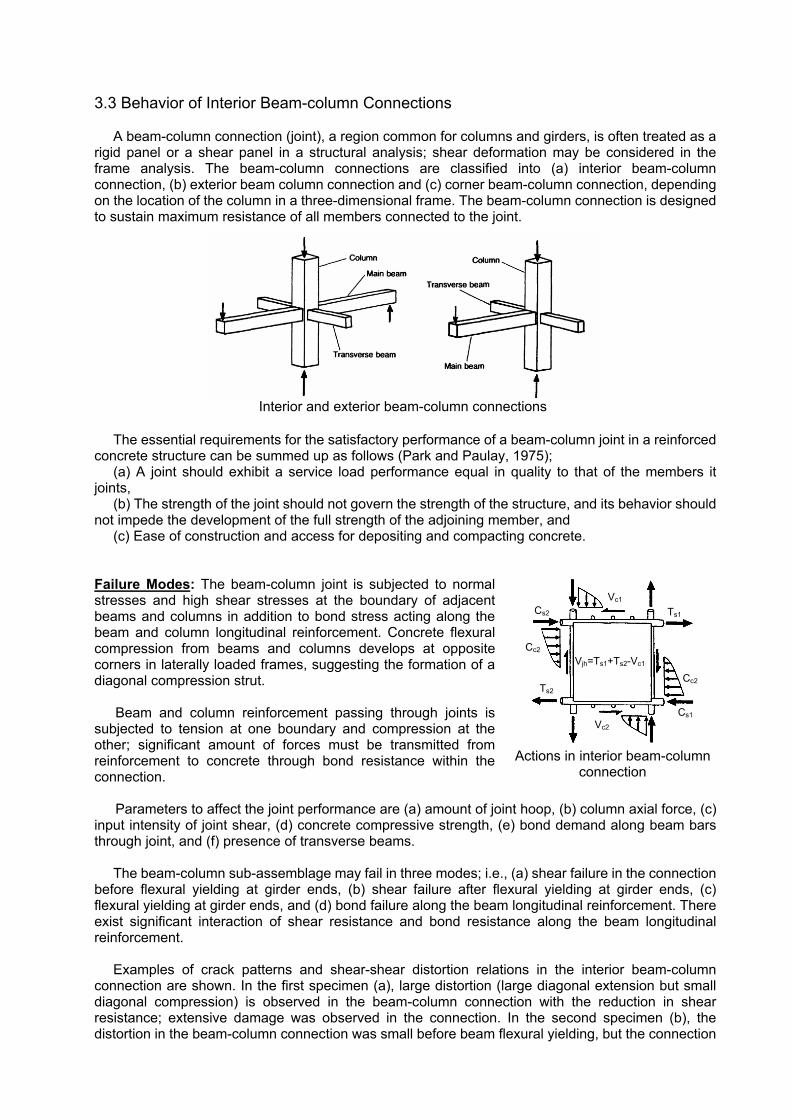
3.3 Behavior of Interior Beam-column Connections

A beam-column connection (joint), a region common for columns and girders, is often treated as a rigid panel or a shear panel in a structural analysis; shear deformation may be considered in the frame analysis. The beam-column connections are classified into (a) interior beam-column connection, (b) exterior beam column connection and (c) corner beam-column connection, depending on the location of the column in a three-dimensional frame. The beam-column connection is designed to sustain maximum resistance of all members connected to the joint.

The essential requirements for the satisfactory performance of a beam-column joint in a reinforced

concrete structure can be summed up as follows (Park and Paulay, 1975); (a) A joint should exhibit a service load performance equal in quality to that of the members it

joints, (b) The strength of the joint should not govern the strength of the structure, and its behavior should

not impede the development of the full strength of the adjoining member, and (c) Ease of construction and access for depositing and compacting concrete.

Failure Modes: The beam-column joint is subjected to normal stresses and high shear stresses at the boundary of adjacent beams and columns in addition to bond stress acting along the beam and column longitudinal reinforcement. Concrete flexural compression from beams and columns develops at opposite corners in laterally loaded frames, suggesting the formation of a diagonal compression strut.

Beam and column reinforcement passing through joints is subjected to tension at one boundary and compression at the other; significant amount of forces must be transmitted from reinforcement to concrete through bond resistance within the connection.

Parameters to affect the joint performance are (a) amount of joint hoop, (b) column axial force, (c) input intensity of joint shear, (d) concrete compressive strength, (e) bond demand along beam bars through joint, and (f) presence of transverse beams.

The beam-column sub-assemblage may fail in three modes; i.e., (a) shear failure in the connection before flexural yielding at girder ends, (b) shear failure after flexural yielding at girder ends, (c) flexural yielding at girder ends, and (d) bond failure along the beam longitudinal reinforcement. There exist significant interaction of shear resistance and bond resistance along the beam longitudinal reinforcement.

Examples of crack patterns and shear-shear distortion relations in the interior beam-column

connection are shown. In the first specimen (a), large distortion (large diagonal extension but small diagonal compression) is observed in the beam-column connection with the reduction in shear resistance; extensive damage was observed in the connection. In the second specimen (b), the distortion in the beam-column connection was small before beam flexural yielding, but the connection

Interior and exterior beam-column connections

Ts1

Cs1

Cc2

Cs2

Ts2

Cc2

Vc1

Vc2

Vjh=Ts1+Ts2-Vc1

Actions in interior beam-column

connection

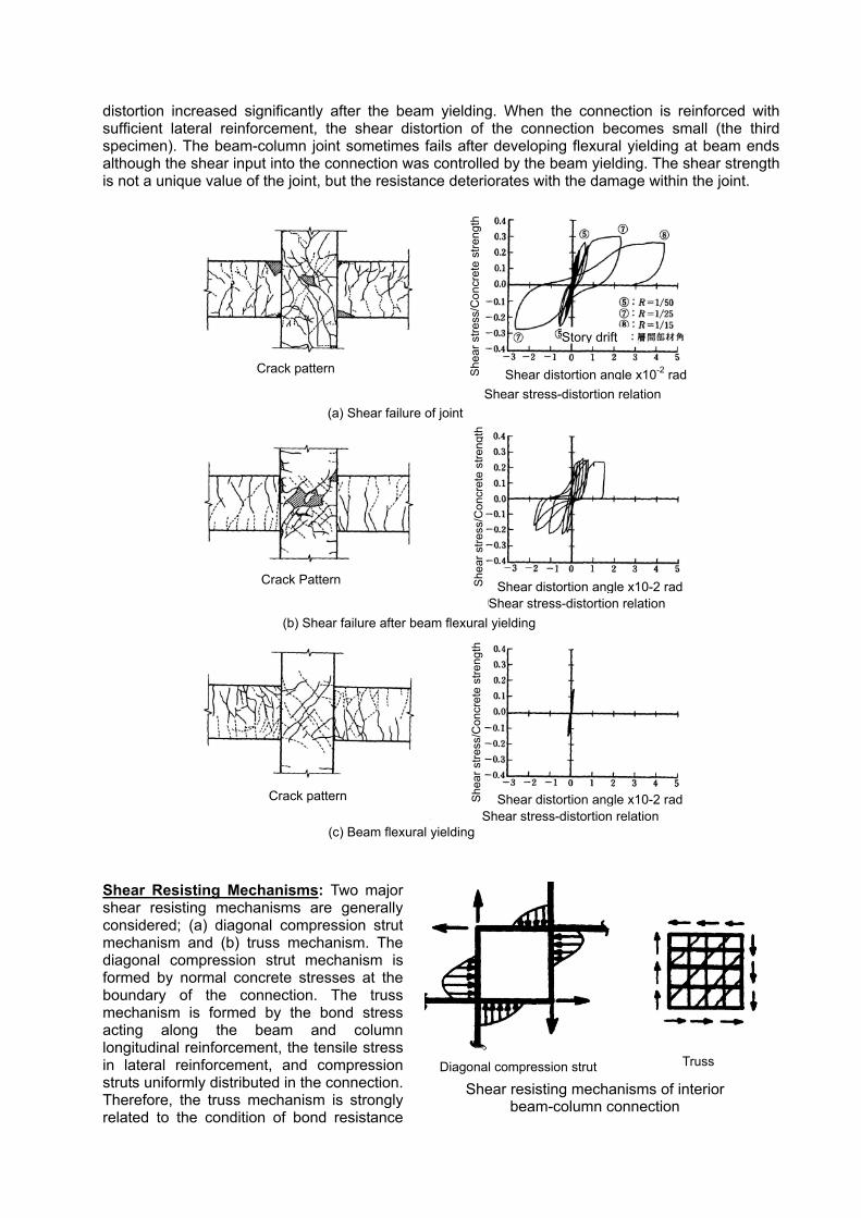
distortion increased significantly after the beam yielding. When the connection is reinforced with sufficient lateral reinforcement, the shear distortion of the connection becomes small (the third specimen). The beam-column joint sometimes fails after developing flexural yielding at beam ends although the shear input into the connection was controlled by the beam yielding. The shear strength is not a unique value of the joint, but the resistance deteriorates with the damage within the joint.

Crack pattern

(a) Shear failure of joint Shear stress-distortion relation

Shear distortion angle x10-2 rad

Crack Pattern

Story drift

She

ar s

tress

/Con

cret

e st

reng

th

(b) Shear failure after beam flexural yieldingShear stress-distortion relation

Shear distortion angle x10-2 rad She

ar s

tress

/Con

cret

e st

reng

th

Crack pattern Shear distortion angle x10-2 rad Shear stress-distortion relation

She

ar s

tress

/Con

cret

e st

reng

th

(c) Beam flexural yielding Shear Resisting Mechanisms: Two major shear resisting mechanisms are generally considered; (a) diagonal compression strut mechanism and (b) truss mechanism. The diagonal compression strut mechanism is formed by normal concrete stresses at the boundary of the connection. The truss mechanism is formed by the bond stress acting along the beam and column longitudinal reinforcement, the tensile stress in lateral reinforcement, and compression struts uniformly distributed in the connection. Therefore, the truss mechanism is strongly related to the condition of bond resistance

Diagonal compression strut Truss

Shear resisting mechanisms of interior beam-column connection

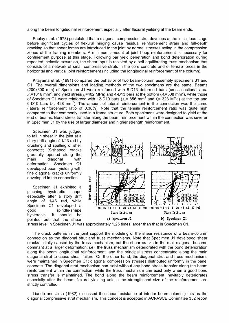
along the beam longitudinal reinforcement especially after flexural yielding at the beam ends.

Paulay et al. (1978) postulated that a diagonal compression strut develops at the initial load stage before significant cycles of flexural hinging cause residual reinforcement strain and full-depth cracking so that shear forces are introduced to the joint by normal stresses acting in the compression zones of the framing members. A minimum amount of joint hoop reinforcement is necessary for confinement purpose at this stage. Following bar yield penetration and bond deterioration during repeated inelastic excursion, the shear input is resisted by a self-equilibrating truss mechanism that consists of a network of small compressive struts in the core concrete and of tensile forces in the horizontal and vertical joint reinforcement (including the longitudinal reinforcement of the column).

Kitayama et al. (1991) compared the behavior of two beam-column assembly specimens J1 and C1. The overall dimensions and loading methods of the two specimens are the same. Beams (200x300 mm) of Specimen J1 were reinforced with 8-D13 deformed bars (cross sectional area As=1016 mm2, and yield stress fy=402 MPa) and 4-D13 bars at the bottom (As=508 mm2), while those of Specimen C1 were reinforced with 12-D10 bars (As= 856 mm2 and fy= 323 MPa) at the top and 6-D10 bars (As=428 mm2). The amount of lateral reinforcement in the connection was the same (lateral reinforcement ratio of 0.38%). Note that the tensile reinforcement ratio was quite high compared to that commonly used in a frame structure. Both specimens were designed to yield at the end of beams. Bond stress transfer along the beam reinforcement within the connection was severer in Specimen J1 by the use of larger diameter and higher strength reinforcement.

Specimen J1 was judged

to fail in shear in the joint at a story drift angle of 1/23 rad by crushing and spalling of shell concrete; X-shaped cracks gradually opened along the main diagonal with deformation. Specimen C1 developed beam yielding with fine diagonal cracks uniformly developed in the connection.

Specimen J1 exhibited a

pinching hysteretic shape especially after a story drift angle of 1/46 rad, while Specimen C1 developed a good spindle-shape hysteresis. It should be pointed out that the shear stress level in Specimen J1 was approximately 1.25 times larger than that in Specimen C1.

The crack patterns in the joint support the modeling of the shear resistance of a beam-column

connection as the diagonal strut and truss mechanisms. Note that Specimen J1 developed shear cracks initially caused by the truss mechanism, but the shear cracks in the mail diagonal became dominant at a larger deformation; i.e., the truss mechanism deteriorated with the bond deterioration along the beam longitudinal reinforcement, and the principal stress concentrated along the main diagonal strut to cause shear failure. On the other hand, the diagonal strut and truss mechanisms were maintained in Specimen C1; diagonal compression stresses distributed uniformly in the panel concrete. The diagonal strut mechanism can exist without any bond stress transfer along the beam reinforcement within the connection, while the truss mechanism can exist only when a good bond stress transfer is maintained. The bond along the beam reinforcement inevitably deteriorates especially after the beam flexural yielding unless the strength and size of the reinforcement are strictly controlled.

Liande and Jirsa (1982) discussed the shear resistance of interior beam-column joints as the diagonal compressive strut mechanism. This concept is accepted in ACI-ASCE Committee 352 report

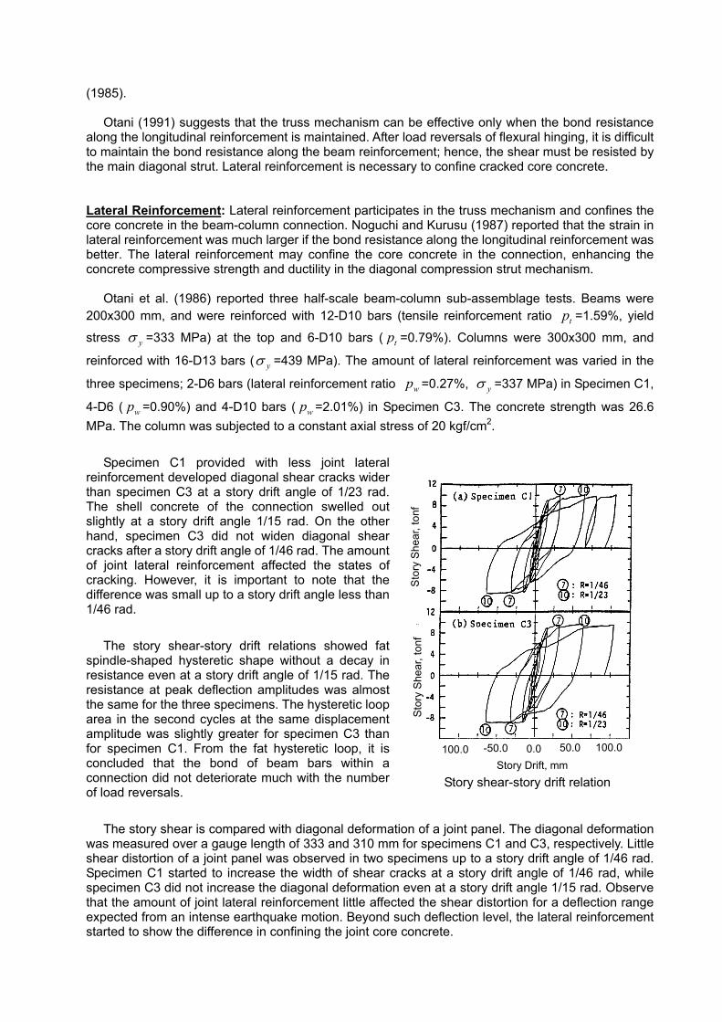
(1985).

Otani (1991) suggests that the truss mechanism can be effective only when the bond resistance along the longitudinal reinforcement is maintained. After load reversals of flexural hinging, it is difficult to maintain the bond resistance along the beam reinforcement; hence, the shear must be resisted by the main diagonal strut. Lateral reinforcement is necessary to confine cracked core concrete. Lateral Reinforcement: Lateral reinforcement participates in the truss mechanism and confines the core concrete in the beam-column connection. Noguchi and Kurusu (1987) reported that the strain in lateral reinforcement was much larger if the bond resistance along the longitudinal reinforcement was better. The lateral reinforcement may confine the core concrete in the connection, enhancing the concrete compressive strength and ductility in the diagonal compression strut mechanism.

Otani et al. (1986) reported three half-scale beam-column sub-assemblage tests. Beams were 200x300 mm, and were reinforced with 12-D10 bars (tensile reinforcement ratio tp =1.59%, yield

stress yσ =333 MPa) at the top and 6-D10 bars ( tp =0.79%). Columns were 300x300 mm, and

reinforced with 16-D13 bars ( yσ =439 MPa). The amount of lateral reinforcement was varied in the

three specimens; 2-D6 bars (lateral reinforcement ratio wp =0.27%, yσ =337 MPa) in Specimen C1,

4-D6 ( wp =0.90%) and 4-D10 bars ( wp =2.01%) in Specimen C3. The concrete strength was 26.6 MPa. The column was subjected to a constant axial stress of 20 kgf/cm2.

Specimen C1 provided with less joint lateral

reinforcement developed diagonal shear cracks wider than specimen C3 at a story drift angle of 1/23 rad. The shell concrete of the connection swelled out slightly at a story drift angle 1/15 rad. On the other hand, specimen C3 did not widen diagonal shear cracks after a story drift angle of 1/46 rad. The amount of joint lateral reinforcement affected the states of cracking. However, it is important to note that the difference was small up to a story drift angle less than 1/46 rad.

The story shear-story drift relations showed fat

spindle-shaped hysteretic shape without a decay in resistance even at a story drift angle of 1/15 rad. The resistance at peak deflection amplitudes was almost the same for the three specimens. The hysteretic loop area in the second cycles at the same displacement amplitude was slightly greater for specimen C3 than for specimen C1. From the fat hysteretic loop, it is concluded that the bond of beam bars within a connection did not deteriorate much with the number of load reversals.

The story shear is compared with diagonal deformation of a joint panel. The diagonal deformation

was measured over a gauge length of 333 and 310 mm for specimens C1 and C3, respectively. Little shear distortion of a joint panel was observed in two specimens up to a story drift angle of 1/46 rad. Specimen C1 started to increase the width of shear cracks at a story drift angle of 1/46 rad, while specimen C3 did not increase the diagonal deformation even at a story drift angle 1/15 rad. Observe that the amount of joint lateral reinforcement little affected the shear distortion for a deflection range expected from an intense earthquake motion. Beyond such deflection level, the lateral reinforcement started to show the difference in confining the joint core concrete.

0.0 50.0 100.0-50.0100.0Story Drift, mm

Sto

ry S

hear

, ton

f S

tory

She

ar, t

onf

Story shear-story drift relation

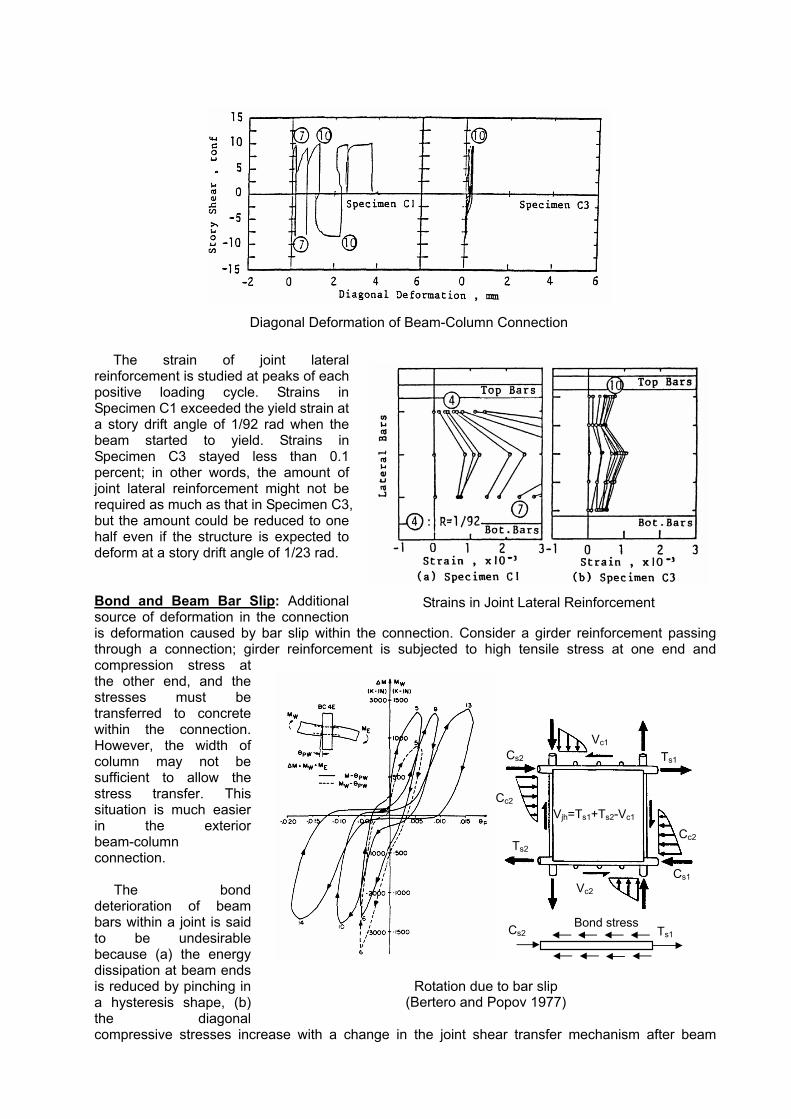
The strain of joint lateral

reinforcement is studied at peaks of each positive loading cycle. Strains in Specimen C1 exceeded the yield strain at a story drift angle of 1/92 rad when the beam started to yield. Strains in Specimen C3 stayed less than 0.1 percent; in other words, the amount of joint lateral reinforcement might not be required as much as that in Specimen C3, but the amount could be reduced to one half even if the structure is expected to deform at a story drift angle of 1/23 rad. Bond and Beam Bar Slip: Additional source of deformation in the connection is deformation caused by bar slip within the connection. Consider a girder reinforcement passing through a connection; girder reinforcement is subjected to high tensile stress at one end and compression stress at the other end, and the stresses must be transferred to concrete within the connection. However, the width of column may not be sufficient to allow the stress transfer. This situation is much easier in the exterior beam-column connection.

The bond deterioration of beam bars within a joint is said to be undesirable because (a) the energy dissipation at beam ends is reduced by pinching in a hysteresis shape, (b) the diagonal compressive stresses increase with a change in the joint shear transfer mechanism after beam

Ts1

Cs1

Cc2

Cs2

Ts2

Cc2

Vc1

Vc2

Vjh=Ts1+Ts2-Vc1

Ts1 Cs2Bond stress

Rotation due to bar slip

(Bertero and Popov 1977)

Diagonal Deformation of Beam-Column Connection

Strains in Joint Lateral Reinforcement

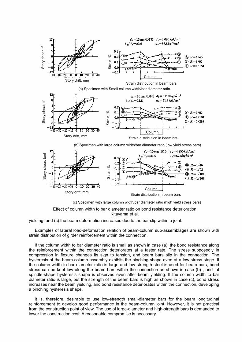
yielding, and (c) the beam deformation increases due to the bar slip within a joint. Examples of lateral load-deformation relation of beam-column sub-assemblages are shown with

strain distribution of girder reinforcement within the connection.

If the column width to bar diameter ratio is small as shown in case (a), the bond resistance along the reinforcement within the connection deteriorates at a faster rate. The stress supposedly in compression in flexure changes its sign to tension, and beam bars slip in the connection. The hysteresis of the beam-column assembly exhibits the pinching shape even at a low stress stage. If the column width to bar diameter ratio is large and low strength steel is used for beam bars, bond stress can be kept low along the beam bars within the connection as shown in case (b) , and fat spindle-shape hysteresis shape is observed even after beam yielding. If the column width to bar diameter ratio is large, but the strength of the beam bars is high as shown in case (c), bond stress increases near the beam yielding, and bond resistance deteriorates within the connection, developing a pinching hysteresis shape.

It is, therefore, desirable to use low-strength small-diameter bars for the beam longitudinal

reinforcement to develop good performance in the beam-column joint. However, it is not practical from the construction point of view. The use of large-diameter and high-strength bars is demanded to lower the construction cost. A reasonable compromise is necessary.

Story drift, mm Strain distribution in beam bars

Column

(a) Specimen with Small column width/bar diameter ratio

Sto

ry s

hear

, tf

(b) Specimen with large column width/bar diameter ratio (low yield stress bars)

ColumnStrain distribution in beam brs Story drift, mm

Sto

ry s

hear

, tf

Stra

in, %

S

train

, %

Strain distribution in beam bars Column

Story drift, mm

Sto

ry s

hear

, ton

f

Stra

in,%

(c) Specimen with large column width/bar diameter ratio (high yield stress bars)

Effect of column width to bar diameter ratio on bond resistance deterioration Kitayama et al.

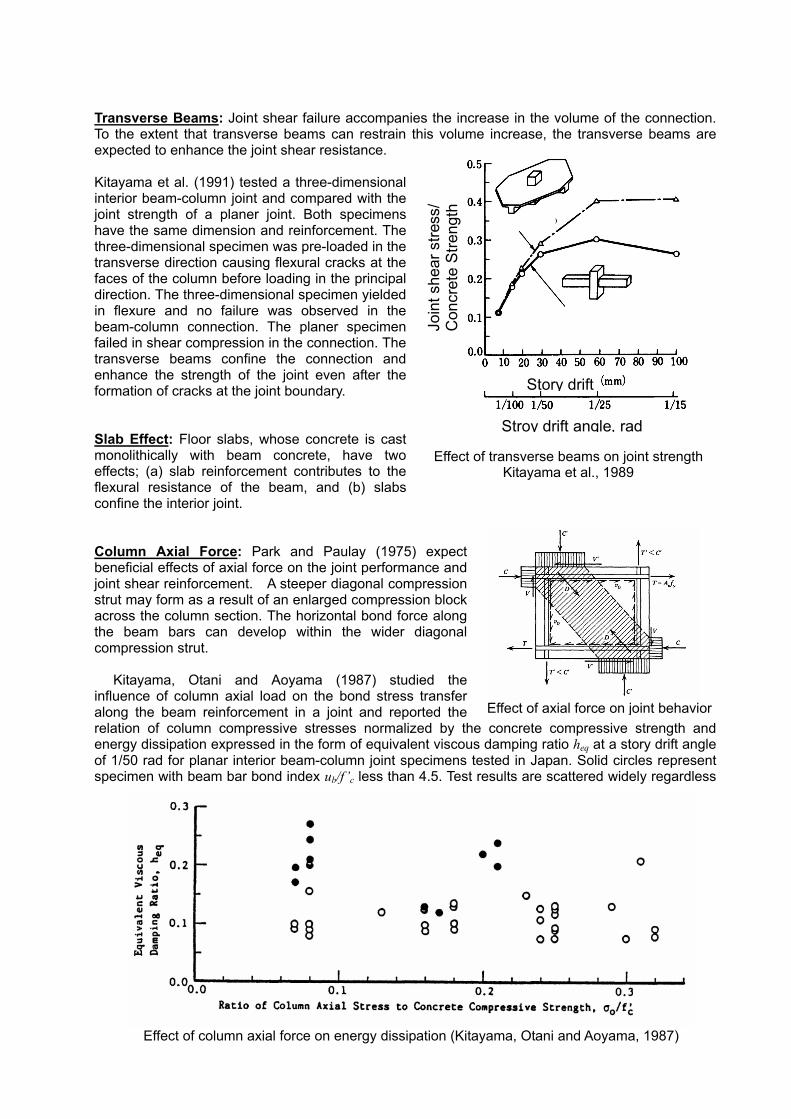
Transverse Beams: Joint shear failure accompanies the increase in the volume of the connection. To the extent that transverse beams can restrain this volume increase, the transverse beams are expected to enhance the joint shear resistance. Kitayama et al. (1991) tested a three-dimensional interior beam-column joint and compared with the joint strength of a planer joint. Both specimens have the same dimension and reinforcement. The three-dimensional specimen was pre-loaded in the transverse direction causing flexural cracks at the faces of the column before loading in the principal direction. The three-dimensional specimen yielded in flexure and no failure was observed in the beam-column connection. The planer specimen failed in shear compression in the connection. The transverse beams confine the connection and enhance the strength of the joint even after the formation of cracks at the joint boundary. Slab Effect: Floor slabs, whose concrete is cast monolithically with beam concrete, have two effects; (a) slab reinforcement contributes to the flexural resistance of the beam, and (b) slabs confine the interior joint. Column Axial Force: Park and Paulay (1975) expect beneficial effects of axial force on the joint performance and joint shear reinforcement. A steeper diagonal compression strut may form as a result of an enlarged compression block across the column section. The horizontal bond force along the beam bars can develop within the wider diagonal compression strut.

Kitayama, Otani and Aoyama (1987) studied the influence of column axial load on the bond stress transfer along the beam reinforcement in a joint and reported the relation of column compressive stresses normalized by the concrete compressive strength and energy dissipation expressed in the form of equivalent viscous damping ratio heq at a story drift angle of 1/50 rad for planar interior beam-column joint specimens tested in Japan. Solid circles represent specimen with beam bar bond index ub/f’c less than 4.5. Test results are scattered widely regardless

Story drift

Stroy drift angle, rad Jo

int s

hear

stre

ss/

Con

cret

e St

reng

th

Effect of transverse beams on joint strength

Kitayama et al., 1989

Effect of axial force on joint behavior

Effect of column axial force on energy dissipation (Kitayama, Otani and Aoyama, 1987)

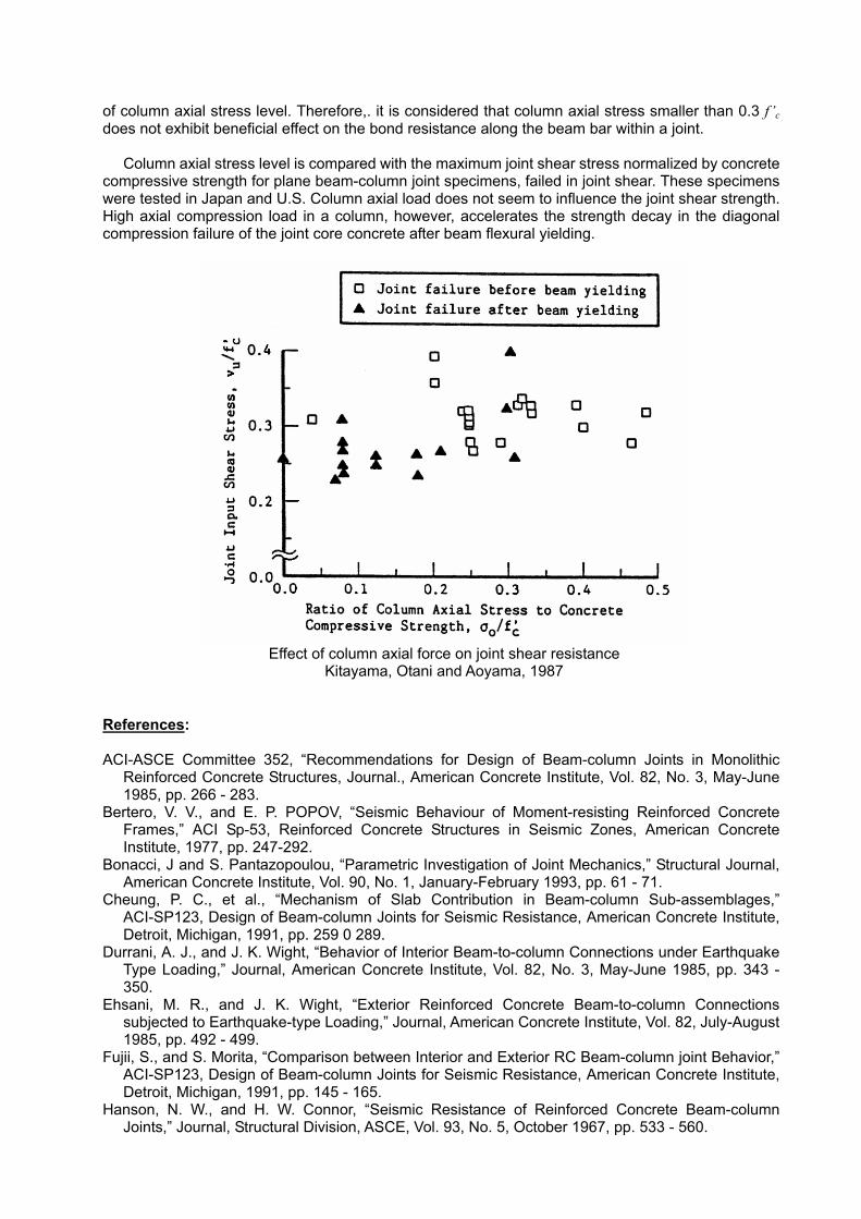
of column axial stress level. Therefore,. it is considered that column axial stress smaller than 0.3 f ’c does not exhibit beneficial effect on the bond resistance along the beam bar within a joint.

Column axial stress level is compared with the maximum joint shear stress normalized by concrete

compressive strength for plane beam-column joint specimens, failed in joint shear. These specimens were tested in Japan and U.S. Column axial load does not seem to influence the joint shear strength. High axial compression load in a column, however, accelerates the strength decay in the diagonal compression failure of the joint core concrete after beam flexural yielding.

References: ACI-ASCE Committee 352, “Recommendations for Design of Beam-column Joints in Monolithic

Reinforced Concrete Structures, Journal., American Concrete Institute, Vol. 82, No. 3, May-June 1985, pp. 266 - 283.

Bertero, V. V., and E. P. POPOV, “Seismic Behaviour of Moment-resisting Reinforced Concrete Frames,” ACI Sp-53, Reinforced Concrete Structures in Seismic Zones, American Concrete Institute, 1977, pp. 247-292.

Bonacci, J and S. Pantazopoulou, “Parametric Investigation of Joint Mechanics,” Structural Journal, American Concrete Institute, Vol. 90, No. 1, January-February 1993, pp. 61 - 71.

Cheung, P. C., et al., “Mechanism of Slab Contribution in Beam-column Sub-assemblages,” ACI-SP123, Design of Beam-column Joints for Seismic Resistance, American Concrete Institute, Detroit, Michigan, 1991, pp. 259 0 289.

Durrani, A. J., and J. K. Wight, “Behavior of Interior Beam-to-column Connections under Earthquake Type Loading,” Journal, American Concrete Institute, Vol. 82, No. 3, May-June 1985, pp. 343 - 350.

Ehsani, M. R., and J. K. Wight, “Exterior Reinforced Concrete Beam-to-column Connections subjected to Earthquake-type Loading,” Journal, American Concrete Institute, Vol. 82, July-August 1985, pp. 492 - 499.

Fujii, S., and S. Morita, “Comparison between Interior and Exterior RC Beam-column joint Behavior,” ACI-SP123, Design of Beam-column Joints for Seismic Resistance, American Concrete Institute, Detroit, Michigan, 1991, pp. 145 - 165.

Hanson, N. W., and H. W. Connor, “Seismic Resistance of Reinforced Concrete Beam-column Joints,” Journal, Structural Division, ASCE, Vol. 93, No. 5, October 1967, pp. 533 - 560.

Effect of column axial force on joint shear resistance

Kitayama, Otani and Aoyama, 1987

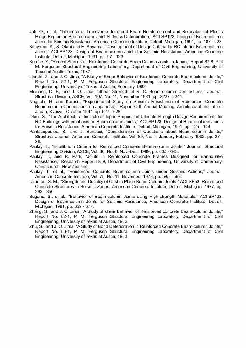
Joh, O., et al., “Influence of Transverse Joint and Beam Reinforcement and Relocation of Plastic Hinge Region on Beam-column Joint Stiffness Deterioration,” ACI-SP123, Design of Beam-column Joints for Seismic Resistance, American Concrete Institute, Detroit, Michigan, 1991, pp. 187 - 223.

Kitayama, K., S. Otani and H. Aoyama, “Development of Design Criteria for RC Interior Beam-column Joints,” ACI-SP123, Design of Beam-column Joints for Seismic Resistance, American Concrete Institute, Detroit, Michigan, 1991, pp. 97 - 123.

Kurose, Y., “Recent Studies on Reinforced Concrete Beam Column Joints in Japan,” Report 87-8, Phil M. Ferguson Structural Engineering Laboratory, Department of Civil Engineering, University of Texas at Austin, Texas, 1987.

Liande, Z., and J. O. Jirsa, “A Study of Shear Behavior of Reinforced Concrete Beam-column Joints,” Report No. 82-1, P. M. Ferguson Structural Engineering Laboratory, Department of Civil Engineering, University of Texas at Austin, February 1982.

Meinheit, D. F., and J. O. Jirsa, “Shear Strength of R. C. Beam-column Connections,” Journal, Structural Division, ASCE, Vol. 107, No. 11, November 1981, pp. 2227 -2244.

Noguchi, H. and Kurusu, “Experimental Study on Seismic Resistance of Reinforced Concrete Beam-column Connections (in Japanese),” Report C-II, Annual Meeting, Architectural Institute of Japan, Kyusyu, October 1997, pp. 627 - 628.

Otani, S., “The Architectural Institute of Japan Proposal of Ultimate Strength Design Requirements for RC Buildings with emphasis on Beam-column Joints,” ACI-SP123, Design of Beam-column Joints for Seismic Resistance, American Concrete Institute, Detroit, Michigan, 1991, pp. 125 - 144.

Pantazopoulou, S., and J. Bonacci, “Consideration of Questions about Beam-column Joints,” Structural Journal, American Concrete Institute, Vol. 89, No. 1, January-February 1992, pp. 27 - 36.

Paulay, T., “Equilibrium Criteria for Reinforced Concrete Beam-column Joints,” Journal, Structural Engineering Division, ASCE, Vol. 86, No. 6, Nov.-Dec. 1989, pp. 635 - 643.

Paulay, T., and R. Park, “Joints in Reinforced Concrete Frames Designed for Earthquake Resistance,” Research Report 84-9, Department of Civil Engineering, University of Canterbury, Christchurch, New Zealand.

Paulay, T., et al., “Reinforced Concrete Beam-column Joints under Seismic Actions,” Journal, American Concrete Institute, Vol. 75, No. 11. November 1978, pp. 585 - 593.

Uzumeri, S. M., “Strength and Ductility of Cast in Place Beam Column Joints,” ACI-SP53, Reinforced Concrete Structures in Seismic Zones, American Concrete Institute, Detroit, Michigan, 1977, pp. 293 - 350.

Sugano, S., et al., “Behavior of Beam-column Joints using High-strength Materials,” ACI-SP123, Design of Beam-column Joints for Seismic Resistance, American Concrete Institute, Detroit, Michigan, 1991, pp. 359 - 377.

Zhang, S., and J. O. Jirsa, “A Study of shear Behavior of Reinforced concrete Beam-column Joints,” Report No. 82-1, P. M. Ferguson Structural Engineering Laboratory, Department of Civil Engineering, University of Texas at Austin, 1982.

Zhu, S., and J. O. Jirsa, “A Study of Bond Deterioration in Reinforced Concrete Beam-column Joints,” Report No. 83-1, P. M. Ferguson Structural Engineering Laboratory, Department of Civil Engineering, University of Texas at Austin, 1983.

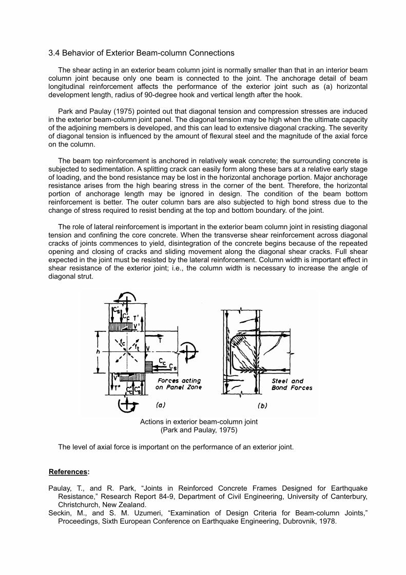
3.4 Behavior of Exterior Beam-column Connections The shear acting in an exterior beam column joint is normally smaller than that in an interior beam

column joint because only one beam is connected to the joint. The anchorage detail of beam longitudinal reinforcement affects the performance of the exterior joint such as (a) horizontal development length, radius of 90-degree hook and vertical length after the hook.

Park and Paulay (1975) pointed out that diagonal tension and compression stresses are induced

in the exterior beam-column joint panel. The diagonal tension may be high when the ultimate capacity of the adjoining members is developed, and this can lead to extensive diagonal cracking. The severity of diagonal tension is influenced by the amount of flexural steel and the magnitude of the axial force on the column.

The beam top reinforcement is anchored in relatively weak concrete; the surrounding concrete is subjected to sedimentation. A splitting crack can easily form along these bars at a relative early stage of loading, and the bond resistance may be lost in the horizontal anchorage portion. Major anchorage resistance arises from the high bearing stress in the corner of the bent. Therefore, the horizontal portion of anchorage length may be ignored in design. The condition of the beam bottom reinforcement is better. The outer column bars are also subjected to high bond stress due to the change of stress required to resist bending at the top and bottom boundary. of the joint.

The role of lateral reinforcement is important in the exterior beam column joint in resisting diagonal

tension and confining the core concrete. When the transverse shear reinforcement across diagonal cracks of joints commences to yield, disintegration of the concrete begins because of the repeated opening and closing of cracks and sliding movement along the diagonal shear cracks. Full shear expected in the joint must be resisted by the lateral reinforcement. Column width is important effect in shear resistance of the exterior joint; i.e., the column width is necessary to increase the angle of diagonal strut.

The level of axial force is important on the performance of an exterior joint.

References:

Paulay, T., and R. Park, “Joints in Reinforced Concrete Frames Designed for Earthquake Resistance,” Research Report 84-9, Department of Civil Engineering, University of Canterbury, Christchurch, New Zealand.

Seckin, M., and S. M. Uzumeri, “Examination of Design Criteria for Beam-column Joints,” Proceedings, Sixth European Conference on Earthquake Engineering, Dubrovnik, 1978.

Actions in exterior beam-column joint

(Park and Paulay, 1975)

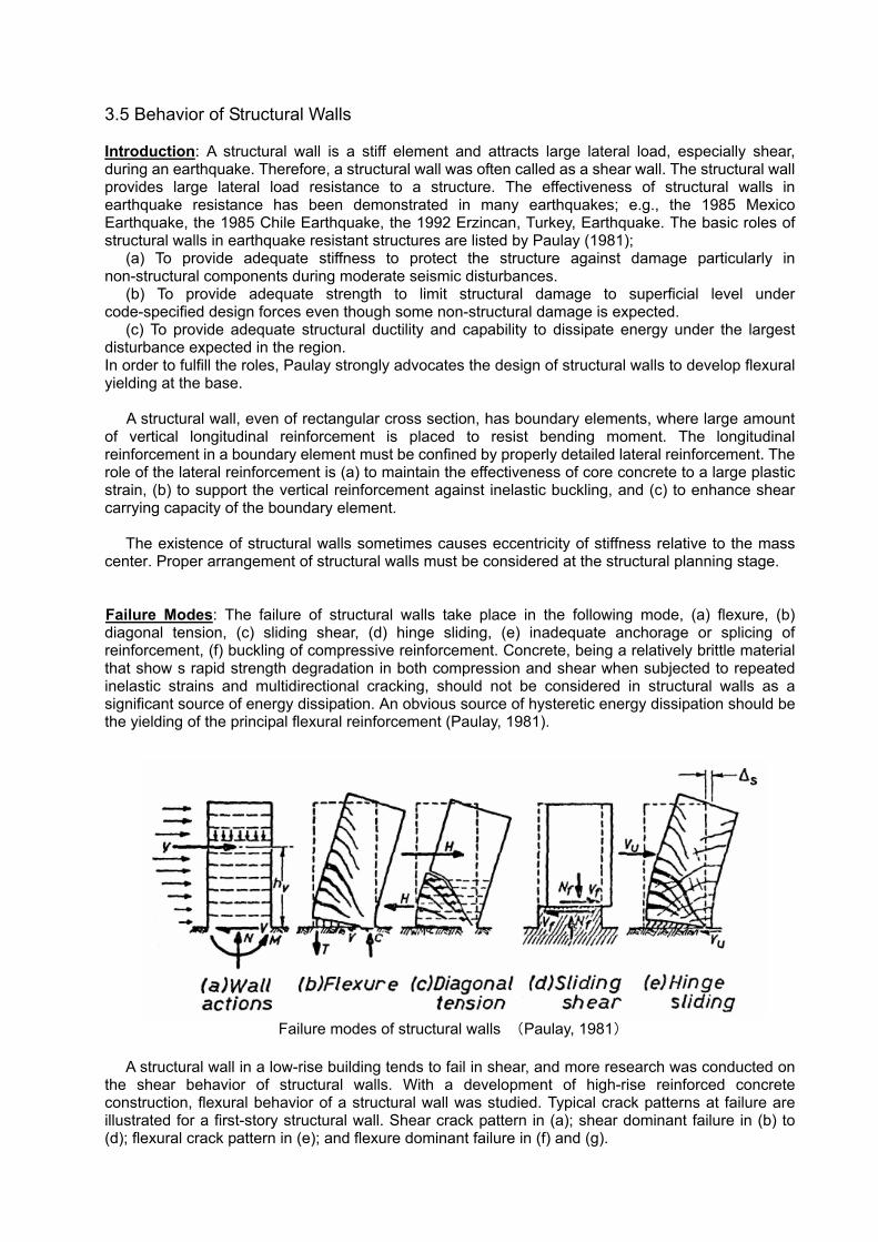
3.5 Behavior of Structural Walls

Introduction: A structural wall is a stiff element and attracts large lateral load, especially shear, during an earthquake. Therefore, a structural wall was often called as a shear wall. The structural wall provides large lateral load resistance to a structure. The effectiveness of structural walls in earthquake resistance has been demonstrated in many earthquakes; e.g., the 1985 Mexico Earthquake, the 1985 Chile Earthquake, the 1992 Erzincan, Turkey, Earthquake. The basic roles of structural walls in earthquake resistant structures are listed by Paulay (1981);

(a) To provide adequate stiffness to protect the structure against damage particularly in non-structural components during moderate seismic disturbances.

(b) To provide adequate strength to limit structural damage to superficial level under code-specified design forces even though some non-structural damage is expected.

(c) To provide adequate structural ductility and capability to dissipate energy under the largest disturbance expected in the region. In order to fulfill the roles, Paulay strongly advocates the design of structural walls to develop flexural yielding at the base.

A structural wall, even of rectangular cross section, has boundary elements, where large amount of vertical longitudinal reinforcement is placed to resist bending moment. The longitudinal reinforcement in a boundary element must be confined by properly detailed lateral reinforcement. The role of the lateral reinforcement is (a) to maintain the effectiveness of core concrete to a large plastic strain, (b) to support the vertical reinforcement against inelastic buckling, and (c) to enhance shear carrying capacity of the boundary element.

The existence of structural walls sometimes causes eccentricity of stiffness relative to the mass center. Proper arrangement of structural walls must be considered at the structural planning stage.

Failure Modes: The failure of structural walls take place in the following mode, (a) flexure, (b) diagonal tension, (c) sliding shear, (d) hinge sliding, (e) inadequate anchorage or splicing of reinforcement, (f) buckling of compressive reinforcement. Concrete, being a relatively brittle material that show s rapid strength degradation in both compression and shear when subjected to repeated inelastic strains and multidirectional cracking, should not be considered in structural walls as a significant source of energy dissipation. An obvious source of hysteretic energy dissipation should be the yielding of the principal flexural reinforcement (Paulay, 1981).

A structural wall in a low-rise building tends to fail in shear, and more research was conducted on

the shear behavior of structural walls. With a development of high-rise reinforced concrete construction, flexural behavior of a structural wall was studied. Typical crack patterns at failure are illustrated for a first-story structural wall. Shear crack pattern in (a); shear dominant failure in (b) to (d); flexural crack pattern in (e); and flexure dominant failure in (f) and (g).

Failure modes of structural walls （Paulay, 1981）

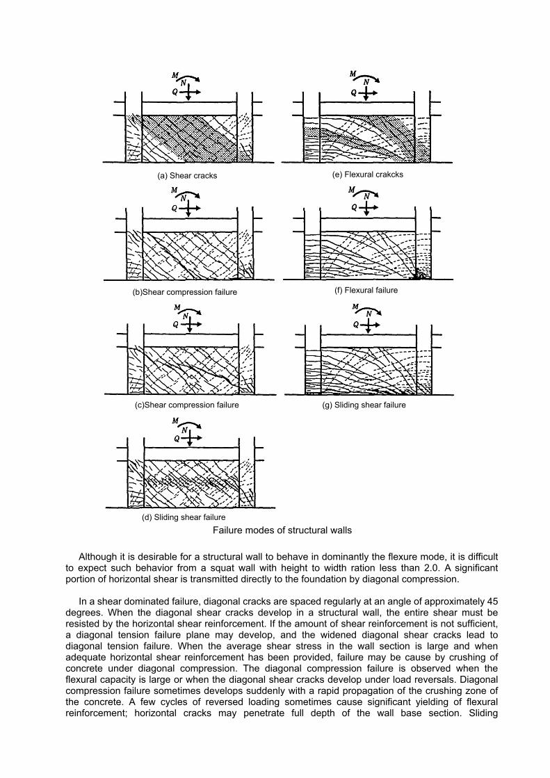
Although it is desirable for a structural wall to behave in dominantly the flexure mode, it is difficult

to expect such behavior from a squat wall with height to width ration less than 2.0. A significant portion of horizontal shear is transmitted directly to the foundation by diagonal compression.

In a shear dominated failure, diagonal cracks are spaced regularly at an angle of approximately 45 degrees. When the diagonal shear cracks develop in a structural wall, the entire shear must be resisted by the horizontal shear reinforcement. If the amount of shear reinforcement is not sufficient, a diagonal tension failure plane may develop, and the widened diagonal shear cracks lead to diagonal tension failure. When the average shear stress in the wall section is large and when adequate horizontal shear reinforcement has been provided, failure may be cause by crushing of concrete under diagonal compression. The diagonal compression failure is observed when the flexural capacity is large or when the diagonal shear cracks develop under load reversals. Diagonal compression failure sometimes develops suddenly with a rapid propagation of the crushing zone of the concrete. A few cycles of reversed loading sometimes cause significant yielding of flexural reinforcement; horizontal cracks may penetrate full depth of the wall base section. Sliding

(a) Shear cracks (e) Flexural crakcks

(b)Shear compression failure (f) Flexural failure

(c)Shear compression failure (g) Sliding shear failure

(d) Sliding shear failure

Failure modes of structural walls

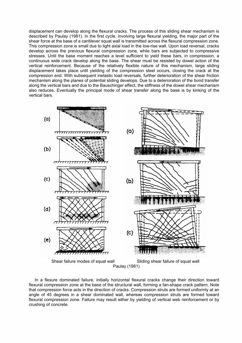
displacement can develop along the flexural cracks. The process of this sliding shear mechanism is described by Paulay (1981). In the first cycle, involving large flexural yielding, the major part of the shear force at the base of a cantilever squat wall is transmitted across the flexural compression zone. This compression zone is small due to light axial load in the low-rise wall. Upon load reversal, cracks develop across the previous flexural compression zone, while bars are subjected to compressive stresses. Until the base moment reaches a level sufficient to yield these bars, in compression, a continuous wide crack develop along the base. The shear must be resisted by dowel action of the vertical reinforcement. Because of the relatively flexible nature of this mechanism, large sliding displacement takes place until yielding of the compression steel occurs, closing the crack at the compression end. With subsequent inelastic load reversals, further deterioration of the shear friction mechanism along the planes of potential sliding develops. Due to a deterioration of the bond transfer along the vertical bars and due to the Bauschinger effect, the stiffness of the dowel shear mechanism also reduces. Eventually the principal mode of shear transfer along the base is by kinking of the vertical bars.

In a flexure dominated failure, initially horizontal flexural cracks change their direction toward

flexural compression zone at the base of the structural wall, forming a fan-shape crack pattern. Note that compression force acts in the direction of cracks. Compression struts are formed uniformly at an angle of 45 degrees in a shear dominated wall, whereas compression struts are formed toward flexural compression zone. Failure may result either by yielding of vertical web reinforcement or by crushing of concrete.

Shear failure modes of squat wall Sliding shear failure of squat wall

Paulay (1981)

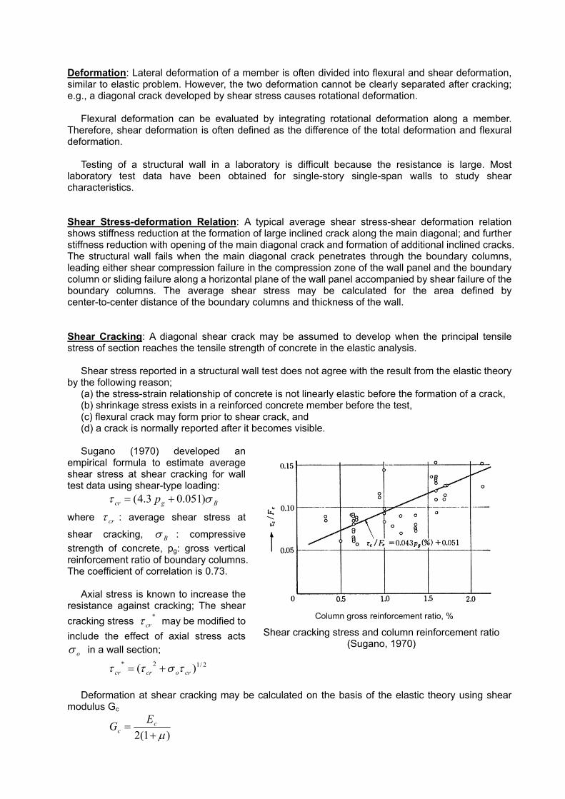
Deformation: Lateral deformation of a member is often divided into flexural and shear deformation, similar to elastic problem. However, the two deformation cannot be clearly separated after cracking; e.g., a diagonal crack developed by shear stress causes rotational deformation.

Flexural deformation can be evaluated by integrating rotational deformation along a member.

Therefore, shear deformation is often defined as the difference of the total deformation and flexural deformation.

Testing of a structural wall in a laboratory is difficult because the resistance is large. Most

laboratory test data have been obtained for single-story single-span walls to study shear characteristics. Shear Stress-deformation Relation: A typical average shear stress-shear deformation relation shows stiffness reduction at the formation of large inclined crack along the main diagonal; and further stiffness reduction with opening of the main diagonal crack and formation of additional inclined cracks. The structural wall fails when the main diagonal crack penetrates through the boundary columns, leading either shear compression failure in the compression zone of the wall panel and the boundary column or sliding failure along a horizontal plane of the wall panel accompanied by shear failure of the boundary columns. The average shear stress may be calculated for the area defined by center-to-center distance of the boundary columns and thickness of the wall. Shear Cracking: A diagonal shear crack may be assumed to develop when the principal tensile stress of section reaches the tensile strength of concrete in the elastic analysis.

Shear stress reported in a structural wall test does not agree with the result from the elastic theory by the following reason;

(a) the stress-strain relationship of concrete is not linearly elastic before the formation of a crack, (b) shrinkage stress exists in a reinforced concrete member before the test, (c) flexural crack may form prior to shear crack, and (d) a crack is normally reported after it becomes visible. Sugano (1970) developed an

empirical formula to estimate average shear stress at shear cracking for wall test data using shear-type loading:

Bgcr p στ )051.03.4( +=

where crτ : average shear stress at

shear cracking, Bσ : compressive strength of concrete, pg: gross vertical reinforcement ratio of boundary columns. The coefficient of correlation is 0.73.

Axial stress is known to increase the resistance against cracking; The shear cracking stress *

crτ may be modified to include the effect of axial stress acts

oσ in a wall section; 2/12* )( crocrcr τσττ +=

Deformation at shear cracking may be calculated on the basis of the elastic theory using shear

modulus Gc

)1(2 µ+= c

cEG

Column gross reinforcement ratio, %

Shear cracking stress and column reinforcement ratio(Sugano, 1970)

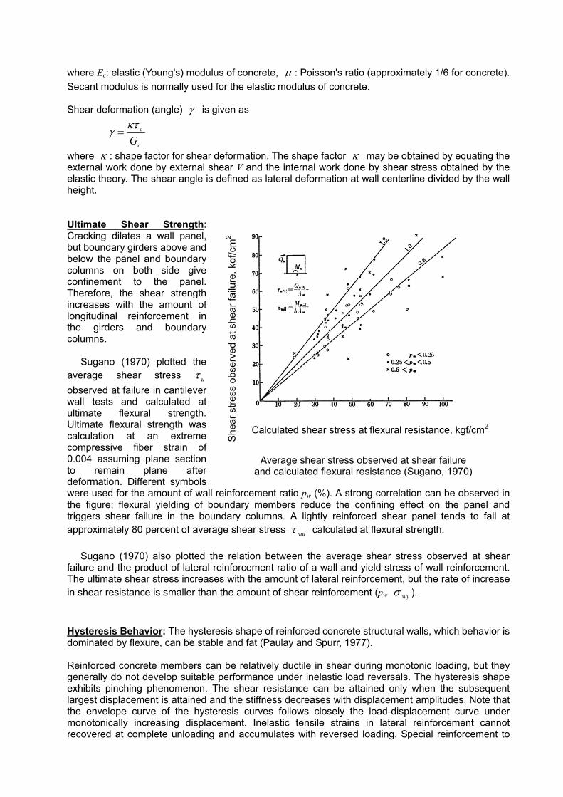
where Ec: elastic (Young's) modulus of concrete, µ : Poisson's ratio (approximately 1/6 for concrete). Secant modulus is normally used for the elastic modulus of concrete. Shear deformation (angle) γ is given as

c

c

Gκτγ =

where κ : shape factor for shear deformation. The shape factor κ may be obtained by equating the external work done by external shear V and the internal work done by shear stress obtained by the elastic theory. The shear angle is defined as lateral deformation at wall centerline divided by the wall height. Ultimate Shear Strength: Cracking dilates a wall panel, but boundary girders above and below the panel and boundary columns on both side give confinement to the panel. Therefore, the shear strength increases with the amount of longitudinal reinforcement in the girders and boundary columns.

Sugano (1970) plotted the average shear stress uτ observed at failure in cantilever wall tests and calculated at ultimate flexural strength. Ultimate flexural strength was calculation at an extreme compressive fiber strain of 0.004 assuming plane section to remain plane after deformation. Different symbols were used for the amount of wall reinforcement ratio pw (%). A strong correlation can be observed in the figure; flexural yielding of boundary members reduce the confining effect on the panel and triggers shear failure in the boundary columns. A lightly reinforced shear panel tends to fail at approximately 80 percent of average shear stress muτ calculated at flexural strength.

Sugano (1970) also plotted the relation between the average shear stress observed at shear

failure and the product of lateral reinforcement ratio of a wall and yield stress of wall reinforcement. The ultimate shear stress increases with the amount of lateral reinforcement, but the rate of increase in shear resistance is smaller than the amount of shear reinforcement (pw wyσ ). Hysteresis Behavior: The hysteresis shape of reinforced concrete structural walls, which behavior is dominated by flexure, can be stable and fat (Paulay and Spurr, 1977). Reinforced concrete members can be relatively ductile in shear during monotonic loading, but they generally do not develop suitable performance under inelastic load reversals. The hysteresis shape exhibits pinching phenomenon. The shear resistance can be attained only when the subsequent largest displacement is attained and the stiffness decreases with displacement amplitudes. Note that the envelope curve of the hysteresis curves follows closely the load-displacement curve under monotonically increasing displacement. Inelastic tensile strains in lateral reinforcement cannot recovered at complete unloading and accumulates with reversed loading. Special reinforcement to

Calculated shear stress at flexural resistance, kgf/cm2

She

ar s

tress

obs

erve

d at

she

ar fa

ilure

, kgf

/cm

2

Average shear stress observed at shear failure

and calculated flexural resistance (Sugano, 1970)

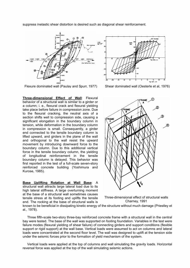
suppress inelastic shear distortion is desired such as diagonal shear reinforcement.

Three-dimensional Effect of Wall: Flexural behavior of a structural wall is similar to a girder or a column; i. e., flexural crack and flexural yielding take place before failure in compression zone. Due to the flexural cracking, the neutral axis of a section shifts well to compression side, causing a significant elongation in the boundary column in tension, while deformation in the boundary column in compression is small. Consequently, a girder end connected to the tensile boundary column is lifted upward, and girders in the plane of the wall and orthogonal to the wall resist the upward movement by introducing downward force to the boundary column. Due to this additional vertical force in the tensile boundary column, the yielding of longitudinal reinforcement in the tensile boundary column is delayed. This behavior was first reported in the test of a full-scale seven-story reinforced concrete building (Yoshimura and Kurose, 1985). Base Uplifting Rotation at Wall Base: A structural wall attracts large lateral load due to its high lateral stiffness. A large overturning moment at the base of a structural wall sometimes causes tensile stress at its footing and uplifts the tensile end. The rocking at the base of structural walls is known to be beneficial in dissipating kinetic energy of the structure without much damage (Priestley et al., 1978).

Three fifth-scale two-story three-bay reinforced concrete frame with a structural wall in the central bay were tested. The base of the wall was supported on footing foundation. Variables in the test were failure modes (flexural yielding of shear failure) of connecting girders and support conditions (flexible support or rigid support) at the wall base. Vertical loads were assumed to act on columns and lateral loads were concentrated at the second floor level. The wall was designed to uplift at the tension side under the seismic forces prior to the formation of yield mechanism of the system.

Vertical loads were applied at the top of columns and wall simulating the gravity loads. Horizontal

reversal force was applied at the top of the wall simulating seismic actions.

Flexure dominated wall (Paulay and Spurr, 1977) Shear dominated wall (Oesterle et al, 1976)

Three-dimensional effect of structural walls

Charney, 1991

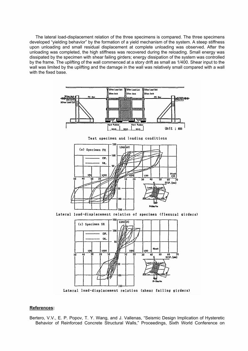
The lateral load-displacement relation of the three specimens is compared. The three specimens

developed “yielding behavior” by the formation of a yield mechanism of the system. A steep stiffness upon unloading and small residual displacement at complete unloading was observed. After the unloading was completed, the high stiffness was recovered during the reloading. Small energy was dissipated by the specimen with shear failing girders; energy dissipation of the system was controlled by the frame. The uplifting of the wall commenced at a story drift as small as 1/400. Shear input to the wall was limited by the uplifting and the damage in the wall was relatively small compared with a wall with the fixed base.

References: Bertero, V.V., E. P. Popov, T. Y. Wang, and J. Vallenas, “Seismic Design Implication of Hysteretic

Behavior of Reinforced Concrete Structural Walls,” Proceedings, Sixth World Conference on

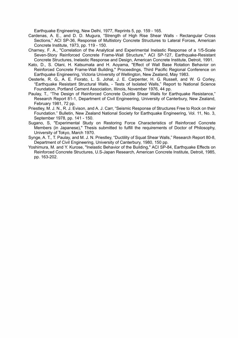
Earthquake Engineering, New Delhi, 1977, Reprints 5, pp. 159 - 165. Cardenas, A. E., and D. D. Mugura, “Strength of High Rise Shear Walls - Rectangular Cross

Sections,” ACI SP-36, Response of Multistory Concrete Structures to Lateral Forces, American Concrete Institute, 1973, pp. 119 - 150.

Charney, F. A., "Correlation of the Analytical and Experimental Inelastic Response of a 1/5-Scale Seven-Story Reinforced Concrete Frame-Wall Structure," ACI SP-127, Earthquake-Resistant Concrete Structures, Inelastic Response and Design, American Concrete Institute, Detroit, 1991.

Kato, D., S. Otani, H. Katsumata and H. Aoyama, "Effect of Wall Base Rotation Behavior on Reinforced Concrete Frame-Wall Building," Proceedings, Third Pacific Regional Conference on Earthquake Engineering, Victoria University of Wellington, New Zealand, May 1983.

Oesterle, R. G., A. E. Fiorato, L. S. Johal, J. E. Carpenter, H. G. Russell, and W. G Corley, “Earthquake Resistant Structural Walls, - Tests of Isolated Walls,” Report to National Science Foundation, Portland Cement Association, Illinois, November 1976, 44 pp.

Paulay, T., “The Design of Reinforced Concrete Ductile Shear Walls for Earthquake Resistance,” Research Report 81-1, Department of Civil Engineering, University of Canterbury, New Zealand, February 1981, 72 pp.

Priestley, M. J. N., R. J. Evison, and A. J. Carr, “Seismic Response of Structures Free to Rock on their Foundation.” Bulletin, New Zealand National Society for Earthquake Engineering, Vol. 11, No. 3, September 1978, pp. 141 - 150.

Sugano, S, "Experimental Study on Restoring Force Characteristics of Reinforced Concrete Members (in Japanese)," Thesis submitted to fulfill the requirements of Doctor of Philosophy, University of Tokyo, March 1970.

Synge, A. T., T. Paulay, and M. J. N. Priestley, “Ductility of Squat Shear Walls,” Research Report 80-8, Department of Civil Engineering, University of Canterbury, 1980, 150 pp.

Yoshimura, M. and Y. Kurose, "Inelastic Behavior of the Building," ACI SP-84, Earthquake Effects on Reinforced Concrete Structures, U.S-Japan Research, American Concrete Institute, Detroit, 1985, pp. 163-202.

Home Assignment No. 2

2001-10-24 Otani, S.

Discuss the following topics on typical behavior of reinforced concrete members: (1) Load-deflection relation of a beam with different amount of longitudinal reinforcement at the top

and at the bottom, typically seen in a T-shaped beam Reference: Ma, S. M., V. V. Bertero and E. P. Popov, "Experimental and Analytical Studies of the

Hysteretic Behavior of Reinforced Concrete Members under Bidirectional Reversed Lateral Loading," Report No. EERC 76-2, University of California at Berkeley, 1976.

(2) Effect of slab on the stiffness and flexural resistance of a beam. Reference: French, C. W., and A. Boroojerdi, "Contribution of RC Floor Slabs in Resisting Lateral

Loads," Journal, Structural Engineering, ASCE, Vol. 115, No. 1, January 1989, pp. 1-18. (3) Role of compressive reinforcement on flexural resistance and deformation capacity.

1

Chapter 4 Analysis of Reinforced Concrete Members

The minimum modeling element of nonlinear analysis of a structure can be selected as (a) material level modeling (Finite Element Method), (b) member level modeling (frame modeling), (c) story level modeling (mass-and-spring modeling), and (d) one-degree-of-freedom model for an entire structure. The finite element method (FEM) is used for material level modeling. The story level modeling by a mass-and-stick model was extensively used to understand the overall behavior of a structure. Recent capacity and demand spectra method idealizes a structure by a single-degree-of-freedom system.

The FEM has been developed for a half century, and is popularly used in the analysis of reinforced concrete member and sub-assemblage even in a nonlinear range to failure. The nonlinear FEM generally requires (a) modeling of constitutive relations for plain or reinforced concrete and reinforcement under generalized multi-axial loading and loading reversals, (b) modeling of bar slip with respect to surrounding concrete, (c) modeling of crack initiation and propagation, and (d) modeling of stress transfer at crack interface. The method can represent the detailed geometry of the structure, the history of stresses and strains at every point. The constitutive modeling of materials developed significantly in the past decades. The FEM, however, is not practical for use in the nonlinear earthquake response analysis of an entire building structure due to the limitation in computational and memory requirements.

The member level modeling may not represent the detailed geometry of reinforcement in a

section, but it can reflect the basic features of member characteristics. The stiffness analysis of a member is normally based on flexural response, and ignores the shear and bond stiffness degradation because the two modes of response are prevented in design process. The method can describe the damage distribution and intensity within a structure. A fiber model of section can be combined with the member level modeling to represent the geometry of section to a limited extent.

A close-coupled shear-beam model or far-coupled bending beam model is used to represent

stiffness at each story in the mass-and-stick model analysis. This type of modeling is sometimes useful to estimate the story drift of a structural system from different earthquake motions.

Therefore, the nonlinear earthquake response analysis of a building is normally carried out on the

basis of member-by-member modeling. This chapter reviews the analysis of reinforced concrete section and members.

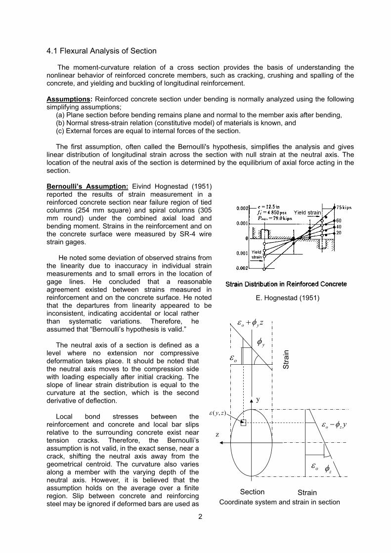
2

4.1 Flexural Analysis of Section

The moment-curvature relation of a cross section provides the basis of understanding the nonlinear behavior of reinforced concrete members, such as cracking, crushing and spalling of the concrete, and yielding and buckling of longitudinal reinforcement. Assumptions: Reinforced concrete section under bending is normally analyzed using the following simplifying assumptions;

(a) Plane section before bending remains plane and normal to the member axis after bending, (b) Normal stress-strain relation (constitutive model) of materials is known, and (c) External forces are equal to internal forces of the section. The first assumption, often called the Bernoulli's hypothesis, simplifies the analysis and gives

linear distribution of longitudinal strain across the section with null strain at the neutral axis. The location of the neutral axis of the section is determined by the equilibrium of axial force acting in the section.

Bernoulli’s Assumption: Eivind Hognestad (1951) reported the results of strain measurement in a reinforced concrete section near failure region of tied columns (254 mm square) and spiral columns (305 mm round) under the combined axial load and bending moment. Strains in the reinforcement and on the concrete surface were measured by SR-4 wire strain gages.

He noted some deviation of observed strains from the linearity due to inaccuracy in individual strain measurements and to small errors in the location of gage lines. He concluded that a reasonable agreement existed between strains measured in reinforcement and on the concrete surface. He noted that the departures from linearity appeared to be inconsistent, indicating accidental or local rather than systematic variations. Therefore, he assumed that “Bernoulli’s hypothesis is valid.”

The neutral axis of a section is defined as a

level where no extension nor compressive deformation takes place. It should be noted that the neutral axis moves to the compression side with loading especially after initial cracking. The slope of linear strain distribution is equal to the curvature at the section, which is the second derivative of deflection.

Local bond stresses between the

reinforcement and concrete and local bar slips relative to the surrounding concrete exist near tension cracks. Therefore, the Bernoulli’s assumption is not valid, in the exact sense, near a crack, shifting the neutral axis away from the geometrical centroid. The curvature also varies along a member with the varying depth of the neutral axis. However, it is believed that the assumption holds on the average over a finite region. Slip between concrete and reinforcing steel may be ignored if deformed bars are used as

E. Hognestad (1951)

o z yε φ−

y

z

oε zφ

( , )y zε

Section Strain

oεyφ

Stra

in

o y zε φ+

Coordinate system and strain in section

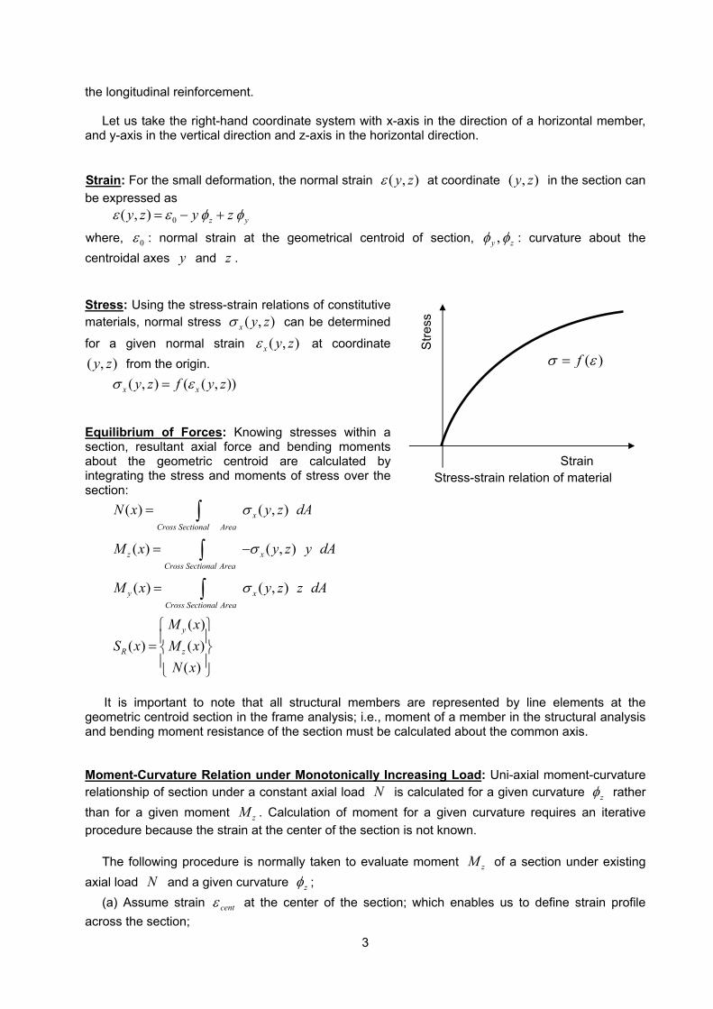
3

the longitudinal reinforcement. Let us take the right-hand coordinate system with x-axis in the direction of a horizontal member,

and y-axis in the vertical direction and z-axis in the horizontal direction.

Strain: For the small deformation, the normal strain ( , )y zε at coordinate ( , )y z in the section can be expressed as

0( , ) z yy z y zε ε φ φ= − +

where, 0ε : normal strain at the geometrical centroid of section, ,y zφ φ : curvature about the centroidal axes y and z . Stress: Using the stress-strain relations of constitutive materials, normal stress ( , )x y zσ can be determined

for a given normal strain ( , )x y zε at coordinate ( , )y z from the origin.

( , ) ( ( , ))x xy z f y zσ ε= Equilibrium of Forces: Knowing stresses within a section, resultant axial force and bending moments about the geometric centroid are calculated by integrating the stress and moments of stress over the section:

( ) ( , )

( ) ( , )

( ) ( , )

xCross Sectional Area

z xCross Sectional Area

y xCross Sectional Area

N x y z dA

M x y z y dA

M x y z z dA

σ

σ

σ

=

= −

=

∫

∫

∫

( )( ) ( )

( )

y

R z

M xS x M x

N x

=

It is important to note that all structural members are represented by line elements at the

geometric centroid section in the frame analysis; i.e., moment of a member in the structural analysis and bending moment resistance of the section must be calculated about the common axis. Moment-Curvature Relation under Monotonically Increasing Load: Uni-axial moment-curvature relationship of section under a constant axial load N is calculated for a given curvature zφ rather than for a given moment zM . Calculation of moment for a given curvature requires an iterative procedure because the strain at the center of the section is not known.

The following procedure is normally taken to evaluate moment zM of a section under existing axial load N and a given curvature zφ ;

(a) Assume strain centε at the center of the section; which enables us to define strain profile across the section;

Strain

Stre

ss

( )fσ ε=

Stress-strain relation of material

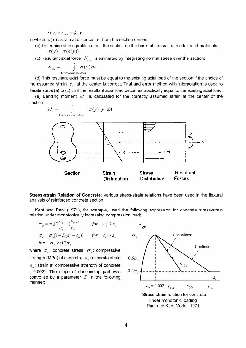
4

( ) centy yε ε φ= − in which )( yε : strain at distance y from the section center.

(b) Determine stress profile across the section on the basis of stress-strain relation of materials; ))(()( yy εσσ =

(c) Resultant axial force calN is estimated by integrating normal stress over the section;

∫=AreaSectionalCross

cal dAyN )(σ

(d) This resultant axial force must be equal to the existing axial load of the section if the choice of the assumed strain oε at the center is correct. Trial and error method with interpolation is used to iterate steps (a) to (c) until the resultant axial load becomes practically equal to the existing axial load.

(e) Bending moment zM is calculated for the correctly assumed strain at the center of the section; ( )z

Cross Sectional Area

M y y dAσ= −∫

Stress-strain Relation of Concrete: Various stress-strain relations have been used in the flexural analysis of reinforced concrete section.

Kent and Park (1971), for example, used the following expression for concrete stress-strain relation under monotonically increasing compression load;

oc

ocococ

oco

c

o

coc

butforZ

for

σσεεεεσσ

εεεε

εεσσ

2.0)](1[

])(2[ 2

≥>−−=

≤−=

where cσ : concrete stress, oσ : compressive

strength (MPa) of concrete, cε : concrete strain,

oε : strain at compressive strength of concrete (=0.002). The slope of descending part was controlled by a parameter Z in the following manner;

20ε50cε 50uε 0.002oε =

oσ

0.5 oσ

0.2 oσ50hε

cε

cσ

Confined

Unconfined

Stress-strain relation for concrete under monotonic loading

Park and Kent Model, 1971

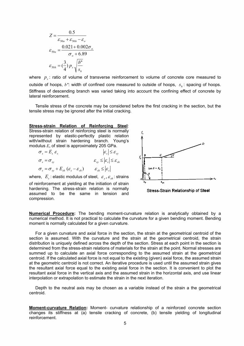
5

hsh

o

ou

ohu

sbp

Z

")43(

89.6002.0021.0

5.0

50

50

5050

=

++

=

−+=

ε

σσε

εεε

where sp : ratio of volume of transverse reinforcement to volume of concrete core measured to

outside of hoops, b": width of confined core measured to outside of hoops, hs : spacing of hoops. Stiffness of descending branch was varied taking into account the confining effect of concrete by lateral reinforcement.

Tensile stress of the concrete may be considered before the first cracking in the section, but the tensile stress may be ignored after the initial cracking. Stress-strain Relation of Reinforcing Steel: Stress-strain relation of reinforcing steel is normally represented by elastic-perfectly plastic relation with/without strain hardening branch. Young’s modulus Es of steel is approximately 205 GPa.

( )

s s s s sy

s sy sy s sh

s sy sh s sh sh s

E

E

σ ε ε ε

σ σ ε ε ε

σ σ ε ε ε ε

= ≤

= ≤ ≤

= + − ≤

where, sE : elastic modulus of steel, ,y shε ε : strains of reinforcement at yielding at the initiation of strain hardening. The stress-strain relation is normally assumed to be the same in tension and compression. Numerical Procedure: The bending moment-curvature relation is analytically obtained by a numerical method. It is not practical to calculate the curvature for a given bending moment. Bending moment is normally calculated for a given curvature.

For a given curvature and axial force in the section, the strain at the geometrical centroid of the section is assumed. With the curvature and the strain at the geometrical centroid, the strain distribution is uniquely defined across the depth of the section. Stress at each point in the section is determined from the stress-strain relations of materials for the strain at the point. Normal stresses are summed up to calculate an axial force corresponding to the assumed strain at the geometrical centroid. If the calculated axial force is not equal to the existing (given) axial force, the assumed strain at the geometric centroid is not correct. An iterative procedure is used until the assumed strain gives the resultant axial force equal to the existing axial force in the section. It is convenient to plot the resultant axial force in the vertical axis and the assumed strain in the horizontal axis, and use linear interpolation or extrapolation to estimate the strain in the next iteration.

Depth to the neutral axis may be chosen as a variable instead of the strain a the geometrical centroid. Moment-curvature Relation: Moment- curvature relationship of a reinforced concrete section changes its stiffness at (a) tensile cracking of concrete, (b) tensile yielding of longitudinal reinforcement.

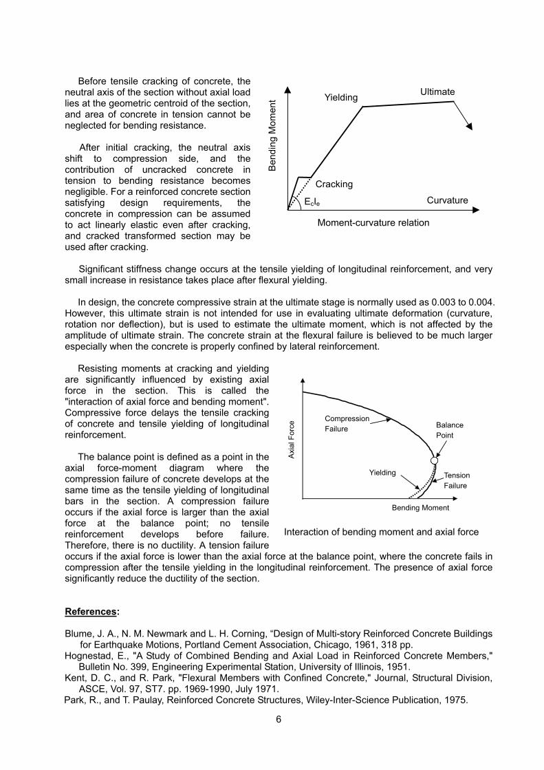
6

Before tensile cracking of concrete, the

neutral axis of the section without axial load lies at the geometric centroid of the section, and area of concrete in tension cannot be neglected for bending resistance.

After initial cracking, the neutral axis shift to compression side, and the contribution of uncracked concrete in tension to bending resistance becomes negligible. For a reinforced concrete section satisfying design requirements, the concrete in compression can be assumed to act linearly elastic even after cracking, and cracked transformed section may be used after cracking.

Significant stiffness change occurs at the tensile yielding of longitudinal reinforcement, and very

small increase in resistance takes place after flexural yielding.

In design, the concrete compressive strain at the ultimate stage is normally used as 0.003 to 0.004. However, this ultimate strain is not intended for use in evaluating ultimate deformation (curvature, rotation nor deflection), but is used to estimate the ultimate moment, which is not affected by the amplitude of ultimate strain. The concrete strain at the flexural failure is believed to be much larger especially when the concrete is properly confined by lateral reinforcement.

Resisting moments at cracking and yielding

are significantly influenced by existing axial force in the section. This is called the "interaction of axial force and bending moment". Compressive force delays the tensile cracking of concrete and tensile yielding of longitudinal reinforcement.

The balance point is defined as a point in the axial force-moment diagram where the compression failure of concrete develops at the same time as the tensile yielding of longitudinal bars in the section. A compression failure occurs if the axial force is larger than the axial force at the balance point; no tensile reinforcement develops before failure. Therefore, there is no ductility. A tension failure occurs if the axial force is lower than the axial force at the balance point, where the concrete fails in compression after the tensile yielding in the longitudinal reinforcement. The presence of axial force significantly reduce the ductility of the section. References: Blume, J. A., N. M. Newmark and L. H. Corning, “Design of Multi-story Reinforced Concrete Buildings

for Earthquake Motions, Portland Cement Association, Chicago, 1961, 318 pp. Hognestad, E., "A Study of Combined Bending and Axial Load in Reinforced Concrete Members,"

Bulletin No. 399, Engineering Experimental Station, University of Illinois, 1951. Kent, D. C., and R. Park, "Flexural Members with Confined Concrete," Journal, Structural Division,

ASCE, Vol. 97, ST7. pp. 1969-1990, July 1971. Park, R., and T. Paulay, Reinforced Concrete Structures, Wiley-Inter-Science Publication, 1975.

Yielding

Cracking

Ultimate

Curvature

Ben

ding

Mom

ent

EcIe

Moment-curvature relation

Bending Moment

Axi

al F

orce

Compression Failure

TensionFailure

Yielding

Balance Point

Interaction of bending moment and axial force

7

Pfrang, E. O., C. P. Siess and M. A. Sozen, “Load-Moment-Curvature Characteristics of Reinforced Concrete Cross Sections,“ Journal, American concrete Institute, Vol. 61, No. 7, July 1964, pp. 763 - 778.

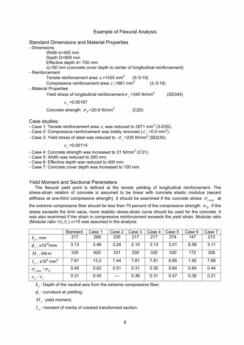
8

Example of Flexural Analysis Standard Dimensions and Material Properties - Dimensions

Width b=400 mm Depth D=800 mm Effective depth d= 750 mm dc=50 mm (concrete cover depth to center of longitudinal reinforcement)

- Reinforcement Tensile reinforcement area As=1435 mm2 (5-Ｄ19)

Compressive reinforcement area A’s=861 mm2 (3-Ｄ19) - Material Properties

Yield stress of longitudinal reinforcement yσ =345 N/mm2 (SD345)

yε =0.00167

Concrete strength Bσ =20.6 N/mm2 (C20) Case studies: - Case 1: Tensile reinforcement area As was reduced to 2871 mm2 (3-D35). - Case 2: Compressive reinforcement was totally removed (A’s =0.0 mm2). - Case 3: Yield stress of steel was reduced to yσ =235 N/mm2 (SD235).

yε =0.00114 - Case 4: Concrete strength was increased to 31 N/mm2 (C31). - Case 5: Width was reduced to 200 mm. - Case 6: Effective depth was reduced to 400 mm. - Case 7: Concrete cover depth was increased to 100 mm. Yield Moment and Sectional Parameters

The flexural yield point is defined at the tensile yielding of longitudinal reinforcement. The stress-strain relation of concrete is assumed to be linear with concrete elastic modulus (secant stiffness at one-third compressive strength). It should be examined if the concrete stress maxcσ at

the extreme compressive fiber should be less than 70 percent of the compressive strength Bσ . If the stress exceeds the limit value, more realistic stress-strain curve should be used for the concrete. It was also examined if the strain in compressive reinforcement exceeds the yield strain. Modular ratio (Modular ratio =Es/Ec) n=15 was assumed in the analysis.

Standard Case 1 Case 2 Case 3 Case 4 Case 5 Case 6 Case 7

dk , mm 217 268 235 217 217 274 147 213

yφ , x10-6/mm 3.13 3.46 3.24 2.15 3.13 3.51 6.58 3.11

yM , kN-m 335 625 331 230 335 330 172 326

crI , x105 mm4 7.81 13.2 7.44 7.81 7.81 6.85 1.92 7.66

max /c Bσ σ 0.45 0.62 0.51 0.31 0.30 0.64 0.64 0.44

/sc yε ε 0.31 0.45 --- 0.36 0.31 0.47 0.38 0.21

dk : Depth of the neutral axis from the extreme compressive fiber;

yφ : curvature at yielding;

yM : yield moment;

crI : moment of inertia of cracked transformed section.

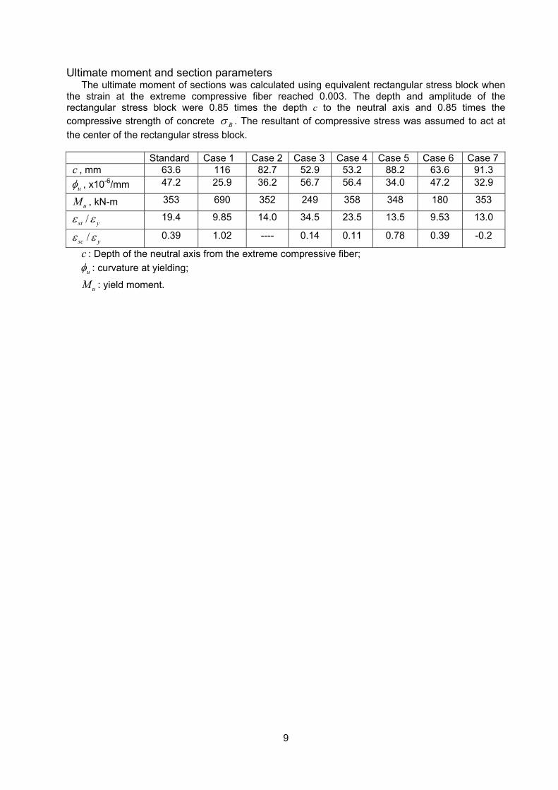
9

Ultimate moment and section parameters The ultimate moment of sections was calculated using equivalent rectangular stress block when

the strain at the extreme compressive fiber reached 0.003. The depth and amplitude of the rectangular stress block were 0.85 times the depth c to the neutral axis and 0.85 times the compressive strength of concrete Bσ . The resultant of compressive stress was assumed to act at the center of the rectangular stress block.

Standard Case 1 Case 2 Case 3 Case 4 Case 5 Case 6 Case 7c , mm 63.6 116 82.7 52.9 53.2 88.2 63.6 91.3

uφ , x10-6/mm 47.2 25.9 36.2 56.7 56.4 34.0 47.2 32.9

uM , kN-m 353 690 352 249 358 348 180 353

/st yε ε 19.4 9.85 14.0 34.5 23.5 13.5 9.53 13.0

/sc yε ε 0.39 1.02 ---- 0.14 0.11 0.78 0.39 -0.2

c : Depth of the neutral axis from the extreme compressive fiber;

uφ : curvature at yielding;

uM : yield moment.

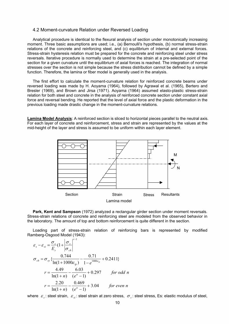
10

4.2 Moment-curvature Relation under Reversed Loading

Analytical procedure is identical to the flexural analysis of section under monotonically increasing moment. Three basic assumptions are used; i.e., (a) Bernoulli's hypothesis, (b) normal stress-strain relations of the concrete and reinforcing steel, and (c) equilibrium of internal and external forces. Stress-strain hysteresis relation must be prepared for the concrete and reinforcing steel under stress reversals. Iterative procedure is normally used to determine the strain at a pre-selected point of the section for a given curvature until the equilibrium of axial forces is reached. The integration of normal stresses over the section is not simple because the stress distribution cannot be defined by a simple function. Therefore, the lamina or fiber model is generally used in the analysis.

The first effort to calculate the moment-curvature relation for reinforced concrete beams under

reversed loading was made by H. Aoyama (1964), followed by Agrawal et al. (1965), Bertero and Bresler (1969), and Brown and Jirsa (1971). Aoyama (1964) assumed elasto-plastic stress-strain relation for both steel and concrete in the analysis of reinforced concrete section under constant axial force and reversal bending. He reported that the level of axial force and the plastic deformation in the previous loading made drastic change in the moment-curvature relations.

Lamina Model Analysis: A reinforced section is sliced to horizontal pieces parallel to the neutral axis. For each layer of concrete and reinforcement, stress and strain are represented by the values at the mid-height of the layer and stress is assumed to be uniform within each layer element.

Park, Kent and Sampson (1972) analyzed a rectangular girder section under moment reversals.

Stress-strain relations of concrete and reinforcing steel are modeled from the observed behavior in the laboratory. The amount of top and bottom reinforcement is quite different in the section.

Loading part of stress-strain relation of reinforcing bars is represented by modified

Ramberg-Osgood Model (1943):

}2411.01

71.0)10001ln(

744.0{

1(

1000

1

+−

−+

=

+=−−

ipe

E

ipsych

r

ch

s

s

ssis

εεσσ

σσσεε

nevenforen

r

noddforen

r

n

n

04.3)1(

469.0)1ln(

20.2

297.0)1(

03.6)1ln(

49.4

+−

−+

=

+−

−+

=

where sε : steel strain, siε : steel strain at zero stress, sσ : steel stress, Es: elastic modulus of steel,

StrainSection Stress Resultants

M

N

Lamina model

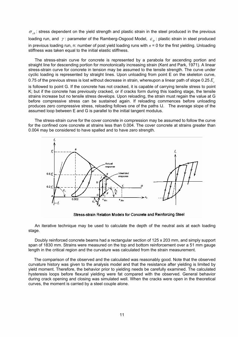
11

chσ : stress dependent on the yield strength and plastic strain in the steel produced in the previous

loading run, and γ : parameter of the Ramberg-Osgood Model, ipε : plastic strain in steel produced in previous loading run, n: number of post yield loading runs with n = 0 for the first yielding. Unloading stiffness was taken equal to the initial elastic stiffness.

The stress-strain curve for concrete is represented by a parabola for ascending portion and straight line for descending portion for monotonically increasing strain (Kent and Park, 1971). A linear stress-strain curve for concrete in tension may be assumed to the tensile strength. The curve under cyclic loading is represented by straight lines. Upon unloading from point E on the skeleton curve, 0.75 of the previous stress is lost without decrease in strain, whereupon a linear path of slope 0.25 cE is followed to point G. If the concrete has not cracked, it is capable of carrying tensile stress to point K; but if the concrete has previously cracked, or if cracks form during this loading stage, the tensile strains increase but no tensile stress develops. Upon reloading, the strain must regain the value at G before compressive stress can be sustained again. If reloading commences before unloading produces zero compressive stress, reloading follows one of the paths IJ. The average slope of the assumed loop between E and G is parallel to the initial tangent modulus.

The stress-strain curve for the cover concrete in compression may be assumed to follow the curve

for the confined core concrete at strains less than 0.004. The cover concrete at strains greater than 0.004 may be considered to have spalled and to have zero strength.

An iterative technique may be used to calculate the depth of the neutral axis at each loading stage.

Doubly reinforced concrete beams had a rectangular section of 125 x 203 mm, and simply support span of 1830 mm. Strains were measured on the top and bottom reinforcement over a 51 mm gauge length in the critical region and the curvature was calculated from the strain measurement.

The comparison of the observed and the calculated was reasonably good. Note that the observed

curvature history was given to the analysis model and that the resistance after yielding is limited by yield moment. Therefore, the behavior prior to yielding needs be carefully examined. The calculated hysteresis loops before flexural yielding were fat compared with the observed. General behavior during crack opening and closing was simulated well. When the cracks were open in the theoretical curves, the moment is carried by a steel couple alone.

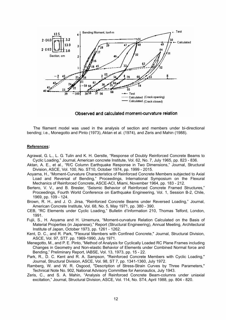
12

The filament model was used in the analysis of section and members under bi-directional

bending; i.e., Monegotto and Pinto (1973), Aktan et al. (1974), and Zeris and Mahin (1988). References: Agrawal, G. L., L. G. Tulin and K. H. Gerstle, “Response of Doubly Reinforced Concrete Beams to

Cyclic Loading,” Journal, American concrete Institute, Vol. 62, No. 7, July 1965, pp. 823 - 836. Aktan, A. E., et al., “R/C Column Earthquake Response in Two Dimensions,” Journal, Structural

Division, ASCE, Vol. 100, No. ST10, October 1974, pp. 1999 - 2015. Aoyama, H., “Moment-Curvature Characteristics of Reinforced Concrete Members subjected to Axial

Load and Reversal of Bending,” Proceedings, International Symposium on the Flexural Mechanics of Reinforced Concrete, ASCE-ACI, Miami, November 1964, pp. 183 - 212.

Bertero, V. V., and B. Bresler, “Seismic Behavior of Reinforced Concrete Framed Structures,” Proceedings, Fourth World Conference on Earthquake Engineering, Vol. 1, Session B-2, Chile, 1969, pp. 109 - 124.

Brown, R. H., and J. O. Jirsa, “Reinforced Concrete Beams under Reversed Loading,” Journal, American Concrete Institute, Vol. 68, No. 5, May 1971, pp. 380 - 390.

CEB, “RC Elements under Cyclic Loading,” Bulletin d’Information 210, Thomas Telford, London, 1991.

Fujii, S., H. Aoyama and H. Umemura, “Moment-curvature Relation Calculated on the Basis of Material Properties (in Japanese),” Report (Structural Engineering), Annual Meeting, Architectural Institute of Japan, October 1973, pp. 1261 - 1262.

Kent, D. C., and R. Park, "Flexural Members with Confined Concrete," Journal, Structural Division, ASCE, Vol. 97, ST7. pp. 1969-1990, July 1971.

Menegotto, M., and P. E. Pinto, “Method of Analysis for Cyclically Loaded RC Plane Frames including Changes in Geometry and Non-elastic Behavior of Elements under Combined Normal force and Bending,” Preliminary Report, IABSE, Vol. 13, 1973, pp. 15 - 22.

Park, R., D. C. Kent and R. A. Sampson, "Reinforced Concrete Members with Cyclic Loading," Journal, Structural Division, ASCE, Vol. 98, ST 7, pp. 1341-1360, July 1972.

Ramberg, W. and W. R. Osgood, "Description of Stress-Strain Curves by Three Parameters," Technical Note No. 902, National Advisory Committee for Aeronautics, July 1943.

Zeris, C., and S. A. Mahin, “Analysis of Reinforced Concrete Beam-columns under uniaxial excitation,” Journal, Structural Division, ASCE, Vol. 114, No. ST4, April 1988, pp. 804 - 820.

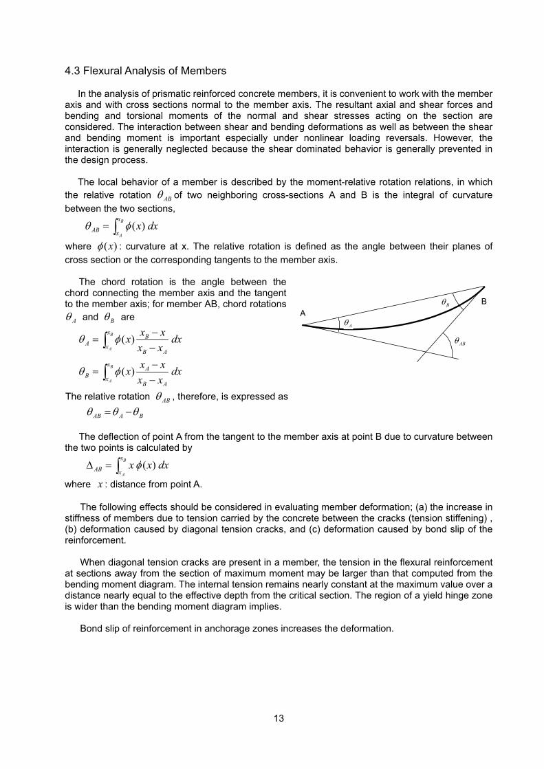
13

4.3 Flexural Analysis of Members In the analysis of prismatic reinforced concrete members, it is convenient to work with the member

axis and with cross sections normal to the member axis. The resultant axial and shear forces and bending and torsional moments of the normal and shear stresses acting on the section are considered. The interaction between shear and bending deformations as well as between the shear and bending moment is important especially under nonlinear loading reversals. However, the interaction is generally neglected because the shear dominated behavior is generally prevented in the design process.

The local behavior of a member is described by the moment-relative rotation relations, in which

the relative rotation ABθ of two neighboring cross-sections A and B is the integral of curvature between the two sections,

( )B

A

x

AB xx dxθ φ= ∫

where ( )xφ : curvature at x. The relative rotation is defined as the angle between their planes of cross section or the corresponding tangents to the member axis.

The chord rotation is the angle between the chord connecting the member axis and the tangent to the member axis; for member AB, chord rotations

Aθ and Bθ are

( )

( )

B

A

B

A

x BA x

B A

x AB x

B A

x xx dxx xx xx dxx x

θ φ

θ φ

−=

−−

=−

∫

∫

The relative rotation ABθ , therefore, is expressed as

AB A Bθ θ θ= −

The deflection of point A from the tangent to the member axis at point B due to curvature between the two points is calculated by

( )B

A

x

AB xx x dxφ∆ = ∫

where x : distance from point A.

The following effects should be considered in evaluating member deformation; (a) the increase in stiffness of members due to tension carried by the concrete between the cracks (tension stiffening) , (b) deformation caused by diagonal tension cracks, and (c) deformation caused by bond slip of the reinforcement.

When diagonal tension cracks are present in a member, the tension in the flexural reinforcement

at sections away from the section of maximum moment may be larger than that computed from the bending moment diagram. The internal tension remains nearly constant at the maximum value over a distance nearly equal to the effective depth from the critical section. The region of a yield hinge zone is wider than the bending moment diagram implies.

Bond slip of reinforcement in anchorage zones increases the deformation.

Aθ

Bθ

ABθ

AB

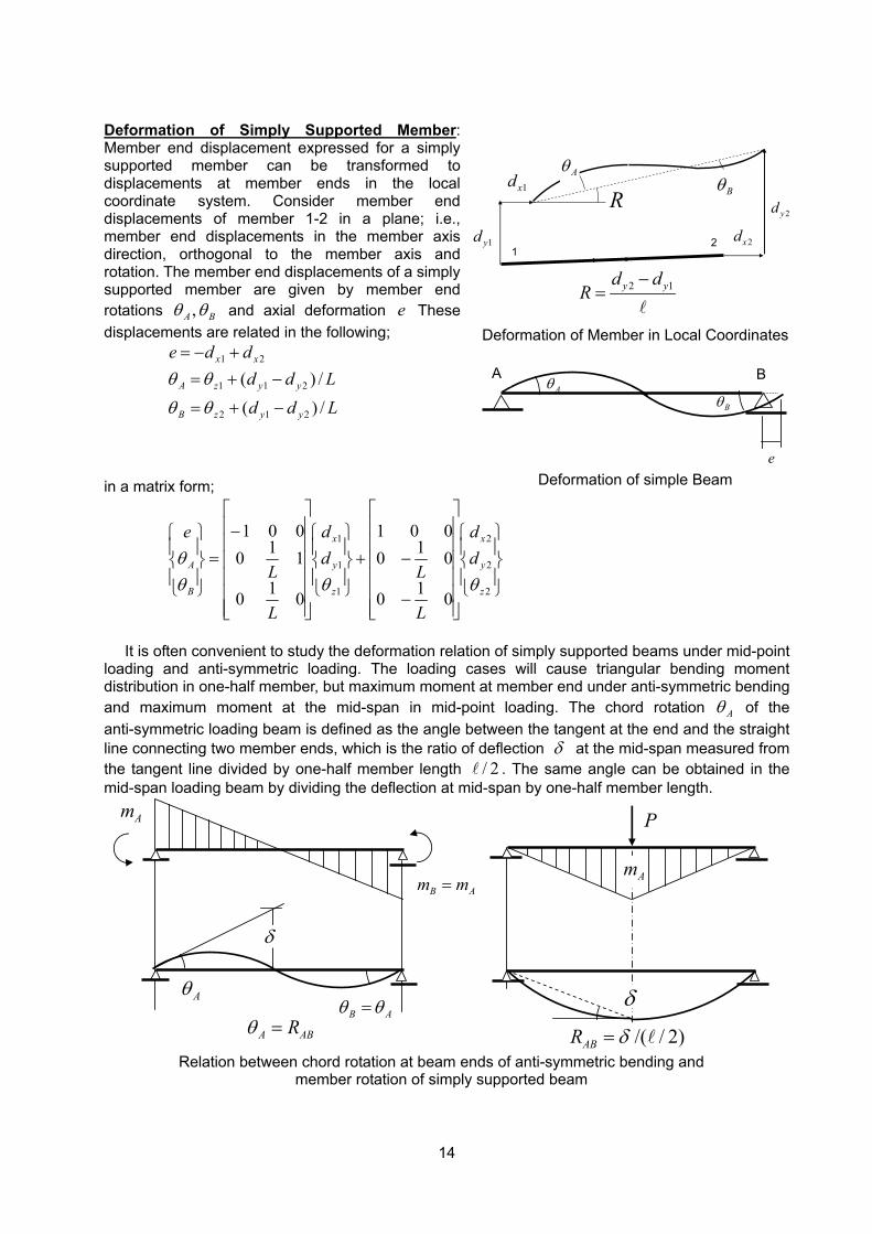
14

Deformation of Simply Supported Member: Member end displacement expressed for a simply supported member can be transformed to displacements at member ends in the local coordinate system. Consider member end displacements of member 1-2 in a plane; i.e., member end displacements in the member axis direction, orthogonal to the member axis and rotation. The member end displacements of a simply supported member are given by member end rotations ,A Bθ θ and axial deformation e These displacements are related in the following;

LddLdd

dde

yyzB

yyzA

xx

/)(/)(

212

211

21

−+=

−+=+−=

θθ

θθ

in a matrix form;

−

−+

−

=

2

2

2

1

1

1

010

010001

010

110001

z

y

x

z

y

x

B

A dd

L

Ldd

L

L

e

θθθθ

It is often convenient to study the deformation relation of simply supported beams under mid-point

loading and anti-symmetric loading. The loading cases will cause triangular bending moment distribution in one-half member, but maximum moment at member end under anti-symmetric bending and maximum moment at the mid-span in mid-point loading. The chord rotation Aθ of the anti-symmetric loading beam is defined as the angle between the tangent at the end and the straight line connecting two member ends, which is the ratio of deflection δ at the mid-span measured from the tangent line divided by one-half member length / 2l . The same angle can be obtained in the mid-span loading beam by dividing the deflection at mid-span by one-half member length.

R

AθBθ

1 2 1yd

1xd

2xd2yd

2 1y yd dR

−=

l

Deformation of Member in Local Coordinates

BθAθ

A B

e Deformation of simple Beam

Am

B Am m=

δ

Aθ B Aθ θ=

A ABRθ = /( / 2)ABR δ= l

δ

Am

P

Relation between chord rotation at beam ends of anti-symmetric bending and member rotation of simply supported beam

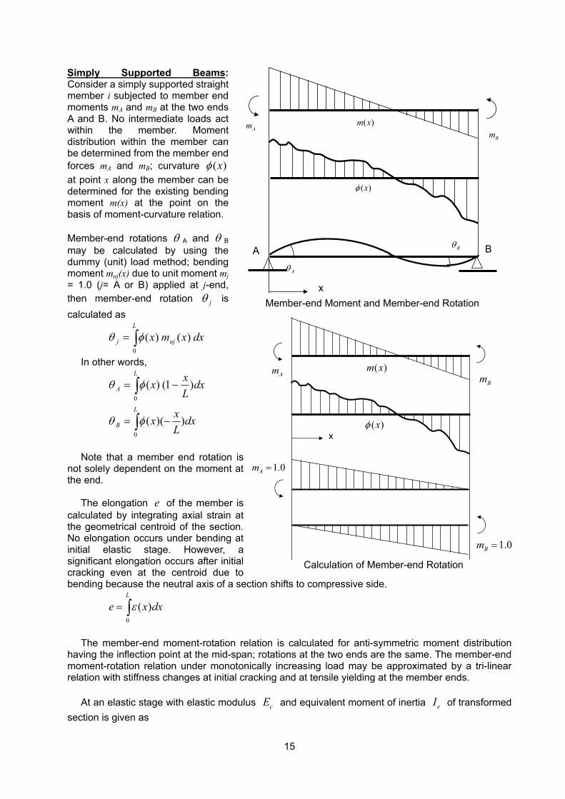
15

Simply Supported Beams: Consider a simply supported straight member i subjected to member end moments mA and mB at the two ends A and B. No intermediate loads act within the member. Moment distribution within the member can be determined from the member end forces mA and mB; curvature )(xφ at point x along the member can be determined for the existing bending moment m(x) at the point on the basis of moment-curvature relation. Member-end rotations θ A and θ B may be calculated by using the dummy (unit) load method; bending moment muj(x) due to unit moment mj = 1.0 (j= A or B) applied at j-end, then member-end rotation jθ is calculated as

∫=L

ujj dxxmx0

)()(φθ

In other words,

dxLxx

dxLxx

L

B

L

A

)()(

)1()(

0

0

−=

−=

∫

∫

φθ

φθ

Note that a member end rotation is

not solely dependent on the moment at the end.

The elongation e of the member is

calculated by integrating axial strain at the geometrical centroid of the section. No elongation occurs under bending at initial elastic stage. However, a significant elongation occurs after initial cracking even at the centroid due to bending because the neutral axis of a section shifts to compressive side.

∫=L

dxxe0

)(ε

The member-end moment-rotation relation is calculated for anti-symmetric moment distribution

having the inflection point at the mid-span; rotations at the two ends are the same. The member-end moment-rotation relation under monotonically increasing load may be approximated by a tri-linear relation with stiffness changes at initial cracking and at tensile yielding at the member ends.

At an elastic stage with elastic modulus cE and equivalent moment of inertia eI of transformed

section is given as

x

A BBθ

Aθ

( )m x

( )xφ

AmBm

Member-end Moment and Member-end Rotation

( )m x

( )xφ

AmBm

x

1.0Am =

1.0Bm =

Calculation of Member-end Rotation

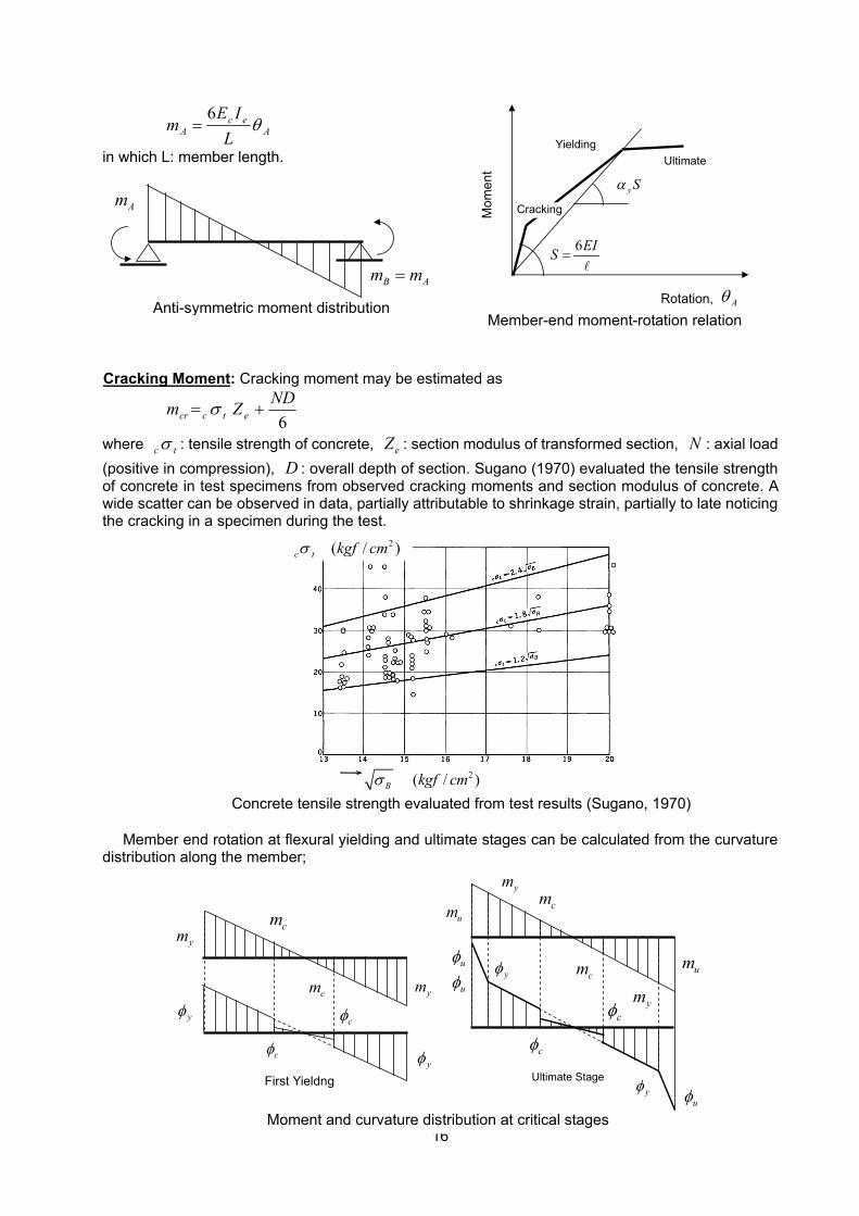
16

Aec

A LIE

m θ6

=

in which L: member length.

Cracking Moment: Cracking moment may be estimated as

6NDZm etccr += σ

where tcσ : tensile strength of concrete, eZ : section modulus of transformed section, N : axial load (positive in compression), D : overall depth of section. Sugano (1970) evaluated the tensile strength of concrete in test specimens from observed cracking moments and section modulus of concrete. A wide scatter can be observed in data, partially attributable to shrinkage strain, partially to late noticing the cracking in a specimen during the test.

Member end rotation at flexural yielding and ultimate stages can be calculated from the curvature

distribution along the member;

Rotation, Aθ

Mom

ent

Cracking

Yielding Ultimate

6EIS =l

ySα

Member-end moment-rotation relation

Am

B Am m=

Anti-symmetric moment distribution

2( / )B kgf cmσ

2( / )c t kgf cmσ

Concrete tensile strength evaluated from test results (Sugano, 1970)

First Yieldng Ultimate Stage

ym

ym

yφ

yφcφ

cφ

um

um

ym

ym

cm

cm

cm

cmuφ

uφ

uφ

yφ

yφ

cφ

cφ

Moment and curvature distribution at critical stages

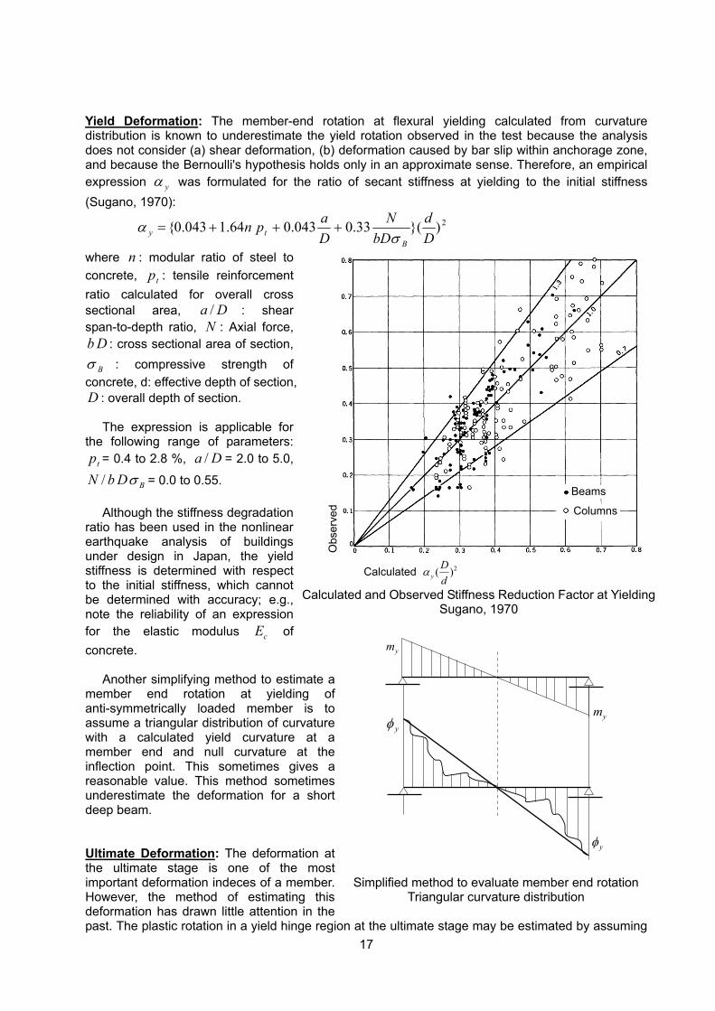
17

Yield Deformation: The member-end rotation at flexural yielding calculated from curvature distribution is known to underestimate the yield rotation observed in the test because the analysis does not consider (a) shear deformation, (b) deformation caused by bar slip within anchorage zone, and because the Bernoulli's hypothesis holds only in an approximate sense. Therefore, an empirical expression yα was formulated for the ratio of secant stiffness at yielding to the initial stiffness (Sugano, 1970):

2)}(33.0043.064.1043.0{Dd

bDN

Dapn

Bty σ

α +++=

where n : modular ratio of steel to concrete, tp : tensile reinforcement ratio calculated for overall cross sectional area, /a D : shear span-to-depth ratio, N : Axial force, b D : cross sectional area of section,

Bσ : compressive strength of concrete, d: effective depth of section, D : overall depth of section.

The expression is applicable for the following range of parameters:

tp = 0.4 to 2.8 %, /a D = 2.0 to 5.0,

/ BN b Dσ = 0.0 to 0.55.

Although the stiffness degradation ratio has been used in the nonlinear earthquake analysis of buildings under design in Japan, the yield stiffness is determined with respect to the initial stiffness, which cannot be determined with accuracy; e.g., note the reliability of an expression for the elastic modulus cE of concrete.

Another simplifying method to estimate a

member end rotation at yielding of anti-symmetrically loaded member is to assume a triangular distribution of curvature with a calculated yield curvature at a member end and null curvature at the inflection point. This sometimes gives a reasonable value. This method sometimes underestimate the deformation for a short deep beam. Ultimate Deformation: The deformation at the ultimate stage is one of the most important deformation indeces of a member. However, the method of estimating this deformation has drawn little attention in the past. The plastic rotation in a yield hinge region at the ultimate stage may be estimated by assuming

Beams

Columns

Calculated 2( )yDd

α

Obs

erve

d

Calculated and Observed Stiffness Reduction Factor at YieldingSugano, 1970

ym

ym

yφ

yφ

Simplified method to evaluate member end rotation

Triangular curvature distribution

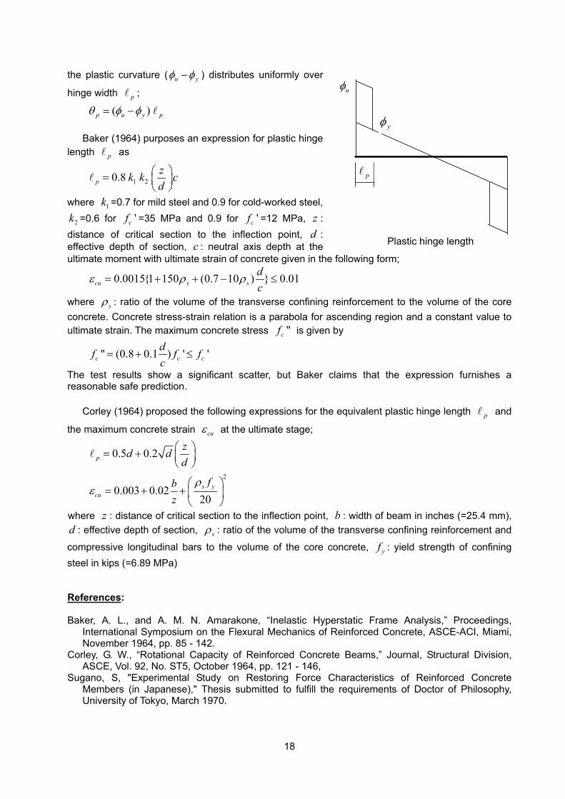
18

the plastic curvature ( u yφ φ− ) distributes uniformly over

hinge width pl ;

( )p u y pθ φ φ= − l Baker (1964) purposes an expression for plastic hinge

length pl as

1 20.8pzk k cd

=

l

where 1k =0.7 for mild steel and 0.9 for cold-worked steel,

2k =0.6 for 'cf =35 MPa and 0.9 for 'cf =12 MPa, z : distance of critical section to the inflection point, d : effective depth of section, c : neutral axis depth at the ultimate moment with ultimate strain of concrete given in the following form;

0.0015{1 150 (0.7 10 ) } 0.01cu s sdc

ε ρ ρ= + + − ≤

where sρ : ratio of the volume of the transverse confining reinforcement to the volume of the core concrete. Concrete stress-strain relation is a parabola for ascending region and a constant value to ultimate strain. The maximum concrete stress "cf is given by

" (0.8 0.1 ) ' 'c c cdf f fc

= + ≤

The test results show a significant scatter, but Baker claims that the expression furnishes a reasonable safe prediction.

Corley (1964) proposed the following expressions for the equivalent plastic hinge length pl and

the maximum concrete strain cuε at the ultimate stage;

2

0.5 0.2

0.003 0.0220

p

s ycu

zd dd

fbz

ρε

= +

= + +

l

where z : distance of critical section to the inflection point, b : width of beam in inches (=25.4 mm), d : effective depth of section, sρ : ratio of the volume of the transverse confining reinforcement and

compressive longitudinal bars to the volume of the core concrete, yf : yield strength of confining steel in kips (=6.89 MPa) References: Baker, A. L., and A. M. N. Amarakone, “Inelastic Hyperstatic Frame Analysis,” Proceedings,

International Symposium on the Flexural Mechanics of Reinforced Concrete, ASCE-ACI, Miami, November 1964, pp. 85 - 142.

Corley, G. W., “Rotational Capacity of Reinforced Concrete Beams,” Journal, Structural Division, ASCE, Vol. 92, No. ST5, October 1964, pp. 121 - 146,

Sugano, S, "Experimental Study on Restoring Force Characteristics of Reinforced Concrete Members (in Japanese)," Thesis submitted to fulfill the requirements of Doctor of Philosophy, University of Tokyo, March 1970.

uφ

yφ

pl

Plastic hinge length

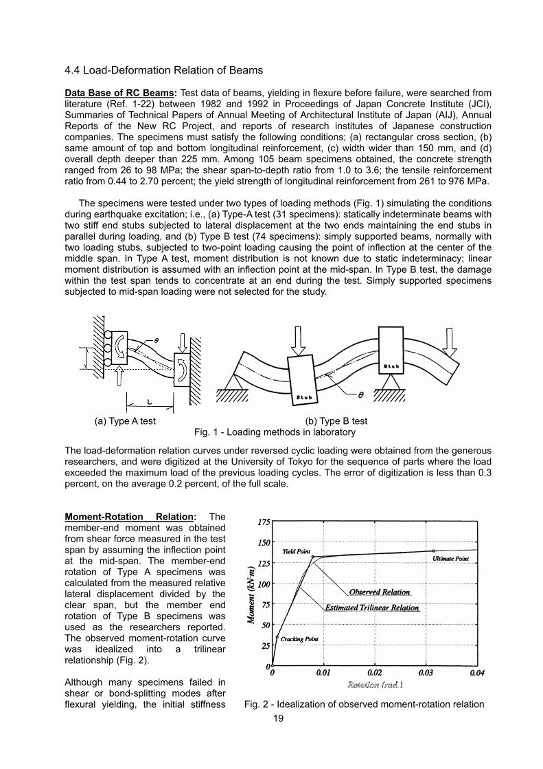
19

4.4 Load-Deformation Relation of Beams Data Base of RC Beams: Test data of beams, yielding in flexure before failure, were searched from literature (Ref. 1-22) between 1982 and 1992 in Proceedings of Japan Concrete Institute (JCI), Summaries of Technical Papers of Annual Meeting of Architectural Institute of Japan (AIJ), Annual Reports of the New RC Project, and reports of research institutes of Japanese construction companies. The specimens must satisfy the following conditions; (a) rectangular cross section, (b) same amount of top and bottom longitudinal reinforcement, (c) width wider than 150 mm, and (d) overall depth deeper than 225 mm. Among 105 beam specimens obtained, the concrete strength ranged from 26 to 98 MPa; the shear span-to-depth ratio from 1.0 to 3.6; the tensile reinforcement ratio from 0.44 to 2.70 percent; the yield strength of longitudinal reinforcement from 261 to 976 MPa.

The specimens were tested under two types of loading methods (Fig. 1) simulating the conditions during earthquake excitation; i.e., (a) Type-A test (31 specimens): statically indeterminate beams with two stiff end stubs subjected to lateral displacement at the two ends maintaining the end stubs in parallel during loading, and (b) Type B test (74 specimens): simply supported beams, normally with two loading stubs, subjected to two-point loading causing the point of inflection at the center of the middle span. In Type A test, moment distribution is not known due to static indeterminacy; linear moment distribution is assumed with an inflection point at the mid-span. In Type B test, the damage within the test span tends to concentrate at an end during the test. Simply supported specimens subjected to mid-span loading were not selected for the study.

The load-deformation relation curves under reversed cyclic loading were obtained from the generous researchers, and were digitized at the University of Tokyo for the sequence of parts where the load exceeded the maximum load of the previous loading cycles. The error of digitization is less than 0.3 percent, on the average 0.2 percent, of the full scale. Moment-Rotation Relation: The member-end moment was obtained from shear force measured in the test span by assuming the inflection point at the mid-span. The member-end rotation of Type A specimens was calculated from the measured relative lateral displacement divided by the clear span, but the member end rotation of Type B specimens was used as the researchers reported. The observed moment-rotation curve was idealized into a trilinear relationship (Fig. 2). Although many specimens failed in shear or bond-splitting modes after flexural yielding, the initial stiffness

(a) Type A test (b) Type B test Fig. 1 - Loading methods in laboratory

Fig. 2 - Idealization of observed moment-rotation relation

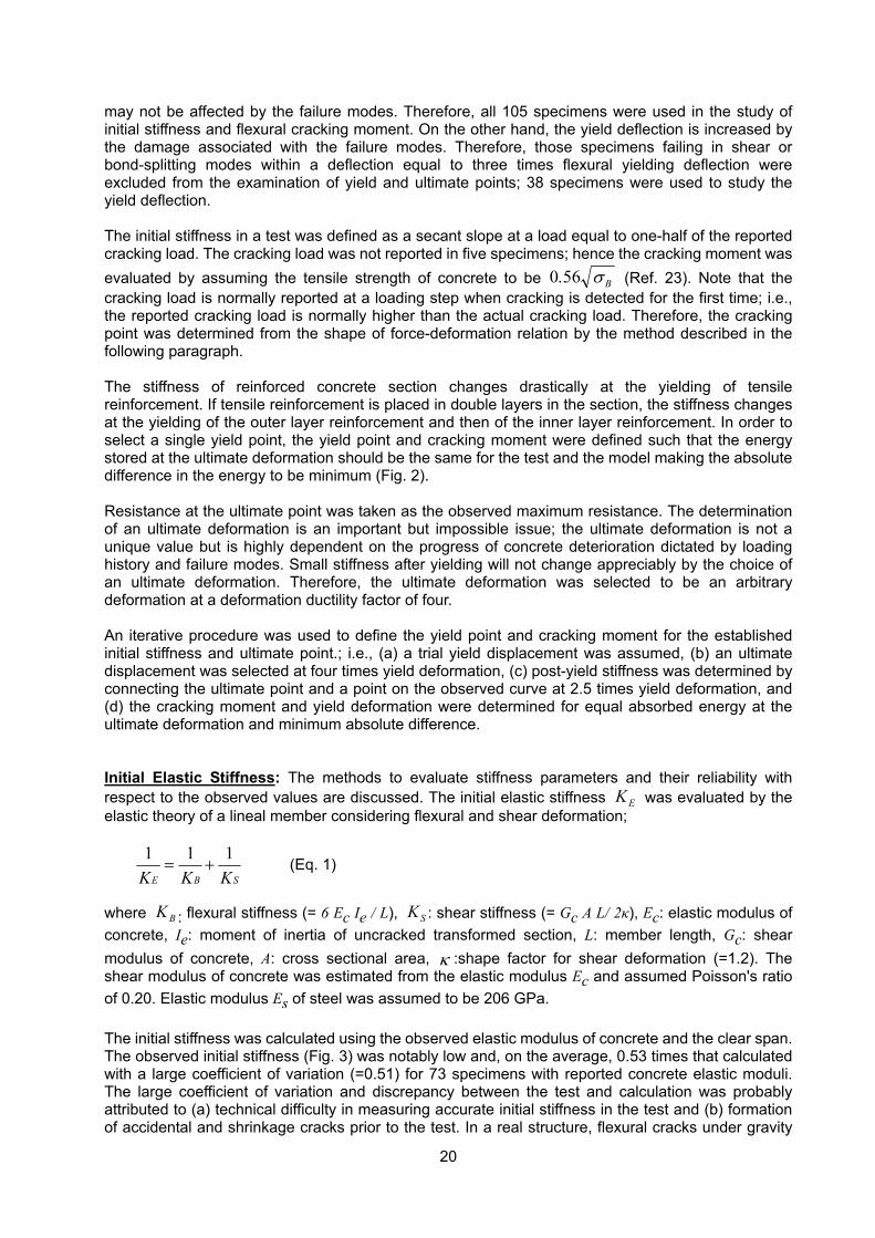
20

may not be affected by the failure modes. Therefore, all 105 specimens were used in the study of initial stiffness and flexural cracking moment. On the other hand, the yield deflection is increased by the damage associated with the failure modes. Therefore, those specimens failing in shear or bond-splitting modes within a deflection equal to three times flexural yielding deflection were excluded from the examination of yield and ultimate points; 38 specimens were used to study the yield deflection. The initial stiffness in a test was defined as a secant slope at a load equal to one-half of the reported cracking load. The cracking load was not reported in five specimens; hence the cracking moment was evaluated by assuming the tensile strength of concrete to be 0 56. σB (Ref. 23). Note that the cracking load is normally reported at a loading step when cracking is detected for the first time; i.e., the reported cracking load is normally higher than the actual cracking load. Therefore, the cracking point was determined from the shape of force-deformation relation by the method described in the following paragraph. The stiffness of reinforced concrete section changes drastically at the yielding of tensile reinforcement. If tensile reinforcement is placed in double layers in the section, the stiffness changes at the yielding of the outer layer reinforcement and then of the inner layer reinforcement. In order to select a single yield point, the yield point and cracking moment were defined such that the energy stored at the ultimate deformation should be the same for the test and the model making the absolute difference in the energy to be minimum (Fig. 2). Resistance at the ultimate point was taken as the observed maximum resistance. The determination of an ultimate deformation is an important but impossible issue; the ultimate deformation is not a unique value but is highly dependent on the progress of concrete deterioration dictated by loading history and failure modes. Small stiffness after yielding will not change appreciably by the choice of an ultimate deformation. Therefore, the ultimate deformation was selected to be an arbitrary deformation at a deformation ductility factor of four. An iterative procedure was used to define the yield point and cracking moment for the established initial stiffness and ultimate point.; i.e., (a) a trial yield displacement was assumed, (b) an ultimate displacement was selected at four times yield deformation, (c) post-yield stiffness was determined by connecting the ultimate point and a point on the observed curve at 2.5 times yield deformation, and (d) the cracking moment and yield deformation were determined for equal absorbed energy at the ultimate deformation and minimum absolute difference. Initial Elastic Stiffness: The methods to evaluate stiffness parameters and their reliability with respect to the observed values are discussed. The initial elastic stiffness KE was evaluated by the elastic theory of a lineal member considering flexural and shear deformation;

1 1 1K K KE B S

= + (Eq. 1)

where KB : flexural stiffness (= 6 Ec Ie / L), KS : shear stiffness (= Gc A L/ 2κ), Ec: elastic modulus of concrete, Ie: moment of inertia of uncracked transformed section, L: member length, Gc: shear modulus of concrete, A: cross sectional area, κ :shape factor for shear deformation (=1.2). The shear modulus of concrete was estimated from the elastic modulus Ec and assumed Poisson's ratio of 0.20. Elastic modulus Es of steel was assumed to be 206 GPa. The initial stiffness was calculated using the observed elastic modulus of concrete and the clear span. The observed initial stiffness (Fig. 3) was notably low and, on the average, 0.53 times that calculated with a large coefficient of variation (=0.51) for 73 specimens with reported concrete elastic moduli. The large coefficient of variation and discrepancy between the test and calculation was probably attributed to (a) technical difficulty in measuring accurate initial stiffness in the test and (b) formation of accidental and shrinkage cracks prior to the test. In a real structure, flexural cracks under gravity

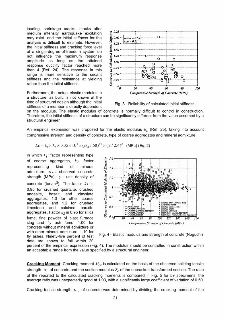
21

loading, shrinkage cracks, cracks after medium intensity earthquake excitation may exist, and the initial stiffness for the analysis is difficult to estimate. However, the initial stiffness and cracking force level of a single-degree-of-freedom system do not influence the maximum response amplitude as long as the attained response ductility factor reached more than 4 (Ref. 24). The response in this range is more sensitive to the secant stiffness and the resistance at yielding rather than the initial stiffness. Furthermore, the actual elastic modulus in a structure, as built, is not known at the time of structural design although the initial stiffness of a member is directly dependent on the modulus. The elastic modulus of concrete is normally difficult to control in construction. Therefore, the initial stiffness of a structure can be significantly different from the value assumed by a structural engineer. An empirical expression was proposed for the elastic modulus Ec (Ref. 25), taking into account compressive strength and density of concrete, type of coarse aggregates and mineral admixture;

Ec k k B= × × × × ×1 2

4 1 3 23 35 10 60 2 4. ( / ) ( / . )/σ γ (MPa) (Eq. 2) in which k1: factor representing type of coarse aggregates, k2: factor representing kind of mineral admixture, σB : observed concrete strength (MPa), γ : unit density of

concrete (ton/m3). The factor k1 is 0.95 for crushed quartzite, crushed andesite, basalt and clayslate aggregates, 1.0 for other coarse aggregates, and 1.2 for crushed limestone and calcined bauxite aggregates. Factor k2 is 0.95 for silica fume; fine powder of blast furnace slag and fly ash fume, 1.00 for concrete without mineral admixture or with other mineral admixture, 1.10 for fly ashes. Ninety-five percent of test data are shown to fall within 20 percent of the empirical expression (Fig. 4). The modulus should be controlled in construction within an acceptable range from the value specified by a structural engineer. Cracking Moment: Cracking moment Mcr is calculated on the basis of the observed splitting tensile strength σ t of concrete and the section modulus Ze of the uncracked transformed section. The ratio of the reported to the calculated cracking moments is compared in Fig. 5 for 59 specimens; the average ratio was unexpectedly good at 1.03, with a significantly large coefficient of variation of 0.50. Cracking tensile strength σcr of concrete was determined by dividing the cracking moment of the

Fig. 3 - Reliability of calculated initial stiffness

Fig. 4 - Elastic modulus and strength of concrete (Noguchi)

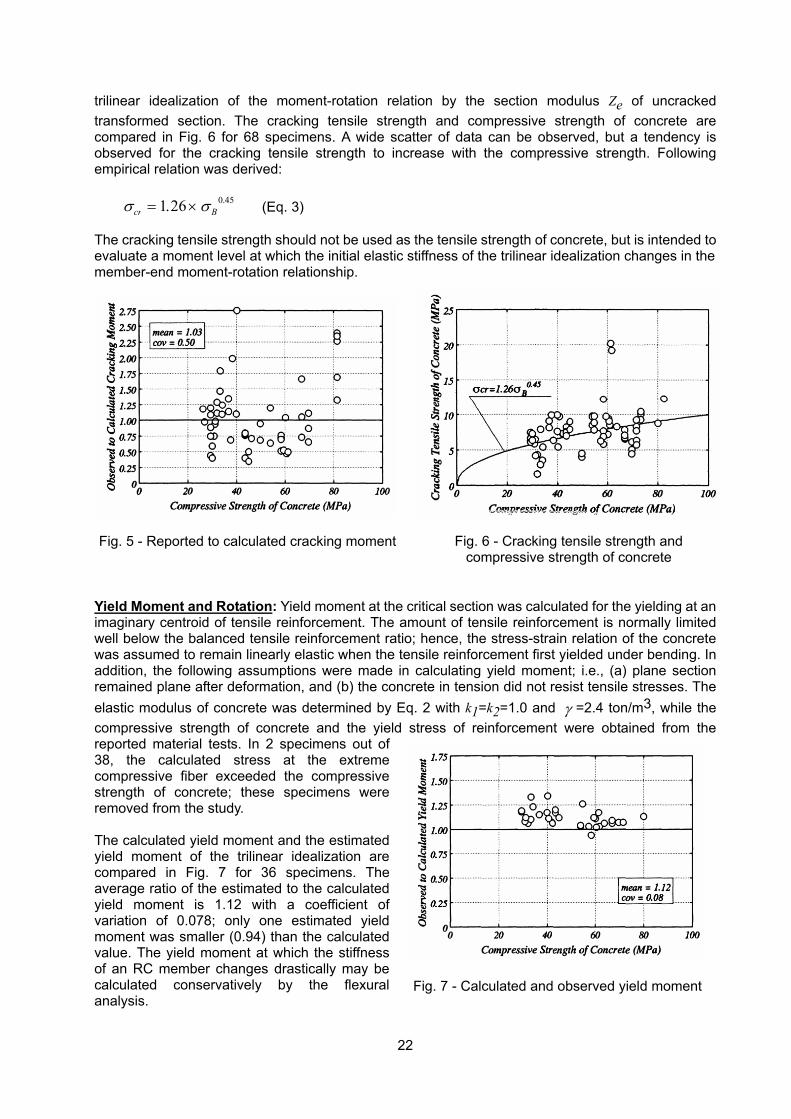
22

trilinear idealization of the moment-rotation relation by the section modulus Ze of uncracked transformed section. The cracking tensile strength and compressive strength of concrete are compared in Fig. 6 for 68 specimens. A wide scatter of data can be observed, but a tendency is observed for the cracking tensile strength to increase with the compressive strength. Following empirical relation was derived:

σ σcr B= ×1 26 0 45. . (Eq. 3) The cracking tensile strength should not be used as the tensile strength of concrete, but is intended to evaluate a moment level at which the initial elastic stiffness of the trilinear idealization changes in the member-end moment-rotation relationship.

Yield Moment and Rotation: Yield moment at the critical section was calculated for the yielding at an imaginary centroid of tensile reinforcement. The amount of tensile reinforcement is normally limited well below the balanced tensile reinforcement ratio; hence, the stress-strain relation of the concrete was assumed to remain linearly elastic when the tensile reinforcement first yielded under bending. In addition, the following assumptions were made in calculating yield moment; i.e., (a) plane section remained plane after deformation, and (b) the concrete in tension did not resist tensile stresses. The elastic modulus of concrete was determined by Eq. 2 with k1=k2=1.0 and γ =2.4 ton/m3, while the compressive strength of concrete and the yield stress of reinforcement were obtained from the reported material tests. In 2 specimens out of 38, the calculated stress at the extreme compressive fiber exceeded the compressive strength of concrete; these specimens were removed from the study. The calculated yield moment and the estimated yield moment of the trilinear idealization are compared in Fig. 7 for 36 specimens. The average ratio of the estimated to the calculated yield moment is 1.12 with a coefficient of variation of 0.078; only one estimated yield moment was smaller (0.94) than the calculated value. The yield moment at which the stiffness of an RC member changes drastically may be calculated conservatively by the flexural analysis.

Fig. 5 - Reported to calculated cracking moment

Fig. 6 - Cracking tensile strength and

compressive strength of concrete

Fig. 7 - Calculated and observed yield moment

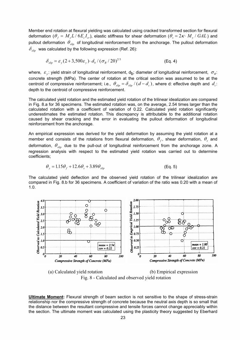
23

Member end rotation at flexural yielding was calculated using cracked transformed section for flexural deformation (θ f y c crM L E I= / 6 ), elastic stiffness for shear deformation (θ κs yM GAL= ⋅2 / ) and pullout deformation θslip of longitudinal reinforcement from the anchorage. The pullout deformation δ slip was calculated by the following expression (Ref. 26): δ ε ε σslip y y b Bd= + ⋅( , ) / ( / ) /2 3 500 20 2 3 (Eq. 4) where, ε y : yield strain of longitudinal reinforcement, db: diameter of longitudinal reinforcement, σB: concrete strength (MPa). The center of rotation at the critical section was assumed to be at the centroid of compressive reinforcement; i.e., θ δslip slip cd d= −/ ( ) , where d: effective depth and dc: depth to the centroid of compressive reinforcement. The calculated yield rotation and the estimated yield rotation of the trilinear idealization are compared in Fig. 8.a for 36 specimens. The estimated rotation was, on the average, 2.54 times larger than the calculated rotation with a coefficient of variation of 0.22. Calculated yield rotation significantly underestimates the estimated rotation. This discrepancy is attributable to the additional rotation caused by shear cracking and the error in evaluating the pullout deformation of longitudinal reinforcement from the anchorage. An empirical expression was derived for the yield deformation by assuming the yield rotation at a member end consists of the rotations from flexural deformation, θ f , shear deformation, θs and deformation, θslip due to the pull-out of longitudinal reinforcement from the anchorage zone. A regression analysis with respect to the estimated yield rotation was carried out to determine coefficients; θ θ θ θy f s slip= + +115 12 6 3 89. . . (Eq. 5) The calculated yield deflection and the observed yield rotation of the trilinear idealization are compared in Fig. 8.b for 36 specimens. A coefficient of variation of the ratio was 0.20 with a mean of 1.0.

Ultimate Moment: Flexural strength of beam section is not sensitive to the shape of stress-strain relationship nor the compressive strength of concrete because the neutral axis depth is so small that the distance between the resultant compressive and tensile forces cannot change appreciably within the section. The ultimate moment was calculated using the plasticity theory suggested by Eberhard

(a) Calculated yield rotation (b) Empirical expression Fig. 8 - Calculated and observed yield rotation

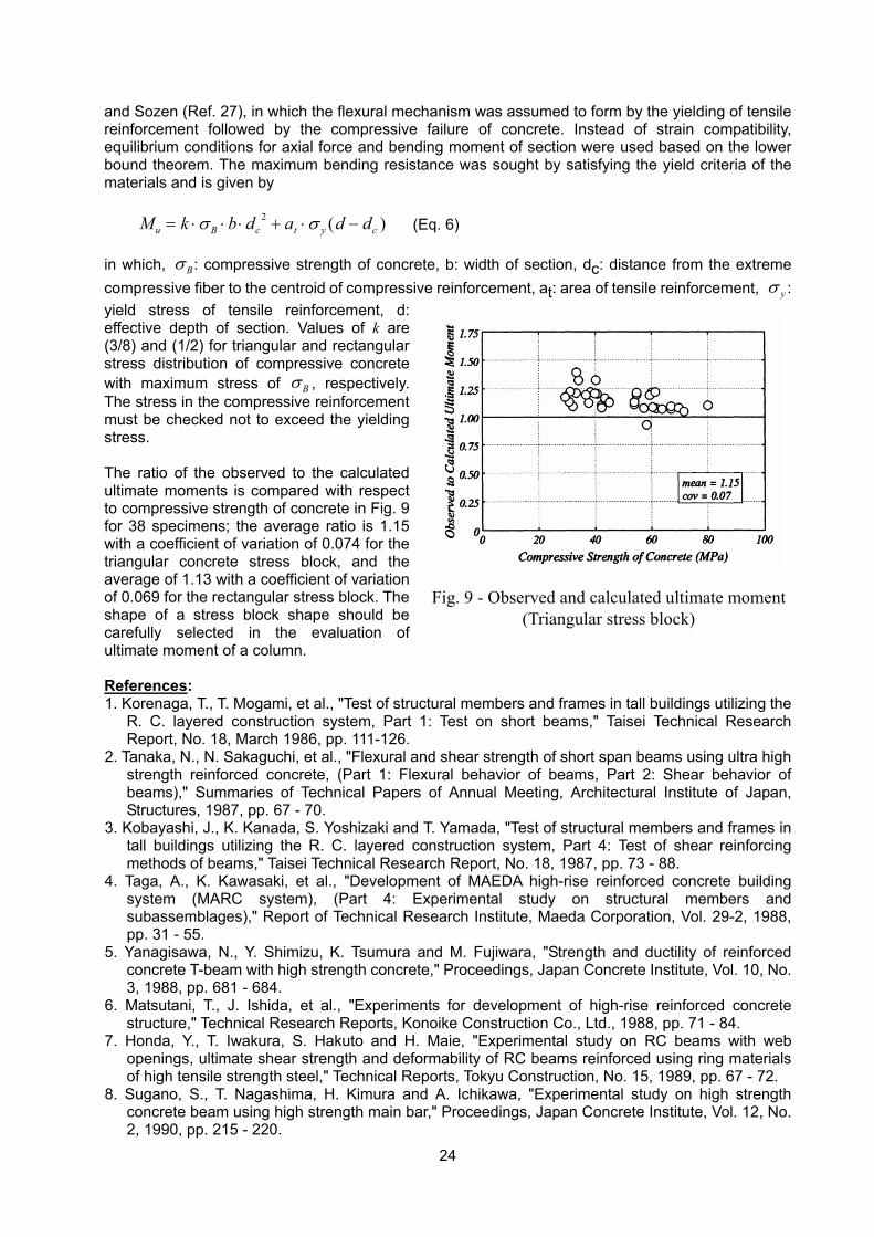
24

and Sozen (Ref. 27), in which the flexural mechanism was assumed to form by the yielding of tensile reinforcement followed by the compressive failure of concrete. Instead of strain compatibility, equilibrium conditions for axial force and bending moment of section were used based on the lower bound theorem. The maximum bending resistance was sought by satisfying the yield criteria of the materials and is given by

M k b d a d du B c t y c= ⋅ ⋅ ⋅ + ⋅ −σ σ2 ( ) (Eq. 6) in which, σB: compressive strength of concrete, b: width of section, dc: distance from the extreme compressive fiber to the centroid of compressive reinforcement, at: area of tensile reinforcement, σ y : yield stress of tensile reinforcement, d: effective depth of section. Values of k are (3/8) and (1/2) for triangular and rectangular stress distribution of compressive concrete with maximum stress of σB , respectively. The stress in the compressive reinforcement must be checked not to exceed the yielding stress. The ratio of the observed to the calculated ultimate moments is compared with respect to compressive strength of concrete in Fig. 9 for 38 specimens; the average ratio is 1.15 with a coefficient of variation of 0.074 for the triangular concrete stress block, and the average of 1.13 with a coefficient of variation of 0.069 for the rectangular stress block. The shape of a stress block shape should be carefully selected in the evaluation of ultimate moment of a column. References: 1. Korenaga, T., T. Mogami, et al., "Test of structural members and frames in tall buildings utilizing the

R. C. layered construction system, Part 1: Test on short beams," Taisei Technical Research Report, No. 18, March 1986, pp. 111-126.

2. Tanaka, N., N. Sakaguchi, et al., "Flexural and shear strength of short span beams using ultra high strength reinforced concrete, (Part 1: Flexural behavior of beams, Part 2: Shear behavior of beams)," Summaries of Technical Papers of Annual Meeting, Architectural Institute of Japan, Structures, 1987, pp. 67 - 70.

3. Kobayashi, J., K. Kanada, S. Yoshizaki and T. Yamada, "Test of structural members and frames in tall buildings utilizing the R. C. layered construction system, Part 4: Test of shear reinforcing methods of beams," Taisei Technical Research Report, No. 18, 1987, pp. 73 - 88.

4. Taga, A., K. Kawasaki, et al., "Development of MAEDA high-rise reinforced concrete building system (MARC system), (Part 4: Experimental study on structural members and subassemblages)," Report of Technical Research Institute, Maeda Corporation, Vol. 29-2, 1988, pp. 31 - 55.

5. Yanagisawa, N., Y. Shimizu, K. Tsumura and M. Fujiwara, "Strength and ductility of reinforced concrete T-beam with high strength concrete," Proceedings, Japan Concrete Institute, Vol. 10, No. 3, 1988, pp. 681 - 684.

6. Matsutani, T., J. Ishida, et al., "Experiments for development of high-rise reinforced concrete structure," Technical Research Reports, Konoike Construction Co., Ltd., 1988, pp. 71 - 84.

7. Honda, Y., T. Iwakura, S. Hakuto and H. Maie, "Experimental study on RC beams with web openings, ultimate shear strength and deformability of RC beams reinforced using ring materials of high tensile strength steel," Technical Reports, Tokyu Construction, No. 15, 1989, pp. 67 - 72.

8. Sugano, S., T. Nagashima, H. Kimura and A. Ichikawa, "Experimental study on high strength concrete beam using high strength main bar," Proceedings, Japan Concrete Institute, Vol. 12, No. 2, 1990, pp. 215 - 220.

Fig. 9 - Observed and calculated ultimate moment

(Triangular stress block)

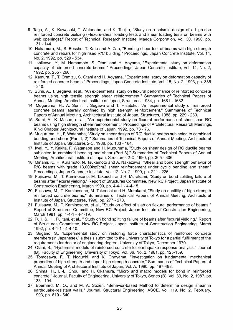
25

9. Taga, A., K. Kawasaki, T. Watanabe, and K. Tsujita, "Study on a seismic design of a high-rise reinforced concrete building (Flexure-shear loading tests and shear loading tests on beams with web openings)," Report of Technical Research Institute, Maeda Corporation, Vol. 30, 1990, pp. 131 - 144.

10. Nakamura, M., S. Bessho, T. Kato and A. Zan, "Bending-shear test of beams with high strength concrete and rebars for high rised R/C building," Proceedings, Japan Concrete Institute, Vol. 14, No. 2, 1992, pp. 529 - 534.

11. Ishikawa, Y., M. Hamamoto, S. Otani and H. Aoyama, "Experimental study on deformation capacity of reinforced concrete beams," Proceedings, Japan Concrete Institute, Vol. 14, No. 2, 1992, pp. 255 - 260.

12. Kamura, T., T. Ohmizu, S. Otani and H. Aoyama, "Experimental study on deformation capacity of reinforced concrete beams," Proceedings, Japan Concrete Institute, Vol. 15, No. 2, 1993, pp. 335 - 340.

13. Sumi, A., T. Segawa, et al., "An experimental study on flexural performance of reinforced concrete beams using high tensile strength shear reinforcement," Summaries of Technical Papers of Annual Meeting, Architectural Institute of Japan, Structures, 1984, pp. 1681 - 1682.

14. Muguruma, H., A. Sumi, T. Segawa and T. Hisatoku, "An experimental study of reinforced concrete beams laterally confined by high strength reinforcement," Summaries of Technical Papers of Annual Meeting, Architectural Institute of Japan, Structures, 1988, pp. 229 - 230.

15. Sumi, A., K. Masuo, et al., "An experimental study on flexural performance of short span RC beams using high strength shear reinforcement," Proceedings of Architectural Research Meetings, Kinki Chapter, Architectural Institute of Japan, 1992, pp. 73 - 76.

16. Muguruma, H., F. Watanabe, "Study on shear design of R/C ductile beams subjected to combined bending and shear (Part 1, 2)," Summaries of Technical Papers of Annual Meeting, Architectural Institute of Japan, Structures 2-C, 1988, pp. 183 - 184.

17. Iwai, Y., Y. Kakita, F. Watanabe and H. Muguruma, "Study on shear design of RC ductile beams subjected to combined bending and shear (Part 3)," Summaries of Technical Papers of Annual Meeting, Architectural Institute of Japan, Structures 2-C, 1990, pp. 305 - 306.

18. Minami, K., H. Kuramoto, N. Tsukamoto and A. Nakazawa, "Shear and bond strength behavior of R/C beams with grade 13,000kgf/cm2 shear reinforcement under cyclic bending and shear," Proceedings, Japan Concrete Institute, Vol. 12, No. 2, 1990, pp. 221 - 226.

19. Fujisawa, M., T. Kaminosono, M. Takeuchi and H. Murakami, "Study on bond splitting failure of beams after flexural yielding," Report of Structures Committee, New RC Project, Japan Institute of Construction Engineering, March 1990, pp. 4-4-1 - 4-4-15.

20. Fujisawa, M., T. Kaminosono, M. Takeuchi and H. Murakami, "Study on ductility of high-strength reinforced concrete beams," Summaries of Technical Papers of Annual Meeting, Architectural Institute of Japan, Structures, 1990, pp. 277 - 278.

21. Fujisawa, M., T. Kaminosono, et al., "Study on effect of slab on flexural performance of beams," Report of Structures Committee, New RC Project, Japan Institute of Construction Engineering, March 1991, pp. 4-4-1 - 4-4-19.

22. Fujii, S., H. Fujitani, et al., " Study on bond splitting failure of beams after flexural yielding," Report of Structures Committee, New RC Project, Japan Institute of Construction Engineering, March 1992, pp. 4-1-1 - 4-4-10.

23. Sugano, S., "Experimental study on restoring force characteristics of reinforced concrete members (in Japanese)," a thesis submitted to the University of Tokyo for a partial fulfillment of the requirements for doctor of engineering degree, University of Tokyo, December 1970.

24. Otani, S., "Hysteresis models of reinforced concrete for earthquake response analysis," Journal (B), Faculty of Engineering, University of Tokyo, Vol. 36, No. 2, 1981, pp. 125-159.

25. Tomosawa, F., T. Noguchi, and K. Onoyama, "Investigation on fundamental mechanical properties of high-strength and super high strength concrete," Summaries of Technical Papers of Annual Meeting of Architectural Institute of Japan, Vol. A, 1990, pp. 497-498.

26. Shima, H., L.-L. Chou, and H. Okamura, "Micro and macro models for bond in reinforced concrete," Journal, Faculty of Engineering, University of Tokyo, Series (B), Vol. 39, No. 2, 1987, pp. 133 - 194.

27. Eberhard, M. O., and M. A. Sozen, "Behavior-based Method to determine design shear in earthquake-resistant walls," Journal, Structural Engineering, ASCE, Vol. 119, No. 2, February, 1993, pp. 619 - 640.

26

4.5 Analysis of Structural Walls

T. Paulay (1981) presents analysis procedures of reinforced concrete structural walls for design purpose. The following deformation should be considered for a structural wall; (a) flexural deformation, (b) shear deformation after diagonal cracking, (c) anchorage deformation, (d) deformation of foundation and supporting ground.

The equivalent second moment eI of area may be taken as 60 % of the value gI based on the

uncracked gross concrete section. A more accurate estimate of flexural deformations may be made if the ratio of the moment causing cracking to the maximum applied moment is evaluated;

3 3

1cr cre g cr

a a

M MI I IM M

= + −

(1)

where, crM : cracking moment, aM : maximum moment at which deflection is computed, gI :

second moment of area of the gross concrete section, crI : moment of inertia of cracked transformed section. The contribution of longitudinal reinforcement can be neglected because the reinforcement ratio is normally less than 0.1 % in a wall.

The elongation of the vertical bars within the foundation structure and slip due to high local bond stresses along the development length will result in an apparent pull-out of such bars at the base of the wall. This can significantly increase the wall deflection.

For cantilever walls with aspect ratios, /w wh l , larger than 4, the shear deformation may be

neglected. After diagonal cracking, however, the shear stiffness is reduced to 10 - 30 % of the uncracked stiffness. The lateral reinforcement influences the shear deformation after diagonal cracking.

When the aspect ratio is less than 4, the second moment of area for a structural wall may be

assumed that

2

1.230

ew

e

w w w

IIF

IFh b

=+

=l

(2)

In this expression, some allowance is made for shear distortions and deflections due to anchorage (pull-out) deformation at the base of a wall.

The structural wall tests at Portland Cement Association were examined. The aspect ratio of the specimens was 2.4. Cross sections were flanged (H-shape), barbell (with boundary columns) and rectangular. Equation (1) tends to overestimate the initial stiffness.

For a cantilever wall, the wall may be represented by a straight line passing through the centroid

of the gross section.. Reference: Paulay, T., “The Design of Reinforced Concrete Ductile Shear Walls for Earthquake

Resistance,“ Research Report 81-1, Department of Civil Engineering, University of Canterbury, New Zealand, February 1981, 72 pp.

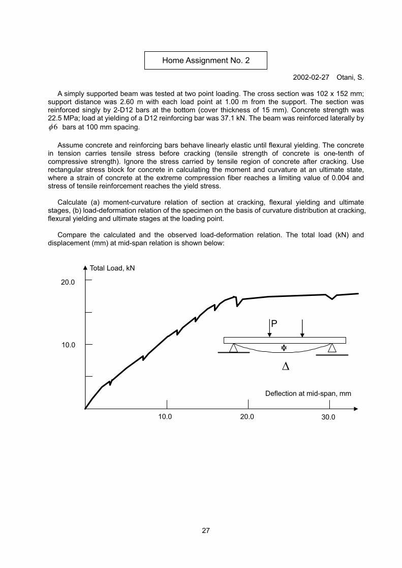
27

Home Assignment No. 2

2002-02-27 Otani, S.

A simply supported beam was tested at two point loading. The cross section was 102 x 152 mm;

support distance was 2.60 m with each load point at 1.00 m from the support. The section was reinforced singly by 2-D12 bars at the bottom (cover thickness of 15 mm). Concrete strength was 22.5 MPa; load at yielding of a D12 reinforcing bar was 37.1 kN. The beam was reinforced laterally by

6φ bars at 100 mm spacing. Assume concrete and reinforcing bars behave linearly elastic until flexural yielding. The concrete

in tension carries tensile stress before cracking (tensile strength of concrete is one-tenth of compressive strength). Ignore the stress carried by tensile region of concrete after cracking. Use rectangular stress block for concrete in calculating the moment and curvature at an ultimate state, where a strain of concrete at the extreme compression fiber reaches a limiting value of 0.004 and stress of tensile reinforcement reaches the yield stress.

Calculate (a) moment-curvature relation of section at cracking, flexural yielding and ultimate

stages, (b) load-deformation relation of the specimen on the basis of curvature distribution at cracking, flexural yielding and ultimate stages at the loading point.

Compare the calculated and the observed load-deformation relation. The total load (kN) and

displacement (mm) at mid-span relation is shown below:

10.0 20.0 30.0

Deflection at mid-span, mm

Total Load, kN

20.0

10.0

∆

P

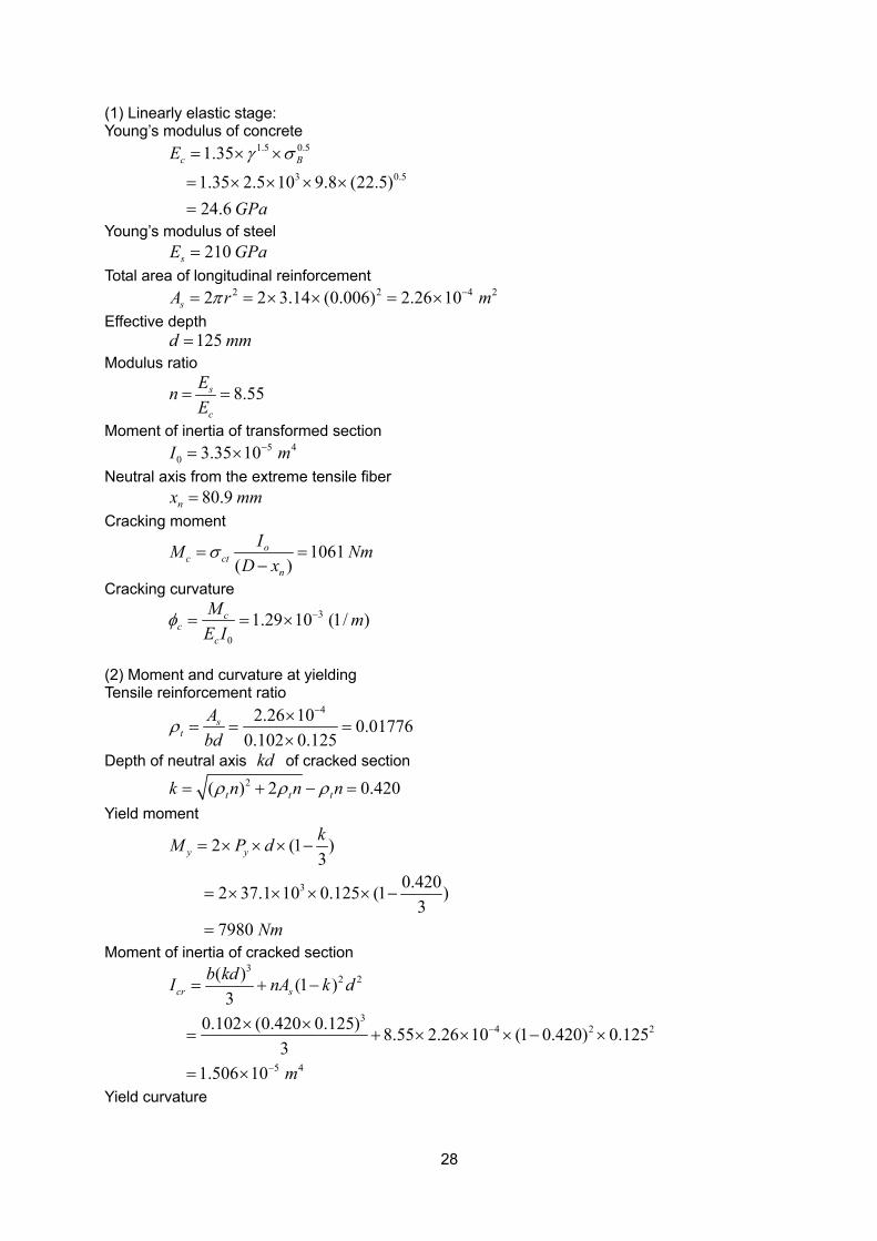
28

(1) Linearly elastic stage: Young’s modulus of concrete

1.5 0.5

3 0.5

1.35

1.35 2.5 10 9.8 (22.5)24.6

c BE

GPa

γ σ= × ×

= × × × ×=

Young’s modulus of steel 210sE GPa= Total area of longitudinal reinforcement 2 2 4 22 2 3.14 (0.006) 2.26 10sA r mπ −= = × × = × Effective depth 125d mm= Modulus ratio

8.55s

c

EnE

= =

Moment of inertia of transformed section 5 4

0 3.35 10I m−= × Neutral axis from the extreme tensile fiber 80.9nx mm= Cracking moment

1061( )

oc ct

n

IM NmD x

σ= =−

Cracking curvature

3

0

1.29 10 (1/ )cc

c

M mE I

φ −= = ×

(2) Moment and curvature at yielding Tensile reinforcement ratio

42.26 10 0.01776

0.102 0.125s

tAbd

ρ−×

= = =×

Depth of neutral axis kd of cracked section

2( ) 2 0.420t t tk n n nρ ρ ρ= + − = Yield moment

3

2 (1 )3

0.4202 37.1 10 0.125 (1 )3

7980

y ykM P d

Nm

= × × × −

= × × × × −

=

Moment of inertia of cracked section

32 2

34 2 2

5 4

( ) (1 )3

0.102 (0.420 0.125) 8.55 2.26 10 (1 0.420) 0.1253

1.506 10

cr sb kdI nA k d

m

−

−

= + −

× ×= + × × × − ×

= ×

Yield curvature

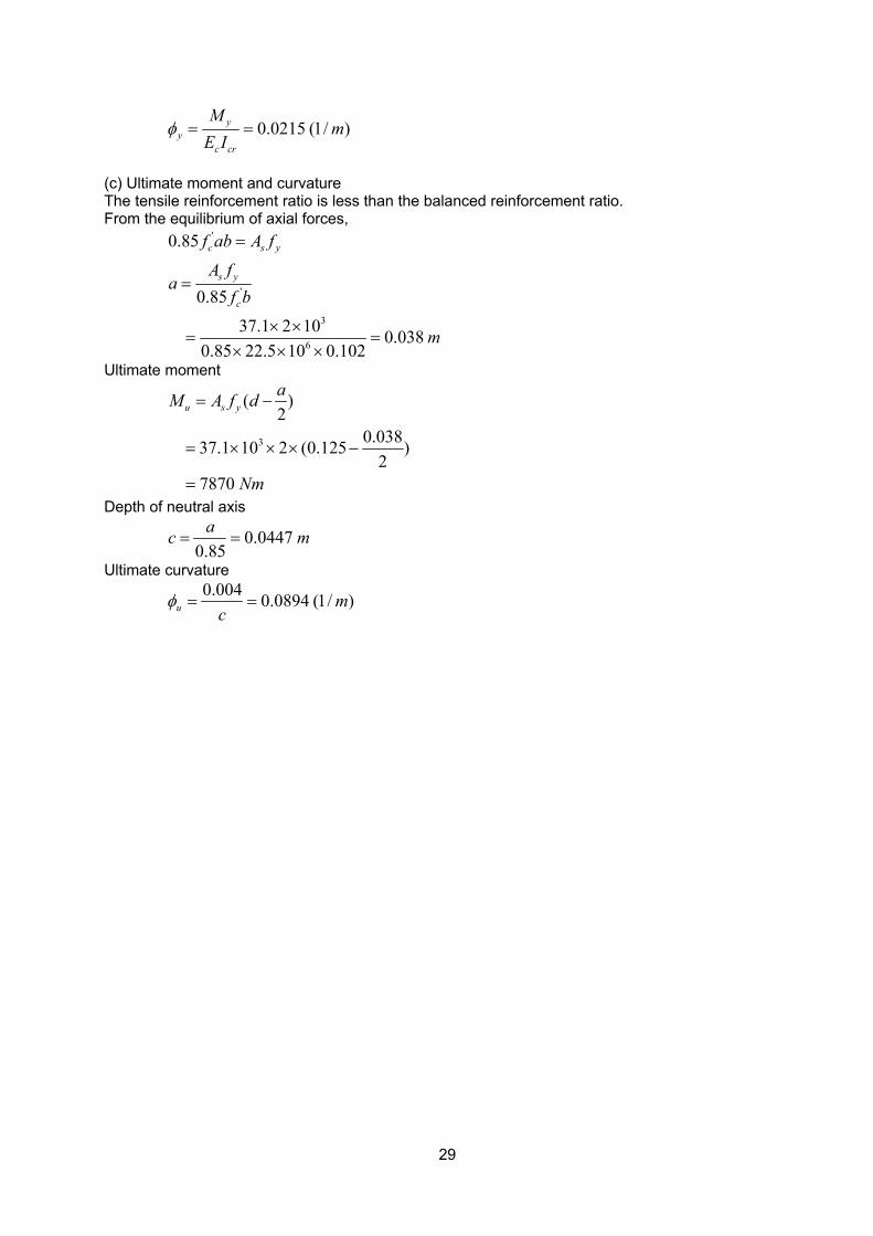
29

0.0215 (1/ )yy

c cr

Mm

E Iφ = =

(c) Ultimate moment and curvature The tensile reinforcement ratio is less than the balanced reinforcement ratio. From the equilibrium of axial forces,

'

'

3

6

0.85

0.85

37.1 2 10 0.0380.85 22.5 10 0.102

c s y

s y

c

f ab A fA f

af b

m

=

=

× ×= =

× × ×

Ultimate moment

3

( )2

0.03837.1 10 2 (0.125 )2

7870

u s yaM A f d

Nm

= −

= × × × −

=

Depth of neutral axis

0.04470.85

ac m= =

Ultimate curvature

0.004 0.0894 (1/ )u m

cφ = =

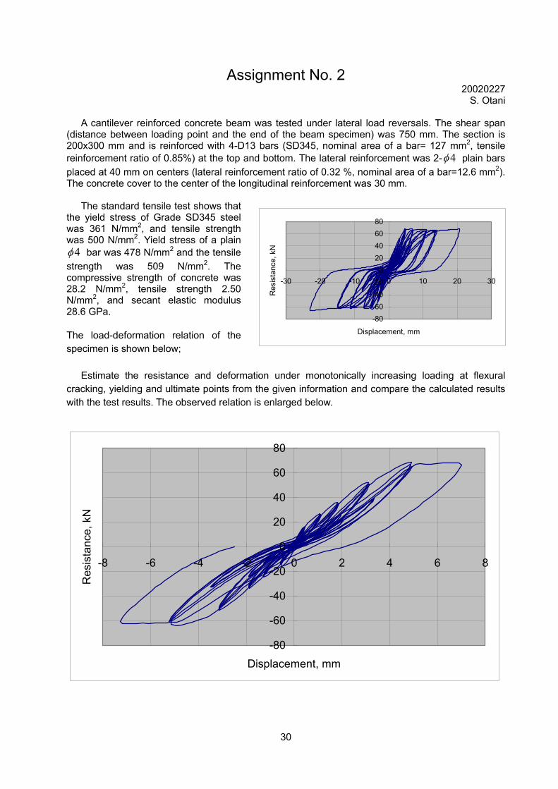
30

Assignment No. 2 20020227

S. Otani

A cantilever reinforced concrete beam was tested under lateral load reversals. The shear span (distance between loading point and the end of the beam specimen) was 750 mm. The section is 200x300 mm and is reinforced with 4-D13 bars (SD345, nominal area of a bar= 127 mm2, tensile reinforcement ratio of 0.85%) at the top and bottom. The lateral reinforcement was 2- 4φ plain bars placed at 40 mm on centers (lateral reinforcement ratio of 0.32 %, nominal area of a bar=12.6 mm2). The concrete cover to the center of the longitudinal reinforcement was 30 mm.

The standard tensile test shows that the yield stress of Grade SD345 steel was 361 N/mm2, and tensile strength was 500 N/mm2. Yield stress of a plain

4φ bar was 478 N/mm2 and the tensile strength was 509 N/mm2. The compressive strength of concrete was 28.2 N/mm2, tensile strength 2.50 N/mm2, and secant elastic modulus 28.6 GPa. The load-deformation relation of the specimen is shown below;

Estimate the resistance and deformation under monotonically increasing loading at flexural cracking, yielding and ultimate points from the given information and compare the calculated results with the test results. The observed relation is enlarged below.

-80

-60

-40

-20

0

20

40

60

80

-8 -6 -4 -2 0 2 4 6 8

Displacement, mm

Res

ista

nce,

kN

-80-60-40-20

020406080

-30 -20 -10 0 10 20 30

Displacement, mm

Res

ista

nce,

kN

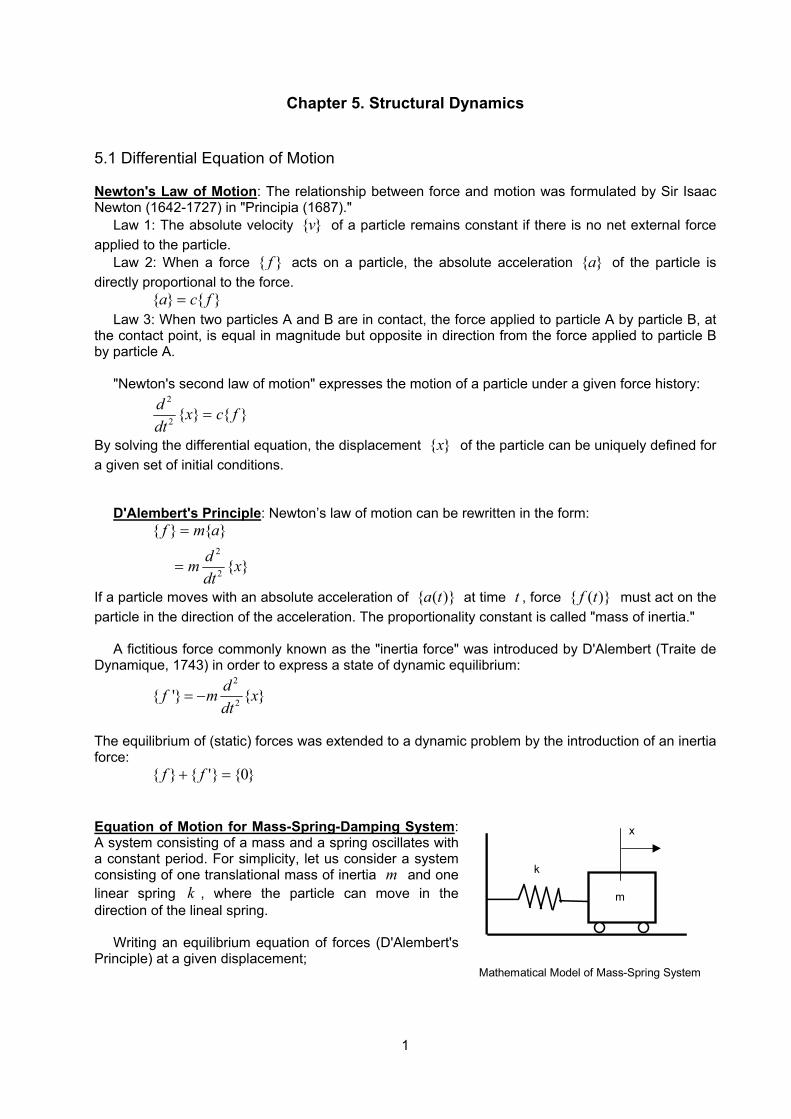
1

Chapter 5. Structural Dynamics 5.1 Differential Equation of Motion Newton's Law of Motion: The relationship between force and motion was formulated by Sir Isaac Newton (1642-1727) in "Principia (1687)."

Law 1: The absolute velocity }{v of a particle remains constant if there is no net external force applied to the particle.

Law 2: When a force { }f acts on a particle, the absolute acceleration }{a of the particle is directly proportional to the force.

}{}{ fca = Law 3: When two particles A and B are in contact, the force applied to particle A by particle B, at

the contact point, is equal in magnitude but opposite in direction from the force applied to particle B by particle A.

"Newton's second law of motion" expresses the motion of a particle under a given force history:

}{}{22

fcxdtd

=

By solving the differential equation, the displacement }{x of the particle can be uniquely defined for a given set of initial conditions.

D'Alembert's Principle: Newton’s law of motion can be rewritten in the form:

}{

}{}{

2

2

xdtdm

amf

=

=

If a particle moves with an absolute acceleration of )}({ ta at time t , force )}({ tf must act on the particle in the direction of the acceleration. The proportionality constant is called "mass of inertia."

A fictitious force commonly known as the "inertia force" was introduced by D'Alembert (Traite de Dynamique, 1743) in order to express a state of dynamic equilibrium:

2

2{ '} { }df m xdt

= −

The equilibrium of (static) forces was extended to a dynamic problem by the introduction of an inertia force:

}0{}'{}{ =+ ff Equation of Motion for Mass-Spring-Damping System: A system consisting of a mass and a spring oscillates with a constant period. For simplicity, let us consider a system consisting of one translational mass of inertia m and one linear spring k , where the particle can move in the direction of the lineal spring.

Writing an equilibrium equation of forces (D'Alembert's Principle) at a given displacement;

Mathematical Model of Mass-Spring System

m

k

x

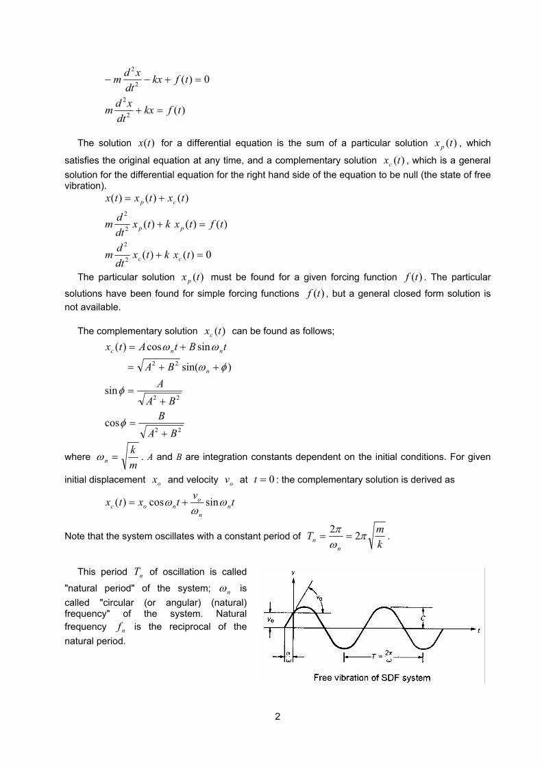
2

)(

0)(

2

2

2

2

tfkxdtxdm

tfkxdtxdm

=+

=+−−

The solution )(tx for a differential equation is the sum of a particular solution )(tx p , which

satisfies the original equation at any time, and a complementary solution )(txc , which is a general solution for the differential equation for the right hand side of the equation to be null (the state of free vibration).

0)()(

)()()(

)()()(

2

2

2

2

=+

=+

+=

txktxdtdm

tftxktxdtdm

txtxtx

cc

pp

cp

The particular solution )(tx p must be found for a given forcing function )(tf . The particular

solutions have been found for simple forcing functions )(tf , but a general closed form solution is not available.

The complementary solution )(txc can be found as follows;

22

22

22

cos

sin

)sin(

sincos)(

BABBA

ABA

tBtAtx

n

nnc

+=

+=

++=

+=

φ

φ

φω

ωω

where mk

n =ω . A and B are integration constants dependent on the initial conditions. For given

initial displacement ox and velocity ov at 0=t : the complementary solution is derived as

tvtxtx nn

onoc ω

ωω sincos)( +=

Note that the system oscillates with a constant period of kmT

nn π

ωπ 22== .

This period nT of oscillation is called

"natural period" of the system; nω is called "circular (or angular) (natural) frequency" of the system. Natural frequency nf is the reciprocal of the natural period.

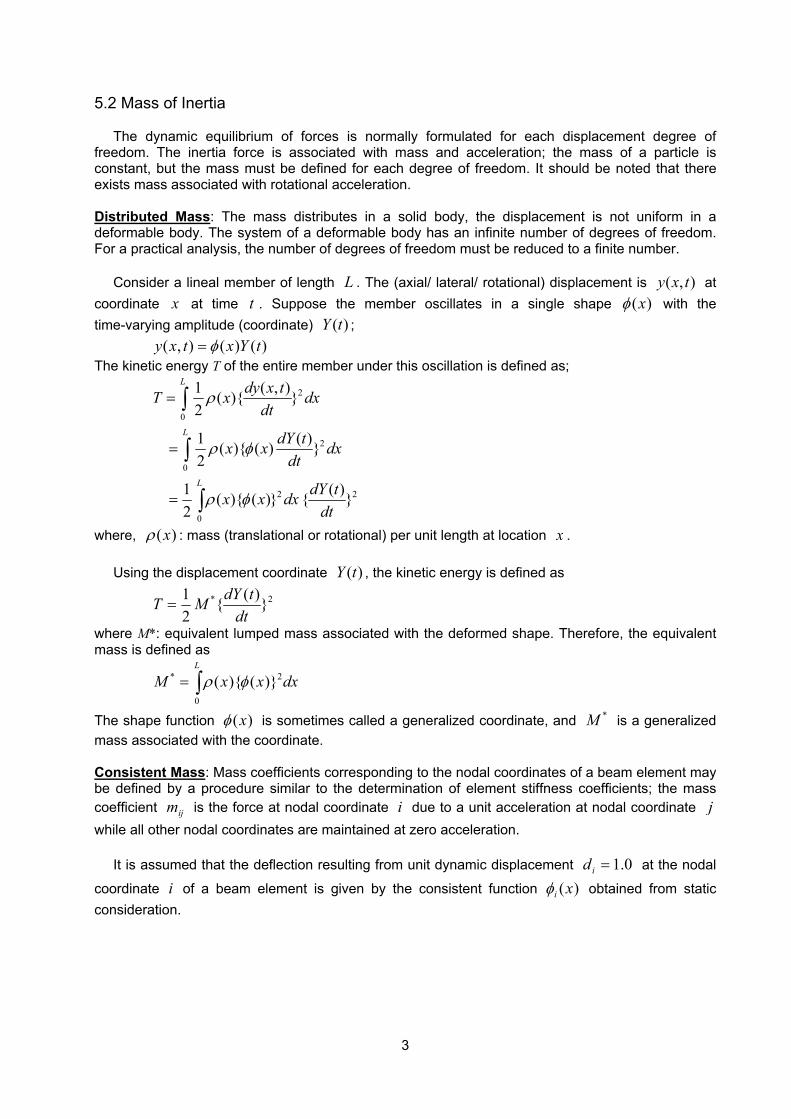
3

5.2 Mass of Inertia

The dynamic equilibrium of forces is normally formulated for each displacement degree of freedom. The inertia force is associated with mass and acceleration; the mass of a particle is constant, but the mass must be defined for each degree of freedom. It should be noted that there exists mass associated with rotational acceleration. Distributed Mass: The mass distributes in a solid body, the displacement is not uniform in a deformable body. The system of a deformable body has an infinite number of degrees of freedom. For a practical analysis, the number of degrees of freedom must be reduced to a finite number.

Consider a lineal member of length L . The (axial/ lateral/ rotational) displacement is ),( txy at coordinate x at time t . Suppose the member oscillates in a single shape )(xφ with the time-varying amplitude (coordinate) )(tY ; )()(),( tYxtxy φ= The kinetic energy T of the entire member under this oscillation is defined as;

2

0

2

0

2 2

0

1 ( , )( ){ }2

1 ( )( ){ ( ) }2

1 ( )( ){ ( )} { }2

L

L

L

dy x tT x dxdt

dY tx x dxdt

dY tx x dxdt

ρ

ρ φ

ρ φ

=

=

=

∫

∫

∫

where, )(xρ : mass (translational or rotational) per unit length at location x .

Using the displacement coordinate )(tY , the kinetic energy is defined as

2* })({21

dttdYMT =

where M*: equivalent lumped mass associated with the deformed shape. Therefore, the equivalent mass is defined as

dxxxML

∫=0

2* )}(){( φρ

The shape function )(xφ is sometimes called a generalized coordinate, and *M is a generalized mass associated with the coordinate. Consistent Mass: Mass coefficients corresponding to the nodal coordinates of a beam element may be defined by a procedure similar to the determination of element stiffness coefficients; the mass coefficient ijm is the force at nodal coordinate i due to a unit acceleration at nodal coordinate j while all other nodal coordinates are maintained at zero acceleration.

It is assumed that the deflection resulting from unit dynamic displacement 0.1=id at the nodal

coordinate i of a beam element is given by the consistent function )(xiφ obtained from static consideration.

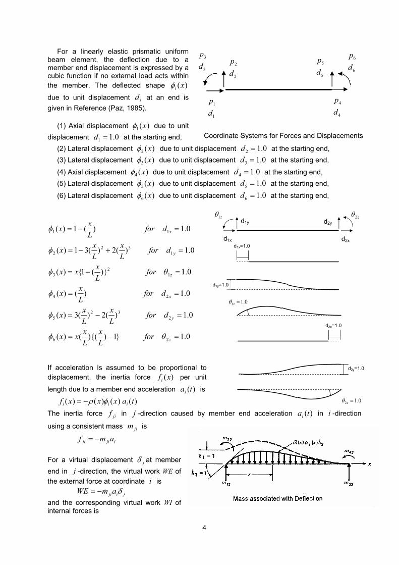
4

For a linearly elastic prismatic uniform beam element, the deflection due to a member end displacement is expressed by a cubic function if no external load acts within the member. The deflected shape )(xiφ

due to unit displacement id at an end is given in Reference (Paz, 1985).

(1) Axial displacement )(1 xφ due to unit

displacement 0.11 =d at the starting end, (2) Lateral displacement )(2 xφ due to unit displacement 0.12 =d at the starting end, (3) Lateral displacement )(3 xφ due to unit displacement 0.13 =d at the starting end,

(4) Axial displacement )(4 xφ due to unit displacement 0.14 =d at the starting end, (5) Lateral displacement )(5 xφ due to unit displacement 0.15 =d at the starting end,

(6) Lateral displacement )(6 xφ due to unit displacement 0.16 =d at the starting end,

0.1}1)){(()(

0.1)(2)(3)(

0.1)()(

0.1)}(1{)(

0.1)(2)(31)(

0.1)(1)(

26

232

5

24

12

3

132

2

11

=−=

=−=

==

=−=

=+−=

=−=

z

y

x

z

y

x

forLx

Lxxx

dforLx

Lxx

dforLxx

forLxxx

dforLx

Lxx

dforLxx

θφ

φ

φ

θφ

φ

φ

If acceleration is assumed to be proportional to displacement, the inertia force )(xfi per unit

length due to a member end acceleration )(tai is

)()()()( taxxxf iii φρ−=

The inertia force jif in j -direction caused by member end acceleration )(tai in i -direction

using a consistent mass jim is

ijiji amf −= For a virtual displacement jδ at member end in j -direction, the virtual work WE of the external force at coordinate i is jijiamWE δ−= and the corresponding virtual work WI of internal forces is

3

3

dp

6

6

dp

1

1

dp

2

2

dp

5

5

dp

4

4

dp

Coordinate Systems for Forces and Displacements

d1x

d1y

d2x

d2y1zθ 2 zθ

d1x=1.0

d1y=1.0

1 1.0zθ =

d2x=1.0

d2y=1.0

2 1.0zθ =

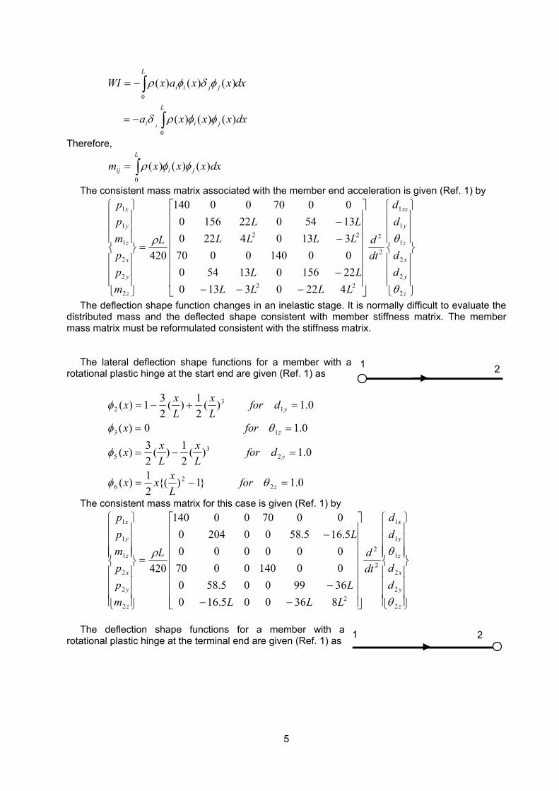
5

∫

∫

−=

−=

L

jii

L

jjii

dxxxxa

dxxxaxWI

j

0

0

)()()(

)()()(

φφρδ

φδφρ

Therefore,

∫=L

jiij dxxxxm0

)()()( φφρ

The consistent mass matrix associated with the member end acceleration is given (Ref. 1) by

−−−−

−−

=

z

y

x

z

y

xx

z

y

x

z

y

x

dd

dd

dtd

LLLLLL

LLLLLL

L

mppmpp

2

2

2

1

1

1

2

2

22

22

2

2

2

1

1

1

42203130221560135400014000703130422013540221560007000140

420

θ

θρ

The deflection shape function changes in an inelastic stage. It is normally difficult to evaluate the distributed mass and the deflected shape consistent with member stiffness matrix. The member mass matrix must be reformulated consistent with the stiffness matrix.

The lateral deflection shape functions for a member with a rotational plastic hinge at the start end are given (Ref. 1) as

0.1}1){(21)(

0.1)(21)(

23)(

0.10)(

0.1)(21)(

231)(

22

6

23

5

13

13

2

=−=

=−=

==

=+−=

z

y

z

y

forLxxx

dforLx

Lxx

forx

dforLx

Lxx

θφ

φ

θφ

φ

The consistent mass matrix for this case is given (Ref. 1) by

−−−

−

=

z

y

x

z

y

x

z

y

x

z

y

x

dd

dd

dtd

LLLL

LL

mppmpp

2

2

2

1

1

1

2

2

22

2

2

1

1

1

836005.1603699005.5800014000700000005.165.58002040007000140

420

θ

θρ

The deflection shape functions for a member with a

rotational plastic hinge at the terminal end are given (Ref. 1) as

1 2

1 2

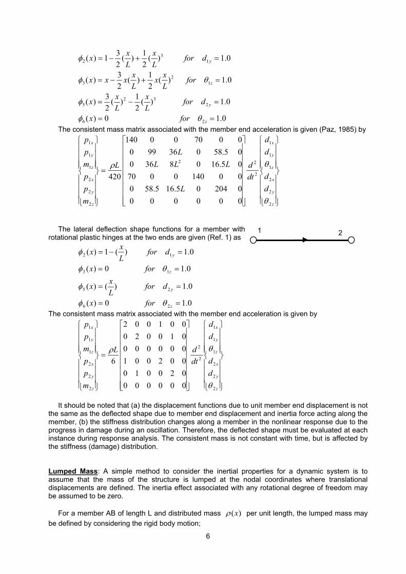
6

0.10)(

0.1)(21)(

23)(

0.1)(21)(

23)(

0.1)(21)(

231)(

26

232

5

12

3

13

2

==

=−=

=+−=

=+−=

z

y

z

y

forx

dforLx

Lxx

forLxx

Lxxxx

dforLx

Lxx

θφ

φ

θφ

φ

The consistent mass matrix associated with the member end acceleration is given (Paz, 1985) by

=

z

y

x

z

y

x

z

y

x

z

y

x

dd

dd

dtd

L

LLLL

L

mppmpp

2

2

2

1

1

1

2

22

2

2

2

1

1

1

000000020405.165.58000140007005.160836005.58036990007000140

420

θ

θρ

The lateral deflection shape functions for a member with rotational plastic hinges at the two ends are given (Ref. 1) as

0.10)(

0.1)()(

0.10)(

0.1)(1)(

26

25

13

12

==

==

==

=−=

z

y

z

y

forx

dforLxx

forx

dforLxx

θφ

φ

θφ

φ

The consistent mass matrix associated with the member end acceleration is given by

=

z

y

x

z

y

x

z

y

x

z

y

x

dd

dd

dtdL

mppmpp

2

2

2

1

1

1

2

2

2

2

2

1

1

1

000000020010002001000000010020001002

6

θ

θρ

It should be noted that (a) the displacement functions due to unit member end displacement is not

the same as the deflected shape due to member end displacement and inertia force acting along the member, (b) the stiffness distribution changes along a member in the nonlinear response due to the progress in damage during an oscillation. Therefore, the deflected shape must be evaluated at each instance during response analysis. The consistent mass is not constant with time, but is affected by the stiffness (damage) distribution. Lumped Mass: A simple method to consider the inertial properties for a dynamic system is to assume that the mass of the structure is lumped at the nodal coordinates where translational displacements are defined. The inertia effect associated with any rotational degree of freedom may be assumed to be zero.

For a member AB of length L and distributed mass )(xρ per unit length, the lumped mass may be defined by considering the rigid body motion;

1 2

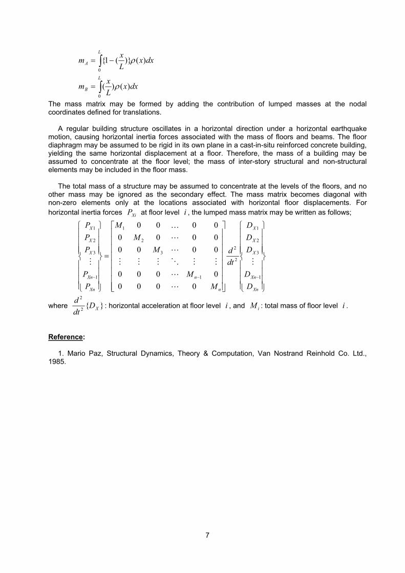
7

dxxLxm

dxxLxm

L

B

L

A

)()(

)()}(1{

0

0

ρ

ρ

∫

∫

=

−=

The mass matrix may be formed by adding the contribution of lumped masses at the nodal coordinates defined for translations.

A regular building structure oscillates in a horizontal direction under a horizontal earthquake motion, causing horizontal inertia forces associated with the mass of floors and beams. The floor diaphragm may be assumed to be rigid in its own plane in a cast-in-situ reinforced concrete building, yielding the same horizontal displacement at a floor. Therefore, the mass of a building may be assumed to concentrate at the floor level; the mass of inter-story structural and non-structural elements may be included in the floor mass.

The total mass of a structure may be assumed to concentrate at the levels of the floors, and no other mass may be ignored as the secondary effect. The mass matrix becomes diagonal with non-zero elements only at the locations associated with horizontal floor displacements. For horizontal inertia forces XiP at floor level i , the lumped mass matrix may be written as follows;

=

−−−

Xn

Xn

X

X

X

n

n

Xn

Xn

X

X

X

DD

DDD

dtd

MM

MM

M

PP

PPP

1

3

2

1

2

2

1

3

2

1

1

3

2

1

00000000

000000000000

M

L

L

MMOMMM

L

L

K

M

where }{22

XDdtd

: horizontal acceleration at floor level i , and iM : total mass of floor level i .

Reference:

1. Mario Paz, Structural Dynamics, Theory & Computation, Van Nostrand Reinhold Co. Ltd., 1985.

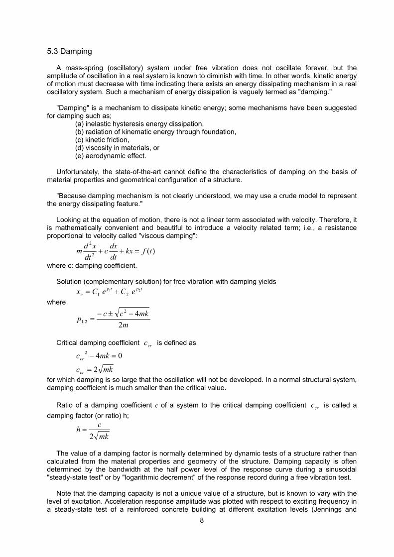
8

5.3 Damping

A mass-spring (oscillatory) system under free vibration does not oscillate forever, but the amplitude of oscillation in a real system is known to diminish with time. In other words, kinetic energy of motion must decrease with time indicating there exists an energy dissipating mechanism in a real oscillatory system. Such a mechanism of energy dissipation is vaguely termed as "damping."

"Damping" is a mechanism to dissipate kinetic energy; some mechanisms have been suggested for damping such as; (a) inelastic hysteresis energy dissipation, (b) radiation of kinematic energy through foundation, (c) kinetic friction, (d) viscosity in materials, or (e) aerodynamic effect.

Unfortunately, the state-of-the-art cannot define the characteristics of damping on the basis of material properties and geometrical configuration of a structure.

"Because damping mechanism is not clearly understood, we may use a crude model to represent the energy dissipating feature."

Looking at the equation of motion, there is not a linear term associated with velocity. Therefore, it is mathematically convenient and beautiful to introduce a velocity related term; i.e., a resistance proportional to velocity called "viscous damping":

)(2

2

tfkxdtdxc

dtxdm =++

where c: damping coefficient.

Solution (complementary solution) for free vibration with damping yields tptp

c eCeCx 2121 +=

where

mmkccp

242

2,1−±−

=

Critical damping coefficient crc is defined as

mkc

mkc

cr

cr

2

042

=

=−

for which damping is so large that the oscillation will not be developed. In a normal structural system, damping coefficient is much smaller than the critical value.

Ratio of a damping coefficient c of a system to the critical damping coefficient crc is called a damping factor (or ratio) h;

mkch

2=

The value of a damping factor is normally determined by dynamic tests of a structure rather than

calculated from the material properties and geometry of the structure. Damping capacity is often determined by the bandwidth at the half power level of the response curve during a sinusoidal "steady-state test" or by "logarithmic decrement" of the response record during a free vibration test.

Note that the damping capacity is not a unique value of a structure, but is known to vary with the level of excitation. Acceleration response amplitude was plotted with respect to exciting frequency in a steady-state test of a reinforced concrete building at different excitation levels (Jennings and

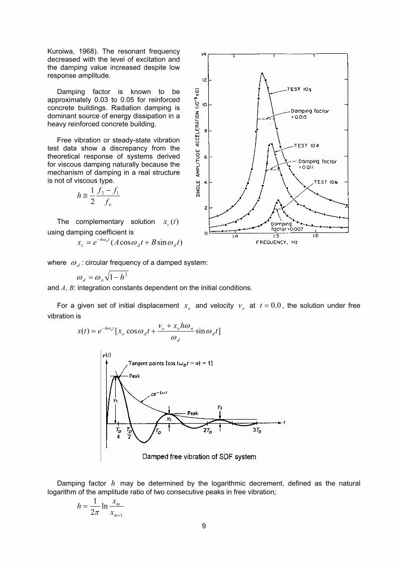
9

Kuroiwa, 1968). The resonant frequency decreased with the level of excitation and the damping value increased despite low response amplitude.

Damping factor is known to be approximately 0.03 to 0.05 for reinforced concrete buildings. Radiation damping is dominant source of energy dissipation in a heavy reinforced concrete building.

Free vibration or steady-state vibration test data show a discrepancy from the theoretical response of systems derived for viscous damping naturally because the mechanism of damping in a real structure is not of viscous type.

nfffh 12

21 −

≅

The complementary solution )(txc

using damping coefficient is )sincos( tBtAex dd

thc

n ωωω += −

where dω : circular frequency of a damped system:

21 hnd −=ωω and A, B: integration constants dependent on the initial conditions.

For a given set of initial displacement ox and velocity ov at 0.0=t , the solution under free vibration is

]sincos[)( thxv

txetx dd

noodo

th n ωω

ωωω +

+= −

Damping factor h may be determined by the logarithmic decrement, defined as the natural

logarithm of the amplitude ratio of two consecutive peaks in free vibration;

1

ln21

+

=m

m

xxh

π

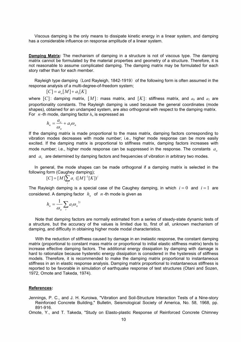
10

Viscous damping is the only means to dissipate kinetic energy in a linear system, and damping

has a considerable influence on response amplitude of a linear system.

Damping Matrix: The mechanism of damping in a structure is not of viscous type. The damping matrix cannot be formulated by the material properties and geometry of a structure. Therefore, it is not reasonable to assume complicated damping. The damping matrix may be formulated for each story rather than for each member.

Rayleigh type damping （Lord Rayleigh, 1842-1919） of the following form is often assumed in the

response analysis of a multi-degree-of-freedom system; ][][][ 1 KaMaC o += where ][C : damping matrix, ][M : mass matrix, and ][K : stiffness matrix, and a0 and a1 are proportionality constants. The Rayleigh damping is used because the general coordinates (mode shapes), obtained for an undamped system, are also orthogonal with respect to the damping matrix. For n -th mode, damping factor hn is expressed as

nn

on aah ω

ω 1+=

If the damping matrix is made proportional to the mass matrix, damping factors corresponding to vibration modes decreases with mode number; i.e., higher mode response can be more easily excited. If the damping matrix is proportional to stiffness matrix, damping factors increases with mode number; i.e., higher mode response can be suppressed in the response. The constants oa

and 1a are determined by damping factors and frequencies of vibration in arbitrary two modes.

In general, the mode shapes can be made orthogonal if a damping matrix is selected in the following form (Caughey damping); ∑ −=

i

ii KMaMC ])[]([][][ 1

The Rayleigh damping is a special case of the Caughey damping, in which 0=i and 1=i are considered. A damping factor nh of n -th mode is given as

in

ii

nn ah 21 ω

ω ∑=

Note that damping factors are normally estimated from a series of steady-state dynamic tests of

a structure, but the accuracy of the values is limited due to, first of all, unknown mechanism of damping, and difficulty in obtaining higher mode modal characteristics.

With the reduction of stiffness caused by damage in en inelastic response, the constant damping matrix (proportional to constant mass matrix or proportional to initial elastic stiffness matrix) tends to increase effective damping factors. The additional energy dissipation by damping with damage is hard to rationalize because hysteretic energy dissipation is considered in the hysteresis of stiffness models. Therefore, it is recommended to make the damping matrix proportional to instantaneous stiffness in an in elastic response analysis. Damping matrix proportional to instantaneous stiffness is reported to be favorable in simulation of earthquake response of test structures (Otani and Sozen, 1972, Omote and Takeda, 1974). References: Jennings, P. C., and J. H. Kuroiwa, "Vibration and Soil-Structure Interaction Tests of a Nine-story

Reinforced Concrete Building," Bulletin, Seismological Society of America, No. 58, 1968, pp. 891-916.

Omote, Y., and T. Takeda, "Study on Elasto-plastic Response of Reinforced Concrete Chimney

11

(Part 1: Model Test) (in Japanese)," Transactions, Architectural Institute of Japan, No. 215, January 1974, pp. 21-32.

Otani, S., and M. A. Sozen, "Behavior of Multistory Reinforced Concrete Frame Structures," Civil Engineering Studies, Structural Research Series No. 392, University of Illinois, 1972.

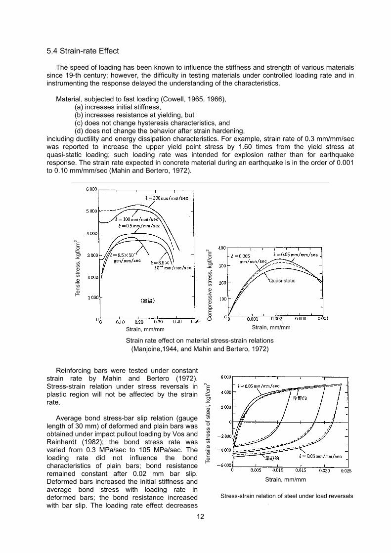
12

5.4 Strain-rate Effect

The speed of loading has been known to influence the stiffness and strength of various materials since 19-th century; however, the difficulty in testing materials under controlled loading rate and in instrumenting the response delayed the understanding of the characteristics.

Material, subjected to fast loading (Cowell, 1965, 1966), (a) increases initial stiffness, (b) increases resistance at yielding, but (c) does not change hysteresis characteristics, and (d) does not change the behavior after strain hardening, including ductility and energy dissipation characteristics. For example, strain rate of 0.3 mm/mm/sec was reported to increase the upper yield point stress by 1.60 times from the yield stress at quasi-static loading; such loading rate was intended for explosion rather than for earthquake response. The strain rate expected in concrete material during an earthquake is in the order of 0.001 to 0.10 mm/mm/sec (Mahin and Bertero, 1972).

Strain rate effect on material stress-strain relations (Manjoine,1944, and Mahin and Bertero, 1972)

Strain, mm/mm Strain, mm/mm

Tens

ile s

tress

, kgf

/cm

2

Com

pres

sive

stre

ss, k

gf/c

m2

Quasi-static

Reinforcing bars were tested under constant

strain rate by Mahin and Bertero (1972). Stress-strain relation under stress reversals in plastic region will not be affected by the strain rate.

Average bond stress-bar slip relation (gauge length of 30 mm) of deformed and plain bars was obtained under impact pullout loading by Vos and Reinhardt (1982); the bond stress rate was varied from 0.3 MPa/sec to 105 MPa/sec. The loading rate did not influence the bond characteristics of plain bars; bond resistance remained constant after 0.02 mm bar slip. Deformed bars increased the initial stiffness and average bond stress with loading rate in deformed bars; the bond resistance increased with bar slip. The loading rate effect decreases

Strain, mm/mm

Tens

ile s

tress

of s

teel

, kgf

/cm

2

Stress-strain relation of steel under load reversals

13

with strength of concrete. The difference in the loading rate effect on deformed bars and plain bars might be interpreted that chemical adhesion bond resistance is not influenced by loading rate, but mechanical interlocking bond resistance is influenced by the loading rate.

Tests of reinforced concrete members at constant velocity of 0.002 rad/sec and 0.2 rad/sec of member rotational velocity (Mahin and Bertero, 1972) indicated that

(a) high strain rates increased the initial yield resistance, but caused small differences in either stiffness or resistance in subsequent cycles at the same displacement amplitudes,

(b) strain rate effect on resistance diminished with increased deformation in a strain-hardening range, and

(c) no substantial changes were observed in ductility and overall energy absorption capacity.

Earthquake simulator tests of reinforced concrete members and structural models have been successfully simulated by analysis on the basis of hysteresis model developed on the basis of force-deformation relationship observed in static laboratory tests (Takeda, Nielsen and Sozen, 1970, Otani and Sozen, 1972, Koike, Omote and Takeda, 1980,).

Displacement, cm Displacement, cm

Res

ista

nce,

tonf

Res

ista

nce,

tonf

Note that strain rate (velocity) during an oscillation is highest at low stress levels, and that the rate

gradually decreases toward a peak strain (displacement). Damage in the reinforced concrete reduces the stiffness, elongating the period of oscillation. Furthermore, such damage is caused normally by lower modes of oscillation having longer periods. Therefore, the strain rate effect can be judged small on the earthquake response of a normal reinforced concrete structure.

Bar slip

Bar slip, mm

Aver

age

bond

stre

ss, k

gf/c

m2

Bond stress speed

Bar slip, mm Aver

age

bond

stre

ss, k

gf/c

m2

Average bond stress-bar slip relation for D10 bars (vos and Reinhardt, 1982)

Bond stress speed

14

References: Cowell, W. L., "Dynamic Tests of Concrete Reinforcing Steels," Technical Report No. 394, U.S.

Naval Civil Engineering Laboratory, Port Hueneme, California, 1965. Cowell, W. L., "Dynamic Properties of Plain Portland Cement Concrete," Technical Report No. 447,

U.S. Naval Civil Engineering Laboratory, Port Hueneme, California, 1966. Koike, K., Y. Omote and T. Takeda, "Reinforced Concrete Wall-Frame Structures subjected to

Dynamic and Static Loading," Proceedings, Eighth World Conference on Earthquake Engineering, Vol. 6, September 1980, 419-426.

Mahin, M. A., and V. V. Bertero, "Rate of Loading Effect on Uncracked and Repaired Reinforced Concrete Members," EERC No. 72-9, Earthquake Engineering Research Center, University of California at Berkeley, 1972.

Manjoine, M. J., "Influence of Rate of Strain and Temperature on Yield Stresses of Mild Steel," Journal of Applied Mechanics, Transactions, American Society of Mechanical Engineers, Vol. 11, December 1944, pp. A211-A218.

Otani, S., and M. A. Sozen, "Behavior of Multistory Reinforced Concrete Frames during Earthquakes," Civil engineering Studies, Structural Research Series No. 392, University of Illinois, November 1972.

Takeda, T., N. N. Nielsen and M. A. Sozen, "Reinforced Concrete Response to Simulated Earthquake," Proceedings, Structural Engineering Division, ASCE, Vol. 96, No. St12, December 1970, pp. 2557-2573.

Vos, E., and H. W. Reinhardt, "Influence of Loading Rate on bond Behavior of Reinforcing Steel and Prestressing Strands," Materials and Structures, Vol. 15, No. 85, March 1982, pp. 3-10.

Further References on Strain Rate Effect 1. Atchley, B. L., H. L. Furr, "Strength and Energy Absorption Capabilities of Plain Concrete under

Dynamic and Static Loadings," Journal, American Concrete Institute, Vol. 64, No. 11, November 1967, pp. 745-7556.

2. Birkimer, D. L., and R. Lindemann, "Dynamic Tensile Strength of Concrete Materials," Journal, American Concrete Institute, Vol. 68, No. 1, January 1971, pp. 47-49.

3. Clark, D. S., and P. E. Duwez, "The Influence of Strain Rate on Some Tensile Properties of Steel," Proceedings, American Society of Testing Materials, Vol. 50, 1950, pp. 560-575.

4. Criswell, M. E., "Static and Dynamic Response of Reinforced Concrete Slab-Column Connections, ACI SP-42, Shear in Reinforced Concrete, Vol. II, 1974, pp. 721-746.

5. Crum, R. G., "Tensile Impact Tests for Concrete Reinforcing Steel," Journal, American Concrete Institute, Vol. 56, No. 1, July 1959, p. 59.

6. Kaplan, S. A., "Factors Affecting the Relationship between Rate of Loading and Measured Compressive Strength of Concrete," Magazine of Concrete Research, Vol. 32, No. 111, June 1980, pp. 79-88.

7. Manjoine, M. J., and A. Nadai, "High Speed Tension Tests at Elevated Temperatures, Part 1," Proceedings, American Society of Testing Materials, Vol. 40, 1940, pp. 822-837.

8. Seabolt, R. H., "Dynamic Shear Strength of Reinforced Concrete Beams, Part II," Technical Report R-502, U. S. Naval Civil Engineering Laboratory, California, January 1967, pp. 52-56.

9. Shiga, T. and J. Ogawa, "The Experimental Study on the Dynamic Behavior of Reinforced Concrete Frames," Proceedings, Fifth World Conference on Earthquake Engineering, Santiago, Chile, 1969, B-2, pp. 166-176.

10. Sparks, P. E., and J. R. Menzies, "The Effect of Rate of Loading upon the Static and Fatigue Strengths of Plain Concrete in Compression," Magazine of Concrete Research, Vol. 25, No. 83, June 1973, pp. 73-80.

11. Takeda, J, and H. Tachikawa, "Deformation and Fracture of Concrete subjected to Dynamic Load," Proceedings, International Conference on the Mechanical Behavior of Materials, Kyoto, Vol. IV, 1971.

12. Watstein, D. "Effect of Strain Rate on the Compressive Strength and Elastic Properties of Concrete," Journal, American Concrete Institute, Vol. 49, No. 8, April 1953, pp. 729-744.

13. Zielinski, A. J., H. W. Reinhardt and H. A. Kormeling, "Experiments on Concrete under Uniaxial Impact Tensile Loading," Materials and Structures, Vol. 14, No. 80, March-April 1981, pp. 103-112.

15

5.5 Properties of Earthquake Ground Motion

The earthquake risk is not uniform on the earth, but varies significantly from a region to another. The recent development in seismology is fascinating; plate tectonics developed since the 1960s can explain the occurrence of earthquakes along the boundaries of tectonic plates. Most major earthquakes occur along the boundaries of tectonic plates due to their relative movement, which can be monitored with the use of the global positioning system (GPS). Seismically blank regions where next large earthquakes may occur can be identified by the observation and historical records. These plate boundary earthquakes occur at a relatively uniform interval (50 to a few hundred years) for a given region with accumulation of strain energy.

Some faults have been identified on ground surface, but others are buried under the ground.

Some earthquakes of lesser magnitudes occur by the fracture of active faults within a tectonic plate caused by stresses developed by the plate movement. Some active faults have been identified on ground surface, but others are buried under the ground. An active fault in a tectonic plate may fracture once in a few thousand years.

It is not possible at this stage to accurately predict the time, location and magnitude of an earthquake occurrence.

Earthquake Ground Motions: A seismometer to measure ground displacement during an earthquake was developed in late nineteenth century. The seismometer has been used by seismologists to understand the source mechanism of earthquakes, but it does not provide acceleration records necessary for engineering purpose. The seismologist believed that the acceleration signal was affected by accidental phenomena such as local geology.

A strong motion accelerograph to record ground acceleration was developed in the early 1930s. The characteristics of earthquake ground motions were studied through the observed records; i.e., common features of acceleration records were abstracted and general shapes of response spectra were established for design purpose taking the local effect of soil into account.

Historical records about earthquake occurrences are studied to estimate the probability of the

maximum earthquake intensity in a region. A large uncertainty exists in the estimated maximum ground acceleration attributable to the inaccuracy and the limited period of the historical documentation.

Engineering Seismology: Earthquake ground motions specific at a construction site is influenced by the geometry of active faults, dynamic rupture process of earthquake sources, and the transmission of earthquake motions from the earthquake source to the construction site. There have been efforts by engineering seismologists to estimate the characteristics of future earthquake motions.

The global parameters (fault length, width and seismic moment) of future earthquakes can be estimated by the seismic history, geological investigation and source modeling of active faults near the construction site. The local source parameters (slip heterogeneity on fault plane) are important to characterize the fault movement along the slip plane, especially the slip and slip velocity.

The local parameters, such as the transmission characteristics of earthquake motion from earthquake source to the construction site, cannot be evaluated theoretically, but must be determined by the source inversion of past major events with the use of statistical analysis or by the observation of minor earthquakes. The transfer function from the source to the construction site may be estimated by an empirical Green’s function; i.e., the transfer function of past small earthquakes in the region. The intensity of earthquake wave decays with distance.

The earthquake wave is generally transmitted from the fracture fault through hard rock layers and

then to the ground surface through relatively soft surface soil. The characteristics of ground motion are significantly modified by the properties of surface soil layers, such as the properties and

16

geometry of the subsurface soil layers, surface topography, and depth and properties of the underlying bedrock. Soft soil layers consisting of river deposits tend to amplify long period components of an earthquake motion, causing serious damage to houses and buildings.

It is important to recognize that seismic design of a structure is based on a large uncertainty

about the characteristics, especially intensity, of a design earthquake motion.

Reference: Architectural Institute of Japan: Seismic Loading - State of the Art and Future Developments (in

Japanese), November 1988, 438 pp.

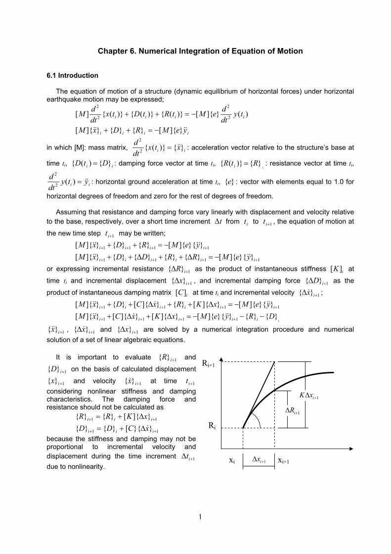
1

Chapter 6. Numerical Integration of Equation of Motion 6.1 Introduction

The equation of motion of a structure (dynamic equilibrium of horizontal forces) under horizontal earthquake motion may be expressed;

iiii

iiii

yeMRDxM

tydtdeMtRtDtx

dtdM

&&&& }]{[}{}{}]{[

)(}]{[)}({)}({)}({][ 2

2

2

2

−=++

−=++

in which [M]: mass matrix, ii xtxdtd }{)}({2

2

&&= : acceleration vector relative to the structure’s base at

time ti, ii DtD }{)({ = : damping force vector at time ti, i

RtR i }{)}({ = : resistance vector at time ti,

ii ytydtd

&&=)(2

2

: horizontal ground acceleration at time ti, }{e : vector with elements equal to 1.0 for

horizontal degrees of freedom and zero for the rest of degrees of freedom.

Assuming that resistance and damping force vary linearly with displacement and velocity relative to the base, respectively, over a short time increment t∆ from it to 1+it , the equation of motion at

the new time step 1+it may be written;

1 1 1 1

1 1 1 1

[ ]{ } { } { } [ ]{ }{ }[ ]{ } { } { } { } { } [ ]{ }{ }

i i i i

i i i i i i

M x D R M e yM x D D R R M e y

+ + + +

+ + + +

+ + = −+ + ∆ + + ∆ = −

&& &&

&& &&

or expressing incremental resistance 1{ }iR +∆ as the product of instantaneous stiffness [ ]iK at

time ti and incremental displacement 1{ }ix +∆ , and incremental damping force 1{ }iD +∆ as the

product of instantaneous damping matrix [ ]iC at time ti and incremental velocity 1{ }ix +∆& ;

1 1 1 1

1 1 1 1

[ ]{ } { } [ ]{ } { } [ ]{ } [ ]{ }{ }[ ]{ } [ ]{ } [ ]{ } [ ]{ }{ } { } { }

i

i i i i i i

i i i i i

M x D C x R K x M e yM x C x K x M e y R D

+ + + +

+ + + +

+ + ∆ + + ∆ = −+ ∆ + ∆ = − − −

&& & &&

&& & &&

1}{ +ix&& , 1}{ +∆ ix& and 1}{ +∆ ix are solved by a numerical integration procedure and numerical solution of a set of linear algebraic equations.

It is important to evaluate 1}{ +iR and

1}{ +iD on the basis of calculated displacement

1}{ +ix and velocity 1}{ +ix& at time 1+it considering nonlinear stiffness and damping characteristics. The damping force and resistance should not be calculated as

11

11

}}{[}{}{}]{[}{}{

++

++

∆+=∆+=

iii

iii

xCDDxKRR&

because the stiffness and damping may not be proportional to incremental velocity and displacement during the time increment 1+∆ it due to nonlinearity.

xi xi+1

Ri

Ri+1

1iR +∆

1iK x +∆

1ix +∆

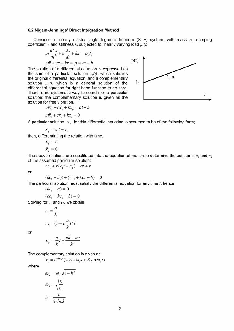
2

6.2 Nigam-Jennings' Direct Integration Method

Consider a linearly elastic single-degree-of-freedom (SDF) system, with mass m, damping coefficient c and stiffness k, subjected to linearly varying load p(t):

batpkxxcxm

tpkxdtdxc

dtxdm

+==++

=++

&&&

)(2

2

The solution of a differential equation is expressed as the sum of a particular solution xp(t), which satisfies the original differential equation, and a complementary solution xc(t), which is a general solution of the differential equation for right hand function to be zero. There is no systematic way to search for a particular solution; the complementary solution is given as the solution for free vibration.

0

p p p

c c c

mx cx kx at b

mx cx kx

+ + = +

+ + =

&& &

&& &

A particular solution px for this differential equation is assumed to be of the following form;

21 ctcxp += then, differentiating the relation with time,

0

1

=

=

p

p

xcx

&&

&

The above relations are substituted into the equation of motion to determine the constants c1 and c2 of the assumed particular solution: batctckcc +=++ )( 211 or 0)()( 211 =−++− bkccctakc The particular solution must satisfy the differential equation for any time t; hence

0)(

0)(

21

1

=−+=−

bkcccakc

Solving for c1 and c2, we obtain

k

kacbc

kac

/)(2

1

−=

=

or

2kacbkt

kaxp

−+=

The complementary solution is given as ( cos sin )nh t

c d dx e A t B tω ω ω−= + where

mkch

mk

h

n

nd

2

1 2

=

=

−=

ω

ωω

t

p(t)

a b

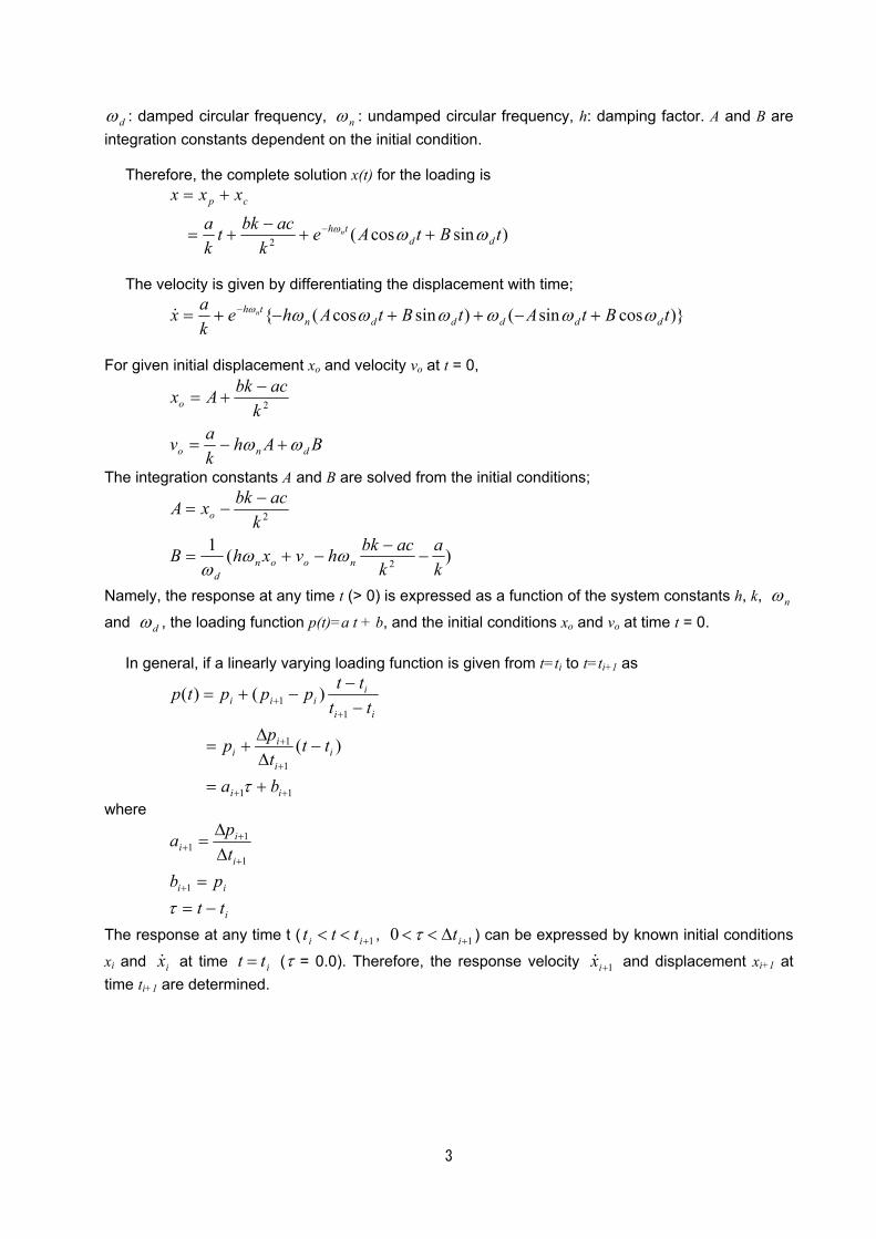
3

dω : damped circular frequency, nω : undamped circular frequency, h: damping factor. A and B are integration constants dependent on the initial condition.

Therefore, the complete solution x(t) for the loading is

)sincos(2 tBtAe

kacbkt

ka

xxx

ddth

cp

n ωωω ++−

+=

+=

−

The velocity is given by differentiating the displacement with time;

)}cossin()sincos({ tBtAtBtAhekax dddddn

th n ωωωωωωω +−++−+= −&

For given initial displacement xo and velocity vo at t = 0,

BAh

kav

kacbkAx

dno

o

ωω +−=

−+= 2

The integration constants A and B are solved from the initial conditions;

)(1

2

2

ka

kacbkhvxhB

kacbkxA

noond

o

−−

−+=

−−=

ωωω

Namely, the response at any time t (> 0) is expressed as a function of the system constants h, k, nω

and dω , the loading function p(t)=a t + b, and the initial conditions xo and vo at time t = 0.

In general, if a linearly varying loading function is given from t=ti to t=ti+1 as

11

1

1

11

)(

)()(

++

+

+

++

+=

−∆∆

+=

−−

−+=

ii

ii

ii

ii

iiii

ba

tttpp

ttttppptp

τ

where

i

ii

i

ii

ttpb

tpa

−==∆∆

=

+

+

++

τ1

1

11

The response at any time t ( 1+<< ii ttt , 10 +∆<< itτ ) can be expressed by known initial conditions

xi and ix& at time itt = (τ = 0.0). Therefore, the response velocity 1+ix& and displacement xi+1 at time ti+1 are determined.

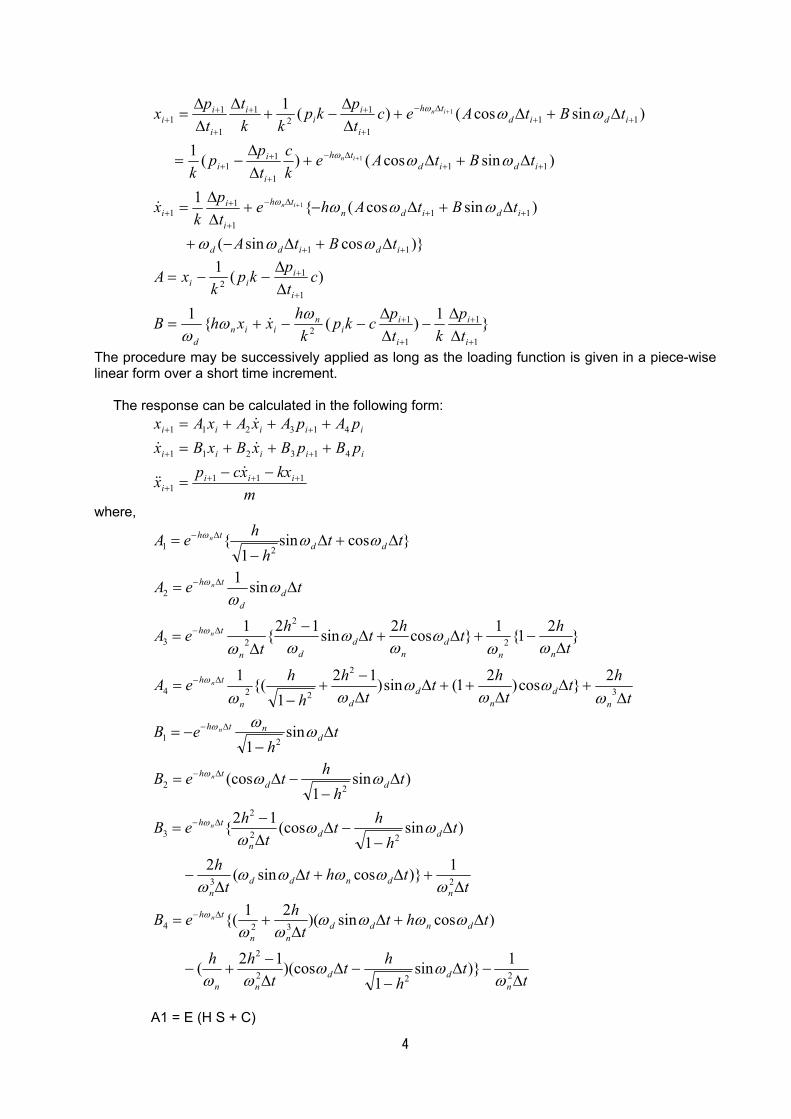
4

)}cossin(

)sincos({1

)sincos()(1

)sincos()(1

11

111

11

111

11

111

12

1

1

11

1

1

1

++

++∆−

+

++

++∆−

+

++

++∆−

+

++

+

++

∆+∆−+

∆+∆−+∆∆

=

∆+∆+∆∆

−=

∆+∆+∆∆

−+∆

∆∆

=

+

+

+

ididd

ididnth

i

ii

ididth

i

ii

ididth

i

ii

i

i

ii

tBtA

tBtAhetp

kx

tBtAekc

tpp

k

tBtAectpkp

kkt

tpx

in

in

in

ωωω

ωωω

ωω

ωω

ω

ω

ω

&

}1)({1

)(1

1

1

1

12

1

12

+

+

+

+

+

+

∆∆

−∆∆

−−+=

∆∆

−−=

i

i

i

ii

niin

d

i

iii

tp

ktpckp

khxxhB

ctpkp

kxA

ωωω

&

The procedure may be successively applied as long as the loading function is given in a piece-wise linear form over a short time increment.

The response can be calculated in the following form:

mkxxcpx

pBpBxBxBxpApAxAxAx

iiii

iiiii

iiiii

1111

413211

413211

++++

++

++

−−=

+++=+++=

&&&

&&

&

where,

tht

tht

th

hheA

ththth

teA

teA

tth

heA

nd

nd

dn

th

nnd

nd

dn

th

dd

th

ddth

n

n

n

n

∆+∆

∆++∆

∆−

+−

=

∆−+∆+∆

−∆

=

∆=

∆+∆−

=

∆−

∆−

∆−

∆−

3

2

224

2

2

23

2

21

2}cos)21(sin)121

{(1

}21{1}cos2sin12{1

sin1

}cossin1

{

ωω

ωω

ωω

ωωω

ωω

ωω

ωω

ωω

ω

ω

ω

ω

ttht

th

th

htt

heB

th

hteB

th

eB

ndndd

n

ddn

th

ddth

dnth

n

n

n

∆+∆+∆

∆−

∆−

−∆∆−

=

∆−

−∆=

∆−

−=

∆−

∆−

∆−

23

22

2

3

22

21

1)}cossin(2

)sin1

(cos12{

)sin1

(cos

sin1

ωωωωω

ω

ωωω

ωω

ωω

ω

ω

ω

tt

hht

thh

thtt

heB

ndd

nn

dnddnn

th n

∆−∆

−−∆

∆−

+−

∆+∆∆

+= ∆−

222

2

324

1)}sin1

)(cos12(

)cossin)(21{(

ωωω

ωω

ωωωωωω

ω

A1 = E (H S + C)

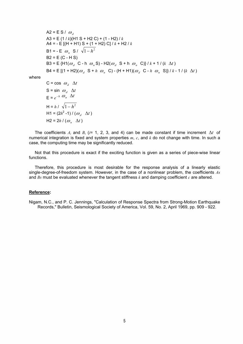
5

A2 = E S / dω A3 = E (1 / k)(H1 S + H2 C) + (1 - H2) / k A4 = - E [(H + H1) S + (1 + H2) C] / k + H2 / k

B1 = - E nω S / 21 h− B2 = E (C - H S) B3 = E {H1( dω C - h nω S) - H2( dω S + h nω C)} / k + 1 / (k t∆ )

B4 = E [(1 + H2)( dω S + h nω C) - (H + H1)( dω C - h nω S)} / k - 1 / (k t∆ ) where C = cos dω t∆

S = sin dω t∆

E = e - h nω t∆

H = h / 21 h− H1 = (2h2 -1) / ( dω t∆ )

H2 = 2h / ( nω t∆ )

The coefficients Ai and Bi (i= 1, 2, 3, and 4) can be made constant if time increment t∆ of numerical integration is fixed and system properties m, c, and k do not change with time. In such a case, the computing time may be significantly reduced.

Not that this procedure is exact if the exciting function is given as a series of piece-wise linear functions.

Therefore, this procedure is most desirable for the response analysis of a linearly elastic single-degree-of-freedom system. However, in the case of a nonlinear problem, the coefficients As and Bs must be evaluated whenever the tangent stiffness k and damping coefficient c are altered. Reference: Nigam, N.C., and P. C. Jennings, "Calculation of Response Spectra from Strong-Motion Earthquake

Records," Bulletin, Seismological Society of America, Vol. 59, No. 2, April 1969, pp. 909 - 922.

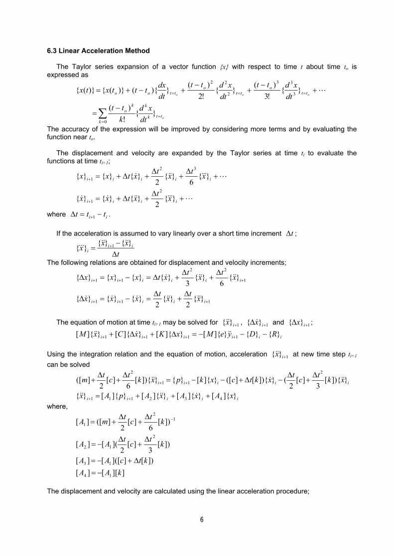
6

6.3 Linear Acceleration Method

The Taylor series expansion of a vector function {x} with respect to time t about time to is expressed as

o

ooo

ttk

k

k

ko

tto

tto

ttoo

dtxd

ktt

dtxdtt

dtxdtt

dtdxtttxtx

==

===

∑ −=

+−

+−

+−+=

}{!

)(

}{!3

)(}{

!2)(

}){()}({)}({

0

3

33

2

22

L

The accuracy of the expression will be improved by considering more terms and by evaluating the function near to.

The displacement and velocity are expanded by the Taylor series at time ti to evaluate the functions at time ti+1;

L&&&&&&&

L&&&&&&

+∆

+∆+=

+∆

+∆

+∆+=

+

+

iiii

iiiii

xtxtxx

xtxtxtxx

}{2

}{}{}{

}{6

}{2

}{}{}{

2

1

32

1

where ii ttt −=∆ +1 .

If the acceleration is assumed to vary linearly over a short time increment t∆ ;

1{ } { }{ } i ii

x xxt

+ −=

∆&& &&

&&&

The following relations are obtained for displacement and velocity increments;

111

1

22

11

}{2

}{2

}{}{}{

}{6

}{3

}{}{}{}{

+++

+++

∆+

∆=−=∆

∆+

∆+∆=−=∆

iiiii

iiiiii

xtxtxxx

xtxtxtxxx

&&&&&&&

&&&&&

The equation of motion at time ti+1 may be solved for 1}{ +ix&& , 1}{ +∆ ix& and 1}{ +∆ ix ;

iiiiii RDyeMxKxCxM }{}{}]{[}]{[}]{[}]{[ 1111 −−−=∆+∆+ ++++ &&&&& Using the integration relation and the equation of motion, acceleration 1{ }ix +&& at new time step ti+1 can be solved

2 2

1 1([ ] [ ] [ ]){ } { } [ ]{ } ([ ] [ ]){ } ( [ ] [ ]){ }2 6 2 3i i i i it t t tm c k x p k x c t k x c k x+ +

∆ ∆ ∆ ∆+ + = − − + ∆ − +&& & &&

iiiii xAxAxApAx }]{[}]{[}]{[}]{[}{ 432111 +++= ++ &&&&& where,

]][[][])[]]([[][

])[3

][2

]([][

])[6

][2

]([][

14

13

2

12

12

1

kAAktcAA

ktctAA

ktctmA

−=∆+−=

∆+

∆−=

∆+

∆+= −

The displacement and velocity are calculated using the linear acceleration procedure;

7

11

122

1

}{21}{

21}{}{

}{61}{

31}{}{}{

++

++

∆+∆+=

∆+∆+∆+=

iiii

iiiii

xtxtxx

xtxtxtxx

&&&&&&

&&&&&

The time increment t∆ for the response analysis must be chosen to satisfy the following

conditions; (a) Excitation function, hysteresis relations, and response waveforms can be expressed

with a satisfactory accuracy, (b) The accuracy of response results can be attained, and (c) The numerical integration gives stable results.

The solution of the linear acceleration method diverges if the time increment is selected larger than 1/3 of the shortest modal period of oscillation of the system.

8

6.4 Newmark Beta Method

For a set of differential equation of motion given below, iiiiii RDyeMxKxCxM }{}{}]{[}]{[}]{[}]{[ 1111 −−−=∆+∆+ ++++ &&&&& Newmark (1959) suggested the following relations for the numerical integration;

111

122

11

}{}{)1(}{}{}{

}{}{)21(}{}{}{}{

+++

+++

∆+∆−=−=∆

∆+∆−+∆=−=∆

iiiii

iiiiii

xtxtxxx

xtxtxtxxx

&&&&&&&

&&&&&

γγ

ββ

where β and γ are constants of the Newmark Beta method. The value of γ must be 1/2, and 1/ 4β ≤ . If the value of γ is selected to be greater than 1/2, the response amplitude becomes greater than the true value; if the value is smaller than 1/2, then the amplitude becomes smaller. For the numerical integration to give stable results, the time increment t∆ must be less than one-sixth of the shortest modal period of the system for β = 1/6. The scheme is known to be unconditionally stable for β = 1/4.

The equation motion can be solved for the acceleration 1}{ +ix&& at the new time step;

iiiiii

i

xKtxKtxCtRDp

xKtCtM

}]{[)21(}]{[}]{[)1(}{}{}{

}]){[][]{[

21

12

&&&&&

&&

∆−−∆−∆−−−−=

∆+∆+

+

+

βγ

βγ

Newmark suggested to solve the set of equations by an iteration method; (a) Assume acceleration vector *

1}{ +ix&& at time ti+1,

(b) Evaluate the displacement increment *1}{ +∆ ix and velocity increment *

1}{ +∆ ix& by the following relations;

*1

*1

*1

*1

*1

*1

*1

22*1

}{}{}{

}{}{}{

}{}{)1(}{

}{}{)21(}{}{

++

++

++

++

∆+=

∆+=

∆+∆−=∆

∆+∆−+∆=∆

iii

iii

iii

iiii

xxx

xxx

xtxtx

xtxtxtx

&&&

&&&&&

&&&&&

γγ

ββ

(c) Evaluate damping force {D}*i+1 and resistance {R}*i+1 for the calculated velocity *1}{ +ix&

and displacement *1}{ +ix on the basis of damping and hysteresis models;

(d) Re-evaluate the acceleration 1}{ +ix&& by the equation of motion at time ti+1;

1111 }{}{}]{[}]{[ ++++ −−−= iiii RDyeMxM &&&&

(e) If the re-evaluated acceleration 1}{ +ix&& differs from the assumed acceleration *1}{ +ix&& by

more than a specified tolerance }{ε , the assumed acceleration *1}{ +ix&& is replaced by the

re-evaluated acceleration 1}{ +ix&& in step (a), and the procedure is iterated until a satisfactory conversion is achieved.

Sharpe and Carr (1974) studied a condition for numerical stability as follows;

1.0derived acceleration true accelerationassumed acceleration true acceleration

−≤

−

at the end of each time step using Newmark Beta scheme. They derived a convergence criteria as

9

follows;

21 1[ ( ) ]2 2 2

t h hT π β β β∆

< − + +

Newmark (1959) showed the convergence criteria for an undamped linear system as follows;

1 1

2t

T π β∆

≤

For 16

β = equivalent to the linear acceleration scheme,

0.39tT∆

≤

Sharpe and Carr (1974) extended Newmark’s derivation of convergence for undamped system to

damped system. The criterion is shown below;

21

1 4t h

T π β∆ −

<−

References Newmark, N. M., "A Method of Computation for Structural Dynamics," Journal, Engineering

Mechanics Division, ASCE, July 1959, pp. 67 - 94. Sharpe, R. D., and A. J. Carr, "The Seismic Response of Inelastic Structures," Research Report

74-13, Department of Civil Engineering, University of Canterbury, New Zealand, November 1974.

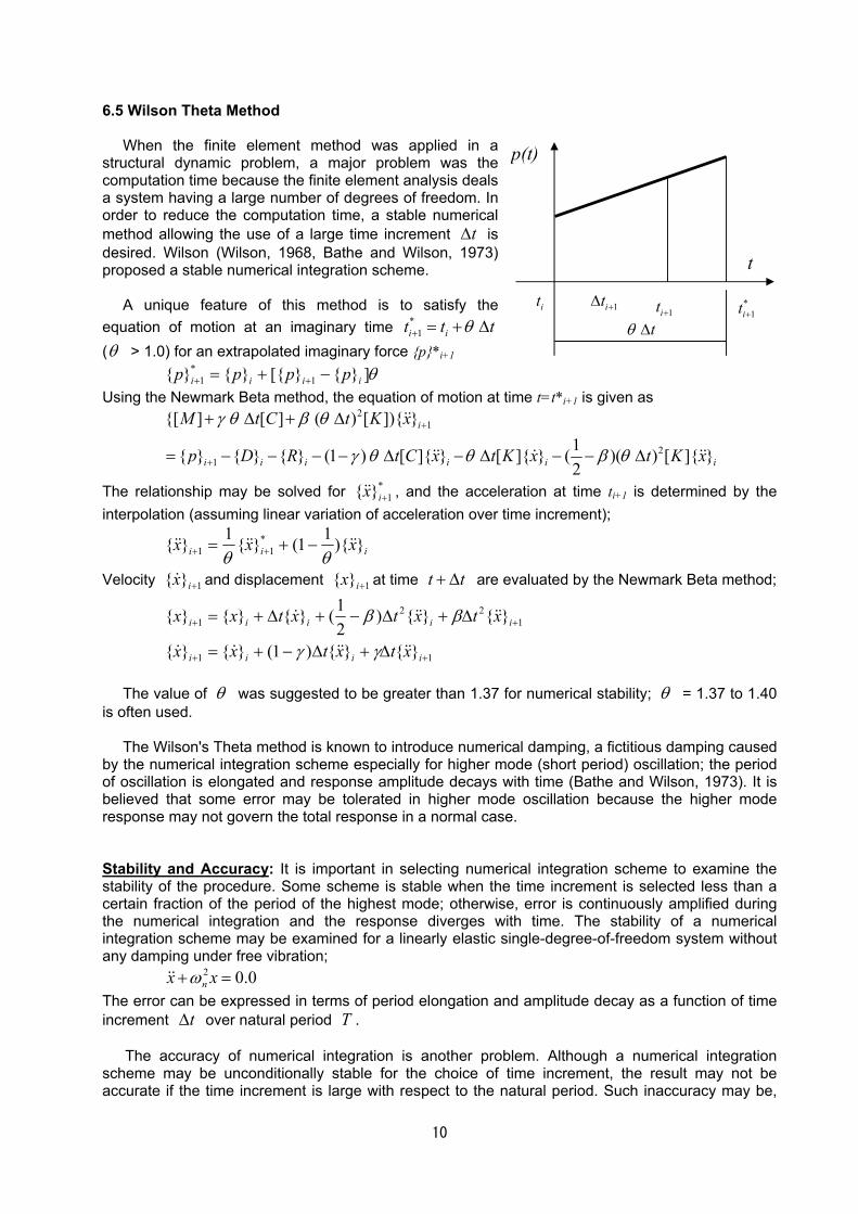
10

6.5 Wilson Theta Method

When the finite element method was applied in a structural dynamic problem, a major problem was the computation time because the finite element analysis deals a system having a large number of degrees of freedom. In order to reduce the computation time, a stable numerical method allowing the use of a large time increment t∆ is desired. Wilson (Wilson, 1968, Bathe and Wilson, 1973) proposed a stable numerical integration scheme.

A unique feature of this method is to satisfy the equation of motion at an imaginary time *

1i it t tθ+ = + ∆ (θ > 1.0) for an extrapolated imaginary force {p}*i+1 θ]}{}[{}{}{ 1

*1 iiii pppp −+= ++

Using the Newmark Beta method, the equation of motion at time t=t*i+1 is given as

21

21

{[ ] [ ] ( ) [ ]){ }1{ } { } { } (1 ) [ ]{ } [ ]{ } ( )( ) [ ]{ }2

i

i i i i i i

M t C t K x

p D R t C x t K x t K x

γ θ β θ

γ θ θ β θ

+

+

+ ∆ + ∆

= − − − − ∆ − ∆ − − ∆

&&

&& & &&

The relationship may be solved for *1}{ +ix&& , and the acceleration at time ti+1 is determined by the

interpolation (assuming linear variation of acceleration over time increment);

iii xxx }){11(}{1}{ *11 &&&&&&

θθ−+= ++

Velocity 1}{ +ix& and displacement 1}{ +ix at time t t+ ∆ are evaluated by the Newmark Beta method;

11

122

1

}{}{)1(}{}{

}{}{)21(}{}{}{

++

++

∆+∆−+=

∆+∆−+∆+=

iiii

iiiii

xtxtxx

xtxtxtxx

&&&&&&

&&&&&

γγ

ββ

The value of θ was suggested to be greater than 1.37 for numerical stability; θ = 1.37 to 1.40

is often used.

The Wilson's Theta method is known to introduce numerical damping, a fictitious damping caused by the numerical integration scheme especially for higher mode (short period) oscillation; the period of oscillation is elongated and response amplitude decays with time (Bathe and Wilson, 1973). It is believed that some error may be tolerated in higher mode oscillation because the higher mode response may not govern the total response in a normal case. Stability and Accuracy: It is important in selecting numerical integration scheme to examine the stability of the procedure. Some scheme is stable when the time increment is selected less than a certain fraction of the period of the highest mode; otherwise, error is continuously amplified during the numerical integration and the response diverges with time. The stability of a numerical integration scheme may be examined for a linearly elastic single-degree-of-freedom system without any damping under free vibration;

2 0.0nx xω+ =&& The error can be expressed in terms of period elongation and amplitude decay as a function of time increment t∆ over natural period T .

The accuracy of numerical integration is another problem. Although a numerical integration scheme may be unconditionally stable for the choice of time increment, the result may not be accurate if the time increment is large with respect to the natural period. Such inaccuracy may be,

it 1it + tθ ∆

1it +∆ *1it +

t

p(t)

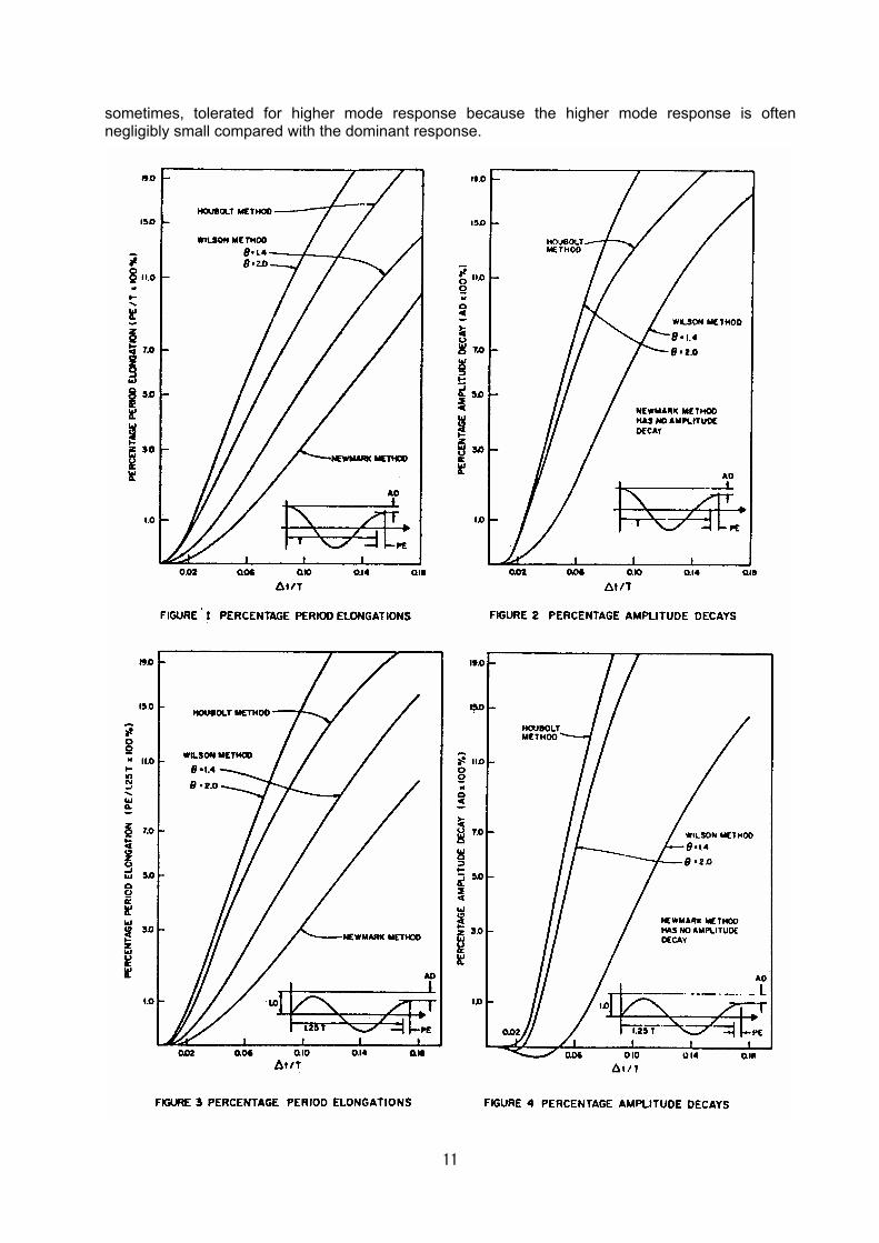
11

sometimes, tolerated for higher mode response because the higher mode response is often negligibly small compared with the dominant response.

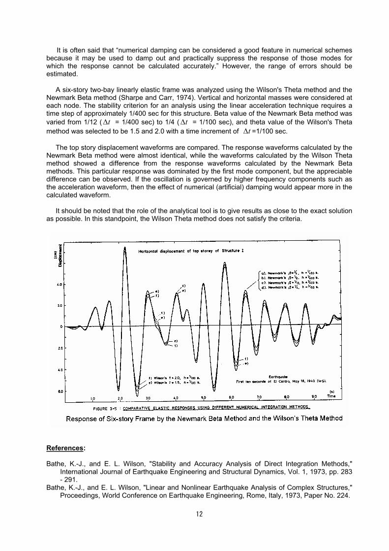
12

It is often said that “numerical damping can be considered a good feature in numerical schemes because it may be used to damp out and practically suppress the response of those modes for which the response cannot be calculated accurately.” However, the range of errors should be estimated.

A six-story two-bay linearly elastic frame was analyzed using the Wilson's Theta method and the

Newmark Beta method (Sharpe and Carr, 1974). Vertical and horizontal masses were considered at each node. The stability criterion for an analysis using the linear acceleration technique requires a time step of approximately 1/400 sec for this structure. Beta value of the Newmark Beta method was varied from 1/12 ( t∆ = 1/400 sec) to 1/4 ( t∆ = 1/100 sec), and theta value of the Wilson's Theta method was selected to be 1.5 and 2.0 with a time increment of t∆ =1/100 sec.

The top story displacement waveforms are compared. The response waveforms calculated by the Newmark Beta method were almost identical, while the waveforms calculated by the Wilson Theta method showed a difference from the response waveforms calculated by the Newmark Beta methods. This particular response was dominated by the first mode component, but the appreciable difference can be observed. If the oscillation is governed by higher frequency components such as the acceleration waveform, then the effect of numerical (artificial) damping would appear more in the calculated waveform.

It should be noted that the role of the analytical tool is to give results as close to the exact solution as possible. In this standpoint, the Wilson Theta method does not satisfy the criteria.

References: Bathe, K.-J., and E. L. Wilson, "Stability and Accuracy Analysis of Direct Integration Methods,"

International Journal of Earthquake Engineering and Structural Dynamics, Vol. 1, 1973, pp. 283 - 291.

Bathe, K.-J., and E. L. Wilson, "Linear and Nonlinear Earthquake Analysis of Complex Structures," Proceedings, World Conference on Earthquake Engineering, Rome, Italy, 1973, Paper No. 224.

13

Hilber, H.M., et al., “Improved Numerical Dissipation for Time Integration Algorithms in Structural Dynamics,” Earthquake Engineering & Structural Dynamics, No. 5, 1977, pp. 283 - 292.

Sharpe, R. D., and A. J. Carr, "The Seismic Response of Inelastic Structures," Research Report 74-13, Department of Civil Engineering, University of Canterbury, New Zealand, November 1974.

Wilson, E. L., "A Computer Program for the Dynamic Stress Analysis of Underground Structures," SESM Report 68-1, Department of Civil Engineering, University of California, Berkeley, 1968.

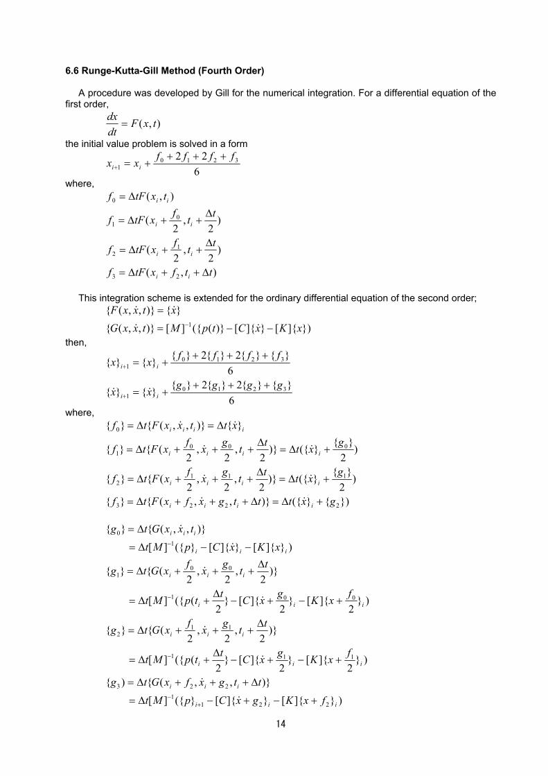
14

6.6 Runge-Kutta-Gill Method (Fourth Order)

A procedure was developed by Gill for the numerical integration. For a differential equation of the first order,

),( txFdtdx

=

the initial value problem is solved in a form

6

22 32101

ffffxx ii+++

+=+

where,

),(

)2

,2

(

)2

,2

(

),(

23

12

01

0

ttfxtFf

ttfxtFf

ttfxtFf

txtFf

ii

ii

ii

ii

∆++∆=

∆++∆=

∆++∆=

∆=

This integration scheme is extended for the ordinary differential equation of the second order;

})]{[}]{[)}(({][)},,({

}{)},,({1 xKxCtpMtxxG

xtxxF−−=

=− &&

&&

then,

6}{}{2}{2}{}{}{

6}{}{2}{2}{}{}{

32101

32101

ggggxx

ffffxx

ii

ii

++++=

++++=

+

+

&&

where,

}){}({)},,({}{

)2

}{}({)}2

,2

,2

({}{

)2

}{}({)}2

,2

,2

({}{

}{)},,({}{

2223

1112

0001

0

gxtttgxfxFtf

gxtttgxfxFtf

gxtttgxfxFtf

xttxxFtf

iiii

iiii

iiii

iiii

+∆=∆+++∆=

+∆=∆

+++∆=

+∆=∆

+++∆=

∆=∆=

&&

&&

&&

&&

)}]{[}]{[}({][

)},,({){

)}2

]{[}2

]{[}2

(({][

)}2

,2

,2

({}{

)}2

]{[}2

]{[}2

(({][

)}2

,2

,2

({}{

)}]{[}]{[}({][

)},,({}{

2211

223

111

112

001

001

10

iii

iii

iii

iii

iii

iii

iii

iii

fxKgxCpMt

ttgxfxGtg

fxKgxCttpMt

ttgxfxGtg

fxKgxCttpMt

ttgxfxGtg

xKxCpMt

txxGtg

+−+−∆=

∆+++∆=

+−+−∆

+∆=

∆+++∆=

+−+−∆

+∆=

∆+++∆=

−−∆=

∆=

+−

−

−

−

&

&

&

&

&

&

&

&

15

Reference: Gill, S., "A Procedure for the Step-by-step Integration of Differential Equations in an Automatic

Computing Machine," Proceedings, Cambridge Philosophical Society, 49:96, 1951.

16

Appendix: Linearly elastic response of SDF System under earthquake motion (FORTRAN） C C RESPONSE OF A SINGLE-DEGREE-OF-FREEDOM LINEARLY ELASTIC SYSTEM C TO EARTHQUAKE MOTION C C PROGRAMMED BY OTANI, S. C ON OCTOBER 28, 1975 C AT UNIVERSITY OF TORONTO C MODIFIED BY OTANI, S. C ON APRIL 18, 1993 C AT UNIVERSITY OF TOKYO C MODIFIED BY OTANI, S. C ON MAY 26, 2000 C AT UNIVERSITY OF TOKYO C C THE EQUATION OF MOTION OF SDF SYSTEM UNDER GROUND MOTION C C DDX + 2.0 * BT * WN * DX + WN * WN * X = - DDY C C INPUT DATA C 1. TITL C TITL: TITLE OF STUDY C 2. LUNT,TUNT C LUNT: UNIT OF LENGTH C TUNT: UNIT OF TIME C 3. TN,BT,DT,ASCL,V0,D0 C TN: PERIOD C BT: DAMPING RATIO C DT: TIME INTERVAL OF NUMERICAL INTEGRATION C ASC: SCALE FACTOR FOR GROUND ACCELERATION C V0: INITIAL VELOCITY C D0: INITIAL DISPLACEMENT C 4. NSTT,NSTP,MTHD C NSTT: STARTING POINT OF EARTHQUAKE DATA C NSTP: TERMINATING POINT OF EARTHQUAKE DATA C MTHD: POINTER FOR NUMBERICAL INTEGRATION METHOD C 5. EQNM C EQNM: NAME OF EARTHQUAKE RECORD C 6. TIME,GACC C TIME: TIME COORDINATE OF EARTHQUAKE DATA C GACC: GROUND ACCELERATION OF EARTHQUAKE DATA C CHARACTER*4 TITLE(18)*4,EQNM(18)*4,LUNT*4,TUNT*4 DIMENSION TIME(2),GACC(2) C READ (5,500) TITL READ (5,500) LUNT,TUNT C READ (5,*) TN,BT,DT,ASCL,V0,D0 C TN UNDAMPED NATURAL PERIOD IF (TN.LE.0.0) GO TO 60 C BT DAMPING FACTOR IF (BT.LT.0.0) BT=0.0 C DT TIME INCREMENT OF NUMERICAL INTEGRATION IF (DT.LE.0.0) DT=0.05*TN C ASCL SCALE FACTOR FOR GROUND ACCELERATION DATA IF (ASCL.LE.0.0) ASCL=1.0 C FN UNDAMPED NATURAL FREQUENCY FN=1.0/TN WN=6.2830*FN BW=2.0*BT*WN W2=WN*WN C PRINT INPUT INFORMATION WRITE (6,600) TITL,LUNT,TUNT WRITE (6,602) TN,TUNT,FN,TUNT,WN,TUNT,BT,DT,TUNT,ASCL, 1 V0,LUNT,TUNT,D0,LUNT

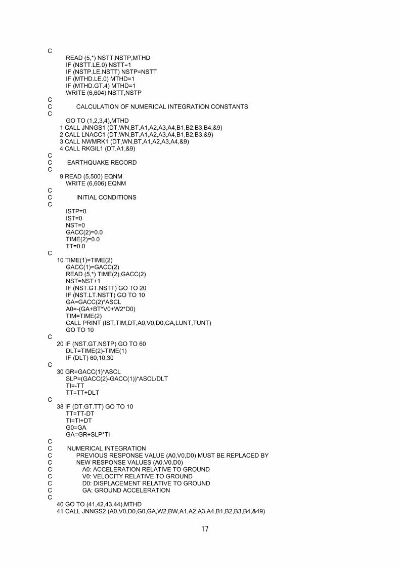
17

C READ (5,*) NSTT,NSTP,MTHD IF (NSTT.LE.0) NSTT=1 IF (NSTP.LE.NSTT) NSTP=NSTT IF (MTHD.LE.0) MTHD=1 IF (MTHD.GT.4) MTHD=1 WRITE (6,604) NSTT,NSTP C C CALCULATION OF NUMERICAL INTEGRATION CONSTANTS C GO TO (1,2,3,4),MTHD 1 CALL JNNGS1 (DT,WN,BT,A1,A2,A3,A4,B1,B2,B3,B4,&9) 2 CALL LNACC1 (DT,WN,BT,A1,A2,A3,A4,B1,B2,B3,&9) 3 CALL NWMRK1 (DT,WN,BT,A1,A2,A3,A4,&9) 4 CALL RKGIL1 (DT,A1,&9) C C EARTHQUAKE RECORD C 9 READ (5,500) EQNM WRITE (6,606) EQNM C C INITIAL CONDITIONS C ISTP=0 IST=0 NST=0 GACC(2)=0.0 TIME(2)=0.0 TT=0.0 C 10 TIME(1)=TIME(2) GACC(1)=GACC(2) READ (5,*) TIME(2),GACC(2) NST=NST+1 IF (NST.GT.NSTT) GO TO 20 IF (NST.LT.NSTT) GO TO 10 GA=GACC(2)*ASCL A0=-(GA+BT*V0+W2*D0) TIM=TIME(2) CALL PRINT (IST,TIM,DT,A0,V0,D0,GA,LUNT,TUNT) GO TO 10 C 20 IF (NST.GT.NSTP) GO TO 60 DLT=TIME(2)-TIME(1) IF (DLT) 60,10,30 C 30 GR=GACC(1)*ASCL SLP=(GACC(2)-GACC(1))*ASCL/DLT TI=-TT TT=TT+DLT C 38 IF (DT.GT.TT) GO TO 10 TT=TT-DT TI=TI+DT G0=GA GA=GR+SLP*TI C C NUMERICAL INTEGRATION C PREVIOUS RESPONSE VALUE (A0,V0,D0) MUST BE REPLACED BY C NEW RESPONSE VALUES (A0,V0,D0) C A0: ACCELERATION RELATIVE TO GROUND C V0: VELOCITY RELATIVE TO GROUND C D0: DISPLACEMENT RELATIVE TO GROUND C GA: GROUND ACCELERATION C 40 GO TO (41,42,43,44),MTHD 41 CALL JNNGS2 (A0,V0,D0,G0,GA,W2,BW,A1,A2,A3,A4,B1,B2,B3,B4,&49)

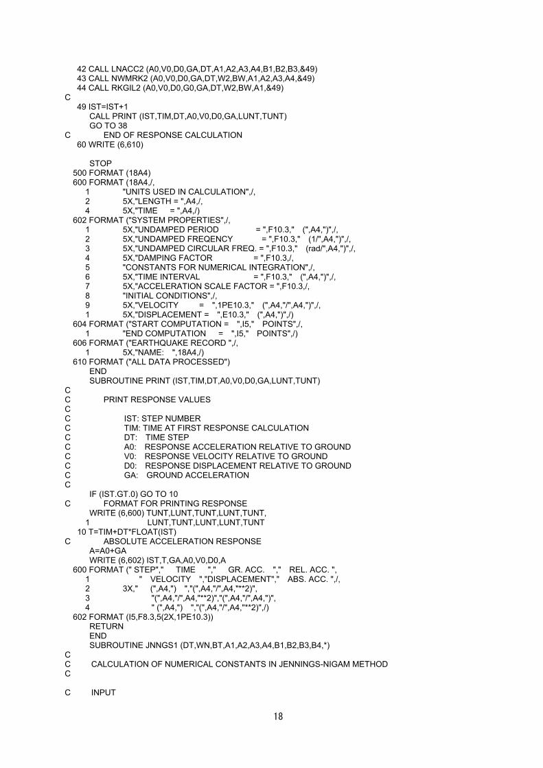
18

42 CALL LNACC2 (A0,V0,D0,GA,DT,A1,A2,A3,A4,B1,B2,B3,&49) 43 CALL NWMRK2 (A0,V0,D0,GA,DT,W2,BW,A1,A2,A3,A4,&49) 44 CALL RKGIL2 (A0,V0,D0,G0,GA,DT,W2,BW,A1,&49) C 49 IST=IST+1 CALL PRINT (IST,TIM,DT,A0,V0,D0,GA,LUNT,TUNT) GO TO 38 C END OF RESPONSE CALCULATION 60 WRITE (6,610) STOP 500 FORMAT (18A4) 600 FORMAT (18A4,/, 1 "UNITS USED IN CALCULATION",/, 2 5X,"LENGTH = ",A4,/, 4 5X,"TIME = ",A4,/) 602 FORMAT ("SYSTEM PROPERTIES",/, 1 5X,"UNDAMPED PERIOD = ",F10.3," (",A4,")",/, 2 5X,"UNDAMPED FREQENCY = ",F10.3," (1/",A4,")",/, 3 5X,"UNDAMPED CIRCULAR FREQ. = ",F10.3," (rad/",A4,")",/, 4 5X,"DAMPING FACTOR = ",F10.3,/, 5 "CONSTANTS FOR NUMERICAL INTEGRATION",/, 6 5X,"TIME INTERVAL = ",F10.3," (",A4,")",/, 7 5X,"ACCELERATION SCALE FACTOR = ",F10.3,/, 8 "INITIAL CONDITIONS",/, 9 5X,"VELOCITY = ",1PE10.3," (",A4,"/",A4,")",/, 1 5X,"DISPLACEMENT = ",E10.3," (",A4,")",/) 604 FORMAT ("START COMPUTATION = ",I5," POINTS",/, 1 "END COMPUTATION = ",I5," POINTS",/) 606 FORMAT ("EARTHQUAKE RECORD ",/, 1 5X,"NAME: ",18A4,/) 610 FORMAT ("ALL DATA PROCESSED") END SUBROUTINE PRINT (IST,TIM,DT,A0,V0,D0,GA,LUNT,TUNT) C C PRINT RESPONSE VALUES C C IST: STEP NUMBER C TIM: TIME AT FIRST RESPONSE CALCULATION C DT: TIME STEP C A0: RESPONSE ACCELERATION RELATIVE TO GROUND C V0: RESPONSE VELOCITY RELATIVE TO GROUND C D0: RESPONSE DISPLACEMENT RELATIVE TO GROUND C GA: GROUND ACCELERATION C IF (IST.GT.0) GO TO 10 C FORMAT FOR PRINTING RESPONSE WRITE (6,600) TUNT,LUNT,TUNT,LUNT,TUNT, 1 LUNT,TUNT,LUNT,LUNT,TUNT 10 T=TIM+DT*FLOAT(IST) C ABSOLUTE ACCELERATION RESPONSE A=A0+GA WRITE (6,602) IST,T,GA,A0,V0,D0,A 600 FORMAT (" STEP"," TIME "," GR. ACC. "," REL. ACC. ", 1 " VELOCITY ","DISPLACEMENT"," ABS. ACC. ",/, 2 3X," (",A4,") ","(",A4,"/",A4,"**2)", 3 "(",A4,"/",A4,"**2)","(",A4,"/",A4,")", 4 " (",A4,") ","(",A4,"/",A4,"**2)",/) 602 FORMAT (I5,F8.3,5(2X,1PE10.3)) RETURN END SUBROUTINE JNNGS1 (DT,WN,BT,A1,A2,A3,A4,B1,B2,B3,B4,*) C C CALCULATION OF NUMERICAL CONSTANTS IN JENNINGS-NIGAM METHOD C C INPUT

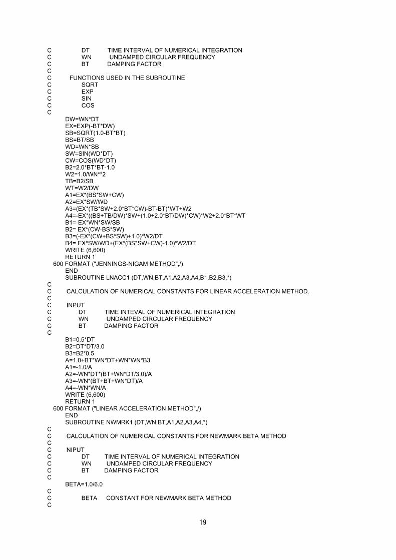
19

C DT TIME INTERVAL OF NUMERICAL INTEGRATION C WN UNDAMPED CIRCULAR FREQUENCY C BT DAMPING FACTOR C C FUNCTIONS USED IN THE SUBROUTINE C SQRT C EXP C SIN C COS C DW=WN*DT EX=EXP(-BT*DW) SB=SQRT(1.0-BT*BT) BS=BT/SB WD=WN*SB SW=SIN(WD*DT) CW=COS(WD*DT) B2=2.0*BT*BT-1.0 W2=1.0/WN**2 TB=B2/SB WT=W2/DW A1=EX*(BS*SW+CW) A2=EX*SW/WD A3=(EX*(TB*SW+2.0*BT*CW)-BT-BT)*WT+W2 A4=-EX*((BS+TB/DW)*SW+(1.0+2.0*BT/DW)*CW)*W2+2.0*BT*WT B1=-EX*WN*SW/SB B2= EX*(CW-BS*SW) B3=(-EX*(CW+BS*SW)+1.0)*W2/DT B4= EX*SW/WD+(EX*(BS*SW+CW)-1.0)*W2/DT WRITE (6,600) RETURN 1 600 FORMAT ("JENNINGS-NIGAM METHOD",/) END SUBROUTINE LNACC1 (DT,WN,BT,A1,A2,A3,A4,B1,B2,B3,*) C C CALCULATION OF NUMERICAL CONSTANTS FOR LINEAR ACCELERATION METHOD. C C INPUT C DT TIME INTEVAL OF NUMERICAL INTEGRATION C WN UNDAMPED CIRCULAR FREQUENCY C BT DAMPING FACTOR C B1=0.5*DT B2=DT*DT/3.0 B3=B2*0.5 A=1.0+BT*WN*DT+WN*WN*B3 A1=-1.0/A A2=-WN*DT*(BT+WN*DT/3.0)/A A3=-WN*(BT+BT+WN*DT)/A A4=-WN*WN/A WRITE (6,600) RETURN 1 600 FORMAT ("LINEAR ACCELERATION METHOD",/) END SUBROUTINE NWMRK1 (DT,WN,BT,A1,A2,A3,A4,*) C C CALCULATION OF NUMERICAL CONSTANTS FOR NEWMARK BETA METHOD C C NIPUT C DT TIME INTERVAL OF NUMERICAL INTEGRATION C WN UNDAMPED CIRCULAR FREQUENCY C BT DAMPING FACTOR C BETA=1.0/6.0 C C BETA CONSTANT FOR NEWMARK BETA METHOD C

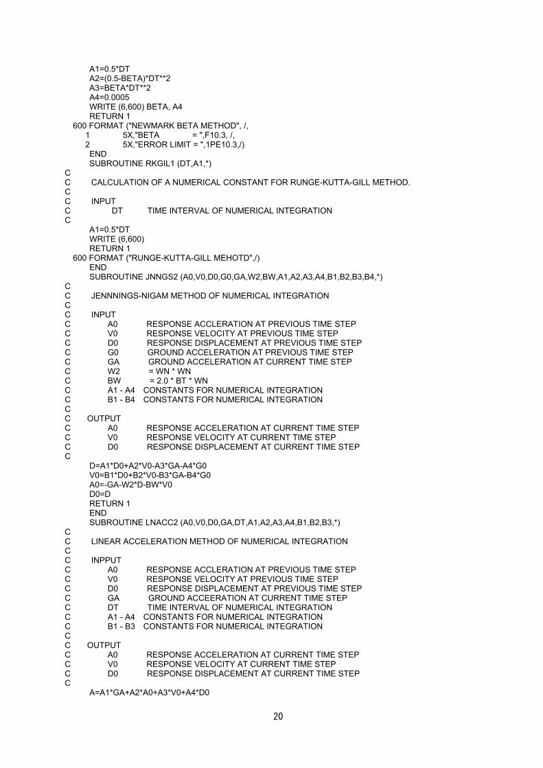
20

A1=0.5*DT A2=(0.5-BETA)*DT**2 A3=BETA*DT**2 A4=0.0005 WRITE (6,600) BETA, A4 RETURN 1 600 FORMAT ("NEWMARK BETA METHOD", /, 1 5X,"BETA = ",F10.3, /, 2 5X,"ERROR LIMIT = ",1PE10.3,/) END SUBROUTINE RKGIL1 (DT,A1,*) C C CALCULATION OF A NUMERICAL CONSTANT FOR RUNGE-KUTTA-GILL METHOD. C C INPUT C DT TIME INTERVAL OF NUMERICAL INTEGRATION C A1=0.5*DT WRITE (6,600) RETURN 1 600 FORMAT ("RUNGE-KUTTA-GILL MEHOTD",/) END SUBROUTINE JNNGS2 (A0,V0,D0,G0,GA,W2,BW,A1,A2,A3,A4,B1,B2,B3,B4,*) C C JENNNINGS-NIGAM METHOD OF NUMERICAL INTEGRATION C C INPUT C A0 RESPONSE ACCLERATION AT PREVIOUS TIME STEP C V0 RESPONSE VELOCITY AT PREVIOUS TIME STEP C D0 RESPONSE DISPLACEMENT AT PREVIOUS TIME STEP C G0 GROUND ACCELERATION AT PREVIOUS TIME STEP C GA GROUND ACCELERATION AT CURRENT TIME STEP C W2 = WN * WN C BW = 2.0 * BT * WN C A1 - A4 CONSTANTS FOR NUMERICAL INTEGRATION C B1 - B4 CONSTANTS FOR NUMERICAL INTEGRATION C C OUTPUT C A0 RESPONSE ACCELERATION AT CURRENT TIME STEP C V0 RESPONSE VELOCITY AT CURRENT TIME STEP C D0 RESPONSE DISPLACEMENT AT CURRENT TIME STEP C D=A1*D0+A2*V0-A3*GA-A4*G0 V0=B1*D0+B2*V0-B3*GA-B4*G0 A0=-GA-W2*D-BW*V0 D0=D RETURN 1 END SUBROUTINE LNACC2 (A0,V0,D0,GA,DT,A1,A2,A3,A4,B1,B2,B3,*) C C LINEAR ACCELERATION METHOD OF NUMERICAL INTEGRATION C C INPPUT C A0 RESPONSE ACCLERATION AT PREVIOUS TIME STEP C V0 RESPONSE VELOCITY AT PREVIOUS TIME STEP C D0 RESPONSE DISPLACEMENT AT PREVIOUS TIME STEP C GA GROUND ACCEERATION AT CURRENT TIME STEP C DT TIME INTERVAL OF NUMERICAL INTEGRATION C A1 - A4 CONSTANTS FOR NUMERICAL INTEGRATION C B1 - B3 CONSTANTS FOR NUMERICAL INTEGRATION C C OUTPUT C A0 RESPONSE ACCELERATION AT CURRENT TIME STEP C V0 RESPONSE VELOCITY AT CURRENT TIME STEP C D0 RESPONSE DISPLACEMENT AT CURRENT TIME STEP C A=A1*GA+A2*A0+A3*V0+A4*D0

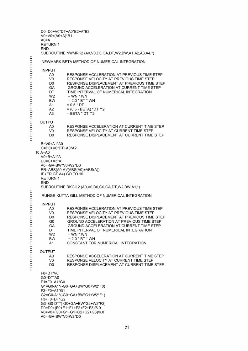
21

D0=D0+V0*DT+A0*B2+A*B3 V0=V0+(A0+A)*B1 A0=A RETURN 1 END SUBROUTINE NWMRK2 (A0,V0,D0,GA,DT,W2,BW,A1,A2,A3,A4,*) C C NEWMARK BETA METHOD OF NUMERICAL INTEGRATION C C INPPUT C A0 RESPONSE ACCLERATION AT PREVIOUS TIME STEP C V0 RESPONSE VELOCITY AT PREVIOUS TIME STEP C D0 RESPONSE DISPLACEMENT AT PREVIOUS TIME STEP C GA GROUND ACCELERATION AT CURRENT TIME STEP C DT TIME INTERVAL OF NUMERICAL INTEGRATION C W2 = WN * WN C BW = 2.0 * BT * WN C A1 = 0.5 * DT C A2 = (0.5 - BETA) *DT **2 C A3 = BETA * DT **2 C C OUTPUT C A0 RESPONSE ACCELERATION AT CURRENT TIME STEP C V0 RESPONSE VELOCITY AT CURRENT TIME STEP C D0 RESPONSE DISPLACEMENT AT CURRENT TIME STEP C B=V0+A1*A0 C=D0+V0*DT+A0*A2 10 A=A0 V0=B+A1*A D0=C+A3*A A0=-GA-BW*V0-W2*D0 ER=ABS(A0-A)/(ABS(A0)+ABS(A)) IF (ER.GT.A4) GO TO 10 RETURN 1 END SUBROUTINE RKGIL2 (A0,V0,D0,G0,GA,DT,W2,BW,A1,*) C C RUNGE-KUTTA-GILL METHOD OF NUMERICAL INTEGRATION C C INPPUT C A0 RESPONSE ACCLERATION AT PREVIOUS TIME STEP C V0 RESPONSE VELOCITY AT PREVIOUS TIME STEP C D0 RESPONSE DISPLACEMENT AT PREVIOUS TIME STEP C G0 GROUND ACCELERATION AT PREVIOUS TIME STEP C GA GROUND ACCELERATION AT CURRENT TIME STEP C DT TIME INTERVAL OF NUMERICAL INTEGRATION C W2 = WN * WN C BW = 2.0 * BT * WN C A1 CONSTANT FOR NUMERICAL INTEGRATION C C OUTPUT C A0 RESPONSE ACCELERATION AT CURRENT TIME STEP C V0 RESPONSE VELOCITY AT CURRENT TIME STEP C D0 RESPONSE DISPLACEMENT AT CURRENT TIME STEP C F0=DT*V0 G0=DT*A0 F1=F0+A1*G0 G1=G0-A1*(-G0+GA+BW*G0+W2*F0) F2=F0+A1*G1 G2=G0-A1*(-G0+GA+BW*G1+W2*F1) F3=F0+DT*G2 G3=G0-DT*(-G0+GA+BW*G2+W2*F2) D0=D0+(F0+F1+F1+F2+F2+F3)/6.0 V0=V0+(G0+G1+G1+G2+G2+G3)/6.0 A0=-GA-BW*V0-W2*D0

22

RETURN 1 END

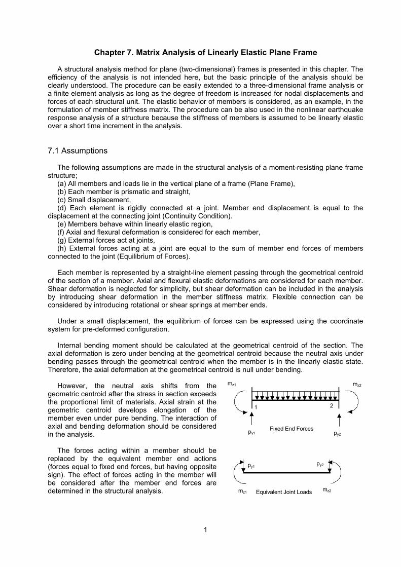
1

Chapter 7. Matrix Analysis of Linearly Elastic Plane Frame

A structural analysis method for plane (two-dimensional) frames is presented in this chapter. The efficiency of the analysis is not intended here, but the basic principle of the analysis should be clearly understood. The procedure can be easily extended to a three-dimensional frame analysis or a finite element analysis as long as the degree of freedom is increased for nodal displacements and forces of each structural unit. The elastic behavior of members is considered, as an example, in the formulation of member stiffness matrix. The procedure can be also used in the nonlinear earthquake response analysis of a structure because the stiffness of members is assumed to be linearly elastic over a short time increment in the analysis. 7.1 Assumptions

The following assumptions are made in the structural analysis of a moment-resisting plane frame structure;

(a) All members and loads lie in the vertical plane of a frame (Plane Frame), (b) Each member is prismatic and straight, (c) Small displacement, (d) Each element is rigidly connected at a joint. Member end displacement is equal to the

displacement at the connecting joint (Continuity Condition). (e) Members behave within linearly elastic region, (f) Axial and flexural deformation is considered for each member, (g) External forces act at joints, (h) External forces acting at a joint are equal to the sum of member end forces of members

connected to the joint (Equilibrium of Forces). Each member is represented by a straight-line element passing through the geometrical centroid

of the section of a member. Axial and flexural elastic deformations are considered for each member. Shear deformation is neglected for simplicity, but shear deformation can be included in the analysis by introducing shear deformation in the member stiffness matrix. Flexible connection can be considered by introducing rotational or shear springs at member ends.

Under a small displacement, the equilibrium of forces can be expressed using the coordinate

system for pre-deformed configuration. Internal bending moment should be calculated at the geometrical centroid of the section. The

axial deformation is zero under bending at the geometrical centroid because the neutral axis under bending passes through the geometrical centroid when the member is in the linearly elastic state. Therefore, the axial deformation at the geometrical centroid is null under bending.

However, the neutral axis shifts from the

geometric centroid after the stress in section exceeds the proportional limit of materials. Axial strain at the geometric centroid develops elongation of the member even under pure bending. The interaction of axial and bending deformation should be considered in the analysis.

The forces acting within a member should be

replaced by the equivalent member end actions (forces equal to fixed end forces, but having opposite sign). The effect of forces acting in the member will be considered after the member end forces are determined in the structural analysis.

2 1

mz1 mz2

py1 py2Fixed End Forces

mz2

py1 py2

mz1 Equivalent Joint Loads

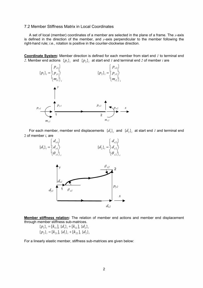
2

7.2 Member Stiffness Matrix in Local Coordinates

A set of local (member) coordinates of a member are selected in the plane of a frame. The x-axis is defined in the direction of the member, and y-axis perpendicular to the member following the right-hand rule; i.e., rotation is positive in the counter-clockwise direction. Coordinate System: Member direction is defined for each member from start end 1 to terminal end 2. Member end actions { }p i1 and { }p i2 at start end 1 and terminal end 2 of member i are

{ }pppm

i

x

y

z i

1

1

1

1

=

{ }pppm

i

x

y

z i

2

2

2

2

=

For each member, member end displacements { }d i1 and { }d i2 at start end 1 and terminal end

2 of member i, are

{ }dddi

x

y

z i

1

1

1

1

=

θ

{ }dddi

x

y

z i

2

2

2

2

=

θ

Member stiffness relation: The relation of member end actions and member end displacement through member stiffness sub-matrices.

{ } [ ] { } [ ] { }p k d k di i i i i1 11 1 12 2= + { } [ ] { } [ ] { }p k d k di i i i i2 21 1 22 2= +

For a linearly elastic member, stiffness sub-matrices are given below:

y

x px1 px2py1 py2

mz1 mz2

1 2

dy1

dx1

dx2

py2 θz1

θz2y

x

1

2

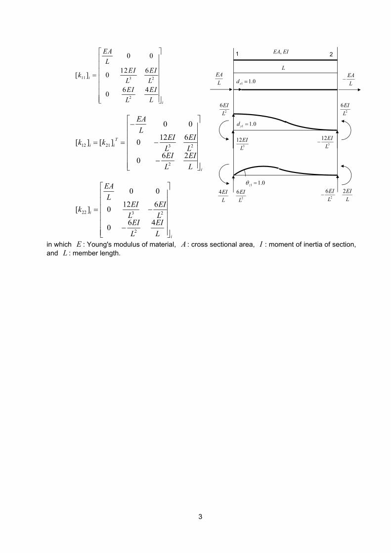
3

11 3 2

2

0 0

12 6[ ] 0

6 40

i

i

EAL

EI EIkL LEI EIL L

=

[ ] [ ]k k

EAL

EIL

EIL

EIL

EIL

i iT

i

12 21 3 2

2

0 0

0 12 6

0 6 2

= =

−

−

−

[ ]k

EAL

EIL

EIL

EIL

EIL

i

i

22 3 2

2

0 0

0 12 6

0 6 4

= −

−

in which E : Young's modulus of material, A : cross sectional area, I : moment of inertia of section, and L : member length.

1 1.0xd =EAL

EAL

−

1 1.0yd =

3

12EIL

3

12EIL

−

2

6EIL2

6EIL

1 1.0zθ =

1 2,EA EI

L

2

6EIL 2

6EIL

−4EIL

2EIL

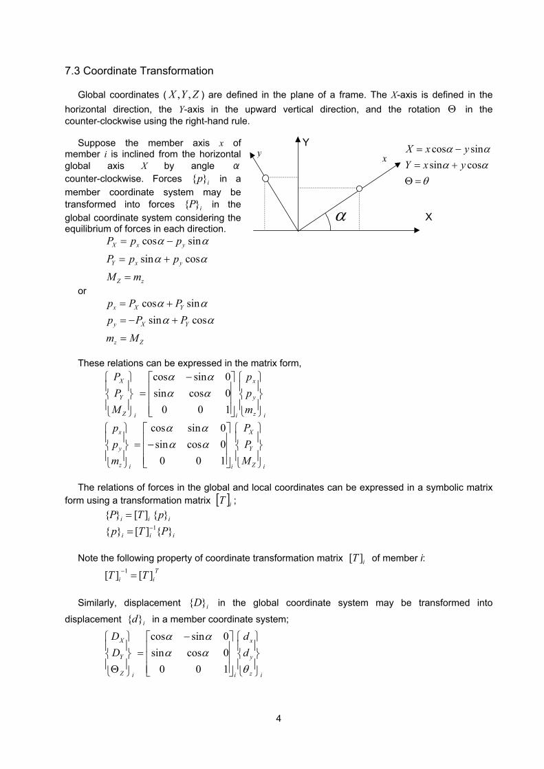
4

7.3 Coordinate Transformation

Global coordinates ( , ,X Y Z ) are defined in the plane of a frame. The X-axis is defined in the horizontal direction, the Y-axis in the upward vertical direction, and the rotation Θ in the counter-clockwise using the right-hand rule.

Suppose the member axis x of member i is inclined from the horizontal global axis X by angle α counter-clockwise. Forces { }p i in a member coordinate system may be transformed into forces { }P i in the global coordinate system considering the equilibrium of forces in each direction.

cos sinsin cos

X x y

Y x y

Z z

P p p

P p p

M m

α α

α α

= −

= +

=

or cos sin

sin cosx X Y

y X Y

z Z

p P Pp P Pm M

α αα α

= += − +

=

These relations can be expressed in the matrix form,

iz

y

x

iiZ

Y

X

mpp

MPP

−=

1000cossin0sincos

αααα

cos sin 0sin cos 00 0 1

x X

y Y

z Zi i i

p Pp Pm M

α αα α

= −

The relations of forces in the global and local coordinates can be expressed in a symbolic matrix

form using a transformation matrix [ ]iT ; { } [ ] { }P T pi i i=

iii PTp }{][}{ 1−=

Note the following property of coordinate transformation matrix [ ]T i of member i: 1[ ] [ ] T

i iT T− = Similarly, displacement iD}{ in the global coordinate system may be transformed into

displacement id}{ in a member coordinate system;

iz

y

x

iiZ

Y

X

dd

DD

−=

Θ θαααα

1000cossin0sincos

X

Yx y

α

θαααα

=Θ+=−=

cossinsincos

yxYyxX

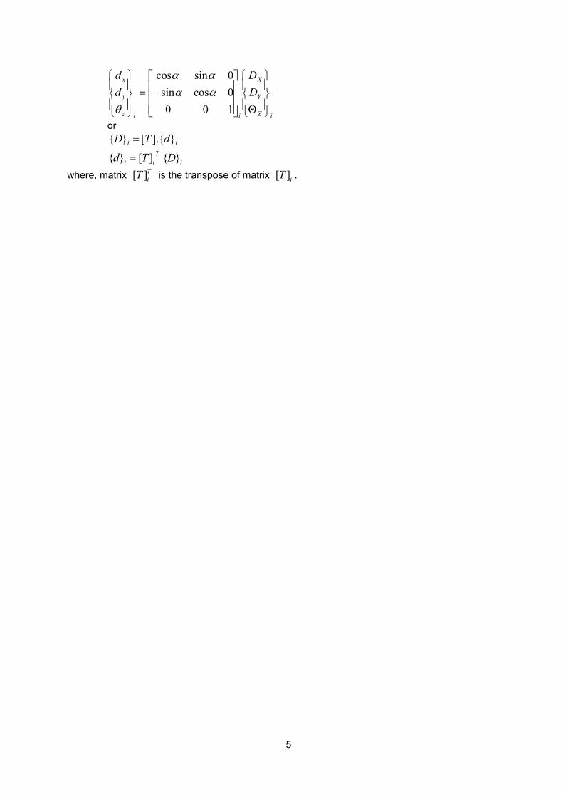
5

iZ

Y

X

iiz

y

x

DD

dd

Θ

−=

1000cossin0sincos

αααα

θ

or iii dTD }{][}{ =

{ } [ ] { }d T Di iT

i=

where, matrix [ ]TiT is the transpose of matrix [ ]iT .

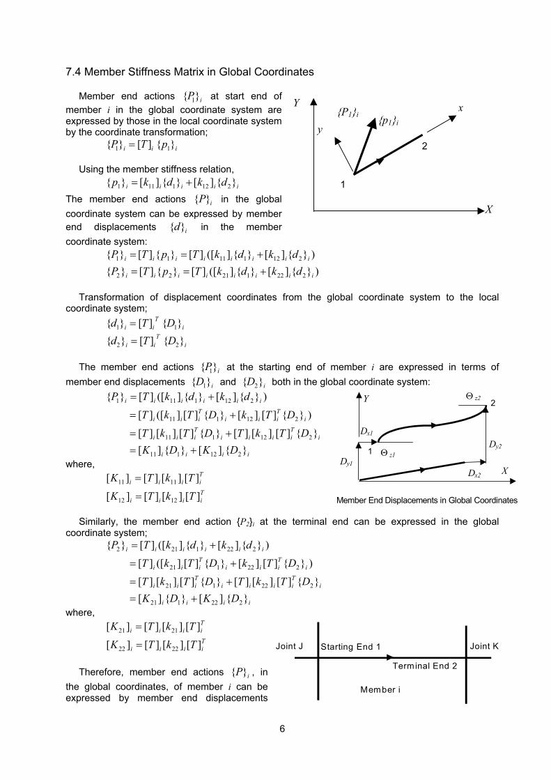
6

7.4 Member Stiffness Matrix in Global Coordinates

Member end actions { }P i1 at start end of member i in the global coordinate system are expressed by those in the local coordinate system by the coordinate transformation;

{ } [ ] { }P T pi i i1 1=

Using the member stiffness relation, iiiii dkdkp }{][}{][}{ 2121111 +=

The member end actions { }iP in the global coordinate system can be expressed by member end displacements { }id in the member coordinate system:

)}{][}{]([][}{][}{)}{][}{]([][}{][}{

22212122

21211111

iiiiiiii

iiiiiiii

dkdkTpTPdkdkTpTP

+==+==

Transformation of displacement coordinates from the global coordinate system to the local

coordinate system; { } [ ] { }d T Di i

Ti1 1=

{ } [ ] { }d T Di iT

i2 2=

The member end actions { }P i1 at the starting end of member i are expressed in terms of member end displacements { }D i1 and { }D i2 both in the global coordinate system:

iiii

iTiiii

Tiii

iTiii

Tiii

iiiiii

DKDKDTkTDTkT

DTkDTkT

dkdkTP

}{][}{][}{][][][}{][][][

)}{][][}{][]([][

)}{][}{]([][}{

212111

212111

212111

2121111

+=+=

+=

+=

where,

Tiiii

Tiiii

TkTK

TkTK

][][][][

][][][][

1212

1111

=

=

Similarly, the member end action {P2}i at the terminal end can be expressed in the global

coordinate system;

iiii

iTiiii

Tiii

iTiii

Tiii

iiiiii

DKDKDTkTDTkT

DTkDTkT

dkdkTP

}{][}{][}{][][][}{][][][

)}{][][}{][]([][

)}{][}{]([][}{

222121

222121

222121

2221212

+=+=

+=

+=

where,

Tiiii

Tiiii

TkTK

TkTK

][][][][

][][][][

2222

2121

=

=

Therefore, member end actions iP}{ , in

the global coordinates, of member i can be expressed by member end displacements

X

Y x

y {p1}i

{P1}i

1

2

Dy1

Dx1

Dx2

Dy2Θ z1

Θ z2Y

X

1

2

Member End Displacements in Global Coordinates

Joint J Joint KStarting End 1

Terminal End 2

Member i

7

iD}{ using member stiffness matrix iK ][ in the global coordinates;

iii

iii

DD

KKKK

PP

DKP

=

=

2

1

2221

1211

2

1

}{][}{

where, 2,1,]][[][][ == kjforTkTK T

ijkijk

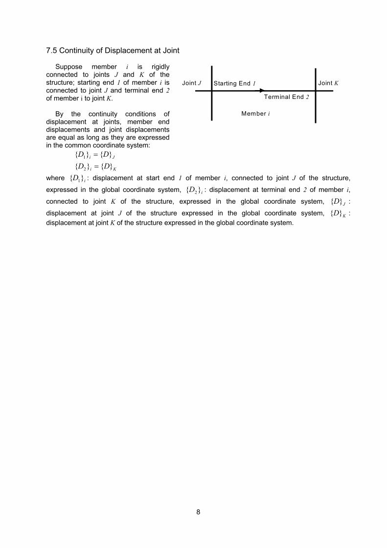
8

7.5 Continuity of Displacement at Joint

Suppose member i is rigidly connected to joints J and K of the structure; starting end 1 of member i is connected to joint J and terminal end 2 of member i to joint K.

By the continuity conditions of displacement at joints, member end displacements and joint displacements are equal as long as they are expressed in the common coordinate system:

Ki

Ji

DDDD

}{}{}{}{

2

1

==

where iD }{ 1 : displacement at start end 1 of member i, connected to joint J of the structure,

expressed in the global coordinate system, iD }{ 2 : displacement at terminal end 2 of member i,

connected to joint K of the structure, expressed in the global coordinate system, JD}{ :

displacement at joint J of the structure expressed in the global coordinate system, KD}{ : displacement at joint K of the structure expressed in the global coordinate system.

Joint J Joint K Starting End 1

Terminal End 2

Member i

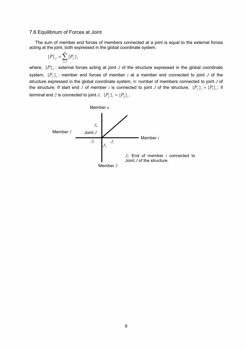
9

7.6 Equilibrium of Forces at Joint

The sum of member end forces of members connected at a joint is equal to the external forces acting at the joint, both expressed in the global coordinate system.

∑=

=n

iiJJ PP

1

}{}{

where, JP}{ : external forces acting at joint J of the structure expressed in the global coordinate

system, iJP }{ : member end forces of member i at a member end connected to joint J of the structure expressed in the global coordinate system, n: number of members connected to joint J of the structure. If start end 1 of member i is connected to joint J of the structure, iiJ PP }{}{ 1= ; if

terminal end 2 is connected to joint J, iiJ PP }{}{ 2= .

Member 1

Member 2

Member i

Member n

Joint J

J1 J2

Ji

Jn

Ji: End of member i connected to Joint J of the structure.

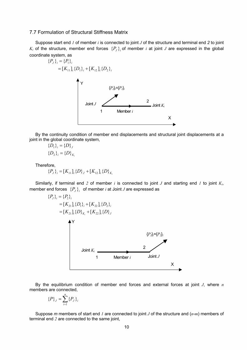
10

7.7 Formulation of Structural Stiffness Matrix

Suppose start end 1 of member i is connected to joint J of the structure and terminal end 2 to joint Ki of the structure, member end forces iJP }{ of member i at joint J are expressed in the global coordinate system, as

iiii

iiJ

DKDKPP

}{][}{][}{}{

212111

1

+==

By the continuity condition of member end displacements and structural joint displacements at a

joint in the global coordinate system,

iKi

Ji

DDDD

}{}{}{}{

2

1

==

Therefore,

iKiJiiJ DKDKP }{][}{][}{ 1211 +=

Similarly, if terminal end 2 of member i is connected to joint J and starting end 1 to joint Ki, member end forces iJP }{ of member i at Joint J are expressed as

2

21 1 22 2

21 22

{ } { }[ ] { } [ ] { }[ ] { } [ ] { }

i

J i i

i i i i

i K i J

P PK D K DK D K D

== += +

By the equilibrium condition of member end forces and external forces at joint J, where n

members are connected,

∑=

=n

iiJJ PP

1

}{}{

Suppose m members of start end 1 are connected to joint J of the structure and (n-m) members of

terminal end 2 are connected to the same joint,

Member i 1

2 Joint J Joint Ki

{PJ}i={P1}i

X

Y

Member i 1

2

Joint J Joint Ki

{PJ}i={P2}i

X

Y

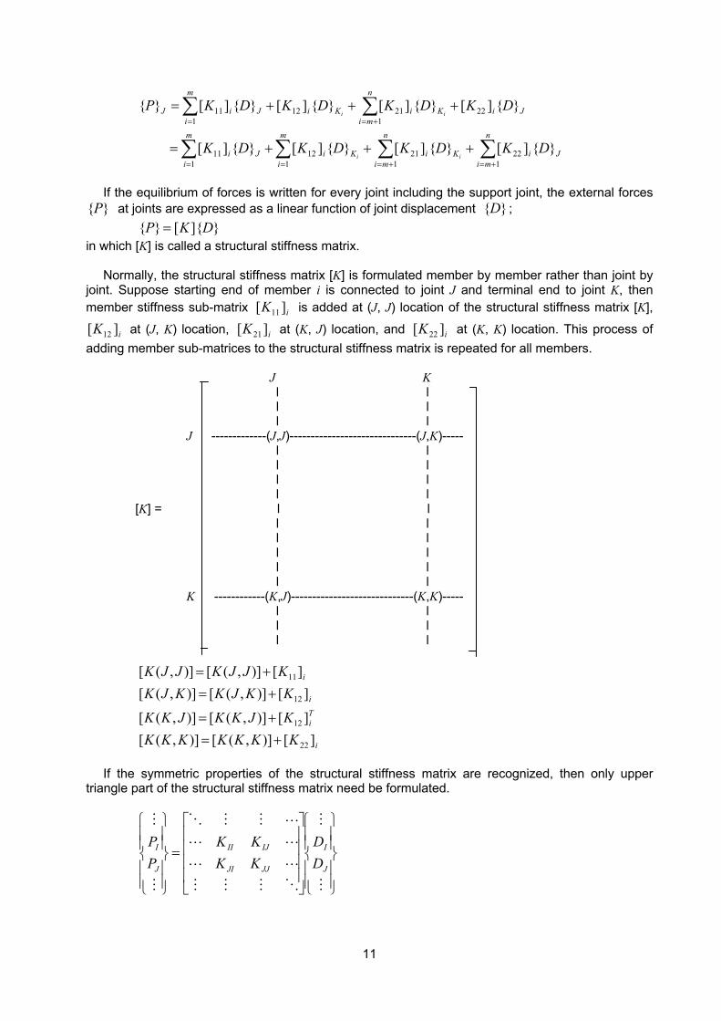
11

∑∑∑ ∑

∑∑

+=+== =

+==

+++=

+++=

n

miJiK

n

mii

m

i

m

iKiJi

JiK

n

mii

m

iKiJiJ

DKDKDKDK

DKDKDKDKP

ii

ii

122

121

1 11211

221

211

1211

}{][}{][}{][}{][

}{][}{][}{][}{][}{

If the equilibrium of forces is written for every joint including the support joint, the external forces }{P at joints are expressed as a linear function of joint displacement }{D ;

}]{[}{ DKP = in which [K] is called a structural stiffness matrix.

Normally, the structural stiffness matrix [K] is formulated member by member rather than joint by joint. Suppose starting end of member i is connected to joint J and terminal end to joint K, then member stiffness sub-matrix iK ][ 11 is added at (J, J) location of the structural stiffness matrix [K],

iK ][ 12 at (J, K) location, iK ][ 21 at (K, J) location, and iK ][ 22 at (K, K) location. This process of adding member sub-matrices to the structural stiffness matrix is repeated for all members.

J K l l l l l l J -------------(J,J)------------------------------(J,K)----- l l l l l l l l [K] = l l l l l l l l l l l l K ------------(K,J)-----------------------------(K,K)----- l l l l l l

i

Ti

i

i

KKKKKKKKJKKJKK

KKJKKJKKJJKJJK

][)],([)],([][)],([)],([

][)],([)],([][)],([)],([

22

12

12

11

+=+=

+=+=

If the symmetric properties of the structural stiffness matrix are recognized, then only upper

triangle part of the structural stiffness matrix need be formulated.

=

M

M

OMMM

LL

LL

LMMO

M

M

J

I

JJJI

IJII

J

I

DD

KKKK

PP

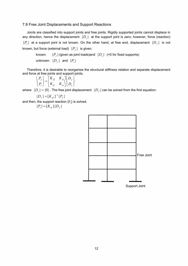
12

7.8 Free Joint Displacements and Support Reactions

Joints are classified into support joints and free joints. Rigidly supported joints cannot displace in any direction, hence the displacement }{ sD at the support joint is zero; however, force (reaction)

}{ sP at a support joint is not known. On the other hand, at free end, displacement }{ fD is not

known, but force (external load) }{ fP is given.

known: }{ fP (given as joint loads)and }{ sD (=0 for fixed supports)

unknown: }{ fD and }{ sP

Therefore, it is desirable to reorganize the structural stiffness relation and separate displacement and force at free joints and support joints;

=

s

f

sssf

fsff

s

f

DD

KKKK

PP

where }0{}{ =sD . The free joint displacement }{ fD can be solved from the first equation:

}{][}{ 1ffff PKD −=

and then, the support reaction {Ps} is solved. }]{[}{ fsfs DKP =

Support Joint

Free Joint

13

7.9 Member End Actions

Once joint displacements are all calculated, then member end actions in the local coordinate system can be calculated using joint displacements and member stiffness matrix.

The member end actions and displacements relation for member i is

iiiii

iiiii

dkdkpdkdkp

}{][}{][}{}{][}{][}{

2221212

2121111

+=+=

If starting end 1 of the member is connected

to joint J and terminal end 2 to joint K, using the continuity condition of displacement at joint an transformation of coordinates, joint end displacements in local coordinates are expressed

K

Tii

JTii

DTd

DTd

}{][}{

}{][}{

2

1

=

=

Combining the above two relations;

K

TiiJ

Tiii

KTiiJ

Tiii

DTkDTkp

DTkDTkp

}{][][}{][][}{

}{][][}{][][}{

22212

12111

+=

+=

The bending moment distributes linearly along the member because no intermediate loads act in

the member.

If intermediate loads act in the member, the above member end actions should be added to the member actions of fixed-fixed member under the given intermediate loads.

Joint J Joint K Starting End 1

Terminal End 2

Member i

py2

px2

mz2

py1

px1 Member i

Structural Analysis

FEM1 FEM2

Stress due to member loading

mz1

Final Member Stresses

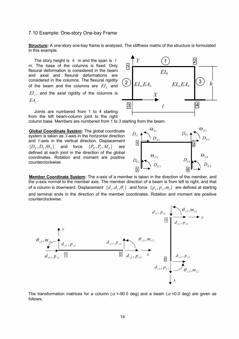
14

7.10 Example: One-story One-bay Frame

Structure: A one-story one-bay frame is analyzed. The stiffness matrix of the structure is formulated in this example.

The story height is h m and the span is l

m. The base of the columns is fixed. Only flexural deformation is considered in the beam and axial and flexural deformations are considered in the columns. The flexural rigidity of the beam and the columns are bEI and

cEI , and the axial rigidity of the columns is

cEA . Joints are numbered from 1 to 4 starting

from the left beam-column joint to the right column base. Members are numbered from 1 to 3 starting from the beam.

Global Coordinate System: The global coordinate system is taken as X-axis in the horizontal direction and Y-axis in the vertical direction. Displacement { , , }X Y ZD D Θ and force { , , }X Y ZP P M are defined at each joint in the direction of the global coordinates. Rotation and moment are positive counterclockwise.

Member Coordinate System: The x-axis of a member is taken in the direction of the member, and the y-axis normal to the member axis. The member direction of a beam is from left to right, and that of a column is downward. Displacement { , , }x y zd d θ and force { , , }x y zp p m are defined at starting and terminal ends in the direction of the member coordinates. Rotation and moment are positive counterclockwise.

The transformation matrices for a column (α =-90.0 deg) and a beam (α =0.0 deg) are given as follows;

EIb

EIc,EAc EIc,EAc h

l

12

3 4

X

Y 1

2 3

1 2

3 4

1XD1YD

1ZΘ

2XD2YD

2ZΘ

3XD3YD

3ZΘ

4XD4YD

4ZΘ

1 1,x xd p

1 1,y yd p1 1,z zmθ

2 2,x xd p

2 2,y yd p 2 2,z zmθ

1 2 x

y 1 1,y yd p

1 1,x xd p 1 1,z zmθ

2 2,y yd p

2 2,x xd p 2 2,z zmθ

1

2

y

x

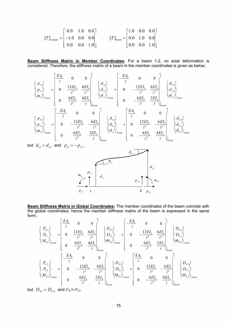
15

0.0 1.0 0.0 1.0 0.0 0.0[ ] 1.0 0.0 0.0 [ ] 0.0 1.0 0.0

0.0 0.0 1.0 0.0 0.0 1.0column beamT T

= − =

Beam Stiffness Matrix in Member Coordinates: For a beam 1-2, no axial deformation is considered. Therefore, the stiffness matrix of a beam in the member coordinates is given as below;

1 1 2

1 1 23 2 3 2

1 1 2

2 2

2

2

2

0 0 0 0

12 6 12 60 0

6 4 6 20 0

b b

x x xb b b b

y y y

z z zbeam beam beamb b b b

beam beam

x

y

z

EA EA

p d dEI EI EI EIp d d

m EI EI EI EI

ppm

θ θ

− = + −

−

l l

l l l l

l l l l

1 2

1 23 2 3 2

1 2

2 2

0 0 0 0

12 6 12 60 0

6 2 6 40 0

b b

x xb b b b

y y

z zbeam beam beamb b b b

beam beam

EA EA

d dEI EI EI EId d

EI EI EI EIθ θ

− = − − + −

−

l l

l l l l

l l l l

but 1 2x xd d= and 1 2x xp p= − .

1 21xp

1yp 1zm

2zθ

1zθ

2xp

2zm2yp1yd

2yd

Beam Stiffness Matrix in Global Coordinates: The member coordinates of the beam coincide with the global coordinates; hence the member stiffness matrix of the beam is expressed in the same form;

1 1 2

1 1 23 2 3 2

1 1 2

2 2

2

2

2

0 0 0 0

12 6 12 60 0

6 4 6 20 0

b b

X X Xb b b b

Y Y Y

Z Z Zbeam beam beamb b b b

beam beam

X

Y

Z

EA EA

P D DEI EI EI EIP D D

M EI EI EI EI

PP

M

− = + − Θ Θ

−

l l

l l l l

l l l l

1 2

1 23 2 3 2

1 2

2 2

0 0 0 0

12 6 12 60 0

6 2 6 40 0

b b

X Xb b b b

Y Y

Z Zbeam beam beamb b b b

beam beam

EA EA

D DEI EI EI EID D

EI EI EI EI

− = − − + − Θ Θ

−

l l

l l l l

l l l l

but 1 2X XD D= and PX1=-PX2.

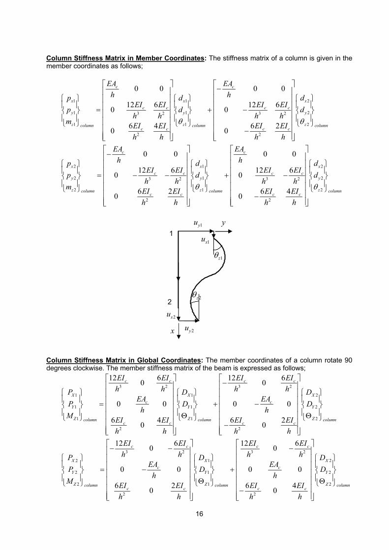
16

Column Stiffness Matrix in Member Coordinates: The stiffness matrix of a column is given in the member coordinates as follows;

1 1 2

1 1 23 2 3 2

1 1 2

2 2

2

2

2

0 0 0 0

12 6 12 60 0

6 4 6 20 0

c c

x x xc c c c

y y y

z z zcolumn column columnc c c c

x

y

z c

EA EAh hp d d

EI EI EI EIp d dh h h h

m EI EI EI EIh h h h

ppm

θ θ

− = + −

−

1 2

1 23 2 3 2

1 2

2 2

0 0 0 0

12 6 12 60 0

6 2 6 40 0

c c

x xc c c c

y y

z zolumn column columnc c c c

EA EAh hd d

EI EI EI EId dh h h h

EI EI EI EIh h h h

θ θ

− = − − + −

−

1zθ

2zθ

1yu

2yu

1A

2

x

y

1xu

2xu

Column Stiffness Matrix in Global Coordinates: The member coordinates of a column rotate 90 degrees clockwise. The member stiffness matrix of the beam is expressed as follows;

3 2 3 2

1 1 2

1 1 2

1 1 2

2 2

2

2

2

12 6 12 60 0

0 0 0 0

6 4 6 20 0

c c c c

X X Xc c

Y Y Y

Z Z Zcolumn column columnc c c c

X

Y

Z c

EI EI EI EIh h h hP D D

EA EAP D Dh h

M EI EI EI EIh h h h

PP

M

− = + − Θ Θ

−

3 2 3 2

1 2

1 2

1 2

2 2

12 6 12 60 0

0 0 0 0

6 2 6 40 0

c c c c

X Xc c

Y Y

Z Zolumn column columnc c c c

EI EI EI EIh h h hD D

EA EAD Dh h

EI EI EI EIh h h h

− − − = − + Θ Θ

−

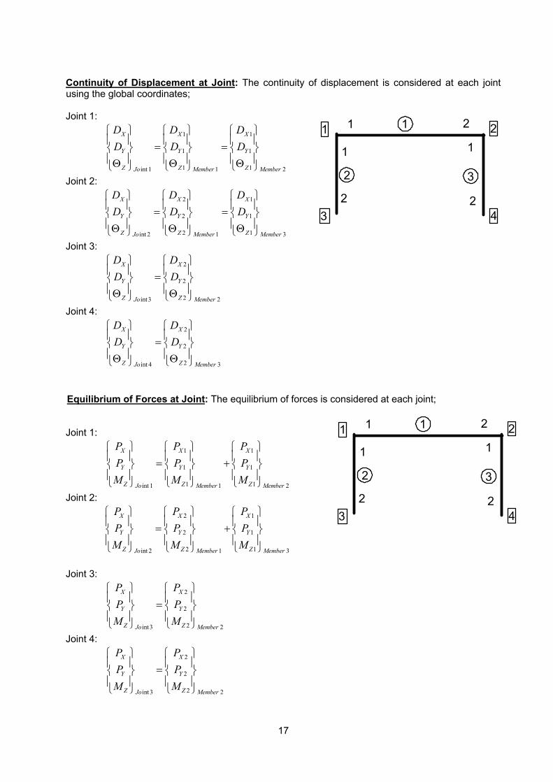
17

Continuity of Displacement at Joint: The continuity of displacement is considered at each joint using the global coordinates; Joint 1:

1 1

1 1

1 1int 1 1 2

X X X

Y Y Y

Z Z ZJo Member Member

D D DD D D

= = Θ Θ Θ

Joint 2:

2 1

2 1

2 1int 2 1 3

X X X

Y Y Y

Z Z ZJo Member Member

D D DD D D

= = Θ Θ Θ

Joint 3:

2

2

2int3 2

X X

Y Y

Z ZJo Member

D DD D

= Θ Θ

Joint 4:

2

2

2int 4 3

X X

Y Y

Z ZJo Member

D DD D

= Θ Θ

Equilibrium of Forces at Joint: The equilibrium of forces is considered at each joint; Joint 1:

1 1

1 1

1 1int 1 1 2

X X X

Y Y Y

Z Z ZJo Member Member

P P PP P P

M M M

= +

Joint 2:

2 1

2 1

2 1int 2 1 3

X X X

Y Y Y

Z Z ZJo Member Member

P P PP P P

M M M

= +

Joint 3:

2

2

2int3 2

X X

Y Y

Z ZJo Member

P PP P

M M

=

Joint 4:

2

2

2int3 2

X X

Y Y

Z ZJo Member

P PP P

M M

=

1 2

3 4

1 2

1

2

1

2

1

2 3

1 2

3 4

1 2

1

2

1

2

1

2 3

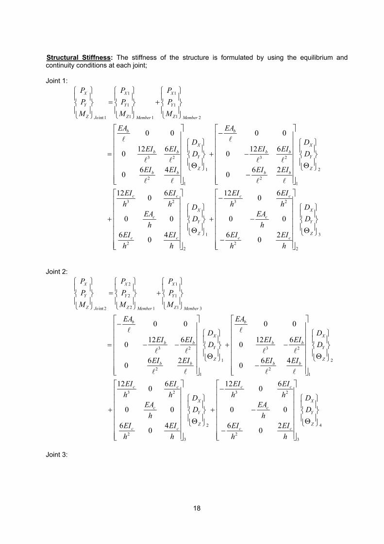
18

Structural Stiffness: The stiffness of the structure is formulated by using the equilibrium and continuity conditions at each joint; Joint 1:

1 1

1 1

1 1int 1 1 2

3 2 3 2

1

2 21 1

0 0 0 0

12 6 12 60 0

6 4 6 20 0

X X X

Y Y Y

Z Z ZJo Member Member

b b

Xb b b b

Y

Zb b b b

P P PP P P

M M M

EA EA

DEI EI EI EID

EI EI EI EI

= +

− = + − Θ

−

l l

l l l l

l l l l

2

3 2 3 2

1 3

2 22 2

12 6 12 60 0

0 0 0 0

6 4 6 20 0

X

Y

Z

c c c c

X Xc c

Y Y

Z Zc c c c

DD

EI EI EI EIh h h hD D

EA EAD Dh h

EI EI EI EIh h h h

Θ

− + + − Θ Θ

−

Joint 2:

2 1

2 1

2 1int 2 1 3

3 2 3 2

1

2 21

0 0 0 0

12 6 12 60 0

6 2 6 40 0

X X X

Y Y Y

Z Z ZJo Member Member

b b

Xb b b b

Y

Zb b b b

P P PP P P

M M M

EA EA

DEI EI EI EID

EI EI EI EI

= +

− = − − + − Θ

−

l l

l l l l

l l l l

2

1

3 2 3 2

2 4

2 23 3

12 6 12 60 0

0 0 0 0

6 4 6 20 0

X

Y

Z

c c c c

X Xc c

Y Y

Z Zc c c c

DD

EI EI EI EIh h h hD D

EA EAD Dh h

EI EI EI EIh h h h

Θ

− + + − Θ Θ

−

Joint 3:

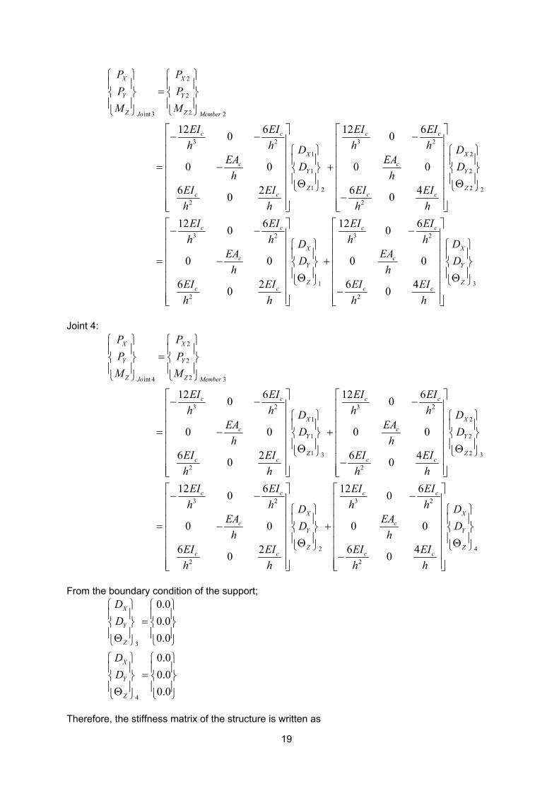
19

2

2

2int3 2

3 2 3 2

1 2

1 2

1 22 2

2 2

12 6 12 60 0

0 0 0 0

6 2 6 40 0

12

X X

Y Y

Z ZJo Member

c c c c

X Xc c

Y Y

Z Zc c c c

P PP P

M M

EI EI EI EIh h h hD D

EA EAD Dh h

EI EI EI EIh h h h

=

− − − = − + Θ Θ

−

−

=

3 2 3 2

1 3

2 2

6 12 60 0

0 0 0 0

6 2 6 40 0

c c c c

X Xc c

Y Y

Z Zc c c c

EI EI EI EIh h h hD D

EA EAD Dh h

EI EI EI EIh h h h

− − − + Θ Θ

−

Joint 4:

2

2

2int 4 3

3 2 3 2

1 2

1 2

1 23 3

2 2

12 6 12 60 0

0 0 0 0

6 2 6 40 0

12

X X

Y Y

Z ZJo Member

c c c c

X Xc c

Y Y

Z Zc c c c

P PP P

M M

EI EI EI EIh h h hD D

EA EAD Dh h

EI EI EI EIh h h h

=

− − − = − + Θ Θ

−

−

=

3 2 3 2

2 4

2 2

6 12 60 0

0 0 0 0

6 2 6 40 0

c c c c

X Xc c

Y Y

Z Zc c c c

EI EI EI EIh h h hD D

EA EAD Dh h

EI EI EI EIh h h h

− − − + Θ Θ

−

From the boundary condition of the support;

3

4

0.00.00.0

0.00.00.0

X

Y

Z

X

Y

Z

DD

DD

= Θ

= Θ

Therefore, the stiffness matrix of the structure is written as

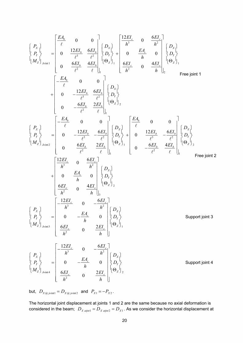
20

3 2

3 2

int 1 1 1

2 21 2

3 2

2

12 600 0

12 60 0 0

6 4 6 40 0

0 0

12 60

6 20

c cb

X X Xb b c

Y Y Y

Z Z ZJob b c c

b

b b

b b

EI EIEAh hP D D

EI EI EAP D Dh

M EI EI EI EIh h

EA

EI EI

EI EI

= + Θ Θ

−

+ −

−

l

l l

l l

l

l l

l l

2

1

X

Y

Z

DD

Θ

Free joint 1

3 2 3 2

int 2 1 2

2 21 1

3 2

2

0 0 0 0

12 6 12 60 0

6 2 6 40 0

12 60

0 0

6 40

b b

X X Xb b b b

Y Y Y

Z Z ZJob b b b

c c

c

c c

EA EA

P D DEI EI EI EIP D D

M EI EI EI EI

EI EIh h

EAh

EI EIh h

− = − − + − Θ Θ

−

+

l l

l l l l

l l l l

2

3

X

Y

Z

DD

Θ

Free joint 2

3 2

int3 1

2

12 60

0 0

6 20

c c

X Xc

Y Y

Z ZJoc c

EI EIh hP D

EAP Dh

M EI EIh h

− − = − Θ

Support joint 3

3 2

int 4 2

2

12 60

0 0

6 20

c c

X Xc

Y Y

Z ZJoc c

EI EIh hP D

EAP Dh

M EI EIh h

− − = − Θ

Support joint 4

but, @ int1 @ int 2X jo X joD D= and 21 XX PP −= . The horizontal joint displacement at joints 1 and 2 are the same because no axial deformation is considered in the beam; 121 XatjntXatjntX DDD == . As we consider the horizontal displacement at

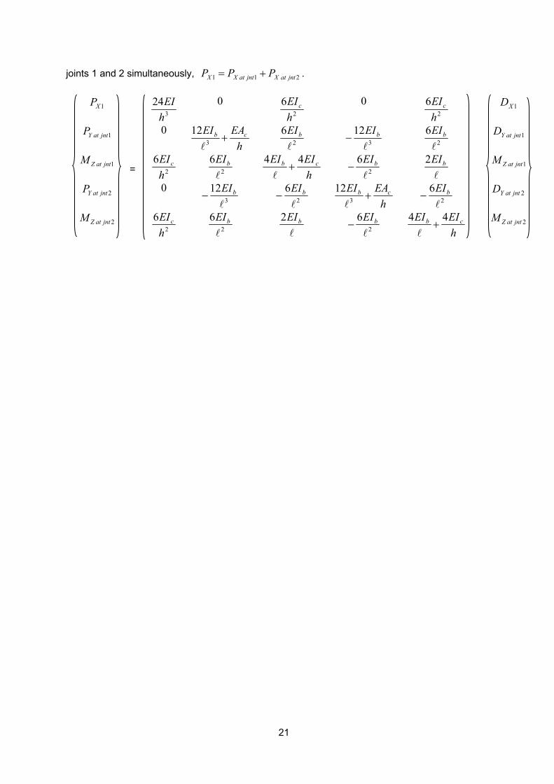
21

joints 1 and 2 simultaneously, 211 jntatXjntatXX PPP += .

1XP 3

24hEI

0

2

6hEIc

0 2

6hEIc 1XD

1jntatYP 0 h

EAEI cb +3

12l 2

6l

bEI 3

12l

bEI− 2

6l

bEI 1jntatYD

1jntatZM = 2

6hEIc 2

6l

bEI

hEIEI cb 44

+l 2

6l

bEI−

lbEI2

1jntatZM

2jntatYP 0 3

12l

bEI− 2

6l

bEI−

hEAEI cb +3

12l

2

6l

bEI− 2jntatYD

2jntatZM 2

6hEIc 2

6l

bEI

lbEI2

2

6l

bEI−

hEIEI cb 44

+l

2jntatZM

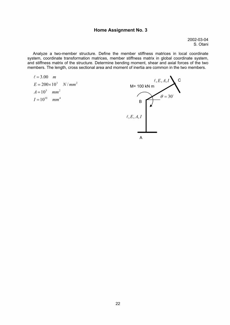
22

Home Assignment No. 3

2002-03-04 S. Otani

Analyze a two-member structure. Define the member stiffness matrices in local coordinate

system, coordinate transformation matrices, member stiffness matrix in global coordinate system, and stiffness matrix of the structure. Determine bending moment, shear and axial forces of the two members. The length, cross sectional area and moment of inertia are common in the two members.

410

25

23

1010

/1020000.3

mmImmA

mmNEm

=

=

×=

=l

A

B

C M= 100 kN m

IAE ,,,l

IAE ,,,l

30θ = o

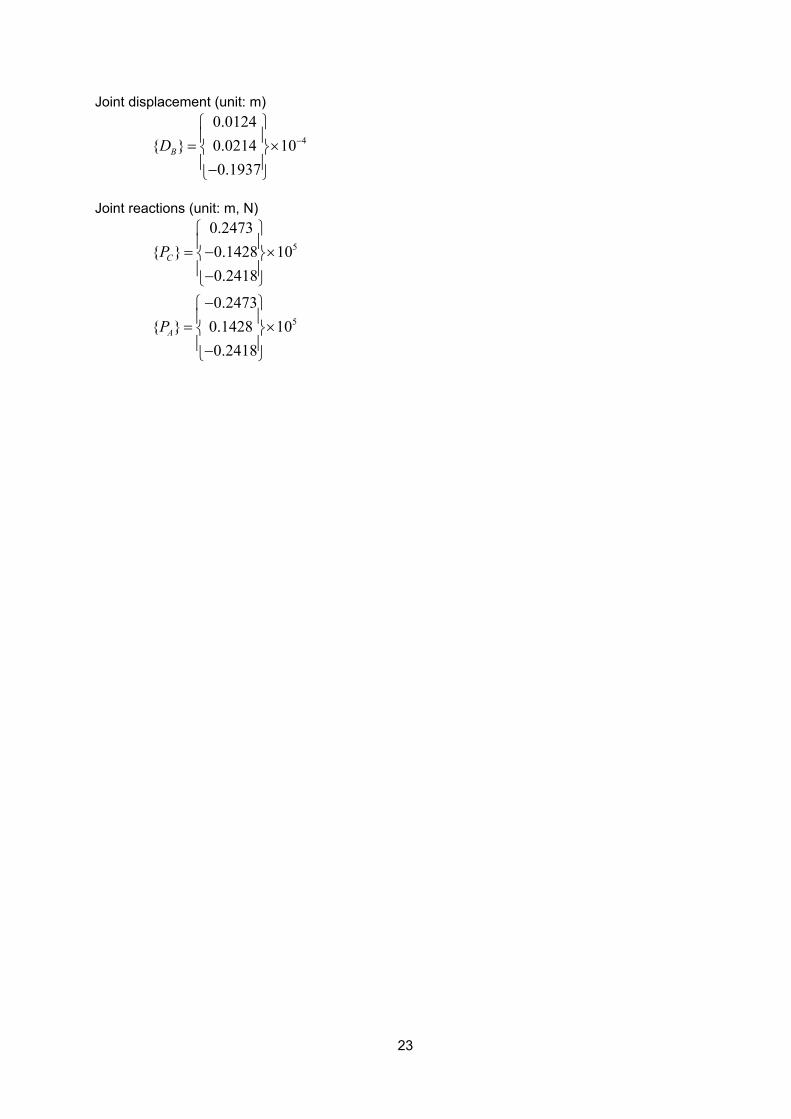
23

Joint displacement (unit: m)

4

0.0124{ } 0.0214 10

0.1937BD −

= × −

Joint reactions (unit: m, N)

5

5

0.2473{ } 0.1428 10

0.2418

0.2473{ } 0.1428 10

0.2418

C

A

P

P

= − × − − = × −

1

Chapter 8. Numerical Solution of Linear Equations

The equilibrium of a structure at time t is expressed as the equilibrium of internal force (structural resistance) { ( )}R t and external force { ( )}F t at structural nodes;

{ ( )} { ( )}F t R t= In a dynamic problem, the external force may be the sum of externally applied dynamic forces, and negative values of inertia and damping forces. The internal force is the restoring force of the structure. { ( )} { ( )} [ ]{ ( )} { ( )}F t P t M z t D t= − −&& where { ( )}P t : external force at time t, [ ]M : mass matrix, normally defined as lumped mass at each floor corresponding to the horizontal degree of freedom, { ( )}z t&& : absolute acceleration at mass point, { ( )}D t : damping resistance, normally defined at each floor for the horizontal degree of freedom. Damping force may be assumed to be proportional to velocity { ( )}x t& relative to the base of the structure, but the damping matrix may be made proportional to instantaneous stiffness in the horizontal degree of freedom. 8.1 Incremental Formulation

A nonlinear problem is normally solved by reducing the problem into a linear problem over a short time increment in an incremental approach.

For example, the equilibrium of dynamic forces at time 1it + can be written as

[ ]{ } { } { } { }0)()()( 111 =++ +++ iii tRtDtzM && The structural resistance and damping resistance may be written in incremental form; [ ] { } { } { } { } { } { } { }0)()()()())()(( 1111 =∆++∆+++ ++++ iiiiii tRtRtDtDetytxM &&&&

where 1( )iy t +&& : ground acceleration (given value as an input earthquake motion) at 1it + , and { }e : vector having unit value for all elements.

Separating the known quantities and unknown quantities, the equilibrium of dynamic forces at time 1+it can be written as

[ ]{ } { } { } [ ] { } { } { })()()()()()()( 11111 iiiiiii tRtDetyMtytRtDtxM −−−=∆+∆+ +++++ &&&&&&

The increment of internal force 1{ ( )}iR t +∆ may be approximated by product of tangent stiffness

[ ]it

K and incremental displacement { ( )}x t∆ relative to the base of the structure, and the

increment of damping force 1{ ( )}iD t +∆ by the product of tangent damping matrix [ ]it

C and

incremental velocity { ( )}x t∆& . [ ]{ } [ ] { } [ ] { } [ ] { } { } { })()()()()()()( 11111 iiiiititi tRtDetyMtytxKtxCtxM

ii−−−=∆+∆+ +++++ &&&&&&&

The incremental acceleration, velocity and displacement are related through a numerical

integration method assumed in the analysis. For example, using the Newmark β method scheme,

2 21 1

1 1

1{ ( )} { ( )} ( ) { ( )} { ( )}2

1 1{ ( )} { ( )} { ( )}2 2

i i i i

i i i

x t t x t t x t t x t

x t t x t t x t

β β+ +

+ +

∆ = ∆ + − ∆ + ∆

∆ = ∆ + ∆

& && &&

& && &&

where β is a constant of the Newmark Beta method, { ( )}ix t& and { ( )}ix t&& are known velocity and acceleration vectors at previous time step ti.

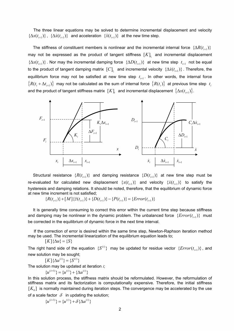
2

The three linear equations may be solved to determine incremental displacement and velocity 1{ ( )}ix t +∆ , 1{ ( )}ix t +∆& and acceleration 1{ ( )}ix t +&& at the new time step.

The stiffness of constituent members is nonlinear and the incremental internal force 1{ ( )}iR t +∆

may not be expressed as the product of tangent stiffness [ ]it

K and incremental displacement

1{ ( )}ix t +∆ . Nor may the incremental damping force 1{ ( )}iD t +∆ at new time step 1it + not be equal

to the product of tangent damping matrix [ ]it

C and incremental velocity 1{ ( )}ix t +∆& . Therefore, the

equilibrium force may not be satisfied at new time step 1it + . In other words, the internal force

{ })( 1+∆+ ii ttR may not be calculated as the sum of internal force { })( itR at previous time step it

and the product of tangent stiffness matrix [ ]tK and incremental displacement { })( 1+∆ itx .

ix 1ix +

iF

1iF +

1iF +∆

1i iK x +∆

1ix +∆ ix& 1ix +&

iD

1iD +

1iD +∆

1i iC x +∆&

1ix +∆&

x x&

iK iC

Structural resistance 1{ ( )}iR t + and damping resistance 1{ ( )}iD t + at new time step must be

re-evaluated for calculated new displacement 1{ ( )}ix t + and velocity 1{ ( )}ix t +& to satisfy the hysteresis and damping relations. It should be noted, therefore, that the equilibrium of dynamic force at new time increment is not satisfied;

1 1 1 1 1{ ( )} [ ]{ ( )} { ( )} { ( )} { ( )}i i i i iR t M z t D t P t Error t+ + + + ++ + − =&&

It is generally time consuming to correct this error within the current time step because stiffness and damping may be nonlinear in the dynamic problem. The unbalanced force 1{ ( )}iError t + must be corrected in the equilibrium of dynamic force in the next time interval.

If the correction of error is desired within the same time step, Newton-Raphson iteration method

may be used. The incremental linearization of the equilibrium equation leads to; [ ]{ } { }K u S∆ =

The right hand side of the equation ( ){ }iS may be updated for residue vector 1{ ( )}iError t + , and new solution may be sought; ( ) ( )[ ]{ } { }i iK u S∆ = The solution may be updated at iteration i; ( 1) ( ) ( ){ } { } { }i i iu u u+ = + ∆ In this solution process, the stiffness matrix should be reformulated. However, the reformulation of stiffness matrix and its factorization is computationally expensive. Therefore, the initial stiffness

0[ ]K is normally maintained during iteration steps. The convergence may be accelerated by the use of a scale factor δ in updating the solution; ( 1) ( ) ( ){ } { } { }i i iu u uδ+ = + ∆

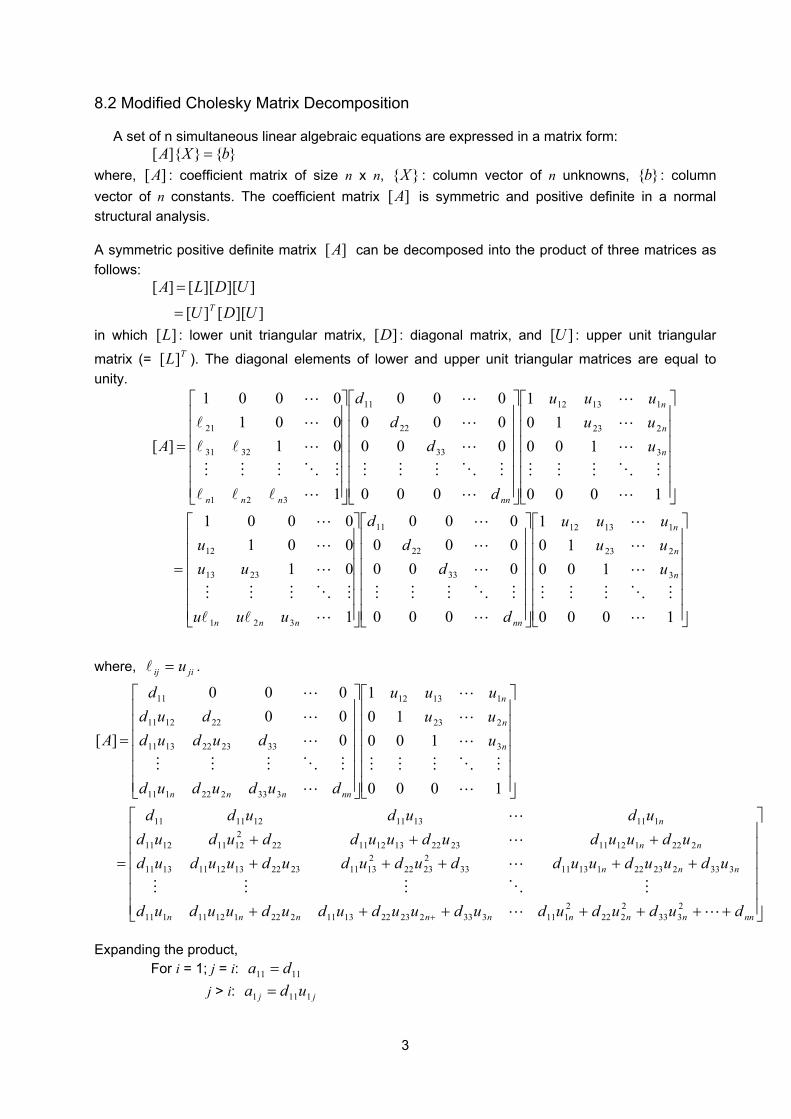
3

8.2 Modified Cholesky Matrix Decomposition

A set of n simultaneous linear algebraic equations are expressed in a matrix form: }{}]{[ bXA = where, ][A : coefficient matrix of size n x n, }{X : column vector of n unknowns, }{b : column vector of n constants. The coefficient matrix ][A is symmetric and positive definite in a normal structural analysis. A symmetric positive definite matrix ][A can be decomposed into the product of three matrices as follows:

]][[][

]][][[][UDU

UDLAT=

=

in which ][L : lower unit triangular matrix, ][D : diagonal matrix, and ][U : upper unit triangular

matrix (= TL][ ). The diagonal elements of lower and upper unit triangular matrices are equal to unity.

=

=

1000

10010

1

000

000000000

1

010010001

1000

10010

1

000

000000000

1

010010001

][

3

223

11312

33

22

11

321

2313

12

3

223

11312

33

22

11

321

3231

21

L

MOMMM

L

L

L

L

MOMMM

L

L

L

Lll

MOMMM

L

L

L

L

MOMMM

L

L

L

L

MOMMM

L

L

L

Llll

MOMMM

Lll

Ll

L

n

n

n

nnnnn

n

n

n

nnnnn

uuuuuu

d

dd

d

uuu

uuu

uuuuuu

d

dd

d

A

where, jiij u=l .

+++++++

++++++++

=

=

+ nnnnnnnnnn

nnn

nn

n

n

n

n

nnnnn

dududududuudududuudud

uduuduuddudududuudududuududuuddudud

udududd

uuuuuu

dududud

dududdud

d

A

LL

MOMMM

L

L

L

L

MOMMM

L

L

L

L

MOMMM

L

L

L

2333

2222

211133322322131122211211111

33322322113113322322

2131123221312111311

22211211232213121122212111211

1111311121111

3

223

11312

333222111

3323221311

221211

11

1000

10010

1

000000

][

Expanding the product, For i = 1; j = i: 1111 da = j > i: jj uda 1111 =

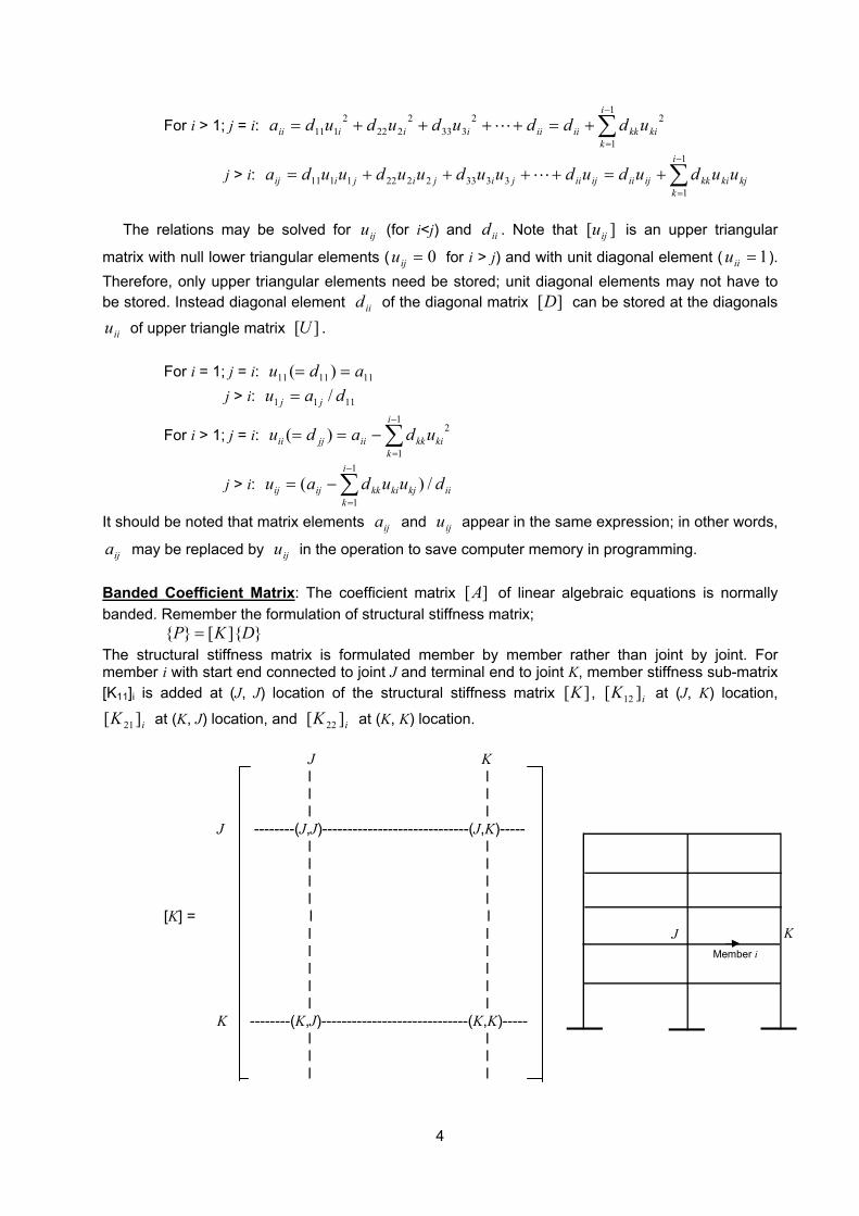
4

For i > 1; j = i: 21

1

2333

2222

2111 ki

i

kkkiiiiiiiii udddudududa ∑

−

=

+=++++= L

j > i: ∑−

=

+=++++=1

1333322221111

i

kkjkikkijiiijiijijijiij uudududuuduuduuda L

The relations may be solved for iju (for i<j) and iid . Note that ][ iju is an upper triangular

matrix with null lower triangular elements ( 0=iju for i > j) and with unit diagonal element ( 1=iiu ). Therefore, only upper triangular elements need be stored; unit diagonal elements may not have to be stored. Instead diagonal element iid of the diagonal matrix ][D can be stored at the diagonals

iiu of upper triangle matrix ][U .

For i = 1; j = i: 111111 )( adu == j > i: 1111 / dau jj =

For i > 1; j = i: ∑−

=

−==1

1

2)(i

kkikkiijjii udadu

j > i: iikjki

i

kkkijij duudau /)(

1

1∑−

=

−=

It should be noted that matrix elements ija and iju appear in the same expression; in other words,

ija may be replaced by iju in the operation to save computer memory in programming. Banded Coefficient Matrix: The coefficient matrix ][A of linear algebraic equations is normally banded. Remember the formulation of structural stiffness matrix; }]{[}{ DKP = The structural stiffness matrix is formulated member by member rather than joint by joint. For member i with start end connected to joint J and terminal end to joint K, member stiffness sub-matrix [K11]i is added at (J, J) location of the structural stiffness matrix ][K , iK ][ 12 at (J, K) location,

iK ][ 21 at (K, J) location, and iK ][ 22 at (K, K) location. J K l l l l l l J --------(J,J)-----------------------------(J,K)----- l l l l l l l l [K] = l l l l l l l l l l l l K --------(K,J)-----------------------------(K,K)----- l l l l l l

J KMember i

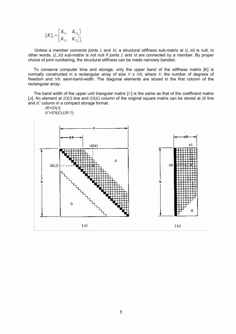
5

11 12

21 22

[ ]ii

K KK

K K

=

Unless a member connects joints L and M, a structural stiffness sub-matrix at (L,M) is null; in

other words, (L,M) sub-matrix is not null if joints L and M are connected by a member. By proper choice of joint numbering, the structural stiffness can be made narrowly banded.

To conserve computer time and storage, only the upper band of the stiffness matrix [K] is normally constructed in a rectangular array of size N x NB, where N: the number of degrees of freedom and NB: semi-band-width. The diagonal elements are stored in the first column of the rectangular array.

The band width of the upper unit triangular matrix [U] is the same as that of the coefficient matrix [A]. An element at ID(J) line and ID(K) column of the original square matrix can be stored at IR line and IC column in a compact storage format. IR=ID(J) IC=ID(K)-(IR-1)

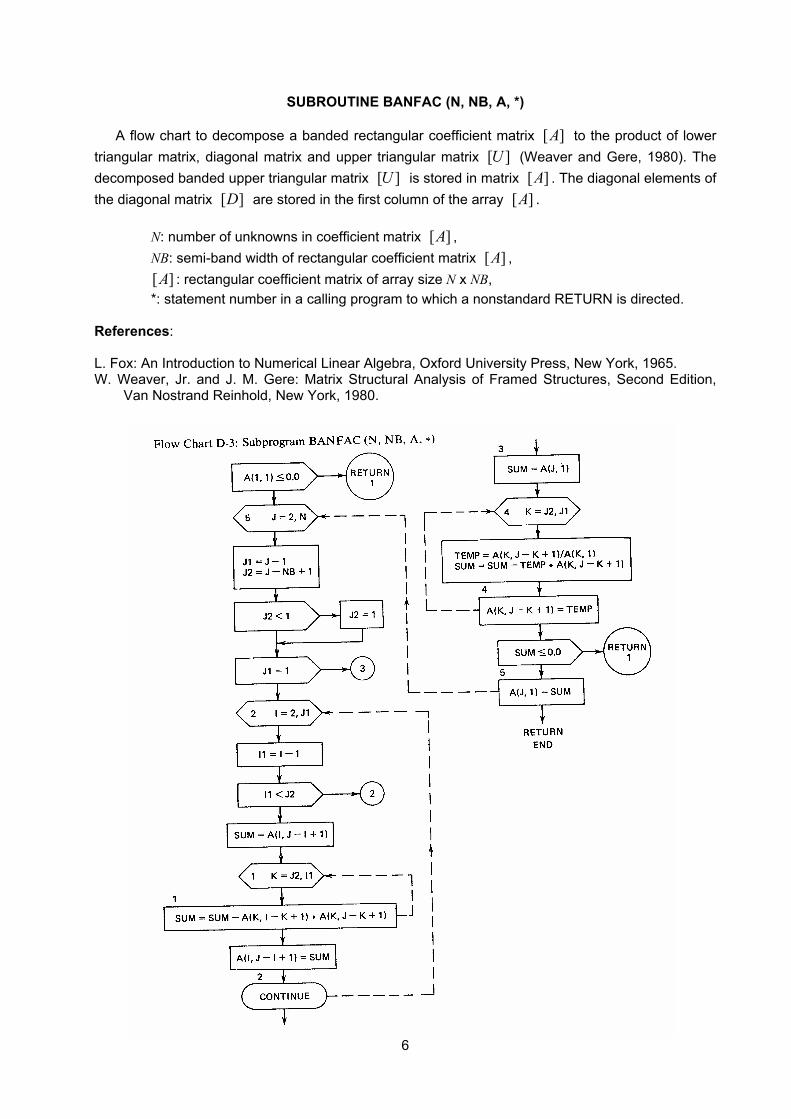
6

SUBROUTINE BANFAC (N, NB, A, *)

A flow chart to decompose a banded rectangular coefficient matrix ][A to the product of lower triangular matrix, diagonal matrix and upper triangular matrix ][U (Weaver and Gere, 1980). The decomposed banded upper triangular matrix ][U is stored in matrix ][A . The diagonal elements of the diagonal matrix ][D are stored in the first column of the array ][A .

N: number of unknowns in coefficient matrix ][A , NB: semi-band width of rectangular coefficient matrix ][A ,

][A : rectangular coefficient matrix of array size N x NB, *: statement number in a calling program to which a nonstandard RETURN is directed.

References: L. Fox: An Introduction to Numerical Linear Algebra, Oxford University Press, New York, 1965. W. Weaver, Jr. and J. M. Gere: Matrix Structural Analysis of Framed Structures, Second Edition,

Van Nostrand Reinhold, New York, 1980.

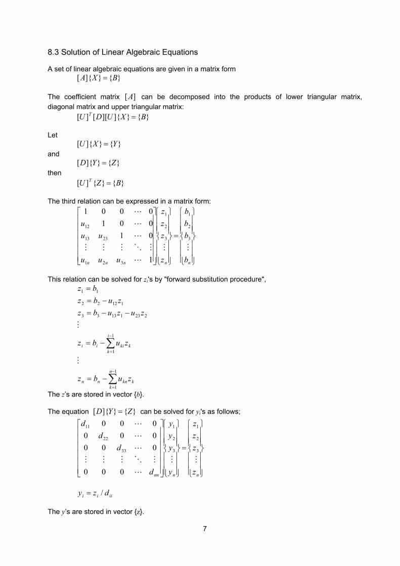
7

8.3 Solution of Linear Algebraic Equations A set of linear algebraic equations are given in a matrix form

}{}]{[ BXA = The coefficient matrix ][A can be decomposed into the products of lower triangular matrix, diagonal matrix and upper triangular matrix:

}{}]{][[][ BXUDU T = Let

}{}]{[ YXU = and }{}]{[ ZYD = then }{}{][ BZU T = The third relation can be expressed in a matrix form:

=

nnnnn b

bbb

z

zzz

uuu

uuu

MM

L

MOMMM

L

L

L

3

2

1

3

2

1

321

2313

12

1

010010001

This relation can be solved for zi's by "forward substitution procedure",

∑

∑

−

=

−

=

−=

−=

−−=−=

=

1

1

1

1

22311333

11222

11

n

kkknnn

i

kkkiii

zubz

zubz

zuzubzzubz

bz

M

M

The z’s are stored in vector {b}. The equation }{}]{[ ZYD = can be solved for yi's as follows;

=

nnnn z

zzz

y

yyy

d

dd

d

MM

L

MOMMM

L

L

L

3

2

1

3

2

1

33

22

11

000

000000000

iiii dzy /= The y’s are stored in vector {z}.

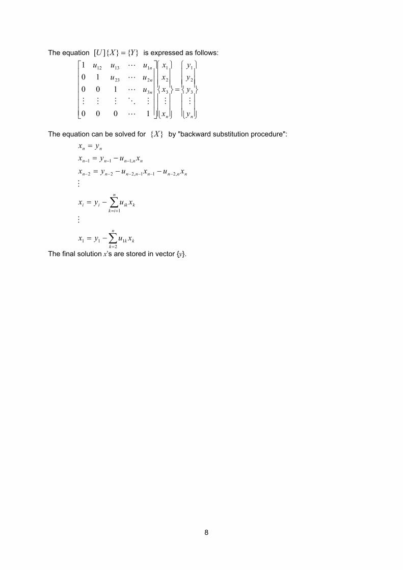
8

The equation }{}]{[ YXU = is expressed as follows:

=

nn

n

n

n

y

yyy

x

xxx

uuuuuu

MM

L

MOMMM

L

L

L

3

2

1

3

2

1

3

223

11312

1000

10010

1

The equation can be solved for }{X by "backward substitution procedure":

∑

∑

=

+=

−−−−−−

−−−

−=

−=

−−=

−==

n

kkk

n

ikkikii

nnnnnnnn

nnnnn

nn

xuyx

xuyx

xuxuyxxuyx

yx

2111

1

,211,222

,111

M

M

The final solution x’s are stored in vector {y}.

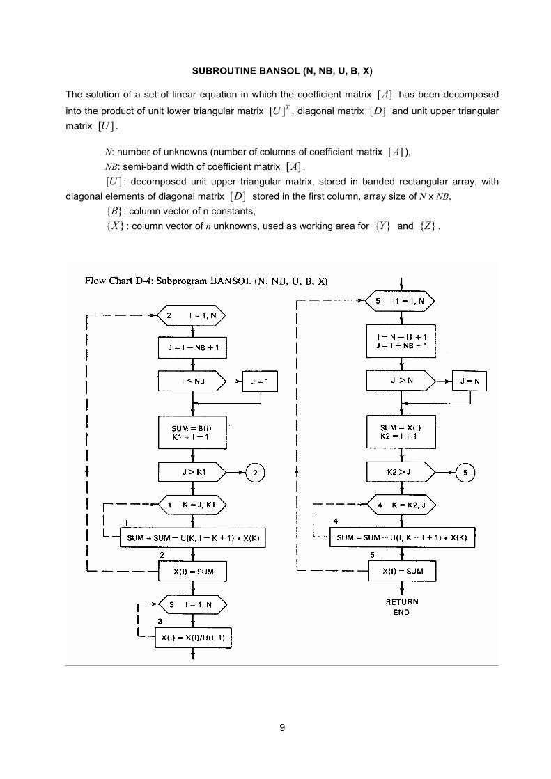
9

SUBROUTINE BANSOL (N, NB, U, B, X) The solution of a set of linear equation in which the coefficient matrix ][A has been decomposed

into the product of unit lower triangular matrix TU ][ , diagonal matrix ][D and unit upper triangular matrix ][U .

N: number of unknowns (number of columns of coefficient matrix ][A ), NB: semi-band width of coefficient matrix ][A ,

][U : decomposed unit upper triangular matrix, stored in banded rectangular array, with diagonal elements of diagonal matrix ][D stored in the first column, array size of N x NB,

}{B : column vector of n constants, }{X : column vector of n unknowns, used as working area for }{Y and }{Z .

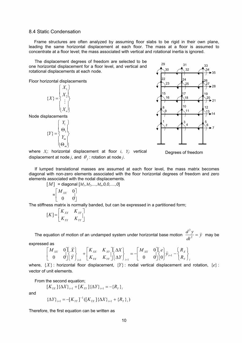
10

8.4 Static Condensation

Frame structures are often analyzed by assuming floor slabs to be rigid in their own plane, leading the same horizontal displacement at each floor. The mass at a floor is assumed to concentrate at a floor level; the mass associated with vertical and rotational inertia is ignored.

The displacement degrees of freedom are selected to be one horizontal displacement for a floor level, and vertical and rotational displacements at each node. Floor horizontal displacements

1

2{ }

n

XX

X

X

=

M

Node displacements

1

1{ }m

m

Y

YY

Θ = Θ

where Xi: horizontal displacement at floor i, Yj: vertical displacement at node j, and jθ : rotation at node j.

If lumped translational masses are assumed at each floor level, the mass matrix becomes diagonal with non-zero elements associated with the floor horizontal degrees of freedom and zero elements associated with the nodal displacements. ][M = diagonal [M1,M2,...,Mn,0,0,....,0]

=

000XXM

The stiffness matrix is normally banded, but can be expressed in a partitioned form;

=

YYYX

XYXX

KKKK

K ][

The equation of motion of an undamped system under horizontal base motion ydt

yd&&=2

2

may be

expressed as

iY

Xi

XX

iYYYX

XYXX

i

XX

RR

yeM

YX

KKKK

YXM

−

−=

∆∆

+

+

++

111

0000

000

&&&&

&&

where, }{X : horizontal floor displacement, }{Y : nodal vertical displacement and rotation, }{e : vector of unit elements.

From the second equation; iYiYYiYX RYKXK }{}]{[}]{[ 11 −=∆+∆ ++

and )}{}]{([][}{ 1

11 iYiYXYYi RXKKY +∆−=∆ +

−+

Therefore, the first equation can be written as

12

3 4

56

7

89

10 11

1213

14

1516

17 18

1920

21

2223

24 25

2627

28

29

3031

32 3334

35

Degrees of freedom

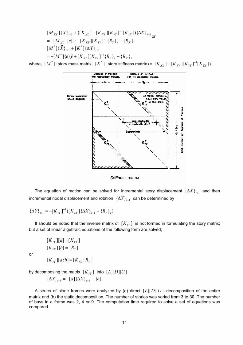
11

iXiYYYKYXX

iYXYYXYXXiXX

RRKKyeM

XKKKKXM

}{}{]][[}]{[

}]){[]][[]([}]{[1

11

1

−+−=

∆−+−

+−

+

&&

&&or

iXiYYYXY

ii

RRKKyeM

XKXM

}{}{]][[}]{[

}]{[}]{[1*

1*

1*

−+−=

∆+−

++

&&

&&

where, ][ *M : story mass matrix, ][ *K : story stiffness matrix (= ][]][[][ 1YXYYXYXX KKKK −− ).

The equation of motion can be solved for incremental story displacement 1}{ +∆ iX and then

incremental nodal displacement and rotation 1}{ +∆ iY can be determined by

)}{}]{([][}{ 11

1 iYiYXYYi RXKKY +∆−=∆ +−

+

It should be noted that the inverse matrix of ][ YYK is not formed in formulating the story matrix; but a set of linear algebraic equations of the following form are solved;

}{}]{[][]][[

YYY

YXYY

RbKKaK

==

or ][]][[ YYXYY RKbaK MM =

by decomposing the matrix ][ YYK into ]][][[ UDL . }{}]{[}{ 11 bXaY ii −∆−=∆ ++

A series of plane frames were analyzed by (a) direct ]][][[ UDL decomposition of the entire matrix and (b) the static decomposition. The number of stories was varied from 3 to 30. The number of bays in a frame was 2, 4 or 9. The computation time required to solve a set of equations was compared.

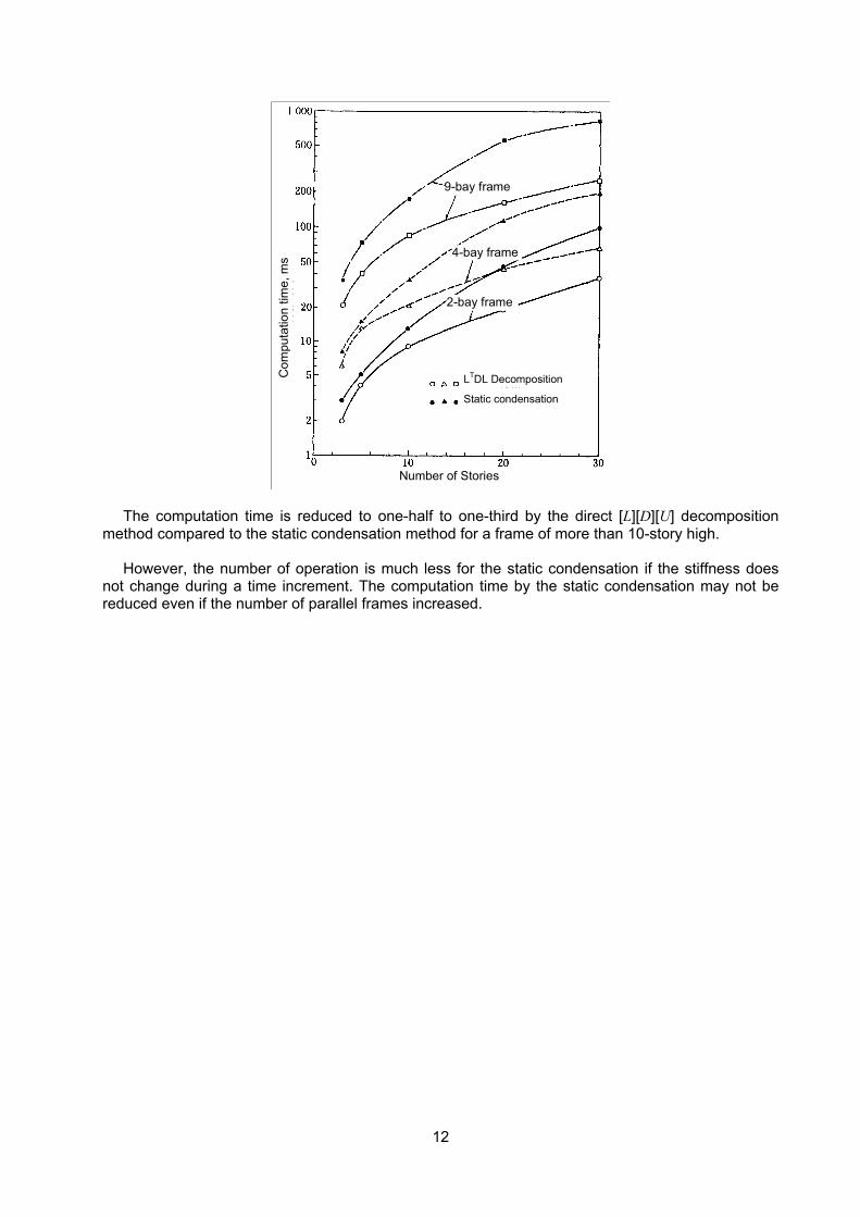
12

Number of Stories

Com

puta

tion

time,

ms

9-bay frame

4-bay frame

2-bay frame

LTDL Decomposition

Static condensation

The computation time is reduced to one-half to one-third by the direct [L][D][U] decomposition method compared to the static condensation method for a frame of more than 10-story high.

However, the number of operation is much less for the static condensation if the stiffness does not change during a time increment. The computation time by the static condensation may not be reduced even if the number of parallel frames increased.

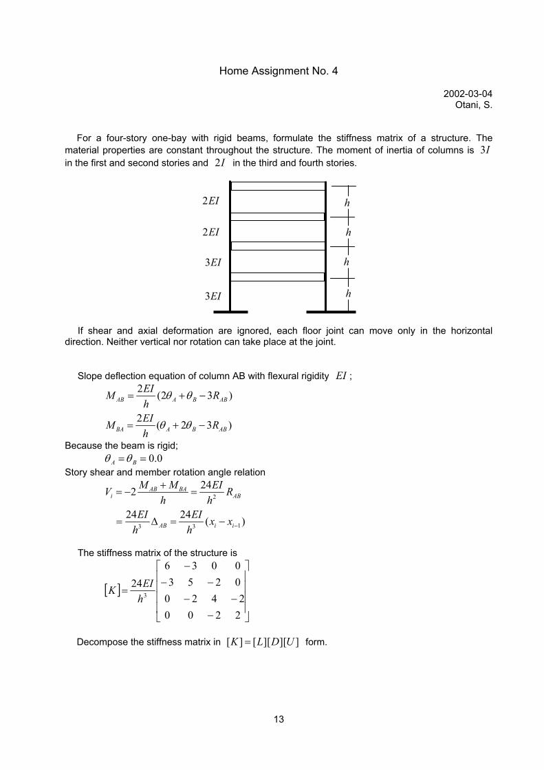
13

Home Assignment No. 4

2002-03-04 Otani, S.

For a four-story one-bay with rigid beams, formulate the stiffness matrix of a structure. The material properties are constant throughout the structure. The moment of inertia of columns is 3I in the first and second stories and 2I in the third and fourth stories.

h

h

h

h3EI

3EI

2EI

2EI

If shear and axial deformation are ignored, each floor joint can move only in the horizontal direction. Neither vertical nor rotation can take place at the joint.

Slope deflection equation of column AB with flexural rigidity EI ;

2 (2 3 )

2 ( 2 3 )

AB A B AB

BA A B AB

EIM RhEIM Rh

θ θ

θ θ

= + −

= + −

Because the beam is rigid; 0.0A Bθ θ= = Story shear and member rotation angle relation

2

13 3

242

24 24 ( )

AB BAi AB

AB i i

M M EIV Rh h

EI EI x xh h −

+= − =

= ∆ = −

The stiffness matrix of the structure is

[ ]

−−−

−−−

=

22002420

02530036

243hEIK

Decompose the stiffness matrix in [ ] [ ][ ][ ]K L D U= form.

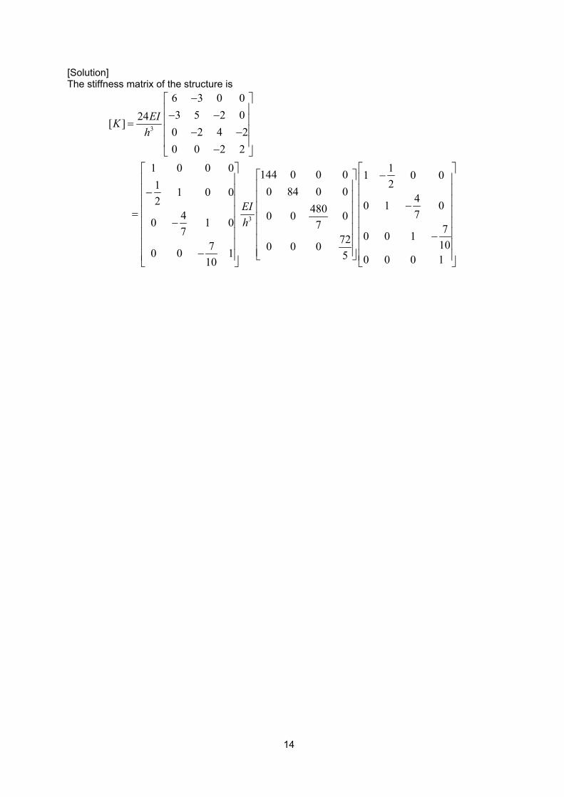
14

[Solution] The stiffness matrix of the structure is

3

3

6 3 0 03 5 2 024[ ]

0 2 4 20 0 2 2

1 0 0 0 1144 0 0 0 1 0 021 0 84 0 01 0 0 42 0 1 0480 74 0 0 00 1 0 7 77 0 0 172 107 0 0 00 0 1 5 0 0 0 110

EIKh

EIh

− − − = − − −

− − − = − − −

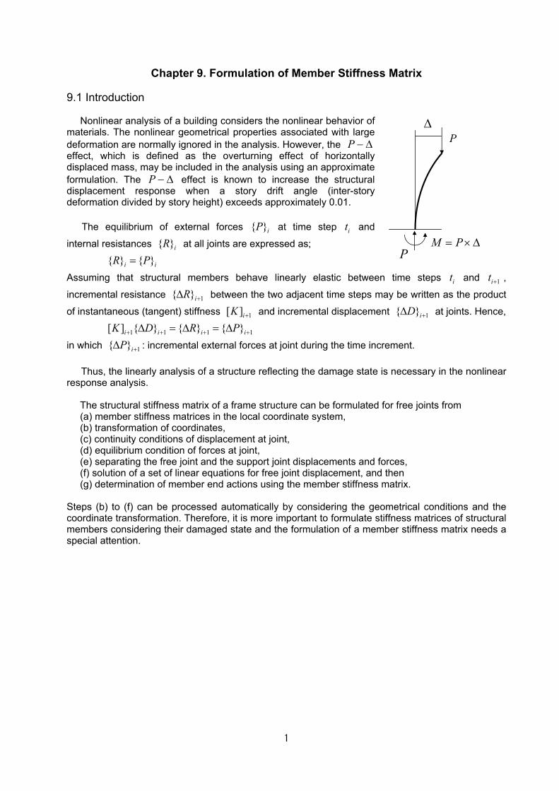
1

Chapter 9. Formulation of Member Stiffness Matrix 9.1 Introduction

Nonlinear analysis of a building considers the nonlinear behavior of materials. The nonlinear geometrical properties associated with large deformation are normally ignored in the analysis. However, the ∆−P effect, which is defined as the overturning effect of horizontally displaced mass, may be included in the analysis using an approximate formulation. The ∆−P effect is known to increase the structural displacement response when a story drift angle (inter-story deformation divided by story height) exceeds approximately 0.01.

The equilibrium of external forces { }iP at time step it and

internal resistances { }iR at all joints are expressed as;

{ } { }i iR P=

Assuming that structural members behave linearly elastic between time steps it and 1it + ,

incremental resistance 1{ }iR +∆ between the two adjacent time steps may be written as the product

of instantaneous (tangent) stiffness 1[ ]iK + and incremental displacement 1{ }iD +∆ at joints. Hence,

1 1 1 1[ ] { } { } { }i i i iK D R P+ + + +∆ = ∆ = ∆

in which 1{ }iP +∆ : incremental external forces at joint during the time increment.

Thus, the linearly analysis of a structure reflecting the damage state is necessary in the nonlinear response analysis.

The structural stiffness matrix of a frame structure can be formulated for free joints from (a) member stiffness matrices in the local coordinate system, (b) transformation of coordinates, (c) continuity conditions of displacement at joint, (d) equilibrium condition of forces at joint, (e) separating the free joint and the support joint displacements and forces, (f) solution of a set of linear equations for free joint displacement, and then (g) determination of member end actions using the member stiffness matrix.

Steps (b) to (f) can be processed automatically by considering the geometrical conditions and the coordinate transformation. Therefore, it is more important to formulate stiffness matrices of structural members considering their damaged state and the formulation of a member stiffness matrix needs a special attention.

P

∆

P

M P= ×∆

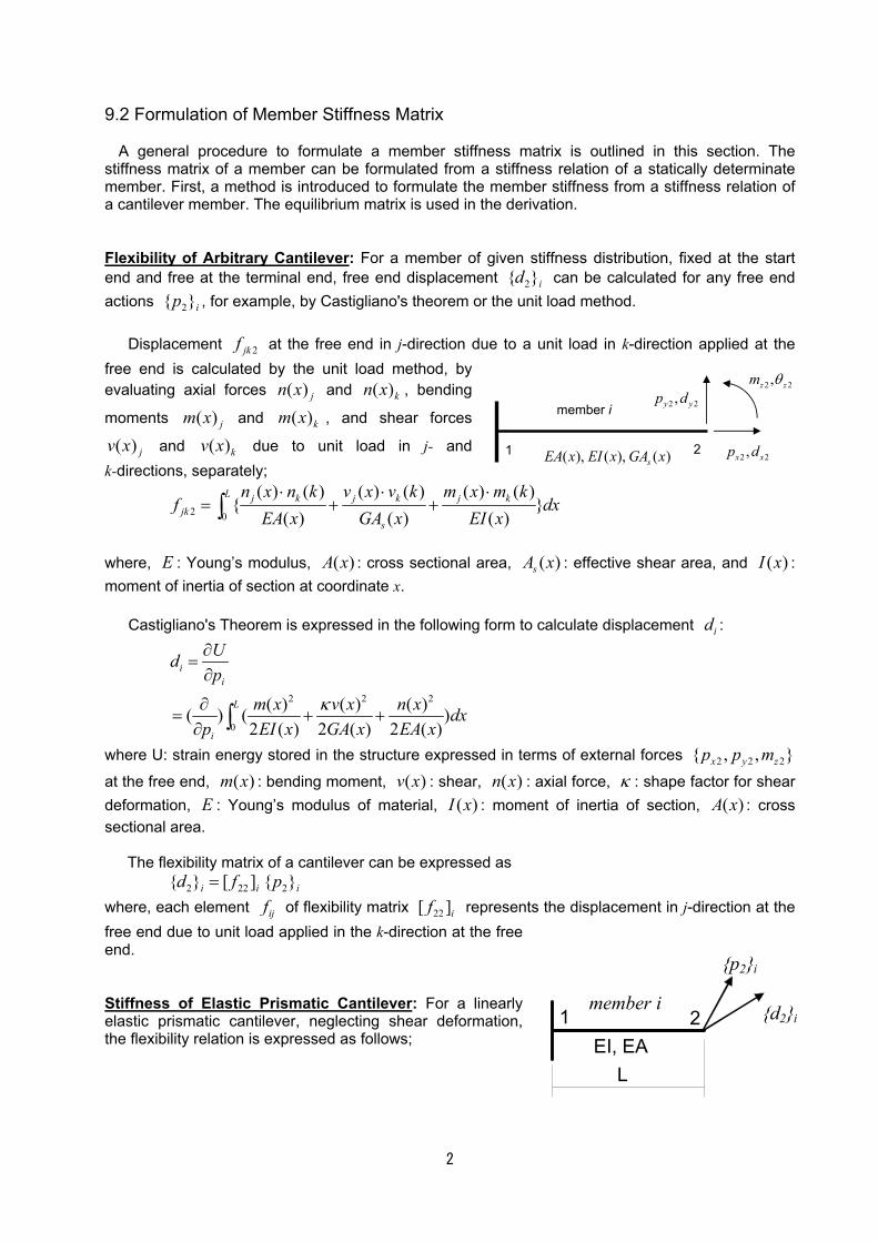
2

9.2 Formulation of Member Stiffness Matrix

A general procedure to formulate a member stiffness matrix is outlined in this section. The stiffness matrix of a member can be formulated from a stiffness relation of a statically determinate member. First, a method is introduced to formulate the member stiffness from a stiffness relation of a cantilever member. The equilibrium matrix is used in the derivation. Flexibility of Arbitrary Cantilever: For a member of given stiffness distribution, fixed at the start end and free at the terminal end, free end displacement { }d i2 can be calculated for any free end actions { }p i2 , for example, by Castigliano's theorem or the unit load method.

Displacement 2jkf at the free end in j-direction due to a unit load in k-direction applied at the free end is calculated by the unit load method, by evaluating axial forces ( ) jn x and ( )kn x , bending

moments ( ) jm x and ( )km x , and shear forces

( ) jv x and ( )kv x due to unit load in j- and k-directions, separately;

2 0

( ) ( ) ( ) ( ) ( ) ( ){ }

( ) ( ) ( )L j k j k j k

jks

n x n k v x v k m x m kf dx

EA x GA x EI x⋅ ⋅ ⋅

= + +∫

where, E : Young’s modulus, ( )A x : cross sectional area, ( )sA x : effective shear area, and ( )I x : moment of inertia of section at coordinate x.

Castigliano's Theorem is expressed in the following form to calculate displacement id :

2 2 2

0

( ) ( ) ( )( ) ( )2 ( ) 2 ( ) 2 ( )

ii

L

i

Udp

m x v x n x dxp EI x GA x EA x

κ

∂=∂

∂= + +

∂ ∫

where U: strain energy stored in the structure expressed in terms of external forces 2 2 2{ , , }x y zp p m

at the free end, ( )m x : bending moment, ( )v x : shear, ( )n x : axial force, κ : shape factor for shear deformation, E : Young’s modulus of material, ( )I x : moment of inertia of section, ( )A x : cross sectional area.

The flexibility matrix of a cantilever can be expressed as { } [ ] { }d f pi i i2 22 2= where, each element ijf of flexibility matrix 22[ ]if represents the displacement in j-direction at the free end due to unit load applied in the k-direction at the free end. Stiffness of Elastic Prismatic Cantilever: For a linearly elastic prismatic cantilever, neglecting shear deformation, the flexibility relation is expressed as follows;

1 2

{p2}i

{d2}i

EI, EA

member i

L

2 2,x xp d

2 2,y yp d 2 2,z zm θ

member i

( ), ( ), ( )sEA x EI x GA x 1 2

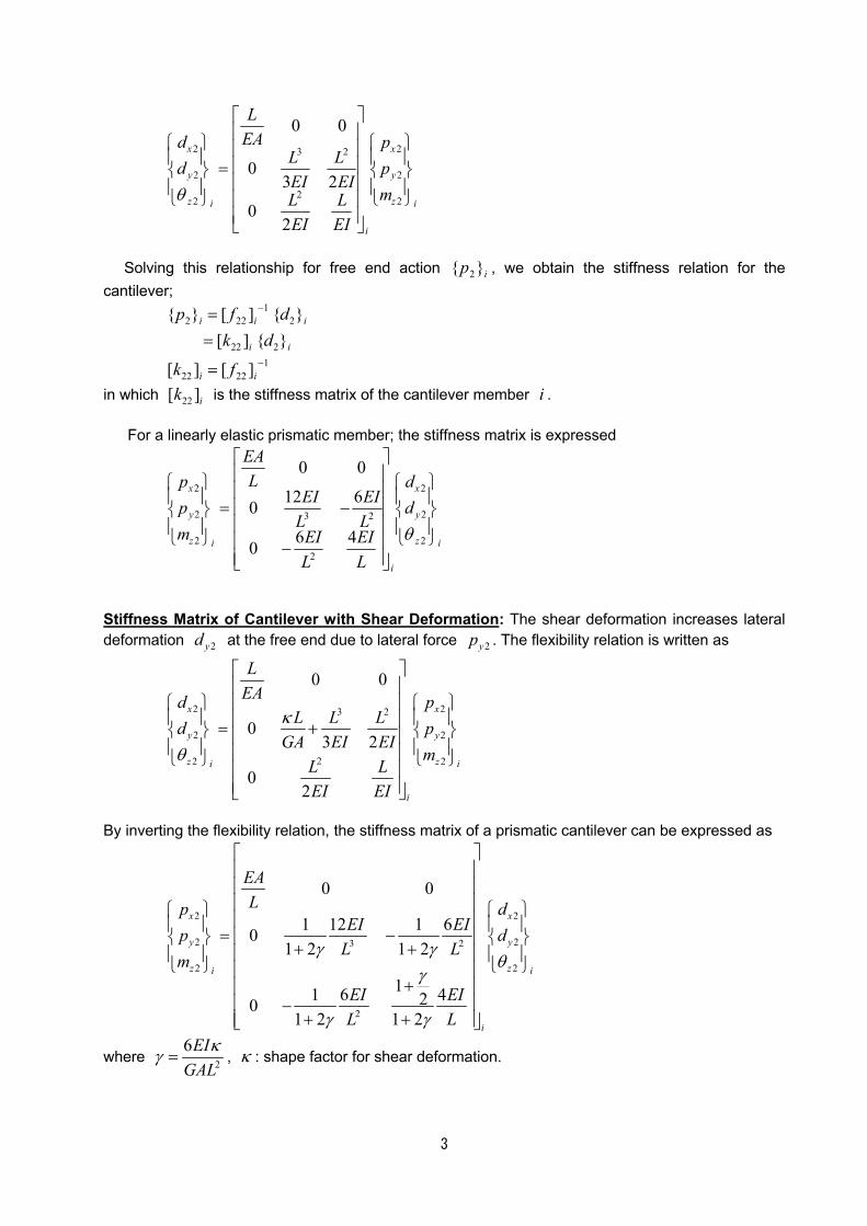
3

dd

LEA

LEI

LEI

LEI

LEI

ppm

x

y

z i

i

x

y

z i

2

2

2

3 2

2

2

2

2

0 0

03 2

02

θ

=

Solving this relationship for free end action ip }{ 2 , we obtain the stiffness relation for the

cantilever;

{ } [ ] { }

[ ] { }p f d

k di i i

i i

2 221

2

22 2

==

−

[ ] [ ]k fi i22 221= −

in which 22[ ]ik is the stiffness matrix of the cantilever member i .

For a linearly elastic prismatic member; the stiffness matrix is expressed

ppm

EAL

EIL

EIL

EIL

EIL

dd

x

y

z i

i

x

y

z i

2

2

2

3 2

2

2

2

2

0 0

0 12 6

0 6 4

= −

−

θ

Stiffness Matrix of Cantilever with Shear Deformation: The shear deformation increases lateral deformation 2yd at the free end due to lateral force 2yp . The flexibility relation is written as

2 23 2

2 2

22 2

0 0

03 2

02

x x

y y

z zi i

i

LEAd p

L L Ld pGA EI EI

mL LEI EI

κ

θ

= +

By inverting the flexibility relation, the stiffness matrix of a prismatic cantilever can be expressed as

2 2

2 23 2

2 2

2

0 0

1 12 1 601 2 1 2

11 6 4201 2 1 2

x x

y y

z zi i

i

EALp d

EI EIp dL L

m

EI EIL L

γ γθ

γ

γ γ

= − + +

+

−+ +

where 2

6EIGAL

κγ = , κ : shape factor for shear deformation.

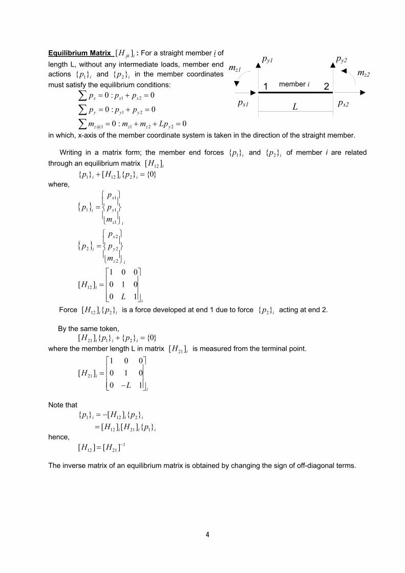
4

Equilibrium Matrix [ ]H jk i : For a straight member i of length L, without any intermediate loads, member end actions ip }{ 1 and ip }{ 2 in the member coordinates must satisfy the equilibrium conditions:

1 2

1 2

@1 1 2 2

0 : 0

0 : 0

0 : 0

x x x

y y y

z z z y

p p p

p p p

m m m Lp

= + =

= + =

= + + =

∑∑∑

in which, x-axis of the member coordinate system is taken in the direction of the straight member.

Writing in a matrix form; the member end forces { }p i1 and { }p i2 of member i are related through an equilibrium matrix [ ]H i12 { } [ ] { } { }p H pi i i1 12 2 0+ = where,

{ }

{ }iz

y

x

i

iz

y

x

i

mpp

p

mpp

p

=

=

2

2

2

2

1

1

1

1

[ ]HL

i

i

12

1 0 00 1 00 1

=

Force 12 2[ ] { }i iH p is a force developed at end 1 due to force 2{ }ip acting at end 2.

By the same token, [ ] { } { } { }H p pi i i21 1 2 0+ = where the member length L in matrix [ ]H i21 is measured from the terminal point.

[ ]HL

i

i

21

1 0 00 1 00 1

=−

Note that

{ } [ ] { }

[ ] [ ] { }p H p

H H pi i i

i i i

1 12 2

12 21 1

= −=

hence, [ ] [ ]H H12 21

1= − The inverse matrix of an equilibrium matrix is obtained by changing the sign of off-diagonal terms.

py1 py2

px1 px2

mz1 mz2

L

1 2member i

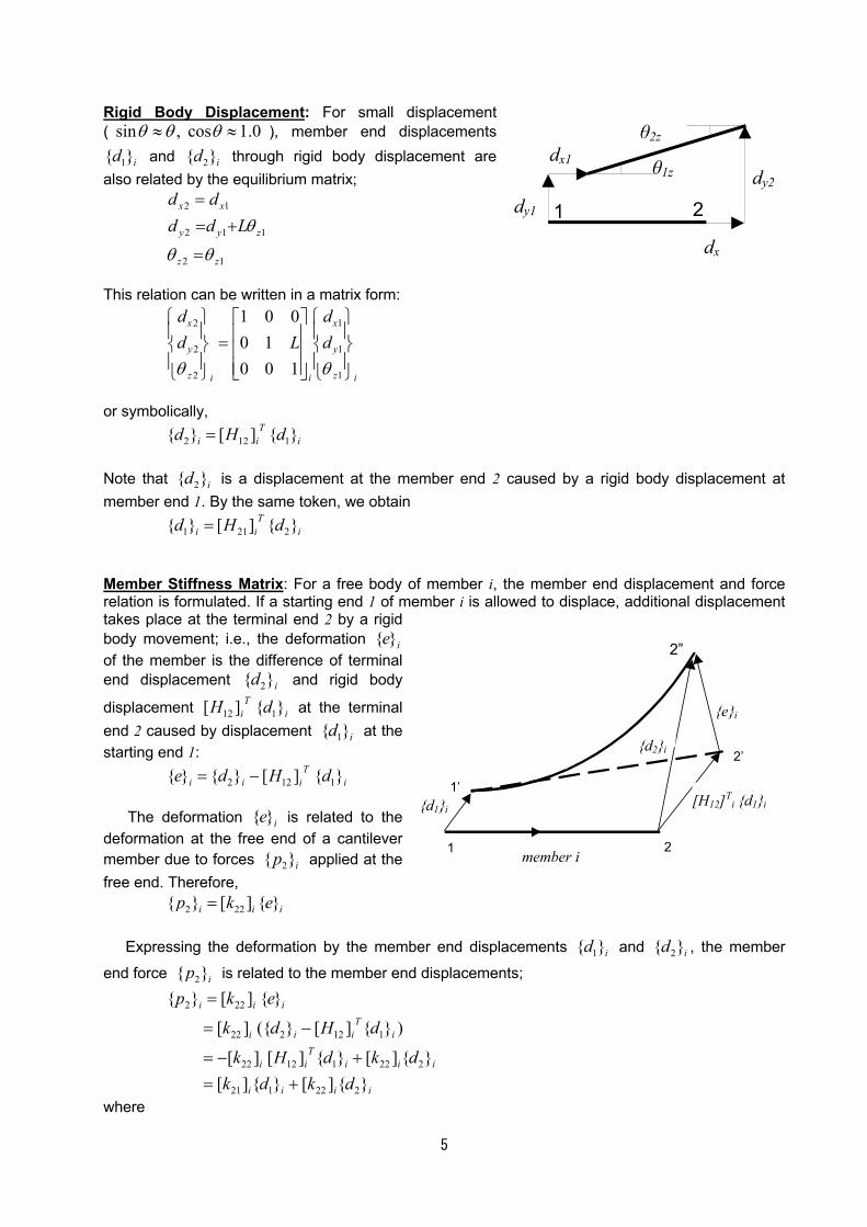
5

Rigid Body Displacement: For small displacement ( sin , cos 1.0θ θ θ≈ ≈ ), member end displacements

1{ }id and 2{ }id through rigid body displacement are also related by the equilibrium matrix;

12

112

12

zz

zyy

xx

Ldddd

θθ

θ

=

+==

This relation can be written in a matrix form:

dd L

dd

x

y

z i i

x

y

z i

2

2

2

1

1

1

1 0 00 10 0 1θ θ

=

or symbolically, 2 12 1{ } [ ] { }T

i i id H d= Note that 2{ }id is a displacement at the member end 2 caused by a rigid body displacement at member end 1. By the same token, we obtain 1 21 2{ } [ ] { }T

i i id H d= Member Stiffness Matrix: For a free body of member i, the member end displacement and force relation is formulated. If a starting end 1 of member i is allowed to displace, additional displacement takes place at the terminal end 2 by a rigid body movement; i.e., the deformation { }e i of the member is the difference of terminal end displacement { }d i2 and rigid body

displacement [ ] { }H diT

i12 1 at the terminal end 2 caused by displacement { }d i1 at the starting end 1: { } { } [ ] { }e d H di i i

Ti= −2 12 1

The deformation { }e i is related to the

deformation at the free end of a cantilever member due to forces 2{ }ip applied at the free end. Therefore, 2 22{ } [ ] { }i i ip k e=

Expressing the deformation by the member end displacements 1{ }id and 2{ }id , the member

end force 2{ }ip is related to the member end displacements;

{ } [ ] { }

[ ] ({ } [ ] { } )

[ ] [ ] { } [ ] { }[ ] { } [ ] { }

p k e

k d H d

k H d k dk d k d

i i i

i i iT

i

i iT

i i i

i i i i

2 22

22 2 12 1

22 12 1 22 2

21 1 22 2

=

= −

= − += +

where

dy1

dy2

dx1

dx

θ1z

θ2z

1 2

1 2

{d1}i

{e}i

2’

1’

{d2}i

2”

[H12]Ti {d1}i

member i

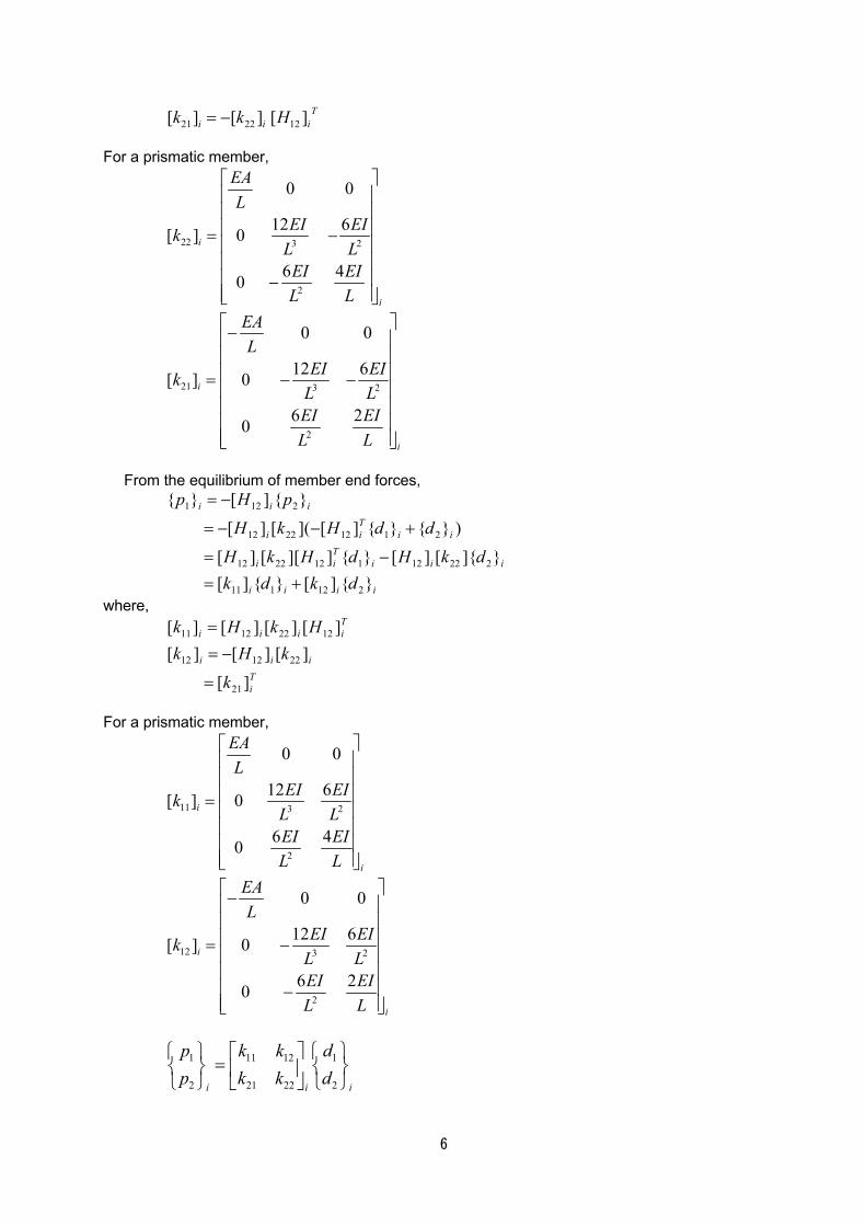
6

[ ] [ ] [ ]k k Hi i iT

21 22 12= − For a prismatic member,

22 3 2

2

0 0

12 6[ ] 0

6 40

i

i

EAL

EI EIkL LEI EIL L

= − −

21 3 2

2

0 0

12 6[ ] 0

6 20

i

i

EAL

EI EIkL LEI EIL L

− = − −

From the equilibrium of member end forces,

iiii

iiiTii

iiTii

iii

dkdkdkHdHkH

ddHkH

pHp

}{][}{][}]{[][}{]][[][

)}{}{][]([][

}{][}{

212111

222121122212

21122212

2121

+=−=

+−−=

−=

where,

Ti

iii

Tiiii

k

kHkHkHk

][

][][][][][][][

21

221212

12221211

=

−==

For a prismatic member,

11 3 2

2

0 0

12 6[ ] 0

6 40

i

i

EAL

EI EIkL LEI EIL L

=

12 3 2

2

0 0

12 6[ ] 0

6 20

i

i

EAL

EI EIkL LEI EIL L

− = − −

1 11 12 1

2 21 22 2i i i

p k k dp k k d

=

7

------------------------------ Note: TTT ABBA ][][])][([ =

8

9.3 Member with Rigid Ends It is often necessary to consider rigid zones at member ends. For example, a beam-column connection may be assumed to be rigid or a structural wall is represented by a column with rigid beams at each floor. Let us consider the treatment of a member having rigid zones at the ends.

Beam-column Connection Structural Wall Equilibrium Matrix: The equilibrium matrix ][ ABH for member AB, not lying in x-direction, can be defined in a more general form if the lengths of the member are ABx and ABy in x- and y-direction, respectively;

@

0 : 0

0 : 0

0 : 0

x xA xB

y yA yB

z A zA zB xB AB yB AB

p p p

p p p

m m m p y p x

= + =

= + =

= + − + =

∑∑∑

{ } [ ]{ } {0}A AB Bp H p+ =

The equilibrium matrix for this member is given as

−=

1010001

][

ABAB

AB

xyH

It should be noted that force { }Ap at starting end A is necessary to satisfy the equilibrium when

force { }Bp acts at the terminal end B. Product of Equilibrium Matrices: Consider regions AB and BC connected at B. No external force is assumed to act at joint B.

If force { }Cp acts at member end C of region BC, force { '}Bp at B end is necessary to satisfy the equilibrium in the region;

}]{[}'{

}0{}]{[}'{

CBCB

CBCB

pHppHp

−==+

The equilibrium of forces at end B is

}]{[}'{}{

}0{}'{}{

CBCBB

BB

pHpppp

=−==+

A

B

yAB

xAB x

y

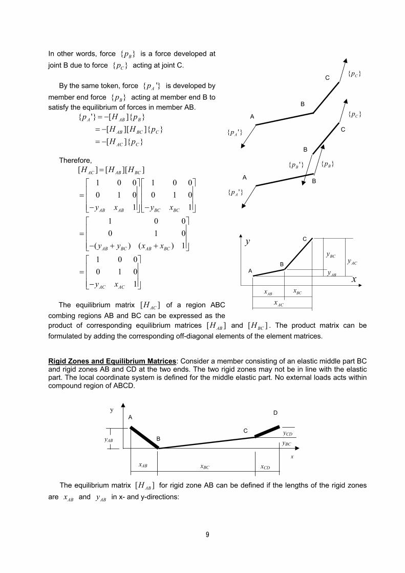
9

In other words, force { }Bp is a force developed at joint B due to force { }Cp acting at joint C.

By the same token, force { '}Ap is developed by member end force { }Bp acting at member end B to satisfy the equilibrium of forces in member AB.

}]{[}]{][[

}]{[}'{

CAC

CBCAB

BABA

pHpHH

pHp

−=−=−=

Therefore,

[ ] [ ][ ]1 0 0 1 0 00 1 0 0 1 0

1 1

1 0 00 1 0

( ) ( ) 1

1 0 00 1 0

1

AC AB BC

AB AB BC BC

AB BC AB BC

AC AC

H H H

y x y x

y y x x

y x

=

= − − = − + + = −

The equilibrium matrix [ ]ACH of a region ABC

combing regions AB and BC can be expressed as the product of corresponding equilibrium matrices [ ]ABH and [ ]BCH . The product matrix can be formulated by adding the corresponding off-diagonal elements of the element matrices. Rigid Zones and Equilibrium Matrices: Consider a member consisting of an elastic middle part BC and rigid zones AB and CD at the two ends. The two rigid zones may not be in line with the elastic part. The local coordinate system is defined for the middle elastic part. No external loads acts within compound region of ABCD.

The equilibrium matrix [ ]ABH for rigid zone AB can be defined if the lengths of the rigid zones are ABx and ABy in x- and y-directions:

A

B

C }{ Cp

}'{ Ap

A

}'{ Ap

}{ Cp

}'{ Bp }{ Bp

B

B

C

ABx BCx

BCy

ABy

ACx

ACy

x

y

AB

C

A

B C

D

xAB xBC xCD

yAB yCD

y

x

yBC

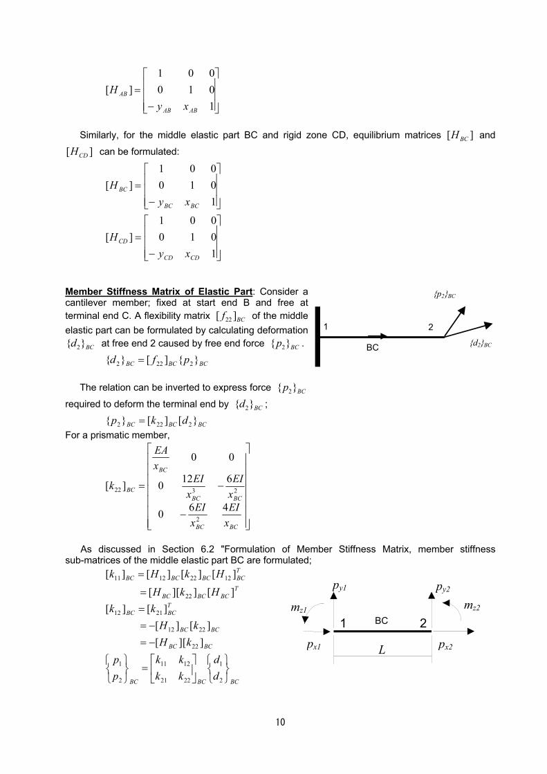
10

−=

1010001

][

ABAB

AB

xyH

Similarly, for the middle elastic part BC and rigid zone CD, equilibrium matrices [ ]BCH and

[ ]CDH can be formulated:

−=

−=

1010001

][

1010001

][

CDCD

CD

BCBC

BC

xyH

xyH

Member Stiffness Matrix of Elastic Part: Consider a cantilever member; fixed at start end B and free at terminal end C. A flexibility matrix 22[ ]BCf of the middle elastic part can be formulated by calculating deformation

2{ }BCd at free end 2 caused by free end force 2{ }BCp .

BCBCBC pfd }{][}{ 2222 =

The relation can be inverted to express force 2{ }BCp

required to deform the terminal end by 2{ }BCd ;

BCBCBC dkp }[][}{ 2222 = For a prismatic member,

−

−=

BCBC

BCBC

BC

BC

xEI

xEI

xEI

xEI

xEA

k

460

6120

00

][

2

2322

As discussed in Section 6.2 "Formulation of Member Stiffness Matrix, member stiffness

sub-matrices of the middle elastic part BC are formulated;

T

BCBCBC

TBCBCBCBC

HkH

HkHk

][]][[

][][][][

22

12221211

=

=

BCBC

BCBC

TBCBC

kHkH

kk

]][[][][

][][

22

2212

2112

−=−=

=

BCBCBC d

dkkkk

pp

=

2

1

2221

1211

2

1

1 2

{p2}BC

{d2}BCBC

py1 py2

px1 px2

mz1 mz2

L

1 2BC

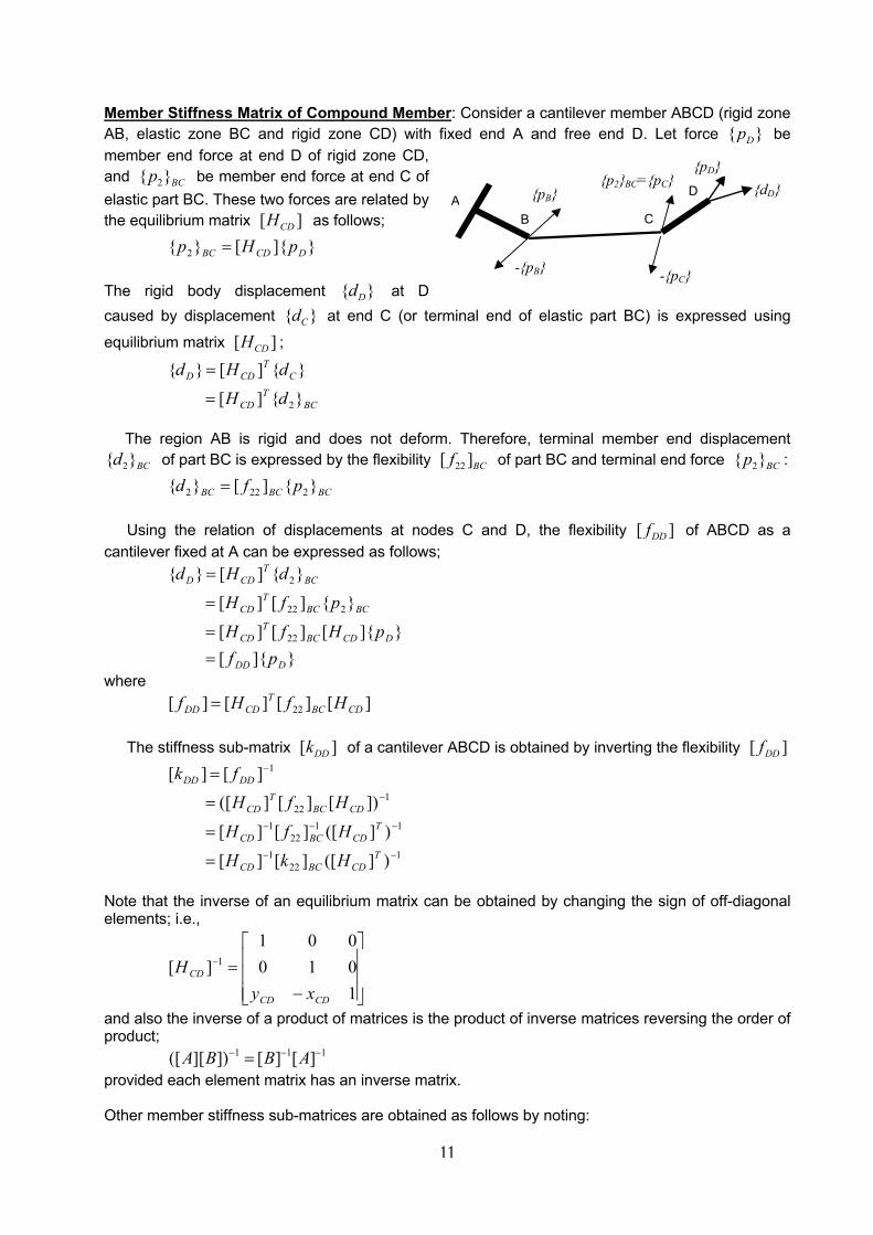
11

Member Stiffness Matrix of Compound Member: Consider a cantilever member ABCD (rigid zone AB, elastic zone BC and rigid zone CD) with fixed end A and free end D. Let force { }Dp be member end force at end D of rigid zone CD, and 2{ }BCp be member end force at end C of elastic part BC. These two forces are related by the equilibrium matrix [ ]CDH as follows;

}]{[}{ 2 DCDBC pHp = The rigid body displacement { }Dd at D caused by displacement { }Cd at end C (or terminal end of elastic part BC) is expressed using

equilibrium matrix [ ]CDH ;

BC

TCD

CT

CDD

dH

dHd

}{][

}{][}{

2=

=

The region AB is rigid and does not deform. Therefore, terminal member end displacement 2{ }BCd of part BC is expressed by the flexibility 22[ ]BCf of part BC and terminal end force 2{ }BCp :

BCBCBC pfd }{][}{ 2222 =

Using the relation of displacements at nodes C and D, the flexibility [ ]DDf of ABCD as a cantilever fixed at A can be expressed as follows;

}]{[}]{[][][

}{][][

}{][}{

22

222

2

DDD

DCDBCT

CD

BCBCT

CD

BCT

CDD

pfpHfH

pfH

dHd

==

=

=

where ][][][][ 22 CDBC

TCDDD HfHf =

The stiffness sub-matrix [ ]DDk of a cantilever ABCD is obtained by inverting the flexibility [ ]DDf

122

1

1122

1

122

1

)]([][][

)]([][][

])[][]([][][

−−

−−−

−

−

=

=

=

=

TCDBCCD

TCDBCCD

CDBCT

CD

DDDD

HkH

HfH

HfHfk

Note that the inverse of an equilibrium matrix can be obtained by changing the sign of off-diagonal elements; i.e.,

−=−

1010001

][ 1

CDCD

CD

xyH

and also the inverse of a product of matrices is the product of inverse matrices reversing the order of product; 1 1 1([ ][ ]) [ ] [ ]A B B A− − −= provided each element matrix has an inverse matrix. Other member stiffness sub-matrices are obtained as follows by noting:

A B C

D

{pD} {dD}{p2}BC={pC}

-{pC}

{pB}

-{pB}

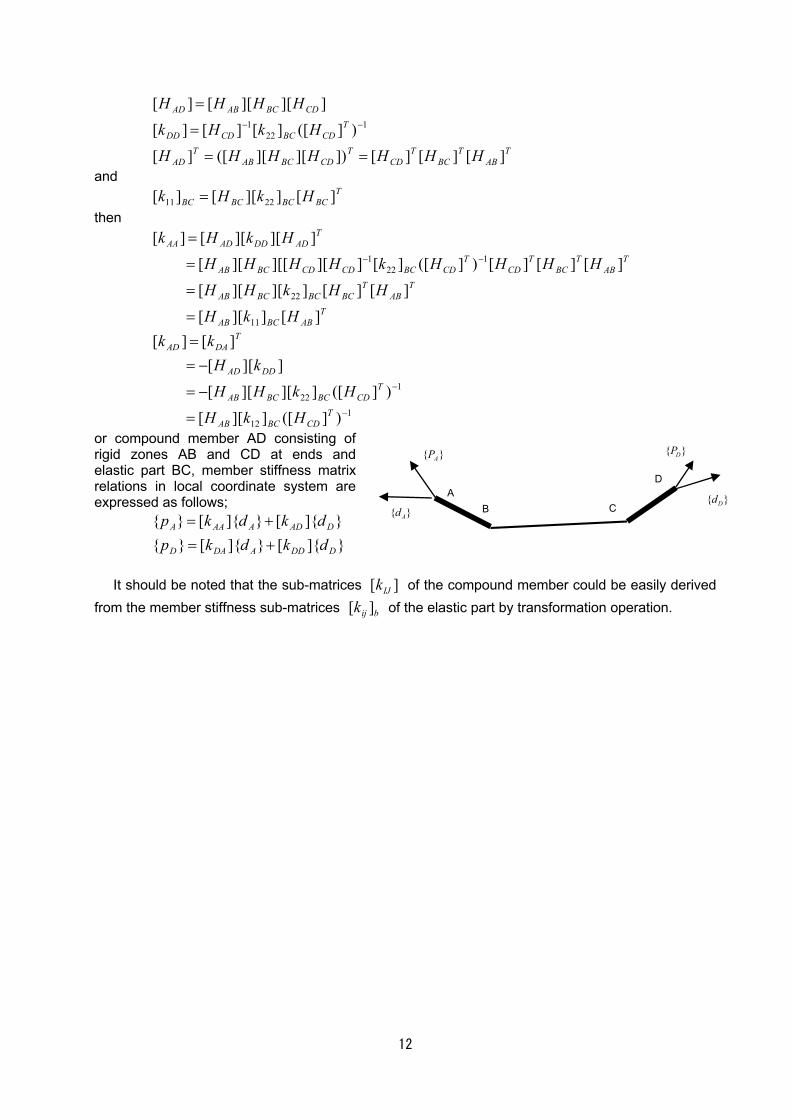
12

T

ABT

BCT

CDT

CDBCABT

AD

TCDBCCDDD

CDBCABAD

HHHHHHH

HkHk

HHHH

][][][])][][([][

)]([][][][

]][][[][1

221

==

=

=−−

and T

BCBCBCBC HkHk ][]][[][ 2211 = then

TABBCAB

TAB

TBCBCBCAB

TAB

TBC

TCD

TCDBCCDCDBCAB

TADDDADAA

HkH

HHkHH

HHHHkHHHHHkHk

][]][[

][][]][][[

][][][)]([][]][][[][[]][][[][

11

22

122

1

=

=

=

=−−

112

122

)]([]][[

)]([]][][[

]][[][][

−

−

=

−=

−==

TCDBCAB

TCDBCBCAB

DDAD

TDAAD

HkH

HkHH

kHkk

or compound member AD consisting of rigid zones AB and CD at ends and elastic part BC, member stiffness matrix relations in local coordinate system are expressed as follows;

}]{[}]{[}{}]{[}]{[}{

DDDADAD

DADAAAA

dkdkpdkdkp

+=+=

It should be noted that the sub-matrices [ ]IJk of the compound member could be easily derived

from the member stiffness sub-matrices [ ]kij b of the elastic part by transformation operation.

AB C

D

}{ AP { }DP

{ }Dd { }Ad

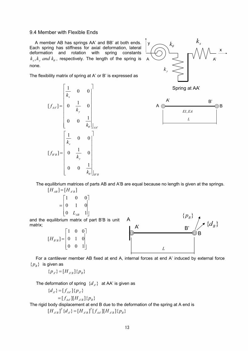
13

9.4 Member with Flexible Ends

A member AB has springs AA’ and BB’ at both ends. Each spring has stiffness for axial deformation, lateral deformation and rotation with spring constants

,x yk k and kθ , respectively. The length of the spring is none. The flexibility matrix of spring at A’ or B’ is expressed as

'

'

'

'

1 0 0

1[ ] 0 0

10 0

1 0 0

1[ ] 0 0

10 0

x

AAy

AA

x

B By

B B

k

fk

k

k

fk

k

θ

θ

=

=

The equilibrium matrices of parts AB and A’B are equal because no length is given at the springs.

'[ ] [ ]1 0 00 1 00 1

AB A B

AB

H H

L

=

=

and the equilibrium matrix of part B’B is unit matrix;

'

1 0 0[ ] 0 1 0

0 0 1B BH

=

For a cantilever member AB fixed at end A, internal forces at end A’ induced by external force

{ }Bp is given as ' '{ } [ ]{ }A A B Bp H p=

The deformation of spring '{ }Ad at AA’ is given as

' ' '

' '

{ } [ ]{ }[ ][ ]{ }

A AA A

AA A B B

d f pf H p

==

The rigid body displacement at end B due to the deformation of the spring at A end is ' ' ' ' '[ ] { } [ ] [ ][ ]{ }T T

A B A A B AA A B BH d H f H p=

kθ

yk

xk

xy

A A’

Spring at AA’

A BA’ B’

,EI EA

L

B

A’ B’

L

{ }Bp

{ }BdA

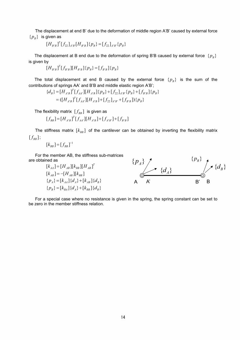
14

The displacement at end B’ due to the deformation of middle region A’B’ caused by external force { }Bp is given as

' 22 ' ' ' 22 ' '[ ] [ ] [ ]{ } [ ] { }TB B A B B B B A B BH f H p f p=

The displacement at B end due to the deformation of spring B’B caused by external force { }Bp

is given by ' ' ' '[ ] [ ][ ]{ } [ ]{ }T

B B B B B B B B B BH f H p f p=

The total displacement at end B caused by the external force { }Bp is the sum of the contributions of springs AA’ and B’B and middle elastic region A’B’;

' ' ' 22 ' ' '

' ' ' 22 ' ' '

{ } [ ] [ ][ ]{ } [ ] { } [ ]{ }([ ] [ ][ ] [ ] [ ]){ }

TB A B AA A B B A B B B B B

TA B AA A B A B B B B

d H f H p f p f p

H f H f f p

= + +

= + +

The flexibility matrix [ ]BBf is given as

' ' ' ' ' '[ ] [ ] [ ][ ] [ ] [ ]TBB A B AA A B A B B Bf H f H f f= + +

The stiffness matrix [ ]BBk of the cantilever can be obtained by inverting the flexibility matrix

[ ]BBf ;

1[ ] [ ]BB BBk f −= For the member AB, the stiffness sub-matrices

are obtained as

[ ] [ ][ ][ ][ ] [ ][ ]

TAA AB BB AB

AB AB BB

k H k Hk H k

== −

{ } [ ]{ } [ ]{ }{ } [ ]{ } [ ]{ }

A AA A AB B

B BA A BB B

p k d k dp k d k d

= += +

For a special case where no resistance is given in the spring, the spring constant can be set to

be zero in the member stiffness relation.

BA’ B’

{ }Bp{ }Bd

A

{ }Ad

{ }Ap

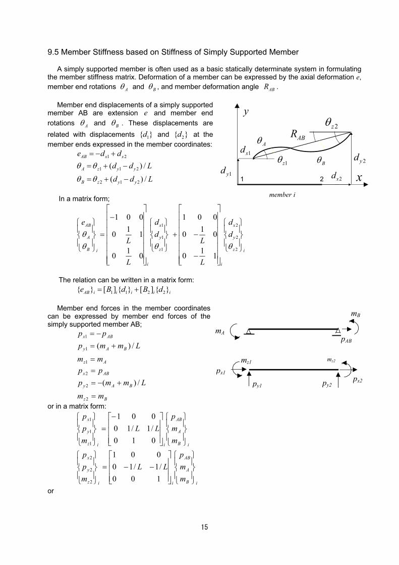
15

9.5 Member Stiffness based on Stiffness of Simply Supported Member

A simply supported member is often used as a basic statically determinate system in formulating the member stiffness matrix. Deformation of a member can be expressed by the axial deformation e, member end rotations Aθ and Bθ , and member deformation angle ABR .

Member end displacements of a simply supported member AB are extension e and member end rotations Aθ and Bθ . These displacements are related with displacements 1{ }d and 2{ }d at the member ends expressed in the member coordinates:

1 2

1 1 2

2 1 2

( ) /

( ) /

AB x x

A z y y

B z y y

e d dd d L

d d L

θ θ

θ θ

= − += + −

= + −

In a matrix form;

1 2

1 2

1 2

1 0 0 1 0 01 10 1 0 0

1 10 0 0 1

AB x x

A y y

B z zi i

i i

e d dd d

L L

L L

θθ θ θ

−

= + −

−

The relation can be written in a matrix form: 1 1 2 2{ } [ ] { } [ ] { }AB i i i i ie B d B d= + Member end forces in the member coordinates

can be expressed by member end forces of the simply supported member AB;

Az

BAy

ABx

mm

Lmmppp

=

+=−=

1

1

1

/)(

Bz

BAy

ABx

mm

Lmmppp

=

+−==

2

2

2

/)(

or in a matrix form:

iB

A

AB

iiz

y

x

iB

A

AB

iiz

y

x

mmp

LLmpp

mmp

LLmpp

−−=

−=

100/1/10

001

010/1/10001

2

2

2

1

1

1

or

mA

mB

pAB

px1px2py1 py2

mz1 mz2

1 2

2zθ

2xd

2yd

ABR

1zθ

1xd

1ydBθ

Aθ

y

xmember i

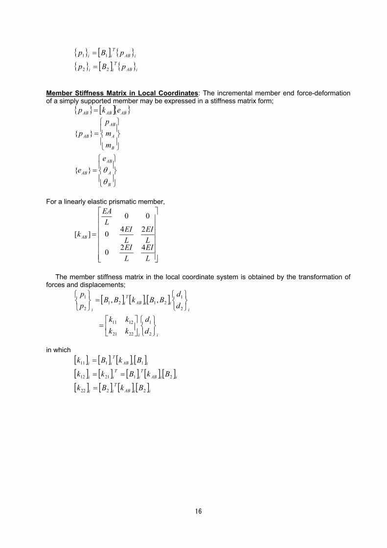
16

{ } [ ] { }{ } [ ] { }iAB

Tii

iABT

ii

pBp

pBp

22

11

=

=

Member Stiffness Matrix in Local Coordinates: The incremental member end force-deformation of a simply supported member may be expressed in a stiffness matrix form; { } [ ]{ }ABABAB ekp =

=

=

B

A

AB

AB

B

A

AB

AB

ee

mmp

p

θθ}{

}{

For a linearly elastic prismatic member,

=

LEI

LEI

LEI

LEI

LEA

k AB

420

240

00

][

The member stiffness matrix in the local coordinate system is obtained by the transformation of

forces and displacements;

[ ] [ ] [ ]

ii

iiiAB

Ti

i

dd

kkkk

dd

BBkBBpp

=

=

2

1

2221

1211

2

12121

2

1 ,,

in which

[ ] [ ] [ ] [ ][ ] [ ] [ ] [ ] [ ][ ] [ ] [ ] [ ]iiAB

Tii

iiABT

iT

ii

iiABT

ii

BkBk

BkBkk

BkBk

2222

212112

1111

=

==

=

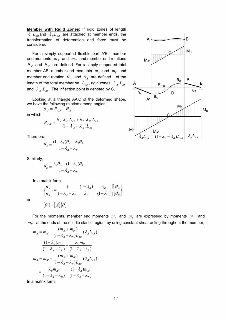
17

Member with Rigid Zones: If rigid zones of length λ A ABL and λ B ABL are attached at member ends, the transformation of deformation and force must be considered.

For a simply supported flexible part A'B', member

end moments mA' and mB' and member end rotations θ A' and θ B' are defined. For a simply supported total member AB, member end moments mA and mB and member end rotation θ A and θ B are defined. Let the length of the total member be LAB , rigid zones λ A ABL and λ B ABL . The inflection point is denoted by C.

Looking at a triangle AA'C of the deformed shape, we have the following relation among angles,

θ θA A B AR' ' '= + in which

R L LLA B

A A AB B B AB

A B AB' ' ( )=

+− −

θ λ θ λλ λ1

Therefore,

' (1 )1

B A B BA

A B

λ θ λ θθλ λ

− +=

− −

Similarly,

' (1 )1

A A A BB

A B

λ θ λ θθλ λ+ −

=− −

In a matrix form,

'

'

(1 )1(1 )1

B B AA

A A BA BB

λ λ θθλ λ θλ λθ−

= −− −

or { } [ ]{ }θθ A=' For the moments, member end moments Am and Bm are expressed by moments 'Am and

'Bm at the ends of the middle elastic region, by using constant shear acting throughout the member;

' ''

' '

' ''

' '

( ) ( )(1 )

(1 )(1 ) (1 )

( ) ( )(1 )

(1 )(1 ) (1 )

A BA A A AB

A B AB

B A A B

A B A B

A BB B B AB

A B AB

B A A B

A B A B

m mm m LL

m m

m mm m LL

m m

λλ λ

λ λλ λ λ λ

λλ λ

λ λλ λ λ λ

+= +

− −−

= +− − − −

+= +

− −−

= +− − − −

In a matrix form,

A' B'

MB’

MA’

A

A'

B'B

θAθB

θB’

θA’

RA’B’

MA

MB

MA’

MB’

C

C

D

A ABLλ (1 )A B ABLλ λ− − B ABLλ

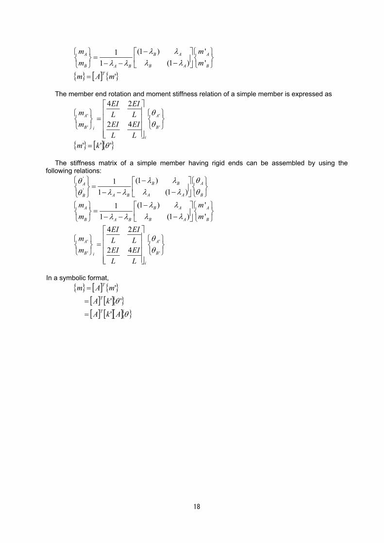
18

(1 ) '1

(1 ) '1A B A A

B B A BA B

m mm m

λ λλ λλ λ−

= −− −

{ } [ ] { }'mAm T= The member end rotation and moment stiffness relation of a simple member is expressed as

' '

' '

4 2

2 4A A

B Bi

i

EI EIm L Lm EI EI

L L

θθ

=

{ } [ ]{ }''' θkm = The stiffness matrix of a simple member having rigid ends can be assembled by using the

following relations:

'

'

(1 )1(1 )1

B B AA

A A BA BB

λ λ θθλ λ θλ λθ−

= −− −

(1 ) '1

(1 ) '1A B A A

B B A BA B

m mm m

λ λλ λλ λ−

= −− −

' '

' '

4 2

2 4A A

B Bi

i

EI EIm L Lm EI EI

L L

θθ

=

In a symbolic format,

{ } [ ] { }[ ] [ ]{ }[ ] [ ][ ]{ }θ

θ

AkA

kA

mAm

T

T

T

'

''

'

=

=

=

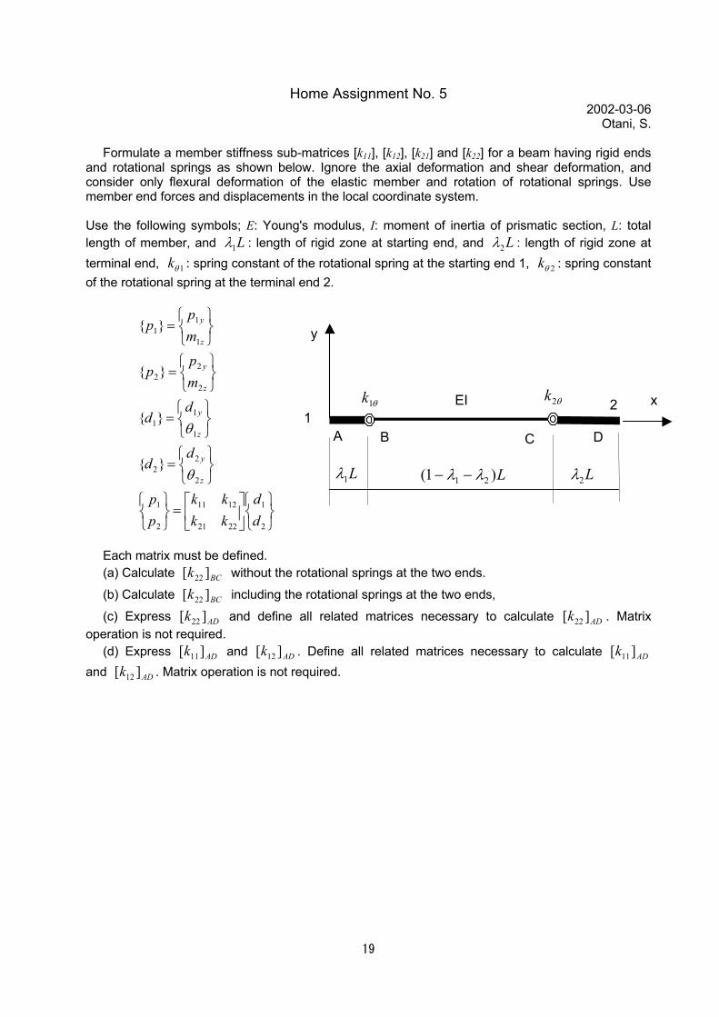
19

Home Assignment No. 5 2002-03-06

Otani, S. Formulate a member stiffness sub-matrices [k11], [k12], [k21] and [k22] for a beam having rigid ends

and rotational springs as shown below. Ignore the axial deformation and shear deformation, and consider only flexural deformation of the elastic member and rotation of rotational springs. Use member end forces and displacements in the local coordinate system.

Use the following symbols; E: Young's modulus, I: moment of inertia of prismatic section, L: total length of member, and L1λ : length of rigid zone at starting end, and L2λ : length of rigid zone at terminal end, 1θk : spring constant of the rotational spring at the starting end 1, 2θk : spring constant of the rotational spring at the terminal end 2.

=

=

=

=

=

2

1

2221

1211

2

1

2

22

1

11

2

22

1

11

}{

}{

}{

}{

dd

kkkk

pp

dd

dd

mp

p

mp

p

z

y

z

y

z

y

z

y

θ

θ

Each matrix must be defined. (a) Calculate BCk ][ 22 without the rotational springs at the two ends.

(b) Calculate BCk ][ 22 including the rotational springs at the two ends,

(c) Express ADk ][ 22 and define all related matrices necessary to calculate ADk ][ 22 . Matrix operation is not required.

(d) Express ADk ][ 11 and ADk ][ 12 . Define all related matrices necessary to calculate ADk ][ 11 and ADk ][ 12 . Matrix operation is not required.

1

y

x2θ1k θ2kEI

L1λ L2λL)1( 21 λλ −−

A B C D

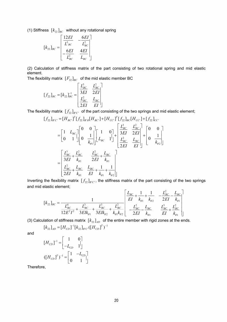
20

(1) Stiffness 22[ ]BCk without any rotational spring

3 2

22

2

12 6

[ ]6 4

BC BCBC

BC BC

EI EIL L

kEI EI

L L

− = −

(2) Calculation of stiffness matrix of the part consisting of two rotational spring and mid elastic element. The flexibility matrix 22[ ]BCF of the mid elastic member BC

3 2

122 22 2

3 2[ ] [ ]

2

BC BC

BC BCBC BC

L LEI EIf k

L LEI EI

−

= =

The flexibility matrix 22 ' '[ ]B Cf of the part consisting of the two springs and mid elastic element;

22 ' ' ' 22 ' ' ' 22 ' 22 '

3 2

2

1 2

3 2 2

1 1

2

[ ] [ ] [ ] [ ] [ ] [ ] [ ] [ ]

0 0 0 01 01 3 21 10 010 1

2

3 2

2

T TB C BC B B BC CC BC CC CC

BC BC

BC

BC BC BC

BC BC BC BC

BC B

f H f H H f H f

L LL EI EI

L L Lk kEI EI

L L L LEI k EI k

L LEI

θ θ

θ θ

= + +

= + +

+ +

=+

1 1 2

1 1C BCLk EI k kθ θ θ

+ +

Inverting the flexibility matrix 22 ' '[ ]B Cf , the stiffness matrix of the part consisting of the two springs and mid elastic element;

2

1 2 122 4 3 3 2 2 3 2

2 21 2 1 2 1 1

1 121[ ]

12 3 3 2

BC BC BC

BCBC BC BC BC BC BC BC BC

L L LEI k k EI k

kL L L L L L L LE I EIk EIk k k EI k EI k

θ θ θ

θ θ θ θ θ θ

+ + − −

=

+ + + − − +

(3) Calculation of stiffness matrix 22[ ]ADk of the entire member with rigid zones at the ends.

1 122 22 ' '[ ] [ ] [ ] ([ ] )T

AD CD B C CDk H k H− −= and

1

1

1 0[ ]

1

1([ ] )

0 1

CDCD

CDTCD

HL

LH

−

−

= −

− =

Therefore,

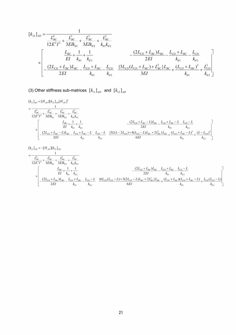
21

22 4 3 3 2

2 21 2 1 2

1 2 1 2

2 2 2

1 2 1 2

1[ ]

12 3 3(2 )1 1

2

(2 ) {3 ( ) } ( )2 3

ADBC BC BC BC

BC CD BC BC CD BC CD

CD BC BC CD BC CD CD CD BC BC BC CD BC CD

kL L L LE I EIk EIk k k

L L L L L L LEI k k EI k k

L L L L L L L L L L L L L LEI k k EI k k

θ θ θ θ

θ θ θ θ

θ θ θ θ

=+ + +

+ + + + − − − × + + + + +− − − + +

(3) Other stiffness sub-matrices 11[ ]ADk and 12[ ]ADk

11 22

4 3 3 2

2 21 2 1 2

1 2 1 22

1 2

[ ] [ ][ ] [ ]1

12 3 3(2 )1 1

2

(2 ) {3 ( 2 ) 6( ) 2 }2

TAD AD AD AD

BC BC BC BC

BC CD BC BC CD BC CD

CD BC BC CD BC CD CD CD BC BC

k H k H

L L L LE I EIk EIk k k

L L L L L L L L L LEI k k EI k k

L L L L L L L L L L L L L L L L LEI k k

θ θ θ θ

θ θ θ θ

θ θ

=

=+ + +

+ − + − −+ + − − −

×+ − + − − − + − +

− − −2 2

1 2

( ) ( )6

BC CD BC CDL L L L LEI k kθ θ

+ − −

+ +

12 22

4 3 3 2

2 21 2 1 2

1 2 1 22

1 2

[ ] [ ][ ]1

12 3 3(2 )1 1

2

(2 ) {6 ( ) 3(2 ) 2 } (2 6

AD AD AD

BC BC BC BC

BC CD BC BC CD BC CD

CD BC BC CD BC CD CD CD CD BC BC BC CD

k H k

L L L LE I EIk EIk k k

L L L L L L L LEI k k EI k k

L L L L L L L L L L L L L L L LEI k k EI

θ θ θ θ

θ θ θ θ

θ θ

= −

=+ + +

+ + −+ + − − −

×+ + − − + − + +

− − − +1 2

)( ) ( )BC CD BC CD CDL L L L L L Lk kθ θ

+ − −

+

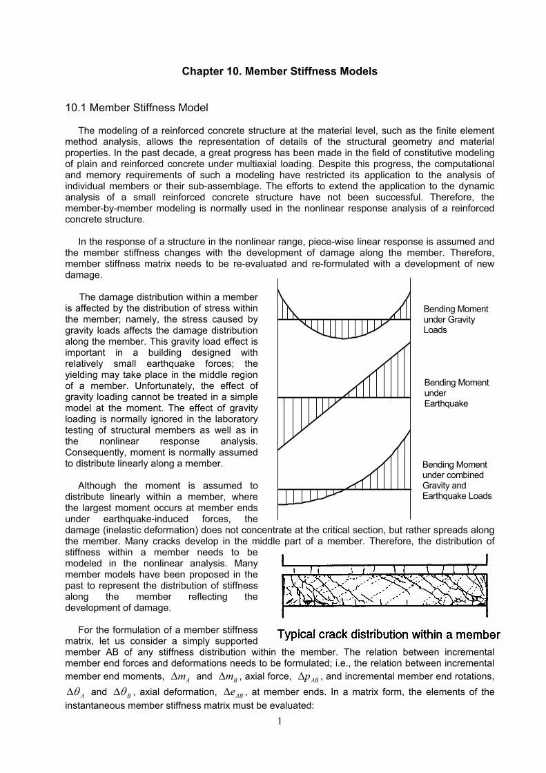
1

Chapter 10. Member Stiffness Models

10.1 Member Stiffness Model

The modeling of a reinforced concrete structure at the material level, such as the finite element

method analysis, allows the representation of details of the structural geometry and material properties. In the past decade, a great progress has been made in the field of constitutive modeling of plain and reinforced concrete under multiaxial loading. Despite this progress, the computational and memory requirements of such a modeling have restricted its application to the analysis of individual members or their sub-assemblage. The efforts to extend the application to the dynamic analysis of a small reinforced concrete structure have not been successful. Therefore, the member-by-member modeling is normally used in the nonlinear response analysis of a reinforced concrete structure.

In the response of a structure in the nonlinear range, piece-wise linear response is assumed and

the member stiffness changes with the development of damage along the member. Therefore, member stiffness matrix needs to be re-evaluated and re-formulated with a development of new damage.

The damage distribution within a member

is affected by the distribution of stress within the member; namely, the stress caused by gravity loads affects the damage distribution along the member. This gravity load effect is important in a building designed with relatively small earthquake forces; the yielding may take place in the middle region of a member. Unfortunately, the effect of gravity loading cannot be treated in a simple model at the moment. The effect of gravity loading is normally ignored in the laboratory testing of structural members as well as in the nonlinear response analysis. Consequently, moment is normally assumed to distribute linearly along a member.

Although the moment is assumed to

distribute linearly within a member, where the largest moment occurs at member ends under earthquake-induced forces, the damage (inelastic deformation) does not concentrate at the critical section, but rather spreads along the member. Many cracks develop in the middle part of a member. Therefore, the distribution of stiffness within a member needs to be modeled in the nonlinear analysis. Many member models have been proposed in the past to represent the distribution of stiffness along the member reflecting the development of damage.

For the formulation of a member stiffness

matrix, let us consider a simply supported member AB of any stiffness distribution within the member. The relation between incremental member end forces and deformations needs to be formulated; i.e., the relation between incremental member end moments, Am∆ and Bm∆ , axial force, ABp∆ , and incremental member end rotations,

Aθ∆ and Bθ∆ , axial deformation, ABe∆ , at member ends. In a matrix form, the elements of the instantaneous member stiffness matrix must be evaluated:

Bending Moment under Gravity Loads

Bending Moment under Earthquake

Bending Moment under combined Gravity and Earthquake Loads

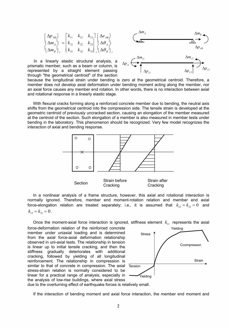
2

iB

A

AB

iiB

A

AB e

kkkkkkkkk

mmp

∆∆∆

=

∆∆∆

θθ

333231

232221

131211

In a linearly elastic structural analysis, a

prismatic member, such as a beam or column, is represented by a straight element passing through "the geometrical centroid" of the section because the longitudinal strain under bending is zero at the geometrical centroid. Therefore, a member does not develop axial deformation under bending moment acting along the member, nor an axial force causes any member end rotation. In other words, there is no interaction between axial and rotational response in a linearly elastic stage.

With flexural cracks forming along a reinforced concrete member due to bending, the neutral axis

shifts from the geometrical centroid into the compression side. The tensile strain is developed at the geometric centroid of previously uncracked section, causing an elongation of the member measured at the centroid of the section. Such elongation of a member is also measured in member tests under bending in the laboratory. This phenomenon should be recognized. Very few model recognizes the interaction of axial and bending response.

Strain beforeCracking

Strain afterCrackingSection

In a nonlinear analysis of a frame structure, however, this axial and rotational interaction is

normally ignored. Therefore, member end moment-rotation relation and member end axial force-elongation relation are treated separately; i.e., it is assumed that k k12 21 0= = and k k13 31 0= = .

Once the moment-axial force interaction is ignored, stiffness element k11 represents the axial

force-deformation relation of the reinforced concrete member under uniaxial loading and is determined from the axial force-axial deformation relationship observed in uni-axial tests. The relationship in tension is linear up to initial tensile cracking, and then the stiffness gradually deteriorates with additional cracking, followed by yielding of all longitudinal reinforcement. The relationship in compression is similar to that of concrete in compression. The axial stress-strain relation is normally considered to be linear for a practical range of analysis, especially in the analysis of low-rise buildings, where axial stress due to the overturning effect of earthquake forces is relatively small.

If the interaction of bending moment and axial force interaction, the member end moment and

Am∆Bm∆

ABp∆

1xp∆2xp∆

1yp∆ 2yp∆

1zm∆ 2zm∆

Yielding

Strain

Stress

Ccompresson

Tension

Yielding

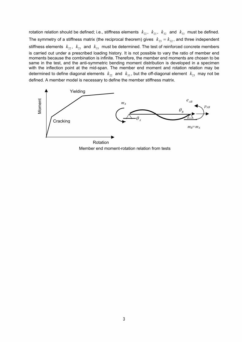
3

rotation relation should be defined; i.e., stiffness elements 22k , 23k , 32k and 33k must be defined.

The symmetry of a stiffness matrix (the reciprocal theorem) gives 3223 kk = , and three independent

stiffness elements 22k , 23k and 33k must be determined. The test of reinforced concrete members is carried out under a prescribed loading history. It is not possible to vary the ratio of member end moments because the combination is infinite. Therefore, the member end moments are chosen to be same in the test, and the anti-symmetric bending moment distribution is developed in a specimen with the inflection point at the mid-span. The member end moment and rotation relation may be determined to define diagonal elements 22k and 33k , but the off-diagonal element 23k may not be defined. A member model is necessary to define the member stiffness matrix.

Rotation

Mom

ent

Cracking

Yielding

mA

mB=mA Aθ

Bθ

ABepAB

Member end moment-rotation relation from tests

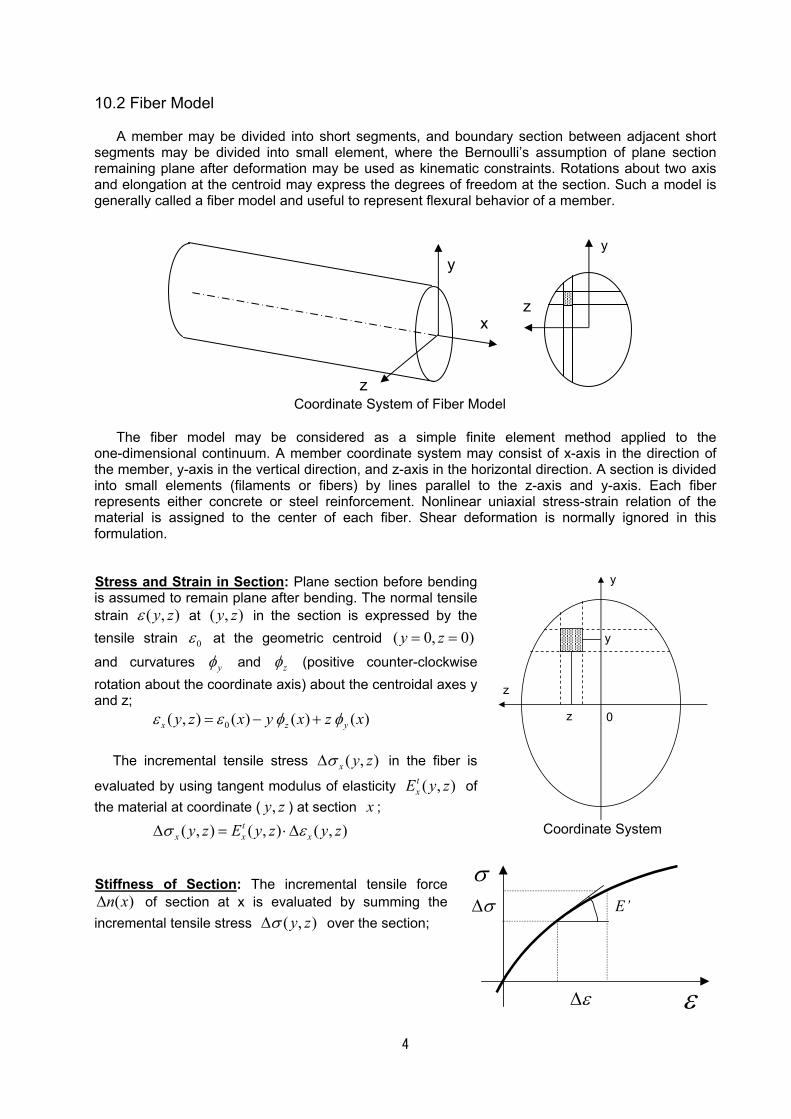
4

10.2 Fiber Model

A member may be divided into short segments, and boundary section between adjacent short segments may be divided into small element, where the Bernoulli’s assumption of plane section remaining plane after deformation may be used as kinematic constraints. Rotations about two axis and elongation at the centroid may express the degrees of freedom at the section. Such a model is generally called a fiber model and useful to represent flexural behavior of a member.

The fiber model may be considered as a simple finite element method applied to the

one-dimensional continuum. A member coordinate system may consist of x-axis in the direction of the member, y-axis in the vertical direction, and z-axis in the horizontal direction. A section is divided into small elements (filaments or fibers) by lines parallel to the z-axis and y-axis. Each fiber represents either concrete or steel reinforcement. Nonlinear uniaxial stress-strain relation of the material is assigned to the center of each fiber. Shear deformation is normally ignored in this formulation.

Stress and Strain in Section: Plane section before bending is assumed to remain plane after bending. The normal tensile strain ( , )y zε at ( , )y z in the section is expressed by the tensile strain 0ε at the geometric centroid ( 0, 0)y z= =

and curvatures yφ and zφ (positive counter-clockwise rotation about the coordinate axis) about the centroidal axes y and z; 0( , ) ( ) ( ) ( )x z yy z x y x z xε ε φ φ= − +

The incremental tensile stress ( , )x y zσ∆ in the fiber is

evaluated by using tangent modulus of elasticity ( , )txE y z of

the material at coordinate ( ,y z ) at section x ;

( , ) ( , ) ( , )tx x xy z E y z y zσ ε∆ = ⋅∆

Stiffness of Section: The incremental tensile force

( )n x∆ of section at x is evaluated by summing the incremental tensile stress ( , )y zσ∆ over the section;

x

y

z

y

z

Coordinate System of Fiber Model

y

z

y

z

0

Coordinate System

σ

ε

E’

ε∆

σ∆

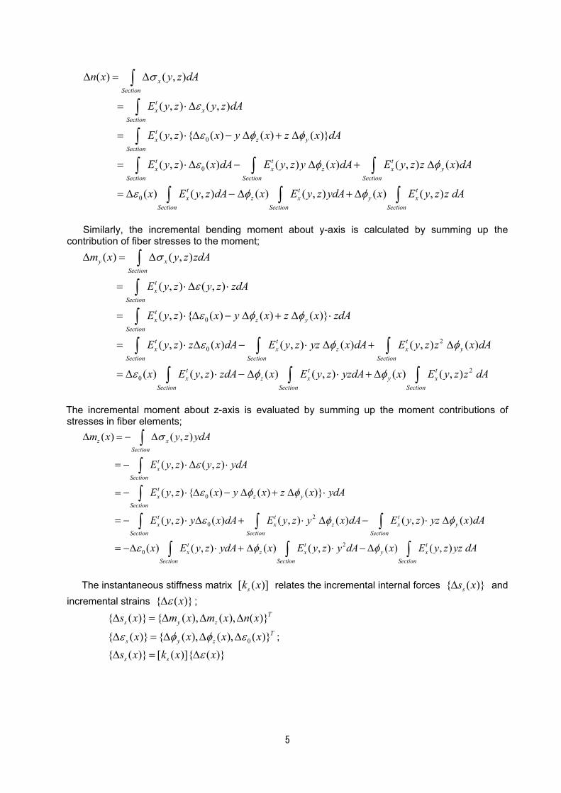
5

0

0

0

( ) ( , )

( , ) ( , )

( , ) { ( ) ( ) ( )}

( , ) ( ) ( , ) ( ) ( , ) ( )

( ) ( , )

xSection

tx x

Section

tx z y

Section

t t tx x z x y

Section Section Section

tx

Section

n x y z dA

E y z y z dA

E y z x y x z x dA

E y z x dA E y z y x dA E y z z x dA

x E y z dA

σ

ε

ε φ φ

ε φ φ

ε

∆ = ∆

= ⋅∆

= ⋅ ∆ − ∆ + ∆

= ⋅∆ − ∆ + ∆

= ∆ −

∫

∫

∫

∫ ∫ ∫

∫ ( ) ( , ) ( ) ( , )t tz x y x

Section Section

x E y z ydA x E y z z dAφ φ∆ + ∆∫ ∫

Similarly, the incremental bending moment about y-axis is calculated by summing up the

contribution of fiber stresses to the moment;

0

20

0

( ) ( , )

( , ) ( , )

( , ) { ( ) ( ) ( )}

( , ) ( ) ( , ) ( ) ( , ) ( )

( ) ( , )

y xSection

tx

Section

tx z y

Section

t t tx x z x y

Section Section Section

tx

m x y z zdA

E y z y z zdA

E y z x y x z x zdA

E y z z x dA E y z yz x dA E y z z x dA

x E y z z

σ

ε

ε φ φ

ε φ φ

ε

∆ = ∆

= ⋅∆ ⋅

= ⋅ ∆ − ∆ + ∆ ⋅

= ⋅ ∆ − ⋅ ∆ + ∆

= ∆ ⋅

∫

∫

∫

∫ ∫ ∫2( ) ( , ) ( ) ( , )t t

z x y xSection Section Section

dA x E y z yzdA x E y z z dAφ φ− ∆ ⋅ + ∆∫ ∫ ∫

The incremental moment about z-axis is evaluated by summing up the moment contributions of stresses in fiber elements;

0

20

0

( ) ( , )

( , ) ( , )

( , ) { ( ) ( ) ( )}

( , ) ( ) ( , ) ( ) ( , ) ( )

( ) (

z xSection

tx

Section

tx z y

Section

t t tx x z x y

Section Section Section

tx

m x y z ydA

E y z y z ydA

E y z x y x z x ydA

E y z y x dA E y z y x dA E y z yz x dA

x E

σ

ε

ε φ φ

ε φ φ

ε

∆ = − ∆

= − ⋅∆ ⋅

= − ⋅ ∆ − ∆ + ∆ ⋅

= − ⋅ ∆ + ⋅ ∆ − ⋅ ∆

= −∆

∫

∫

∫

∫ ∫ ∫2, ) ( ) ( , ) ( ) ( , )t t

z x y xSection Section Section

y z ydA x E y z y dA x E y z yz dAφ φ⋅ + ∆ ⋅ − ∆∫ ∫ ∫

The instantaneous stiffness matrix [ ( )]sk x relates the incremental internal forces { ( )}ss x∆ and

incremental strains { ( )}xε∆ ;

{ ( )} { ( ), ( ), ( )}Ts y zs x m x m x n x∆ = ∆ ∆ ∆

0{ ( )} { ( ), ( ), ( )}Ts y zx x x xε φ φ ε∆ = ∆ ∆ ∆ ;

{ ( )} [ ( )]{ ( )}s ss x k x xε∆ = ∆

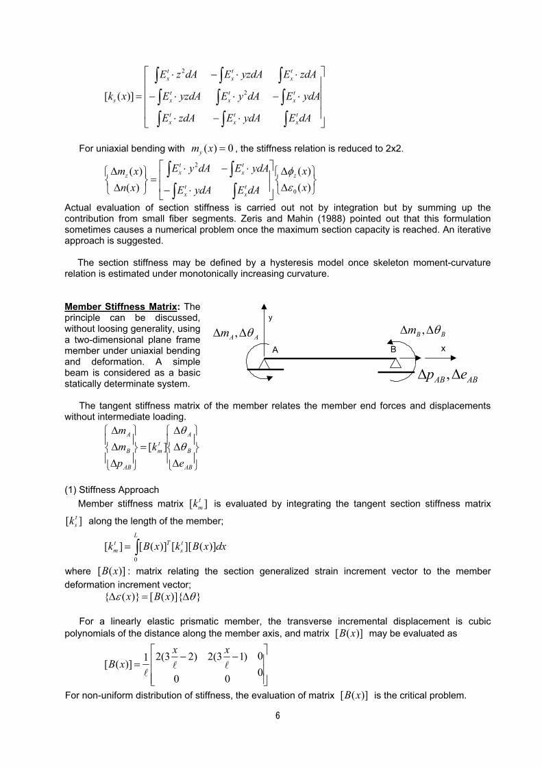
6

2

2[ ( )]

t t tx x x

t t ts x x x

t t tx x x

E z dA E yzdA E zdA

k x E yzdA E y dA E ydA

E zdA E ydA E dA

⋅ − ⋅ ⋅ = − ⋅ ⋅ − ⋅ ⋅ − ⋅

∫ ∫ ∫∫ ∫ ∫∫ ∫ ∫

For uniaxial bending with ( ) 0ym x = , the stiffness relation is reduced to 2x2.

2

0

( )( )( )( )

t tx x zz

t tx x

E y dA E ydA xm xxn x E ydA E dA

φε

⋅ − ⋅ ∆∆ = ∆ ∆ − ⋅

∫ ∫∫ ∫

Actual evaluation of section stiffness is carried out not by integration but by summing up the contribution from small fiber segments. Zeris and Mahin (1988) pointed out that this formulation sometimes causes a numerical problem once the maximum section capacity is reached. An iterative approach is suggested.

The section stiffness may be defined by a hysteresis model once skeleton moment-curvature relation is estimated under monotonically increasing curvature. Member Stiffness Matrix: The principle can be discussed, without loosing generality, using a two-dimensional plane frame member under uniaxial bending and deformation. A simple beam is considered as a basic statically determinate system.

The tangent stiffness matrix of the member relates the member end forces and displacements without intermediate loading.

∆∆∆

=

∆∆∆

AB

B

Atm

AB

B

A

ek

pmm

θθ

][

(1) Stiffness Approach

Member stiffness matrix [ ]tmk is evaluated by integrating the tangent section stiffness matrix

[ ]tsk along the length of the member;

0

[ ] [ ( )] [ ][ ( )]L

t T tm sk B x k B x dx= ∫

where [ ( )]B x : matrix relating the section generalized strain increment vector to the member deformation increment vector; { ( )} [ ( )]{ }x B xε θ∆ = ∆

For a linearly elastic prismatic member, the transverse incremental displacement is cubic polynomials of the distance along the member axis, and matrix [ ( )]B x may be evaluated as

02(3 2) 2(3 1)1[ ( )]00 0

x xB x

− − =

l ll

For non-uniform distribution of stiffness, the evaluation of matrix [ ( )]B x is the critical problem.

A B

,A Am θ∆ ∆ ,B Bm θ∆ ∆

x

y

ABAB ep ∆∆ ,

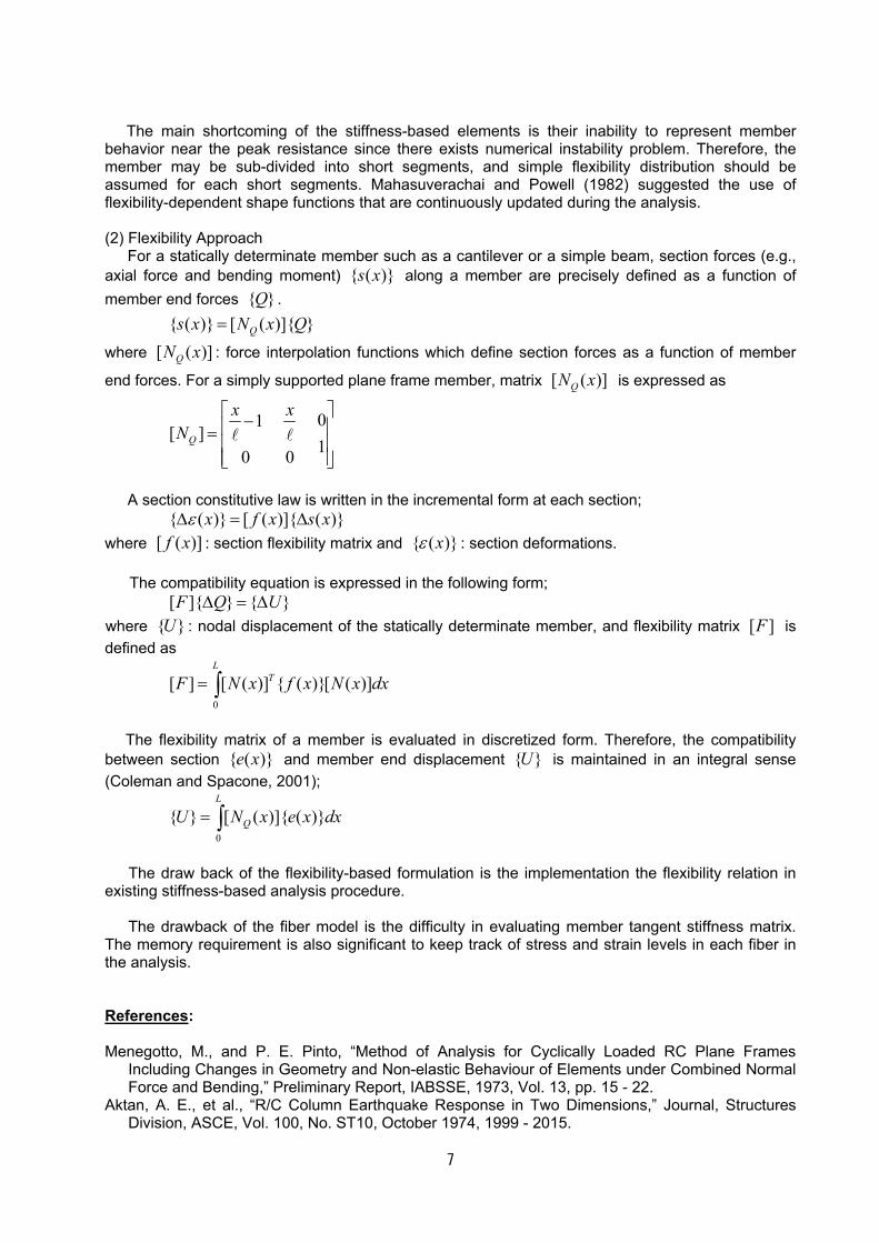
7

The main shortcoming of the stiffness-based elements is their inability to represent member

behavior near the peak resistance since there exists numerical instability problem. Therefore, the member may be sub-divided into short segments, and simple flexibility distribution should be assumed for each short segments. Mahasuverachai and Powell (1982) suggested the use of flexibility-dependent shape functions that are continuously updated during the analysis. (2) Flexibility Approach

For a statically determinate member such as a cantilever or a simple beam, section forces (e.g., axial force and bending moment) { ( )}s x along a member are precisely defined as a function of member end forces { }Q . { ( )} [ ( )]{ }Qs x N x Q=

where [ ( )]QN x : force interpolation functions which define section forces as a function of member

end forces. For a simply supported plane frame member, matrix [ ( )]QN x is expressed as

01

[ ]10 0

Q

x xN

− = l l

A section constitutive law is written in the incremental form at each section;

{ ( )} [ ( )]{ ( )}x f x s xε∆ = ∆ where [ ( )]f x : section flexibility matrix and { ( )}xε : section deformations.

The compatibility equation is expressed in the following form; [ ]{ } { }F Q U∆ = ∆ where { }U : nodal displacement of the statically determinate member, and flexibility matrix [ ]F is defined as

0

[ ] [ ( )] { ( )}[ ( )]L

TF N x f x N x dx= ∫

The flexibility matrix of a member is evaluated in discretized form. Therefore, the compatibility

between section { ( )}e x and member end displacement { }U is maintained in an integral sense (Coleman and Spacone, 2001);

0

{ } [ ( )]{ ( )}L

QU N x e x dx= ∫

The draw back of the flexibility-based formulation is the implementation the flexibility relation in

existing stiffness-based analysis procedure.

The drawback of the fiber model is the difficulty in evaluating member tangent stiffness matrix. The memory requirement is also significant to keep track of stress and strain levels in each fiber in the analysis. References: Menegotto, M., and P. E. Pinto, “Method of Analysis for Cyclically Loaded RC Plane Frames

Including Changes in Geometry and Non-elastic Behaviour of Elements under Combined Normal Force and Bending,” Preliminary Report, IABSSE, 1973, Vol. 13, pp. 15 - 22.

Aktan, A. E., et al., “R/C Column Earthquake Response in Two Dimensions,” Journal, Structures Division, ASCE, Vol. 100, No. ST10, October 1974, 1999 - 2015.

8

Aziz, T. S., “Inelastic Dynamic Analysis of Building Frames,” Research Report R76-37, Department of Civil Engineering, Massachusetts Institute of Technology, Cambridge, MA, 1976.

Coleman, J., and E. Spacone, “Localization Issues in Force-based Frame Elements,” Journal, Structural Engineering, ASCE, Vol. 127, No. 11, November 2001, pp. 1257 - 1265.

Kaba, S. and S. A. Mahin, “Refined Modeling of Reinforced Concrete Columns for Seismic Analysis,” EERC Report 84/03, Earthquake Engineering Research Center, University of California, Berkeley, 1984.

Mahasuverachai, M., and G. H. Powell, “Inelastic Analysis of Piping and Tubular Structures,” EERC Report 82-27, Earthquake Engineering Research Center, University of California, Berkeley, 1982.

Mark, K., “Nonlinear Dynamic Response of Reinforced Concrete Frames,” Research Report R76-38, Department of Civil Engineering, Massachusetts Institute of Technology, Cambridge, MA, 1976.

Spacone, E., F. C. Filippou and F. F Taucer, “Fiber Beam-column Model for Non-linear Analysis of R/C Frames: Part I. Formulation,” Earthquake Engineering and Structural Dynamics, Vol. 25, 1996, pp. 711 - 725.

Spacone, E., F. C. Filippou and F. F Taucer, “Fiber Beam-column Model for Non-linear Analysis of R/C Frames: Part II. Applications,” Earthquake Engineering and Structural Dynamics, Vol. 25, 1996, pp. 727 - 742.

Zeris, C. and S. A. Mahin, “Analysis of Reinforced Concrete Beam-columns under uniaxial excitation, Journal, Structures Division, ASCE, Vol. 114, No. ST4, April 1988, pp. 804 - 820.

Zeris, C., and S. A. Mahin, “Behavior of Reinforced Concrete Structures subjected to Biaxial Excitation,” Journal, Structures Division, ASCE, Vol. 117, No. ST9, September 1991, pp. 2657 - 2673.

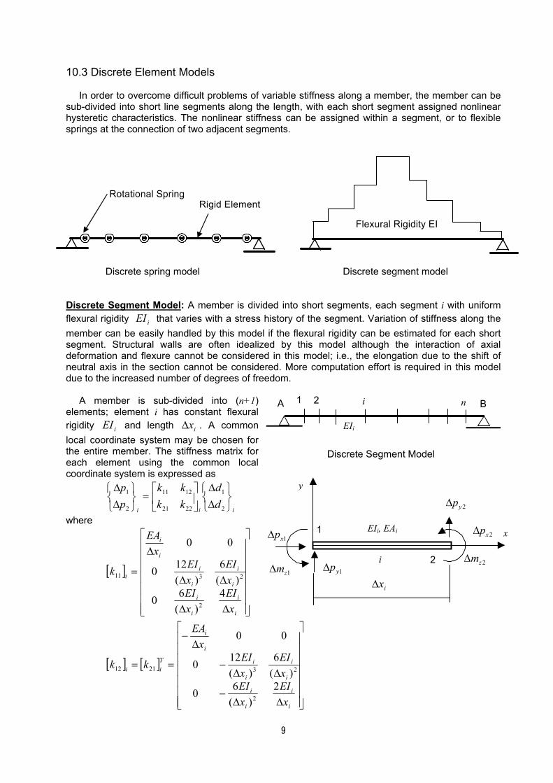
9

10.3 Discrete Element Models

In order to overcome difficult problems of variable stiffness along a member, the member can be sub-divided into short line segments along the length, with each short segment assigned nonlinear hysteretic characteristics. The nonlinear stiffness can be assigned within a segment, or to flexible springs at the connection of two adjacent segments.

Discrete spring model Discrete segment model Discrete Segment Model: A member is divided into short segments, each segment i with uniform flexural rigidity iEI that varies with a stress history of the segment. Variation of stiffness along the member can be easily handled by this model if the flexural rigidity can be estimated for each short segment. Structural walls are often idealized by this model although the interaction of axial deformation and flexure cannot be considered in this model; i.e., the elongation due to the shift of neutral axis in the section cannot be considered. More computation effort is required in this model due to the increased number of degrees of freedom.

A member is sub-divided into (n+1) elements; element i has constant flexural rigidity iEI and length ix∆ . A common local coordinate system may be chosen for the entire member. The stiffness matrix for each element using the common local coordinate system is expressed as

iii d

dkkkk

pp

∆∆

=

∆∆

2

1

2221

1211

2

1

where

[ ]

∆∆

∆∆

∆

=

i

i

i

i

i

i

i

i

i

i

i

xEI

xEI

xEI

xEI

xEA

k

4)(

60

)(6

)(120

00

2

2311

[ ] [ ]

∆∆−

∆∆−

∆−

==

i

i

i

i

i

i

i

i

i

i

Tii

xEI

xEI

xEI

xEI

xEA

kk

2)(

60

)(6

)(120

00

2

232112

A B 1 2 i n

EIi

Discrete Segment Model

Flexural Rigidity EI

Rotational Spring Rigid Element

x

y

1

2 i 2zm∆

2yp∆

2xp∆EIi, EAi 1xp∆

1yp∆1zm∆ix∆

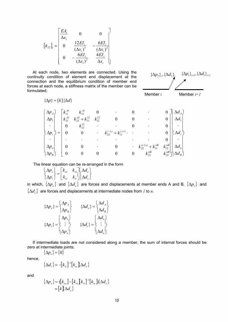
10

[ ]

∆∆−

∆−

∆

∆

=

i

i

i

i

i

i

i

i

i

i

i

xEI

xEI

xEI

xEI

xEA

k

4)(

60

)(6

)(120

00

2

2322

At each node, two elements are connected. Using the

continuity condition of element end displacement at the connection and the equilibrium condition of member end forces at each node, a stiffness matrix of the member can be formulated; }]{[}{ dkp ∆=∆

∆∆⋅

∆⋅

∆∆

+⋅⋅⋅⋅⋅⋅⋅⋅⋅⋅⋅+⋅⋅⋅⋅⋅+⋅⋅

=

∆∆⋅

∆⋅

∆∆

−

+−

B

n

i

A

nBnB

nBnBnn

iiii

AA

AA

B

n

i

A

dd

d

dd

kkkkk

kkk

kkkkkk

pp

p

pp

1

2221

1211,1

22

1,11

,122

1221

1212

1211

122

121

112

111

1

00000000

0000000000000

The linear equation can be re-arranged in the form

∆∆

=

∆∆

i

e

iiie

eiee

i

e

dd

kkkk

pp

in which, { }ep∆ and { }ed∆ are forces and displacements at member ends A and B, { }ip∆ and

{ }id∆ are forces and displacements at intermediate nodes from 1 to n.

∆

∆=∆

∆

∆=∆

∆∆

=∆

∆∆

=∆

n

i

n

i

B

Ae

B

Ae

d

dd

p

pp

dd

dpp

p

MM11

}{}{

}{}{

If intermediate loads are not considered along a member, the sum of internal forces should be

zero at intermediate joints; { } { }0=∆ ip hence, { } [ ] [ ]{ }eieiii dkkd ∆−=∆ −1 and

{ } [ ] [ ][ ] [ ] { }

[ ]{ }e

eieiieieee

dkdkkkkp

∆=∆−=∆ − )( 1

2 2{ } ,{ }i ip d∆ ∆

Member i Member i+1

1 1 1 1{ } ,{ }i ip d+ +∆ ∆

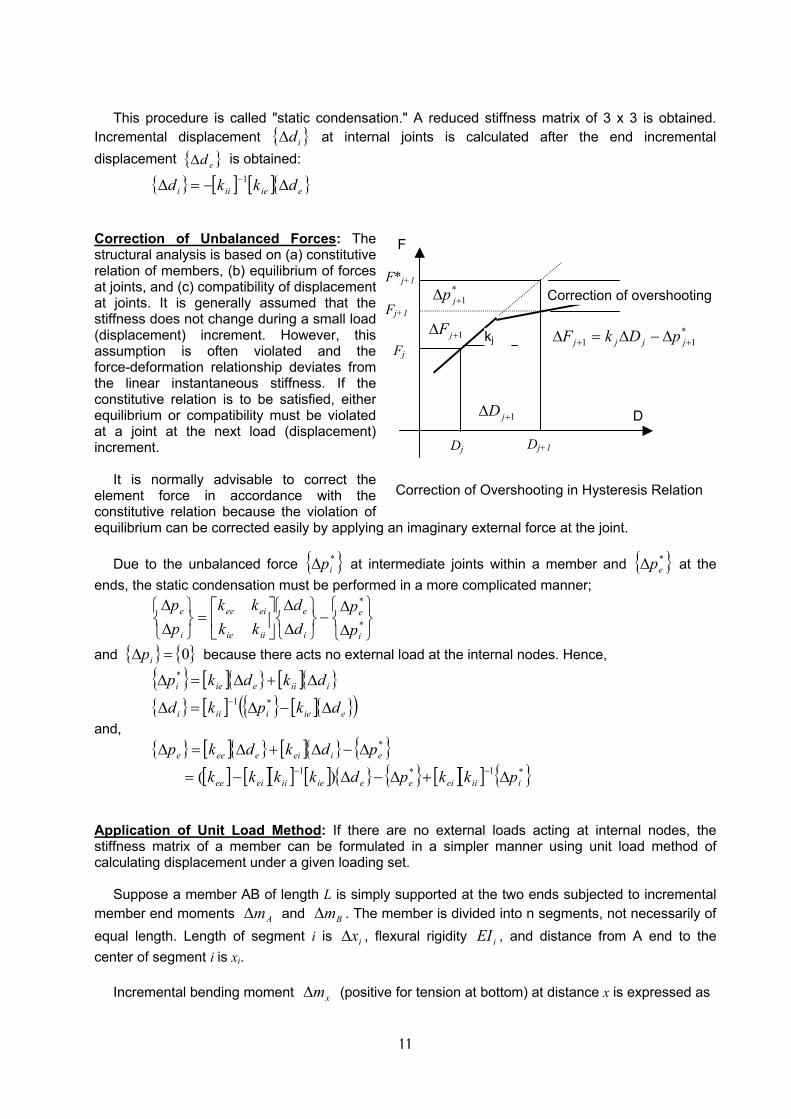
11

This procedure is called "static condensation." A reduced stiffness matrix of 3 x 3 is obtained.

Incremental displacement { }id∆ at internal joints is calculated after the end incremental displacement { }ed∆ is obtained:

{ } [ ] [ ]{ }eieiii dkkd ∆−=∆ −1 Correction of Unbalanced Forces: The structural analysis is based on (a) constitutive relation of members, (b) equilibrium of forces at joints, and (c) compatibility of displacement at joints. It is generally assumed that the stiffness does not change during a small load (displacement) increment. However, this assumption is often violated and the force-deformation relationship deviates from the linear instantaneous stiffness. If the constitutive relation is to be satisfied, either equilibrium or compatibility must be violated at a joint at the next load (displacement) increment.

It is normally advisable to correct the element force in accordance with the constitutive relation because the violation of equilibrium can be corrected easily by applying an imaginary external force at the joint.

Due to the unbalanced force { }*ip∆ at intermediate joints within a member and { }*

ep∆ at the ends, the static condensation must be performed in a more complicated manner;

∆∆

−

∆∆

=

∆∆

*

*

i

e

i

e

iiie

eiee

i

e

pp

dd

kkkk

pp

and { } { }0=∆ ip because there acts no external load at the internal nodes. Hence,

{ } [ ]{ } [ ]{ }{ } [ ] { } [ ]{ }( )eieiiii

iiieiei

dkpkd

dkdkp

∆−∆=∆

∆+∆=∆− *1

*

and,

{ } [ ]{ } [ ]{ } { }

[ ] [ ][ ] [ ] { } { } [ ][ ] { }*1*1

*

)( iiieieeieiieiee

eieieeee

pkkpdkkkk

pdkdkp

∆+∆−∆−=

∆−∆+∆=∆−−

Application of Unit Load Method: If there are no external loads acting at internal nodes, the stiffness matrix of a member can be formulated in a simpler manner using unit load method of calculating displacement under a given loading set.

Suppose a member AB of length L is simply supported at the two ends subjected to incremental member end moments Am∆ and Bm∆ . The member is divided into n segments, not necessarily of equal length. Length of segment i is ix∆ , flexural rigidity iEI , and distance from A end to the center of segment i is xi.

Incremental bending moment xm∆ (positive for tension at bottom) at distance x is expressed as

D

F

Dj Dj+1

Fj

F*j+1

Fj+1

kj

Correction of overshooting

Correction of Overshooting in Hysteresis Relation

1+∆ jD

1+∆ jF

*1+∆ jp

*11 ++ ∆−∆=∆ jjjj pDkF

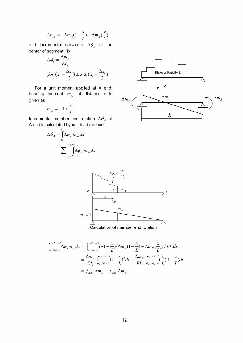
12

)()1(Lxm

Lxmm BAx ∆+−∆−=∆

and incremental curvature xφ∆ at the center of segment i is

)2

()2

( ii

ii

i

xx

xxxxxfor

EIm

∆+≤≤

∆−

∆=∆φ

For a unit moment applied at A end,

bending moment uxm at distance x is given as

Lxmux +−= 1

Incremental member end rotation Aθ∆ at A end is calculated by unit load method:

dxm

dxm

uxi

xx

xxx

ux

L

xA

ii

ii

∑ ∫

∫∆+

∆−

∆=

∆=∆

2/

2/

0

φ

φθ

BABiAAAi

xx

xxi

Bxx

xxi

A

xx

xx iBAux

xx

xx x

mfmf

dxLx

Lx

EImdx

Lx

EIm

dxEILxm

Lxm

Lxdxm

ii

ii

ii

ii

ii

ii

ii

ii

∆+∆=

−∆

−−∆

=

∆+−∆+−=∆

∫∫

∫∫∆+

∆−

∆+

∆−

∆+

∆−

∆+

∆−

2/

2/

2/

2/

2

2/

2/

2/

2/

)1)(()1(

/)}()1(){1(φ

1Am =

A Bi

xx

i

mEI

φ ∆∆ =

ixix∆

uxm

Calculation of member end rotation

Flexural Rigidity EI

Bm∆Am∆

x

xm∆

L

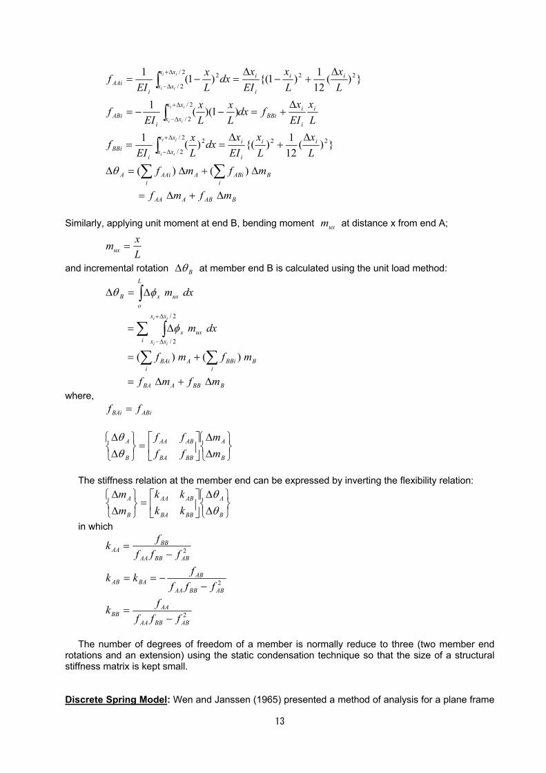
13

})(121){()(1

)1)((1

})(121)1{()1(1

222/

2/

2

2/

2/

222/

2/

2

Lx

Lx

EIx

dxLx

EIf

Lx

EIx

fdxLx

Lx

EIf

Lx

Lx

EIx

dxLx

EIf

ii

i

ixx

xxi

BBi

i

i

iBBi

xx

xxi

ABi

ii

i

ixx

xxi

AAi

ii

ii

ii

ii

ii

ii

∆+

∆==

∆+=−−=

∆+−

∆=−=

∫

∫

∫

∆+

∆−

∆+

∆−

∆+

∆−

BABAAA

Bi

ABiAi

AAiA

mfmf

mfmf

∆+∆=

∆+∆=∆ ∑∑ )()(θ

Similarly, applying unit moment at end B, bending moment uxm at distance x from end A;

Lxmux =

and incremental rotation Bθ∆ at member end B is calculated using the unit load method:

BBBABA

iBBBiA

iBAi

uxi

xx

xxx

ux

L

oxB

mfmf

mfmf

dxm

dxm

ii

ii

∆+∆=

+=

∆=

∆=∆

∑∑

∑ ∫

∫∆+

∆−

)()(

2/

2/

φ

φθ

where, ABiBAi ff =

∆∆

=

∆∆

B

A

BBBA

ABAA

B

A

mm

ffff

θθ

The stiffness relation at the member end can be expressed by inverting the flexibility relation:

∆∆

=

∆∆

B

A

BBBA

ABAA

B

A

kkkk

mm

θθ

in which

2

2

2

ABBBAA

AABB

ABBBAA

ABBAAB

ABBBAA

BBAA

ffffk

ffffkk

ffffk

−=

−−==

−=

The number of degrees of freedom of a member is normally reduce to three (two member end

rotations and an extension) using the static condensation technique so that the size of a structural stiffness matrix is kept small. Discrete Spring Model: Wen and Janssen (1965) presented a method of analysis for a plane frame

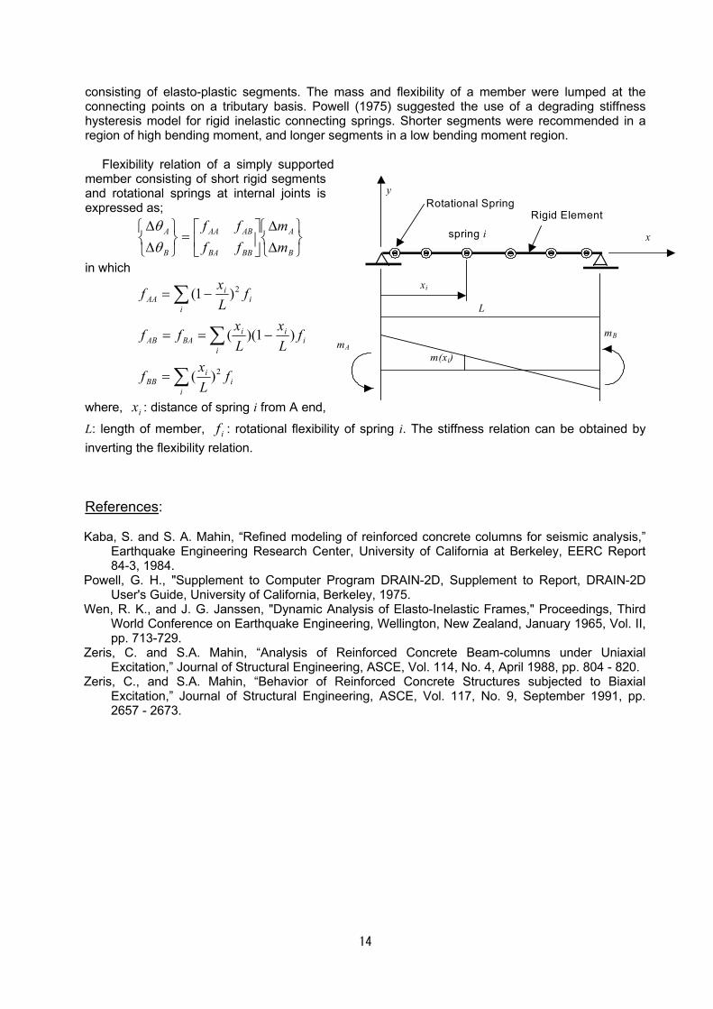
14

consisting of elasto-plastic segments. The mass and flexibility of a member were lumped at the connecting points on a tributary basis. Powell (1975) suggested the use of a degrading stiffness hysteresis model for rigid inelastic connecting springs. Shorter segments were recommended in a region of high bending moment, and longer segments in a low bending moment region.

Flexibility relation of a simply supported member consisting of short rigid segments and rotational springs at internal joints is expressed as;

∆∆

=

∆∆

B

A

BBBA

ABAA

B

A

mm

ffff

θθ

in which

ii

iBB

ii

iiBAAB

ii

iAA

fLxf

fLx

Lxff

fLxf

2

2

)(

)1)((

)1(

∑

∑

∑

=

−==

−=

where, ix : distance of spring i from A end,

L: length of member, if : rotational flexibility of spring i. The stiffness relation can be obtained by inverting the flexibility relation. References:

Kaba, S. and S. A. Mahin, “Refined modeling of reinforced concrete columns for seismic analysis,”

Earthquake Engineering Research Center, University of California at Berkeley, EERC Report 84-3, 1984.

Powell, G. H., "Supplement to Computer Program DRAIN-2D, Supplement to Report, DRAIN-2D User's Guide, University of California, Berkeley, 1975.

Wen, R. K., and J. G. Janssen, "Dynamic Analysis of Elasto-Inelastic Frames," Proceedings, Third World Conference on Earthquake Engineering, Wellington, New Zealand, January 1965, Vol. II, pp. 713-729.

Zeris, C. and S.A. Mahin, “Analysis of Reinforced Concrete Beam-columns under Uniaxial Excitation,” Journal of Structural Engineering, ASCE, Vol. 114, No. 4, April 1988, pp. 804 - 820.

Zeris, C., and S.A. Mahin, “Behavior of Reinforced Concrete Structures subjected to Biaxial Excitation,” Journal of Structural Engineering, ASCE, Vol. 117, No. 9, September 1991, pp. 2657 - 2673.

Rotational Spring Rigid Element

x

y

L

xi

spring i

mA m(xi)

mB

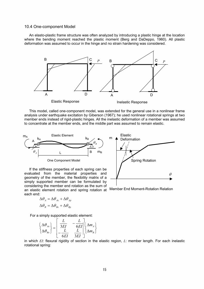
15

10.4 One-component Model

An elasto-plastic frame structure was often analyzed by introducing a plastic hinge at the location where the bending moment reached the plastic moment (Berg and DaDeppo, 1960). All plastic deformation was assumed to occur in the hinge and no strain hardening was considered.

This model, called one-component model, was extended for the general use in a nonlinear frame

analysis under earthquake excitation by Giberson (1967); he used nonlinear rotational springs at two member ends instead of rigid-plastic hinges. All the inelastic deformation of a member was assumed to concentrate at the member ends, and the middle part was assumed to remain elastic.

If the stiffness properties of each spring can be

evaluated from the material properties and geometry of the member, the flexibility matrix of a simply supported member can be formulated by considering the member end rotation as the sum of an elastic element rotation and spring rotation at each end:

BpBeB

ApAeA

θθθ

θθθ

∆+∆=∆

∆+∆=∆

For a simply supported elastic element:

∆∆

−

−=

∆∆

B

A

Be

Ae

mm

EIL

EIL

EIL

EIL

36

63θθ

in which EI: flexural rigidity of section in the elastic region, L: member length. For each inelastic rotational spring:

A

B C

D

Elastic Response

P

A

B C

D

Inelastic Response

P

One Component Model

mA

mBAθ

A

B

kA kBElastic Element

Bθ

L

θ

mElasticDeformation

Spring Rotation

Member End Moment-Rotation Relation

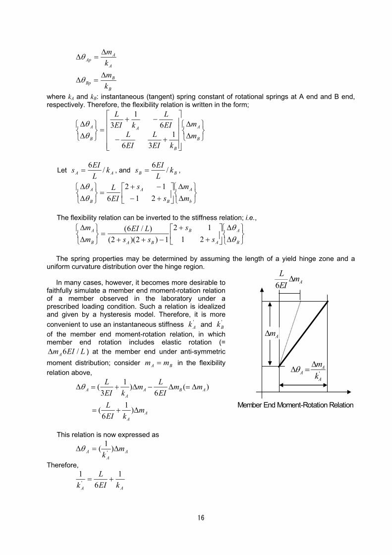
16

B

BBp

A

AAp

kmkm

∆=∆

∆=∆

θ

θ

where kA and kB: instantaneous (tangent) spring constant of rotational springs at A end and B end, respectively. Therefore, the flexibility relation is written in the form;

∆∆

+−

−+=

∆∆

B

A

B

A

B

A

mm

kEIL

EIL

EIL

kEIL

136

61

3θθ

Let AA kLEIs /6

= , and BB kLEIs /6

= ,

∆∆

+−−+

=

∆∆

b

A

B

A

B

A

mm

ss

EIL

2112

6θθ

The flexibility relation can be inverted to the stiffness relation; i.e.,

∆∆

+

+−++

=

∆∆

B

A

A

B

BAB

A

ss

ssLEI

mm

θθ

2112

1)2)(2()/6(

The spring properties may be determined by assuming the length of a yield hinge zone and a

uniform curvature distribution over the hinge region.

In many cases, however, it becomes more desirable to faithfully simulate a member end moment-rotation relation of a member observed in the laboratory under a prescribed loading condition. Such a relation is idealized and given by a hysteresis model. Therefore, it is more convenient to use an instantaneous stiffness '

Ak and 'Bk

of the member end moment-rotation relation, in which member end rotation includes elastic rotation (=

LEImA /6∆ ) at the member end under anti-symmetric moment distribution; consider BA mm = in the flexibility relation above,

1( ) ( )3 6

1( )6

A A B AA

AA

L Lm m mEI k EIL mEI k

θ∆ = + ∆ − ∆ = ∆

= + ∆

This relation is now expressed as

AA

A mk

∆=∆ )1( 'θ

Therefore,

AA kEI

Lk

16

1' +=

'A

AA

mk

θ ∆∆ =

Am∆

AmEIL

∆6

Member End Moment-Rotation Relation

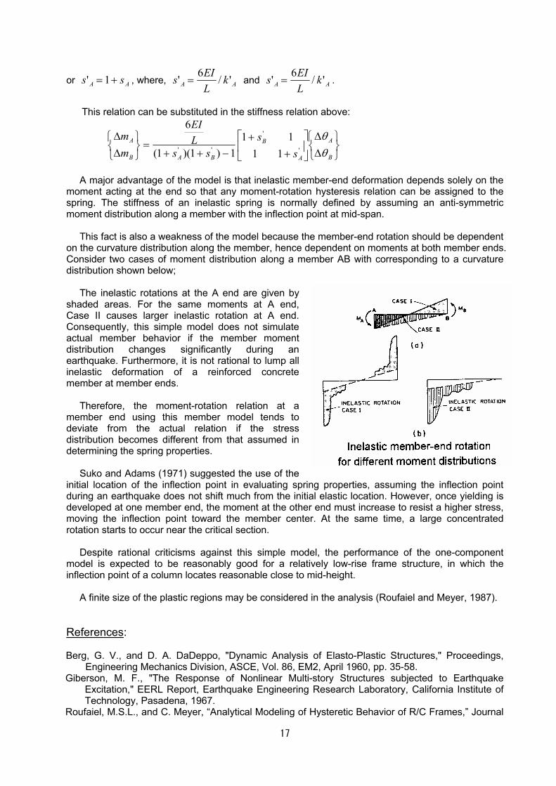
17

or AA ss += 1' , where, AA kLEIs '/6' = and AA k

LEIs '/6' = .

This relation can be substituted in the stiffness relation above:

∆∆

++

−++=

∆∆

B

A

A

B

BAB

A

ss

ssLEI

mm

θθ

'

'

'' 1111

1)1)(1(

6

A major advantage of the model is that inelastic member-end deformation depends solely on the

moment acting at the end so that any moment-rotation hysteresis relation can be assigned to the spring. The stiffness of an inelastic spring is normally defined by assuming an anti-symmetric moment distribution along a member with the inflection point at mid-span.

This fact is also a weakness of the model because the member-end rotation should be dependent

on the curvature distribution along the member, hence dependent on moments at both member ends. Consider two cases of moment distribution along a member AB with corresponding to a curvature distribution shown below;

The inelastic rotations at the A end are given by shaded areas. For the same moments at A end, Case II causes larger inelastic rotation at A end. Consequently, this simple model does not simulate actual member behavior if the member moment distribution changes significantly during an earthquake. Furthermore, it is not rational to lump all inelastic deformation of a reinforced concrete member at member ends.

Therefore, the moment-rotation relation at a member end using this member model tends to deviate from the actual relation if the stress distribution becomes different from that assumed in determining the spring properties.

Suko and Adams (1971) suggested the use of the initial location of the inflection point in evaluating spring properties, assuming the inflection point during an earthquake does not shift much from the initial elastic location. However, once yielding is developed at one member end, the moment at the other end must increase to resist a higher stress, moving the inflection point toward the member center. At the same time, a large concentrated rotation starts to occur near the critical section.

Despite rational criticisms against this simple model, the performance of the one-component model is expected to be reasonably good for a relatively low-rise frame structure, in which the inflection point of a column locates reasonable close to mid-height.

A finite size of the plastic regions may be considered in the analysis (Roufaiel and Meyer, 1987). References: Berg, G. V., and D. A. DaDeppo, "Dynamic Analysis of Elasto-Plastic Structures," Proceedings,

Engineering Mechanics Division, ASCE, Vol. 86, EM2, April 1960, pp. 35-58. Giberson, M. F., "The Response of Nonlinear Multi-story Structures subjected to Earthquake

Excitation," EERL Report, Earthquake Engineering Research Laboratory, California Institute of Technology, Pasadena, 1967.

Roufaiel, M.S.L., and C. Meyer, “Analytical Modeling of Hysteretic Behavior of R/C Frames,” Journal

Inelastic member-end rotation for different moment distributions

18

of Structural Engineering, ASCE, Vol. 113, No. 3, March 1987, pp. 429-444. Suko, M., and P. F. Adams, "Dynamic Analysis of Multi-bay Multi-story Frames," Journal, Structural

Division, ASCE, Vol. 97, No. ST10, October 1971, pp. 2519-2533.

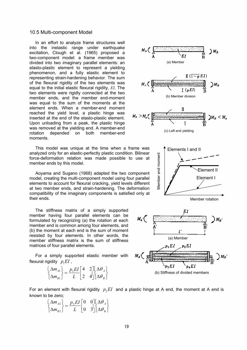
19

10.5 Multi-component Model

In an effort to analyze frame structures well into the inelastic range under earthquake excitation, Clough et al. (1965) proposed a two-component model: a frame member was divided into two imaginary parallel elements: an elasto-plastic element to represent a yielding phenomenon, and a fully elastic element to representing strain-hardening behavior. The sum of the flexural rigidity of the two elements was equal to the initial elastic flexural rigidity, EI. The two elements were rigidly connected at the two member ends, and the member end-moment was equal to the sum of the moments at the element ends. When a member-end moment reached the yield level, a plastic hinge was inserted at the end of the elasto-plastic element. Upon unloading from a peak, the plastic hinge was removed at the yielding end. A member-end rotation depended on both member-end moments.

This model was unique at the time when a frame was

analyzed only for an elastic-perfectly plastic condition. Bilinear force-deformation relation was made possible to use at member ends by this model.

Aoyama and Sugano (1968) adapted the two component

model, creating the multi-component model using four parallel elements to account for flexural cracking, yield levels different at two member ends, and strain-hardening. The deformation compatibility of the imaginary components is satisfied only at their ends.

The stiffness matrix of a simply supported member having four parallel elements can be formulated by recognizing (a) the rotation at each member end is common among four elements, and (b) the moment at each end is the sum of moment resisted by four elements. In other words, the member stiffness matrix is the sum of stiffness matrices of four parallel elements.

For a simply supported elastic member with

flexural rigidity 1p EI ,

∆∆

=

∆∆

B

A

B

A

LEIp

mm

θθ

42241

1

1

For an element with flexural rigidity 2p EI and a plastic hinge at A end, the moment at A end is known to be zero;

∆∆

=

∆∆

B

A

B

A

LEIp

mm

θθ

30002

2

2

Member Rotation

(a) Member

(b) Member division

(c) Left end yielding

Element I

Element II

Elements I and II

Member rotation

Mem

ber e

nd m

omen

t

(a) Member

(b) Stiffness of divided members

20

Similarly, for an element with flexural rigidity 3p EI and a plastic hinge at B end;

∆∆

=

∆∆

B

A

B

A

LEIp

mm

θθ

00033

3

3

For an element with plastic hinges at the two ends, the stiffness matrix is zero;

∆∆

=

∆∆

B

A

B

A

mm

θθ

0000

4

4

From the equilibrium of forces;

4321

4321

BBBBB

AAAAA

mmmmmmmmmm

∆+∆+∆+∆=∆∆+∆+∆+∆=∆

Therefore, the stiffness matrix of a simply supported member is written as follows;

∆∆

+

+=

∆∆

B

A

B

A

pppppp

LEI

mm

θθ

)34(22)34(

211

131

Note that 032 =⋅ pp ; an element having a plastic hinge at A end and another element having a

plastic hinge at B end cannot exist simultaneously; i.e., either 2p or 3p or both should be zero at a stage.

The multi-component model appears to have a merit; rotation at one end of a member depends

on both member-end moments. In other words, the moment distribution along a member can be approximately reflected in the analysis. However, the stiffness of the multi-parallel components must be evaluated under a certain assumed moment distribution. Therefore, the stiffness parameters are valid only under such a moment distribution, and are bound to be approximate when the moment distribution becomes drastically different in the analysis.

Giberson (1967) discussed the advantage and disadvantage of the one-component and the two-component models, and concluded that the one-component model was more versatile than the two-component model because the two-component model was restricted to the bilinear hysteresis characteristics.

The ratios p's of element stiffness may be varied with damage if a more general hysteresis relation is desired for a member. Takizawa (1976) suggested the ratios p's be determined as a function of member end stiffness under an anti-symmetric moment distribution. The flexibility matrix including shear deformation is given below:

∆∆

=

∆∆

B

A

B

A

mm

ffff

2221

1211

θθ

where, for 2( 0)B Af f p< = :

B

B

BA

ff

fff

fff

γγ

γγ

γγγ

γ

212

21)1(

)2)(21()1(

23

22

2112

2

11

++

=

+−

−==

++−

++

=

and for 3( 0)B Af f p> = ,

21

BA

A

A

fff

fff

ff

γγγγ

γγ

γγ

++

++−

=

+−

−==

++

=

23

)2)(21()1(

21)1(

212

2

22

2112

11

γ : parameter describing the relative contribution of shear deformation (= 26 /EI GALκ ). Flexibility parameters Af and Bf are given by a hysteresis model at member ends A and B;

B

BB

A

AA

mf

mf

∆∆

=

∆∆

=

θ

θ

under anti-symmetric bending moment distribution.

The axial load-bending moment interaction may be approximated by changing the yield moment level of elements as a function of existing axial load. References: Aoyama, H., and T. Sugano, "A Generalized Inelastic Analysis of Reinforced Concrete Structures

based on the Tests of Members," Recent Researches of Structural Mechanics, Contribution in Honor of the 60-th Birthday of Professor Y. Tsuboi, Uno Shoten, Tokyo, 1968, pp. 15-30.

Clough, R. W., K. L. Benuska and E. L. Wilson, "Inelastic Earthquake response of tall buildings," Proceedings, Third World Conference on Earthquake Engineering, New Zealand, Vol. II, Session II, 1965, pp. 68-89.

Giberson, M. F., "The Response of Nonlinear Multi-story Structures subjected to Earthquake Excitation," EERL Report, Earthquake Engineering Research Laboratory, California Institute of Technology, 1967.

Takizawa, T., "Notes on Some Basic Problems in Inelastic Analysis of Planar R/C Structures (Part 1)," Transactions, Architectural Institute of Japan, No. 240, February 1976, pp. 51-62.

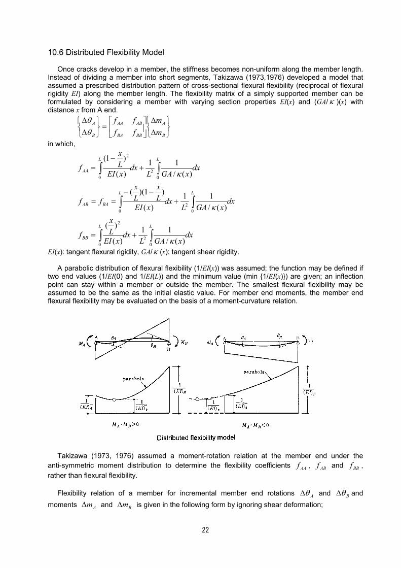
22

10.6 Distributed Flexibility Model

Once cracks develop in a member, the stiffness becomes non-uniform along the member length. Instead of dividing a member into short segments, Takizawa (1973,1976) developed a model that assumed a prescribed distribution pattern of cross-sectional flexural flexibility (reciprocal of flexural rigidity EI) along the member length. The flexibility matrix of a simply supported member can be formulated by considering a member with varying section properties EI(x) and (GA/κ )(x) with distance x from A end.

∆∆

=

∆∆

B

A

BBBA

ABAA

B

A

mm

ffff

θθ

in which,

dxxGAL

dxxEI

Lx

f

dxxGAL

dxxEI

Lx

Lx

ff

dxxGAL

dxxEILx

f

LL

BB

LL

BAAB

LL

AA

∫∫

∫∫

∫∫

+=

+−−

==

+−

=

02

0

2

02

0

02

0

2

)(/11

)(

)(

)(/11

)(

)1)((

)(/11

)(

)1(

κ

κ

κ

EI(x): tangent flexural rigidity, GA/κ (x): tangent shear rigidity.

A parabolic distribution of flexural flexibility (1/EI(x)) was assumed; the function may be defined if two end values (1/EI(0) and 1/EI(L)) and the minimum value (min {1/EI(x)}) are given; an inflection point can stay within a member or outside the member. The smallest flexural flexibility may be assumed to be the same as the initial elastic value. For member end moments, the member end flexural flexibility may be evaluated on the basis of a moment-curvature relation.

Takizawa (1973, 1976) assumed a moment-rotation relation at the member end under the anti-symmetric moment distribution to determine the flexibility coefficients AAf , ABf and BBf , rather than flexural flexibility.

Flexibility relation of a member for incremental member end rotations Aθ∆ and Bθ∆ and moments Am∆ and Bm∆ is given in the following form by ignoring shear deformation;

23

∆∆

−−

+++

−

++

−−−

+=

∆∆

B

A

ABoA

BABBA

ABBAAB

oBA

B

A

mm

fffffff

fffffff

32

32

2)(

32

2)(

32

θθ

in which of : member end flexibility at the initial elastic stage (= L / 6 EI).

Member end flexibility Af or Bf was determined as an incremental member end rotation to moment ratio under the anti-symmetric bending moment distribution with the same member end moments of amplitude Am or Bm acting at the two ends. The curvature was assumed to distribute along the member length in a parabolic form with the initial elastic value at the mid-span. Normally, this flexibility is given by a hysteresis model.

The interacting element ABf is defined as

)sgn())(( BAoBoAAB mmfffff −−=

This is an interesting concept in analyzing an inelastic member. However, the parabolic flexibility distribution may not describe the actual concentration of deformation at critical section (normally at member ends) due to flexural yielding and deformation attributable to slippage of longitudinal reinforcement within a beam-column connection. The usage of inelastic springs at locations of concentrated deformation in conjunction with this model may be a useful solution. References: Takizawa, H., "Analysis of Reinforced Concrete Buildings under Strong Earthquake Motion (in

Japanese)," Concrete Journal, Japan Concrete Institute, Vol. 11, No. 2, February 1973, pp. 10-21.

Takizawa, H., "Notes on Some Basic Problems in Inelastic Analysis of Planar R/C Structures (Part 1)," Transactions, Architectural Institute of Japan, No. 240, February 1976, pp. 51-62.

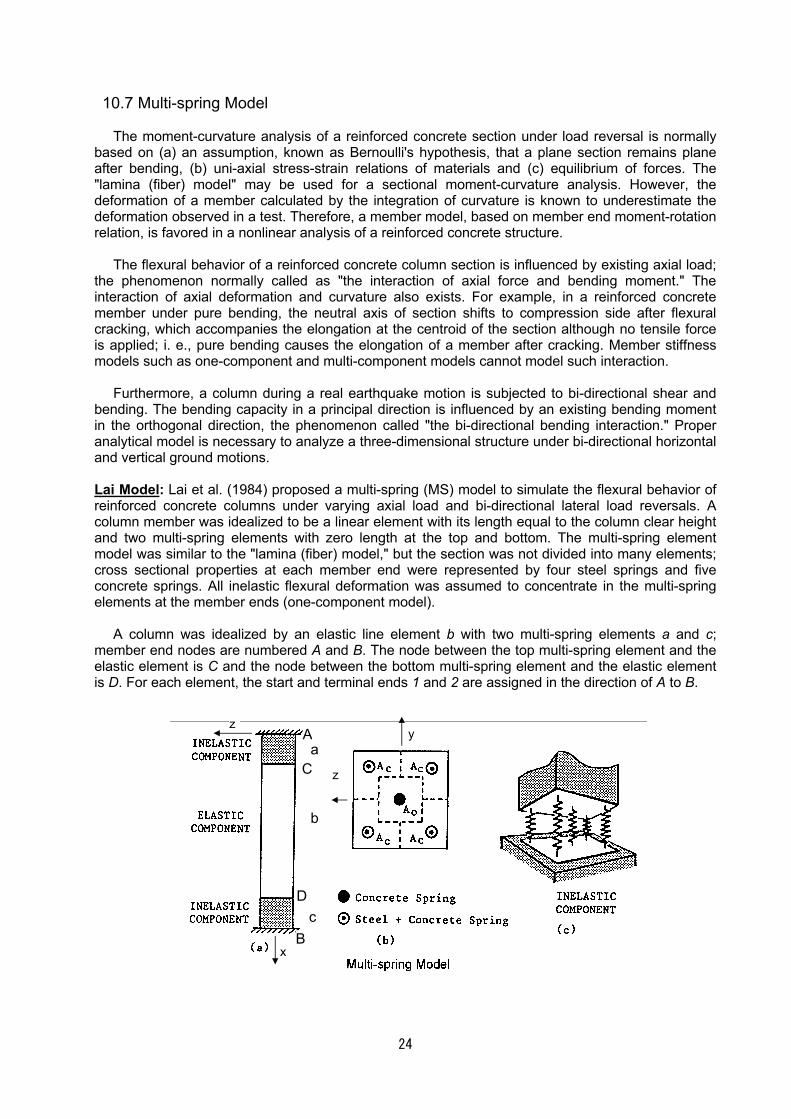
24

10.7 Multi-spring Model

The moment-curvature analysis of a reinforced concrete section under load reversal is normally based on (a) an assumption, known as Bernoulli's hypothesis, that a plane section remains plane after bending, (b) uni-axial stress-strain relations of materials and (c) equilibrium of forces. The "lamina (fiber) model" may be used for a sectional moment-curvature analysis. However, the deformation of a member calculated by the integration of curvature is known to underestimate the deformation observed in a test. Therefore, a member model, based on member end moment-rotation relation, is favored in a nonlinear analysis of a reinforced concrete structure.

The flexural behavior of a reinforced concrete column section is influenced by existing axial load; the phenomenon normally called as "the interaction of axial force and bending moment." The interaction of axial deformation and curvature also exists. For example, in a reinforced concrete member under pure bending, the neutral axis of section shifts to compression side after flexural cracking, which accompanies the elongation at the centroid of the section although no tensile force is applied; i. e., pure bending causes the elongation of a member after cracking. Member stiffness models such as one-component and multi-component models cannot model such interaction.

Furthermore, a column during a real earthquake motion is subjected to bi-directional shear and bending. The bending capacity in a principal direction is influenced by an existing bending moment in the orthogonal direction, the phenomenon called "the bi-directional bending interaction." Proper analytical model is necessary to analyze a three-dimensional structure under bi-directional horizontal and vertical ground motions. Lai Model: Lai et al. (1984) proposed a multi-spring (MS) model to simulate the flexural behavior of reinforced concrete columns under varying axial load and bi-directional lateral load reversals. A column member was idealized to be a linear element with its length equal to the column clear height and two multi-spring elements with zero length at the top and bottom. The multi-spring element model was similar to the "lamina (fiber) model," but the section was not divided into many elements; cross sectional properties at each member end were represented by four steel springs and five concrete springs. All inelastic flexural deformation was assumed to concentrate in the multi-spring elements at the member ends (one-component model).

A column was idealized by an elastic line element b with two multi-spring elements a and c; member end nodes are numbered A and B. The node between the top multi-spring element and the elastic element is C and the node between the bottom multi-spring element and the elastic element is D. For each element, the start and terminal ends 1 and 2 are assigned in the direction of A to B.

A

B

C

D

a

b

c

y

z

x

z

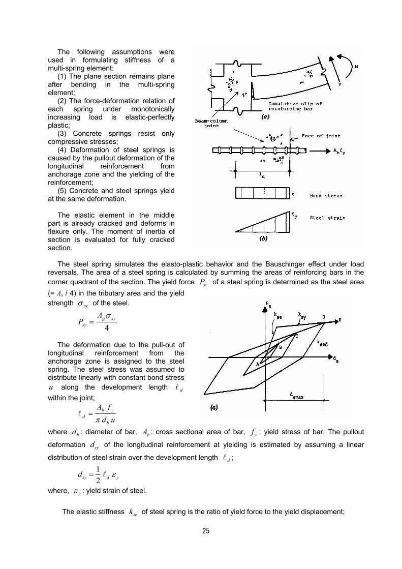
25

The following assumptions were used in formulating stiffness of a multi-spring element:

(1) The plane section remains plane after bending in the multi-spring element;

(2) The force-deformation relation of each spring under monotonically increasing load is elastic-perfectly plastic;

(3) Concrete springs resist only compressive stresses;

(4) Deformation of steel springs is caused by the pullout deformation of the longitudinal reinforcement from anchorage zone and the yielding of the reinforcement;

(5) Concrete and steel springs yield at the same deformation.

The elastic element in the middle part is already cracked and deforms in flexure only. The moment of inertia of section is evaluated for fully cracked section.

The steel spring simulates the elasto-plastic behavior and the Bauschinger effect under load

reversals. The area of a steel spring is calculated by summing the areas of reinforcing bars in the corner quadrant of the section. The yield force syP of a steel spring is determined as the steel area (= As / 4) in the tributary area and the yield strength syσ of the steel.

4

sygsy

AP

σ=

The deformation due to the pull-out of

longitudinal reinforcement from the anchorage zone is assigned to the steel spring. The steel stress was assumed to distribute linearly with constant bond stress u along the development length dl within the joint;

ud

fA

b

ybd π=l

where bd : diameter of bar, bA : cross sectional area of bar, yf : yield stress of bar. The pullout

deformation syd of the longitudinal reinforcement at yielding is estimated by assuming a linear

distribution of steel strain over the development length dl ;

12sy d yd ε= l

where, yε : yield strain of steel.

The elastic stiffness sek of steel spring is the ratio of yield force to the yield displacement;

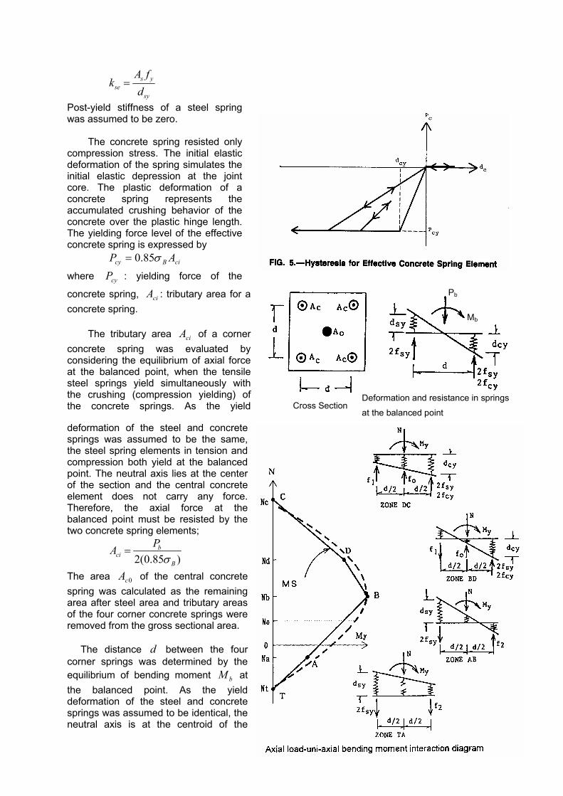
26

s yse

sy

A fk

d=

Post-yield stiffness of a steel spring was assumed to be zero.

The concrete spring resisted only compression stress. The initial elastic deformation of the spring simulates the initial elastic depression at the joint core. The plastic deformation of a concrete spring represents the accumulated crushing behavior of the concrete over the plastic hinge length. The yielding force level of the effective concrete spring is expressed by

ciBcy AP σ85.0=

where cyP : yielding force of the

concrete spring, ciA : tributary area for a concrete spring.

The tributary area ciA of a corner concrete spring was evaluated by considering the equilibrium of axial force at the balanced point, when the tensile steel springs yield simultaneously with the crushing (compression yielding) of the concrete springs. As the yield

deformation of the steel and concrete springs was assumed to be the same, the steel spring elements in tension and compression both yield at the balanced point. The neutral axis lies at the center of the section and the central concrete element does not carry any force. Therefore, the axial force at the balanced point must be resisted by the two concrete spring elements;

2(0.85 )

bci

B

PAσ

=

The area 0cA of the central concrete spring was calculated as the remaining area after steel area and tributary areas of the four corner concrete springs were removed from the gross sectional area.

The distance d between the four corner springs was determined by the equilibrium of bending moment bM at the balanced point. As the yield deformation of the steel and concrete springs was assumed to be identical, the neutral axis is at the centroid of the

Cross Section Deformation and resistance in springs

at the balanced point

Pb

Mb

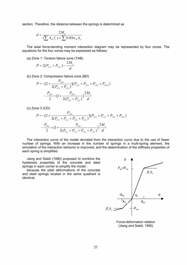
27

section. Therefore, the distance between the springs is determined as

∑ ∑+

=ciBysi

b

AfAM

dσ85.0)(

2

The axial force-bending moment interaction diagram may be represented by four zones. The

equations for the four zonse may be expressed as follows; (a) Zone 1: Tension failure zone (TAB)

dM

PPP yysys

2)(2 31 −+=

(b) Zone 2: Compression failure zone (BD)

02 2 4 4 )

1 3

0 0

1 3

[2 ]( )2( )

2[1 ]

2 2( )

c yc y s y c y s y

s y s y

c y c y y

s y s y

PP P P P P

P P

P P MP P d

= − + + + ++

− + ++

(c) Zone 3 (CD):

02 2 4 4

1 1 3 3

0 0

1 1 3 3

[2 ]( )2( )

2[1 ]

2 2( )

c yc y s y c y s y

s y c y s y c y

c y c y y

s y c y s y c y

PP P P P P

P P P P

P P MP P P P d

= − + + + ++ + +

− + ++ + +

The interaction curve of the model deviated from the interaction curve due to the use of fewer

number of springs. With an increase in the number of springs in a multi-spring element, the simulation of the interaction behavior is improved, and the determination of the stiffness properties of each spring is simplified.

Jiang and Saiidi (1990) proposed to combine the hysteresis properties of the concrete and steel springs in each corner to simplify the model .

because the yield deformations of the concrete and steel springs located in the same quadrant is identical.

Force-deformation relation (Jiang and Saiidi, 1990)

d

F

Fsy+Fcy

-Fsy

dsy

-dsy k1

k2

2ksβ

2ksβ

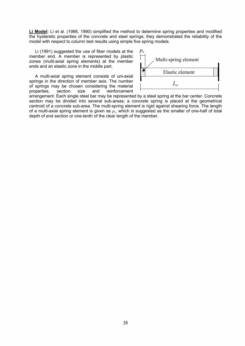
28

Li Model: Li et al. (1988, 1990) simplified the method to determine spring properties and modified the hysteretic properties of the concrete and steel springs; they demonstrated the reliability of the model with respect to column test results using simple five spring models.

Li (1991) suggested the use of fiber models at the member end. A member is represented by plastic zones (multi-axial spring elements) at the member ends and an elastic zone in the middle part.

A multi-axial spring element consists of uni-axial

springs in the direction of member axis. The number of springs may be chosen considering the material properties, section size and reinforcement arrangement. Each single steel bar may be represented by a steel spring at the bar center. Concrete section may be divided into several sub-areas; a concrete spring is placed at the geometrical centroid of a concrete sub-area. The multi-spring element is rigid against shearing force. The length of a multi-axial spring element is given as pz, which is suggested as the smaller of one-half of total depth of end section or one-tenth of the clear length of the member.

Lo

pz

Multi-spring element

Elastic element

29

The axial force fi and deformation di of each axial spring are given as follows;

zii

iii

pdAf

εσ

==

where iσ and iε : stress and strain at spring point i, and iA . area of sub-area i. Multi-linear stress-strain relation may be used for concrete and steel springs. Some adjustment is required for the stress-strain relation of a steel spring to take into account the stiffness degradation, for example, due to the bond slip along the longitudinal reinforcement or the pullout deformation of the longitudinal reinforcement from the anchorage zone. The yield deformation may be increased by a factor κ ;

0.10.1

0.10.1

0.1

≤=

>−

+=

Dhfor

Dhfor

Dh

Dh

o

o

o

o

κ

κ

where ho: shear span, and D: overall depth of section.

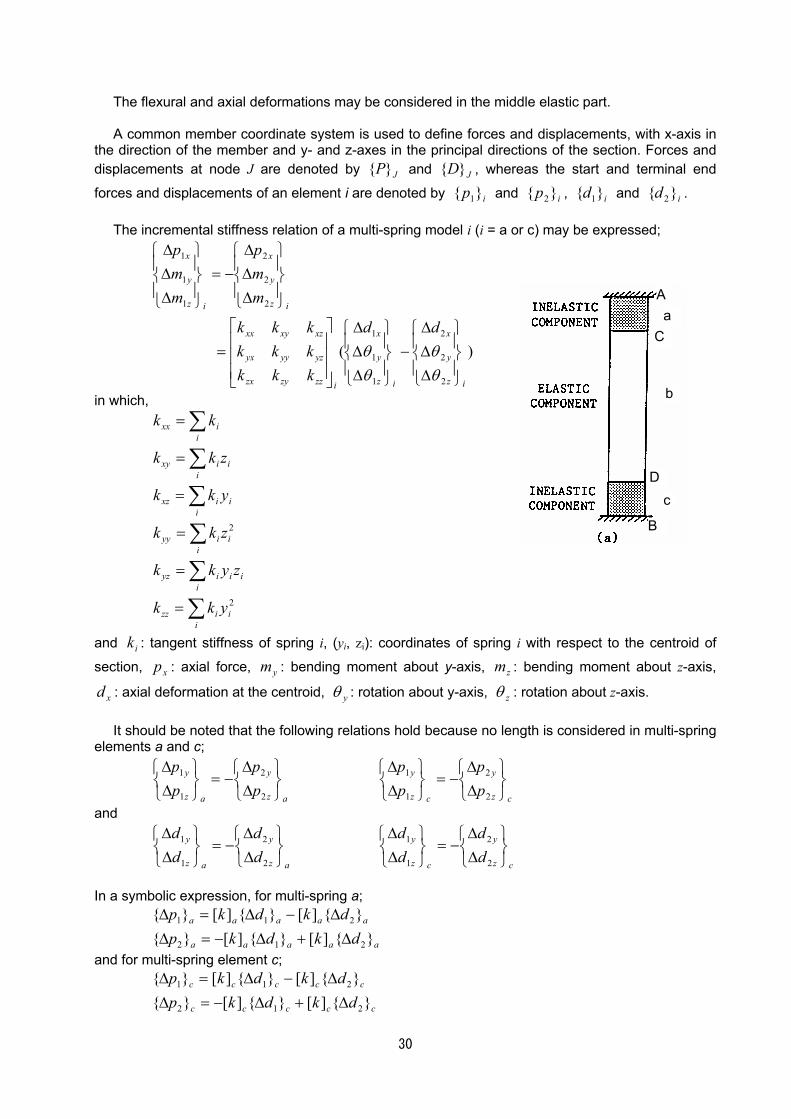
30

The flexural and axial deformations may be considered in the middle elastic part.

A common member coordinate system is used to define forces and displacements, with x-axis in the direction of the member and y- and z-axes in the principal directions of the section. Forces and displacements at node J are denoted by JP}{ and JD}{ , whereas the start and terminal end

forces and displacements of an element i are denoted by ip }{ 1 and ip }{ 2 , id }{ 1 and id }{ 2 .

The incremental stiffness relation of a multi-spring model i (i = a or c) may be expressed;

)(

2

2

2

1

1

1

2

2

2

1

1

1

iz

y

x

iz

y

x

izzzyzx

yzyyyx

xzxyxx

iz

y

x

iz

y

x

dd

kkkkkkkkk

mmp

mmp

∆∆∆

−

∆∆∆

=

∆∆∆

−=

∆∆∆

θθ

θθ

in which,

∑

∑

∑

∑

∑

∑

=

=

=

=

=

=

iiizz

iii

iyz

ii

iyy

ii

ixz

ii

ixy

iixx

ykk

zykk

zkk

ykk

zkk

kk

2

2

and ik : tangent stiffness of spring i, (yi, zi): coordinates of spring i with respect to the centroid of

section, xp : axial force, ym : bending moment about y-axis, zm : bending moment about z-axis,

xd : axial deformation at the centroid, yθ : rotation about y-axis, zθ : rotation about z-axis.

It should be noted that the following relations hold because no length is considered in multi-spring elements a and c;

az

y

az

y

pp

pp

∆∆

−=

∆∆

2

2

1

1 cz

y

cz

y

pp

pp

∆∆

−=

∆∆

2

2

1

1

and

az

y

az

y

dd

dd

∆∆

−=

∆∆

2

2

1

1 cz

y

cz

y

dd

dd

∆∆

−=

∆∆

2

2

1

1

In a symbolic expression, for multi-spring a;

aaaaa

aaaaa

dkdkpdkdkp

}{][}{][}{}{][}{][}{

212

211

∆+∆−=∆∆−∆=∆

and for multi-spring element c;

ccccc

ccccc

dkdkpdkdkp

}{][}{][}{}{][}{][}{

212

211

∆+∆−=∆∆−∆=∆

A

C

D

a

b

c

B

31

For an elastic element of length L, flexural rigidity EI, axial rigidity EA, and shear rigidity GA/κ, a

stiffness relation can be formulated in the form:

bbbbb

bbbbb

dkdkpdkdkp

}{][}{][}{}{][}{][}{

2221212

2121111

∆+∆=∆∆+∆=∆

where, bkp }{ and bkd }{ at k-end are Tzkzkykykxk mpmpp },,,,{ and T

zkzkykykxk ddd },,,,{ θθ .

The compatibility of displacements at nodes:

cbD

baC

cB

aA

ddDddD

dDdD

}{}{}{}{}{}{

}{}{}{}{

12

12

2

1

∆=∆=∆∆=∆=∆

∆=∆∆=∆

Equilibrium of external forces and the sum of internal element end forces at a node;

cbD

baC

cB

aA

ppPppP

pPpP

}{}{}{}{}{}{

}{}{}{}{

12

12

2

1

∆+∆=∆∆+∆=∆

∆=∆∆=∆

Special care must be exercised in formulating a member stiffness matrix with four nodes (A, B, C

and D) to include the following conditions; (a) for displacements:

cz

y

cz

y

Bz

y

Dz

y

az

y

az

y

Cz

y

Az

y

dd

dd

DD

DD

dd

dd

DD

DD

∆∆

=

∆∆

=

∆∆

=

∆∆

∆∆

=

∆∆

=

∆∆

=

∆∆

2

2

1

1

2

2

1

1

and (b) for forces:

az

y

az

y

pp

pp

∆∆

−=

∆∆

2

2

1

1 cz

y

cz

y

pp

pp

∆∆

−=

∆∆

2

2

1

1

References:

Lai, S.-S., G. T. Will and S. Otani, "Model for Inelastic Bi-axial Bending of Concrete Member,"

Journal, Structural Division, ASCE, Vol. 110, No. ST11, November 1984, pp. 2563-2584. Jiang, Y., and S. M. Saiidi, "Four-Spring Element for Cyclic Response of R/C Columns," Journal,

Structural Engineering Division, ASCE, Vol. 116, No. ST4, April 1990, pp. 1018-1029. Li, K.-N., S. Otani and H. Aoyama, "Reinforced Concrete Columns under Varying Axial Load and

B-directional Lateral Load Reversals," Proceedings, Ninth World Conference on Earthquake Engineering, Tokyo-Kyoto, August 1988, Vol. VIII, pp. 537-542.

Li, K.-N., S. Otani and H. Aoyama, "Study on Reinforced Concrete Columns subjected to Varying Axial Load and Bi-directional Horizontal Earthquake Loads (in Japanese)," Report, Aoyama Laboratory, Department of Architecture, Faculty of Engineering, University of Tokyo, March 1990.

Li, Kang-Ning, S. Otani and H. Aoyama, “R/C Columns under Axial and Bi-directional Lateral Loads,” Proceedings, Mechanics Computing in 1990’s and Beyond, ASCE, Vol. 2, Structural and Material Mechanics, May 1991, pp. 681 - 685.

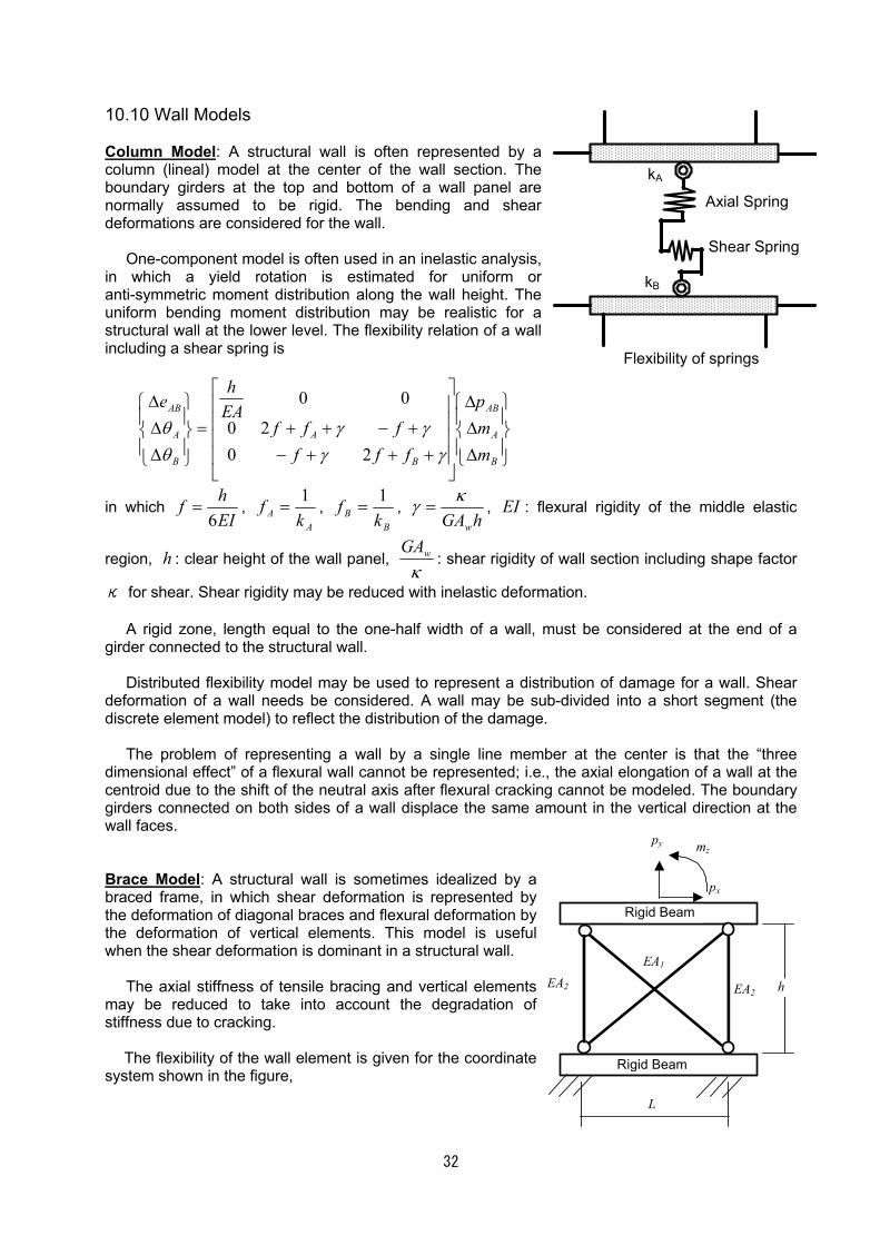
32

10.10 Wall Models Column Model: A structural wall is often represented by a column (lineal) model at the center of the wall section. The boundary girders at the top and bottom of a wall panel are normally assumed to be rigid. The bending and shear deformations are considered for the wall.

One-component model is often used in an inelastic analysis, in which a yield rotation is estimated for uniform or anti-symmetric moment distribution along the wall height. The uniform bending moment distribution may be realistic for a structural wall at the lower level. The flexibility relation of a wall including a shear spring is

∆∆∆

+++−+−++=

∆∆∆

B

A

AB

B

A

B

A

AB

mmp

ffffff

EAh

e

γγγγ

θθ

2020

00

in which EIhf

6= ,

AA k

f 1= ,

BB k

f 1= ,

hGAw

κγ = , EI : flexural rigidity of the middle elastic

region, h : clear height of the wall panel, κ

wGA: shear rigidity of wall section including shape factor

κ for shear. Shear rigidity may be reduced with inelastic deformation.

A rigid zone, length equal to the one-half width of a wall, must be considered at the end of a girder connected to the structural wall.

Distributed flexibility model may be used to represent a distribution of damage for a wall. Shear deformation of a wall needs be considered. A wall may be sub-divided into a short segment (the discrete element model) to reflect the distribution of the damage.

The problem of representing a wall by a single line member at the center is that the “three dimensional effect” of a flexural wall cannot be represented; i.e., the axial elongation of a wall at the centroid due to the shift of the neutral axis after flexural cracking cannot be modeled. The boundary girders connected on both sides of a wall displace the same amount in the vertical direction at the wall faces. Brace Model: A structural wall is sometimes idealized by a braced frame, in which shear deformation is represented by the deformation of diagonal braces and flexural deformation by the deformation of vertical elements. This model is useful when the shear deformation is dominant in a structural wall.

The axial stiffness of tensile bracing and vertical elements may be reduced to take into account the degradation of stiffness due to cracking.

The flexibility of the wall element is given for the coordinate

system shown in the figure,

kA

kB

Axial Spring

Shear Spring

Flexibility of springs

h

Rigid Beam

Rigid Beam

L

px

py mz

EA1 EA2 EA2

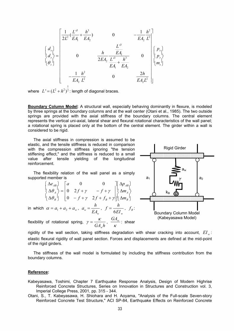
33

3 3 2

2 21 2 2

3

13 3

2

1 22

2 22 2

1 ' 1( ) 02

'

0 0'2

1 20

x x

y y

z z

L h hL EA EA EA L

Ld ph EAd p

L hEAmEA EA

h hEA L EA L

θ

+ −

= +

−

where 1

2 2 2' ( )L L h= + : length of diagonal braces.

Boundary Column Model: A structural wall, especially behaving dominantly in flexure, is modeled by three springs at the boundary columns and at the wall center (Otani et al., 1985). The two outside springs are provided with the axial stiffness of the boundary columns. The central element represents the vertical uni-axial, lateral shear and flexural rotational characteristics of the wall panel; a rotational spring is placed only at the bottom of the central element. The girder within a wall is considered to be rigid.

The axial stiffness in compression is assumed to be elastic, and the tensile stiffness is reduced in comparison with the compression stiffness ignoring "the tension stiffening effect," and the stiffness is reduced to a small value after tensile yielding of the longitudinal reinforcement.

The flexibility relation of the wall panel as a simply supported member is

∆∆∆

+++−+−+=

∆∆∆

B

A

AB

BB

A

AB

mmp

fffff

ae

γγγγ

θθ

2020

00

in which waaa ++= 21α , ww

haEA

= , wEI

hf6

= , Bf :

flexibility of rotational spring, hGAw

κγ = , κ

wGA: shear

rigidity of the wall section, taking stiffness degradation with shear cracking into account, wEI : elastic flexural rigidity of wall panel section. Forces and displacements are defined at the mid-point of the rigid girders.

The stiffness of the wall model is formulated by including the stiffness contribution from the boundary columns. Reference: Kabeyasawa, Toshimi, Chapter 7 Earthquake Response Analysis, Design of Modern Highrise

Reinforced Concrete Structures, Series on Innovation in Structures and Construction vol. 3, Imperial College Press, 2001, pp. 315 - 344.

Otani, S., T. Kabeyasawa, H. Shiohara and H. Aoyama, "Analysis of the Full-scale Seven-story Reinforced Concrete Test Structure," ACI SP-84, Earthquake Effects on Reinforced Concrete

kB

a1 a2

aw

γ

Rigid Girder

Boundary Column Model (Kabeyasawa Model)

34

Structure, US-Japan Research, American Concrete Institute, Detroit, 1985, pp. 203-239. Vulcano, A., and V. V. Bertero, “Analytical Models for Predicting the Lateral Response of RC Shear

Walls,” University of California at Berkeley, Earthquake Engineering Research Center, Report No. EERC 87-19, 1987.

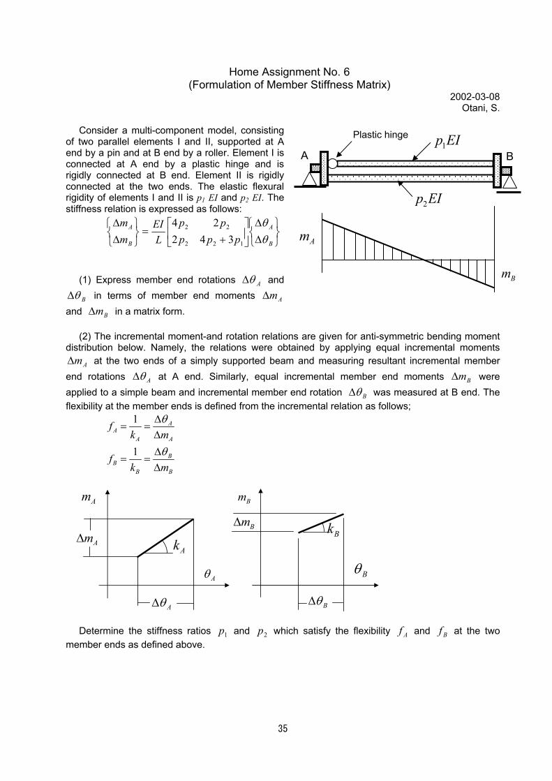
35

Home Assignment No. 6 (Formulation of Member Stiffness Matrix)

2002-03-08 Otani, S.

Consider a multi-component model, consisting

of two parallel elements I and II, supported at A end by a pin and at B end by a roller. Element I is connected at A end by a plastic hinge and is rigidly connected at B end. Element II is rigidly connected at the two ends. The elastic flexural rigidity of elements I and II is p1 EI and p2 EI. The stiffness relation is expressed as follows:

∆∆

+

=

∆∆

B

A

B

A

ppppp

LEI

mm

θθ

122

22

34224

(1) Express member end rotations Aθ∆ and

Bθ∆ in terms of member end moments Am∆ and Bm∆ in a matrix form.

(2) The incremental moment-and rotation relations are given for anti-symmetric bending moment

distribution below. Namely, the relations were obtained by applying equal incremental moments Am∆ at the two ends of a simply supported beam and measuring resultant incremental member

end rotations Aθ∆ at A end. Similarly, equal incremental member end moments Bm∆ were applied to a simple beam and incremental member end rotation Bθ∆ was measured at B end. The flexibility at the member ends is defined from the incremental relation as follows;

1

1

AA

A A

BB

B B

fk m

fk m

θ

θ

∆= =

∆∆

= =∆

Aθ∆

Am∆

Aθ

Am

Ak

Bθ∆

Bm∆

Bθ

Bm

Bk

Determine the stiffness ratios 1p and 2p which satisfy the flexibility Af and Bf at the two member ends as defined above.

A B

Plastic hinge 1p EI

2p EI

Bm

Am

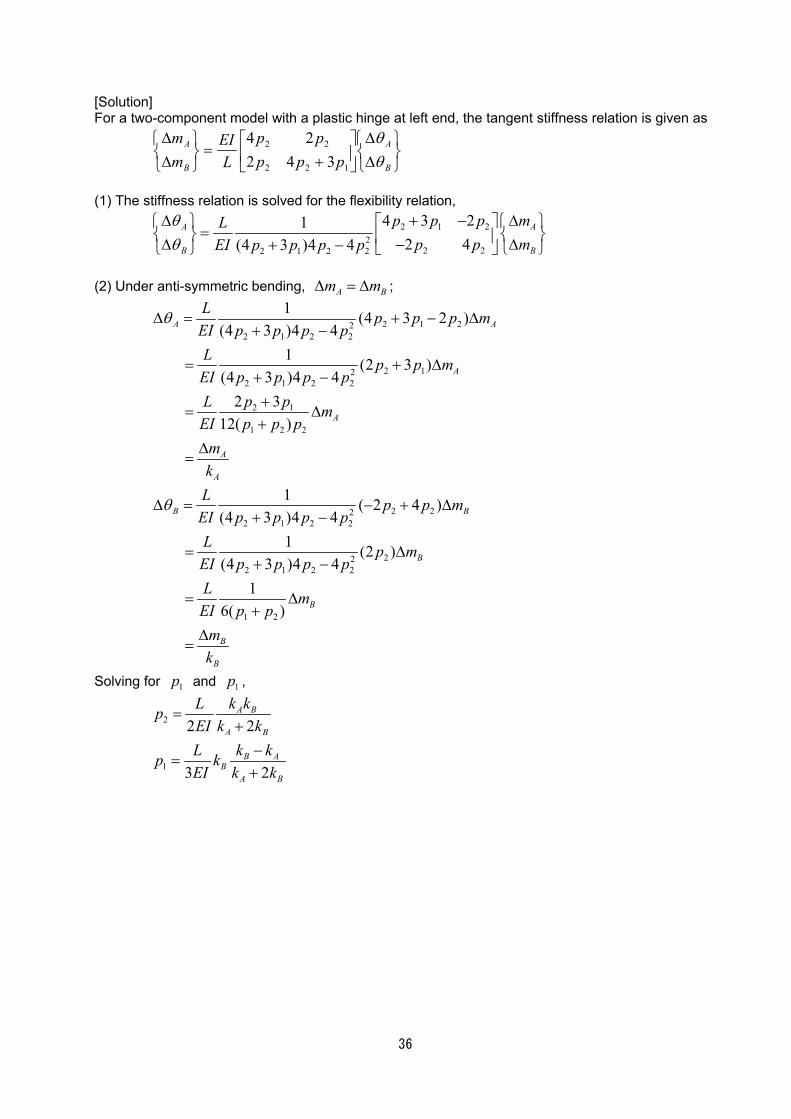
36

[Solution] For a two-component model with a plastic hinge at left end, the tangent stiffness relation is given as

∆∆

+

=

∆∆

B

A

B

A

ppppp

LEI

mm

θθ

122

22

34224

(1) The stiffness relation is solved for the flexibility relation,

2 1 22

2 22 1 2 2

4 3 212 4(4 3 )4 4

A A

B B

p p p mLp p mEI p p p p

θθ

∆ + − ∆ = ∆ − ∆+ −

(2) Under anti-symmetric bending, A Bm m∆ = ∆ ;

2 1 222 1 2 2

2 122 1 2 2

2 1

1 2 2

2 222 1 2 2

222 1 2 2

1 2

1 (4 3 2 )(4 3 )4 4

1 (2 3 )(4 3 )4 4

2 312( )

1 ( 2 4 )(4 3 )4 4

1 (2 )(4 3 )4 4

16( )

A A

A

A

A

A

B B

B

B

B

B

L p p p mEI p p p pL p p mEI p p p pL p p mEI p p p

mkL p p mEI p p p pL p mEI p p p pL mEI p p

mk

θ

θ

∆ = + − ∆+ −

= + ∆+ −+

= ∆+

∆=

∆ = − + ∆+ −

= ∆+ −

= ∆+

∆=

Solving for 1p and 1p ,

2

1

2 2

3 2

A B

A B

B AB

A B

L k kpEI k kL k kp kEI k k

=+

−=

+

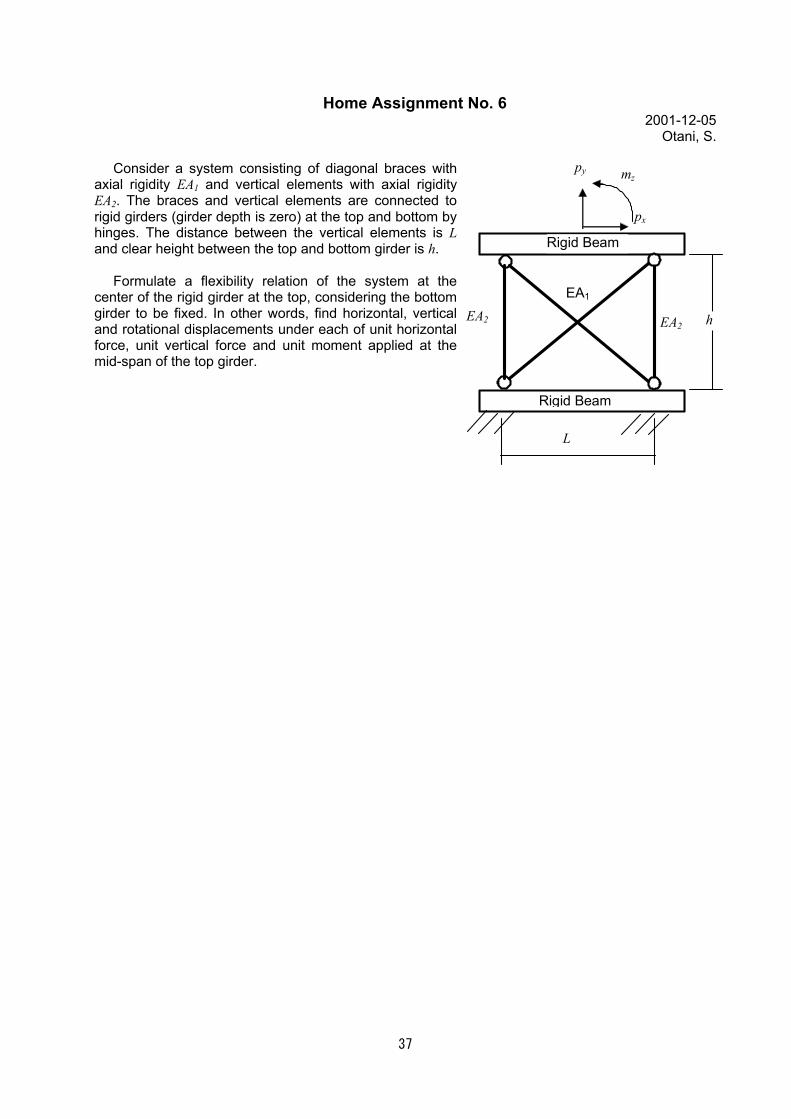
37

Home Assignment No. 6 2001-12-05

Otani, S.

Consider a system consisting of diagonal braces with axial rigidity EA1 and vertical elements with axial rigidity EA2. The braces and vertical elements are connected to rigid girders (girder depth is zero) at the top and bottom by hinges. The distance between the vertical elements is L and clear height between the top and bottom girder is h.

Formulate a flexibility relation of the system at the center of the rigid girder at the top, considering the bottom girder to be fixed. In other words, find horizontal, vertical and rotational displacements under each of unit horizontal force, unit vertical force and unit moment applied at the mid-span of the top girder.

h

Rigid Beam

Rigid Beam

L

px

py mz

EA1 EA2 EA2

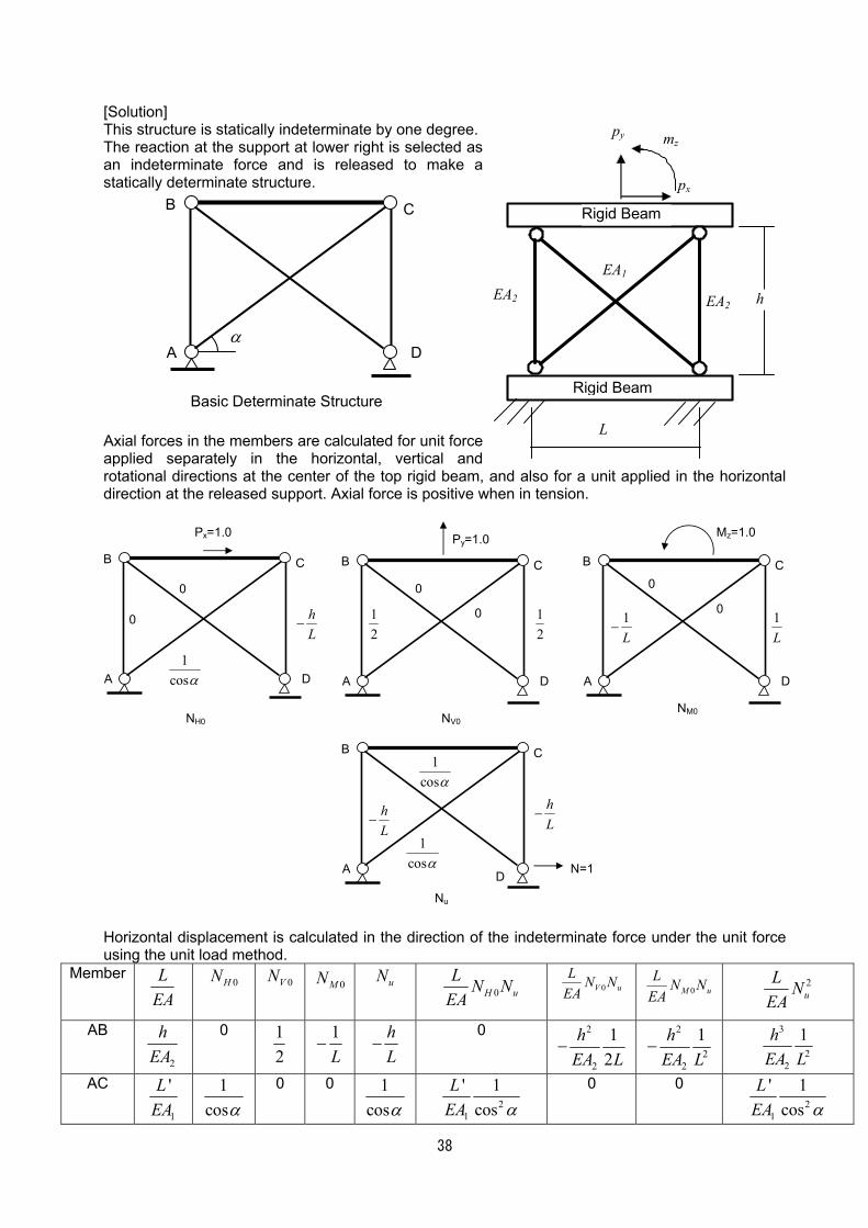
38

[Solution] This structure is statically indeterminate by one degree. The reaction at the support at lower right is selected as an indeterminate force and is released to make a statically determinate structure.

A

B C

D

Basic Determinate Structure

α

Axial forces in the members are calculated for unit force applied separately in the horizontal, vertical and rotational directions at the center of the top rigid beam, and also for a unit applied in the horizontal direction at the released support. Axial force is positive when in tension.

A

B C

D

hL

−

1cosα

hL

−

1cosα

N=1

A

B C

D A

B C

D

Py=1.0 Mz=1.0

12

12

A

B C

D

Px=1.0

hL

−

1cosα

0

0 0

0 1L

− 1L

0

0

NH0 NV0NM0

Nu

Horizontal displacement is calculated in the direction of the indeterminate force under the unit force using the unit load method.

Member LEA

0HN 0VN 0MN

uN 0H u

L N NEA

0V uL N N

EA

0M uL N N

EA

2u

L NEA

AB

2

hEA

0 1

2

1L

− hL

− 0 2

2

12

hEA L

− 2

22

1hEA L

− 3

22

1hEA L

AC

1

'LEA

1

cosα

0 0 1cosα 2

1

' 1cos

LEA α

0 0

21

' 1cos

LEA α

h

Rigid Beam

Rigid Beam

L

px

py mz

EA1 EA2 EA2

39

BD

1

'LEA

0 0 0 1

cosα0 0 0

21

' 1cos

LEA α

CD

2

hEA

hL

− 12

1L

hL

− 3

22

1hEA L

2

2

12

hEA L

− 2

22

1hEA L

3

22

1hEA L

Total - - - - - 3 3

21 2

1 '( )L hL EA EA

+2

2

1hEA L

− 0 3 3

21 2

2 '( )L hL EA EA

+

where 2 2'L L h= + From the displacement boundary condition at support D, the horizontal reaction 1N at the support due to unit horizontal load acting at the top beam is calculated;

3 3 3 3

12 21 2 1 2

1 ' 2 '( ) ( ) 0.0L h L hNL EA EA L EA EA

+ + + =

112

N = −

The horizontal reaction 1N due to unit vertical force is calculated;

2 3 3

122 1 2

2

21 3 3

1 2

1 2 '( ) 0.0

'2

h L h NEA L L EA EA

hL EAN

L hEA EA

− + + =

=+

The horizontal reaction 1N due to unit moment is calculated;

3 3

121 2

1

2 '0 ( ) 0.0

0.0

L h NL EA EA

N

+ + =

=

Therefore, the axial forces in he brace members due to unit load applied at the top beam are expressed as;

A

B C

D A

B C

D

Py=1.0 Mz=1.0

112

h NL

− 112

h NL

−

A

B C

D

Px=1.0

2hL

−

12cosα

2hL

12cosα

−

1

cosNα

1

cosNα

1L

− 1L

0

0

NH NVNM

0.00.5 2

21 3 3

1 2

'2

hL EAN

L hEA EA

=+

Calculation of displacement due to unit force applied at the center of top beam. Note that a unit force in the direction of desired displacement may be applied to the original structure, but unit forces in the direction of applied forces can be applied to the statically determinate structure.

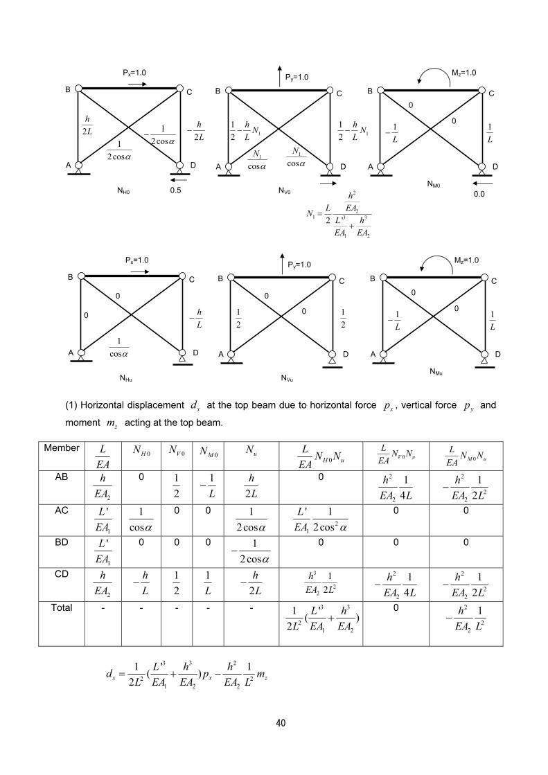
40

A

B C

D A

B C

D

Py=1.0 Mz=1.0

112

h NL

− 112

h NL

−

A

B C

D

Px=1.0

2hL

−

12cosα

2hL

12cosα

−

1

cosNα

1

cosNα

1L

− 1L

0

0

NH0 NV0NM0

0.00.5 2

21 3 3

1 2

'2

hL EAN

L hEA EA

=+

A

B C

D A

B C

D

Py=1.0 Mz=1.0

12

12

A

B C

D

Px=1.0

hL

−

1cosα

0

0 0

0 1L

− 1L

0

0

NHu NVuNMu

(1) Horizontal displacement xd at the top beam due to horizontal force xp , vertical force yp and

moment zm acting at the top beam.

Member LEA

0HN 0VN 0MN

uN 0H u

L N NEA

0V uL N N

EA

0M uL N N

EA

AB

2

hEA

0 1

2

1L

− 2hL

0 2

2

14

hEA L

2

22

12

hEA L

−

AC

1

'LEA

1

cosα

0 0 12cosα

21

' 12cos

LEA α

0 0

BD

1

'LEA

0 0 0 1

2cosα−

0 0 0

CD

2

hEA

hL

− 12

1L

2hL

− 3

22

12

hEA L

2

2

14

hEA L

− 2

22

12

hEA L

−

Total - - - - - 3 3

21 2

1 '( )2

L hL EA EA

+

0 2

22

1hEA L

−

3 3 2

2 21 2 2

1 ' 1( )2x x z

L h hd p mL EA EA EA L

= + −

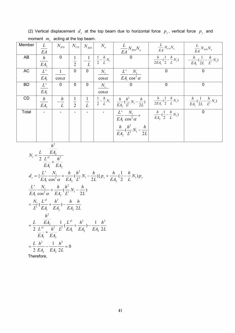
41

(2) Vertical displacement yd at the top beam due to horizontal force xp , vertical force yp and

moment zm acting at the top beam. Member L

EA 0HN 0VN

0MN

uN 0H u

L N NEA

0V uL N N

EA

0M uL N N

EA

AB

2

hEA

0 1

2

1L

− 112

h NL

− 0 1

2

1( )2 2

h h NEA L

− 12

2

1( )2

h h NEA L L

− −

AC

1

'LEA

1

cosα

0 0 1

cosNα

12

1

'cos

L NEA α

0 0

BD

1

'LEA

0 0 0 1

cosNα

0 0 0

CD

2

hEA

hL

− 12

1L

112

h NL

−2

122

( )2

h h hNEA L L

− 12

1( )2 2

h h NEA L

− 12

2

1( )2

h h NEA L L

−

Total - - - - - 12

12

122

'cos

( )2

L NEA

h h hNEA L L

α+

−

12

1( )2

h h NEA L

− 0

2

21 3 3

1 2

'2

hL EAN

L hEA EA

=+

21

1 12 21 2 2

' 1{ ( )} ( )cos 2 2y x y

L N h h h h hd N p N pEA EA L L EA Lα

= + − + −

21

12 21 2

3 312

1 2 22

3 3 22

3 3 21 2 2

1 22 2

2 2

' ( )cos 2

'( )2

1 ' 1( )'2 2

1 02 2

L N h h hNEA EA L L

N L h h hL EA EA EA L

hL L h hEA

L h L EA EA EA LEA EA

L h hEA EA L

α+ −

= + −

= + −+

= − =

Therefore,

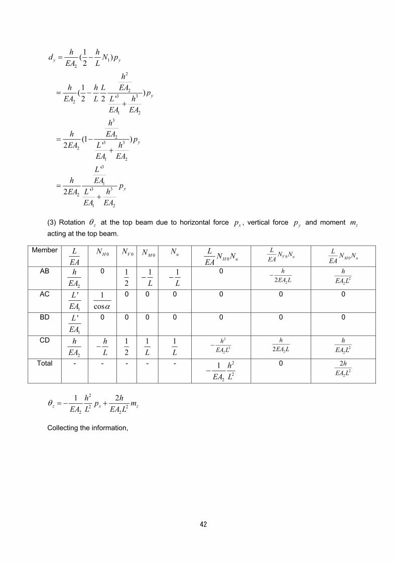
42

12

2

23 3

2

1 23

23 3

2

1 23

13 3

2

1 2

1( )2

1( )'2 2

(1 )'2

'

'2

y y

y

y

y

h hd N pEA L

hh h L EA p

L hEA LEA EA

hh EA p

L hEAEA EA

Lh EA p

L hEAEA EA

= −

= −+

= −+

=+

(3) Rotation zθ at the top beam due to horizontal force xp , vertical force yp and moment zm acting at the top beam.

Member LEA

0HN 0VN

0MN

uN 0H u

L N NEA

0V uL N N

EA

0M uL N N

EA

AB

2

hEA

0 1

2

1L

− 1L

− 0

22h

EA L−

22

hEA L

AC

1

'LEA

1

cosα

0 0 0 0 0 0

BD

1

'LEA

0 0 0 0 0 0 0

CD

2

hEA

hL

− 12

1L

1L

2

22

hEA L

− 22

hEA L

2

2

hEA L

Total - - - - - 2

22

1 hEA L

− 0

22

2hEA L

2

2 22 2

1 2z x z

h hp mEA L EA L

θ = − +

Collecting the information,

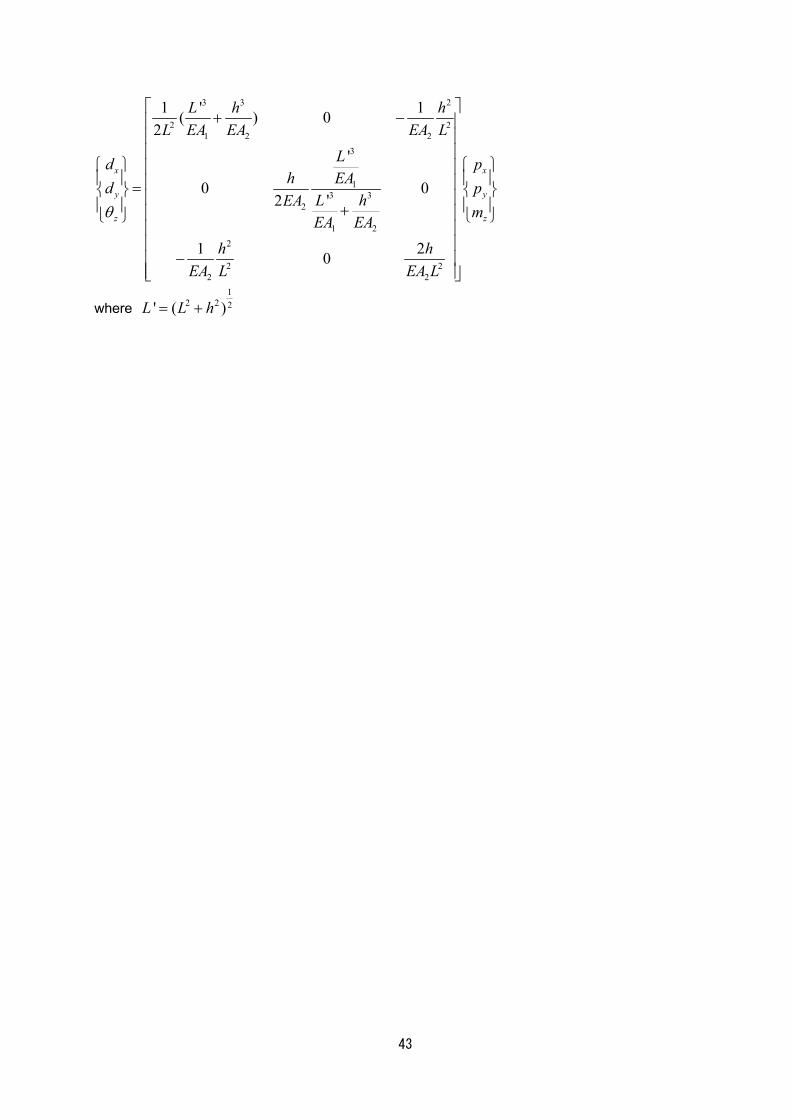
43

3 3 2

2 21 2 2

3

13 3

2

1 22

2 22 2

1 ' 1( ) 02

'

0 0'2

1 20

x x

y y

z z

L h hL EA EA EA L

Ld ph EAd p

L hEAmEA EA

h hEA L EA L

θ

+ −

= +

−

where 1

2 2 2' ( )L L h= +

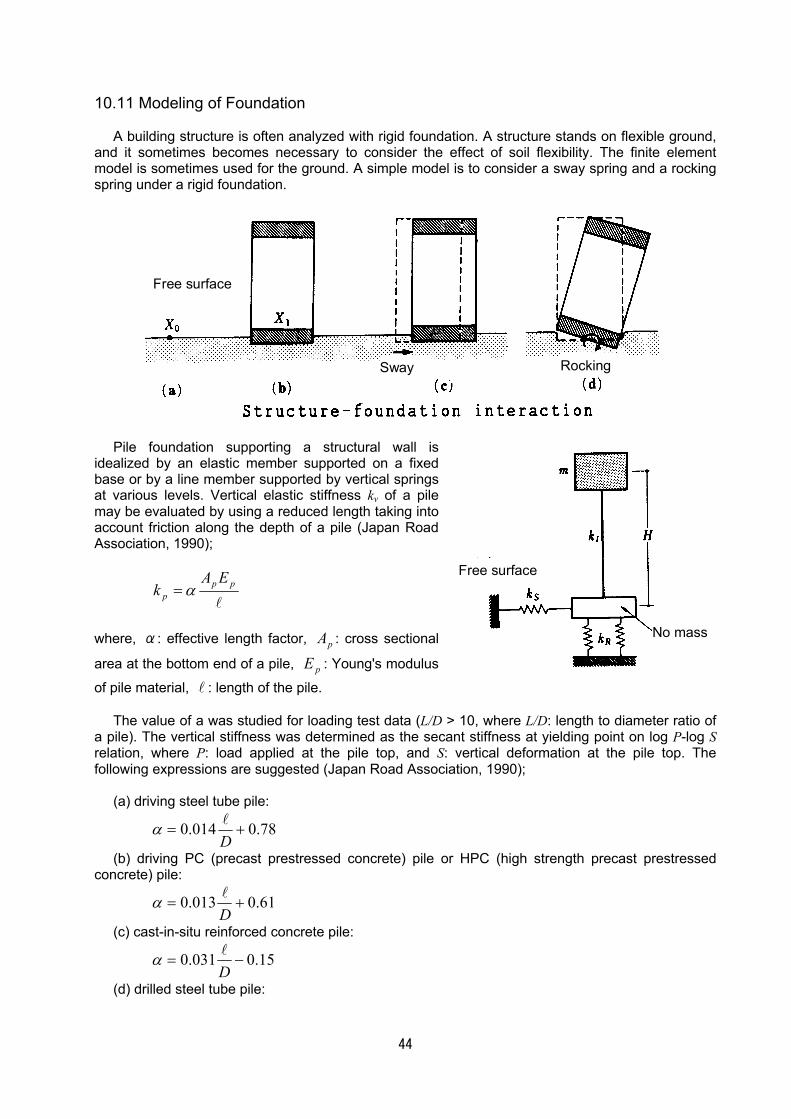
44

10.11 Modeling of Foundation

A building structure is often analyzed with rigid foundation. A structure stands on flexible ground, and it sometimes becomes necessary to consider the effect of soil flexibility. The finite element model is sometimes used for the ground. A simple model is to consider a sway spring and a rocking spring under a rigid foundation.

Free surface

Sway Rocking

Pile foundation supporting a structural wall is idealized by an elastic member supported on a fixed base or by a line member supported by vertical springs at various levels. Vertical elastic stiffness kv of a pile may be evaluated by using a reduced length taking into account friction along the depth of a pile (Japan Road Association, 1990);

l

ppp

EAk α=

where, α: effective length factor, pA : cross sectional

area at the bottom end of a pile, pE : Young's modulus

of pile material, l : length of the pile.

The value of a was studied for loading test data (L/D > 10, where L/D: length to diameter ratio of a pile). The vertical stiffness was determined as the secant stiffness at yielding point on log P-log S relation, where P: load applied at the pile top, and S: vertical deformation at the pile top. The following expressions are suggested (Japan Road Association, 1990);

(a) driving steel tube pile:

78.0014.0 +=Dlα

(b) driving PC (precast prestressed concrete) pile or HPC (high strength precast prestressed concrete) pile:

61.0013.0 +=Dlα

(c) cast-in-situ reinforced concrete pile:

15.0031.0 −=Dlα

(d) drilled steel tube pile:

Free surface

No mass

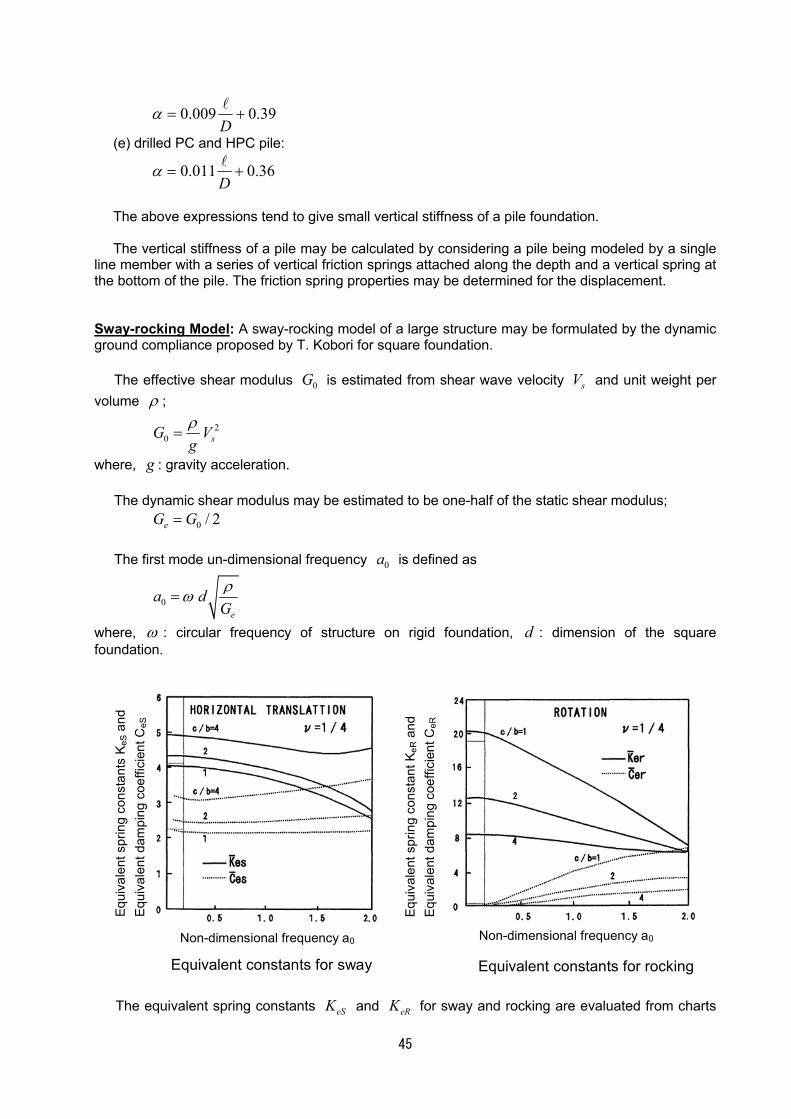
45

39.0009.0 +=Dlα

(e) drilled PC and HPC pile:

36.0011.0 +=Dlα

The above expressions tend to give small vertical stiffness of a pile foundation. The vertical stiffness of a pile may be calculated by considering a pile being modeled by a single

line member with a series of vertical friction springs attached along the depth and a vertical spring at the bottom of the pile. The friction spring properties may be determined for the displacement. Sway-rocking Model: A sway-rocking model of a large structure may be formulated by the dynamic ground compliance proposed by T. Kobori for square foundation.

The effective shear modulus 0G is estimated from shear wave velocity sV and unit weight per volume ρ ;

20 sG V

gρ

=

where, g : gravity acceleration.

The dynamic shear modulus may be estimated to be one-half of the static shear modulus; 0 / 2eG G=

The first mode un-dimensional frequency 0a is defined as

0e

a dGρω=

where, ω : circular frequency of structure on rigid foundation, d : dimension of the square foundation.

The equivalent spring constants eSK and eRK for sway and rocking are evaluated from charts

Equivalent constants for rockingEquivalent constants for sway

Non-dimensional frequency a0 Non-dimensional frequency a0

Equi

vale

nt s

prin

g co

nsta

nts

KeS

and

Eq

uiva

lent

dam

ping

coe

ffici

ent C

eS

Equi

vale

nt s

prin

g co

nsta

nt K

eR a

nd

Equi

vale

nt d

ampi

ng c

oeffi

cien

t CeR

46

for longitudinal dimension 2c and transverse dimension 2b. Spring constants SK and RK for

rocking and sway springs and associated damping factors Sh and Rh are evaluated as;

3

0

0

31212

S eS e

eR eR

eSS

eS

eRR

eR

K K d GGK K d

a ChK

a ChK

=

=

=

=

Reference:

Japan Road Association, "Standard Specifications for Design of Road Bridge and Commentary, Part

4: Underground Structures (in Japanese)," revised in February 1990.

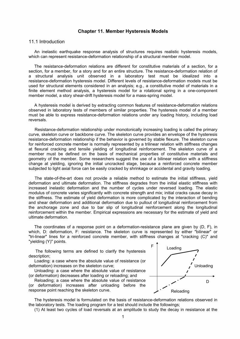
1

Chapter 11. Member Hysteresis Models 11.1 Introduction

An inelastic earthquake response analysis of structures requires realistic hysteresis models, which can represent resistance-deformation relationship of a structural member model.

The resistance-deformation relations are different for constitutive materials of a section, for a section, for a member, for a story and for an entire structure. The resistance-deformation relation of a structural analysis unit observed in a laboratory test must be idealized into a resistance-deformation hysteresis model. Different levels of resistance-deformation models must be used for structural elements considered in an analysis; e.g., a constitutive model of materials in a finite element method analysis, a hysteresis model for a rotational spring in a one-component member model, a story shear-drift hysteresis model for a mass-spring model.

A hysteresis model is derived by extracting common features of resistance-deformation relations observed in laboratory tests of members of similar properties. The hysteresis model of a member must be able to express resistance-deformation relations under any loading history, including load reversals.

Resistance-deformation relationship under monotonically increasing loading is called the primary curve, skeleton curve or backbone curve. The skeleton curve provides an envelope of the hysteresis resistance-deformation relationship if the behavior is governed by stable flexure. The skeleton curve for reinforced concrete member is normally represented by a trilinear relation with stiffness changes at flexural cracking and tensile yielding of longitudinal reinforcement. The skeleton curve of a member must be defined on the basis of mechanical properties of constitutive materials and geometry of the member. Some researchers suggest the use of a bilinear relation with a stiffness change at yielding, ignoring the initial uncracked stage, because a reinforced concrete member subjected to light axial force can be easily cracked by shrinkage or accidental and gravity loading.

The state-of-the-art does not provide a reliable method to estimate the initial stiffness, yield

deformation and ultimate deformation. The stiffness degrades from the initial elastic stiffness with increased inelastic deformation and the number of cycles under reversed loading. The elastic modulus of concrete varies significantly with concrete strength and mix; initial cracks cause decay in the stiffness. The estimate of yield deformation is more complicated by the interaction of bending and shear deformation and additional deformation due to pullout of longitudinal reinforcement from the anchorage zone and due to bar slip of longitudinal reinforcement along the longitudinal reinforcement within the member. Empirical expressions are necessary for the estimate of yield and ultimate deformation.

The coordinates of a response point on a deformation-resistance plane are given by (D, F), in which, D: deformation, F: resistance. The skeleton curve is represented by either "bilinear" or "tri-linear" lines for a reinforced concrete member, with stiffness changes at "cracking (C)" and "yielding (Y)" points.

The following terms are defined to clarify the hysteresis

description; Loading: a case where the absolute value of resistance (or

deformation) increases on the skeleton curve; Unloading: a case where the absolute value of resistance

(or deformation) decreases after loading or reloading; and Reloading; a case where the absolute value of resistance

(or deformation) increases after unloading before the response point reaching the skeleton curve.

The hysteresis model is formulated on the basis of resistance-deformation relations observed in

the laboratory tests. The loading program for a test should include the followings; (1) At least two cycles of load reversals at an amplitude to study the decay in resistance at the

Loading

Unloading

Reloading

D

F

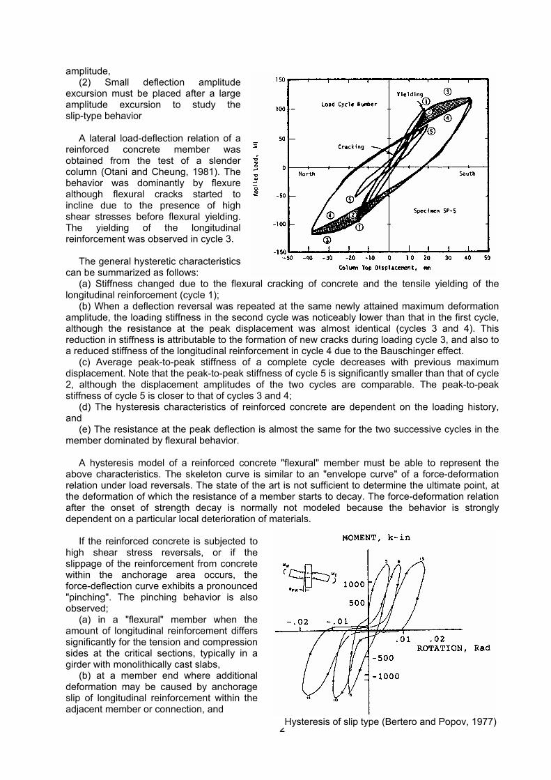
2

amplitude, (2) Small deflection amplitude

excursion must be placed after a large amplitude excursion to study the slip-type behavior

A lateral load-deflection relation of a reinforced concrete member was obtained from the test of a slender column (Otani and Cheung, 1981). The behavior was dominantly by flexure although flexural cracks started to incline due to the presence of high shear stresses before flexural yielding. The yielding of the longitudinal reinforcement was observed in cycle 3.

The general hysteretic characteristics

can be summarized as follows: (a) Stiffness changed due to the flexural cracking of concrete and the tensile yielding of the

longitudinal reinforcement (cycle 1); (b) When a deflection reversal was repeated at the same newly attained maximum deformation

amplitude, the loading stiffness in the second cycle was noticeably lower than that in the first cycle, although the resistance at the peak displacement was almost identical (cycles 3 and 4). This reduction in stiffness is attributable to the formation of new cracks during loading cycle 3, and also to a reduced stiffness of the longitudinal reinforcement in cycle 4 due to the Bauschinger effect.

(c) Average peak-to-peak stiffness of a complete cycle decreases with previous maximum displacement. Note that the peak-to-peak stiffness of cycle 5 is significantly smaller than that of cycle 2, although the displacement amplitudes of the two cycles are comparable. The peak-to-peak stiffness of cycle 5 is closer to that of cycles 3 and 4;

(d) The hysteresis characteristics of reinforced concrete are dependent on the loading history, and

(e) The resistance at the peak deflection is almost the same for the two successive cycles in the member dominated by flexural behavior.

A hysteresis model of a reinforced concrete "flexural" member must be able to represent the above characteristics. The skeleton curve is similar to an "envelope curve" of a force-deformation relation under load reversals. The state of the art is not sufficient to determine the ultimate point, at the deformation of which the resistance of a member starts to decay. The force-deformation relation after the onset of strength decay is normally not modeled because the behavior is strongly dependent on a particular local deterioration of materials.

If the reinforced concrete is subjected to high shear stress reversals, or if the slippage of the reinforcement from concrete within the anchorage area occurs, the force-deflection curve exhibits a pronounced "pinching". The pinching behavior is also observed;

(a) in a "flexural" member when the amount of longitudinal reinforcement differs significantly for the tension and compression sides at the critical sections, typically in a girder with monolithically cast slabs,

(b) at a member end where additional deformation may be caused by anchorage slip of longitudinal reinforcement within the adjacent member or connection, and

Hysteresis of slip type (Bertero and Popov, 1977)

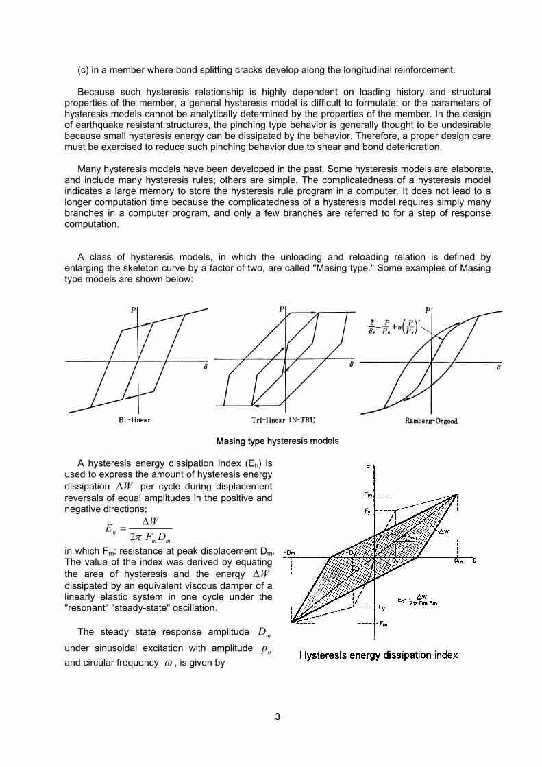
3

(c) in a member where bond splitting cracks develop along the longitudinal reinforcement.

Because such hysteresis relationship is highly dependent on loading history and structural properties of the member, a general hysteresis model is difficult to formulate; or the parameters of hysteresis models cannot be analytically determined by the properties of the member. In the design of earthquake resistant structures, the pinching type behavior is generally thought to be undesirable because small hysteresis energy can be dissipated by the behavior. Therefore, a proper design care must be exercised to reduce such pinching behavior due to shear and bond deterioration.

Many hysteresis models have been developed in the past. Some hysteresis models are elaborate, and include many hysteresis rules; others are simple. The complicatedness of a hysteresis model indicates a large memory to store the hysteresis rule program in a computer. It does not lead to a longer computation time because the complicatedness of a hysteresis model requires simply many branches in a computer program, and only a few branches are referred to for a step of response computation.

A class of hysteresis models, in which the unloading and reloading relation is defined by enlarging the skeleton curve by a factor of two, are called "Masing type." Some examples of Masing type models are shown below:

A hysteresis energy dissipation index (Eh) is

used to express the amount of hysteresis energy dissipation W∆ per cycle during displacement reversals of equal amplitudes in the positive and negative directions;

mm

h DFWE

π2∆

=

in which Fm: resistance at peak displacement Dm. The value of the index was derived by equating the area of hysteresis and the energy W∆ dissipated by an equivalent viscous damper of a linearly elastic system in one cycle under the "resonant" "steady-state" oscillation.

The steady state response amplitude mD

under sinusoidal excitation with amplitude op and circular frequency ω , is given by

Hysteresis energy dissipation index

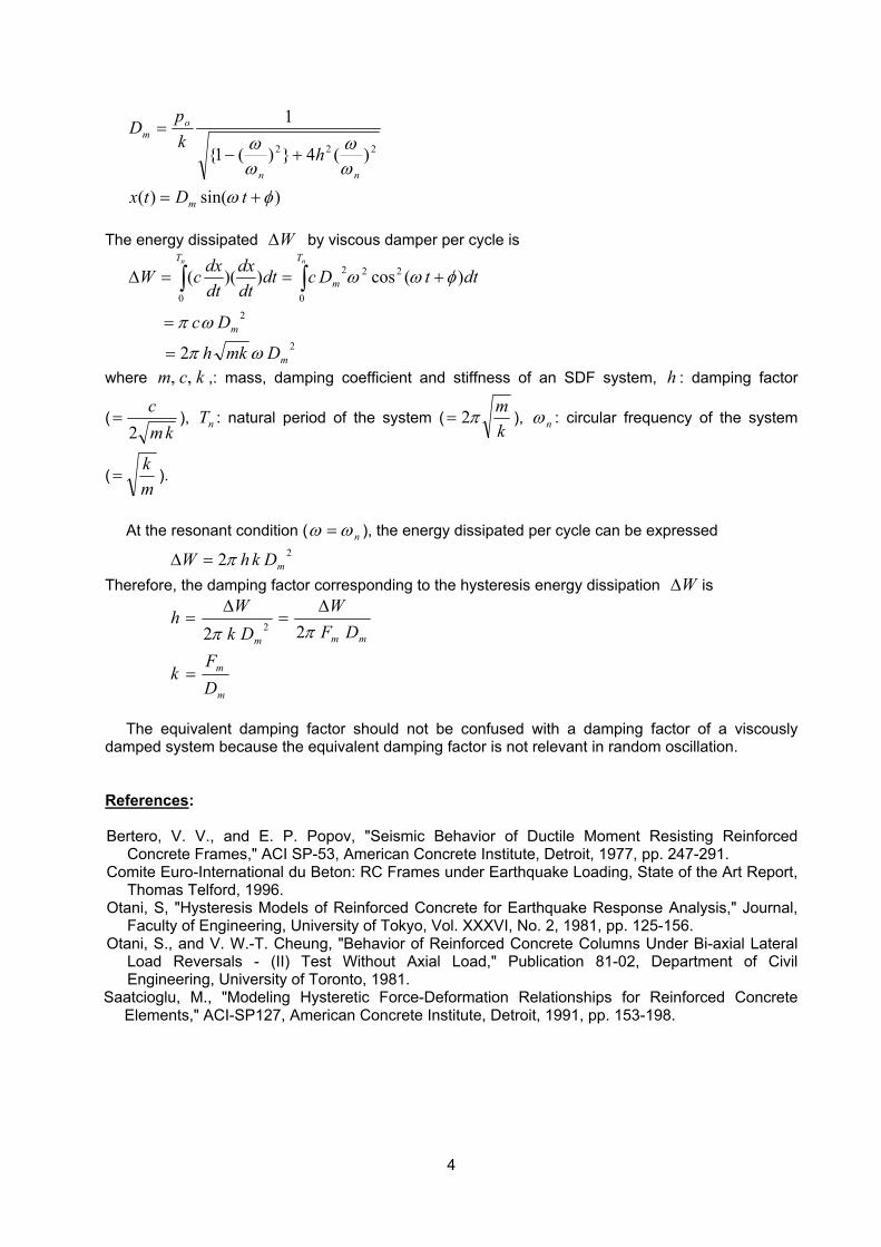
4

)sin()(

)(4})(1{

1

222

φωωω

ωω

+=

+−=

tDtx

hkp

D

m

nn

om

The energy dissipated W∆ by viscous damper per cycle is

2

2

22

0 0

2

2

)(cos))((

m

m

T T

m

Dmkh

Dc

dttDcdtdtdx

dtdxcW

n n

ωπ

ωπ

φωω

=

=

+==∆ ∫ ∫

where kcm ,, ,: mass, damping coefficient and stiffness of an SDF system, h : damping factor

(km

c2

= ), nT : natural period of the system (kmπ2= ), nω : circular frequency of the system

(mk

= ).

At the resonant condition ( nωω = ), the energy dissipated per cycle can be expressed

22 mDkhW π=∆ Therefore, the damping factor corresponding to the hysteresis energy dissipation W∆ is

m

m

mmm

DF

k

DFW

DkW

h

=

∆=

∆=

ππ 22 2

The equivalent damping factor should not be confused with a damping factor of a viscously

damped system because the equivalent damping factor is not relevant in random oscillation. References: Bertero, V. V., and E. P. Popov, "Seismic Behavior of Ductile Moment Resisting Reinforced

Concrete Frames," ACI SP-53, American Concrete Institute, Detroit, 1977, pp. 247-291. Comite Euro-International du Beton: RC Frames under Earthquake Loading, State of the Art Report,

Thomas Telford, 1996. Otani, S, "Hysteresis Models of Reinforced Concrete for Earthquake Response Analysis," Journal,

Faculty of Engineering, University of Tokyo, Vol. XXXVI, No. 2, 1981, pp. 125-156. Otani, S., and V. W.-T. Cheung, "Behavior of Reinforced Concrete Columns Under Bi-axial Lateral

Load Reversals - (II) Test Without Axial Load," Publication 81-02, Department of Civil Engineering, University of Toronto, 1981.

Saatcioglu, M., "Modeling Hysteretic Force-Deformation Relationships for Reinforced Concrete Elements," ACI-SP127, American Concrete Institute, Detroit, 1991, pp. 153-198.

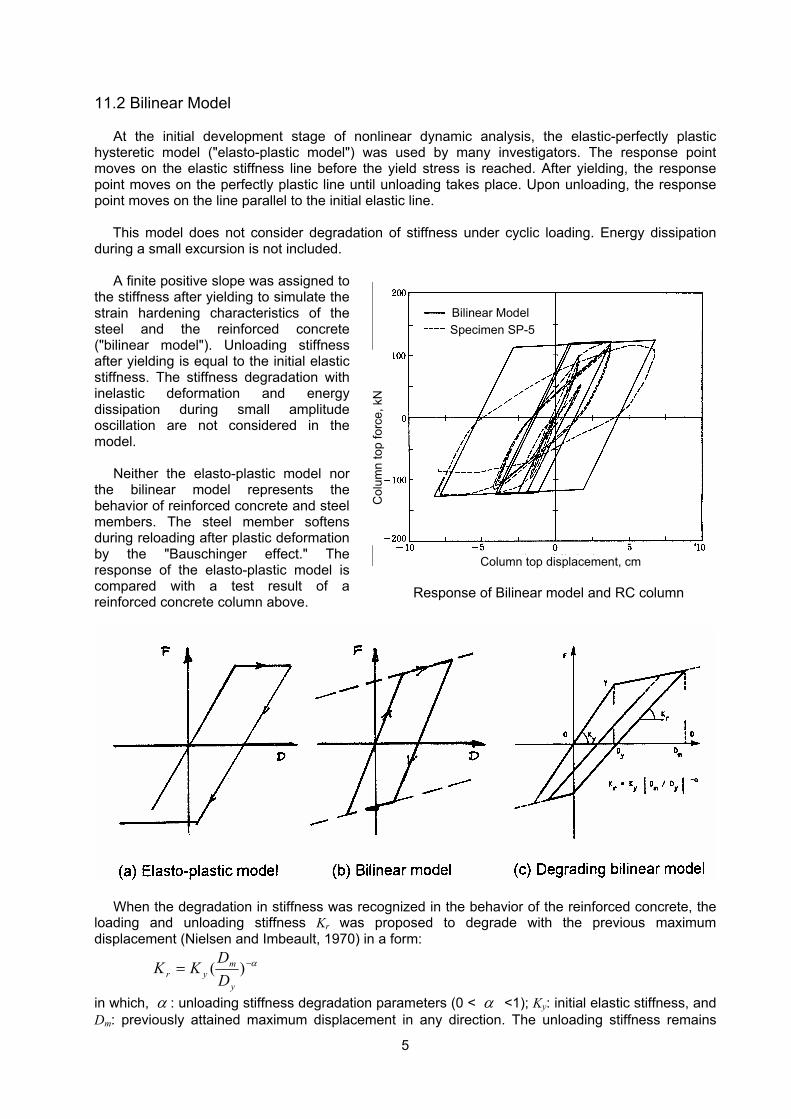
5

11.2 Bilinear Model

At the initial development stage of nonlinear dynamic analysis, the elastic-perfectly plastic hysteretic model ("elasto-plastic model") was used by many investigators. The response point moves on the elastic stiffness line before the yield stress is reached. After yielding, the response point moves on the perfectly plastic line until unloading takes place. Upon unloading, the response point moves on the line parallel to the initial elastic line.

This model does not consider degradation of stiffness under cyclic loading. Energy dissipation

during a small excursion is not included.

A finite positive slope was assigned to the stiffness after yielding to simulate the strain hardening characteristics of the steel and the reinforced concrete ("bilinear model"). Unloading stiffness after yielding is equal to the initial elastic stiffness. The stiffness degradation with inelastic deformation and energy dissipation during small amplitude oscillation are not considered in the model.

Neither the elasto-plastic model nor the bilinear model represents the behavior of reinforced concrete and steel members. The steel member softens during reloading after plastic deformation by the "Bauschinger effect." The response of the elasto-plastic model is compared with a test result of a reinforced concrete column above.

When the degradation in stiffness was recognized in the behavior of the reinforced concrete, the

loading and unloading stiffness Kr was proposed to degrade with the previous maximum displacement (Nielsen and Imbeault, 1970) in a form:

α−= )(y

myr D

DKK

in which, α : unloading stiffness degradation parameters (0 < α <1); Ky: initial elastic stiffness, and Dm: previously attained maximum displacement in any direction. The unloading stiffness remains

Bilinear ModelSpecimen SP-5

Column top displacement, cm

Col

umn

top

forc

e, k

N

Response of Bilinear model and RC column

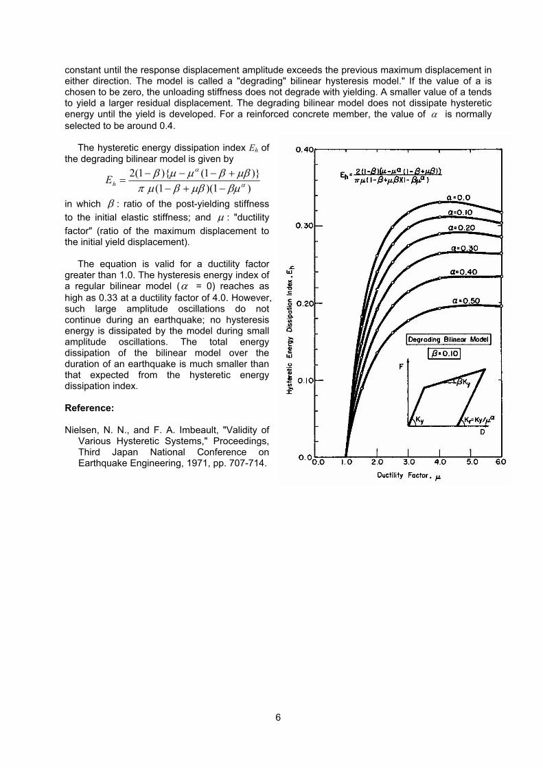
6

constant until the response displacement amplitude exceeds the previous maximum displacement in either direction. The model is called a "degrading" bilinear hysteresis model." If the value of a is chosen to be zero, the unloading stiffness does not degrade with yielding. A smaller value of a tends to yield a larger residual displacement. The degrading bilinear model does not dissipate hysteretic energy until the yield is developed. For a reinforced concrete member, the value of α is normally selected to be around 0.4.

The hysteretic energy dissipation index Eh of the degrading bilinear model is given by

)1)(1()}1(){1(2

α

α

βµµββµπµββµµβ

−+−+−−−

=hE

in which β : ratio of the post-yielding stiffness to the initial elastic stiffness; and µ : "ductility factor" (ratio of the maximum displacement to the initial yield displacement).

The equation is valid for a ductility factor greater than 1.0. The hysteresis energy index of a regular bilinear model (α = 0) reaches as high as 0.33 at a ductility factor of 4.0. However, such large amplitude oscillations do not continue during an earthquake; no hysteresis energy is dissipated by the model during small amplitude oscillations. The total energy dissipation of the bilinear model over the duration of an earthquake is much smaller than that expected from the hysteretic energy dissipation index. Reference: Nielsen, N. N., and F. A. Imbeault, "Validity of

Various Hysteretic Systems," Proceedings, Third Japan National Conference on Earthquake Engineering, 1971, pp. 707-714.

7

Appendix FORTRAN PROGRAM LISTING OF BILINEAR HYSTERESIS MODEL SUBROUTINE HYSTR1 (LL,SS,DD,DS,FF,FS) C C BILINEAR HYSTERESIS RULES FOR A GIVEN DISPLACEMENT INCREMENT. C C PROGRAMMED BY OTANI, S. C ON NOVEMBER 11,1978 C AT THE UNIVERSITY OF TORONTO. C C INPUT DATA C FY INITIAL YIELD FORCE LEVEL. C DY INITIAL YIELD DISPLACEMENT. C SY INITIAL ELASTIC STIFFNESS. C SU POST YIELDING STIFFNESS. C B0 STIFFNESS DEGRADATION FACTOR. C LL HYSTERESIS RULE POINTER AT PREVIOUS STEP. C DD DISPLACEMENT AT CURRENT STEP. C DS DISPLACEMENT AT PREVIOUS STEP. C C OUTPUT DATA C LL HYSTERESIS RULE POINTER AT CURRENT STEP. C SS STIFFNESS AT CURRENT STEP. C FF FORCE AT CURRENT STEP. C C VARIABLES C ES VARIABLE ELASTIC STIFFNESS AFTER FIRST YIELDING C DU UPPER LIMIT DISPLACEMENT FOR POST-YIELDING ELASTIC STAGE. C DL LOWER LIMIT DISPLACEMENT FOR POST-YIELDING ELASTIC STAGE. C FL LOWER LIMIT FORCE FOR POST-YIELDING ELASTIC STAGE. C DMX ABSOLUTE MAXIMUM DISPLACEMENT. C C C BILINEAR HYSTERESIS RULES C C RULE 1 INITIAL ELASTIC STAGE. C FF=SY*DD C RULE 2 POST-YIELDING STAGE IN POSITIVE DIRECTION. C FF= FY+(DD-DY)*SU C RULE 3 POST-YIELDING STAGE IN NEGATIVE DIRECTION. C FF=-FY+(DD+DY)*SU C RULE 4 POST-YIELDING ELASTIC STAGE. C FF=FL+(DD-DL)*SS C COMMON /STFF/MD,DC,DY,FC,FY,SC,SY,SU,B0,B1 GO TO (1,2,3,4),LL C INITIAL ELASTIC STAGE. 1 IF (DY-ABS(DD)) 110,110,100 100 FF=SY*DD GO TO 1000 110 DMX=DY IF (DD) 300,200,200 C POST-YIELDING STAGE IN POSITIVE DIRECTION. 2 IF (DD-DS) 220,220,210 200 LL=2 SS=SU 210 FF= FY+(DD-DY)*SU GO TO 1000 220 IF (DMX.LT.ABS(DS)) DMX=ABS(DS) ES=SY*(DY/DMX)**B0 DU=DS DL=(FS+FY-DY*SU-DU*ES)/(SU-ES) FL=-FY+(DL+DY)*SU IF (DD-DL) 300,300,400 C POST-YIELDING STAGE IN NEGATIVE DIRECTION. 3 IF (DD-DS) 310,320,320 300 LL=3 SS=SU

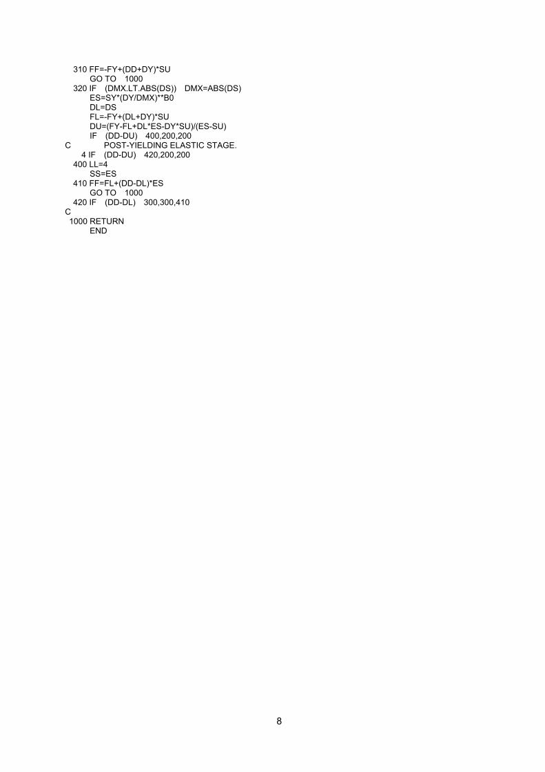
8

310 FF=-FY+(DD+DY)*SU GO TO 1000 320 IF (DMX.LT.ABS(DS)) DMX=ABS(DS) ES=SY*(DY/DMX)**B0 DL=DS FL=-FY+(DL+DY)*SU DU=(FY-FL+DL*ES-DY*SU)/(ES-SU) IF (DD-DU) 400,200,200 C POST-YIELDING ELASTIC STAGE. 4 IF (DD-DU) 420,200,200 400 LL=4 SS=ES 410 FF=FL+(DD-DL)*ES GO TO 1000 420 IF (DD-DL) 300,300,410 C 1000 RETURN END

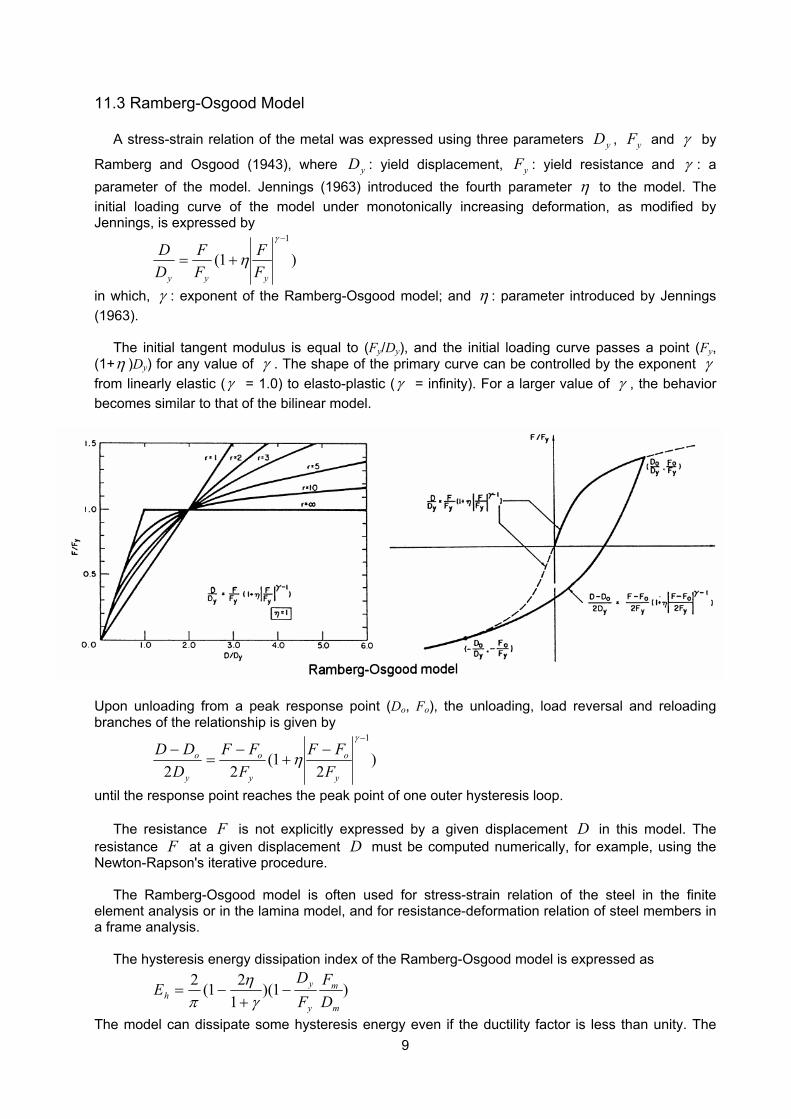
9

11.3 Ramberg-Osgood Model

A stress-strain relation of the metal was expressed using three parameters yD , yF and γ by

Ramberg and Osgood (1943), where yD : yield displacement, yF : yield resistance and γ : a parameter of the model. Jennings (1963) introduced the fourth parameter η to the model. The initial loading curve of the model under monotonically increasing deformation, as modified by Jennings, is expressed by

)1(1−

+=γ

ηyyy F

FFF

DD

in which, γ : exponent of the Ramberg-Osgood model; and η : parameter introduced by Jennings (1963).

The initial tangent modulus is equal to (Fy/Dy), and the initial loading curve passes a point (Fy, (1+η )Dy) for any value of γ . The shape of the primary curve can be controlled by the exponent γ from linearly elastic (γ = 1.0) to elasto-plastic (γ = infinity). For a larger value of γ , the behavior becomes similar to that of the bilinear model.

Upon unloading from a peak response point (Do, Fo), the unloading, load reversal and reloading branches of the relationship is given by

)2

1(22

1−−

+−

=−

γ

ηy

o

y

o

y

o

FFF

FFF

DDD

until the response point reaches the peak point of one outer hysteresis loop.

The resistance F is not explicitly expressed by a given displacement D in this model. The resistance F at a given displacement D must be computed numerically, for example, using the Newton-Rapson's iterative procedure.

The Ramberg-Osgood model is often used for stress-strain relation of the steel in the finite element analysis or in the lamina model, and for resistance-deformation relation of steel members in a frame analysis.

The hysteresis energy dissipation index of the Ramberg-Osgood model is expressed as

)1)(121(2

m

m

y

yh D

FFD

E −+

−=γη

π

The model can dissipate some hysteresis energy even if the ductility factor is less than unity. The

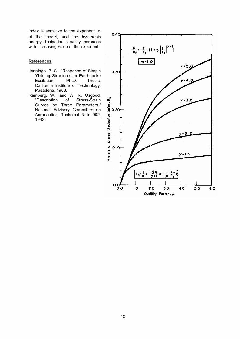
10

index is sensitive to the exponent γ of the model, and the hysteresis energy dissipation capacity increases with increasing value of the exponent. References: Jennings, P. C., "Response of Simple

Yielding Structures to Earthquake Excitation," Ph.D. Thesis, California Institute of Technology, Pasadena, 1963.

Ramberg, W., and W. R. Osgood, "Description of Stress-Strain Curves by Three Parameters," National Advisory Committee on Aeronautics, Technical Note 902, 1943.

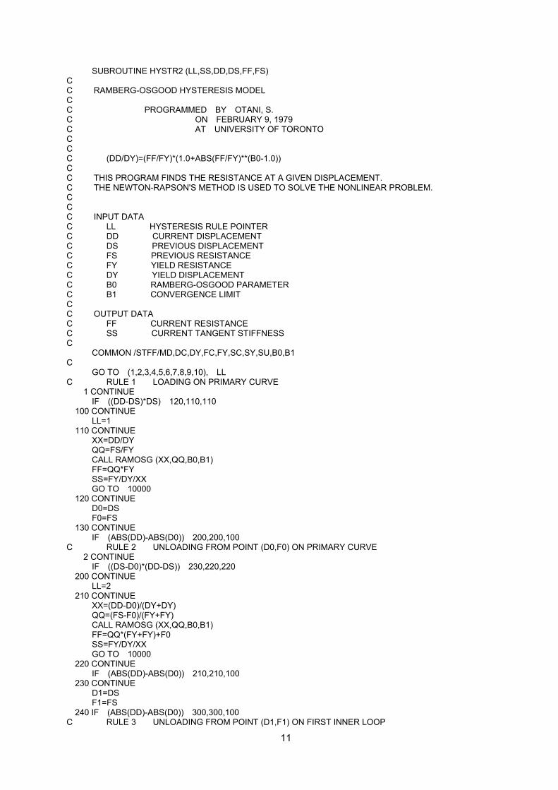
11

SUBROUTINE HYSTR2 (LL,SS,DD,DS,FF,FS) C C RAMBERG-OSGOOD HYSTERESIS MODEL C C PROGRAMMED BY OTANI, S. C ON FEBRUARY 9, 1979 C AT UNIVERSITY OF TORONTO C C C (DD/DY)=(FF/FY)*(1.0+ABS(FF/FY)**(B0-1.0)) C C THIS PROGRAM FINDS THE RESISTANCE AT A GIVEN DISPLACEMENT. C THE NEWTON-RAPSON'S METHOD IS USED TO SOLVE THE NONLINEAR PROBLEM. C C C INPUT DATA C LL HYSTERESIS RULE POINTER C DD CURRENT DISPLACEMENT C DS PREVIOUS DISPLACEMENT C FS PREVIOUS RESISTANCE C FY YIELD RESISTANCE C DY YIELD DISPLACEMENT C B0 RAMBERG-OSGOOD PARAMETER C B1 CONVERGENCE LIMIT C C OUTPUT DATA C FF CURRENT RESISTANCE C SS CURRENT TANGENT STIFFNESS C COMMON /STFF/MD,DC,DY,FC,FY,SC,SY,SU,B0,B1 C GO TO (1,2,3,4,5,6,7,8,9,10), LL C RULE 1 LOADING ON PRIMARY CURVE 1 CONTINUE IF ((DD-DS)*DS) 120,110,110 100 CONTINUE LL=1 110 CONTINUE XX=DD/DY QQ=FS/FY CALL RAMOSG (XX,QQ,B0,B1) FF=QQ*FY SS=FY/DY/XX GO TO 10000 120 CONTINUE D0=DS F0=FS 130 CONTINUE IF (ABS(DD)-ABS(D0)) 200,200,100 C RULE 2 UNLOADING FROM POINT (D0,F0) ON PRIMARY CURVE 2 CONTINUE IF ((DS-D0)*(DD-DS)) 230,220,220 200 CONTINUE LL=2 210 CONTINUE XX=(DD-D0)/(DY+DY) QQ=(FS-F0)/(FY+FY) CALL RAMOSG (XX,QQ,B0,B1) FF=QQ*(FY+FY)+F0 SS=FY/DY/XX GO TO 10000 220 CONTINUE IF (ABS(DD)-ABS(D0)) 210,210,100 230 CONTINUE D1=DS F1=FS 240 IF (ABS(DD)-ABS(D0)) 300,300,100 C RULE 3 UNLOADING FROM POINT (D1,F1) ON FIRST INNER LOOP

12

3 CONTINUE IF ((DS-D1)*(DD-DS)) 330,320,320 300 CONTINUE LL=3 310 CONTINUE XX=(DD-D1)/(DY+DY) QQ=(FS-F1)/(FY+FY) CALL RAMOSG (XX,QQ,B0,B1) FF=QQ*(FY+FY)+F1 SS=FY/DY/XX GO TO 10000 320 CONTINUE IF (ABS(DD)-ABS(D0)) 310,310,100 330 CONTINUE D2=DS F2=FS 340 CONTINUE IF ((D1-D2)*(DD-D1)) 400,130,130 C RULE 4 UNLOADING FROM POINT (D2,F2) ON FIRST INNER LOOP 4 CONTINUE IF ((D1-D2)*(DD-DS)) 430,420,420 400 CONTINUE LL=4 410 CONTINUE XX=(DD-D2)/(DY+DY) QQ=(FS-F2)/(FY+FY) CALL RAMOSG (XX,QQ,B0,B1) FF=QQ*(FY+FY)+F2 SS=FY/DY/XX GO TO 10000 420 CONTINUE IF ((D1-D2)*(DD-D1)) 410,130,130 430 CONTINUE D3=DS F3=FS 440 CONTINUE IF ((D1-D2)*(DD-D2)) 240,240,500 C RULE 5 UNLOADING FROM POINT (D3,F3) ON SECOND INNER LOOP 5 CONTINUE IF ((D2-D3)*(DD-DS)) 530,520,520 500 CONTINUE LL=5 510 CONTINUE XX=(DD-D3)/(DY+DY) QQ=(FS-F3)/(FY+FY) CALL RAMOSG (XX,QQ,B0,B1) FF=QQ*(FY+FY)+F3 SS=FY/DY/XX GO TO 10000 520 CONTINUE IF ((D2-D3)*(DD-D2)) 510,240,240 530 CONTINUE D4=DS F4=FS 540 CONTINUE IF ((D2-D3)*(DD-D3)) 340,340,600 C RULE 6 UNLOADING FROM POINT (D4,F4) ON SECOND INNER LOOP 6 CONTINUE IF ((D3-D4)*(DD-DS)) 630,620,620 600 CONTINUE LL=6 610 CONTINUE XX=(DD-D4)/(DY+DY) QQ=(FS-F4)/(FY+FY) CALL RAMOSG (XX,QQ,B0,B1) FF=QQ*(FY+FY)+F4 SS=FY/DY/XX GO TO 10000

13

620 CONTINUE IF ((D3-D4)*(DD-D3)) 610,340,340 630 CONTINUE D5=DS F5=FS 640 CONTINUE IF ((D3-D4)*(DD-D4)) 440,440,700 C RULE 7 UNLOADING FROM POINT (D5,F5) ON THIRD INNER LOOP 7 CONTINUE IF ((D4-D5)*(DD-DS)) 730,720,720 700 CONTINUE LL=7 710 CONTINUE XX=(DD-D5)/(DY+DY) QQ=(FS-F5)/(FY+FY) CALL RAMOSG (XX,QQ,B0,B1) FF=QQ*(FY+FY)+F5 SS=FY/DY/XX GO TO 10000 720 CONTINUE IF ((D4-D5)*(DD-D4)) 710,440,440 730 CONTINUE D6=DS F6=FS 740 CONTINUE IF ((D4-D5)*(DD-D5)) 540,540,800 C RULE 8 UNLOADING FROM POINT (D6,F6) ON THIRD INNER LOOP 8 CONTINUE IF ((D5-D6)*(DD-DS)) 830,820,820 800 CONTINUE LL=8 810 CONTINUE XX=(DD-D6)/(DY+DY) QQ=(FS-F6)/(FY+FY) CALL RAMOSG (XX,QQ,B0,B1) FF=QQ*(FY+FY)+F6 SS=FY/DY/XX GO TO 10000 820 CONTINUE IF ((D5-D6)*(DD-D5)) 810,540,540 830 CONTINUE D7=DS F7=FS 840 CONTINUE IF ((D5-D6)*(DD-D6)) 640,640,900 C RULE 9 UNLOADING FROM POINT (D7,F7) ON FOURTH INNER LOOP 9 CONTINUE IF ((D6-D7)*(DD-DS)) 930,920,920 900 CONTINUE LL=9 910 CONTINUE XX=(DD-D7)/(DY+DY) QQ=(FS-F7)/(FY+FY) CALL RAMOSG (XX,QQ,B0,B1) FF=QQ*(FY+FY)+F7 SS=FY/DY/XX GO TO 10000 920 CONTINUE IF ((D6-D7)*(DD-D6)) 910,640,640 930 CONTINUE D8=DS F8=FS 940 CONTINUE IF ((D6-D7)*(DD-D7)) 740,740,1000 C RULE 10 LINEAR RELATION BETWEEN POINTS (D7,F7) AND (D8,F8) 10 CONTINUE IF ((D7-D8)*(DD-D8)) 840,1020,1020 1000 CONTINUE

14

LL=10 1010 CONTINUE SS=(F7-F8)/(D7-D8) FF=F8+(DD-D8)*SS GO TO 10000 1020 CONTINUE IF ((D7-D8)*(DD-D7)) 1010,740,740 C 10000 CONTINUE RETURN END SUBROUTINE RAMOSG (XX,QQ,B0,ERR) C C DETERMINATION OF FORCE LEVEL QQ AT A GIVEN DISPLACEMENT XX OF A C RAMBERG-OSGOOD HYSTERESIS MODEL BY THE NEWTON-RAPSON'S ITERATIVE C PROCEDURE. C C XX=QQ*(1.0+ABS(QQ)**(B0-1.0)) C C C INPUT DATA C XX CURRENT DISPLACEMENT C QQ INITIAL VALUE OF RESISTANCE C B0 RAMBERG-OSGOOD PARAMETER C ERR CONVERGENCE LIMIT C C OUTPUT C QQ CURRENT RESISTANCE OF THE HYSTERESIS MODEL C XX CURRENT STIFFNESS C =1.0+B0*ABS(QQ)**(B0-1.0) C 10 CONTINUE Q0=QQ EX=ABS(Q0)**(B0-1.0) GQ=Q0*(1.0+EX)-XX TQ=1.0+B0*EX QQ=Q0-GQ/TQ IF (ABS(QQ-Q0)/(ABS(Q0)+ABS(QQ)).LT.ERR) GO TO 20 GO TO 10 20 CONTINUE XX=1.0+B0*ABS(QQ)**(B0-1.0) RETURN END

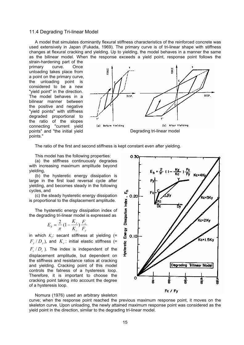
15

11.4 Degrading Tri-linear Model

A model that simulates dominantly flexural stiffness characteristics of the reinforced concrete was used extensively in Japan (Fukada, 1969). The primary curve is of tri-linear shape with stiffness changes at flexural cracking and yielding. Up to yielding, the model behaves in a manner the same as the bilinear model. When the response exceeds a yield point, response point follows the strain-hardening part of the primary curve. Once unloading takes place from a point on the primary curve, the unloading point is considered to be a new "yield point" in the direction. The model behaves in a bilinear manner between the positive and negative "yield points" with stiffness degraded proportional to the ratio of the slopes connecting "current yield points" and "the initial yield points."

The ratio of the first and second stiffness is kept constant even after yielding.

This model has the following properties: (a) the stiffness continuously degrades

with increasing maximum amplitude beyond yielding,

(b) the hysteretic energy dissipation is large in the first load reversal cycle after yielding, and becomes steady in the following cycles, and

(c) the steady hysteretic energy dissipation is proportional to the displacement amplitude.

The hysteretic energy dissipation index of the degrading tri-linear model is expressed as

y

c

c

yh F

FKK

E )1(2−=

π

in which Ky: secant stiffness at yielding (= yy DF / ), and cK : initial elastic stiffness (=

cc DF / ). The index is independent of the displacement amplitude, but dependent on the stiffness and resistance ratios at cracking and yielding. Cracking point of this model controls the fatness of a hysteresis loop. Therefore, it is important to choose the cracking point taking into account the degree of a hysteresis loop.

Nomura (1976) used an arbitrary skeleton curve; when the response point reached the previous maximum response point, it moves on the skeleton curve. Upon unloading, the newly attained maximum response point was considered as the yield point in the direction, similar to the degrading tri-linear model.

Degrading tri-linear model

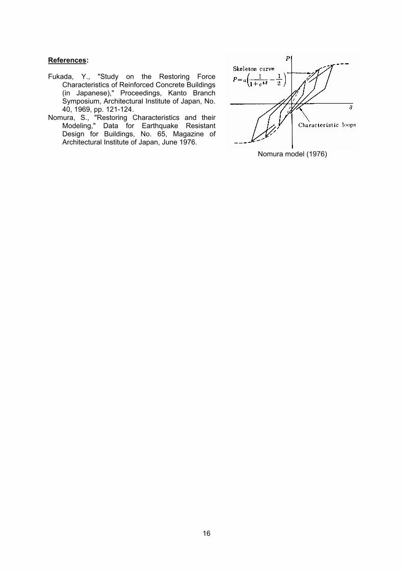
16

References: Fukada, Y., "Study on the Restoring Force

Characteristics of Reinforced Concrete Buildings (in Japanese)," Proceedings, Kanto Branch Symposium, Architectural Institute of Japan, No. 40, 1969, pp. 121-124.

Nomura, S., "Restoring Characteristics and their Modeling," Data for Earthquake Resistant Design for Buildings, No. 65, Magazine of Architectural Institute of Japan, June 1976.

Nomura model (1976)

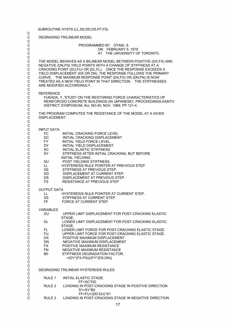
17

SUBROUTINE HYST6 (LL,SS,DD,DS,FF,FS) C C DEGRADING TRILINEAR MODEL C C PROGRAMMED BY OTANI, S. C ON FEBRUARY 9, 1979 C AT THE UNIVERSITY OF TORONTO. C C THE MODEL BEHAVES AS A BILINEAR MODEL BETWEEN POSITIVE (DX,FX) AND C NEGATIVE (DN,FN) YIELD POINTS WITH A CHANGE OF STIFFNESS AT A C CRACKING POINT (DU,FU) OR (DL,FL). ONCE THE RESPONSE EXCEEDS A C YIELD DISPLACEMENT (DX OR DN), THE RESPONSE FOLLOWS THE PRIMARY C CURVE. THE MAXIMUM RESPONSE POINT (DX,FX) OR (DN,FN) IS NOW C TREATED AS A NEW YIELD POINT IN THAT DIRECTION. THE STIFFNESSES C ARE MODIFIED ACCORDINGLY. C C REFERENCE C FUKADA, Y.,'STUDY ON THE RESTORING FORCE CHARACTERISTICS OF C REINFORCED CONCRETE BUILDINGS (IN JAPANESE)', PROCEEDINGS,KANTO C DISTRICT SYMPOSIUM, AIJ, NO.40, NOV. 1969, PP.121-4. C C THE PROGRAM COMPUTES THE RESISTANCE OF THE MODEL AT A GIVEN C DISPLACEMENT. C C C INPUT DATA C FC INITIAL CRACKING FORCE LEVEL C DC INITIAL CRACKING DISPLACEMENT C FY INITIAL YIELD FORCE LEVEL. C DY INITIAL YIELD DISPLACEMENT. C SC INITIAL ELASTIC STIFFNESS C SY STIFFNESS AFTER INITIAL CRACKING, BUT BEFORE C INITIAL YIELDING. C SU POST YIELDING STIFFNESS. C LL HYSTERESIS RULE POINTER AT PREVIOUS STEP. C SS STIFFNESS AT PREVIOUS STEP. C DD DISPLACEMENT AT CURRENT STEP. C DS DISPLACEMENT AT PREVIOUS STEP. C FS RESISTANCE AT PREVIOUS STEP C C OUTPUT DATA C LL HYSTERESIS RULE POINTER AT CURRENT STEP. C SS STIFFNESS AT CURRENT STEP. C FF FORCE AT CURRENT STEP. C C VARIABLES C DU UPPER LIMIT DISPLACEMENT FOR POST-CRACKING ELASTIC C STAGE. C DL LOWER LIMIT DISPLACEMENT FOR POST-CRACKING ELASTIC C STAGE. C FL LOWER LIMIT FORCE FOR POST-CRACKING ELASTIC STAGE. C FU UPPER LIMIT FORCE FOR POST-CRACKING ELASTIC STAGE. C DX POSITIVE MAXIMUM DISPLACEMENT C DN NEGATIVE MAXIMUM DISPLACEMENT C FX POSITIVE MAXIMUM RESISTANCE C FN NEGATIVE MAXIMUM RESISTANCE C B0 STIFFNESS DEGRADATION FACTOR. C =(DY*(FX-FN))/(FY*(DX-DN)) C C C DEGRADING TRILINEAR HYSTERESIS RULES C C RULE 1 INITIAL ELASTIC STAGE. C FF=SC*DD C RULE 2 LOADING IN POST-CRACKING STAGE IN POSITIVE DIRECTION C S1=SY*B0 C FF=FU+(DD-DU)*S1 C RULE 3 LOADING IN POST-CRACKING STAGE IN NEGATIVE DIRECTION

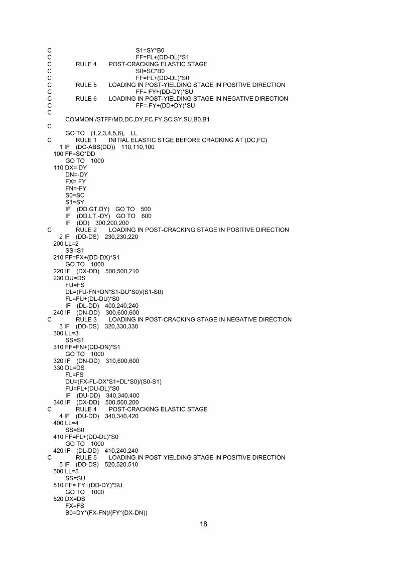
18

C S1=SY*B0 C FF=FL+(DD-DL)*S1 C RULE 4 POST-CRACKING ELASTIC STAGE C S0=SC*B0 C FF=FL+(DD-DL)*S0 C RULE 5 LOADING IN POST-YIELDING STAGE IN POSITIVE DIRECTION C FF= FY+(DD-DY)*SU C RULE 6 LOADING IN POST-YIELDING STAGE IN NEGATIVE DIRECTION C FF=-FY+(DD+DY)*SU C COMMON /STFF/MD,DC,DY,FC,FY,SC,SY,SU,B0,B1 C GO TO (1,2,3,4,5,6), LL C RULE 1 INITIAL ELASTIC STGE BEFORE CRACKING AT (DC,FC) 1 IF (DC-ABS(DD)) 110,110,100 100 FF=SC*DD GO TO 1000 110 DX= DY DN=-DY FX= FY FN=-FY S0=SC S1=SY IF (DD.GT.DY) GO TO 500 IF (DD.LT.-DY) GO TO 600 IF (DD) 300,200,200 C RULE 2 LOADING IN POST-CRACKING STAGE IN POSITIVE DIRECTION 2 IF (DD-DS) 230,230,220 200 LL=2 SS=S1 210 FF=FX+(DD-DX)*S1 GO TO 1000 220 IF (DX-DD) 500,500,210 230 DU=DS FU=FS DL=(FU-FN+DN*S1-DU*S0)/(S1-S0) FL=FU+(DL-DU)*S0 IF (DL-DD) 400,240,240 240 IF (DN-DD) 300,600,600 C RULE 3 LOADING IN POST-CRACKING STAGE IN NEGATIVE DIRECTION 3 IF (DD-DS) 320,330,330 300 LL=3 SS=S1 310 FF=FN+(DD-DN)*S1 GO TO 1000 320 IF (DN-DD) 310,600,600 330 DL=DS FL=FS DU=(FX-FL-DX*S1+DL*S0)/(S0-S1) FU=FL+(DU-DL)*S0 IF (DU-DD) 340,340,400 340 IF (DX-DD) 500,500,200 C RULE 4 POST-CRACKING ELASTIC STAGE 4 IF (DU-DD) 340,340,420 400 LL=4 SS=S0 410 FF=FL+(DD-DL)*S0 GO TO 1000 420 IF (DL-DD) 410,240,240 C RULE 5 LOADING IN POST-YIELDING STAGE IN POSITIVE DIRECTION 5 IF (DD-DS) 520,520,510 500 LL=5 SS=SU 510 FF= FY+(DD-DY)*SU GO TO 1000 520 DX=DS FX=FS B0=DY*(FX-FN)/(FY*(DX-DN))

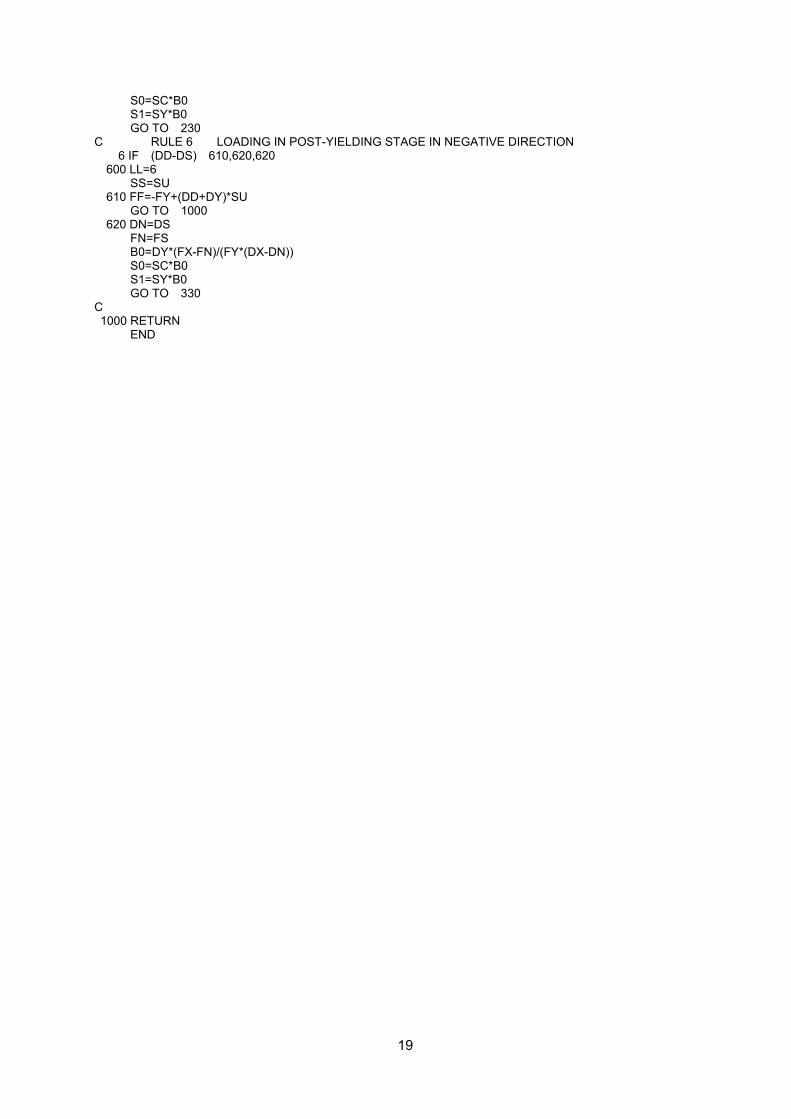
19

S0=SC*B0 S1=SY*B0 GO TO 230 C RULE 6 LOADING IN POST-YIELDING STAGE IN NEGATIVE DIRECTION 6 IF (DD-DS) 610,620,620 600 LL=6 SS=SU 610 FF=-FY+(DD+DY)*SU GO TO 1000 620 DN=DS FN=FS B0=DY*(FX-FN)/(FY*(DX-DN)) S0=SC*B0 S1=SY*B0 GO TO 330 C 1000 RETURN END

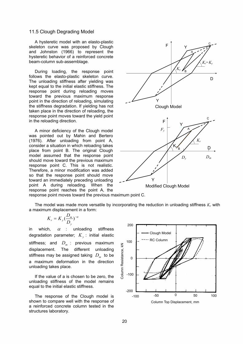
20

11.5 Clough Degrading Model

A hysteretic model with an elasto-plastic skeleton curve was proposed by Clough and Johnston (1966) to represent the hysteretic behavior of a reinforced concrete beam-column sub-assemblage.

During loading, the response point

follows the elasto-plastic skeleton curve. The unloading stiffness after yielding was kept equal to the initial elastic stiffness. The response point during reloading moves toward the previous maximum response point in the direction of reloading, simulating the stiffness degradation. If yielding has not taken place in the direction of reloading, the response point moves toward the yield point in the reloading direction.

A minor deficiency of the Clough model was pointed out by Mahin and Bertero (1976). After unloading from point A, consider a situation in which reloading takes place from point B. The original Clough model assumed that the response point should move toward the previous maximum response point C. This is not realistic. Therefore, a minor modification was added so that the response point should move toward an immediately preceding unloading point A during reloading. When the response point reaches the point A, the response point moves toward the previous maximum point C.

The model was made more versatile by incorporating the reduction in unloading stiffness Kr with a maximum displacement in a form:

α−= )(y

myr D

DKK

in which, α : unloading stiffness degradation parameter; yK : initial elastic

stiffness; and mD : previous maximum displacement. The different unloading stiffness may be assigned taking mD to be a maximum deformation in the direction unloading takes place.

If the value of a is chosen to be zero, the unloading stiffness of the model remains equal to the initial elastic stiffness.

The response of the Clough model is

shown to compare well with the response of a reinforced concrete column tested in the structures laboratory.

Clough Model

RC Column

Column Top Displacement, mm

Col

umn

Res

ista

nce,

kN

-100 -50 0 50 100

100

200

0

-100

-200

D

F

B

CY

Y

Kr=Ky Ky

A

Clough Model

D

F

B

C

Y

Y

Kr Ky

Dm Dy

Fy A

Modified Clough Model

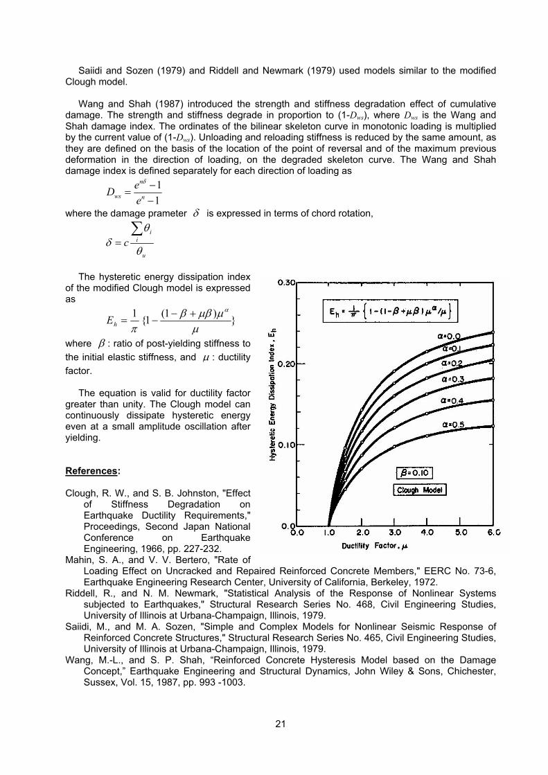
21

Saiidi and Sozen (1979) and Riddell and Newmark (1979) used models similar to the modified Clough model.

Wang and Shah (1987) introduced the strength and stiffness degradation effect of cumulative damage. The strength and stiffness degrade in proportion to (1-Dws), where Dws is the Wang and Shah damage index. The ordinates of the bilinear skeleton curve in monotonic loading is multiplied by the current value of (1-Dws). Unloading and reloading stiffness is reduced by the same amount, as they are defined on the basis of the location of the point of reversal and of the maximum previous deformation in the direction of loading, on the degraded skeleton curve. The Wang and Shah damage index is defined separately for each direction of loading as

11

n

ws n

eDe

δ −=

−

where the damage prameter δ is expressed in terms of chord rotation,

i

i

u

cθ

δθ

=∑

The hysteretic energy dissipation index

of the modified Clough model is expressed as

})1(1{1µ

µµββπ

α+−−=hE

where β : ratio of post-yielding stiffness to the initial elastic stiffness, and µ : ductility factor.

The equation is valid for ductility factor greater than unity. The Clough model can continuously dissipate hysteretic energy even at a small amplitude oscillation after yielding. References: Clough, R. W., and S. B. Johnston, "Effect

of Stiffness Degradation on Earthquake Ductility Requirements," Proceedings, Second Japan National Conference on Earthquake Engineering, 1966, pp. 227-232.

Mahin, S. A., and V. V. Bertero, "Rate of Loading Effect on Uncracked and Repaired Reinforced Concrete Members," EERC No. 73-6, Earthquake Engineering Research Center, University of California, Berkeley, 1972.

Riddell, R., and N. M. Newmark, "Statistical Analysis of the Response of Nonlinear Systems subjected to Earthquakes," Structural Research Series No. 468, Civil Engineering Studies, University of Illinois at Urbana-Champaign, Illinois, 1979.

Saiidi, M., and M. A. Sozen, "Simple and Complex Models for Nonlinear Seismic Response of Reinforced Concrete Structures," Structural Research Series No. 465, Civil Engineering Studies, University of Illinois at Urbana-Champaign, Illinois, 1979.

Wang, M.-L., and S. P. Shah, “Reinforced Concrete Hysteresis Model based on the Damage Concept,” Earthquake Engineering and Structural Dynamics, John Wiley & Sons, Chichester, Sussex, Vol. 15, 1987, pp. 993 -1003.

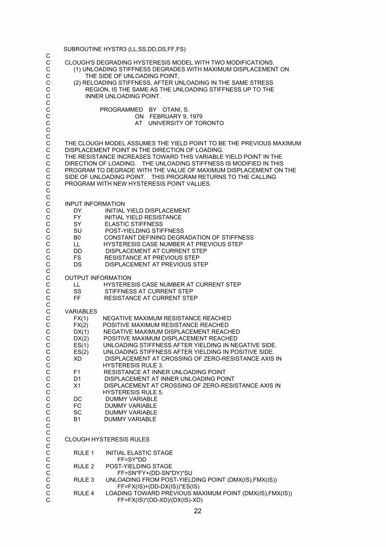
22

SUBROUTINE HYSTR3 (LL,SS,DD,DS,FF,FS) C C CLOUGH'S DEGRADING HYSTERESIS MODEL WITH TWO MODIFICATIONS. C (1) UNLOADING STIFFNESS DEGRADES WITH MAXIMUM DISPLACEMENT ON C THE SIDE OF UNLOADING POINT, C (2) RELOADING STIFFNESS, AFTER UNLOADING IN THE SAME STRESS C REGION, IS THE SAME AS THE UNLOADING STIFFNESS UP TO THE C INNER UNLOADING POINT. C C PROGRAMMED BY OTANI, S. C ON FEBRUARY 9, 1979 C AT UNIVERSITY OF TORONTO C C C THE CLOUGH MODEL ASSUMES THE YIELD POINT TO BE THE PREVIOUS MAXIMUM C DISPLACEMENT POINT IN THE DIRECTION OF LOADING. C THE RESISTANCE INCREASES TOWARD THIS VARIABLE YIELD POINT IN THE C DIRECTION OF LOADING. THE UNLOADING STIFFNESS IS MODIFIED IN THIS C PROGRAM TO DEGRADE WITH THE VALUE OF MAXIMUM DISPLACEMENT ON THE C SIDE OF UNLOADING POINT. THIS PROGRAM RETURNS TO THE CALLING C PROGRAM WITH NEW HYSTERESIS POINT VALUES. C C C INPUT INFORMATION C DY INITIAL YIELD DISPLACEMENT C FY INITIAL YIELD RESISTANCE C SY ELASTIC STIFFNESS C SU POST-YIELDING STIFFNESS C B0 CONSTANT DEFINING DEGRADATION OF STIFFNESS C LL HYSTERESIS CASE NUMBER AT PREVIOUS STEP C DD DISPLACEMENT AT CURRENT STEP C FS RESISTANCE AT PREVIOUS STEP C DS DISPLACEMENT AT PREVIOUS STEP C C OUTPUT INFORMATION C LL HYSTERESIS CASE NUMBER AT CURRENT STEP C SS STIFFNESS AT CURRENT STEP C FF RESISTANCE AT CURRENT STEP C C VARIABLES C FX(1) NEGATIVE MAXIMUM RESISTANCE REACHED C FX(2) POSITIVE MAXIMUM RESISTANCE REACHED C DX(1) NEGATIVE MAXIMUM DISPLACEMENT REACHED C DX(2) POSITIVE MAXIMUM DISPLACEMENT REACHED C ES(1) UNLOADING STIFFNESS AFTER YIELDING IN NEGATIVE SIDE. C ES(2) UNLOADING STIFFNESS AFTER YIELDING IN POSITIVE SIDE. C XD DISPLACEMENT AT CROSSING OF ZERO-RESISTANCE AXIS IN C HYSTERESIS RULE 3. C F1 RESISTANCE AT INNER UNLOADING POINT C D1 DISPLACEMENT AT INNER UNLOADING POINT C X1 DISPLACEMENT AT CROSSING OF ZERO-RESISTANCE AXIS IN C HYSTERESIS RULE 5. C DC DUMMY VARIABLE C FC DUMMY VARIABLE C SC DUMMY VARIABLE C B1 DUMMY VARIABLE C C C CLOUGH HYSTERESIS RULES C C RULE 1 INITIAL ELASTIC STAGE C FF=SY*DD C RULE 2 POST-YIELDING STAGE C FF=SN*FY+(DD-SN*DY)*SU C RULE 3 UNLOADING FROM POST-YIELDING POINT (DMX(IS),FMX(IS)) C FF=FX(IS)+(DD-DX(IS))*ES(IS) C RULE 4 LOADING TOWARD PREVIOUS MAXIMUM POINT (DMX(IS),FMX(IS)) C FF=FX(IS)*(DD-XD)/(DX(IS)-XD)

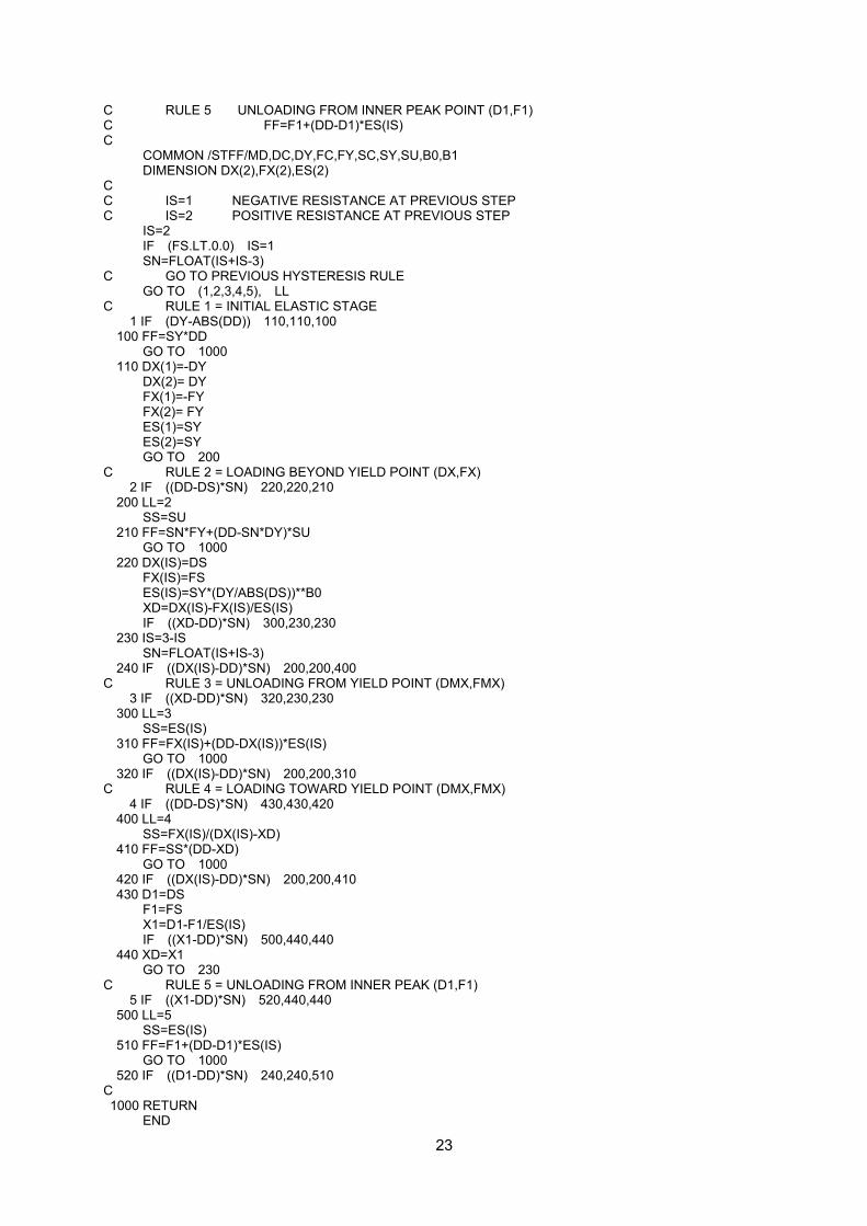
23

C RULE 5 UNLOADING FROM INNER PEAK POINT (D1,F1) C FF=F1+(DD-D1)*ES(IS) C COMMON /STFF/MD,DC,DY,FC,FY,SC,SY,SU,B0,B1 DIMENSION DX(2),FX(2),ES(2) C C IS=1 NEGATIVE RESISTANCE AT PREVIOUS STEP C IS=2 POSITIVE RESISTANCE AT PREVIOUS STEP IS=2 IF (FS.LT.0.0) IS=1 SN=FLOAT(IS+IS-3) C GO TO PREVIOUS HYSTERESIS RULE GO TO (1,2,3,4,5), LL C RULE 1 = INITIAL ELASTIC STAGE 1 IF (DY-ABS(DD)) 110,110,100 100 FF=SY*DD GO TO 1000 110 DX(1)=-DY DX(2)= DY FX(1)=-FY FX(2)= FY ES(1)=SY ES(2)=SY GO TO 200 C RULE 2 = LOADING BEYOND YIELD POINT (DX,FX) 2 IF ((DD-DS)*SN) 220,220,210 200 LL=2 SS=SU 210 FF=SN*FY+(DD-SN*DY)*SU GO TO 1000 220 DX(IS)=DS FX(IS)=FS ES(IS)=SY*(DY/ABS(DS))**B0 XD=DX(IS)-FX(IS)/ES(IS) IF ((XD-DD)*SN) 300,230,230 230 IS=3-IS SN=FLOAT(IS+IS-3) 240 IF ((DX(IS)-DD)*SN) 200,200,400 C RULE 3 = UNLOADING FROM YIELD POINT (DMX,FMX) 3 IF ((XD-DD)*SN) 320,230,230 300 LL=3 SS=ES(IS) 310 FF=FX(IS)+(DD-DX(IS))*ES(IS) GO TO 1000 320 IF ((DX(IS)-DD)*SN) 200,200,310 C RULE 4 = LOADING TOWARD YIELD POINT (DMX,FMX) 4 IF ((DD-DS)*SN) 430,430,420 400 LL=4 SS=FX(IS)/(DX(IS)-XD) 410 FF=SS*(DD-XD) GO TO 1000 420 IF ((DX(IS)-DD)*SN) 200,200,410 430 D1=DS F1=FS X1=D1-F1/ES(IS) IF ((X1-DD)*SN) 500,440,440 440 XD=X1 GO TO 230 C RULE 5 = UNLOADING FROM INNER PEAK (D1,F1) 5 IF ((X1-DD)*SN) 520,440,440 500 LL=5 SS=ES(IS) 510 FF=F1+(DD-D1)*ES(IS) GO TO 1000 520 IF ((D1-DD)*SN) 240,240,510 C 1000 RETURN END

24

11.6 Takeda Degrading Model

Based on the experimental observation on the behavior of a number of medium-size reinforced concrete members tested under lateral load reversals with light to medium amount of axial load, a hysteresis model was developed by Takeda, Sozen and Nielsen (1970). The model has been widely used in the nonlinear earthquake response analysis of reinforced concrete structures. Takeda Hysteresis Model:

1. Condition: The cracking load, Pcr, has not been exceeded in one direction. The load is reversed from a load P in the other direction. The load P is smaller than the yield load Py.

Rule: Unloading follows a straight line from the position at load P to the point representing the cracking load in the other direction.

2. Condition: A load P1 is reached in one direction on the primary curve such that P1 is larger than

Pcr but smaller the yield load Py. The load is then reversed to -P2 such that P2<P1. Rule: Unload parallel to loading curve for that half cycle. 3. Condition: A load P1 is reached in one direction such that P1 is larger than Pcr but not larger

than the yield load Py. The load is then reversed to -P3 such that P3>P1. Rule: Unloading follows a straight line joining the point of return and the point representing

cracking in the other direction. 4. Condition: One or more loading cycles have occurred. The load is zero. Rule: To construct the loading curve, connect the point at zero load to the point reached in the

previous cycle, if that point lies on the primary curve or on a line aimed at a point on the primary curve. If the previous loading cycle contains no such point, go to the preceding cycle and continue the process until such a point is found. Then connect that point to the point at zero load.

Exception: If the yield point has not been exceeded and if the point at zero load is not located within the horizontal projection of the primary curve for that direction of loading, connect the point at zero load to the yield point to obtain the loading slope.

5. Condition: The yield load Py is exceeded in one direction. Rule: Unloading curve follows the slope given by the following equation:

4.0)(DD

kk yyr =

in which rk : slope of unloading curve, yk : slope of a line joining the yield point in one direction to

the cracking point in the other direction, D : maximum deflection attained in the direction of the loading, and yD : deflection at yield.

6. Condition: The yield load is exceeded in one direction but the cracking load is not exceeded in

the opposite direction. Rule: Unloading follows Rule 5. Loading in the other direction continues as an extension of the

unloading line up to the cracking load. Then, the loading curve is aimed at the yield point. 7. Condition: One or more loading cycles have occurred. Rule: If the immediately preceding quarter-cycle remained on one side of the zero-load axis,

unload at the rate based on rule 2, 3 and 5 whichever governed in the previous loading history. If the immediately preceding quarter-cycle crossed the zero-load axis, unload at 70% of the rate based on rule 2, 3, or 5, whichever governed in the previous loading history, but not at a slope flatter than the immediately preceding loading slope.

Takeda model included (a) stiffness changes at flexural cracking and yielding, (b) hysteresis rules for inner hysteresis loops inside the outer loop, and (c) unloading stiffness degradation with deformation. The response point moves toward a peak of the one outer hysteresis loop. The unloading stiffness Kr after yielding is given by

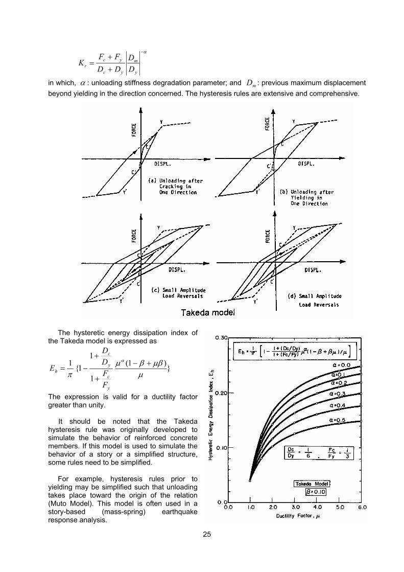
25

α−

++

=y

m

yc

ycr D

DDDFF

K

in which, α : unloading stiffness degradation parameter; and mD : previous maximum displacement beyond yielding in the direction concerned. The hysteresis rules are extensive and comprehensive.

The hysteretic energy dissipation index of

the Takeda model is expressed as

})1(

1

11{1

µµββµ

π

α +−

+

+−=

y

c

y

c

h

FFDD

E

The expression is valid for a ductility factor greater than unity.

It should be noted that the Takeda hysteresis rule was originally developed to simulate the behavior of reinforced concrete members. If this model is used to simulate the behavior of a story or a simplified structure, some rules need to be simplified.

For example, hysteresis rules prior to yielding may be simplified such that unloading takes place toward the origin of the relation (Muto Model). This model is often used in a story-based (mass-spring) earthquake response analysis.

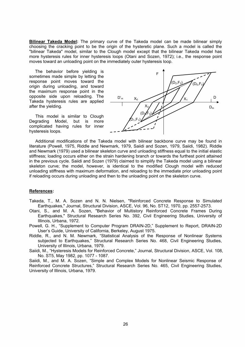
26

Bilinear Takeda Model: The primary curve of the Takeda model can be made bilinear simply choosing the cracking point to be the origin of the hysteretic plane. Such a model is called the "bilinear Takeda" model, similar to the Clough model except that the bilinear Takeda model has more hysteresis rules for inner hysteresis loops (Otani and Sozen, 1972); i.e., the response point moves toward an unloading point on the immediately outer hysteresis loop.

The behavior before yielding is sometimes made simple by letting the response point moves toward the origin during unloading, and toward the maximum response point in the opposite side upon reloading. The Takeda hysteresis rules are applied after the yielding.

This model is similar to Clough Degrading Model, but is more complicated having rules for inner hysteresis loops.

Additional modifications of the Takeda model with bilinear backbone curve may be found in literature (Powell, 1975, Riddle and Newmark, 1979, Saiidi and Sozen, 1979, Saiidi, 1982). Riddle and Newmark (1979) used a bilinear skeleton curve and unloading stiffness equal to the initial elastic stiffness; loading occurs either on the strain hardening branch or towards the furthest point attained in the previous cycle. Saiidi and Sozen (1979) claimed to simplify the Takeda model using a bilinear skeleton curve; the model, however, is identical to the modified Clough model with reduced unloading stiffness with maximum deformation, and reloading to the immediate prior unloading point if reloading occurs during unloading and then to the unloading point on the skeleton curve. References: Takeda, T., M. A. Sozen and N. N. Nielsen, "Reinforced Concrete Response to Simulated

Earthquakes," Journal, Structural Division, ASCE, Vol. 96, No. ST12, 1970, pp. 2557-2573. Otani, S., and M. A. Sozen, "Behavior of Multistory Reinforced Concrete Frames During

Earthquakes," Structural Research Series No. 392, Civil Engineering Studies, University of Illinois, Urbana, 1972.

Powell, G. H., “Supplement to Computer Program DRAIN-2D,” Supplement to Report, DRAIN-2D User’s Guide, University of California, Berkeley, August 1975.

Riddle, R., and N. M. Newmark, “Statistical Analysis of the Response of Nonlinear Systems subjected to Earthquakes,” Structural Research Series No. 468, Civil Engineering Studies, University of Illinois, Urbana, 1979.

Saiidi, M., “Hysteresis Models for Reinforced Concrete,” Journal, Structural Division, ASCE, Vol. 108, No. ST5, May 1982, pp. 1077 - 1087.

Saiidi, M., and M. A. Sozen, “Simple and Complex Models for Nonlinear Seismic Response of Reinforced Concrete Structures,” Structural Research Series No. 465, Civil Engineering Studies, University of Illinois, Urbana, 1979.

D

F

Dm

D’m X0

(D0,F0)

X1

(D1,F1)

X3

(D2,F2)

(D3,F3)

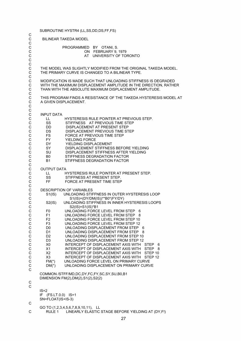
27

SUBROUTINE HYSTR4 (LL,SS,DD,DS,FF,FS) C C BILINEAR TAKEDA MODEL C C PROGRAMMED BY OTANI, S. C ON FEBRUARY 9, 1979 C AT UNIVERSITY OF TORONTO C C C THE MODEL WAS SLIGHTLY MODIFIED FROM THE ORIGINAL TAKEDA MODEL. C THE PRIMARY CURVE IS CHANGED TO A BILINEAR TYPE. C C MODIFICATION IS MADE SUCH THAT UNLOADING STIFFNESS IS DEGRADED C WITH THE MAXIMUM DISPLACEMENT AMPLITUDE IN THE DIRECTION, RATHER C THAN WITH THE ABSOLUTE MAXIMUM DISPLACEMENT AMPLITUDE. C C THIS PROGRAM FINDS A RESISTANCE OF THE TAKEDA HYSTERESIS MODEL AT C A GIVEN DISPLACEMENT. C C C INPUT DATA C LL HYSTERESIS RULE POINTER AT PREVIOUS STEP. C SS STIFFNESS AT PREVIOUS TIME STEP C DD DISPLACEMENT AT PRESENT STEP C DS DISPLACEMENT PREVIOUS TIME STEP C FS FORCE AT PREVIOUS TIME STEP C FY YIELDING FORCE C DY YIELDING DISPLACEMENT C SY DISPLACEMENT STIFFNESS BEFORE YIELDING C SU DISPLACEMENT STIFFNESS AFTER YIELDING C B0 STIFFNESS DEGRADATION FACTOR C B1 STIFFNESS DEGRADATION FACTOR C C OUTPUT DATA C LL HYSTERESIS RULE POINTER AT PRESENT STEP. C SS STIFFNESS AT PRESENT STEP. C FF FORCE AT PRESENT TIME STEP C C DESCRIPTION OF VARIABLES C S1(IS) UNLOADING STIFFNESS IN OUTER HYSTERESIS LOOP C S1(IS)=(DY/DM(IS))**B0*(FY/DY) C S2(IS) UNLOADING STIFFNESS IN INNER HYSTERESIS LOOPS C S2(IS)=S1(IS)*B1 C F0 UNLOADING FORCE LEVEL FROM STEP 6 C F1 UNLOADING FORCE LEVEL FROM STEP 8 C F2 UNLOADING FORCE LEVEL FROM STEP 10 C F3 UNLOADING FORCE LEVEL FROM STEP 12 C D0 UNLOADING DISPLACEMENT FROM STEP 6 C D1 UNLOADING DISPLACEMENT FROM STEP 8 C D2 UNLOADING DISPLACEMENT FROM STEP 10 C D3 UNLOADING DISPLACEMENT FROM STEP 12 C X0 INTERCEPT OF DISPLACEMENT AXIS WITH STEP 6 C X1 INTERCEPT OF DISPLACEMENT AXIS WITH STEP 8 C X2 INTERCEPT OF DISPLACEMENT AXIS WITH STEP 10 C X3 INTERCEPT OF DISPLACEMENT AXIS WITH STEP 12 C FM(*) UNLOADING FORCE LEVEL ON PRIMARY CURVE C DM(*) UNLOADING DISPLACEMENT ON PRIMARY CURVE C COMMON /STFF/MD,DC,DY,FC,FY,SC,SY,SU,B0,B1 DIMENSION FM(2),DM(2),S1(2),S2(2) C C IS=2 IF (FS.LT.0.0) IS=1 SN=FLOAT(IS+IS-3) C GO TO (1,2,3,4,5,6,7,8,9,10,11), LL C RULE 1 LINEARLY ELASTIC STAGE BEFORE YIELDING AT (DY,F!)

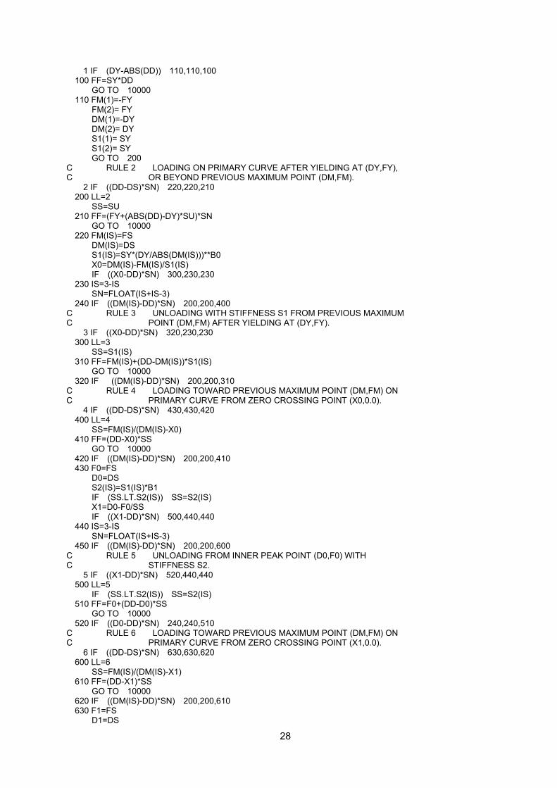
28

1 IF (DY-ABS(DD)) 110,110,100 100 FF=SY*DD GO TO 10000 110 FM(1)=-FY FM(2)= FY DM(1)=-DY DM(2)= DY S1(1)= SY S1(2)= SY GO TO 200 C RULE 2 LOADING ON PRIMARY CURVE AFTER YIELDING AT (DY,FY), C OR BEYOND PREVIOUS MAXIMUM POINT (DM,FM). 2 IF ((DD-DS)*SN) 220,220,210 200 LL=2 SS=SU 210 FF=(FY+(ABS(DD)-DY)*SU)*SN GO TO 10000 220 FM(IS)=FS DM(IS)=DS S1(IS)=SY*(DY/ABS(DM(IS)))**B0 X0=DM(IS)-FM(IS)/S1(IS) IF ((X0-DD)*SN) 300,230,230 230 IS=3-IS SN=FLOAT(IS+IS-3) 240 IF ((DM(IS)-DD)*SN) 200,200,400 C RULE 3 UNLOADING WITH STIFFNESS S1 FROM PREVIOUS MAXIMUM C POINT (DM,FM) AFTER YIELDING AT (DY,FY). 3 IF ((X0-DD)*SN) 320,230,230 300 LL=3 SS=S1(IS) 310 FF=FM(IS)+(DD-DM(IS))*S1(IS) GO TO 10000 320 IF ((DM(IS)-DD)*SN) 200,200,310 C RULE 4 LOADING TOWARD PREVIOUS MAXIMUM POINT (DM,FM) ON C PRIMARY CURVE FROM ZERO CROSSING POINT (X0,0.0). 4 IF ((DD-DS)*SN) 430,430,420 400 LL=4 SS=FM(IS)/(DM(IS)-X0) 410 FF=(DD-X0)*SS GO TO 10000 420 IF ((DM(IS)-DD)*SN) 200,200,410 430 F0=FS D0=DS S2(IS)=S1(IS)*B1 IF (SS.LT.S2(IS)) SS=S2(IS) X1=D0-F0/SS IF ((X1-DD)*SN) 500,440,440 440 IS=3-IS SN=FLOAT(IS+IS-3) 450 IF ((DM(IS)-DD)*SN) 200,200,600 C RULE 5 UNLOADING FROM INNER PEAK POINT (D0,F0) WITH C STIFFNESS S2. 5 IF ((X1-DD)*SN) 520,440,440 500 LL=5 IF (SS.LT.S2(IS)) SS=S2(IS) 510 FF=F0+(DD-D0)*SS GO TO 10000 520 IF ((D0-DD)*SN) 240,240,510 C RULE 6 LOADING TOWARD PREVIOUS MAXIMUM POINT (DM,FM) ON C PRIMARY CURVE FROM ZERO CROSSING POINT (X1,0.0). 6 IF ((DD-DS)*SN) 630,630,620 600 LL=6 SS=FM(IS)/(DM(IS)-X1) 610 FF=(DD-X1)*SS GO TO 10000 620 IF ((DM(IS)-DD)*SN) 200,200,610 630 F1=FS D1=DS

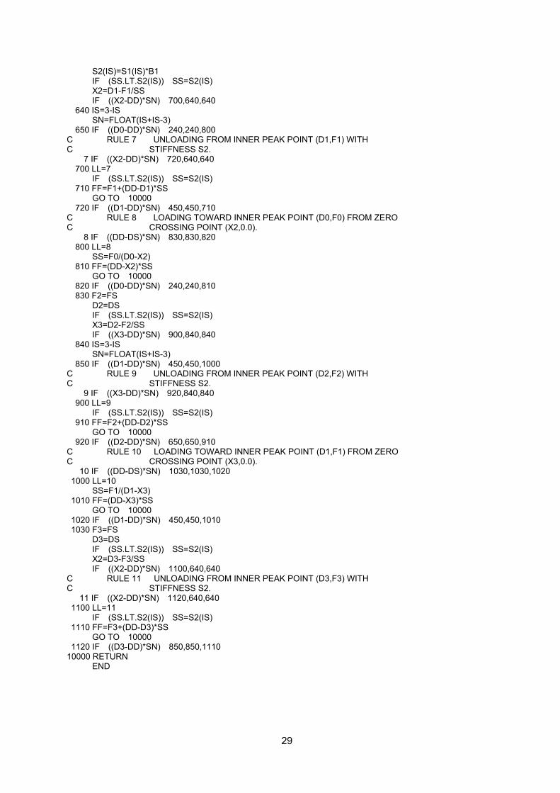
29

S2(IS)=S1(IS)*B1 IF (SS.LT.S2(IS)) SS=S2(IS) X2=D1-F1/SS IF ((X2-DD)*SN) 700,640,640 640 IS=3-IS SN=FLOAT(IS+IS-3) 650 IF ((D0-DD)*SN) 240,240,800 C RULE 7 UNLOADING FROM INNER PEAK POINT (D1,F1) WITH C STIFFNESS S2. 7 IF ((X2-DD)*SN) 720,640,640 700 LL=7 IF (SS.LT.S2(IS)) SS=S2(IS) 710 FF=F1+(DD-D1)*SS GO TO 10000 720 IF ((D1-DD)*SN) 450,450,710 C RULE 8 LOADING TOWARD INNER PEAK POINT (D0,F0) FROM ZERO C CROSSING POINT (X2,0.0). 8 IF ((DD-DS)*SN) 830,830,820 800 LL=8 SS=F0/(D0-X2) 810 FF=(DD-X2)*SS GO TO 10000 820 IF ((D0-DD)*SN) 240,240,810 830 F2=FS D2=DS IF (SS.LT.S2(IS)) SS=S2(IS) X3=D2-F2/SS IF ((X3-DD)*SN) 900,840,840 840 IS=3-IS SN=FLOAT(IS+IS-3) 850 IF ((D1-DD)*SN) 450,450,1000 C RULE 9 UNLOADING FROM INNER PEAK POINT (D2,F2) WITH C STIFFNESS S2. 9 IF ((X3-DD)*SN) 920,840,840 900 LL=9 IF (SS.LT.S2(IS)) SS=S2(IS) 910 FF=F2+(DD-D2)*SS GO TO 10000 920 IF ((D2-DD)*SN) 650,650,910 C RULE 10 LOADING TOWARD INNER PEAK POINT (D1,F1) FROM ZERO C CROSSING POINT (X3,0.0). 10 IF ((DD-DS)*SN) 1030,1030,1020 1000 LL=10 SS=F1/(D1-X3) 1010 FF=(DD-X3)*SS GO TO 10000 1020 IF ((D1-DD)*SN) 450,450,1010 1030 F3=FS D3=DS IF (SS.LT.S2(IS)) SS=S2(IS) X2=D3-F3/SS IF ((X2-DD)*SN) 1100,640,640 C RULE 11 UNLOADING FROM INNER PEAK POINT (D3,F3) WITH C STIFFNESS S2. 11 IF ((X2-DD)*SN) 1120,640,640 1100 LL=11 IF (SS.LT.S2(IS)) SS=S2(IS) 1110 FF=F3+(DD-D3)*SS GO TO 10000 1120 IF ((D3-DD)*SN) 850,850,1110 10000 RETURN END

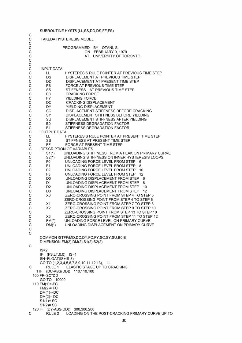
30

SUBROUTINE HYST5 (LL,SS,DD,DS,FF,FS) C C TAKEDA HYSTERESIS MODEL C C PROGRAMMED BY OTANI, S. C ON FEBRUARY 9, 1979 C AT UNIVERSITY OF TORONTO C C C INPUT DATA C LL HYSTERESIS RULE POINTER AT PREVIOUS TIME STEP C DS DISPLACEMENT AT PREVIOUS TIME STEP C DD DISPLACEMENT AT PRESENT TIME STEP C FS FORCE AT PREVIOUS TIME STEP C SS STIFFNESS AT PREVIOUS TIME STEP C FC CRACKING FORCE C FY YIELDING FORCE C DC CRACKING DISPLACEMENT C DY YIELDING DISPLACEMENT C SC DISPLACEMENT STIFFNESS BEFORE CRACKING C SY DISPLACEMENT STIFFNESS BEFORE YIELDING C SU DISPLACEMENT STIFFNESS AFTER YIELDING C B0 STIFFNESS DEGRADATION FACTOR C B1 STIFFNESS DEGRADATION FACTOR C OUTPUT DATA C LL HYSTERESIS RULE POINTER AT PRESENT TIME STEP C SS STIFFNESS AT PRESENT TIME STEP C FF FORCE AT PRESENT TIME STEP C DESCRIPTION OF VARIABLES C S1(*) UNLOADING STIFFNESS FROM A PEAK ON PRIMARY CURVE C S2(*) UNLOADING STIFFNESS ON INNER HYSTERESIS LOOPS C F0 UNLOADING FORCE LEVEL FROM STEP 6 C F1 UNLOADING FORCE LEVEL FROM STEP 8 C F2 UNLOADING FORCE LEVEL FROM STEP 10 C F3 UNLOADING FORCE LEVEL FROM STEP 12 C D0 UNLOADING DISPLACEMENT FROM STEP 6 C D1 UNLOADING DISPLACEMENT FROM STEP 8 C D2 UNLOADING DISPLACEMENT FROM STEP 10 C D3 UNLOADING DISPLACEMENT FROM STEP 12 C X0 ZERO-CROSSING POINT FROM STEP 4 TO STEP 5 C ZERO-CROSSING POINT FROM STEP 4 TO STEP 6 C X1 ZERO-CROSSING POINT FROM STEP 7 TO STEP 8 C X2 ZERO-CROSSING POINT FROM STEP 9 TO STEP 10 C ZERO-CROSSING POINT FROM STEP 13 TO STEP 10 C X3 ZERO-CROSSING POINT FROM STEP 11 TO STEP 12 C FM(*) UNLOADING FORCE LEVEL ON PRIMARY CURVE C DM(*) UNLOADING DISPLACEMENT ON PRIMARY CURVE C C COMMON /STFF/MD,DC,DY,FC,FY,SC,SY,SU,B0,B1 DIMENSION FM(2),DM(2),S1(2),S2(2) C IS=2 IF (FS.LT.0.0) IS=1 SN=FLOAT(IS+IS-3) GO TO (1,2,3,4,5,6,7,8,9,10,11,12,13), LL C RULE 1 ELASTIC STAGE UP TO CRACKING 1 IF (DC-ABS(DD)) 110,110,100 100 FF=SC*DD GO TO 10000 110 FM(1)=-FC FM(2)= FC DM(1)=-DC DM(2)= DC S1(1)= SC S1(2)= SC 120 IF (DY-ABS(DD)) 300,300,200 C RULE 2 LOADING ON THE POST-CRACKING FRIMARY CURVE UP TO

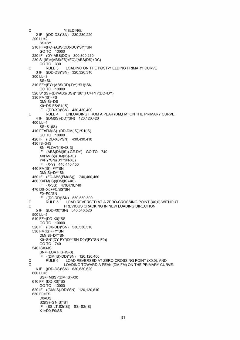
31

C YIELDING. 2 IF ((DD-DS)*SN) 230,230,220 200 LL=2 SS=SY 210 FF=(FC+(ABS(DD)-DC)*SY)*SN GO TO 10000 220 IF (DY-ABS(DD)) 300,300,210 230 S1(IS)=(ABS(FS)+FC)/(ABS(DS)+DC) GO TO 330 C RULE 3 LOADING ON THE POST-YIELDING PRIMARY CURVE 3 IF ((DD-DS)*SN) 320,320,310 300 LL=3 SS=SU 310 FF=(FY+(ABS(DD)-DY)*SU)*SN GO TO 10000 320 S1(IS)=(DY/ABS(DS))**B0*(FC+FY)/(DC+DY) 330 FM(IS)=FS DM(IS)=DS X0=DS-FS/S1(IS) IF ((DD-X0)*SN) 430,430,400 C RULE 4 UNLOADING FROM A PEAK (DM,FM) ON THE PRIMARY CURVE. 4 IF ((DM(IS)-DD)*SN) 120,120,420 400 LL=4 SS=S1(IS) 410 FF=FM(IS)+(DD-DM(IS))*S1(IS) GO TO 10000 420 IF ((DD-X0)*SN) 430,430,410 430 IS=3-IS SN=FLOAT(IS+IS-3) IF (ABS(DM(IS)).GE.DY) GO TO 740 X=FM(IS)/(DM(IS)-X0) Y=FY*SN/(DY*SN-X0) IF (X-Y) 440,440,450 440 FM(IS)=FY*SN DM(IS)=DY*SN 450 IF (FC-ABS(FM(IS))) 740,460,460 460 X=FM(IS)/(DM(IS)-X0) IF (X-SS) 470,470,740 470 D0=X0+FC/SS*SN F0=FC*SN IF ((D0-DD)*SN) 530,530,500 C RULE 5 LOAD REVERSED AT A ZERO-CROSSING POINT (X0,0) WITHOUT C PREVIOUS CRACKING IN NEW LOADING DIRECTION. 5 IF ((DD-X0)*SN) 540,540,520 500 LL=5 510 FF=(DD-X0)*SS GO TO 10000 520 IF ((D0-DD)*SN) 530,530,510 530 FM(IS)=FY*SN DM(IS)=DY*SN X0=SN*(DY-FY*(DY*SN-D0)/(FY*SN-F0)) GO TO 740 540 IS=3-IS SN=FLOAT(IS+IS-3) IF ((DM(IS)-DD)*SN) 120,120,400 C RULE 6 LOAD REVERSED AT ZERO-CROSSING POINT (X0,0), AND C LOADING TOWARD A PEAK (DM,FM) ON THE PRIMARY CURVE. 6 IF ((DD-DS)*SN) 630,630,620 600 LL=6 SS=FM(IS)/(DM(IS)-X0) 610 FF=(DD-X0)*SS GO TO 10000 620 IF ((DM(IS)-DD)*SN) 120,120,610 630 F0=FS D0=DS S2(IS)=S1(IS)*B1 IF (SS.LT.S2(IS)) SS=S2(IS) X1=D0-F0/SS

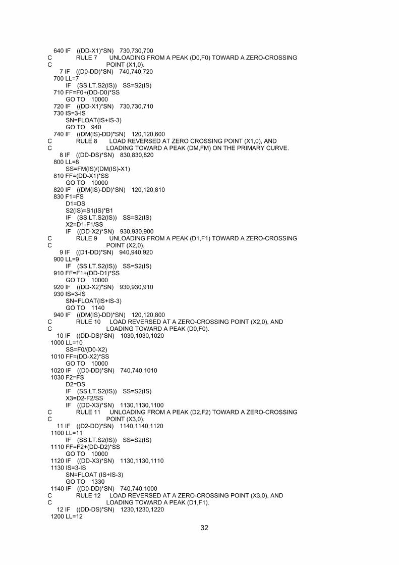
32

640 IF ((DD-X1)*SN) 730,730,700 C RULE 7 UNLOADING FROM A PEAK (D0,F0) TOWARD A ZERO-CROSSING C POINT (X1,0). 7 IF ((D0-DD)*SN) 740,740,720 700 LL=7 IF (SS.LT.S2(IS)) SS=S2(IS) 710 FF=F0+(DD-D0)*SS GO TO 10000 720 IF ((DD-X1)*SN) 730,730,710 730 IS=3-IS SN=FLOAT(IS+IS-3) GO TO 940 740 IF ((DM(IS)-DD)*SN) 120,120,600 C RULE 8 LOAD REVERSED AT ZERO CROSSING POINT (X1,0), AND C LOADING TOWARD A PEAK (DM,FM) ON THE PRIMARY CURVE. 8 IF ((DD-DS)*SN) 830,830,820 800 LL=8 SS=FM(IS)/(DM(IS)-X1) 810 FF=(DD-X1)*SS GO TO 10000 820 IF ((DM(IS)-DD)*SN) 120,120,810 830 F1=FS D1=DS S2(IS)=S1(IS)*B1 IF (SS.LT.S2(IS)) SS=S2(IS) X2=D1-F1/SS IF ((DD-X2)*SN) 930,930,900 C RULE 9 UNLOADING FROM A PEAK (D1,F1) TOWARD A ZERO-CROSSING C POINT (X2,0). 9 IF ((D1-DD)*SN) 940,940,920 900 LL=9 IF (SS.LT.S2(IS)) SS=S2(IS) 910 FF=F1+(DD-D1)*SS GO TO 10000 920 IF ((DD-X2)*SN) 930,930,910 930 IS=3-IS SN=FLOAT(IS+IS-3) GO TO 1140 940 IF ((DM(IS)-DD)*SN) 120,120,800 C RULE 10 LOAD REVERSED AT A ZERO-CROSSING POINT (X2,0), AND C LOADING TOWARD A PEAK (D0,F0). 10 IF ((DD-DS)*SN) 1030,1030,1020 1000 LL=10 SS=F0/(D0-X2) 1010 FF=(DD-X2)*SS GO TO 10000 1020 IF ((D0-DD)*SN) 740,740,1010 1030 F2=FS D2=DS IF (SS.LT.S2(IS)) SS=S2(IS) X3=D2-F2/SS IF ((DD-X3)*SN) 1130,1130,1100 C RULE 11 UNLOADING FROM A PEAK (D2,F2) TOWARD A ZERO-CROSSING C POINT (X3,0). 11 IF ((D2-DD)*SN) 1140,1140,1120 1100 LL=11 IF (SS.LT.S2(IS)) SS=S2(IS) 1110 FF=F2+(DD-D2)*SS GO TO 10000 1120 IF ((DD-X3)*SN) 1130,1130,1110 1130 IS=3-IS SN=FLOAT (IS+IS-3) GO TO 1330 1140 IF ((D0-DD)*SN) 740,740,1000 C RULE 12 LOAD REVERSED AT A ZERO-CROSSING POINT (X3,0), AND C LOADING TOWARD A PEAK (D1,F1). 12 IF ((DD-DS)*SN) 1230,1230,1220 1200 LL=12

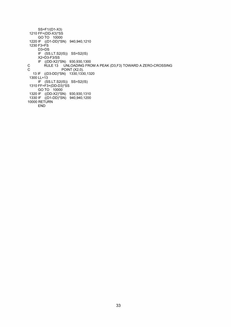
33

SS=F1/(D1-X3) 1210 FF=(DD-X3)*SS GO TO 10000 1220 IF ((D1-DD)*SN) 940,940,1210 1230 F3=FS D3=DS IF (SS.LT.S2(IS)) SS=S2(IS) X2=D3-F3/SS IF ((DD-X2)*SN) 930,930,1300 C RULE 13 UNLOADING FROM A PEAK (D3,F3) TOWARD A ZERO-CROSSING C POINT (X2,0). 13 IF ((D3-DD)*SN) 1330,1330,1320 1300 LL=13 IF (SS.LT.S2(IS)) SS=S2(IS) 1310 FF=F3+(DD-D3)*SS GO TO 10000 1320 IF ((DD-X2)*SN) 930,930,1310 1330 IF ((D1-DD)*SN) 940,940,1200 10000 RETURN END

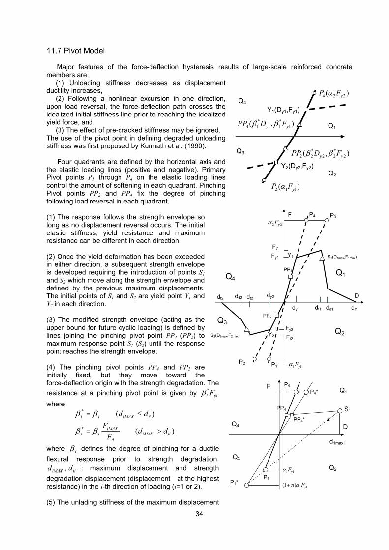
34

11.7 Pivot Model

Major features of the force-deflection hysteresis results of large-scale reinforced concrete members are;

(1) Unloading stiffness decreases as displacement ductility increases,

(2) Following a nonlinear excursion in one direction, upon load reversal, the force-deflection path crosses the idealized initial stiffness line prior to reaching the idealized yield force, and

(3) The effect of pre-cracked stiffness may be ignored. The use of the pivot point in defining degraded unloading stiffness was first proposed by Kunnath et al. (1990).

Four quadrants are defined by the horizontal axis and the elastic loading lines (positive and negative). Primary Pivot points P1 through P4 on the elastic loading lines control the amount of softening in each quadrant. Pinching Pivot points PP2 and PP4 fix the degree of pinching following load reversal in each quadrant. (1) The response follows the strength envelope so long as no displacement reversal occurs. The initial elastic stiffness, yield resistance and maximum resistance can be different in each direction. (2) Once the yield deformation has been exceeded in either direction, a subsequent strength envelope is developed requiring the introduction of points S1 and S2 which move along the strength envelope and defined by the previous maximum displacements. The initial points of S1 and S2 are yield point Y1 and Y2 in each direction. (3) The modified strength envelope (acting as the upper bound for future cyclic loading) is defined by lines joining the pinching pivot point PP4 (PP2) to maximum response point S1 (S2) until the response point reaches the strength envelope. (4) The pinching pivot points PP4 and PP2 are initially fixed, but they move toward the force-deflection origin with the strength degradation. The resistance at a pinching pivot point is given by *

i yiFβ where

)(

)(

*

*

tiiMAXti

iMAXii

tiiMAXii

ddF

Fdd

>=

≤=

ββ

ββ

where iβ defines the degree of pinching for a ductile flexural response prior to strength degradation.

tiiMAX dd , : maximum displacement and strength degradation displacement (displacement at the highest resistance) in the i-th direction of loading (i=1 or 2). (5) The unlading stiffness of the maximum displacement

Q1

Q2

Q3

Q44 2 2( )yP Fα

2 1 1( )yP Fα

Y2(Dy2,Fy2)

Y1(Dy1,Fy1) * *

4 1 1 1 1( , )y yPP D Fβ β

* *2 2 2 2 2( , )y yPP D Fβ β

Q1

Q2

Q4

Q3

D

F

Y1

Y2

P1

P4 P3

P2

dy dt1 dd1 df1

Fy1

Fy2

dy2

2 2yFα

1 1yFα

dt2dd2df2

PP4

PP2

Ft1

Ft2

S1(D1max,F1max)

S2(D2max,F2max)

Q2 Q3

Q4

Q1

S1

d1max

D

PP4

PP4*

1 1yFα

1 1(1 ) yFη α+ P1

P1*

F P4 P4*

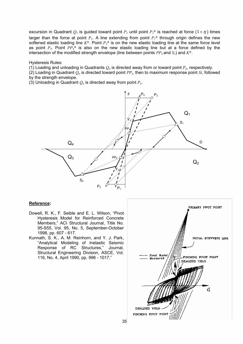
35

excursion in Quadrant Q1 is guided toward point P1 until point P1* is reached at force ( η+1 ) times larger than the force at point P1. A line extending from point P1* through origin defines the new softened elastic loading line K*. Point P4* is on the new elastic loading line at the same force level as point P4. Point PP4* is also on the new elastic loading line but at a force defined by the intersection of the modified strength envelope (line between points PP4 and S1) and K*. Hysteresis Rules: (1) Loading and unloading in Quadrants Qn is directed away from or toward point Pn, respectively. (2) Loading in Quadrant Qn is directed toward point PPn, then to maximum response point Si, followed by the strength envelope. (3) Unloading in Quadrant Qn is directed away from point Pn.

Reference: Dowell, R. K., F. Seible and E. L. Wilson, “Pivot

Hysteresis Model for Reinforced Concrete Members,” ACI Structural Journal, Title No. 95-S55, Vol. 95, No. 5, September-October 1998, pp. 607 - 617.

Kunnath, S. K., A. M. Reinhorn, and Y. J. Park, “Analytical Modeling of Inelastic Seismic Response of RC Structures,” Journal, Structural Engineering Division, ASCE, Vol. 116, No. 4, April 1990, pp. 996 - 1017,”

Q1

Q2

Q4

Q3

D

F

Y1

Y2

P1

P4 P3

P2

PP4

PP2

S1

S2

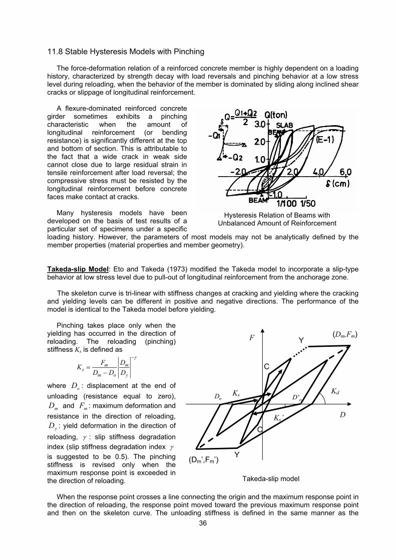
36

11.8 Stable Hysteresis Models with Pinching

The force-deformation relation of a reinforced concrete member is highly dependent on a loading history, characterized by strength decay with load reversals and pinching behavior at a low stress level during reloading, when the behavior of the member is dominated by sliding along inclined shear cracks or slippage of longitudinal reinforcement.

A flexure-dominated reinforced concrete girder sometimes exhibits a pinching characteristic when the amount of longitudinal reinforcement (or bending resistance) is significantly different at the top and bottom of section. This is attributable to the fact that a wide crack in weak side cannot close due to large residual strain in tensile reinforcement after load reversal; the compressive stress must be resisted by the longitudinal reinforcement before concrete faces make contact at cracks.

Many hysteresis models have been developed on the basis of test results of a particular set of specimens under a specific loading history. However, the parameters of most models may not be analytically defined by the member properties (material properties and member geometry). Takeda-slip Model: Eto and Takeda (1973) modified the Takeda model to incorporate a slip-type behavior at low stress level due to pull-out of longitudinal reinforcement from the anchorage zone.

The skeleton curve is tri-linear with stiffness changes at cracking and yielding where the cracking and yielding levels can be different in positive and negative directions. The performance of the model is identical to the Takeda model before yielding.

Pinching takes place only when the yielding has occurred in the direction of reloading. The reloading (pinching) stiffness Ks is defined as

m ms

m o y

F DKD D D

γ−

=−

where oD : displacement at the end of unloading (resistance equal to zero),

mD and mF : maximum deformation and resistance in the direction of reloading,

yD : yield deformation in the direction of reloading, γ : slip stiffness degradation index (slip stiffness degradation index γ is suggested to be 0.5). The pinching stiffness is revised only when the maximum response point is exceeded in the direction of reloading.

When the response point crosses a line connecting the origin and the maximum response point in the direction of reloading, the response point moved toward the previous maximum response point and then on the skeleton curve. The unloading stiffness is defined in the same manner as the

D

F Y (Dm,Fm)

KdoD

C

C

Y

Ks

Ks’

(Dm’,Fm’)

'oD

Takeda-slip model

Hysteresis Relation of Beams with Unbalanced Amount of Reinforcement

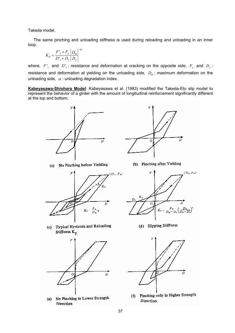
37

Takeda model. The same pinching and unloading stiffness is used during reloading and unloading in an inner

loop.

''c y m

dc y y

F F DKD D D

α−+

=+

where, 'cF and 'cD : resistance and deformation at cracking on the opposite side, yF and yD :

resistance and deformation at yielding on the unloading side, mD : maximum deformation on the unloading side, α : unloading degradation index. Kabeyasawa-Shiohara Model: Kabeyasawa et al. (1983) modified the Takeda-Eto slip model to represent the behavior of a girder with the amount of longitudinal reinforcement significantly different at the top and bottom;

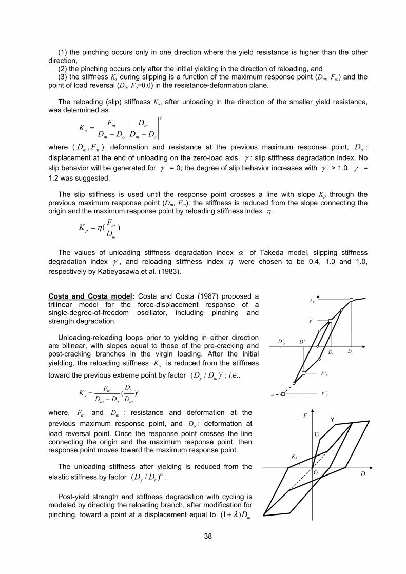
38

(1) the pinching occurs only in one direction where the yield resistance is higher than the other direction,

(2) the pinching occurs only after the initial yielding in the direction of reloading, and (3) the stiffness Ks during slipping is a function of the maximum response point (Dm, Fm) and the

point of load reversal (Do, Fo=0.0) in the resistance-deformation plane.

The reloading (slip) stiffness Ks, after unloading in the direction of the smaller yield resistance, was determined as

γ

om

m

om

ms DD

DDD

FK−−

=

where ( mm FD , ): deformation and resistance at the previous maximum response point, oD : displacement at the end of unloading on the zero-load axis, γ : slip stiffness degradation index. No slip behavior will be generated for γ = 0; the degree of slip behavior increases with γ > 1.0. γ = 1.2 was suggested.

The slip stiffness is used until the response point crosses a line with slope Kp through the previous maximum response point (Dm, Fm); the stiffness is reduced from the slope connecting the origin and the maximum response point by reloading stiffness index η ,

)(m

mp D

FK η=

The values of unloading stiffness degradation index α of Takeda model, slipping stiffness

degradation index γ , and reloading stiffness index η were chosen to be 0.4, 1.0 and 1.0, respectively by Kabeyasawa et al. (1983). Costa and Costa model: Costa and Costa (1987) proposed a trilinear model for the force-displacement response of a single-degree-of-freedom oscillator, including pinching and strength degradation.

Unloading-reloading loops prior to yielding in either direction are bilinear, with slopes equal to those of the pre-cracking and post-cracking branches in the virgin loading. After the initial yielding, the reloading stiffness sK is reduced from the stiffness

toward the previous extreme point by factor ( / )y mD D γ ; i.e.,

( )yms

m o m

DFKD D D

γ=−

where, mF and mD : resistance and deformation at the previous maximum response point, and oD : deformation at load reversal point. Once the response point crosses the line connecting the origin and the maximum response point, then response point moves toward the maximum response point.

The unloading stiffness after yielding is reduced from the elastic stiffness by factor ( / )y rD D α .

Post-yield strength and stiffness degradation with cycling is modeled by directing the reloading branch, after modification for pinching, toward a point at a displacement equal to (1 ) mDλ+

D

F

C

Y

Ks

O

Dc Dy

Fc

Fy

F’c

F’y

D’c D’y

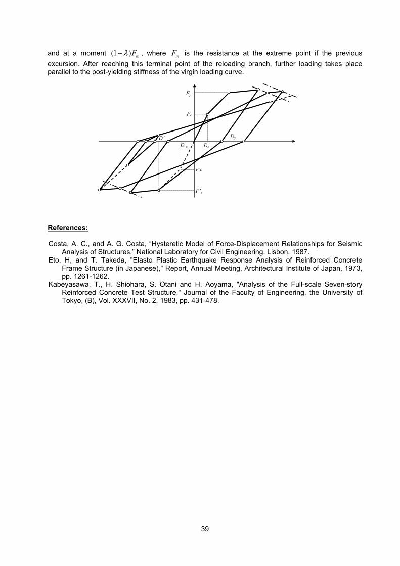
39

and at a moment (1 ) mFλ− , where mF is the resistance at the extreme point if the previous excursion. After reaching this terminal point of the reloading branch, further loading takes place parallel to the post-yielding stiffness of the virgin loading curve.

References: Costa, A. C., and A. G. Costa, “Hysteretic Model of Force-Displacement Relationships for Seismic

Analysis of Structures,” National Laboratory for Civil Engineering, Lisbon, 1987. Eto, H, and T. Takeda, "Elasto Plastic Earthquake Response Analysis of Reinforced Concrete

Frame Structure (in Japanese)," Report, Annual Meeting, Architectural Institute of Japan, 1973, pp. 1261-1262.

Kabeyasawa, T., H. Shiohara, S. Otani and H. Aoyama, "Analysis of the Full-scale Seven-story Reinforced Concrete Test Structure," Journal of the Faculty of Engineering, the University of Tokyo, (B), Vol. XXXVII, No. 2, 1983, pp. 431-478.

F’c

F’y

D’c

D’y

Dc

Dy

Fc

Fy

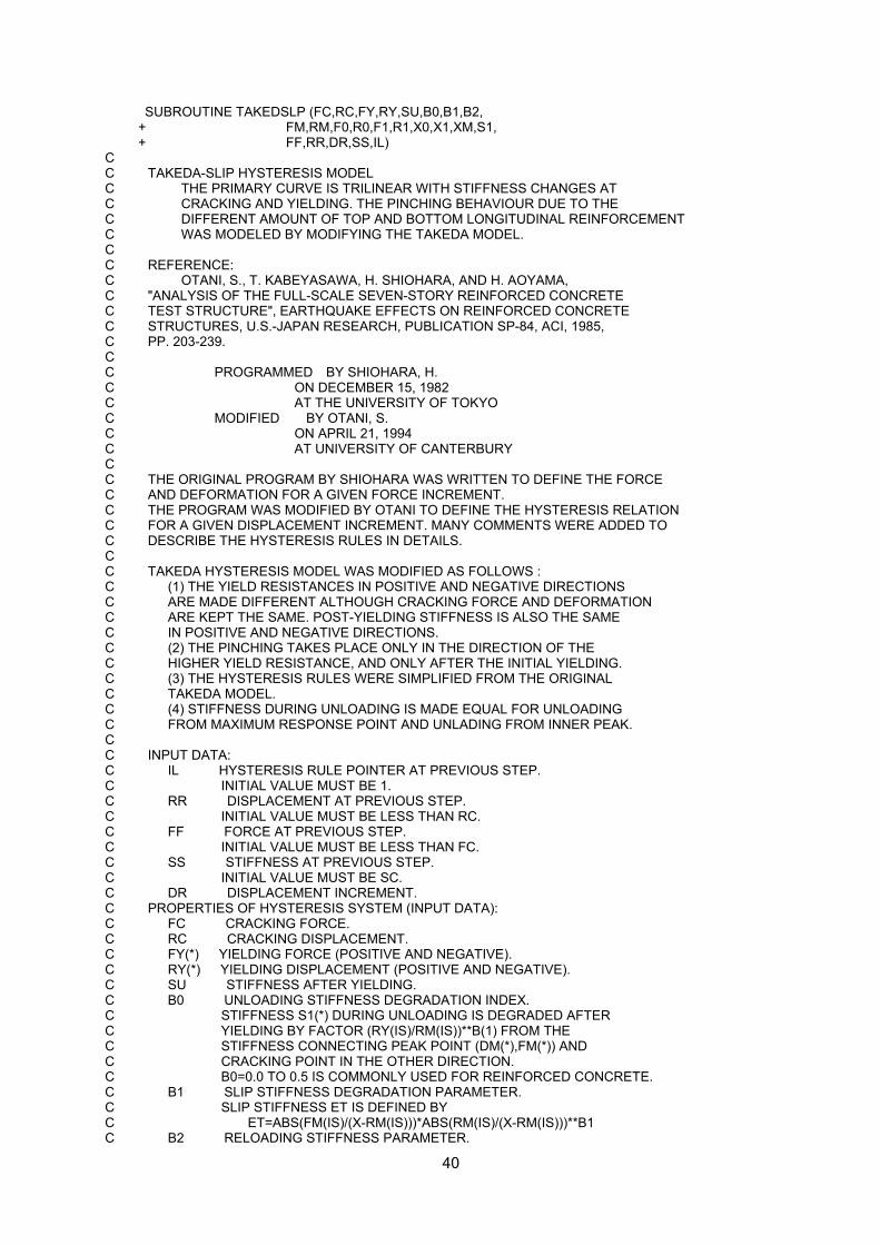
40

SUBROUTINE TAKEDSLP (FC,RC,FY,RY,SU,B0,B1,B2, + FM,RM,F0,R0,F1,R1,X0,X1,XM,S1, + FF,RR,DR,SS,IL) C C TAKEDA-SLIP HYSTERESIS MODEL C THE PRIMARY CURVE IS TRILINEAR WITH STIFFNESS CHANGES AT C CRACKING AND YIELDING. THE PINCHING BEHAVIOUR DUE TO THE C DIFFERENT AMOUNT OF TOP AND BOTTOM LONGITUDINAL REINFORCEMENT C WAS MODELED BY MODIFYING THE TAKEDA MODEL. C C REFERENCE: C OTANI, S., T. KABEYASAWA, H. SHIOHARA, AND H. AOYAMA, C "ANALYSIS OF THE FULL-SCALE SEVEN-STORY REINFORCED CONCRETE C TEST STRUCTURE", EARTHQUAKE EFFECTS ON REINFORCED CONCRETE C STRUCTURES, U.S.-JAPAN RESEARCH, PUBLICATION SP-84, ACI, 1985, C PP. 203-239. C C PROGRAMMED BY SHIOHARA, H. C ON DECEMBER 15, 1982 C AT THE UNIVERSITY OF TOKYO C MODIFIED BY OTANI, S. C ON APRIL 21, 1994 C AT UNIVERSITY OF CANTERBURY C C THE ORIGINAL PROGRAM BY SHIOHARA WAS WRITTEN TO DEFINE THE FORCE C AND DEFORMATION FOR A GIVEN FORCE INCREMENT. C THE PROGRAM WAS MODIFIED BY OTANI TO DEFINE THE HYSTERESIS RELATION C FOR A GIVEN DISPLACEMENT INCREMENT. MANY COMMENTS WERE ADDED TO C DESCRIBE THE HYSTERESIS RULES IN DETAILS. C C TAKEDA HYSTERESIS MODEL WAS MODIFIED AS FOLLOWS : C (1) THE YIELD RESISTANCES IN POSITIVE AND NEGATIVE DIRECTIONS C ARE MADE DIFFERENT ALTHOUGH CRACKING FORCE AND DEFORMATION C ARE KEPT THE SAME. POST-YIELDING STIFFNESS IS ALSO THE SAME C IN POSITIVE AND NEGATIVE DIRECTIONS. C (2) THE PINCHING TAKES PLACE ONLY IN THE DIRECTION OF THE C HIGHER YIELD RESISTANCE, AND ONLY AFTER THE INITIAL YIELDING. C (3) THE HYSTERESIS RULES WERE SIMPLIFIED FROM THE ORIGINAL C TAKEDA MODEL. C (4) STIFFNESS DURING UNLOADING IS MADE EQUAL FOR UNLOADING C FROM MAXIMUM RESPONSE POINT AND UNLADING FROM INNER PEAK. C C INPUT DATA: C IL HYSTERESIS RULE POINTER AT PREVIOUS STEP. C INITIAL VALUE MUST BE 1. C RR DISPLACEMENT AT PREVIOUS STEP. C INITIAL VALUE MUST BE LESS THAN RC. C FF FORCE AT PREVIOUS STEP. C INITIAL VALUE MUST BE LESS THAN FC. C SS STIFFNESS AT PREVIOUS STEP. C INITIAL VALUE MUST BE SC. C DR DISPLACEMENT INCREMENT. C PROPERTIES OF HYSTERESIS SYSTEM (INPUT DATA): C FC CRACKING FORCE. C RC CRACKING DISPLACEMENT. C FY(*) YIELDING FORCE (POSITIVE AND NEGATIVE). C RY(*) YIELDING DISPLACEMENT (POSITIVE AND NEGATIVE). C SU STIFFNESS AFTER YIELDING. C B0 UNLOADING STIFFNESS DEGRADATION INDEX. C STIFFNESS S1(*) DURING UNLOADING IS DEGRADED AFTER C YIELDING BY FACTOR (RY(IS)/RM(IS))**B(1) FROM THE C STIFFNESS CONNECTING PEAK POINT (DM(*),FM(*)) AND C CRACKING POINT IN THE OTHER DIRECTION. C B0=0.0 TO 0.5 IS COMMONLY USED FOR REINFORCED CONCRETE. C B1 SLIP STIFFNESS DEGRADATION PARAMETER. C SLIP STIFFNESS ET IS DEFINED BY C ET=ABS(FM(IS)/(X-RM(IS)))*ABS(RM(IS)/(X-RM(IS)))**B1 C B2 RELOADING STIFFNESS PARAMETER.

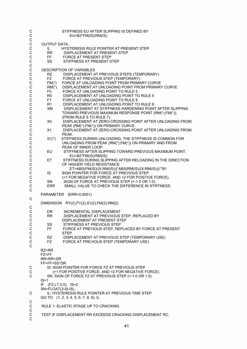
41

C STIFFNESS EU AFTER SLIPPING IS DEFINED BY C EU=B2*FM(IS)/RM(IS) C C OUTPUT DATA: C IL HYSTERESIS RULE POINTER AT PRESENT STEP C RR DISPLACEMENT AT PRESENT STEP C FF FORCE AT PRESENT STEP C SS STIFFNESS AT PRESENT STEP C C DESCRIPTION OF VARIABLES C RZ DISPLACEMENT AT PREVIOUS STEPS (TEMPORARY) C FZ FORCE AT PREVIOUS STEP (TEMPORARY) C FM(*) FORCE AT UNLOADING POINT FROM PRIMARY CURVE C RM(*) DISPLACEMENT AT UNLOADING POINT FROM PRIMARY CURVE C F0 FORCE AT UNLOADING POINT TO RULE 5 C R0 DISPLACEMENT AT UNLOADING POINT TO RULE 5 C F1 FORCE AT UNLOADING POINT TO RULE 8 C R1 DISPLACEMENT AT UNLOADING POINT TO RULE 8 C XM DISPLACEMENT AT STIFFNESS HARDENING POINT AFTER SLIPPING C TOWARD PREVIOUS MAXIMUM RESPONSE POINT (RM(*),FM(*)), C (FROM RULE 6 TO RULE 7). C X0 DISPLACEMENT AT ZERO-CROSSING POINT AFTER UNLOADING FROM C PEAK (RM(*),FM(*)) ON PRIMARY CURVE. C X1 DISPLACEMENT AT ZERO-CROSSING POINT AFTER UNLOADING FROM C PEAK. C S1(*) STIFFNESS DURING UNLOADING; THE STIFFNESS IS COMMON FOR C UNLOADING FROM PEAK (RM(*),FM(*)) ON PRIMARY AND FROM C PEAK OF INNER LOOP. C EU STIFFNESS AFTER SLIPPING TOWARD PREVIOUS MAXIMUM POINT. C EU=B2*FM(IS)/RM(IS) C ET STIFFNESS DURING SLIPPING AFTER RELOADING IN THE DIRECTION C OF HIGHER YIELD RESISTANCE. C ET=ABS(FM(IS)/(X-RM(IS)))*ABS(RM(IS)/(X-RM(IS)))**B1 C IS SIGN POINTER FOR FORCE AT PREVIOUS STEP. C (=1 FOR NEGATIVE FORCE, AND =2 FOR POISTIVE FORCE). C SN SIGN OF FORCE AT PREVIOUS STEP (=-1.0 OR 1.0). C ERR SMALL VALUE TO CHECK THE DIFFERENCE IN STIFFNESS. C PARAMETER (ERR=0.0001) C DIMENSION RY(2),FY(2),S1(2),FM(2),RM(2) C C DR INCREMENTAL DISPLACEMENT C RR DISPLACEMENT AT PREVIIOUS STEP, REPLACED BY C DISPLACEMENT AT PRESENT STEP C SS STIFFNESS AT PREVIOUS STEP C FF FORCE AT PREVIOUS STEP, REPLACED BY FORCE AT PRESENT C STEP C RZ DISPLACEMENT AT PREVIOUS STEP (TEMPORARY USE) C FZ FORCE AT PREVIOUS STEP (TEMPORARY USE) C RZ=RR FZ=FF RR=RR+DR FF=FF+SS*DR C IS: SIGN POINTER FOR FORCE FZ AT PREVIOUS STEP C (=1 FOR POISTIVE FORCE, AND =2 FOR NEGATIVE FORCE) C SN: SIGN OF FORCE FZ AT PREVIOUS STEP (=-1.0 OR 1.0) IS=1 IF (FZ.LT.0.0) IS=2 SN=FLOAT(3-IS-IS) C IL: HYSTERESIS RULE POINTER AT PREVIOUS TIME STEP GO TO (1, 2, 3, 4, 5, 6, 7, 8, 9), IL C C RULE 1: ELASTIC STAGE UP TO CRACKING C C TEST IF DISPLACEMENT RR EXCEEDS CRACKING DISPLACEMENT RC. C

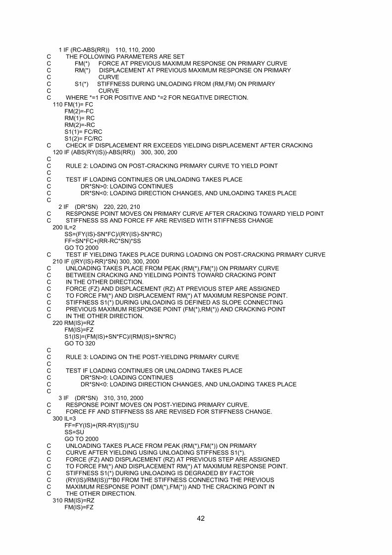
42

1 IF (RC-ABS(RR)) 110, 110, 2000 C THE FOLLOWING PARAMETERS ARE SET C FM(*) FORCE AT PREVIOUS MAXIMUM RESPONSE ON PRIMARY CURVE C RM(*) DISPLACEMENT AT PREVIOUS MAXIMUM RESPONSE ON PRIMARY C CURVE C S1(*) STIFFNESS DURING UNLOADING FROM (RM,FM) ON PRIMARY C CURVE C WHERE *=1 FOR POSITIVE AND *=2 FOR NEGATIVE DIRECTION. 110 FM(1)= FC FM(2)=-FC RM(1)= RC RM(2)=-RC S1(1)= FC/RC S1(2)= FC/RC C CHECK IF DISPLACEMENT RR EXCEEDS YIELDING DISPLACEMENT AFTER CRACKING 120 IF (ABS(RY(IS))-ABS(RR)) 300, 300, 200 C C RULE 2: LOADING ON POST-CRACKING PRIMARY CURVE TO YIELD POINT C C TEST IF LOADING CONTINUES OR UNLOADING TAKES PLACE C DR*SN>0: LOADING CONTINUES C DR*SN<0: LOADING DIRECTION CHANGES, AND UNLOADING TAKES PLACE C 2 IF (DR*SN) 220, 220, 210 C RESPONSE POINT MOVES ON PRIMARY CURVE AFTER CRACKING TOWARD YIELD POINT C STIFFNESS SS AND FORCE FF ARE REVISED WITH STIFFNESS CHANGE 200 IL=2 SS=(FY(IS)-SN*FC)/(RY(IS)-SN*RC) FF=SN*FC+(RR-RC*SN)*SS GO TO 2000 C TEST IF YIELDING TAKES PLACE DURING LOADING ON POST-CRACKING PRIMARY CURVE 210 IF ((RY(IS)-RR)*SN) 300, 300, 2000 C UNLOADING TAKES PLACE FROM PEAK (RM(*),FM(*)) ON PRIMARY CURVE C BETWEEN CRACKING AND YIELDING POINTS TOWARD CRACKING POINT C IN THE OTHER DIRECTION. C FORCE (FZ) AND DISPLACEMENT (RZ) AT PREVIOUS STEP ARE ASSIGNED C TO FORCE FM(*) AND DISPLACEMENT RM(*) AT MAXIMUM RESPONSE POINT. C STIFFNESS S1(*) DURING UNLOADING IS DEFINED AS SLOPE CONNECTING C PREVIOUS MAXIMUM RESPONSE POINT (FM(*),RM(*)) AND CRACKING POINT C IN THE OTHER DIRECTION. 220 RM(IS)=RZ FM(IS)=FZ S1(IS)=(FM(IS)+SN*FC)/(RM(IS)+SN*RC) GO TO 320 C C RULE 3: LOADING ON THE POST-YIELDING PRIMARY CURVE C C TEST IF LOADING CONTINUES OR UNLOADING TAKES PLACE C DR*SN>0: LOADING CONTINUES C DR*SN<0: LOADING DIRECTION CHANGES, AND UNLOADING TAKES PLACE C 3 IF (DR*SN) 310, 310, 2000 C RESPONSE POINT MOVES ON POST-YIEDING PRIMARY CURVE. C FORCE FF AND STIFFNESS SS ARE REVISED FOR STIFFNESS CHANGE. 300 IL=3 FF=FY(IS)+(RR-RY(IS))*SU SS=SU GO TO 2000 C UNLOADING TAKES PLACE FROM PEAK (RM(*),FM(*)) ON PRIMARY C CURVE AFTER YIELDING USING UNLOADING STIFFNESS S1(*). C FORCE (FZ) AND DISPLACEMENT (RZ) AT PREVIOUS STEP ARE ASSIGNED C TO FORCE FM(*) AND DISPLACEMENT RM(*) AT MAXIMUM RESPONSE POINT. C STIFFNESS S1(*) DURING UNLOADING IS DEGRADED BY FACTOR C (RY(IS)/RM(IS))**B0 FROM THE STIFFNESS CONNECTING THE PREVIOUS C MAXIMUM RESPONSE POINT (DM(*),FM(*)) AND THE CRACKING POINT IN C THE OTHER DIRECTION. 310 RM(IS)=RZ FM(IS)=FZ

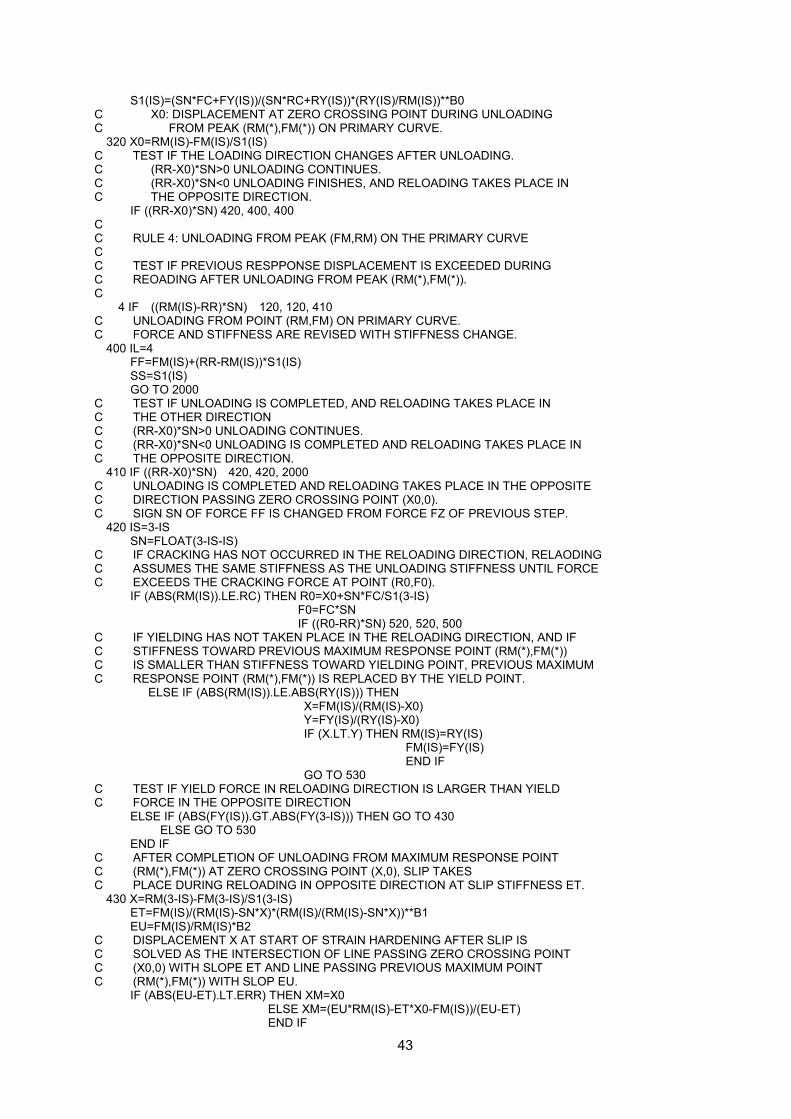
43

S1(IS)=(SN*FC+FY(IS))/(SN*RC+RY(IS))*(RY(IS)/RM(IS))**B0 C X0: DISPLACEMENT AT ZERO CROSSING POINT DURING UNLOADING C FROM PEAK (RM(*),FM(*)) ON PRIMARY CURVE. 320 X0=RM(IS)-FM(IS)/S1(IS) C TEST IF THE LOADING DIRECTION CHANGES AFTER UNLOADING. C (RR-X0)*SN>0 UNLOADING CONTINUES. C (RR-X0)*SN<0 UNLOADING FINISHES, AND RELOADING TAKES PLACE IN C THE OPPOSITE DIRECTION. IF ((RR-X0)*SN) 420, 400, 400 C C RULE 4: UNLOADING FROM PEAK (FM,RM) ON THE PRIMARY CURVE C C TEST IF PREVIOUS RESPPONSE DISPLACEMENT IS EXCEEDED DURING C REOADING AFTER UNLOADING FROM PEAK (RM(*),FM(*)). C 4 IF ((RM(IS)-RR)*SN) 120, 120, 410 C UNLOADING FROM POINT (RM,FM) ON PRIMARY CURVE. C FORCE AND STIFFNESS ARE REVISED WITH STIFFNESS CHANGE. 400 IL=4 FF=FM(IS)+(RR-RM(IS))*S1(IS) SS=S1(IS) GO TO 2000 C TEST IF UNLOADING IS COMPLETED, AND RELOADING TAKES PLACE IN C THE OTHER DIRECTION C (RR-X0)*SN>0 UNLOADING CONTINUES. C (RR-X0)*SN<0 UNLOADING IS COMPLETED AND RELOADING TAKES PLACE IN C THE OPPOSITE DIRECTION. 410 IF ((RR-X0)*SN) 420, 420, 2000 C UNLOADING IS COMPLETED AND RELOADING TAKES PLACE IN THE OPPOSITE C DIRECTION PASSING ZERO CROSSING POINT (X0,0). C SIGN SN OF FORCE FF IS CHANGED FROM FORCE FZ OF PREVIOUS STEP. 420 IS=3-IS SN=FLOAT(3-IS-IS) C IF CRACKING HAS NOT OCCURRED IN THE RELOADING DIRECTION, RELAODING C ASSUMES THE SAME STIFFNESS AS THE UNLOADING STIFFNESS UNTIL FORCE C EXCEEDS THE CRACKING FORCE AT POINT (R0,F0). IF (ABS(RM(IS)).LE.RC) THEN R0=X0+SN*FC/S1(3-IS) F0=FC*SN IF ((R0-RR)*SN) 520, 520, 500 C IF YIELDING HAS NOT TAKEN PLACE IN THE RELOADING DIRECTION, AND IF C STIFFNESS TOWARD PREVIOUS MAXIMUM RESPONSE POINT (RM(*),FM(*)) C IS SMALLER THAN STIFFNESS TOWARD YIELDING POINT, PREVIOUS MAXIMUM C RESPONSE POINT (RM(*),FM(*)) IS REPLACED BY THE YIELD POINT. ELSE IF (ABS(RM(IS)).LE.ABS(RY(IS))) THEN X=FM(IS)/(RM(IS)-X0) Y=FY(IS)/(RY(IS)-X0) IF (X.LT.Y) THEN RM(IS)=RY(IS) FM(IS)=FY(IS) END IF GO TO 530 C TEST IF YIELD FORCE IN RELOADING DIRECTION IS LARGER THAN YIELD C FORCE IN THE OPPOSITE DIRECTION ELSE IF (ABS(FY(IS)).GT.ABS(FY(3-IS))) THEN GO TO 430 ELSE GO TO 530 END IF C AFTER COMPLETION OF UNLOADING FROM MAXIMUM RESPONSE POINT C (RM(*),FM(*)) AT ZERO CROSSING POINT (X,0), SLIP TAKES C PLACE DURING RELOADING IN OPPOSITE DIRECTION AT SLIP STIFFNESS ET. 430 X=RM(3-IS)-FM(3-IS)/S1(3-IS) ET=FM(IS)/(RM(IS)-SN*X)*(RM(IS)/(RM(IS)-SN*X))**B1 EU=FM(IS)/RM(IS)*B2 C DISPLACEMENT X AT START OF STRAIN HARDENING AFTER SLIP IS C SOLVED AS THE INTERSECTION OF LINE PASSING ZERO CROSSING POINT C (X0,0) WITH SLOPE ET AND LINE PASSING PREVIOUS MAXIMUM POINT C (RM(*),FM(*)) WITH SLOP EU. IF (ABS(EU-ET).LT.ERR) THEN XM=X0 ELSE XM=(EU*RM(IS)-ET*X0-FM(IS))/(EU-ET) END IF

44

C TEST IF RESPONSE PASSES STRAINHARDENING POINT IF ((RR-XM)*SN.GT.0.0) THEN IF ((RR-RM(IS))*SN) 700, 120, 120 ELSE GO TO 600 END IF C C RULE 5: LOAD REVERSED AT ZERO CROSSING PONT (X0,0) WITHOUT C PREVIOUS CRACKING IN RELOADING DIRECTION. C 5 IF ((RR-X0)*SN) 540, 540, 510 C RELAODING TOWARD POINT (R0,F0) AFTER UNLODING FROM PEAK C (RM(*),FM(*)) ON PRIMARY CURVE USING THE UNLOADING STIFFNESS C S1(*). NO CRACKING HAS TAKEN PLACE IN THE RELOADING DIRECTION. 500 IL=5 SS=S1(3-IS) FF=(RR-X0)*SS GO TO 2000 C RELOADING TOWARD POINT (R0,F0). C TEST IF RESPONSE POINT EXCEEDS POINT (R0,F0). 510 IF ((R0-RR)*SN) 520, 520, 2000 C RELOADING BEYOND POINT (R0,F0) AND RELOADING TOWARD C PREVIOUS MAXIMUM RESPONSE POINT (RM(*),FM(*)). 520 IF (ABS(RM(IS)).LE.RC + .AND.ABS(RM(3-IS)).LE.ABS(RY(3-IS))) GO TO 120 C IF YIELDED IN THE OPPOSITE DIRECTION, MAXIMUM RESPONSE POINT C (RM(*),FM(*)) IS REPLACED BY THE YIELD POINT ALTHOUGH CRACKING C HAS NOT TAKEN PLACE IN RELOADING DIRECTION. FM(IS)=FY(IS) RM(IS)=RY(IS) X0=RY(IS)-FY(IS)*(RY(IS)-R0)/(FY(IS)-F0) 530 IF ((RR-RM(IS))*SN) 900, 120, 120 C DURING RELOADING, UNLOADING TAKES PLACE INTO OPPOSITE C DIRECTION PASSING ZERO CROSSING POINT (X0,0), AND SIGN C OF FORCE SN HAS BEEN CHANGED. 540 IS=3-IS SN=FLOAT(3-IS-IS) C TEST IF RESPONSE POINT PASSES PREVIOUS MAXIMUM RESPONSE POINT C (RM(*),FM(*)) DURING RELOADING TOWARD PREVIOUS MAXIMUM RESPONSE C POINT (RM(*),FM(*)) IF ((RM(IS)-RR)*SN) 120, 120, 400 C C RULE 6: RELOADING WITH SLIP STIFFNESS ET TOWARD STRAIN HARDENING C POINT AT DISPLACEMENT XM C C TEST IF RELOADING CONTINUES C 6 IF (DR*SN) 630, 630, 610 C STIFFNESS SS AND FORCE FF ARE REVISED FOR STIFFNESS CHANGE 600 IL=6 X=RM(3-IS)-FM(3-IS)/S1(3-IS) ET=FM(IS)/(RM(IS)-SN*X)*(RM(IS)/(RM(IS)-SN*X))**B1 SS=ET FF=ET*(RR-X0) GO TO 2000 C RELOADING CONTINUES WITH SLIP STIFFNESS ET C TEST IF RESPONSE POINT PASSES STRAIN HARDENING POINT AT C DISPLACEMENT AT XM. 610 IF ((XM-RR)*SN) 620, 620, 2000 C RESPONSE POINT PASSES THE STRAIN HARDENING POINT AT C DISPLACEMENT XM. TEST IF RESPONSE PINT PASSES PREVIOUS C MAXIMUM RESPONSE POINT (RM(*),FM(*)). 620 IF ((RR-RM(IS))*SN) 700, 700, 300 C UNLOADING TAKES PLACE FROM THE PREVIOUS RESPONSE POINT C AT PEAK (R1,F1) OF INNER LOOP. 630 R1=RZ F1=FZ C X1: DISPLACEMENT AT ZERO CROSSING POINT DURING UNLOADING C FROM PEAK (R1,F1) OF INNER LOOP WITH UNLOADING STIFFNESS S1(*).

45

X1=R1-F1/S1(IS) GO TO 8 C C RULE 7: LOADING WITH STRAIN HARDENING AFTER SLIPPING TOWARD C PREVIOUS PEAK (RM(*),FM(*)) C C TEST IF LOADING CONTINUES. C 7 IF (DR*SN) 630, 630, 710 700 IL=7 SS=FM(IS)/RM(IS)*B2 FF=FM(IS)-SS*(RM(IS)-RR) GO TO 2000 C LOADING CONTINUES TOWARD PREVIOUS MAXIMUM RESPONSE POINT C (RM(*),FM(*)). C TEST IF RESPONSE POINT EXCEEDS THE PREVIOUS MAXIMUM POINT C (RM(*),FM(*)). 710 IF ((RR-RM(IS))*SN) 2000, 300, 300 C C RULE 8: UNLOADING FROM INNER PEAK POINT (R1,F1). C C TEST IF UNLOADING IS COMPLETED AND RELOADING STARTS IN THE C OPPOSITE DIRECTION. C 8 IF ((X1-RR)*SN) 810, 840, 840 C UNLOADING FROM INNER PEAK (R1,F1) WITH STIFFNESS CHANGE. 800 IL=8 SS=S1(IS) FF=F1-(R1-RR)*SS GO TO 2000 C UNLOADING OR RELOADING IN THE SAME DIRECTION CONTINUES. C TEST IF RELOADING RESPONSE POINT EXCEEDS THE INNER PEAK C POINT (R1,F1). 810 IF ((R1-RR)*SN) 820, 820, 2000 C RESPONSE POINT DURING RELOADING EXCEEDS THE INNER PEAK C POINT (R1,F1), AND RESPONSE POINT MOVES TOWARD PREVIOUS C MAXIMUM POINT (RM(*),FM(*)). 820 IF (ABS(RM(IS)).GT.ABS(RY(IS)) : .AND.ABS(FY(IS)).GT.ABS(FY(3-IS))) THEN C YIELDING HAS TAKEN PLACE IN BOTH DIRECTIONS. IF ((RR-XM)*SN.LE.0.0) GO TO 600 C TEST IF THE PREVIOUS MAXIMUM POINT (RM(*),FM(*)) IS EXCEEDED. 830 IF ((RR-RM(IS))*SN) 900, 120, 120 C YIELDING HAS NOT TAKEN PLACE IN ONE DIRECTION. ELSE GO TO 830 840 X0=X1 IS=3-IS SN=FLOAT(3-IS-IS) IF (ABS(RM(IS)).GT.ABS(RY(IS)) + .AND.ABS(FY(IS)).GT.ABS(FY(3-IS))) THEN EU=FM(IS)/RM(IS)*B2 XF=RM(IS)-FM(IS)/EU XM=X0 IF ((XF-X0)*SN.LE.0.0) THEN IF ((RR-RM(IS))*SN) 900, 120, 120 ELSE GO TO 430 END IF ELSE IF ((RR-RM(IS))*SN) 900, 120, 120 END IF C C RULE 9: RELOADING TOWARD PEAK (RM(*),FM(*)) ON PRIMARY CURVE C WITHOUT PINCHING C C TEST IF LOADING CONTINUES. C 9 IF (DR*SN) 920, 920, 910

46

C RELOADING TOWARD PREVIOUS MAXIMUM POINT (RM(*),FM(*)) FROM C ZERO CROSSING POINT (X0,0). 900 IL=9 SS=FM(IS)/(RM(IS)-X0) FF=SS*(RR-X0) GO TO 2000 C TEST IF RESPONSE POINT EXCEEDS PREVIOUS MAXIMUM RESPONSE C POINT (RM(*),FM(*)) ON PRIMARY CURVE DURING RELOADING. 910 IF ((RR-RM(IS))*SN) 2000, 2000, 120 C UNLOADING TAKES PLACE. PEAK (R1,F1) IS DEFINED AS RESPONSE C POINT AT PREVIOUS STEP. 920 R1=RZ F1=FZ C X1 ZERO CROSSIG POINT DURING UNLOADING FROM INNER PEAK C (R1,F1) USING COMMON UNLOADING STIFFNESS. X1=R1-F1/S1(IS) C TEST IF UNLOADING IS COMPLETED. IF ((X1-RR)*SN) 800, 840, 840 C RETURN TO CALLING PROGRAM 2000 RETURN END

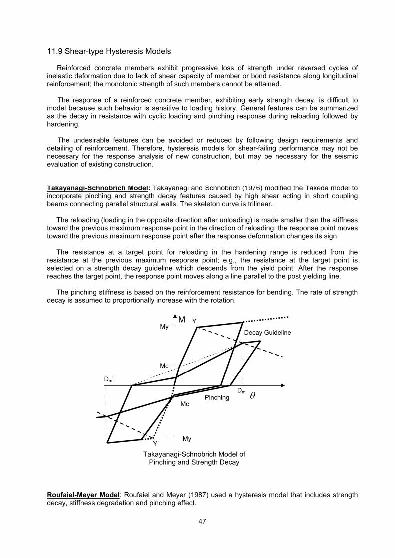
47

11.9 Shear-type Hysteresis Models

Reinforced concrete members exhibit progressive loss of strength under reversed cycles of inelastic deformation due to lack of shear capacity of member or bond resistance along longitudinal reinforcement; the monotonic strength of such members cannot be attained.

The response of a reinforced concrete member, exhibiting early strength decay, is difficult to model because such behavior is sensitive to loading history. General features can be summarized as the decay in resistance with cyclic loading and pinching response during reloading followed by hardening.

The undesirable features can be avoided or reduced by following design requirements and

detailing of reinforcement. Therefore, hysteresis models for shear-failing performance may not be necessary for the response analysis of new construction, but may be necessary for the seismic evaluation of existing construction. Takayanagi-Schnobrich Model: Takayanagi and Schnobrich (1976) modified the Takeda model to incorporate pinching and strength decay features caused by high shear acting in short coupling beams connecting parallel structural walls. The skeleton curve is trilinear.

The reloading (loading in the opposite direction after unloading) is made smaller than the stiffness toward the previous maximum response point in the direction of reloading; the response point moves toward the previous maximum response point after the response deformation changes its sign.

The resistance at a target point for reloading in the hardening range is reduced from the resistance at the previous maximum response point; e.g., the resistance at the target point is selected on a strength decay guideline which descends from the yield point. After the response reaches the target point, the response point moves along a line parallel to the post yielding line.

The pinching stiffness is based on the reinforcement resistance for bending. The rate of strength decay is assumed to proportionally increase with the rotation.

Roufaiel-Meyer Model: Roufaiel and Meyer (1987) used a hysteresis model that includes strength decay, stiffness degradation and pinching effect.

Pinching

Decay Guideline

M

Mc

Mc

My

My

θDm

Dm’

Y’

Y

Takayanagi-Schnobrich Model of

Pinching and Strength Decay

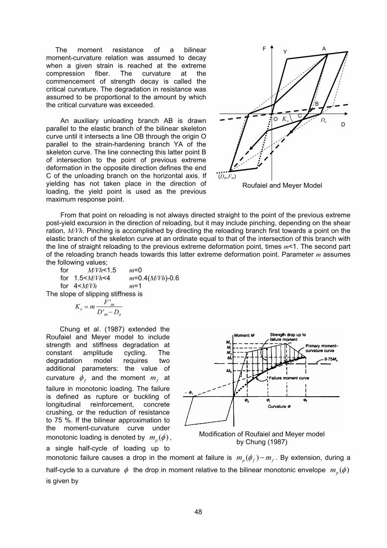
48

The moment resistance of a bilinear moment-curvature relation was assumed to decay when a given strain is reached at the extreme compression fiber. The curvature at the commencement of strength decay is called the critical curvature. The degradation in resistance was assumed to be proportional to the amount by which the critical curvature was exceeded.

An auxiliary unloading branch AB is drawn parallel to the elastic branch of the bilinear skeleton curve until it intersects a line OB through the origin O parallel to the strain-hardening branch YA of the skeleton curve. The line connecting this latter point B of intersection to the point of previous extreme deformation in the opposite direction defines the end C of the unloading branch on the horizontal axis. If yielding has not taken place in the direction of loading, the yield point is used as the previous maximum response point.

From that point on reloading is not always directed straight to the point of the previous extreme

post-yield excursion in the direction of reloading, but it may include pinching, depending on the shear ration, M/Vh. Pinching is accomplished by directing the reloading branch first towards a point on the elastic branch of the skeleton curve at an ordinate equal to that of the intersection of this branch with the line of straight reloading to the previous extreme deformation point, times m<1. The second part of the reloading branch heads towards this latter extreme deformation point. Parameter m assumes the following values;

for M/Vh<1.5 m=0 for 1.5<M/Vh<4 m=0.4(M/Vh)-0.6 for 4<M/Vh m=1

The slope of slipping stiffness is

''

ms

m o

FK mD D

=−

Chung et al. (1987) extended the

Roufaiel and Meyer model to include strength and stiffness degradation at constant amplitude cycling. The degradation model requires two additional parameters: the value of curvature fφ and the moment fm at failure in monotonic loading. The failure is defined as rupture or buckling of longitudinal reinforcement, concrete crushing, or the reduction of resistance to 75 %. If the bilinear approximation to the moment-curvature curve under monotonic loading is denoted by ( )pm φ , a single half-cycle of loading up to monotonic failure causes a drop in the moment at failure is ( )p f fm mφ − . By extension, during a

half-cycle to a curvature φ the drop in moment relative to the bilinear monotonic envelope ( )pm φ is given by

Modification of Roufaiel and Meyer model by Chung (1987)

Y F A

B

C D

O sK oD

(Dm,Fm)

Roufaiel and Meyer Model

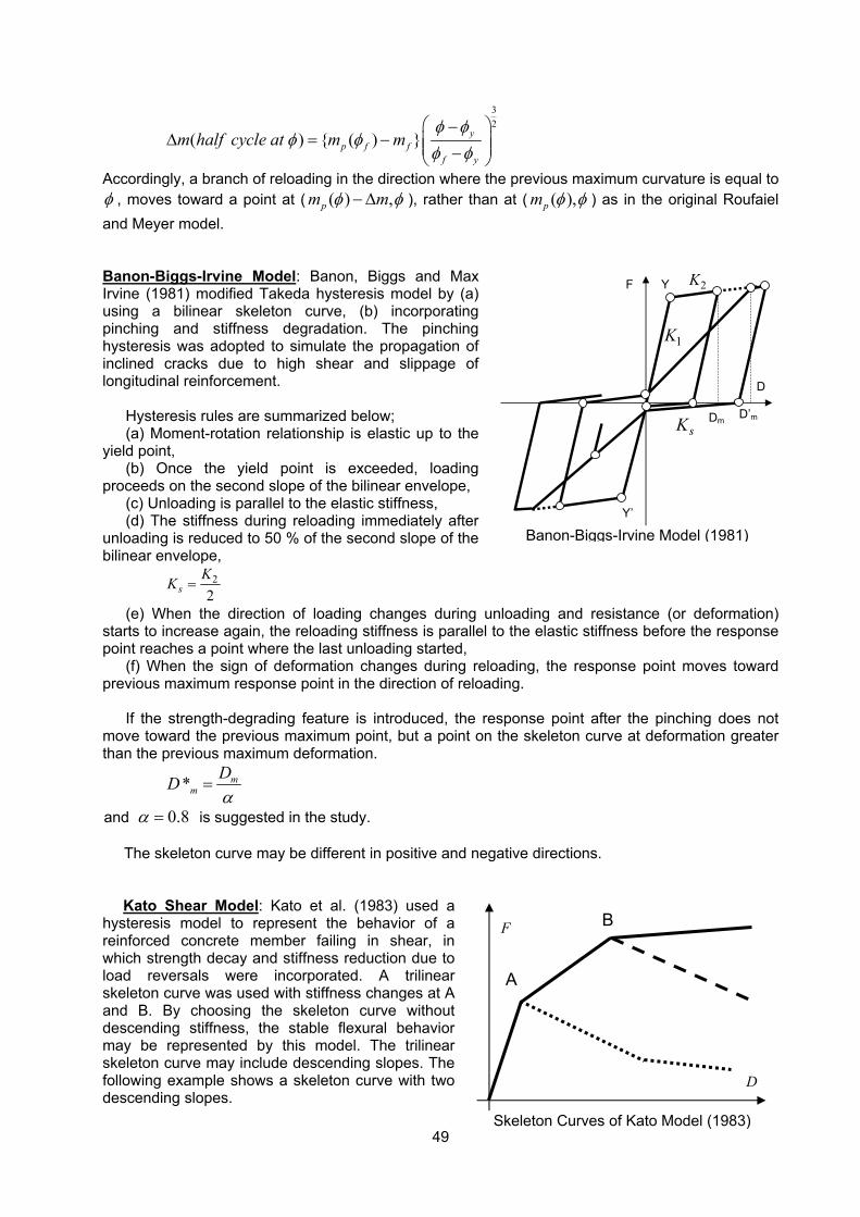
49

32

( ) { ( ) } yp f f

f y

m half cycle at m mφ φ

φ φφ φ −

∆ = − −

Accordingly, a branch of reloading in the direction where the previous maximum curvature is equal to φ , moves toward a point at ( ( ) ,pm mφ φ−∆ ), rather than at ( ( ),pm φ φ ) as in the original Roufaiel and Meyer model.

Banon-Biggs-Irvine Model: Banon, Biggs and Max Irvine (1981) modified Takeda hysteresis model by (a) using a bilinear skeleton curve, (b) incorporating pinching and stiffness degradation. The pinching hysteresis was adopted to simulate the propagation of inclined cracks due to high shear and slippage of longitudinal reinforcement.

Hysteresis rules are summarized below; (a) Moment-rotation relationship is elastic up to the

yield point, (b) Once the yield point is exceeded, loading

proceeds on the second slope of the bilinear envelope, (c) Unloading is parallel to the elastic stiffness, (d) The stiffness during reloading immediately after

unloading is reduced to 50 % of the second slope of the bilinear envelope,

2

2sKK =

(e) When the direction of loading changes during unloading and resistance (or deformation) starts to increase again, the reloading stiffness is parallel to the elastic stiffness before the response point reaches a point where the last unloading started,

(f) When the sign of deformation changes during reloading, the response point moves toward previous maximum response point in the direction of reloading.

If the strength-degrading feature is introduced, the response point after the pinching does not

move toward the previous maximum point, but a point on the skeleton curve at deformation greater than the previous maximum deformation.

* mm

DDα

=

and 0.8α = is suggested in the study.

The skeleton curve may be different in positive and negative directions.

Kato Shear Model: Kato et al. (1983) used a hysteresis model to represent the behavior of a reinforced concrete member failing in shear, in which strength decay and stiffness reduction due to load reversals were incorporated. A trilinear skeleton curve was used with stiffness changes at A and B. By choosing the skeleton curve without descending stiffness, the stable flexural behavior may be represented by this model. The trilinear skeleton curve may include descending slopes. The following example shows a skeleton curve with two descending slopes.

F

D

Y

Y’

Dm D’msK

1K

2K

Banon-Biggs-Irvine Model (1981)

D

F

A

B

Skeleton Curves of Kato Model (1983)

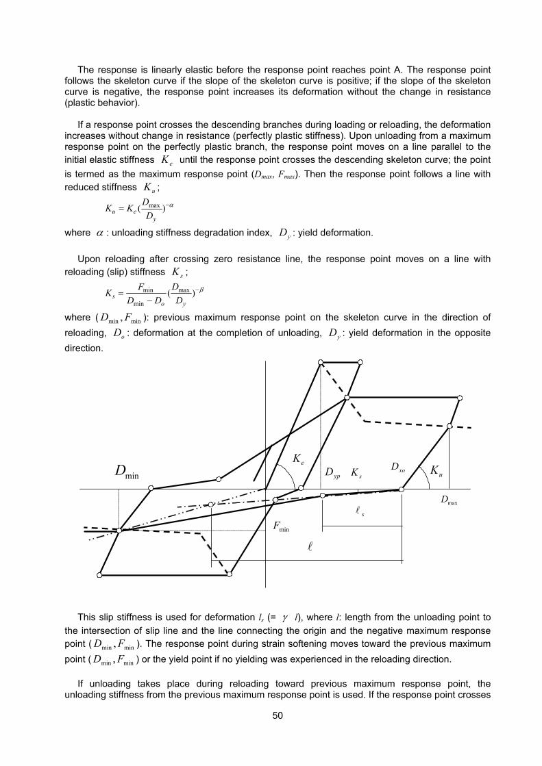
50

The response is linearly elastic before the response point reaches point A. The response point follows the skeleton curve if the slope of the skeleton curve is positive; if the slope of the skeleton curve is negative, the response point increases its deformation without the change in resistance (plastic behavior).

If a response point crosses the descending branches during loading or reloading, the deformation

increases without change in resistance (perfectly plastic stiffness). Upon unloading from a maximum response point on the perfectly plastic branch, the response point moves on a line parallel to the initial elastic stiffness eK until the response point crosses the descending skeleton curve; the point is termed as the maximum response point (Dmax, Fmax). Then the response point follows a line with reduced stiffness uK ;

max( )u ey

DK KD

α−=

where α : unloading stiffness degradation index, yD : yield deformation.

Upon reloading after crossing zero resistance line, the response point moves on a line with reloading (slip) stiffness sK ;

maxmin

min( )s

o y

DFKD D D

β−=−

where ( minmin , FD ): previous maximum response point on the skeleton curve in the direction of reloading, oD : deformation at the completion of unloading, yD : yield deformation in the opposite direction.

This slip stiffness is used for deformation ls (= γ l), where l: length from the unloading point to

the intersection of slip line and the line connecting the origin and the negative maximum response point ( minmin , FD ). The response point during strain softening moves toward the previous maximum point ( minmin , FD ) or the yield point if no yielding was experienced in the reloading direction.

If unloading takes place during reloading toward previous maximum response point, the

unloading stiffness from the previous maximum response point is used. If the response point crosses

sl

l

minF

minD

maxD

xoD ypD

eK

sK uK

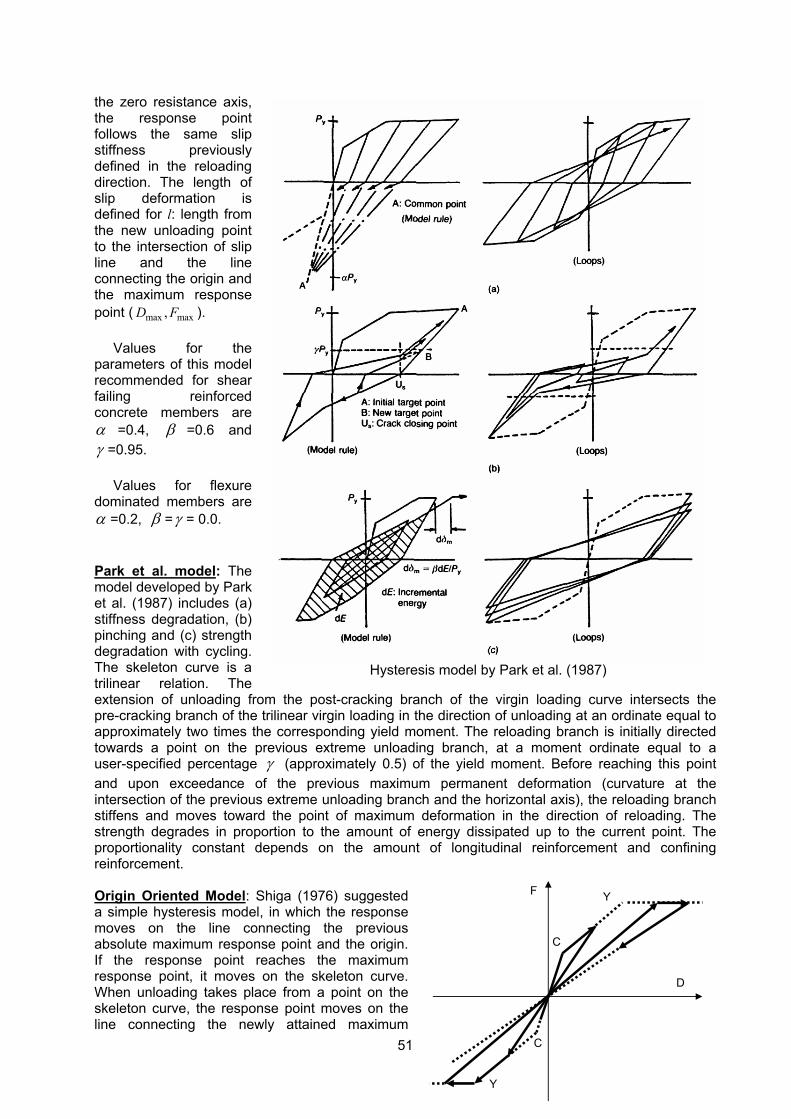
51

the zero resistance axis, the response point follows the same slip stiffness previously defined in the reloading direction. The length of slip deformation is defined for l: length from the new unloading point to the intersection of slip line and the line connecting the origin and the maximum response point ( max max,D F ).

Values for the

parameters of this model recommended for shear failing reinforced concrete members are α =0.4, β =0.6 and γ =0.95.

Values for flexure dominated members are α =0.2, β =γ = 0.0. Park et al. model: The model developed by Park et al. (1987) includes (a) stiffness degradation, (b) pinching and (c) strength degradation with cycling. The skeleton curve is a trilinear relation. The extension of unloading from the post-cracking branch of the virgin loading curve intersects the pre-cracking branch of the trilinear virgin loading in the direction of unloading at an ordinate equal to approximately two times the corresponding yield moment. The reloading branch is initially directed towards a point on the previous extreme unloading branch, at a moment ordinate equal to a user-specified percentage γ (approximately 0.5) of the yield moment. Before reaching this point and upon exceedance of the previous maximum permanent deformation (curvature at the intersection of the previous extreme unloading branch and the horizontal axis), the reloading branch stiffens and moves toward the point of maximum deformation in the direction of reloading. The strength degrades in proportion to the amount of energy dissipated up to the current point. The proportionality constant depends on the amount of longitudinal reinforcement and confining reinforcement. Origin Oriented Model: Shiga (1976) suggested a simple hysteresis model, in which the response moves on the line connecting the previous absolute maximum response point and the origin. If the response point reaches the maximum response point, it moves on the skeleton curve. When unloading takes place from a point on the skeleton curve, the response point moves on the line connecting the newly attained maximum

Hysteresis model by Park et al. (1987)

D

F

C

Y

C

Y

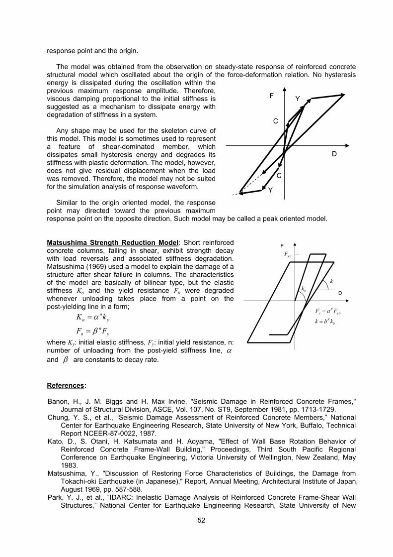
52

response point and the origin.

The model was obtained from the observation on steady-state response of reinforced concrete structural model which oscillated about the origin of the force-deformation relation. No hysteresis energy is dissipated during the oscillation within the previous maximum response amplitude. Therefore, viscous damping proportional to the initial stiffness is suggested as a mechanism to dissipate energy with degradation of stiffness in a system.

Any shape may be used for the skeleton curve of this model. This model is sometimes used to represent a feature of shear-dominated member, which dissipates small hysteresis energy and degrades its stiffness with plastic deformation. The model, however, does not give residual displacement when the load was removed. Therefore, the model may not be suited for the simulation analysis of response waveform.

Similar to the origin oriented model, the response

point may directed toward the previous maximum response point on the opposite direction. Such model may be called a peak oriented model. Matsushima Strength Reduction Model: Short reinforced concrete columns, failing in shear, exhibit strength decay with load reversals and associated stiffness degradation. Matsushima (1969) used a model to explain the damage of a structure after shear failure in columns. The characteristics of the model are basically of bilinear type, but the elastic stiffness Kn and the yield resistance Fn were degraded whenever unloading takes place from a point on the post-yielding line in a form;

y

nn

yn

n

FF

kK

β

α

=

=

where Ky: initial elastic stiffness, Fy: initial yield resistance, n: number of unloading from the post-yield stiffness line, α and β are constants to decay rate. References: Banon, H., J. M. Biggs and H. Max Irvine, "Seismic Damage in Reinforced Concrete Frames,"

Journal of Structural Division, ASCE, Vol. 107, No. ST9, September 1981, pp. 1713-1729. Chung, Y. S., et al., “Seismic Damage Assessment of Reinforced Concrete Members,” National

Center for Earthquake Engineering Research, State University of New York, Buffalo, Technical Report NCEER-87-0022, 1987.

Kato, D., S. Otani, H. Katsumata and H. Aoyama, "Effect of Wall Base Rotation Behavior of Reinforced Concrete Frame-Wall Building," Proceedings, Third South Pacific Regional Conference on Earthquake Engineering, Victoria University of Wellington, New Zealand, May 1983.

Matsushima, Y., "Discussion of Restoring Force Characteristics of Buildings, the Damage from Tokachi-oki Earthquake (in Japanese)," Report, Annual Meeting, Architectural Institute of Japan, August 1969, pp. 587-588.

Park, Y. J., et al., “IDARC: Inelastic Damage Analysis of Reinforced Concrete Frame-Shear Wall Structures,” National Center for Earthquake Engineering Research, State University of New

D

F

C

Y

C

Y

F

D0k

0

0

Ny y

N

F a F

k b k

=

=

0yF

k

53

York at Buffalo, Technical Report NCEER-87-0008, 1987. Roufaiel, M. S. L., and C. Meyer, "Analytical Modeling of Hysteretic Behavior of R/C Frames,"

Journal of Structural Division, ASCE, Vol. 113, No. 3, March 1987, pp. 429-444. Shiga, T., Vibration of Structures (in Japanese), Structural Series, Vol. 2, Kyoritsu Shuppan, 1976. Takayanagi, T., and W. C. Schnobrich, "Computed Behavior of Reinforced concrete Coupled Shear

Walls," Structural Research Series No. 434, Civil Engineering Studies, University of Illinois at Urbana-Champaign, 1976.

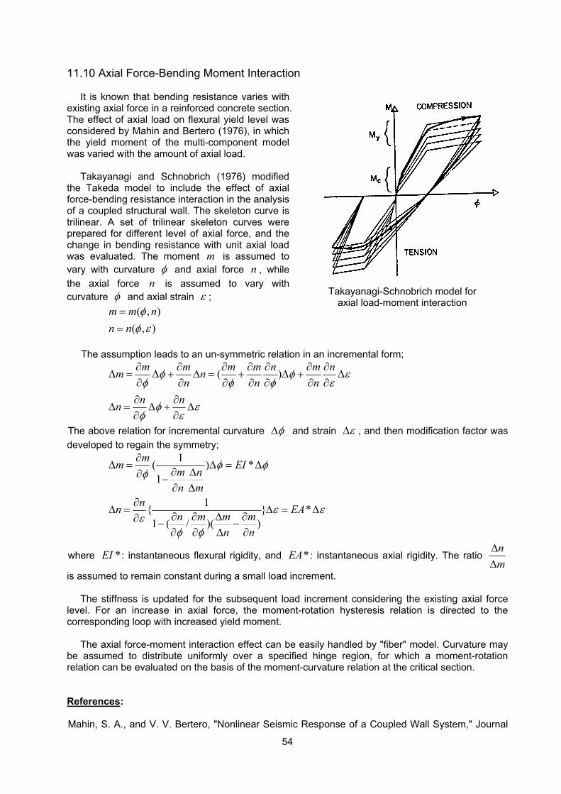
54

11.10 Axial Force-Bending Moment Interaction

It is known that bending resistance varies with existing axial force in a reinforced concrete section. The effect of axial load on flexural yield level was considered by Mahin and Bertero (1976), in which the yield moment of the multi-component model was varied with the amount of axial load.

Takayanagi and Schnobrich (1976) modified the Takeda model to include the effect of axial force-bending resistance interaction in the analysis of a coupled structural wall. The skeleton curve is trilinear. A set of trilinear skeleton curves were prepared for different level of axial force, and the change in bending resistance with unit axial load was evaluated. The moment m is assumed to vary with curvature φ and axial force n , while the axial force n is assumed to vary with curvature φ and axial strain ε ;

( , )

( , )m m nn n

φφ ε

==

The assumption leads to an un-symmetric relation in an incremental form;

( )m m m m n m nm nn n n

n nn

φ φ εφ φ φ ε

φ εφ ε

∂ ∂ ∂ ∂ ∂ ∂ ∂∆ = ∆ + ∆ = + ∆ + ∆

∂ ∂ ∂ ∂ ∂ ∂ ∂∂ ∂

∆ = ∆ + ∆∂ ∂

The above relation for incremental curvature φ∆ and strain ε∆ , and then modification factor was developed to regain the symmetry;

1( ) *1

1{ } *1 ( / )( )

mm EIm nn m

nn EAn m m mn n

φ φφ

ε εε

φ φ

∂∆ = ∆ = ∆

∂ ∆∂ −∂ ∆

∂∆ = ∆ = ∆

∂ ∂ ∆ ∂∂ − −∂ ∂ ∆ ∂

where *EI : instantaneous flexural rigidity, and *EA : instantaneous axial rigidity. The ratio nm∆∆

is assumed to remain constant during a small load increment. The stiffness is updated for the subsequent load increment considering the existing axial force

level. For an increase in axial force, the moment-rotation hysteresis relation is directed to the corresponding loop with increased yield moment.

The axial force-moment interaction effect can be easily handled by "fiber" model. Curvature may be assumed to distribute uniformly over a specified hinge region, for which a moment-rotation relation can be evaluated on the basis of the moment-curvature relation at the critical section. References: Mahin, S. A., and V. V. Bertero, "Nonlinear Seismic Response of a Coupled Wall System," Journal

Takayanagi-Schnobrich model for axial load-moment interaction

55

of Structural Division, ASCE, Vol. 102, 1976, pp. 1759-1780. Takayanagi, T., and W. C. Schnobrich, "Computed Behavior of Reinforced Concrete Coupled Shear

Walls," Structural Research Series No. 434, Civil Engineering Studies, University of Illinois at Urbana-Champaign, 1976.

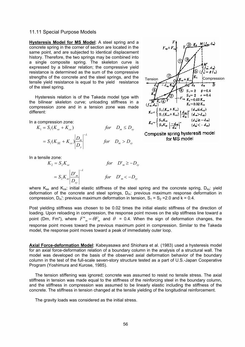
56

11.11 Special Purpose Models Hysteresis Model for MS Model: A steel spring and a concrete spring in the corner of section are located in the same point, and are subjected to identical displacement history. Therefore, the two springs may be combined into a single composite spring. The skeleton curve is expressed by a bilinear relation; the compressive yield resistance is determined as the sum of the compressive strengths of the concrete and the steel springs, and the tensile yield resistance is equal to the yield resistance of the steel spring.

Hysteresis relation is of the Takeda model type with the bilinear skeleton curve; unloading stiffness in a compression zone and in a tension zone was made different: In a compression zone:

sym

y

mceSE

symcese

DDforDDKKS

DDforKKSK

>+=

≤+=−λ

)(

)(

1

11

In a tensile zone:

sym

sy

mse

symse

DDforDDKS

DDforKSK

−<=

−≥=−

''

'

2

22

λ

where Kse and Kce: initial elastic stiffness of the steel spring and the concrete spring, Dsy: yield deformation of the concrete and steel springs, Dm: previous maximum response deformation in compression, Dm': previous maximum deformation in tension, S1 = S2 =2.0 and k = 0.4. Post yielding stiffness was chosen to be 0.02 times the initial elastic stiffness of the direction of loading. Upon reloading in compression, the response point moves on the slip stiffness line toward a point (Dm, Fm"), where mm FF θ=" and θ = 0.4. When the sign of deformation changes, the response point moves toward the previous maximum point in compression. Similar to the Takeda model, the response point moves toward a peak of immediately outer loop. Axial Force-deformation Model: Kabeyasawa and Shiohara et al. (1983) used a hysteresis model for an axial force-deformation relation of a boundary column in the analysis of a structural wall. The model was developed on the basis of the observed axial deformation behavior of the boundary column in the test of the full-scale seven-story structure tested as a part of U.S.-Japan Cooperative Program (Yoshimura and Kurose, 1985).

The tension stiffening was ignored; concrete was assumed to resist no tensile stress. The axial stiffness in tension was made equal to the stiffness of the reinforcing steel in the boundary column, and the stiffness in compression was assumed to be linearly elastic including the stiffness of the concrete. The stiffness in tension changed at the tensile yielding of the longitudinal reinforcement.

The gravity loads was considered as the initial stress.

Composite spring hysteresis model for MS model

Tension Compression

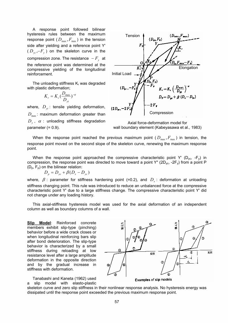
57

A response point followed bilinear hysteresis rules between the maximum response point ( maxmax , FD ) in the tension side after yielding and a reference point Y' ( yyc FD −, ) on the skeleton curve in the

compression zone. The resistance yF− at the reference point was determined at the compressive yielding of the longitudinal reinforcement.

The unloading stiffness Kr was degraded with plastic deformation;

α−= )( max

ytcr D

DKK

where, ytD : tensile yielding deformation,

maxD : maximum deformation greater than

yD , α : unloading stiffness degradation parameter (= 0.9).

When the response point reached the previous maximum point ( maxmax , FD ) in tension, the response point moved on the second slope of the skeleton curve, renewing the maximum response point.

When the response point approached the compressive characteristic point Y' (Dyc, -Fy) in compression, the response point was directed to move toward a point Y" (2Dyc, -2Fy) from a point P (Dp, Fp) on the bilinear relation: )( ycxycp DDDD −+= β

where, β : parameter for stiffness hardening point (=0.2), and xD : deformation at unloading stiffness changing point. This rule was introduced to reduce an unbalanced force at the compressive characteristic point Y' due to a large stiffness change. The compressive characteristic point Y' did not change under any loading history.

This axial-stiffness hysteresis model was used for the axial deformation of an independent column as well as boundary columns of a wall. Slip Model: Reinforced concrete members exhibit slip-type (pinching) behavior before a wide crack closes or when longitudinal reinforcing bars slip after bond deterioration. The slip-type behavior is characterized by a small stiffness during reloading at low resistance level after a large amplitude deformation in the opposite direction and by the gradual increase in stiffness with deformation.

Tanabashi and Kaneta (1962) used a slip model with elasto-plastic skeleton curve and zero slip stiffness in their nonlinear response analysis. No hysteresis energy was dissipated until the response point exceeded the previous maximum response point.

Axial force-deformation model for wall boundary element (Kabeyasawa et al., 1983)

Tension

Initial Load Elongation

Compression

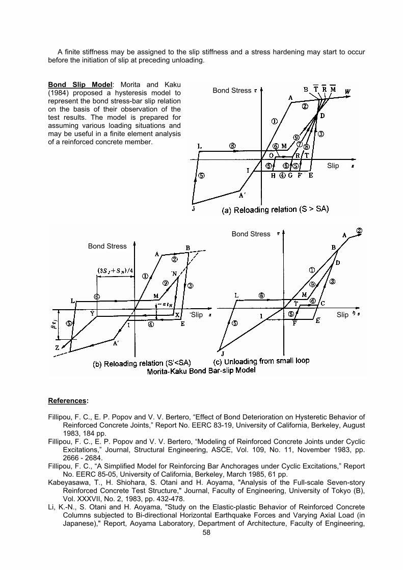
58

A finite stiffness may be assigned to the slip stiffness and a stress hardening may start to occur before the initiation of slip at preceding unloading. Bond Slip Model: Morita and Kaku (1984) proposed a hysteresis model to represent the bond stress-bar slip relation on the basis of their observation of the test results. The model is prepared for assuming various loading situations and may be useful in a finite element analysis of a reinforced concrete member.

References: Fillipou, F. C., E. P. Popov and V. V. Bertero, “Effect of Bond Deterioration on Hysteretic Behavior of

Reinforced Concrete Joints,” Report No. EERC 83-19, University of California, Berkeley, August 1983, 184 pp.

Fillipou, F. C., E. P. Popov and V. V. Bertero, “Modeling of Reinforced Concrete Joints under Cyclic Excitations,” Journal, Structural Engineering, ASCE, Vol. 109, No. 11, November 1983, pp. 2666 - 2684.

Fillipou, F. C., “A Simplified Model for Reinforcing Bar Anchorages under Cyclic Excitations,” Report No. EERC 85-05, University of California, Berkeley, March 1985, 61 pp.

Kabeyasawa, T., H. Shiohara, S. Otani and H. Aoyama, "Analysis of the Full-scale Seven-story Reinforced Concrete Test Structure," Journal, Faculty of Engineering, University of Tokyo (B), Vol. XXXVII, No. 2, 1983, pp. 432-478.

Li, K.-N., S. Otani and H. Aoyama, "Study on the Elastic-plastic Behavior of Reinforced Concrete Columns subjected to Bi-directional Horizontal Earthquake Forces and Varying Axial Load (in Japanese)," Report, Aoyama Laboratory, Department of Architecture, Faculty of Engineering,

(a) Reloading relation (S > SA)

Bond Stress

Bond Stress

Slip Slip

Bond Stress

Slip

59

University of Tokyo, March 1990. Morita, S., and T. Kaku, "Slippage of Reinforcement in Beam-column Joint of Reinforced Concrete

Frames," Proceedings, Eighth World Conference on Earthquake Engineering, San Francisco, U. S. A., Vol. 6, 1984, pp. 477-484.

Tanabashi, R., and K. Kaneta, "On the Relation between the Restoring Force Characteristics of Structures and the Pattern of Earthquake Ground Motion," Proceedings, Japan National Conference on Earthquake Engineering, November 1962, pp. 57-62.

Yoshimura, M., and Y. Kurose, "Inelastic Behavior of the Building," ACI SP-84, Earthquake Effects on Reinforced Concrete Structures, U.S.-Japan Research, American Concrete Institute, Detroit, 1985, pp. 163-202.

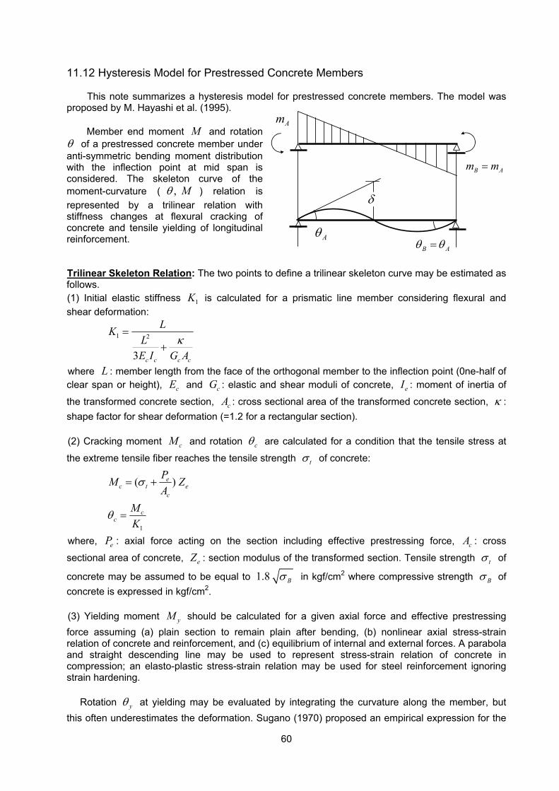
60

11.12 Hysteresis Model for Prestressed Concrete Members

This note summarizes a hysteresis model for prestressed concrete members. The model was proposed by M. Hayashi et al. (1995).

Member end moment M and rotation θ of a prestressed concrete member under anti-symmetric bending moment distribution with the inflection point at mid span is considered. The skeleton curve of the moment-curvature ( , Mθ ) relation is represented by a trilinear relation with stiffness changes at flexural cracking of concrete and tensile yielding of longitudinal reinforcement.

Trilinear Skeleton Relation: The two points to define a trilinear skeleton curve may be estimated as follows. (1) Initial elastic stiffness 1K is calculated for a prismatic line member considering flexural and shear deformation:

1 2

3 c c c c

LKLE I G A

κ=

+

where L : member length from the face of the orthogonal member to the inflection point (0ne-half of clear span or height), cE and cG : elastic and shear moduli of concrete, eI : moment of inertia of

the transformed concrete section, cA : cross sectional area of the transformed concrete section, κ : shape factor for shear deformation (=1.2 for a rectangular section). (2) Cracking moment cM and rotation cθ are calculated for a condition that the tensile stress at

the extreme tensile fiber reaches the tensile strength tσ of concrete:

1

( )ec t e

c

cc

PM ZA

MK

σ

θ

= +

=

where, eP : axial force acting on the section including effective prestressing force, cA : cross

sectional area of concrete, eZ : section modulus of the transformed section. Tensile strength tσ of

concrete may be assumed to be equal to 1.8 Bσ in kgf/cm2 where compressive strength Bσ of concrete is expressed in kgf/cm2. (3) Yielding moment yM should be calculated for a given axial force and effective prestressing force assuming (a) plain section to remain plain after bending, (b) nonlinear axial stress-strain relation of concrete and reinforcement, and (c) equilibrium of internal and external forces. A parabola and straight descending line may be used to represent stress-strain relation of concrete in compression; an elasto-plastic stress-strain relation may be used for steel reinforcement ignoring strain hardening.

Rotation yθ at yielding may be evaluated by integrating the curvature along the member, but this often underestimates the deformation. Sugano (1970) proposed an empirical expression for the

Am

B Am m=

δ

AθB Aθ θ=

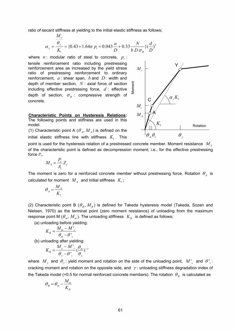
61

ratio of secant stiffness at yielding to the initial elastic stiffness as follows;

2

1

{0.43 1.64 0.043 0.33 }( )

y

yy t

B

Ma N dn p

K D b D Dθ

ασ

= = + + +

where n : modular ratio of steel to concrete, tp : tensile reinforcement ratio including prestressing reinforcement area as increased by the yield stress ratio of prestressing reinforcement to ordinary reinforcement, a : shear span, b and D : width and depth of member section, N : axial force of section including effective prestressing force, d : effective depth of section, Bσ : compressive strength of concrete. Characteristic Points on Hysteresis Relations: The following points and stiffness are used in this model. (1) Characteristic point A ( ,A AMθ ) is defined on the initial elastic stiffness line with stiffness 1K . This point is used for the hysteresis relation of a prestressed concrete member. Moment resistance AM of the characteristic point is defined as decompression moment; i.e., for the effective prestressing force Pe,

eA e

c

PM ZA

=

The moment is zero for a reinforced concrete member without prestressing force. Rotation Aθ is calculated for moment AM and initial stiffness 1K ;

1

AA

MK

θ =

(2) Characteristic point B ( ,B BMθ ) is defined for Takeda hysteresis model (Takeda, Sozen and Nielsen, 1970) as the terminal point (zero moment resistance) of unloading from the maximum response point M ( ,m mMθ ). The unloading stiffness BK is defined as follows;

(a) unloading before yielding:

'

'm c

Bm c

M MKθ θ

−=

−

(b) unloading after yielding:

'

( )'

y c mB

y c y

M MK γθ

θ θ θ−−

=−

where yM and yθ : yield moment and rotation on the side of the unloading point, 'cM and 'cθ : cracking moment and rotation on the opposite side, and γ : unloading stiffness degradation index of the Takeda model (=0.5 for normal reinforced concrete members). The rotation Bθ is calculated as

mB m

B

MK

θ θ= −

C

Y

yθ cθ

cM

yM

Rotation

Mom

ent

1K

1y Kα

A

Aθ

AM

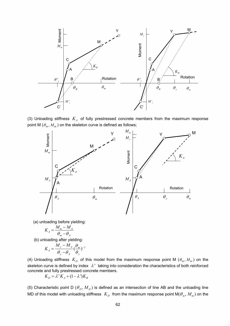
62

C

Y

Rotation

Mom

ent

A

C’ 'cM

'cθ

C

Y

yθ

yM

Rotation

Mom

ent

A

C’'cM

'cθ

MmM

mθ

B

Bθ

BK

B

BK

mθBθ

M

(3) Unloading stiffness AK of fully prestressed concrete members from the maximum response point M ( ,m mMθ ) on the skeleton curve is defined as follows;

C

Y

Rotation

Mom

ent

A

Aθ

AM

M mM

AK C

Y

yθ

yM

Rotation

Mom

ent

A

Aθ

AM

MmM

mθ

AK

mθ

(a) unloading before yielding:

m AA

m A

M MKθ θ

−=

−

(b) unloading after yielding:

( )y A mA

y A y

M MK γθ

θ θ θ−−

=−

(4) Unloading stiffness DK of this model from the maximum response point M ( ,m mMθ ) on the skeleton curve is defined by index 'λ taking into consideration the characteristics of both reinforced concrete and fully prestressed concrete members. ' (1 ')D A BK K Kλ λ= + − (5) Characteristic point D ( ,D DMθ ) is defined as an intersection of line AB and the unloading line MD of this model with unloading stiffness DK from the maximum response point M( ,m mMθ ) on the

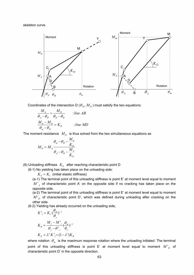
63

skeleton curve.

Coordinates of the intersection D ( ,D DMθ ) must satisfy the two equations;

:

:

A D

A B D B

m DD

m D

M M line AB

M M K line MD

θ θ θ θ

θ θ

=− −−

=−

The moment resistance DM is thus solved from the two simultaneous equations as

mm B

DD A

AA B

D

MKM M MK

θ θ

θ θ

− −=

− −

(6) Unloading stiffness EK after reaching characteristic point D

(6-1) No yielding has taken place on the unloading side: 1EK K= (initial elastic stiffness)

(a-1) The terminal point of this unloading stiffness is point E’ at moment level equal to moment 'AM of characteristic point A’ on the opposite side if no cracking has taken place on the

opposite side. (a-2) The terminal point of this unloading stiffness is point E’ at moment level equal to moment

'DM of characteristic point D’, which was defined during unloading after cracking on the other side.

(6-2) Yielding has already occurred on the unloading side,

1 1

1

' ( )

'( )

'

' ' (1 ')

m

y

y c mB

y c y

E B

K K

M MK

K K K

γ

γ

θθ

θθ θ θ

λ λ

−

−

=

−=

−

= + −

where rotation mθ is the maximum response rotation where the unloading initiated. The terminal

point of this unloading stiffness is point E’ at moment level equal to moment 'DM of characteristic point D’ in the opposite direction.

DK

Rotation

Moment Y

M

C

A D

B

mM

AM

mθBθ Aθ

Rotation

Moment

C

Y M

DK

AD

B

mM

AM

Aθ yθ mθ

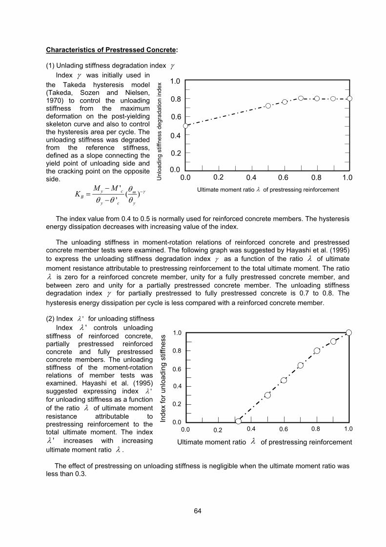
64

Characteristics of Prestressed Concrete: (1) Unlading stiffness degradation index γ

Index γ was initially used in the Takeda hysteresis model (Takeda, Sozen and Nielsen, 1970) to control the unloading stiffness from the maximum deformation on the post-yielding skeleton curve and also to control the hysteresis area per cycle. The unloading stiffness was degraded from the reference stiffness, defined as a slope connecting the yield point of unloading side and the cracking point on the opposite side.

'

( )'

y c mB

y c y

M MK γθ

θ θ θ−−

=−

The index value from 0.4 to 0.5 is normally used for reinforced concrete members. The hysteresis

energy dissipation decreases with increasing value of the index. The unloading stiffness in moment-rotation relations of reinforced concrete and prestressed

concrete member tests were examined. The following graph was suggested by Hayashi et al. (1995) to express the unloading stiffness degradation index γ as a function of the ratio λ of ultimate moment resistance attributable to prestressing reinforcement to the total ultimate moment. The ratio λ is zero for a reinforced concrete member, unity for a fully prestressed concrete member, and between zero and unity for a partially prestressed concrete member. The unloading stiffness degradation index γ for partially prestressed to fully prestressed concrete is 0.7 to 0.8. The hysteresis energy dissipation per cycle is less compared with a reinforced concrete member. (2) Index 'λ for unloading stiffness

Index 'λ controls unloading stiffness of reinforced concrete, partially prestressed reinforced concrete and fully prestressed concrete members. The unloading stiffness of the moment-rotation relations of member tests was examined. Hayashi et al. (1995) suggested expressing index 'λ for unloading stiffness as a function of the ratio λ of ultimate moment resistance attributable to prestressing reinforcement to the total ultimate moment. The index

'λ increases with increasing ultimate moment ratio λ .

The effect of prestressing on unloading stiffness is negligible when the ultimate moment ratio was less than 0.3.

0.0 0.2 0.4 0.6 0.8 1.0

1.0

0.0

0.2

0.4

0.6

0.8

Unl

oadi

ng s

tiffn

ess

degr

adat

ion

inde

x

Ultimate moment ratio of prestressing reinforcement λ

Inde

x fo

r unl

oadi

ng s

tiffn

ess

0.0 0.2 0.4 0.6 0.8 1.00.0

0.2

0.4

0.6

0.8

1.0

Ultimate moment ratio λ of prestressing reinforcement

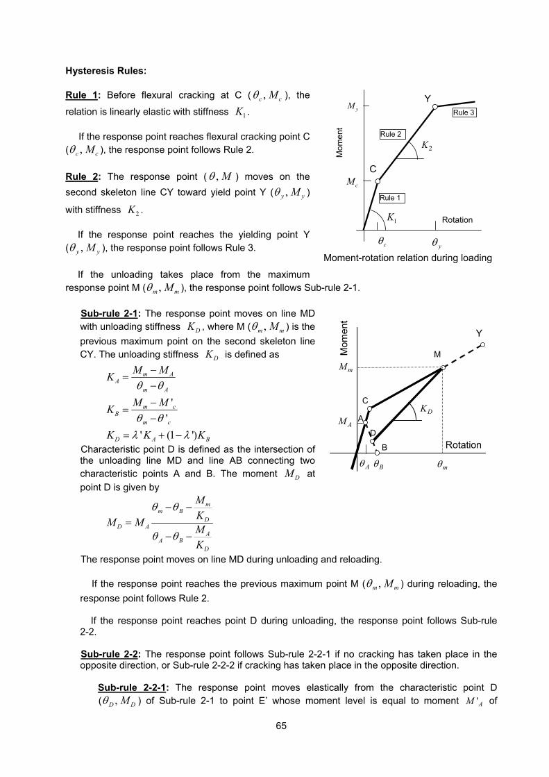
65

Hysteresis Rules: Rule 1: Before flexural cracking at C ( ,c cMθ ), the

relation is linearly elastic with stiffness 1K .

If the response point reaches flexural cracking point C ( ,c cMθ ), the response point follows Rule 2. Rule 2: The response point ( , Mθ ) moves on the second skeleton line CY toward yield point Y ( ,y yMθ )

with stiffness 2K .

If the response point reaches the yielding point Y ( ,y yMθ ), the response point follows Rule 3.

If the unloading takes place from the maximum

response point M ( ,m mMθ ), the response point follows Sub-rule 2-1. Sub-rule 2-1: The response point moves on line MD with unloading stiffness DK , where M ( ,m mMθ ) is the previous maximum point on the second skeleton line CY. The unloading stiffness DK is defined as

'

'' (1 ')

m AA

m A

m cB

m c

D A B

M MK

M MK

K K K

θ θ

θ θλ λ

−=

−−

=−

= + −

Characteristic point D is defined as the intersection of the unloading line MD and line AB connecting two characteristic points A and B. The moment DM at point D is given by

mm B

DD A

AA B

D

MKM M MK

θ θ

θ θ

− −=

− −

The response point moves on line MD during unloading and reloading. If the response point reaches the previous maximum point M ( ,m mMθ ) during reloading, the

response point follows Rule 2.

If the response point reaches point D during unloading, the response point follows Sub-rule 2-2. Sub-rule 2-2: The response point follows Sub-rule 2-2-1 if no cracking has taken place in the opposite direction, or Sub-rule 2-2-2 if cracking has taken place in the opposite direction.

Sub-rule 2-2-1: The response point moves elastically from the characteristic point D ( ,D DMθ ) of Sub-rule 2-1 to point E’ whose moment level is equal to moment 'AM of

C

Y

yθ cθ

cM

yM

Rotation

Mom

ent

1K

2K

Rule 1

Rule 2

Rule 3

Moment-rotation relation during loading

C

Rotation

AAM

M

mθ

B

DK

Y

D

Mom

ent

Bθ

mM

Aθ

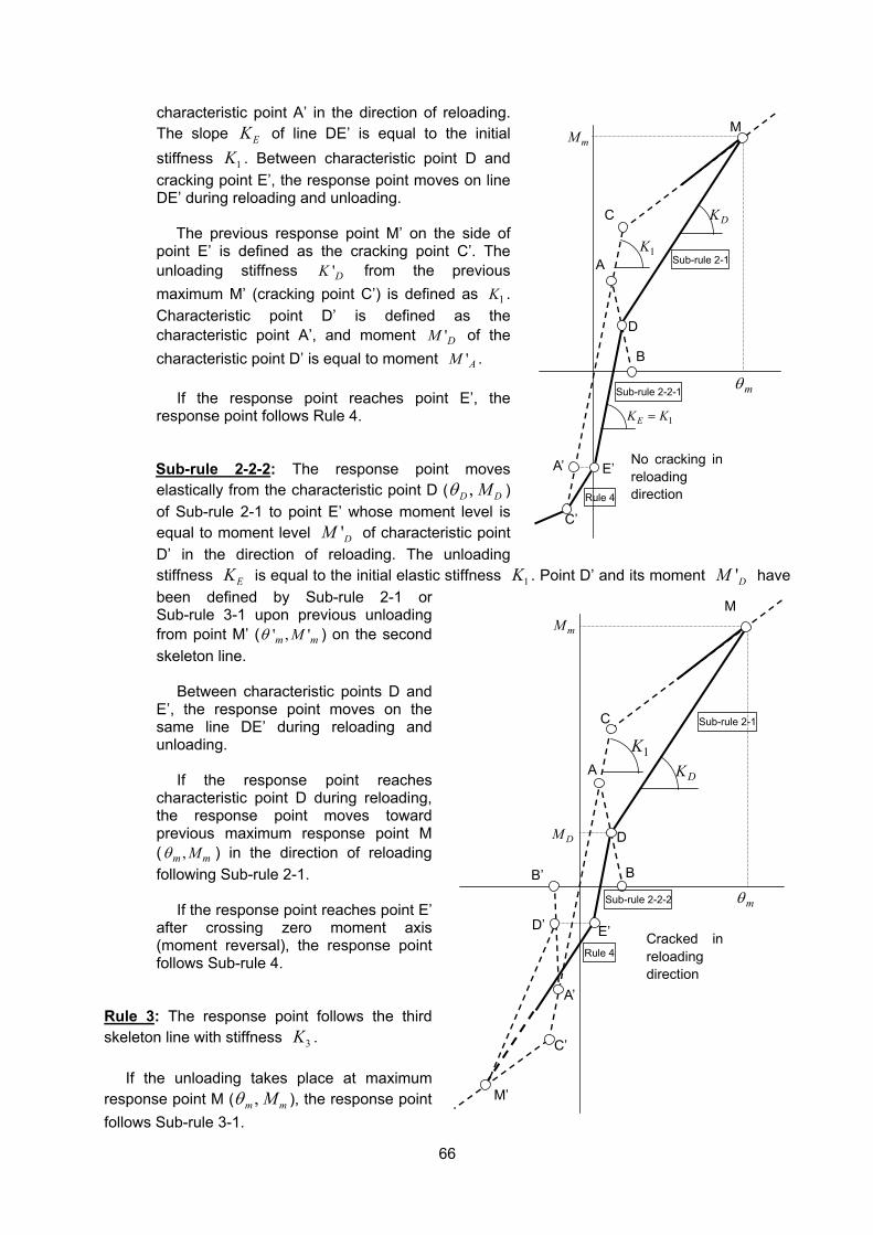
66

characteristic point A’ in the direction of reloading. The slope EK of line DE’ is equal to the initial stiffness 1K . Between characteristic point D and cracking point E’, the response point moves on line DE’ during reloading and unloading.

The previous response point M’ on the side of point E’ is defined as the cracking point C’. The unloading stiffness 'DK from the previous maximum M’ (cracking point C’) is defined as 1K . Characteristic point D’ is defined as the characteristic point A’, and moment 'DM of the characteristic point D’ is equal to moment 'AM .

If the response point reaches point E’, the response point follows Rule 4. Sub-rule 2-2-2: The response point moves elastically from the characteristic point D ( ,D DMθ ) of Sub-rule 2-1 to point E’ whose moment level is equal to moment level 'DM of characteristic point D’ in the direction of reloading. The unloading stiffness EK is equal to the initial elastic stiffness 1K . Point D’ and its moment 'DM have been defined by Sub-rule 2-1 or Sub-rule 3-1 upon previous unloading from point M’ ( ' , 'm mMθ ) on the second skeleton line.

Between characteristic points D and E’, the response point moves on the same line DE’ during reloading and unloading.

If the response point reaches

characteristic point D during reloading, the response point moves toward previous maximum response point M ( ,m mMθ ) in the direction of reloading following Sub-rule 2-1.

If the response point reaches point E’ after crossing zero moment axis (moment reversal), the response point follows Sub-rule 4.

Rule 3: The response point follows the third skeleton line with stiffness 3K .

If the unloading takes place at maximum response point M ( ,m mMθ ), the response point follows Sub-rule 3-1.

1K A

B

C

D

E’A’

C’

1EK K=

mθ

mM

No cracking in reloading direction

M

DK

Sub-rule 2-1

Sub-rule 2-2-1

Rule 4

1K

DK A

B

C

D

E’

A’

B’

C’

M’

D’Cracked in reloading direction

DM

mM

mθ

M

Sub-rule 2-1

Sub-rule 2-2-2

Rule 4

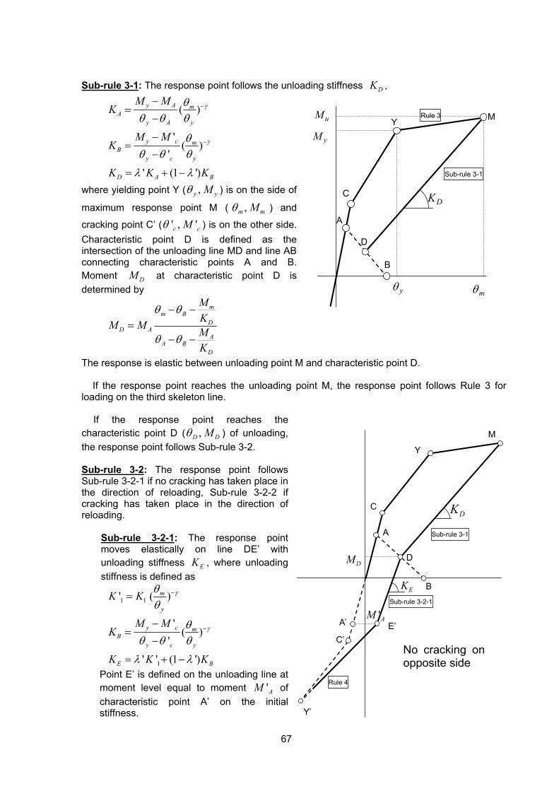
67

Sub-rule 3-1: The response point follows the unloading stiffness DK ,

( )

'( )

'

' (1 ')

y A mA

y A y

y c mB

y c y

D A B

M MK

M MK

K K K

γ

γ

θθ θ θ

θθ θ θ

λ λ

−

−

−=

−

−=

−

= + −

where yielding point Y ( ,y yMθ ) is on the side of

maximum response point M ( ,m mMθ ) and

cracking point C’ ( ' , 'c cMθ ) is on the other side. Characteristic point D is defined as the intersection of the unloading line MD and line AB connecting characteristic points A and B. Moment DM at characteristic point D is determined by

mm B

DD A

AA B

D

MKM M MK

θ θ

θ θ

− −=

− −

The response is elastic between unloading point M and characteristic point D.

If the response point reaches the unloading point M, the response point follows Rule 3 for loading on the third skeleton line.

If the response point reaches the characteristic point D ( ,D DMθ ) of unloading, the response point follows Sub-rule 3-2. Sub-rule 3-2: The response point follows Sub-rule 3-2-1 if no cracking has taken place in the direction of reloading, Sub-rule 3-2-2 if cracking has taken place in the direction of reloading.

Sub-rule 3-2-1: The response point moves elastically on line DE’ with unloading stiffness EK , where unloading stiffness is defined as

1 1

1

' ( )

'( )

'

' ' (1 ')

m

y

y c mB

y c y

E B

K K

M MK

K K K

γ

γ

θθ

θθ θ θ

λ λ

−

−

=

−=

−

= + −

Point E’ is defined on the unloading line at moment level equal to moment 'AM of characteristic point A’ on the initial stiffness.

A

C

Y

M

B

'AM

Y’

C’

D DM

DK

E’

EK

A’

No cracking on opposite side

Sub-rule 3-1

Sub-rule 3-2-1

Rule 4

C

Y M

A

D

B

DK

mθyθ

yM

uM

Sub-rule 3-1

Rule 3

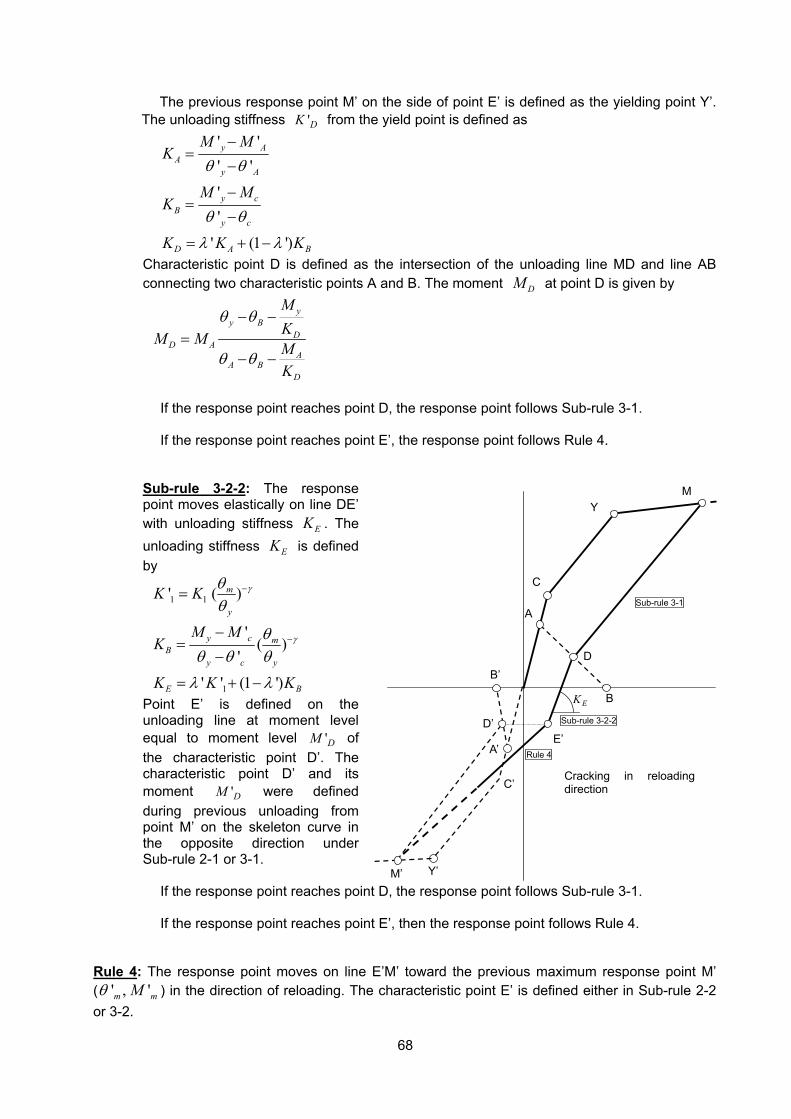
68

The previous response point M’ on the side of point E’ is defined as the yielding point Y’. The unloading stiffness 'DK from the yield point is defined as

' '' '

''

' (1 ')

y AA

y A

y cB

y c

D A B

M MK

M MK

K K K

θ θ

θ θ

λ λ

−=

−

−=

−

= + −

Characteristic point D is defined as the intersection of the unloading line MD and line AB connecting two characteristic points A and B. The moment DM at point D is given by

yy B

DD A

AA B

D

MKM M MK

θ θ

θ θ

− −=

− −

If the response point reaches point D, the response point follows Sub-rule 3-1. If the response point reaches point E’, the response point follows Rule 4.

Sub-rule 3-2-2: The response point moves elastically on line DE’ with unloading stiffness EK . The unloading stiffness EK is defined by

1 1

1

' ( )

'( )

'

' ' (1 ')

m

y

y c mB

y c y

E B

K K

M MK

K K K

γ

γ

θθ

θθ θ θ

λ λ

−

−

=

−=

−

= + −

Point E’ is defined on the unloading line at moment level equal to moment level 'DM of the characteristic point D’. The characteristic point D’ and its moment 'DM were defined during previous unloading from point M’ on the skeleton curve in the opposite direction under Sub-rule 2-1 or 3-1.

If the response point reaches point D, the response point follows Sub-rule 3-1. If the response point reaches point E’, then the response point follows Rule 4.

Rule 4: The response point moves on line E’M’ toward the previous maximum response point M’ ( ' , 'm mMθ ) in the direction of reloading. The characteristic point E’ is defined either in Sub-rule 2-2 or 3-2.

A

B

C

D

Y M

C’

A’

Y’M’

B’

D’E’

EK

Cracking in reloading direction

Sub-rule 3-1

Sub-rule 3-2-2

Rule 4

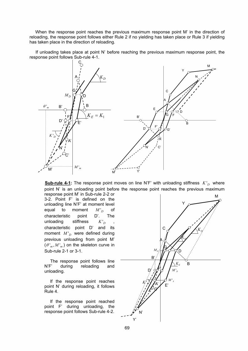
69

When the response point reaches the previous maximum response point M’ in the direction of reloading, the response point follows either Rule 2 if no yielding has taken place or Rule 3 if yielding has taken place in the direction of reloading.

If unloading takes place at point N’ before reaching the previous maximum response point, the

response point follows Sub-rule 4-1.

1EK K=

DKA

B

C

D

E’

A’

B’

C’

M’

D’

DM

F’

G

N’

'DK

'mM

'mθ

A

B

C

D

Y M

C’

A’

B’

D’

Y’M’

G’

E

N

F

N’

F’

G

Sub-rule 4-1: The response point moves on line N’F’ with unloading stiffness 'DK where point N’ is an unloading point before the response point reaches the previous maximum response point M’ in Sub-rule 2-2 or 3-2. Point F’ is defined on the unloading line N’F’ at moment level equal to moment 'DM of characteristic point D’. The unloading stiffness 'DK , characteristic point D’ and its moment 'DM were defined during previous unloading from point M’ ( ' , 'm mMθ ) on the skeleton curve in Sub-rule 2-1 or 3-1.

The response point follows line N’F’ during reloading and unloading.

If the response point reaches point N’ during reloading, it follows Rule 4.

If the response point reached

point F’ during unloading, the response point follows Sub-rule 4-2.

A

C

Y

M

B

'AM

'DM

B’

Y’

C’

D DM

DK

E’

EK

N’

A’'DK

D’

DK

F’

G

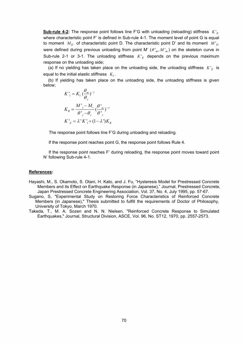
70

Sub-rule 4-2: The response point follows line F’G with unloading (reloading) stiffness 'EK where characteristic point F’ is defined in Sub-rule 4-1. The moment level of point G is equal to moment DM of characteristic point D. The characteristic point D’ and its moment 'DM were defined during previous unloading from point M’ ( ' , 'm mMθ ) on the skeleton curve in Sub-rule 2-1 or 3-1. The unloading stiffness 'EK depends on the previous maximum response on the unloading side;

(a) If no yielding has taken place on the unloading side, the unloading stiffness 'EK is equal to the initial elastic stiffness 1K .

(b) If yielding has taken place on the unloading side, the unloading stiffness is given below;

1 1

1

' ( )

' '( )' '

' ' ' (1 ')

m

y

y c mB

y c y

E B

K K

M MK

K K K

γ

γ

θθ

θθ θ θ

λ λ

−

−

=

−=

−

= + −

The response point follows line F’G during unloading and reloading.

If the response point reaches point G, the response point follows Rule 4.

If the response point reaches F’ during reloading, the response point moves toward point

N’ following Sub-rule 4-1.

References: Hayashi, M., S. Okamoto, S. Otani, H. Kato, and J. Fu, “Hysteresis Model for Prestressed Concrete

Members and its Effect on Earthquake Response (in Japanese),” Journal, Prestressed Concrete, Japan Prestressed Concrete Engineering Association, Vol. 37, No. 4, July 1995, pp. 57-67.

Sugano, S, "Experimental Study on Restoring Force Characteristics of Reinforced Concrete Members (in Japanese)," Thesis submitted to fulfill the requirements of Doctor of Philosophy, University of Tokyo, March 1970.

Takeda, T., M. A. Sozen and N. N. Nielsen, "Reinforced Concrete Response to Simulated Earthquakes," Journal, Structural Division, ASCE, Vol. 96, No. ST12, 1970, pp. 2557-2573.

71

Home Assignment No. 6

2002-03-11 Otani, S.

Displacement history is given below; (1) D= 0.0 (2) D= 2.0 Dy (3) D=-2.0 Dy (4) D= Dy (5) D=-0.5 Dy (6) D= 4.0 Dy (7) D= -2.0 Dy (8) D= 4.0 Dy where Fy=1.0, Dy=1.0. The skeleton curve is elasto-plastic. Draw resistance-deformation (F-D) relation for the two hysteresis models; (1) Clough Model (no unloading stiffness degradation) (2) Pivot hysteresis model ( 2.0α = , 0.5β = )

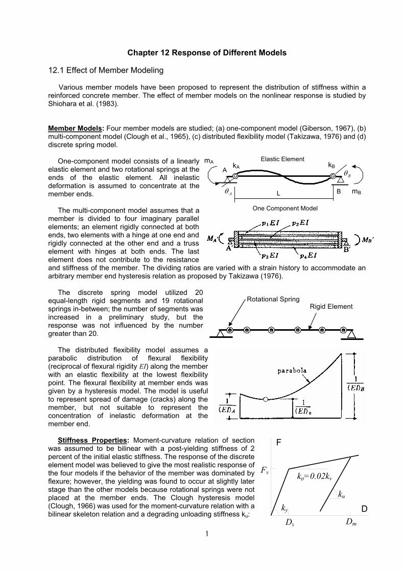
1

Chapter 12 Response of Different Models 12.1 Effect of Member Modeling

Various member models have been proposed to represent the distribution of stiffness within a reinforced concrete member. The effect of member models on the nonlinear response is studied by Shiohara et al. (1983). Member Models: Four member models are studied; (a) one-component model (Giberson, 1967), (b) multi-component model (Clough et al., 1965), (c) distributed flexibility model (Takizawa, 1976) and (d) discrete spring model.

One-component model consists of a linearly

elastic element and two rotational springs at the ends of the elastic element. All inelastic deformation is assumed to concentrate at the member ends.

The multi-component model assumes that a

member is divided to four imaginary parallel elements; an element rigidly connected at both ends, two elements with a hinge at one end and rigidly connected at the other end and a truss element with hinges at both ends. The last element does not contribute to the resistance and stiffness of the member. The dividing ratios are varied with a strain history to accommodate an arbitrary member end hysteresis relation as proposed by Takizawa (1976).

The discrete spring model utilized 20

equal-length rigid segments and 19 rotational springs in-between; the number of segments was increased in a preliminary study, but the response was not influenced by the number greater than 20.

The distributed flexibility model assumes a

parabolic distribution of flexural flexibility (reciprocal of flexural rigidity EI) along the member with an elastic flexibility at the lowest flexibility point. The flexural flexibility at member ends was given by a hysteresis model. The model is useful to represent spread of damage (cracks) along the member, but not suitable to represent the concentration of inelastic deformation at the member end.

Stiffness Properties: Moment-curvature relation of section

was assumed to be bilinear with a post-yielding stiffness of 2 percent of the initial elastic stiffness. The response of the discrete element model was believed to give the most realistic response of the four models if the behavior of the member was dominated by flexure; however, the yielding was found to occur at slightly later stage than the other models because rotational springs were not placed at the member ends. The Clough hysteresis model (Clough, 1966) was used for the moment-curvature relation with a bilinear skeleton relation and a degrading unloading stiffness ku:

ky

kp=0.02ky

ku

Dy Dm

Fy

F

D

Rotational Spring Rigid Element

One Component Model

mA

mBAθ

A

B

kA kBElastic Element

Bθ

L

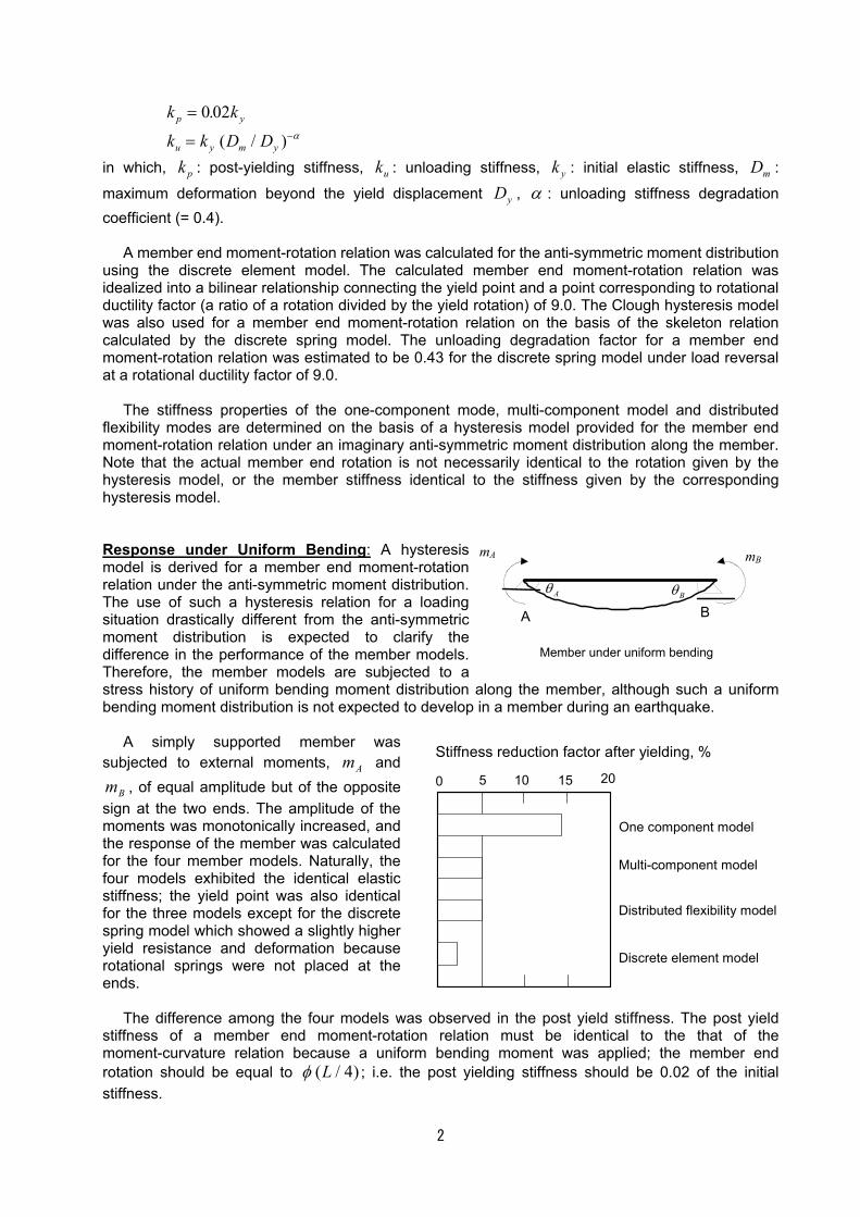
2

k kp y= 0 02.

k k D Du y m y= −( / ) α

in which, kp : post-yielding stiffness, ku : unloading stiffness, k y : initial elastic stiffness, Dm :

maximum deformation beyond the yield displacement Dy , α : unloading stiffness degradation coefficient (= 0.4).

A member end moment-rotation relation was calculated for the anti-symmetric moment distribution

using the discrete element model. The calculated member end moment-rotation relation was idealized into a bilinear relationship connecting the yield point and a point corresponding to rotational ductility factor (a ratio of a rotation divided by the yield rotation) of 9.0. The Clough hysteresis model was also used for a member end moment-rotation relation on the basis of the skeleton relation calculated by the discrete spring model. The unloading degradation factor for a member end moment-rotation relation was estimated to be 0.43 for the discrete spring model under load reversal at a rotational ductility factor of 9.0.

The stiffness properties of the one-component mode, multi-component model and distributed

flexibility modes are determined on the basis of a hysteresis model provided for the member end moment-rotation relation under an imaginary anti-symmetric moment distribution along the member. Note that the actual member end rotation is not necessarily identical to the rotation given by the hysteresis model, or the member stiffness identical to the stiffness given by the corresponding hysteresis model.

Response under Uniform Bending: A hysteresis model is derived for a member end moment-rotation relation under the anti-symmetric moment distribution. The use of such a hysteresis relation for a loading situation drastically different from the anti-symmetric moment distribution is expected to clarify the difference in the performance of the member models. Therefore, the member models are subjected to a stress history of uniform bending moment distribution along the member, although such a uniform bending moment distribution is not expected to develop in a member during an earthquake.

A simply supported member was subjected to external moments, Am and

Bm , of equal amplitude but of the opposite sign at the two ends. The amplitude of the moments was monotonically increased, and the response of the member was calculated for the four member models. Naturally, the four models exhibited the identical elastic stiffness; the yield point was also identical for the three models except for the discrete spring model which showed a slightly higher yield resistance and deformation because rotational springs were not placed at the ends.

The difference among the four models was observed in the post yield stiffness. The post yield stiffness of a member end moment-rotation relation must be identical to the that of the moment-curvature relation because a uniform bending moment was applied; the member end rotation should be equal to φ ( / )L 4 ; i.e. the post yielding stiffness should be 0.02 of the initial stiffness.

A B

mA mB

Aθ Bθ

Member under uniform bending

0 5 10 15 20

Stiffness reduction factor after yielding, %

One component model

Multi-component model

Distributed flexibility model

Discrete element model

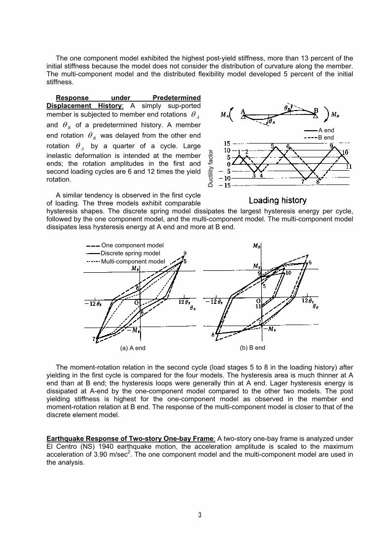
3

The one component model exhibited the highest post-yield stiffness, more than 13 percent of the

initial stiffness because the model does not consider the distribution of curvature along the member. The multi-component model and the distributed flexibility model developed 5 percent of the initial stiffness.

Response under Predetermined Displacement History: A simply sup-ported member is subjected to member end rotations θ A and θ B of a predetermined history. A member end rotation θ B was delayed from the other end rotation θ A by a quarter of a cycle. Large inelastic deformation is intended at the member ends; the rotation amplitudes in the first and second loading cycles are 6 and 12 times the yield rotation.

A similar tendency is observed in the first cycle

of loading. The three models exhibit comparable hysteresis shapes. The discrete spring model dissipates the largest hysteresis energy per cycle, followed by the one component model, and the multi-component model. The multi-component model dissipates less hysteresis energy at A end and more at B end.

One component modelDiscrete spring model Multi-component model

(a) A end (b) B end

The moment-rotation relation in the second cycle (load stages 5 to 8 in the loading history) after

yielding in the first cycle is compared for the four models. The hysteresis area is much thinner at A end than at B end; the hysteresis loops were generally thin at A end. Lager hysteresis energy is dissipated at A-end by the one-component model compared to the other two models. The post yielding stiffness is highest for the one-component model as observed in the member end moment-rotation relation at B end. The response of the multi-component model is closer to that of the discrete element model.

Earthquake Response of Two-story One-bay Frame: A two-story one-bay frame is analyzed under El Centro (NS) 1940 earthquake motion, the acceleration amplitude is scaled to the maximum acceleration of 3.90 m/sec2. The one component model and the multi-component model are used in the analysis.

A endB end

Duc

tility

fact

or

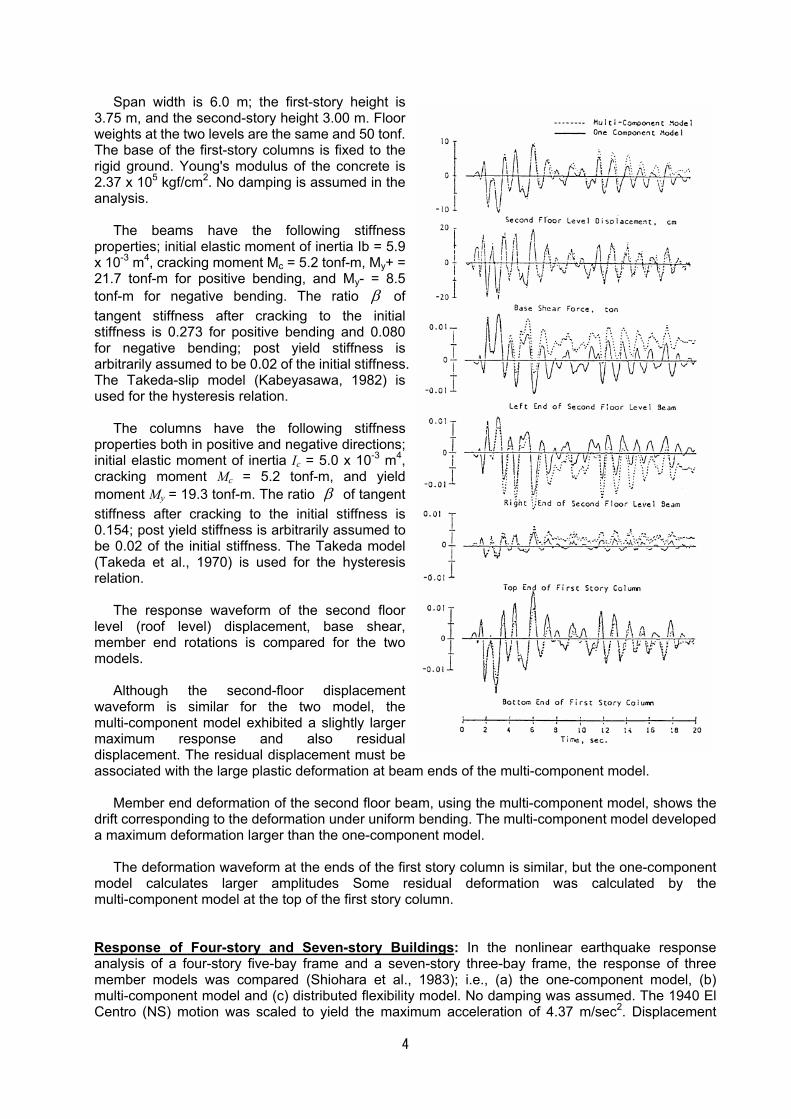
4

Span width is 6.0 m; the first-story height is 3.75 m, and the second-story height 3.00 m. Floor weights at the two levels are the same and 50 tonf. The base of the first-story columns is fixed to the rigid ground. Young's modulus of the concrete is 2.37 x 105 kgf/cm2. No damping is assumed in the analysis.

The beams have the following stiffness properties; initial elastic moment of inertia Ib = 5.9 x 10-3 m4, cracking moment Mc = 5.2 tonf-m, My+ = 21.7 tonf-m for positive bending, and My- = 8.5 tonf-m for negative bending. The ratio β of tangent stiffness after cracking to the initial stiffness is 0.273 for positive bending and 0.080 for negative bending; post yield stiffness is arbitrarily assumed to be 0.02 of the initial stiffness. The Takeda-slip model (Kabeyasawa, 1982) is used for the hysteresis relation.

The columns have the following stiffness

properties both in positive and negative directions; initial elastic moment of inertia Ic = 5.0 x 10-3 m4, cracking moment Mc = 5.2 tonf-m, and yield moment My = 19.3 tonf-m. The ratio β of tangent stiffness after cracking to the initial stiffness is 0.154; post yield stiffness is arbitrarily assumed to be 0.02 of the initial stiffness. The Takeda model (Takeda et al., 1970) is used for the hysteresis relation.

The response waveform of the second floor level (roof level) displacement, base shear, member end rotations is compared for the two models.

Although the second-floor displacement

waveform is similar for the two model, the multi-component model exhibited a slightly larger maximum response and also residual displacement. The residual displacement must be associated with the large plastic deformation at beam ends of the multi-component model.

Member end deformation of the second floor beam, using the multi-component model, shows the drift corresponding to the deformation under uniform bending. The multi-component model developed a maximum deformation larger than the one-component model.

The deformation waveform at the ends of the first story column is similar, but the one-component

model calculates larger amplitudes Some residual deformation was calculated by the multi-component model at the top of the first story column. Response of Four-story and Seven-story Buildings: In the nonlinear earthquake response analysis of a four-story five-bay frame and a seven-story three-bay frame, the response of three member models was compared (Shiohara et al., 1983); i.e., (a) the one-component model, (b) multi-component model and (c) distributed flexibility model. No damping was assumed. The 1940 El Centro (NS) motion was scaled to yield the maximum acceleration of 4.37 m/sec2. Displacement

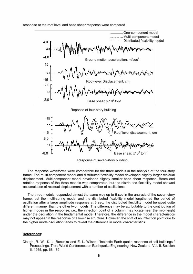
5

response at the roof level and base shear response were compared.

The response waveforms were comparable for the three models in the analysis of the four-story

frame. The multi-component model and distributed flexibility model developed slightly larger residual displacement. Multi-component model developed slightly smaller base shear response. Beam end rotation response of the three models was comparable, but the distributed flexibility model showed accumulation of residual displacement with a number of oscillations.

The three models responded almost the same way up to 6 sec in the analysis of the seven-story frame, but the multi-spring model and the distributed flexibility model lengthened the period of oscillation after a large amplitude response at 6 sec; the distributed flexibility model behaved quite different manner than the other two models. The difference may be attributable to the contribution of higher modes in the response; i.e., the inflection point of a column may locate near the mid-height under the oscillation in the fundamental mode. Therefore, the difference in the model characteristics may not appear in the response of a low-rise structure. However, the shift of an inflection point due to the higher mode oscillation tends to reveal the difference in model characteristics. References:

Clough, R. W., K. L. Benuska and E. L. Wilson, "Inelastic Earth-quake response of tall buildings,"

Proceedings, Third World Conference on Earthquake Engineering, New Zealand, Vol. II, Session II, 1965, pp. 68 - 89.

Roof level displacement, cm

Base shear, x103 tonf

Response of seven-story building

15

-15

8.0

-8.0

Ground motion acceleration, m/sec2

Roof-level Displacement, cm

Reponse of four-story building

Base shear, x 103 tonf

4.0

-4.0

15

-15 2.0

-2.0

One-component model Multi-component model Distributed flexibility model

6

Clough, R. W., and S. B. Johnston, "Effect of Stiffness Degradation on Earthquake Ductility Requirements," Proceedings, Second Japan Conference of Earthquake Engineering, October 1966, pp. 227 - 232.

Giberson, M. F., "The Response of Nonlinear Multi-story Structures subjected to Earthquake Excitation," EERL Report, Earthquake Engineering Research Laboratory, California Institute of Technology, Pasadena, 1967.

Kabeyasawa, T., "U.S.-Japan Cooperative Research, - Study on the Earthquake Resistance of Seven-story Reinforced Concrete Structure (Part 3: Pseudo-Dynamic Analysis) (in Japanese)," Proceedings, Sixth Japan Conference of Earthquake Engineering, December 1982, pp. 1161 - 1168.

Shiohara, H., S. Otani and H. Aoyama, "Comparison of Various Member Models for Reinforced Concrete Earthquake Response Analysis," Transactions, Japan Concrete Institute, Vol. 5, 1983, pp. 269 - 276.

Shiohara, H., S. Otani and H. Aoyama, "Comparison of Various Member Models for Reinforced Concrete Earthquake Response Analysis," Transactions, Japan Concrete Institute, Vol. 5, 1983, pp. 269 - 276.

Takeda, T., M. A. Sozen and N. N. Nielsen, "Reinforced Concrete Response to Simulated Earthquakes," Journal, Structural Division, ASCE, Vol. 96, No. ST12. December 1970, pp. 2557 - 2573.

Takizawa, H., "Notes on Some Basic Problems in Inelastic Analysis of Planar R/C Structures (Part 1)," Transactions, Architectural Institute of Japan, No. 240, February 1976, pp. 51 - 62.

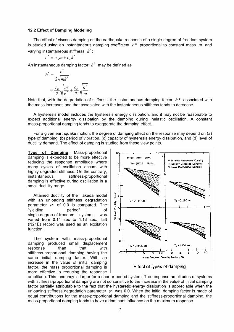
7

12.2 Effect of Damping Modeling

The effect of viscous damping on the earthquake response of a single-degree-of-freedom system is studied using an instantaneous damping coefficient *c proportional to constant mass m and varying instantaneous stiffness *k : ** kcmcc km +=

An instantaneous damping factor *h may be defined as

mkc

kmc

mkch

km*

*

*

**

22

2

+=

=

Note that, with the degradation of stiffness, the instantaneous damping factor *h associated with the mass increases and that associated with the instantaneous stiffness tends to decrease.

A hysteresis model includes the hysteresis energy dissipation, and it may not be reasonable to expect additional energy dissipation by the damping during inelastic oscillation. A constant mass-proportional damping tends to exaggerate the damping effect.

For a given earthquake motion, the degree of damping effect on the response may depend on (a) type of damping, (b) period of vibration, (c) capacity of hysteresis energy dissipation, and (d) level of ductility demand. The effect of damping is studied from these view points. Type of Damping: Mass-proportional damping is expected to be more effective reducing the response amplitude where many cycles of oscillation occurs with highly degraded stiffness. On the contrary, instantaneous stiffness-proportional damping is effective during oscillation in a small ductility range.

Attained ductility of the Takeda model with an unloading stiffness degradation parameter α of 0.0 is compared. The "yielding period" of single-degree-of-freedom systems was varied from 0.14 sec to 1.13 sec. Taft (N21E) record was used as an excitation function.

The system with mass-proportional damping produced small displacement response than that with stiffness-proportional damping having the same initial damping factor. With an increase in the value of initial damping factor, the mass proportional damping is more effective in reducing the response amplitude. This tendency is larger for a shorter period system. The response amplitudes of systems with stiffness-proportional damping are not so sensitive to the increase in the value of initial damping factor partially attributable to the fact that the hysteretic energy dissipation is appreciable when the unloading stiffness degradation parameter α was 0.0. When the initial damping factor is made of equal contributions for the mass-proportional damping and the stiffness-proportional damping, the mass-proportional damping tends to have a dominant influence on the maximum response.

Effect of types of damping

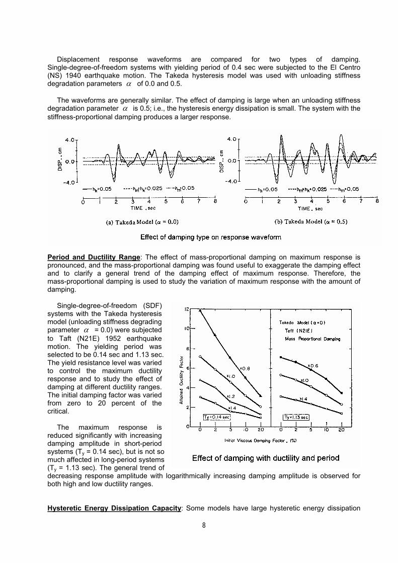
8

Displacement response waveforms are compared for two types of damping.

Single-degree-of-freedom systems with yielding period of 0.4 sec were subjected to the El Centro (NS) 1940 earthquake motion. The Takeda hysteresis model was used with unloading stiffness degradation parameters α of 0.0 and 0.5.

The waveforms are generally similar. The effect of damping is large when an unloading stiffness degradation parameter α is 0.5; i.e., the hysteresis energy dissipation is small. The system with the stiffness-proportional damping produces a larger response.

Period and Ductility Range: The effect of mass-proportional damping on maximum response is pronounced, and the mass-proportional damping was found useful to exaggerate the damping effect and to clarify a general trend of the damping effect of maximum response. Therefore, the mass-proportional damping is used to study the variation of maximum response with the amount of damping.

Single-degree-of-freedom (SDF) systems with the Takeda hysteresis model (unloading stiffness degrading parameter α = 0.0) were subjected to Taft (N21E) 1952 earthquake motion. The yielding period was selected to be 0.14 sec and 1.13 sec. The yield resistance level was varied to control the maximum ductility response and to study the effect of damping at different ductility ranges. The initial damping factor was varied from zero to 20 percent of the critical.

The maximum response is

reduced significantly with increasing damping amplitude in short-period systems (Ty = 0.14 sec), but is not so much affected in long-period systems (Ty = 1.13 sec). The general trend of decreasing response amplitude with logarithmically increasing damping amplitude is observed for both high and low ductility ranges. Hysteretic Energy Dissipation Capacity: Some models have large hysteretic energy dissipation

Effect of damping with yield level and period

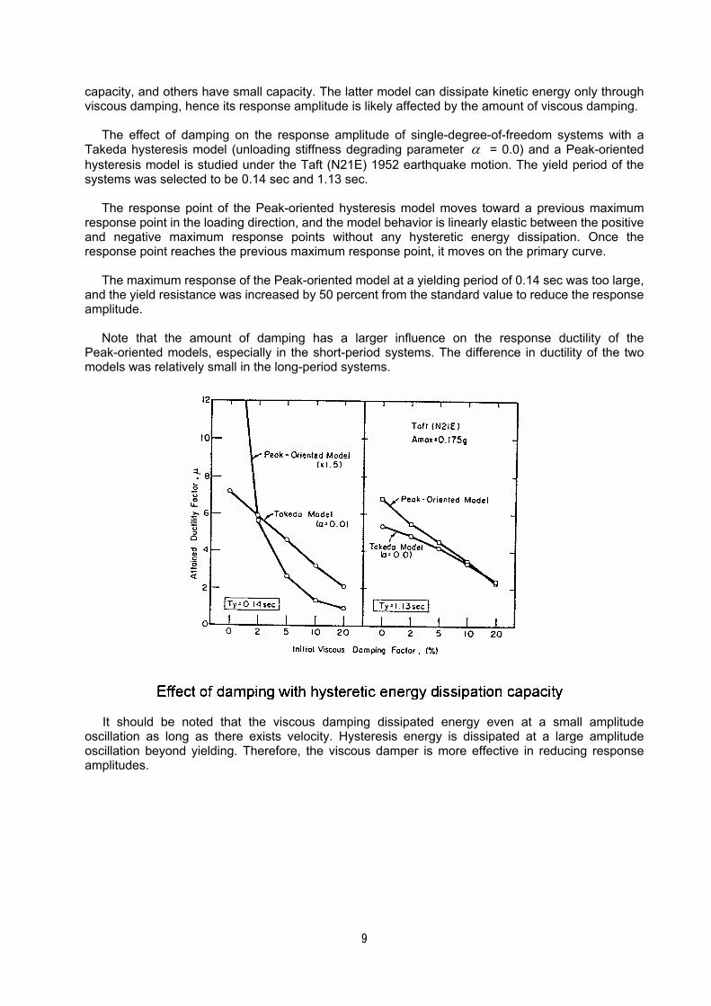
9

capacity, and others have small capacity. The latter model can dissipate kinetic energy only through viscous damping, hence its response amplitude is likely affected by the amount of viscous damping.

The effect of damping on the response amplitude of single-degree-of-freedom systems with a Takeda hysteresis model (unloading stiffness degrading parameter α = 0.0) and a Peak-oriented hysteresis model is studied under the Taft (N21E) 1952 earthquake motion. The yield period of the systems was selected to be 0.14 sec and 1.13 sec.

The response point of the Peak-oriented hysteresis model moves toward a previous maximum response point in the loading direction, and the model behavior is linearly elastic between the positive and negative maximum response points without any hysteretic energy dissipation. Once the response point reaches the previous maximum response point, it moves on the primary curve.

The maximum response of the Peak-oriented model at a yielding period of 0.14 sec was too large, and the yield resistance was increased by 50 percent from the standard value to reduce the response amplitude.

Note that the amount of damping has a larger influence on the response ductility of the Peak-oriented models, especially in the short-period systems. The difference in ductility of the two models was relatively small in the long-period systems.

It should be noted that the viscous damping dissipated energy even at a small amplitude

oscillation as long as there exists velocity. Hysteresis energy is dissipated at a large amplitude oscillation beyond yielding. Therefore, the viscous damper is more effective in reducing response amplitudes.

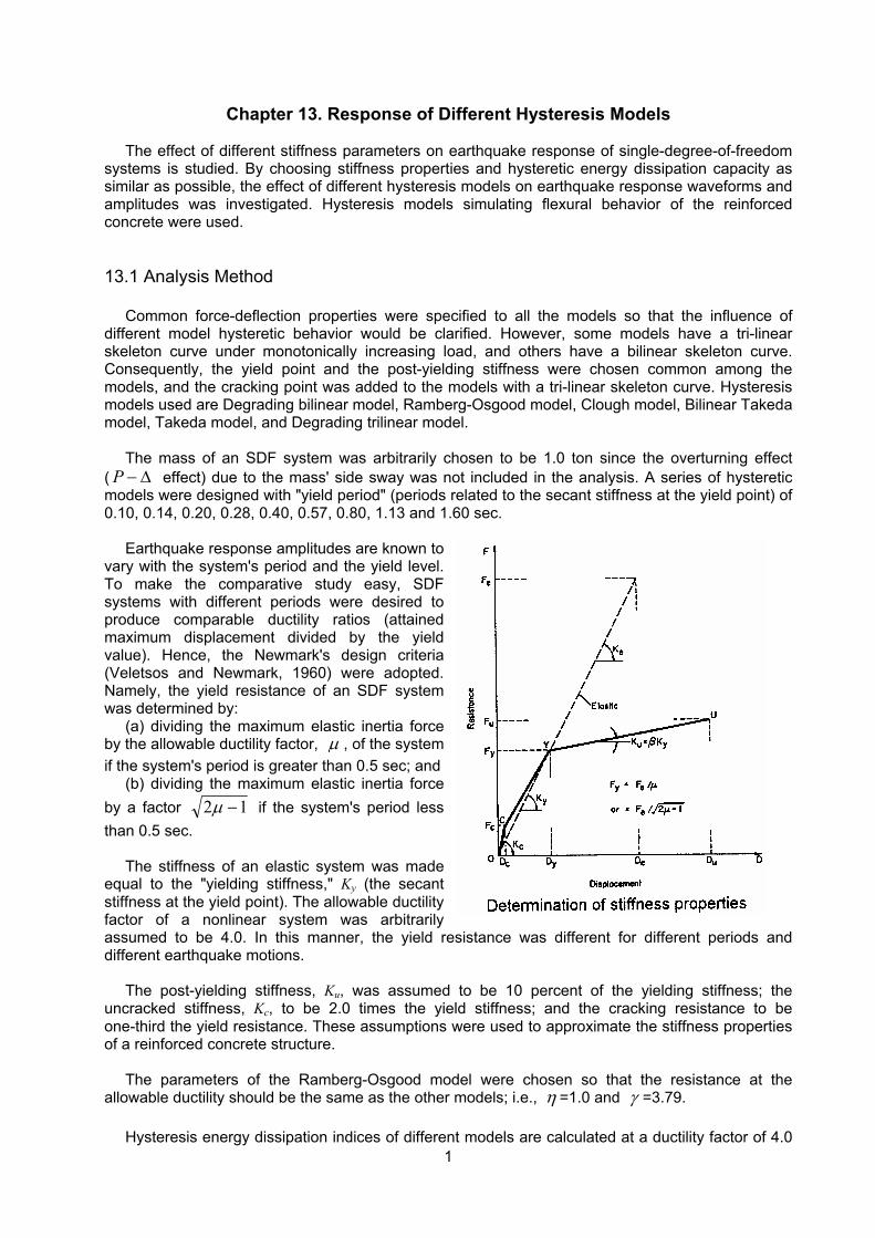
1

Chapter 13. Response of Different Hysteresis Models

The effect of different stiffness parameters on earthquake response of single-degree-of-freedom systems is studied. By choosing stiffness properties and hysteretic energy dissipation capacity as similar as possible, the effect of different hysteresis models on earthquake response waveforms and amplitudes was investigated. Hysteresis models simulating flexural behavior of the reinforced concrete were used. 13.1 Analysis Method

Common force-deflection properties were specified to all the models so that the influence of different model hysteretic behavior would be clarified. However, some models have a tri-linear skeleton curve under monotonically increasing load, and others have a bilinear skeleton curve. Consequently, the yield point and the post-yielding stiffness were chosen common among the models, and the cracking point was added to the models with a tri-linear skeleton curve. Hysteresis models used are Degrading bilinear model, Ramberg-Osgood model, Clough model, Bilinear Takeda model, Takeda model, and Degrading trilinear model.

The mass of an SDF system was arbitrarily chosen to be 1.0 ton since the overturning effect ( ∆−P effect) due to the mass' side sway was not included in the analysis. A series of hysteretic models were designed with "yield period" (periods related to the secant stiffness at the yield point) of 0.10, 0.14, 0.20, 0.28, 0.40, 0.57, 0.80, 1.13 and 1.60 sec.

Earthquake response amplitudes are known to vary with the system's period and the yield level. To make the comparative study easy, SDF systems with different periods were desired to produce comparable ductility ratios (attained maximum displacement divided by the yield value). Hence, the Newmark's design criteria (Veletsos and Newmark, 1960) were adopted. Namely, the yield resistance of an SDF system was determined by:

(a) dividing the maximum elastic inertia force by the allowable ductility factor, µ , of the system if the system's period is greater than 0.5 sec; and

(b) dividing the maximum elastic inertia force by a factor 12 −µ if the system's period less than 0.5 sec.

The stiffness of an elastic system was made equal to the "yielding stiffness," Ky (the secant stiffness at the yield point). The allowable ductility factor of a nonlinear system was arbitrarily assumed to be 4.0. In this manner, the yield resistance was different for different periods and different earthquake motions.

The post-yielding stiffness, Ku, was assumed to be 10 percent of the yielding stiffness; the uncracked stiffness, Kc, to be 2.0 times the yield stiffness; and the cracking resistance to be one-third the yield resistance. These assumptions were used to approximate the stiffness properties of a reinforced concrete structure.

The parameters of the Ramberg-Osgood model were chosen so that the resistance at the allowable ductility should be the same as the other models; i.e., η =1.0 and γ =3.79.

Hysteresis energy dissipation indices of different models are calculated at a ductility factor of 4.0

Determination of stiffness properties

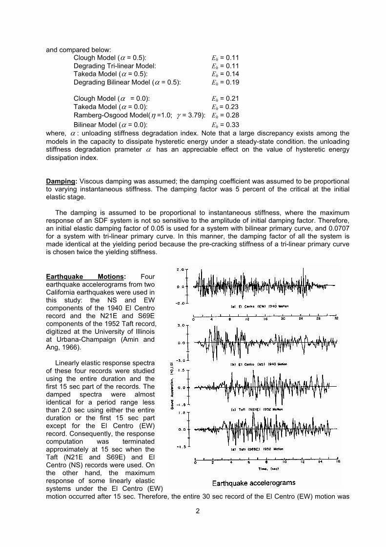
2

and compared below: Clough Model (α = 0.5): Eh = 0.11 Degrading Tri-linear Model: Eh = 0.11 Takeda Model (α = 0.5): Eh = 0.14 Degrading Bilinear Model (α = 0.5): Eh = 0.19 Clough Model (α = 0.0): Eh = 0.21 Takeda Model (α = 0.0): Eh = 0.23 Ramberg-Osgood Model(η =1.0; γ = 3.79): Eh = 0.28 Bilinear Model (α = 0.0): Eh = 0.33 where, α : unloading stiffness degradation index. Note that a large discrepancy exists among the models in the capacity to dissipate hysteretic energy under a steady-state condition. the unloading stiffness degradation prameter α has an appreciable effect on the value of hysteretic energy dissipation index. Damping: Viscous damping was assumed; the damping coefficient was assumed to be proportional to varying instantaneous stiffness. The damping factor was 5 percent of the critical at the initial elastic stage.

The damping is assumed to be proportional to instantaneous stiffness, where the maximum response of an SDF system is not so sensitive to the amplitude of initial damping factor. Therefore, an initial elastic damping factor of 0.05 is used for a system with bilinear primary curve, and 0.0707 for a system with tri-linear primary curve. In this manner, the damping factor of all the system is made identical at the yielding period because the pre-cracking stiffness of a tri-linear primary curve is chosen twice the yielding stiffness. Earthquake Motions: Four earthquake accelerograms from two California earthquakes were used in this study: the NS and EW components of the 1940 El Centro record and the N21E and S69E components of the 1952 Taft record, digitized at the University of Illinois at Urbana-Champaign (Amin and Ang, 1966).

Linearly elastic response spectra of these four records were studied using the entire duration and the first 15 sec part of the records. The damped spectra were almost identical for a period range less than 2.0 sec using either the entire duration or the first 15 sec part except for the El Centro (EW) record. Consequently, the response computation was terminated approximately at 15 sec when the Taft (N21E and S69E) and El Centro (NS) records were used. On the other hand, the maximum response of some linearly elastic systems under the El Centro (EW) motion occurred after 15 sec. Therefore, the entire 30 sec record of the El Centro (EW) motion was

Earthquake accelerograms

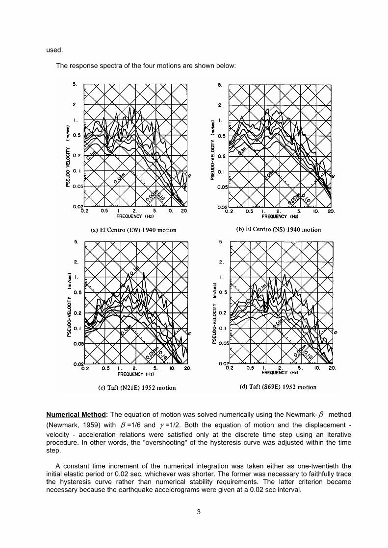
3

used.

The response spectra of the four motions are shown below:

Numerical Method: The equation of motion was solved numerically using the Newmark- β method (Newmark, 1959) with β =1/6 and γ =1/2. Both the equation of motion and the displacement - velocity - acceleration relations were satisfied only at the discrete time step using an iterative procedure. In other words, the "overshooting" of the hysteresis curve was adjusted within the time step.

A constant time increment of the numerical integration was taken either as one-twentieth the initial elastic period or 0.02 sec, whichever was shorter. The former was necessary to faithfully trace the hysteresis curve rather than numerical stability requirements. The latter criterion became necessary because the earthquake accelerograms were given at a 0.02 sec interval.

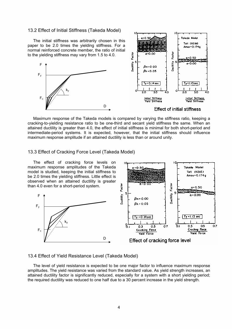
4

13.2 Effect of Initial Stiffness (Takeda Model)

The initial stiffness was arbitrarily chosen in this paper to be 2.0 times the yielding stiffness. For a normal reinforced concrete member, the ratio of initial to the yielding stiffness may vary from 1.5 to 4.0.

Fy

Fc

ky

D

F

Maximum response of the Takeda models is compared by varying the stiffness ratio, keeping a

cracking-to-yielding resistance ratio to be one-third and secant yield stiffness the same. When an attained ductility is greater than 4.0, the effect of initial stiffness is minimal for both short-period and intermediate-period systems. It is expected, however, that the initial stiffness should influence maximum response amplitude if an attained ductility is less than or around unity. 13.3 Effect of Cracking Force Level (Takeda Model)

The effect of cracking force levels on maximum response amplitudes of the Takeda model is studied, keeping the initial stiffness to be 2.0 times the yielding stiffness. Little effect is observed when an attained ductility is greater than 4.0 even for a short-period system.

Fy

Fc

ky

D

F

13.4 Effect of Yield Resistance Level (Takeda Model)

The level of yield resistance is expected to be one major factor to influence maximum response amplitudes. The yield resistance was varied from the standard value. As yield strength increases, an attained ductility factor is significantly reduced, especially for a system with a short yielding period; the required ductility was reduced to one half due to a 30 percent increase in the yield strength.

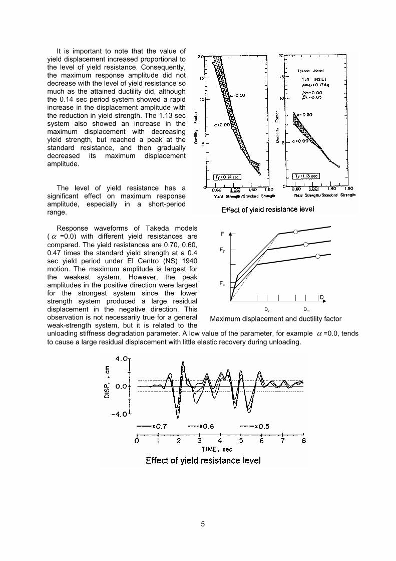
5

It is important to note that the value of yield displacement increased proportional to the level of yield resistance. Consequently, the maximum response amplitude did not decrease with the level of yield resistance so much as the attained ductility did, although the 0.14 sec period system showed a rapid increase in the displacement amplitude with the reduction in yield strength. The 1.13 sec system also showed an increase in the maximum displacement with decreasing yield strength, but reached a peak at the standard resistance, and then gradually decreased its maximum displacement amplitude.

The level of yield resistance has a significant effect on maximum response amplitude, especially in a short-period range.

Response waveforms of Takeda models ( α =0.0) with different yield resistances are compared. The yield resistances are 0.70, 0.60, 0.47 times the standard yield strength at a 0.4 sec yield period under El Centro (NS) 1940 motion. The maximum amplitude is largest for the weakest system. However, the peak amplitudes in the positive direction were largest for the strongest system since the lower strength system produced a large residual displacement in the negative direction. This observation is not necessarily true for a general weak-strength system, but it is related to the unloading stiffness degradation parameter. A low value of the parameter, for example α =0.0, tends to cause a large residual displacement with little elastic recovery during unloading.

Fy

Fc

D

F

Dy Dm Maximum displacement and ductility factor

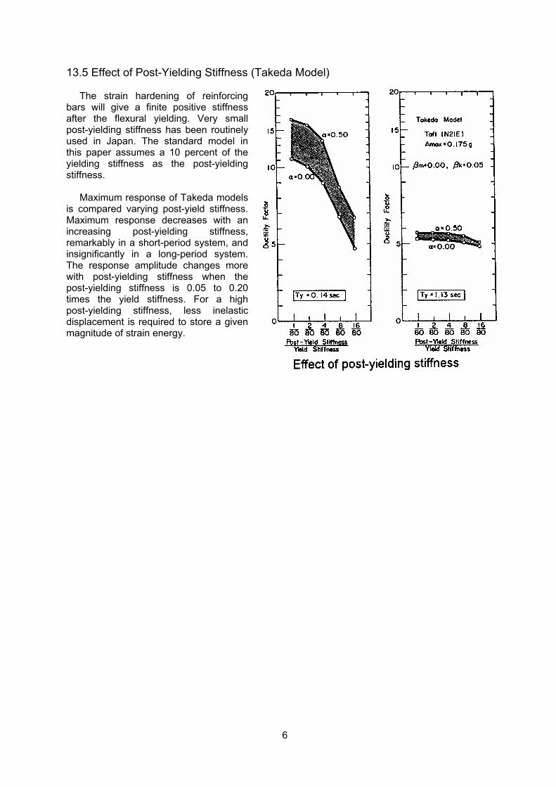
6

13.5 Effect of Post-Yielding Stiffness (Takeda Model) The strain hardening of reinforcing

bars will give a finite positive stiffness after the flexural yielding. Very small post-yielding stiffness has been routinely used in Japan. The standard model in this paper assumes a 10 percent of the yielding stiffness as the post-yielding stiffness.

Maximum response of Takeda models is compared varying post-yield stiffness. Maximum response decreases with an increasing post-yielding stiffness, remarkably in a short-period system, and insignificantly in a long-period system. The response amplitude changes more with post-yielding stiffness when the post-yielding stiffness is 0.05 to 0.20 times the yield stiffness. For a high post-yielding stiffness, less inelastic displacement is required to store a given magnitude of strain energy.

Effect of post-yielding stiffness

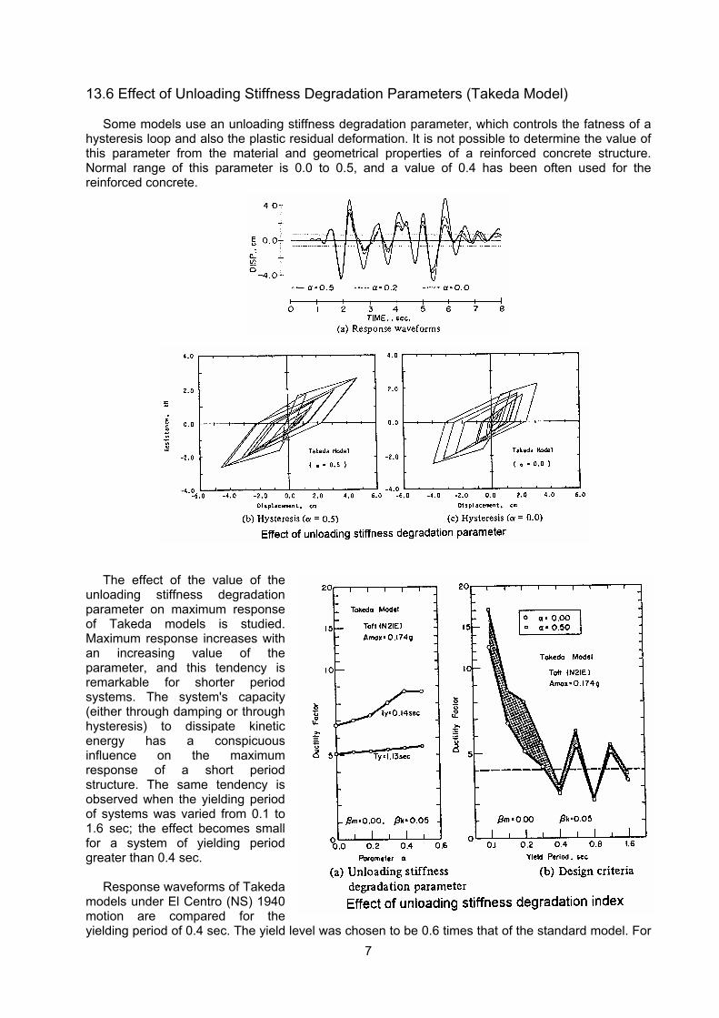
7

13.6 Effect of Unloading Stiffness Degradation Parameters (Takeda Model)

Some models use an unloading stiffness degradation parameter, which controls the fatness of a hysteresis loop and also the plastic residual deformation. It is not possible to determine the value of this parameter from the material and geometrical properties of a reinforced concrete structure. Normal range of this parameter is 0.0 to 0.5, and a value of 0.4 has been often used for the reinforced concrete.

The effect of the value of the

unloading stiffness degradation parameter on maximum response of Takeda models is studied. Maximum response increases with an increasing value of the parameter, and this tendency is remarkable for shorter period systems. The system's capacity (either through damping or through hysteresis) to dissipate kinetic energy has a conspicuous influence on the maximum response of a short period structure. The same tendency is observed when the yielding period of systems was varied from 0.1 to 1.6 sec; the effect becomes small for a system of yielding period greater than 0.4 sec.

Response waveforms of Takeda models under El Centro (NS) 1940 motion are compared for the yielding period of 0.4 sec. The yield level was chosen to be 0.6 times that of the standard model. For

8

a large value of the parameter, peak amplitudes are larger both in the positive and negative directions, having comparable amplitudes in the two directions. For smaller values of the parameter, the system tends to produce large amplitude only in one direction. This is clearly observed in the hysteretic curve. Peak-to-peak stiffness in a low amplitude oscillation is lower for a system with a larger parameter, causing a long period of oscillation from approximately 6.0 sec.

The effect of the unloading stiffness degradation parameter is significant on response amplitude, response waveform, residual displacement and hysteresis shape.

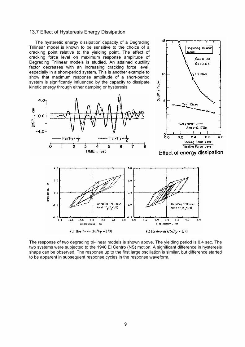
9

13.7 Effect of Hysteresis Energy Dissipation

The hysteretic energy dissipation capacity of a Degrading Trilinear model is known to be sensitive to the choice of a cracking point relative to the yielding point. The effect of cracking force level on maximum response amplitude of Degrading Trilinear models is studied. An attained ductility factor decreases with an increasing cracking force level, especially in a short-period system. This is another example to show that maximum response amplitude of a short-period system is significantly influenced by the capacity to dissipate kinetic energy through either damping or hysteresis.

The response of two degrading tri-linear models is shown above. The yielding period is 0.4 sec. The two systems were subjected to the 1940 El Centro (NS) motion. A significant difference in hysteresis shape can be observed. The response up to the first large oscillation is similar, but difference started to be apparent in subsequent response cycles in the response waveform.

Effect of energy dissipation

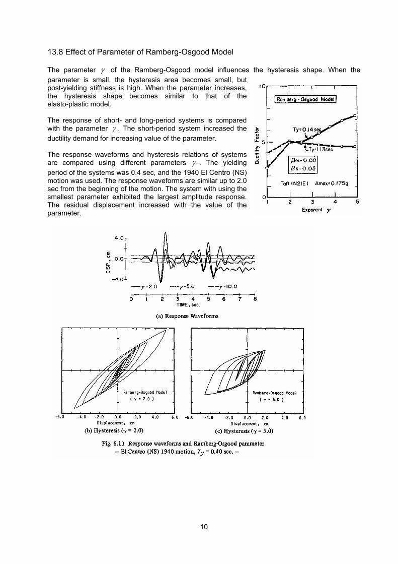
10

13.8 Effect of Parameter of Ramberg-Osgood Model The parameter γ of the Ramberg-Osgood model influences the hysteresis shape. When the parameter is small, the hysteresis area becomes small, but post-yielding stiffness is high. When the parameter increases, the hysteresis shape becomes similar to that of the elasto-plastic model. The response of short- and long-period systems is compared with the parameter γ . The short-period system increased the ductility demand for increasing value of the parameter. The response waveforms and hysteresis relations of systems are compared using different parameters γ . The yielding period of the systems was 0.4 sec, and the 1940 El Centro (NS) motion was used. The response waveforms are similar up to 2.0 sec from the beginning of the motion. The system with using the smallest parameter exhibited the largest amplitude response. The residual displacement increased with the value of the parameter.

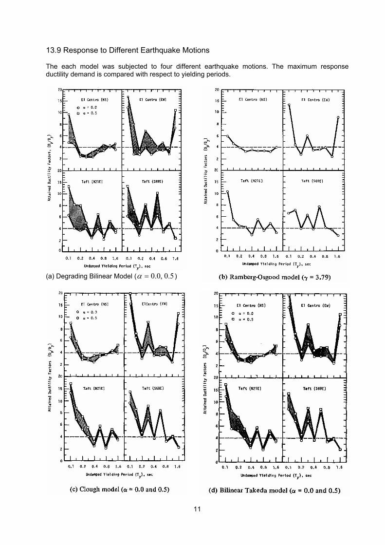
11

13.9 Response to Different Earthquake Motions The each model was subjected to four different earthquake motions. The maximum response ductility demand is compared with respect to yielding periods.

(a) Degrading Bilinear Model ( 5.0,0.0=α )

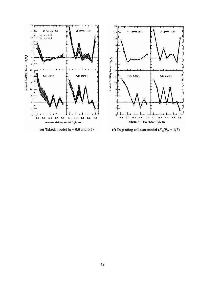
12

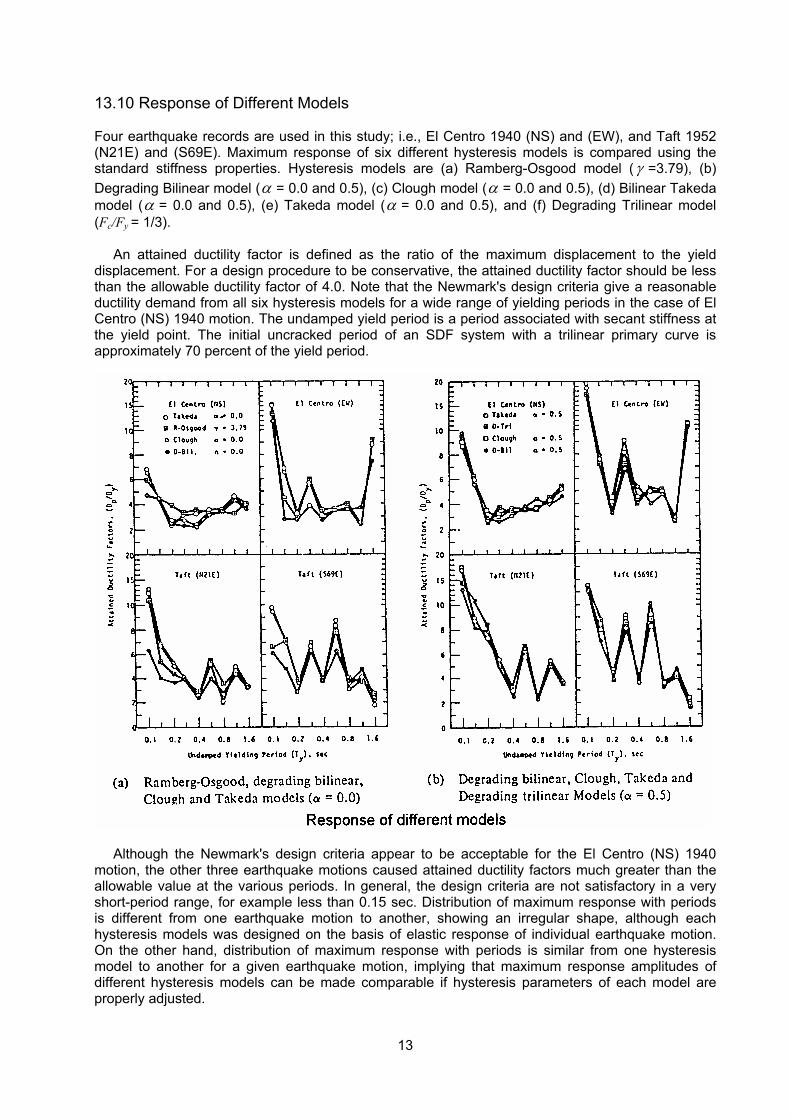
13

13.10 Response of Different Models Four earthquake records are used in this study; i.e., El Centro 1940 (NS) and (EW), and Taft 1952 (N21E) and (S69E). Maximum response of six different hysteresis models is compared using the standard stiffness properties. Hysteresis models are (a) Ramberg-Osgood model ( γ =3.79), (b) Degrading Bilinear model (α = 0.0 and 0.5), (c) Clough model (α = 0.0 and 0.5), (d) Bilinear Takeda model (α = 0.0 and 0.5), (e) Takeda model (α = 0.0 and 0.5), and (f) Degrading Trilinear model (Fc/Fy = 1/3).

An attained ductility factor is defined as the ratio of the maximum displacement to the yield displacement. For a design procedure to be conservative, the attained ductility factor should be less than the allowable ductility factor of 4.0. Note that the Newmark's design criteria give a reasonable ductility demand from all six hysteresis models for a wide range of yielding periods in the case of El Centro (NS) 1940 motion. The undamped yield period is a period associated with secant stiffness at the yield point. The initial uncracked period of an SDF system with a trilinear primary curve is approximately 70 percent of the yield period.

Although the Newmark's design criteria appear to be acceptable for the El Centro (NS) 1940

motion, the other three earthquake motions caused attained ductility factors much greater than the allowable value at the various periods. In general, the design criteria are not satisfactory in a very short-period range, for example less than 0.15 sec. Distribution of maximum response with periods is different from one earthquake motion to another, showing an irregular shape, although each hysteresis models was designed on the basis of elastic response of individual earthquake motion. On the other hand, distribution of maximum response with periods is similar from one hysteresis model to another for a given earthquake motion, implying that maximum response amplitudes of different hysteresis models can be made comparable if hysteresis parameters of each model are properly adjusted.

14

For an unloading stiffness degradation parameter of 0.5, the Takeda, Clough and Degrading Bilinear models developed comparable ductility factors. The Degrading Trilinear model also developed ductility factors similar in magnitude to those three models at corresponding periods.

Therefore, maximum response amplitudes are not as sensitive to detail difference in hysteretic rules of these models, but rather are influenced by more basic characteristics of hysteresis loops, such as stiffness properties to define a primary curve and the fatness (hysteretic energy dissipating capacity) of a hysteresis loop.

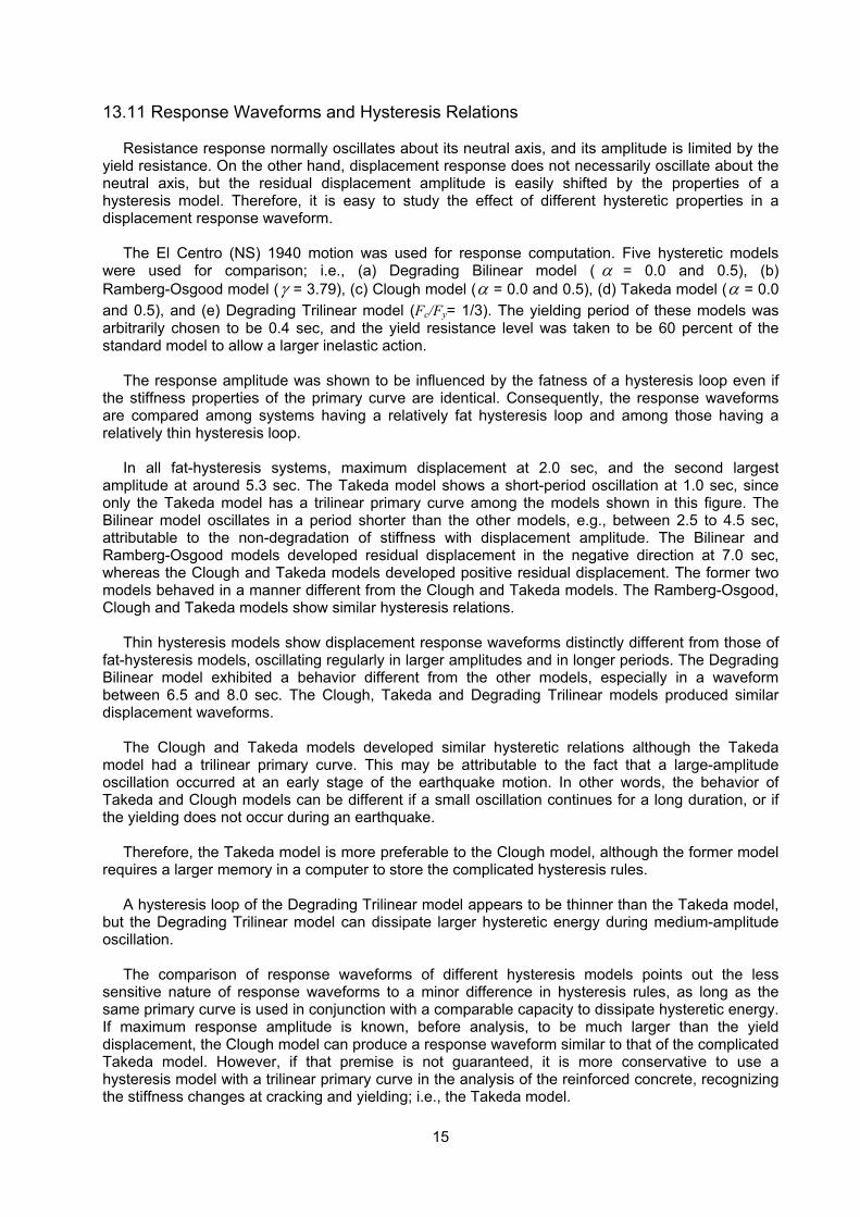
15

13.11 Response Waveforms and Hysteresis Relations Resistance response normally oscillates about its neutral axis, and its amplitude is limited by the

yield resistance. On the other hand, displacement response does not necessarily oscillate about the neutral axis, but the residual displacement amplitude is easily shifted by the properties of a hysteresis model. Therefore, it is easy to study the effect of different hysteretic properties in a displacement response waveform.

The El Centro (NS) 1940 motion was used for response computation. Five hysteretic models were used for comparison; i.e., (a) Degrading Bilinear model ( α = 0.0 and 0.5), (b) Ramberg-Osgood model (γ = 3.79), (c) Clough model (α = 0.0 and 0.5), (d) Takeda model (α = 0.0 and 0.5), and (e) Degrading Trilinear model (Fc/Fy= 1/3). The yielding period of these models was arbitrarily chosen to be 0.4 sec, and the yield resistance level was taken to be 60 percent of the standard model to allow a larger inelastic action.

The response amplitude was shown to be influenced by the fatness of a hysteresis loop even if the stiffness properties of the primary curve are identical. Consequently, the response waveforms are compared among systems having a relatively fat hysteresis loop and among those having a relatively thin hysteresis loop.

In all fat-hysteresis systems, maximum displacement at 2.0 sec, and the second largest amplitude at around 5.3 sec. The Takeda model shows a short-period oscillation at 1.0 sec, since only the Takeda model has a trilinear primary curve among the models shown in this figure. The Bilinear model oscillates in a period shorter than the other models, e.g., between 2.5 to 4.5 sec, attributable to the non-degradation of stiffness with displacement amplitude. The Bilinear and Ramberg-Osgood models developed residual displacement in the negative direction at 7.0 sec, whereas the Clough and Takeda models developed positive residual displacement. The former two models behaved in a manner different from the Clough and Takeda models. The Ramberg-Osgood, Clough and Takeda models show similar hysteresis relations.

Thin hysteresis models show displacement response waveforms distinctly different from those of fat-hysteresis models, oscillating regularly in larger amplitudes and in longer periods. The Degrading Bilinear model exhibited a behavior different from the other models, especially in a waveform between 6.5 and 8.0 sec. The Clough, Takeda and Degrading Trilinear models produced similar displacement waveforms.

The Clough and Takeda models developed similar hysteretic relations although the Takeda model had a trilinear primary curve. This may be attributable to the fact that a large-amplitude oscillation occurred at an early stage of the earthquake motion. In other words, the behavior of Takeda and Clough models can be different if a small oscillation continues for a long duration, or if the yielding does not occur during an earthquake.

Therefore, the Takeda model is more preferable to the Clough model, although the former model requires a larger memory in a computer to store the complicated hysteresis rules.

A hysteresis loop of the Degrading Trilinear model appears to be thinner than the Takeda model, but the Degrading Trilinear model can dissipate larger hysteretic energy during medium-amplitude oscillation.

The comparison of response waveforms of different hysteresis models points out the less sensitive nature of response waveforms to a minor difference in hysteresis rules, as long as the same primary curve is used in conjunction with a comparable capacity to dissipate hysteretic energy. If maximum response amplitude is known, before analysis, to be much larger than the yield displacement, the Clough model can produce a response waveform similar to that of the complicated Takeda model. However, if that premise is not guaranteed, it is more conservative to use a hysteresis model with a trilinear primary curve in the analysis of the reinforced concrete, recognizing the stiffness changes at cracking and yielding; i.e., the Takeda model.

16

References: Amin, M., and A. H.-S. Ang, "A Nonstationary Model for Strong Motion Earthquakes," Structural

Research Series No. 306, Civil Engineering Study, University of Illinois, Urbana, 1966. Otani, S, "Hysteresis Models of Reinforced Concrete for Earthquake Response Analysis," Journal,

Faculty of Engineering, University of Tokyo, Vol. XXXVI, No. 2, 1981, pp. 125-156. Newmark, N. M., "A Method of Computation for Structural Dynamics," Journal, Engineering

Mechanics Division, ASCE, Vol. 85, No. EM3, 1959, pp. 67-94. Veletsos, A. S., and N.M. Newmark, "Effect of Inelastic Behavior on the Response of Simple

Systems to Earthquake Motions," Proceedings, Second World Conference on Earthquake Engineering, 1960, Vol. II, pp. 895-912.

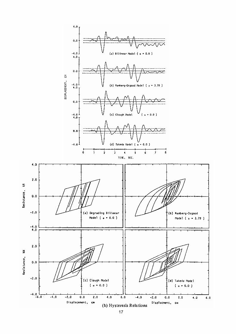
17

18

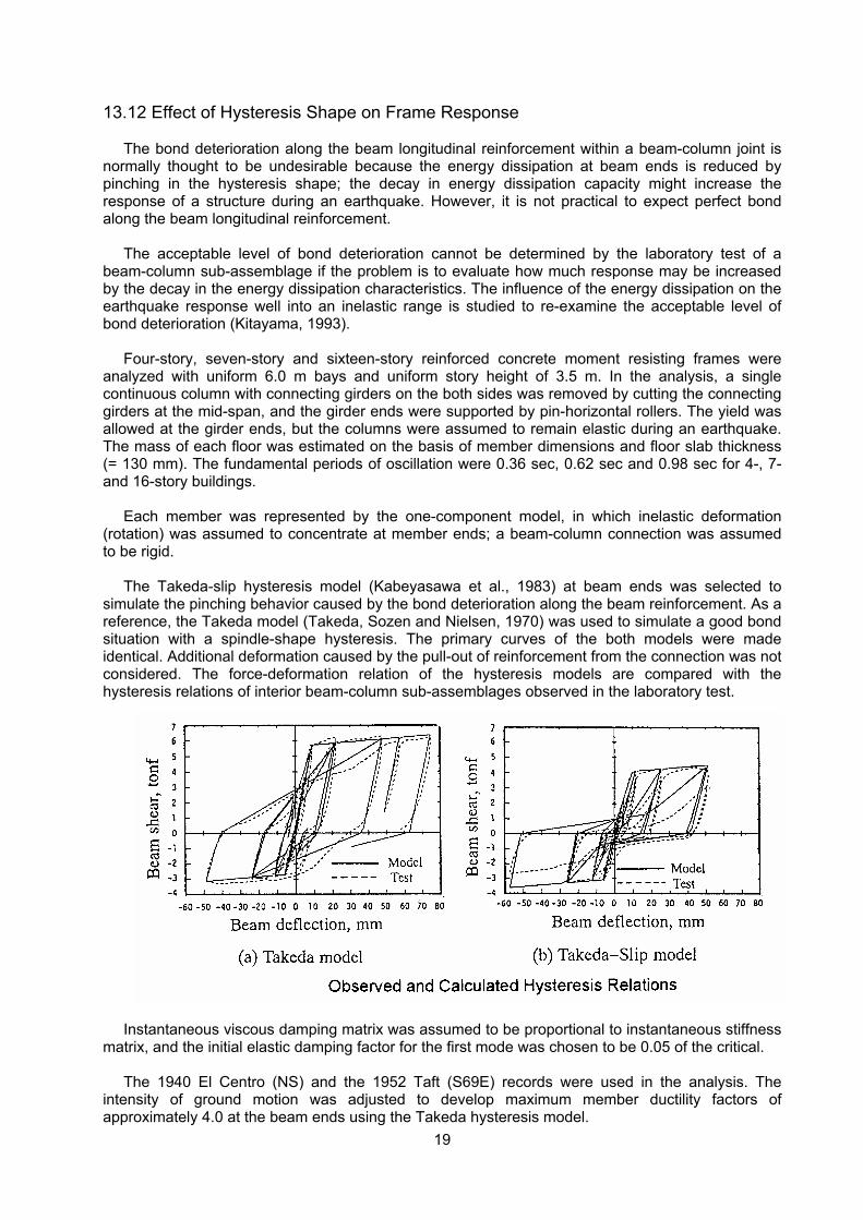
19

13.12 Effect of Hysteresis Shape on Frame Response

The bond deterioration along the beam longitudinal reinforcement within a beam-column joint is normally thought to be undesirable because the energy dissipation at beam ends is reduced by pinching in the hysteresis shape; the decay in energy dissipation capacity might increase the response of a structure during an earthquake. However, it is not practical to expect perfect bond along the beam longitudinal reinforcement.

The acceptable level of bond deterioration cannot be determined by the laboratory test of a beam-column sub-assemblage if the problem is to evaluate how much response may be increased by the decay in the energy dissipation characteristics. The influence of the energy dissipation on the earthquake response well into an inelastic range is studied to re-examine the acceptable level of bond deterioration (Kitayama, 1993).

Four-story, seven-story and sixteen-story reinforced concrete moment resisting frames were analyzed with uniform 6.0 m bays and uniform story height of 3.5 m. In the analysis, a single continuous column with connecting girders on the both sides was removed by cutting the connecting girders at the mid-span, and the girder ends were supported by pin-horizontal rollers. The yield was allowed at the girder ends, but the columns were assumed to remain elastic during an earthquake. The mass of each floor was estimated on the basis of member dimensions and floor slab thickness (= 130 mm). The fundamental periods of oscillation were 0.36 sec, 0.62 sec and 0.98 sec for 4-, 7- and 16-story buildings.

Each member was represented by the one-component model, in which inelastic deformation (rotation) was assumed to concentrate at member ends; a beam-column connection was assumed to be rigid.

The Takeda-slip hysteresis model (Kabeyasawa et al., 1983) at beam ends was selected to simulate the pinching behavior caused by the bond deterioration along the beam reinforcement. As a reference, the Takeda model (Takeda, Sozen and Nielsen, 1970) was used to simulate a good bond situation with a spindle-shape hysteresis. The primary curves of the both models were made identical. Additional deformation caused by the pull-out of reinforcement from the connection was not considered. The force-deformation relation of the hysteresis models are compared with the hysteresis relations of interior beam-column sub-assemblages observed in the laboratory test.

Instantaneous viscous damping matrix was assumed to be proportional to instantaneous stiffness

matrix, and the initial elastic damping factor for the first mode was chosen to be 0.05 of the critical.

The 1940 El Centro (NS) and the 1952 Taft (S69E) records were used in the analysis. The intensity of ground motion was adjusted to develop maximum member ductility factors of approximately 4.0 at the beam ends using the Takeda hysteresis model.

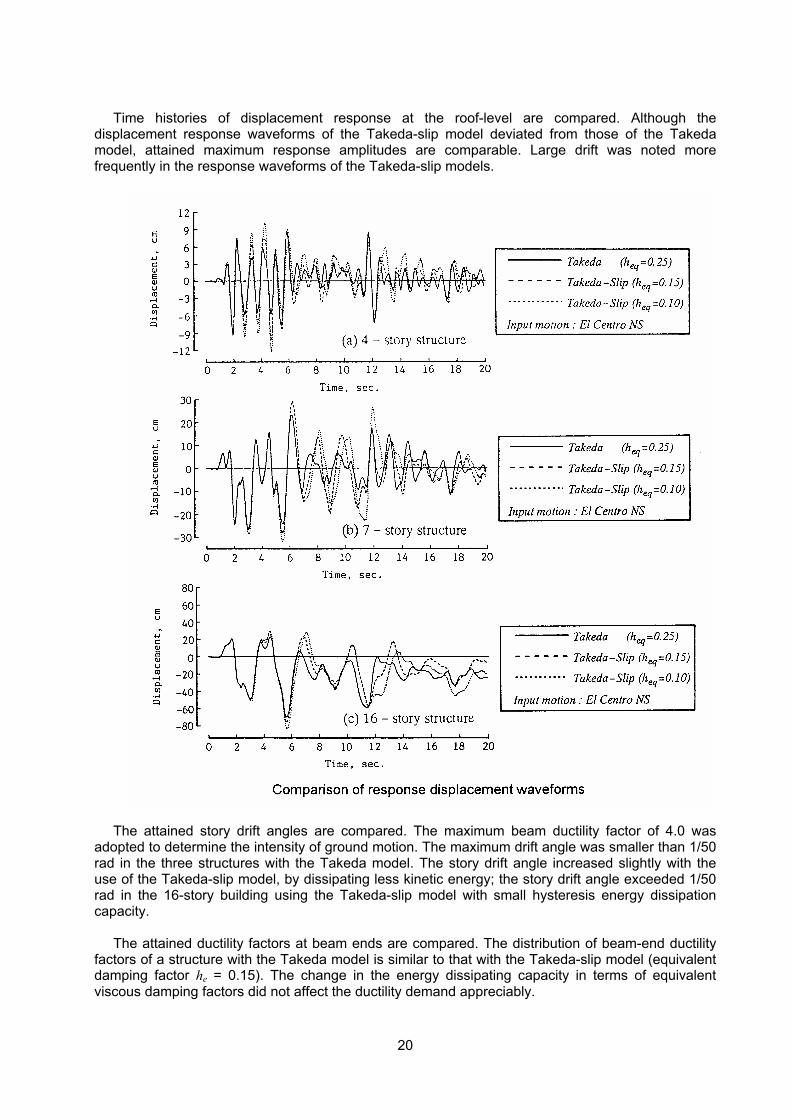
20

Time histories of displacement response at the roof-level are compared. Although the

displacement response waveforms of the Takeda-slip model deviated from those of the Takeda model, attained maximum response amplitudes are comparable. Large drift was noted more frequently in the response waveforms of the Takeda-slip models.

The attained story drift angles are compared. The maximum beam ductility factor of 4.0 was

adopted to determine the intensity of ground motion. The maximum drift angle was smaller than 1/50 rad in the three structures with the Takeda model. The story drift angle increased slightly with the use of the Takeda-slip model, by dissipating less kinetic energy; the story drift angle exceeded 1/50 rad in the 16-story building using the Takeda-slip model with small hysteresis energy dissipation capacity.

The attained ductility factors at beam ends are compared. The distribution of beam-end ductility factors of a structure with the Takeda model is similar to that with the Takeda-slip model (equivalent damping factor he = 0.15). The change in the energy dissipating capacity in terms of equivalent viscous damping factors did not affect the ductility demand appreciably.

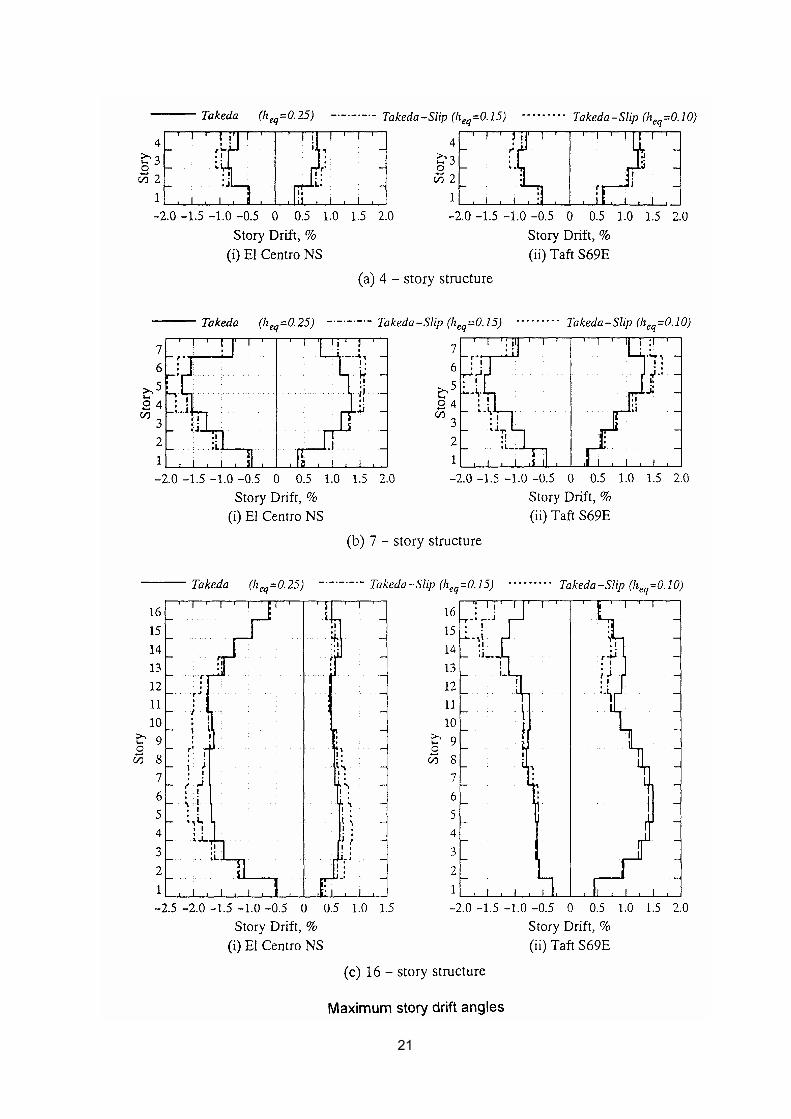
21

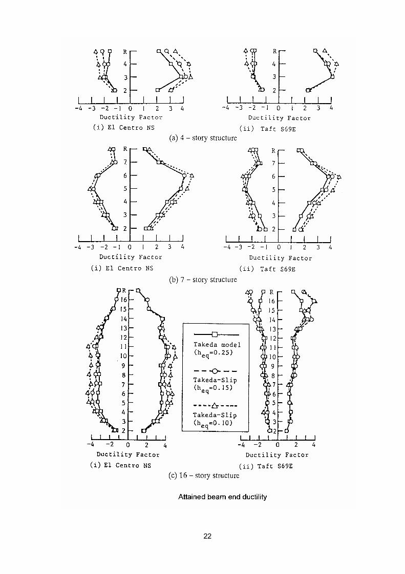
22

23

References: Giberson, M. F., "The Response of Nonlinear Multi-story Structures subjected to Earthquake

Excitation," EERL Report, Earthquake Engineering Research Laboratory, California Institute of Technology, Pasadena, 1967.

Kabeyasawa, T., H. Shiohara, S. Otani and H. Aoyama, "Analysis of the Full-scale Seven-story Reinforced Concrete Test Structure," Journal, Faculty of Engineering, University of Tokyo (B), Vol. XXXVII, No. 2, 1983, pp. 432-478.

Kitayama, K., "Limitation of Beam Bar Bond Deterioration within Beam-column Joint," Earthquake Resistance of Reinforced Concrete Structures, A Volume Honoring Hiroyuki Aoyama, November 1993, pp. 297 - 306.

Takeda, T., M. A. Sozen and N. N. Nielsen, "Reinforced Concrete Response to Simulated Earthquakes," Journal, Structural Division, ASCE, Vol. 96, No. ST12, 1970, pp. 2557-2573.

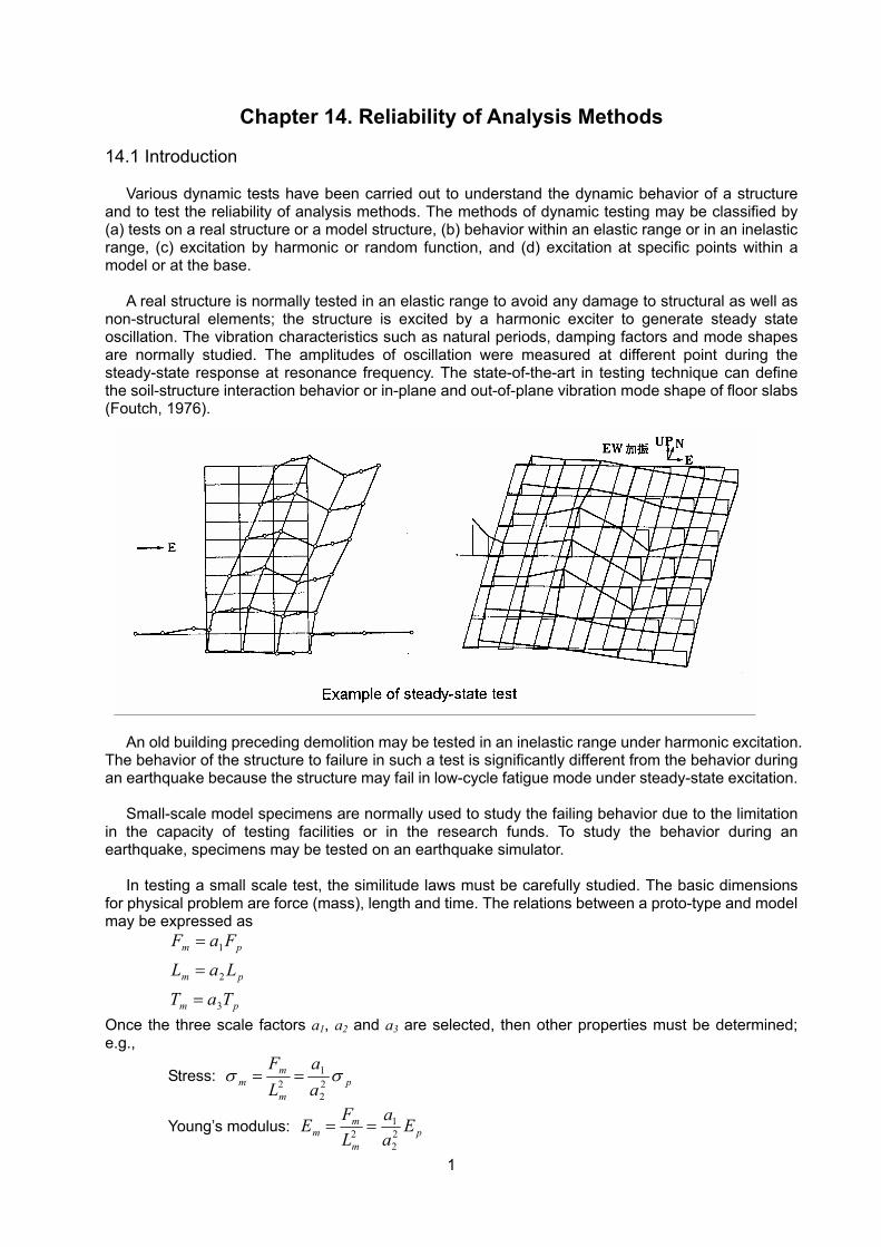
1

Chapter 14. Reliability of Analysis Methods 14.1 Introduction

Various dynamic tests have been carried out to understand the dynamic behavior of a structure and to test the reliability of analysis methods. The methods of dynamic testing may be classified by (a) tests on a real structure or a model structure, (b) behavior within an elastic range or in an inelastic range, (c) excitation by harmonic or random function, and (d) excitation at specific points within a model or at the base.

A real structure is normally tested in an elastic range to avoid any damage to structural as well as non-structural elements; the structure is excited by a harmonic exciter to generate steady state oscillation. The vibration characteristics such as natural periods, damping factors and mode shapes are normally studied. The amplitudes of oscillation were measured at different point during the steady-state response at resonance frequency. The state-of-the-art in testing technique can define the soil-structure interaction behavior or in-plane and out-of-plane vibration mode shape of floor slabs (Foutch, 1976).

An old building preceding demolition may be tested in an inelastic range under harmonic excitation.

The behavior of the structure to failure in such a test is significantly different from the behavior during an earthquake because the structure may fail in low-cycle fatigue mode under steady-state excitation.

Small-scale model specimens are normally used to study the failing behavior due to the limitation in the capacity of testing facilities or in the research funds. To study the behavior during an earthquake, specimens may be tested on an earthquake simulator.

In testing a small scale test, the similitude laws must be carefully studied. The basic dimensions for physical problem are force (mass), length and time. The relations between a proto-type and model may be expressed as

pm

pm

pm

TaT

LaL

FaF

3

2

1

=

=

=

Once the three scale factors a1, a2 and a3 are selected, then other properties must be determined; e.g.,

Stress: pm

mm a

aLF

σσ 22

12 ==

Young’s modulus: pm

mm E

aa

LFE 2

2

12 ==

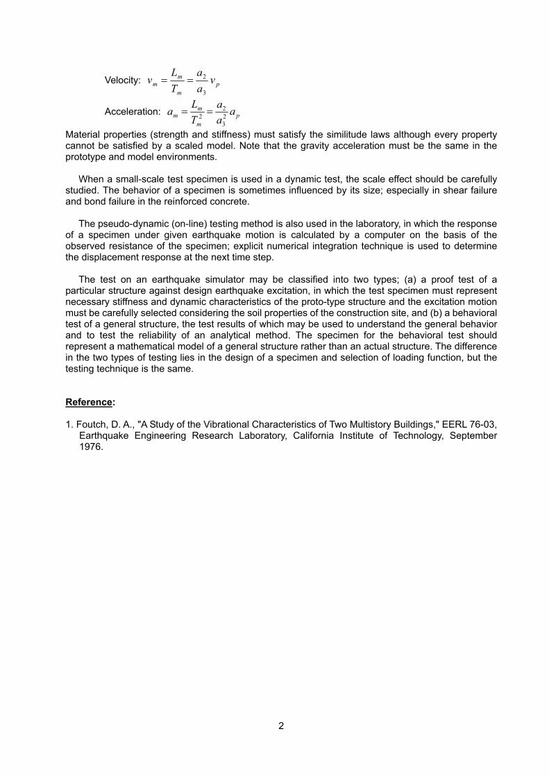
2

Velocity: pm

mm v

aa

TL

v3

2==

Acceleration: pm

mm a

aa

TLa 2

3

22 ==

Material properties (strength and stiffness) must satisfy the similitude laws although every property cannot be satisfied by a scaled model. Note that the gravity acceleration must be the same in the prototype and model environments.

When a small-scale test specimen is used in a dynamic test, the scale effect should be carefully studied. The behavior of a specimen is sometimes influenced by its size; especially in shear failure and bond failure in the reinforced concrete.

The pseudo-dynamic (on-line) testing method is also used in the laboratory, in which the response of a specimen under given earthquake motion is calculated by a computer on the basis of the observed resistance of the specimen; explicit numerical integration technique is used to determine the displacement response at the next time step.

The test on an earthquake simulator may be classified into two types; (a) a proof test of a particular structure against design earthquake excitation, in which the test specimen must represent necessary stiffness and dynamic characteristics of the proto-type structure and the excitation motion must be carefully selected considering the soil properties of the construction site, and (b) a behavioral test of a general structure, the test results of which may be used to understand the general behavior and to test the reliability of an analytical method. The specimen for the behavioral test should represent a mathematical model of a general structure rather than an actual structure. The difference in the two types of testing lies in the design of a specimen and selection of loading function, but the testing technique is the same. Reference: 1. Foutch, D. A., "A Study of the Vibrational Characteristics of Two Multistory Buildings," EERL 76-03,

Earthquake Engineering Research Laboratory, California Institute of Technology, September 1976.

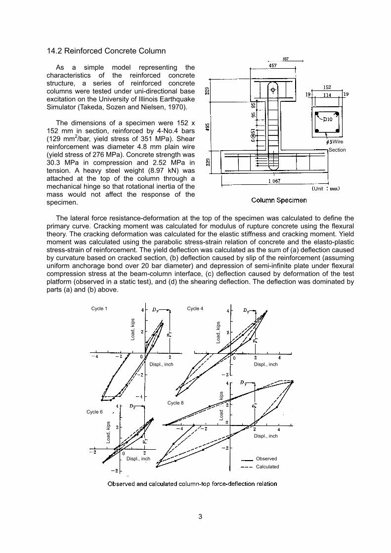
3

14.2 Reinforced Concrete Column

As a simple model representing the characteristics of the reinforced concrete structure, a series of reinforced concrete columns were tested under uni-directional base excitation on the University of Illinois Earthquake Simulator (Takeda, Sozen and Nielsen, 1970).

The dimensions of a specimen were 152 x 152 mm in section, reinforced by 4-No.4 bars (129 mm2/bar, yield stress of 351 MPa). Shear reinforcement was diameter 4.8 mm plain wire (yield stress of 276 MPa). Concrete strength was 30.3 MPa in compression and 2.52 MPa in tension. A heavy steel weight (8.97 kN) was attached at the top of the column through a mechanical hinge so that rotational inertia of the mass would not affect the response of the specimen.

The lateral force resistance-deformation at the top of the specimen was calculated to define the primary curve. Cracking moment was calculated for modulus of rupture concrete using the flexural theory. The cracking deformation was calculated for the elastic stiffness and cracking moment. Yield moment was calculated using the parabolic stress-strain relation of concrete and the elasto-plastic stress-strain of reinforcement. The yield deflection was calculated as the sum of (a) deflection caused by curvature based on cracked section, (b) deflection caused by slip of the reinforcement (assuming uniform anchorage bond over 20 bar diameter) and depression of semi-infinite plate under flexural compression stress at the beam-column interface, (c) deflection caused by deformation of the test platform (observed in a static test), and (d) the shearing deflection. The deflection was dominated by parts (a) and (b) above.

WireSection

Unit

Cycle 1 Cycle 4

Displ., inch Displ., inch

Displ., inch

Displ., inch

Observed Calculated

Load

, kip

s

Load

, kip

s

Load

, kip

s

Cycle 6

Cycle 8

Load

ki

ps

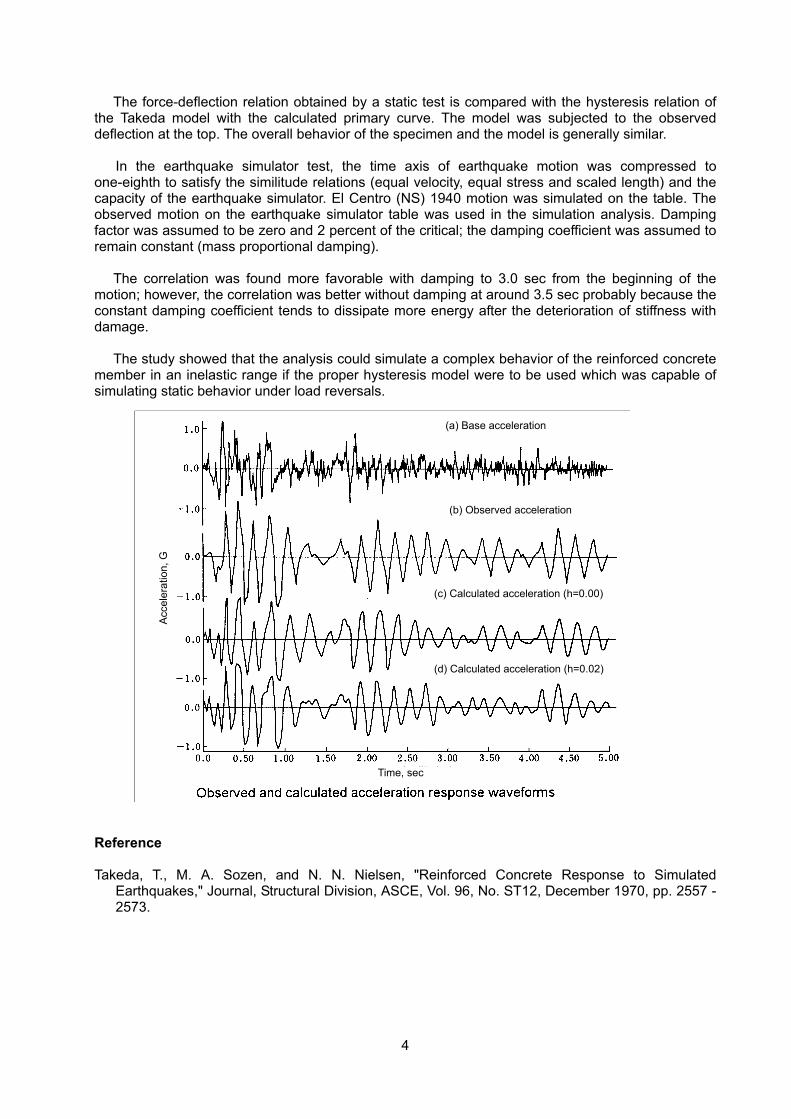
4

The force-deflection relation obtained by a static test is compared with the hysteresis relation of the Takeda model with the calculated primary curve. The model was subjected to the observed deflection at the top. The overall behavior of the specimen and the model is generally similar.

In the earthquake simulator test, the time axis of earthquake motion was compressed to one-eighth to satisfy the similitude relations (equal velocity, equal stress and scaled length) and the capacity of the earthquake simulator. El Centro (NS) 1940 motion was simulated on the table. The observed motion on the earthquake simulator table was used in the simulation analysis. Damping factor was assumed to be zero and 2 percent of the critical; the damping coefficient was assumed to remain constant (mass proportional damping).

The correlation was found more favorable with damping to 3.0 sec from the beginning of the motion; however, the correlation was better without damping at around 3.5 sec probably because the constant damping coefficient tends to dissipate more energy after the deterioration of stiffness with damage.

The study showed that the analysis could simulate a complex behavior of the reinforced concrete member in an inelastic range if the proper hysteresis model were to be used which was capable of simulating static behavior under load reversals.

Reference Takeda, T., M. A. Sozen, and N. N. Nielsen, "Reinforced Concrete Response to Simulated

Earthquakes," Journal, Structural Division, ASCE, Vol. 96, No. ST12, December 1970, pp. 2557 - 2573.

(a) Base acceleration

(b) Observed acceleration

(c) Calculated acceleration (h=0.00)

(d) Calculated acceleration (h=0.02)

Time, sec

Acc

eler

atio

n, G

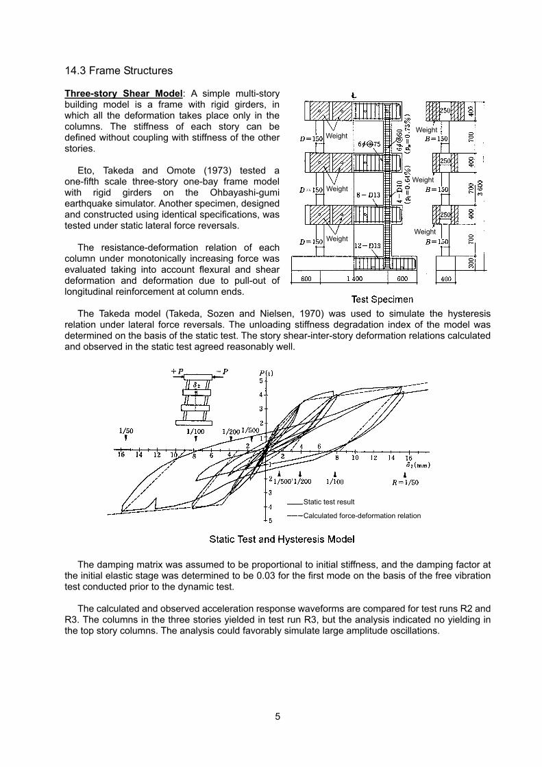
5

14.3 Frame Structures Three-story Shear Model: A simple multi-story building model is a frame with rigid girders, in which all the deformation takes place only in the columns. The stiffness of each story can be defined without coupling with stiffness of the other stories.

Eto, Takeda and Omote (1973) tested a one-fifth scale three-story one-bay frame model with rigid girders on the Ohbayashi-gumi earthquake simulator. Another specimen, designed and constructed using identical specifications, was tested under static lateral force reversals.

The resistance-deformation relation of each column under monotonically increasing force was evaluated taking into account flexural and shear deformation and deformation due to pull-out of longitudinal reinforcement at column ends.

The Takeda model (Takeda, Sozen and Nielsen, 1970) was used to simulate the hysteresis relation under lateral force reversals. The unloading stiffness degradation index of the model was determined on the basis of the static test. The story shear-inter-story deformation relations calculated and observed in the static test agreed reasonably well.

The damping matrix was assumed to be proportional to initial stiffness, and the damping factor at

the initial elastic stage was determined to be 0.03 for the first mode on the basis of the free vibration test conducted prior to the dynamic test.

The calculated and observed acceleration response waveforms are compared for test runs R2 and R3. The columns in the three stories yielded in test run R3, but the analysis indicated no yielding in the top story columns. The analysis could favorably simulate large amplitude oscillations.

Weight

Weight

Weight

Weight

Weight

Weight

Static test result

Calculated force-deformation relation

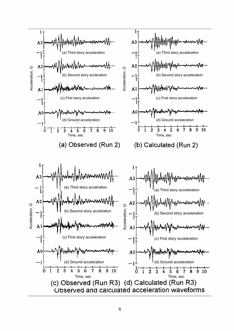
6

(a) Third story acceleration

(b) Second story accleration

(c) First story accleration

(d) Ground acceleration

(a) Third story acceleration

(b) Second story acceleration

(c) First story acceleration

(d) Ground acceleration

Time, sec Time, sec

Acc

eler

atio

n, G

Acc

eler

atio

n, G

(a) Third story accelration

(b) Second story accelration

(c) First story acceleration

(d) Ground acceleration

(a) Third story acceleration

(b) Second story acceleration

(c) First story acceleration

(d) Ground acceleration

Time, sec Time, sec

Acc

eler

atio

n, G

Acc

eler

atio

n, G

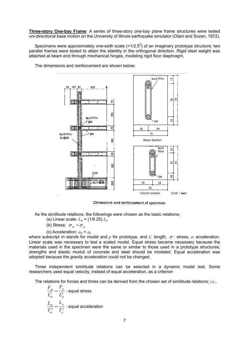
7

Three-story One-bay Frame: A series of three-story one-bay plane frame structures were tested uni-directional base motion on the University of Illinois earthquake simulator (Otani and Sozen, 1972).

Specimens were approximately one-sixth scale (=1/2.52) of an imaginary prototype structure; two parallel frames were tested to attain the stability in the orthogonal direction. Rigid steel weight was attached at beam end through mechanical hinges, modeling rigid floor diaphragm.

The dimensions and reinforcement are shown below;

As the similitude relations, the followings were chosen as the basic relations;

(a) Linear scale: Lm = (1/6.25) Lp (b) Stress: pm σσ = (c) Acceleration: am = ap

where subscript m stands for model and p for prototype, and L: length, σ : stress, a: acceleration. Linear scale was necessary to test a scaled model. Equal stress became necessary because the materials used in the specimen were the same or similar to those used in a prototype structures; strengths and elastic moduli of concrete and steel should be modeled. Equal acceleration was adopted because the gravity acceleration could not be changed.

Three independent similitude relations can be selected in a dynamic model test. Some researchers used equal velocity, instead of equal acceleration, as a criterion

The relations for forces and times can be derived from the chosen set of similitude relations; i.e.,

22p

p

m

m

LF

LF

= : equal stress

22p

p

m

m

TL

TL

= : equal acceleration

Wire

Wire

Wire

Wire

Beam Section

Column section Unit

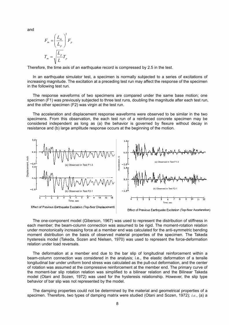
8

and

pp

m

pp

mm

TLL

T

FLL

F

=

=

2

Therefore, the time axis of an earthquake record is compressed by 2.5 in the test.

In an earthquake simulator test, a specimen is normally subjected to a series of excitations of increasing magnitude. The excitation at a preceding test run may affect the response of the specimen in the following test run.

The response waveforms of two specimens are compared under the same base motion; one specimen (F1) was previously subjected to three test runs, doubling the magnitude after each test run, and the other specimen (F2) was virgin at the test run.

The acceleration and displacement response waveforms were observed to be similar in the two specimens. From this observation, the each test run of a reinforced concrete specimen may be considered independent as long as (a) the behavior is governed by flexure without decay in resistance and (b) large amplitude response occurs at the beginning of the motion.

The one-component model (Giberson, 1967) was used to represent the distribution of stiffness in

each member; the beam-column connection was assumed to be rigid. The moment-rotation relation under monotonically increasing force at a member end was calculated for the anti-symmetric bending moment distribution on the basis of observed material properties of the specimen. The Takeda hysteresis model (Takeda, Sozen and Nielsen, 1970) was used to represent the force-deformation relation under load reversals.

The deformation at a member end due to the bar slip of longitudinal reinforcement within a beam-column connection was considered in the analysis; i.e., the elastic deformation of a tensile longitudinal bar under uniform bond stress was calculated as the pull-out deformation, and the center of rotation was assumed at the compressive reinforcement at the member end. The primary curve of the moment-bar slip rotation relation was simplified to a bilinear relation and the Bilinear Takeda model (Otani and Sozen, 1972) was used for the hysteresis relationship. However, the slip type behavior of bar slip was not represented by the model.

The damping properties could not be determined by the material and geometrical properties of a specimen. Therefore, two types of damping matrix were studied (Otani and Sozen, 1972); i.e., (a) a

(a) Observed in Test F1-3

(b) Observed in Test F2-1

Time, sec

Dis

plac

emen

t, in

ch

(a) Observed in Test F1-3

(b) Observed in Test F2-1

Time, sec

Acce

lera

tion,

G

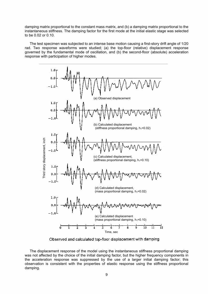
9

damping matrix proportional to the constant mass matrix, and (b) a damping matrix proportional to the instantaneous stiffness. The damping factor for the first mode at the initial elastic stage was selected to be 0.02 or 0.10.

The test specimen was subjected to an intense base motion causing a first-story drift angle of 1/20 rad. Two response waveforms were studied; (a) the top-floor (relative) displacement response governed by the fundamental mode of oscillation, and (b) the second-floor (absolute) acceleration response with participation of higher modes.

The displacement response of the model using the instantaneous stiffness proportional damping

was not affected by the choice of the initial damping factor, but the higher frequency components in the acceleration response was suppressed by the use of a larger initial damping factor; this observation is consistent with the properties of elastic response using the stiffness proportional damping.

(a) Observed displacement

(b) Calculated displacement (stiffness proportional damping, h1=0.02)

(c) Calculated displacement, (stiffness proportional damping, h1=0.10)

(d) Calculated displacement, (mass proportional damping, h1=0.02)

(e) Calculated displacement (mass proportional damping, h1=0.10)

Time, sec

Third

sto

ry d

ispl

acem

ent,

inch

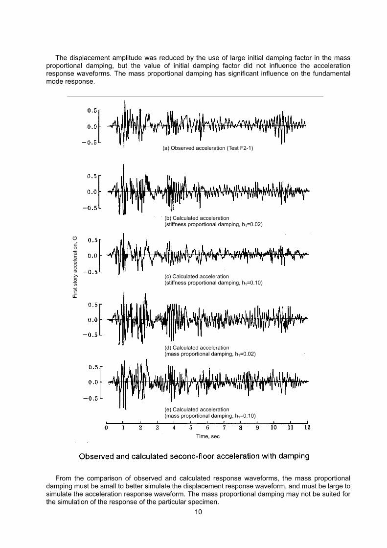
10

The displacement amplitude was reduced by the use of large initial damping factor in the mass

proportional damping, but the value of initial damping factor did not influence the acceleration response waveforms. The mass proportional damping has significant influence on the fundamental mode response.

From the comparison of observed and calculated response waveforms, the mass proportional

damping must be small to better simulate the displacement response waveform, and must be large to simulate the acceleration response waveform. The mass proportional damping may not be suited for the simulation of the response of the particular specimen.

(a) Observed acceleration (Test F2-1)

(b) Calculated acceleration (stiffness proportional damping, h1=0.02)

(c) Calculated acceleration (stiffness proportional damping, h1=0.10)

(d) Calculated acceleration (mass proportional damping, h1=0.02)

(e) Calculated acceleration (mass proportional damping, h1=0.10)

Time, sec

Firs

t sto

ry a

ccel

erat

ion,

G

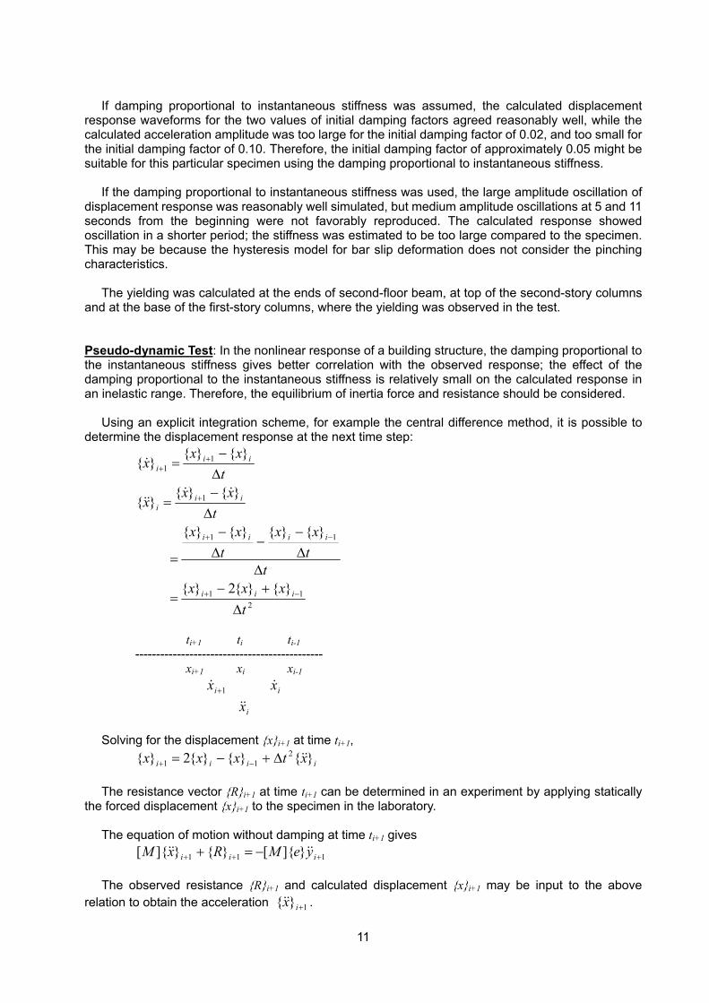
11

If damping proportional to instantaneous stiffness was assumed, the calculated displacement

response waveforms for the two values of initial damping factors agreed reasonably well, while the calculated acceleration amplitude was too large for the initial damping factor of 0.02, and too small for the initial damping factor of 0.10. Therefore, the initial damping factor of approximately 0.05 might be suitable for this particular specimen using the damping proportional to instantaneous stiffness.

If the damping proportional to instantaneous stiffness was used, the large amplitude oscillation of displacement response was reasonably well simulated, but medium amplitude oscillations at 5 and 11 seconds from the beginning were not favorably reproduced. The calculated response showed oscillation in a shorter period; the stiffness was estimated to be too large compared to the specimen. This may be because the hysteresis model for bar slip deformation does not consider the pinching characteristics.

The yielding was calculated at the ends of second-floor beam, at top of the second-story columns and at the base of the first-story columns, where the yielding was observed in the test. Pseudo-dynamic Test: In the nonlinear response of a building structure, the damping proportional to the instantaneous stiffness gives better correlation with the observed response; the effect of the damping proportional to the instantaneous stiffness is relatively small on the calculated response in an inelastic range. Therefore, the equilibrium of inertia force and resistance should be considered.

Using an explicit integration scheme, for example the central difference method, it is possible to determine the displacement response at the next time step:

211

11

1

11

}{}{2}{

}{}{}{}{

}{}{}{

}{}{}{

txxx

ttxx

txx

txx

x

txx

x

iii

iiii

iii

iii

∆+−

=

∆∆−

−∆−

=

∆−

=

∆−

=

−+

−+

+

++

&&&&

&

ti+1 ti ti-1

--------------------------------------------- xi+1 xi xi-1 1+ix& ix&

ix&&

Solving for the displacement {x}i+1 at time ti+1, iiii xtxxx }{}{}{2}{ 2

11 &&∆+−= −+

The resistance vector {R}i+1 at time ti+1 can be determined in an experiment by applying statically the forced displacement {x}i+1 to the specimen in the laboratory.

The equation of motion without damping at time ti+1 gives 111 }]{[}{}]{[ +++ −=+ iii yeMRxM &&&&

The observed resistance {R}i+1 and calculated displacement {x}i+1 may be input to the above relation to obtain the acceleration 1}{ +ix&& .

12

This testing method was called "On-line test" or "Pseudo-dynamic test," originally developed by Dr. M. Hakuno (1969) using an analog computer.

The method has been extensively used in various earthquake response tests (e.g., Okada and Seki, 1979). The major advantages of the test method are that (a) the development of damage in the specimen can be observed and (b) the hysteresis relations need not be assumed in the analysis. The difficulty in the method is to evaluate the numerical stability associated with the accuracy in the instrumentation and the procedure and sequence to apply the forced deformation to a multi-degree-of-freedom system.

Teshigawara (1980) tested two-story one-bay frames. One specimen (specimen FDR-1) was designed to form the beam yielding mechanism and the other specimen (specimen FDR-2) was designed to form the story side-sway mechanism. The beam section was 150x180 mm, and the column section 150x150 mm. The horizontal forces were applied at the mid-span of the beams.

In the analysis, one component model (Giberson, 1967) was used for beams and columns. The

moment-rotation relation was determined by first analyzing the moment-curvature relation of section by the lamina model, and then member end rotation was assumed proportional to the member end curvature for the inflection point at the mid-point of the member. The degrading trilinear model (Fukada, 1969) was used to define the hysteresis relation.

The observed (solid line) and calculated (dashed line) second-floor displacement and first-story shear waveforms are compared. The large amplitude oscillation was successfully reproduced by the model, but calculated small to medium amplitude waveforms shows a shorter response period, indicating the model stiffness was higher than the observed at a low stress level.

Loading Device

Loading device

Loading device

Loading device

Steel

Steel

Steel

Steel

(a) Specimen FDR-1 (b) Specimen FDR-2

Unit

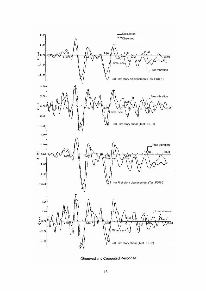
13

CalculatedObserved

(a) First story displacement (Test FDR-1)

(b) First story shear (Test FDR-1)

Time, sec

Free vibration

Free vibration

Time, sec

Free vibration

Time, sec

(c) First story displacement (Test FDR-2)

Free vibration

Time, sec

(d) First story shear (Test FDR-2)

14

References: Clough, R. W., and J. Gidwani, “Reinforced Concrete Frame 2; Seismic Testing and Analytical

Correlation,” EERC Report 76-15, Earthquake Engineering Research Center, University of California at Berkeley, 1976.

Eto, H., T. Takeda and Y. Omote, "Dynamic Destruction Test of Three-story One-span Reinforced Concrete Frames (Part 1: Test Results) (in Japanese)," Report, AIJ Annual Meeting, October 1972, pp. 1119 - 1120, and "ditto, (Part 2: Discussion on Test Results) (in Japanese)," Report, AIJ Kanto District Meeting, 1973, pp. 45 - 48.

Fukada, Y., "Study on the Restoring Force Characteristics of Reinforced Concrete Buildings (in Japanese)," Proceedings, Kanto Branch Symposium, Architectural Institute of Japan, No. 40, 1969, pp. 121-124.

Giberson, M. F., "The Response of Nonlinear Multi-story Structures subjected to Earthquake Excitation," EERL Report, Earthquake Engineering Research Laboratory, California Institute of Technology, Pasadena, 1967.

Hakuno, M., Shidawara, and Hara, "Dynamic Failure Test of Beams Controlled by Computer," Transactions, Japan Society of Civil Engineers, No. 171, November 1969.

Healey, T. J. and M. A. Sozen, “Experimental Study of the Dynamic Response of a Ten-story Reinforced Concrete Frame with a Tall First-story,” Structural Research Series No. 450, Department of Civil Engineering, University of Illinois at Urbana-Champaign, 1978.

Hidalgo, P., and R. W. Clough, “Earthquake Simulator Study of a Reinforced Concrete Frame,” EERC Report 74-13, Earthquake Engineering Research Center, University of California at Berkeley, 1974.

Kabeyasawa, T., H. Shiohara, S. Otani and H. Aoyama, "Analysis of the Full-scale Seven-story Reinforced Concrete Test Structure," Journal, Faculty of Engineering, University of Tokyo (B), Vol. XXXVII, No. 2, 1983, pp. 432-478.

Kunanath, S. K., and A. M. Reinhorn, “Inelastic Three-dimensional Response Analysis of Reinforced Concrete Building Structure (IDARC-3D), Part 1- Modeling,” Technical Report NCEER-89-0011, State University of New York at Buffalo, New York, 1989.

Kunnath, S. K., A. M. Reinhorn, and Y. J. Park, “Analytical Modeling of Inelastic Seismic Response of R/C Structures,“ Proceedings, Journal, Structural Engineering, ASCE, Vol. 116, No. 4, April 1990, pp. 996-10117.

Okada, T., and M. Seki, "Earthquake Response Testing of Reinforced Concrete Frames using Computer-Actuator On-line System, Part 1: Objectives and Methodology (in Japanese)," Transactions, Architectural Institute of Japan, No. 275, January 1979, pp. 25 - 31, "ditto, Part 2: On-line Test 1 (in Japanese)," Transactions, AIJ, No. 279, May 1979, pp. 77 - 84, "ditto, Part 3: On-line Test 2 (in Japanese)," Transactions, AIJ, No. 280, June 1979, pp. 79 - 89, "ditto, Part 4: Discussion of Earthquake Response Characteristics (in Japanese)," Transactions, AIJ, No. 282, August 1979, pp. 57 - 64.

Otani, S., "Earthquake Tests of Shear Wall-Frame Structures to Failure," Proceedings, ASCE/EMD Specialty Conference, University of California at Los Angeles, March 1976, pp. 298 - 307.

Otani, S., and M. A. Sozen, "Behavior of Multistory Reinforced Concrete Frames during Earthquakes," Civil Engineering Studies, SRS No. 392, University of Illinois at Urbana, November 1972.

Otani, S., "Failure Test of Reinforced Concrete Structure, Data for Dynamic Analysis (in Japanese)," Report, AIJ Annual Meeting, September 1980, pp. 1555 - 1556.

Roufail, M. S. L., and C. Meyer, “Analytical Modeling of Hysteretic Behavior of R/C Frames, “Proceedings, ASCE, Journal, Structural Engineering, Vol. 113, No. 3, March 1987, pp. 429-444.

Takeda, T., M. A. Sozen and N. N. Nielsen, "Reinforced Concrete Response to Simulated Earthquakes," Journal, Structural Division, ASCE, Vol. 96, No. ST12, 1970, pp. 2557-2573.

Teshigawara, M., "Simulation of Nonlinear Earthquake Response of Two-story Reinforced Concrete Frames by Computer-Actuator On-line System," M. Eng. Thesis submitted to the University of Tokyo, February 1980.

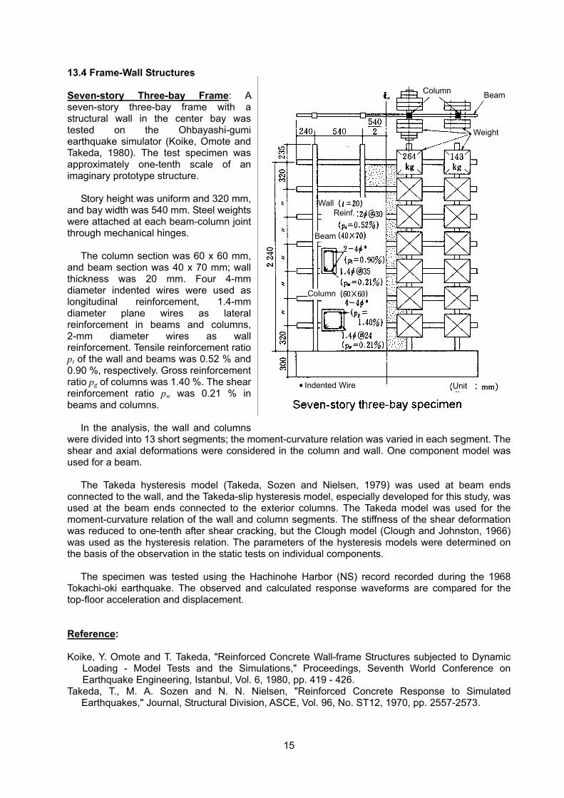
15

13.4 Frame-Wall Structures Seven-story Three-bay Frame: A seven-story three-bay frame with a structural wall in the center bay was tested on the Ohbayashi-gumi earthquake simulator (Koike, Omote and Takeda, 1980). The test specimen was approximately one-tenth scale of an imaginary prototype structure.

Story height was uniform and 320 mm, and bay width was 540 mm. Steel weights were attached at each beam-column joint through mechanical hinges.

The column section was 60 x 60 mm, and beam section was 40 x 70 mm; wall thickness was 20 mm. Four 4-mm diameter indented wires were used as longitudinal reinforcement, 1.4-mm diameter plane wires as lateral reinforcement in beams and columns, 2-mm diameter wires as wall reinforcement. Tensile reinforcement ratio pt of the wall and beams was 0.52 % and 0.90 %, respectively. Gross reinforcement ratio pg of columns was 1.40 %. The shear reinforcement ratio pw was 0.21 % in beams and columns.

In the analysis, the wall and columns were divided into 13 short segments; the moment-curvature relation was varied in each segment. The shear and axial deformations were considered in the column and wall. One component model was used for a beam.

The Takeda hysteresis model (Takeda, Sozen and Nielsen, 1979) was used at beam ends connected to the wall, and the Takeda-slip hysteresis model, especially developed for this study, was used at the beam ends connected to the exterior columns. The Takeda model was used for the moment-curvature relation of the wall and column segments. The stiffness of the shear deformation was reduced to one-tenth after shear cracking, but the Clough model (Clough and Johnston, 1966) was used as the hysteresis relation. The parameters of the hysteresis models were determined on the basis of the observation in the static tests on individual components.

The specimen was tested using the Hachinohe Harbor (NS) record recorded during the 1968 Tokachi-oki earthquake. The observed and calculated response waveforms are compared for the top-floor acceleration and displacement. Reference: Koike, Y. Omote and T. Takeda, "Reinforced Concrete Wall-frame Structures subjected to Dynamic

Loading - Model Tests and the Simulations," Proceedings, Seventh World Conference on Earthquake Engineering, Istanbul, Vol. 6, 1980, pp. 419 - 426.

Takeda, T., M. A. Sozen and N. N. Nielsen, "Reinforced Concrete Response to Simulated Earthquakes," Journal, Structural Division, ASCE, Vol. 96, No. ST12, 1970, pp. 2557-2573.

Weight

Column Beam

Wall Reinf.

Beam

Column

Indented Wire Unit

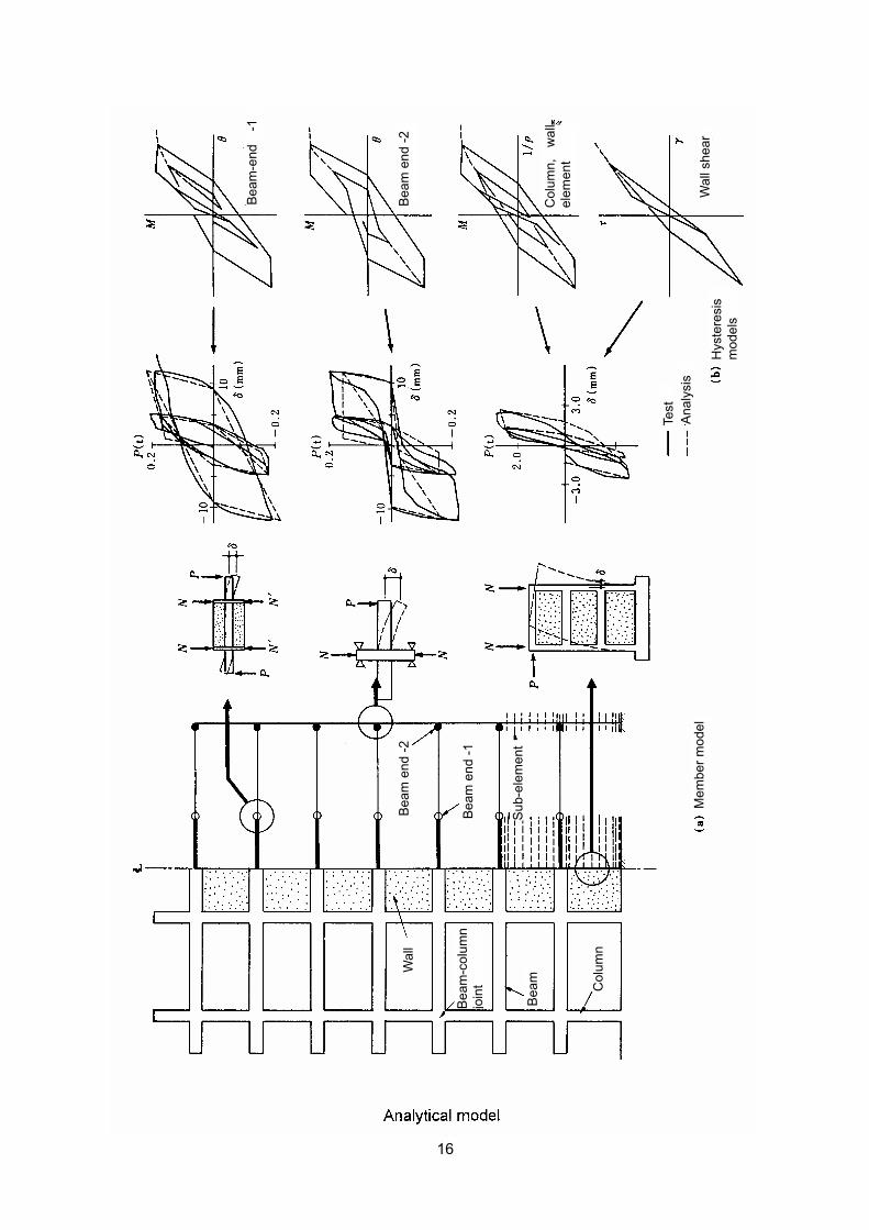
16

Mem

ber m

odel

Bea

m-e

nd

-1

Beam

end

-2

Col

umn,

w

all

elem

ent

Hys

tere

sis

m

odel

s

Test

A

naly

sis

Wal

l she

ar

Beam

end

-2

Beam

end

-1

Sub

-ele

men

t

Wal

l

Bea

m-c

olum

n jo

int

Bea

m

Col

umn

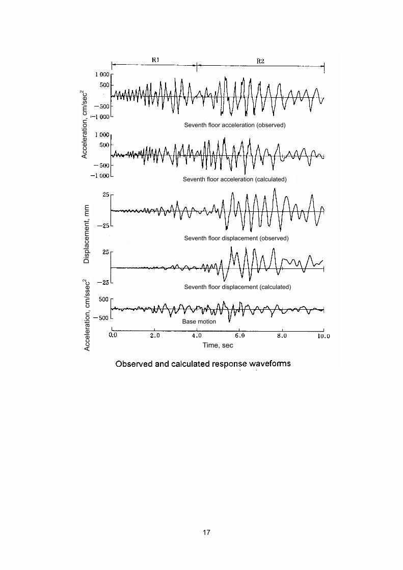
17

Seventh floor acceleration (observed)

Seventh floor acceleration (calculated)

Seventh floor displacement (observed)

Seventh floor displacement (calculated)

Base motion

Time, sec

Acc

eler

atio

n, c

m/s

ec2

Dis

plac

emen

t, m

m

Acc

eler

atio

n, c

m/s

sec2

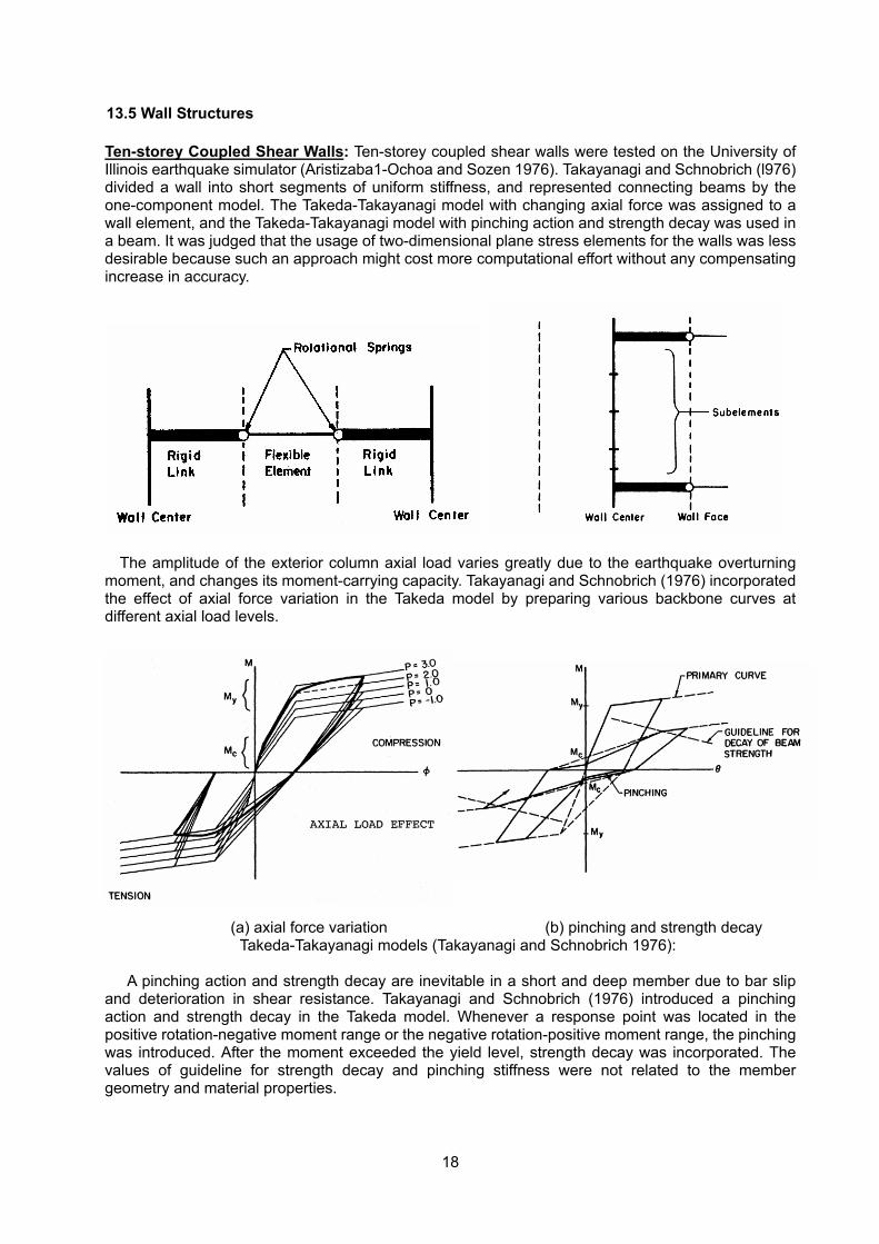
18

13.5 Wall Structures Ten-storey Coupled Shear Walls: Ten-storey coupled shear walls were tested on the University of Illinois earthquake simulator (Aristizaba1-Ochoa and Sozen 1976). Takayanagi and Schnobrich (l976) divided a wall into short segments of uniform stiffness, and represented connecting beams by the one-component model. The Takeda-Takayanagi model with changing axial force was assigned to a wall element, and the Takeda-Takayanagi model with pinching action and strength decay was used in a beam. It was judged that the usage of two-dimensional plane stress elements for the walls was less desirable because such an approach might cost more computational effort without any compensating increase in accuracy.

The amplitude of the exterior column axial load varies greatly due to the earthquake overturning moment, and changes its moment-carrying capacity. Takayanagi and Schnobrich (1976) incorporated the effect of axial force variation in the Takeda model by preparing various backbone curves at different axial load levels.

(a) axial force variation (b) pinching and strength decay Takeda-Takayanagi models (Takayanagi and Schnobrich 1976):

A pinching action and strength decay are inevitable in a short and deep member due to bar slip

and deterioration in shear resistance. Takayanagi and Schnobrich (1976) introduced a pinching action and strength decay in the Takeda model. Whenever a response point was located in the positive rotation-negative moment range or the negative rotation-positive moment range, the pinching was introduced. After the moment exceeded the yield level, strength decay was incorporated. The values of guideline for strength decay and pinching stiffness were not related to the member geometry and material properties.

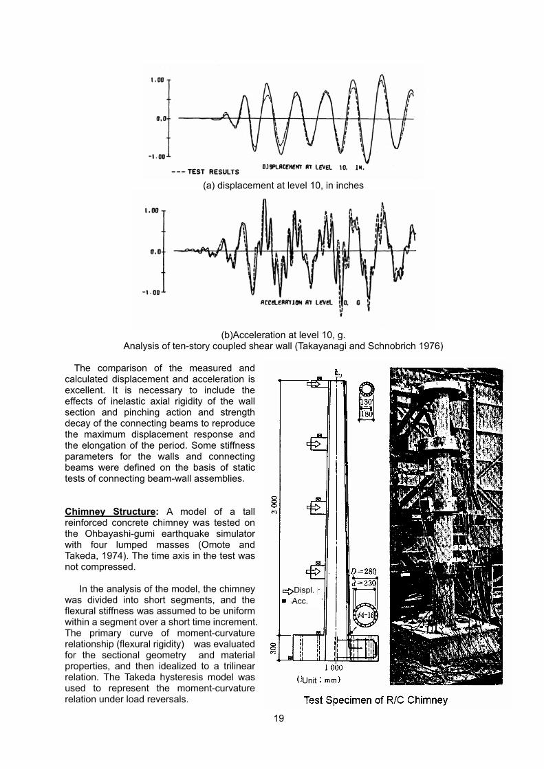
19

(a) displacement at level 10, in inches

(b)Acceleration at level 10, g.

Analysis of ten-story coupled shear wall (Takayanagi and Schnobrich 1976)

The comparison of the measured and calculated displacement and acceleration is excellent. It is necessary to include the effects of inelastic axial rigidity of the wall section and pinching action and strength decay of the connecting beams to reproduce the maximum displacement response and the elongation of the period. Some stiffness parameters for the walls and connecting beams were defined on the basis of static tests of connecting beam-wall assemblies.

Chimney Structure: A model of a tall reinforced concrete chimney was tested on the Ohbayashi-gumi earthquake simulator with four lumped masses (Omote and Takeda, 1974). The time axis in the test was not compressed.

In the analysis of the model, the chimney was divided into short segments, and the flexural stiffness was assumed to be uniform within a segment over a short time increment. The primary curve of moment-curvature relationship (flexural rigidity) was evaluated for the sectional geometry and material properties, and then idealized to a trilinear relation. The Takeda hysteresis model was used to represent the moment-curvature relation under load reversals.

Unit

Displ.Acc.

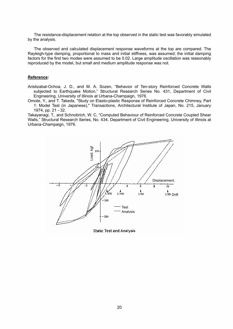
20

The resistance-displacement relation at the top observed in the static test was favorably simulated

by the analysis.

The observed and calculated displacement response waveforms at the top are compared. The Rayleigh-type damping, proportional to mass and initial stiffness, was assumed; the initial damping factors for the first two modes were assumed to be 0.02. Large amplitude oscillation was reasonably reproduced by the model, but small and medium amplitude response was not. Reference: Aristizabal-Ochoa, J. D., and M. A. Sozen, “Behavior of Ten-story Reinforced Concrete Walls

subjected to Earthquake Motion,” Structural Research Series No. 431, Department of Civil Engineering, University of Illinois at Urbana-Champaign, 1976.

Omote, Y., and T. Takeda, "Study on Elasto-plastic Response of Reinforced Concrete Chimney, Part 1: Model Test (in Japanese)," Transactions, Architectural Institute of Japan, No. 215, January 1974, pp. 21 - 32.

Takayanagi, T., and Schnobrich, W. C, “Computed Behaviour of Reinforced Concrete Coupled Shear Walls,” Structural Research Series, No. 434, Department of Civil Engineering, University of Illinois at Urbana-Champaign, 1976.

TestAnalysis

Drift

Displacement,

Load

, kgf

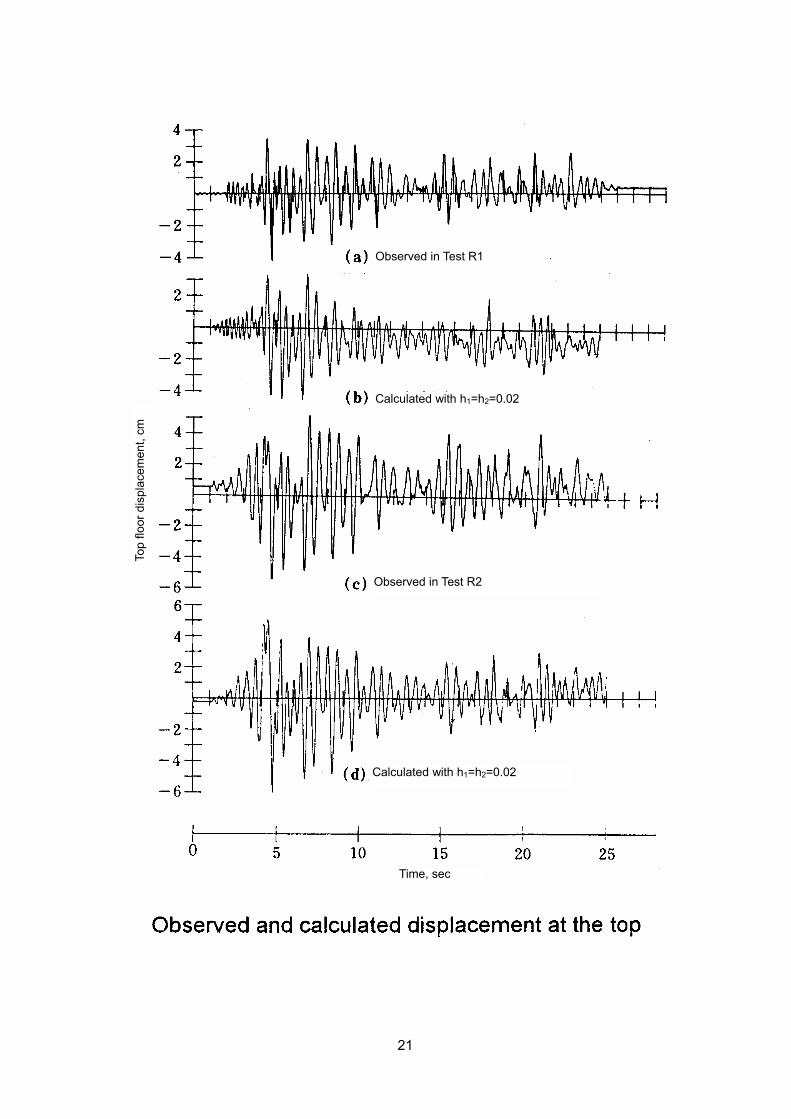
21

Observed in Test R1

Calculated with h1=h2=0.02

Observed in Test R2

Calculated with h1=h2=0.02

Time, sec

Top

floor

dis

plac

emen

t, cm

1

Chapter 15. U.S.-Japan Full-scale Test

This paper describes an analysis of the full-scale seven-story reinforced concrete building tested as a part of the U.S.-Japan Cooperative Research Program Utilizing Large Scale Testing Facilities. A general purpose computer program was developed to simulate the inelastic behavior of a structure during an earthquake. On the basis of given structural geometry and material properties, this paper places an emphasis to describe (a) methods to model member behavior, and (b) methods to determine member stiffness properties. At the time of analysis, the results of small-scale sub-assemblage tests and the full-scale test were made available to the authors, hence, the information was reflected in the development of the analytical models and evaluation methods. A good correlation of the observed and computed responses of the test structure is reported in this paper. 15.1 Test Program of Full-scale Seven-story RC Building

A test of a full-scale reinforced concrete building was conducted, as a part of U.S.-Japan Cooperative Research Program Utilizing Large Scale Testing Facilities, at the Large Size Structures Laboratory of Building Research Institute, Ministry of Construction, Tsukuba, Japan (1).

A full-scale seven-story reinforced concrete building was designed and constructed in the Large

Size Structures Laboratory, Building Research Institute, in accordance with normal construction specifications and practices (Fig. 1). The building had three bays in the longitudinal direction, and two spans in the transverse direction. A shear wall was placed, parallel to the direction of loading, in the middle bay of the center frame.

The structure was subjected to lateral load of an inverted triangular distribution at each level by

eight actuators; two actuators used at the roof level and one actuator each at the other six levels. The pseudo-dynamic test method was used to control the roof-level displacement; i.e., the response displacement under an imaginary earthquake motion was computed, in parallel with the test, for a system having the observed restoring force characteristics. The computed response displacement was applied to the roof level of the test structure while the load amplitude at the first to the sixth floor levels were made proportional to the load measured in the roof level actuators; in this fashion, the number of degrees of freedom of the test structure was reduced to one. A total of 716 channel strains, displacements, rotations and loads were measured during the test.

The intensity of imaginary earthquake motions was varied in four test runs to yield expected

maximum roof-level displacements of approximately 1/7000, 1/400, 3/400, and 1/75 of the total height (Table 1). The earthquake record used in the test was modified from the original record so that the first mode response should dominate in the response of the test structure; i.e., higher frequency components were removed from the original records. Free and forced vibration tests were carried out between pseudo-dynamic earthquake test runs to study the change in period and damping.

After the fourth test run, epoxy resin was injected into major cracks in structural members, and

non-structural partitions were installed to the original bare structure. The repaired structure was tested in three runs using the pseudo-dynamic test method, and finally tested statically under reversals of uniform load distribution to a roof-level displacement of 1/50 the total height.

The second, third and fourth pseudo-dynamic earthquake tests of the bare structure were

simulated by analytical models in this paper.

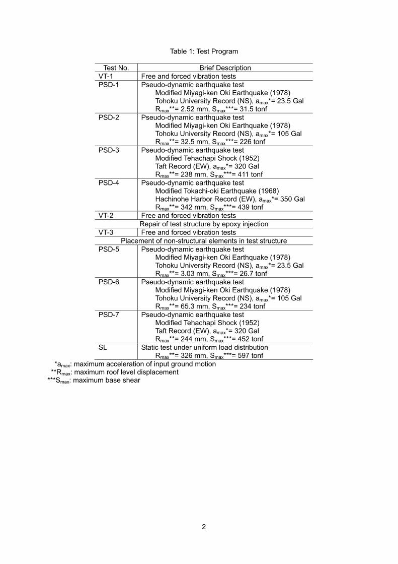
2

Table 1: Test Program

Test No. Brief Description VT-1 Free and forced vibration tests PSD-1 Pseudo-dynamic earthquake test

Modified Miyagi-ken Oki Earthquake (1978) Tohoku University Record (NS), amax*= 23.5 Gal Rmax**= 2.52 mm, Smax***= 31.5 tonf

PSD-2 Pseudo-dynamic earthquake test Modified Miyagi-ken Oki Earthquake (1978) Tohoku University Record (NS), amax*= 105 Gal Rmax**= 32.5 mm, Smax***= 226 tonf

PSD-3 Pseudo-dynamic earthquake test Modified Tehachapi Shock (1952) Taft Record (EW), amax*= 320 Gal Rmax**= 238 mm, Smax***= 411 tonf

PSD-4 Pseudo-dynamic earthquake test Modified Tokachi-oki Earthquake (1968) Hachinohe Harbor Record (EW), amax*= 350 Gal Rmax**= 342 mm, Smax***= 439 tonf

VT-2 Free and forced vibration tests Repair of test structure by epoxy injection

VT-3 Free and forced vibration tests Placement of non-structural elements in test structure

PSD-5 Pseudo-dynamic earthquake test Modified Miyagi-ken Oki Earthquake (1978) Tohoku University Record (NS), amax*= 23.5 Gal Rmax**= 3.03 mm, Smax***= 26.7 tonf

PSD-6 Pseudo-dynamic earthquake test Modified Miyagi-ken Oki Earthquake (1978) Tohoku University Record (NS), amax*= 105 Gal Rmax**= 65.3 mm, Smax***= 234 tonf

PSD-7 Pseudo-dynamic earthquake test Modified Tehachapi Shock (1952) Taft Record (EW), amax*= 320 Gal Rmax**= 244 mm, Smax***= 452 tonf

SL Static test under uniform load distribution Rmax**= 326 mm, Smax***= 597 tonf

*amax: maximum acceleration of input ground motion **Rmax: maximum roof level displacement ***Smax: maximum base shear

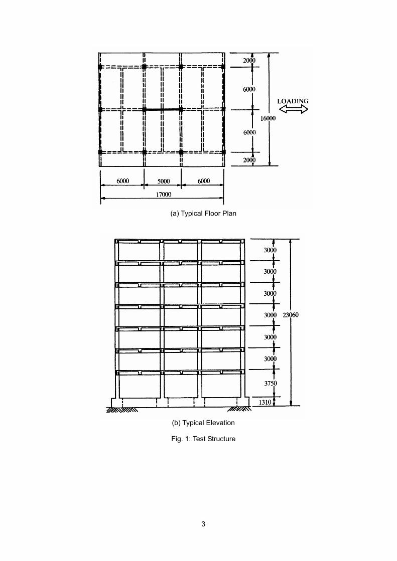
3

(a) Typical Floor Plan

(b) Typical Elevation

Fig. 1: Test Structure

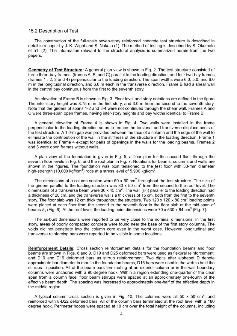
4

15.2 Description of Test The construction of the full-scale seven-story reinforced concrete test structure is described in

detail in a paper by J. K. Wight and S. Nakata (1). The method of testing is described by S. Okamoto et a1. (2). The information relevant to the structural analysis is summarized herein from the two papers.

Geometry of Test Structure: A general plan view is shown in Fig. 2. The test structure consisted of three three-bay frames, (frames A, B, and C) parallel to the loading direction, and four two-bay frames, (frames 1 , 2, 3 and 4) perpendicular to the loading direction. The span widths were 6.0, 5.0, and 6.0 m in the longitudinal direction, and 6.0 m each in the transverse direction. Frame B had a shear wall in the central bay continuous from the first to the seventh story.

An elevation of Frame B is shown in Fig. 3. Floor level and story notations are defined in the figure.

The inter-story height was 3.75 m in the first story, and 3.0 m from the second to the seventh story. Note that the girders of spans 1-2 and 3-4 were not continued through the shear wall. Frames A and C were three-span open frames, having inter-story heights and bay widths identical to Frame B.

A general elevation of Frame 4 is shown in Fig. 4. Two walls were installed in the frame

perpendicular to the loading direction so as to reduce the torsional and transverse displacements of the test structure. A 1.0-m gap was provided between the face of a column and the edge of the wall to eliminate the contribution of the wall in the stiffness of the structure in the loading direction. Frame 1 was identical to Frame 4 except for pairs of openings in the walls for the loading beams. Frames 2 and 3 were open frames without walls.

A plan view of the foundation is given in Fig. 5, a floor plan for the second floor through the

seventh floor levels in Fig. 6, and the roof plan in Fig. 7. Notations for beams, columns and walls are shown in the figures. The foundation was post tensioned to the test floor with 33-mm diameter high-strength (10,000 kgf/cm2) rods at a stress level of 5,900 kgf/cm2.

The dimensions of a column section were 50 x 50 cm2 throughout the test structure. The size of

the girders parallel to the loading direction was 30 x 50 cm2 from the second to the roof level. The dimensions of a transverse beam were 30 x 45 cm2. The wall (W1) parallel to the loading direction had a thickness of 20 cm, and the transverse walls a thickness of 15 cm, both from the first to the seventh story. The floor slab was 12 cm thick throughout the structure. Two 120 x 120 x 80 cm3 loading points were placed at each floor from the second to the seventh floor in the floor slab at the mid-span of beams B2 (Fig. 6). At the roof level, the loading point dimensions were 70 x 530 x 64 cm3 (Fig. 7).

The as-built dimensions were reported to be very close to the nominal dimensions. In the first

story, areas of poorly compacted concrete were found near the base of the first story columns. The voids did not penetrate into the column core even in the worst case. However, longitudinal and transverse reinforcing bars were reported to be visible in some locations.

Reinforcement Details: Cross section reinforcement details for the foundation beams and floor beams are shown in Figs. 8 and 9. D19 and D25 deformed bars were used as flexural reinforcement, and D10 and D19 deformed bars as stirrup reinforcement. Two digits after alphabet D denote approximate bar diameter in mm. In the foundation beams, D16 bars were used in the web to hold the stirrups in position. All of the beam bars terminating at an exterior column or in the wall boundary columns were anchored with a 90-degree hook. Within a region extending one-quarter of the clear span from a column face, floor beam stirrups were spaced at an approximately one-fourth of the effective beam depth. The spacing was increased to approximately one-half of the effective depth in the middle region.

A typical column cross section is given in Fig. 10. The columns were all 50 x 50 cm2, and

reinforced with 8-D22 deformed bars. All of the column bars terminated at the roof level with a 180 degree hook. Perimeter hoops were spaced at 10 cm over the total height of the columns, including

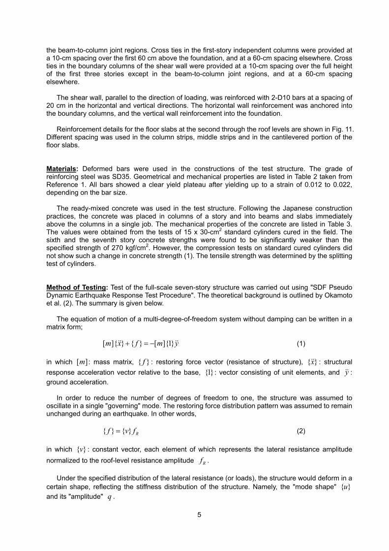
5

the beam-to-column joint regions. Cross ties in the first-story independent columns were provided at a 10-cm spacing over the first 60 cm above the foundation, and at a 60-cm spacing elsewhere. Cross ties in the boundary columns of the shear wall were provided at a 10-cm spacing over the full height of the first three stories except in the beam-to-column joint regions, and at a 60-cm spacing elsewhere.

The shear wall, parallel to the direction of loading, was reinforced with 2-D10 bars at a spacing of

20 cm in the horizontal and vertical directions. The horizontal wall reinforcement was anchored into the boundary columns, and the vertical wall reinforcement into the foundation.

Reinforcement details for the floor slabs at the second through the roof levels are shown in Fig. 11.

Different spacing was used in the column strips, middle strips and in the cantilevered portion of the floor slabs.

Materials: Deformed bars were used in the constructions of the test structure. The grade of reinforcing steel was SD35. Geometrical and mechanical properties are listed in Table 2 taken from Reference 1. All bars showed a clear yield plateau after yielding up to a strain of 0.012 to 0.022, depending on the bar size.

The ready-mixed concrete was used in the test structure. Following the Japanese construction

practices, the concrete was placed in columns of a story and into beams and slabs immediately above the columns in a single job. The mechanical properties of the concrete are listed in Table 3. The values were obtained from the tests of 15 x 30-cm2 standard cylinders cured in the field. The sixth and the seventh story concrete strengths were found to be significantly weaker than the specified strength of 270 kgf/cm2. However, the compression tests on standard cured cylinders did not show such a change in concrete strength (1). The tensile strength was determined by the splitting test of cylinders.

Method of Testing: Test of the full-scale seven-story structure was carried out using "SDF Pseudo Dynamic Earthquake Response Test Procedure". The theoretical background is outlined by Okamoto et al. (2). The summary is given below.

The equation of motion of a multi-degree-of-freedom system without damping can be written in a

matrix form; [ ]{ } { } [ ]{1}m x f m y+ = −&& && (1)

in which [ ]m : mass matrix, { }f : restoring force vector (resistance of structure), { }x&& : structural response acceleration vector relative to the base, {1} : vector consisting of unit elements, and y&& : ground acceleration.

In order to reduce the number of degrees of freedom to one, the structure was assumed to

oscillate in a single "governing" mode. The restoring force distribution pattern was assumed to remain unchanged during an earthquake. In other words,

{ } { } Rf v f= (2)

in which { }v : constant vector, each element of which represents the lateral resistance amplitude normalized to the roof-level resistance amplitude Rf .

Under the specified distribution of the lateral resistance (or loads), the structure would deform in a certain shape, reflecting the stiffness distribution of the structure. Namely, the "mode shape" { }u and its "amplitude" q .

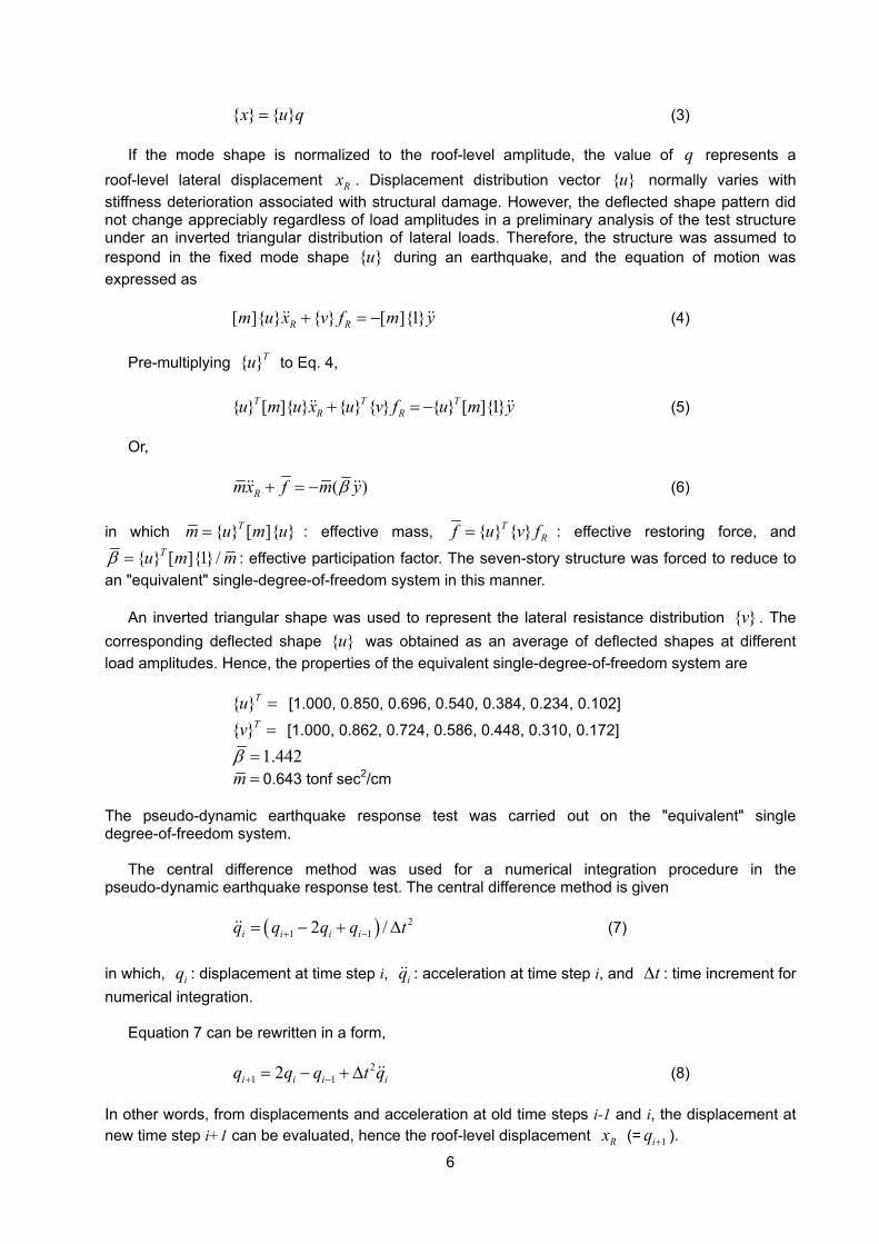
6

{ } { }x u q= (3) If the mode shape is normalized to the roof-level amplitude, the value of q represents a

roof-level lateral displacement Rx . Displacement distribution vector { }u normally varies with stiffness deterioration associated with structural damage. However, the deflected shape pattern did not change appreciably regardless of load amplitudes in a preliminary analysis of the test structure under an inverted triangular distribution of lateral loads. Therefore, the structure was assumed to respond in the fixed mode shape { }u during an earthquake, and the equation of motion was expressed as

[ ]{ } { } [ ]{1}R Rm u x v f m y+ = −&& && (4) Pre-multiplying { }Tu to Eq. 4, { } [ ]{ } { } { } { } [ ]{1}T T T

R Ru m u x u v f u m y+ = −&& && (5) Or, ( )Rmx f m yβ+ = −&& && (6)

in which { } [ ]{ }Tm u m u= : effective mass, { } { }TRf u v f= : effective restoring force, and

{ } [ ]{1}/Tu m mβ = : effective participation factor. The seven-story structure was forced to reduce to an "equivalent" single-degree-of-freedom system in this manner.

An inverted triangular shape was used to represent the lateral resistance distribution { }v . The

corresponding deflected shape { }u was obtained as an average of deflected shapes at different load amplitudes. Hence, the properties of the equivalent single-degree-of-freedom system are

{ }Tu = [1.000, 0.850, 0.696, 0.540, 0.384, 0.234, 0.102]

{ }Tv = [1.000, 0.862, 0.724, 0.586, 0.448, 0.310, 0.172]

1.442β = m = 0.643 tonf sec2/cm

The pseudo-dynamic earthquake response test was carried out on the "equivalent" single degree-of-freedom system.

The central difference method was used for a numerical integration procedure in the pseudo-dynamic earthquake response test. The central difference method is given

( ) 2

1 12 /i i i iq q q q t+ −= − + ∆&& (7)

in which, iq : displacement at time step i, iq&& : acceleration at time step i, and t∆ : time increment for numerical integration.

Equation 7 can be rewritten in a form, 2

1 12i i i iq q q t q+ −= − + ∆ && (8)

In other words, from displacements and acceleration at old time steps i-1 and i, the displacement at new time step i+1 can be evaluated, hence the roof-level displacement Rx (= 1iq + ).

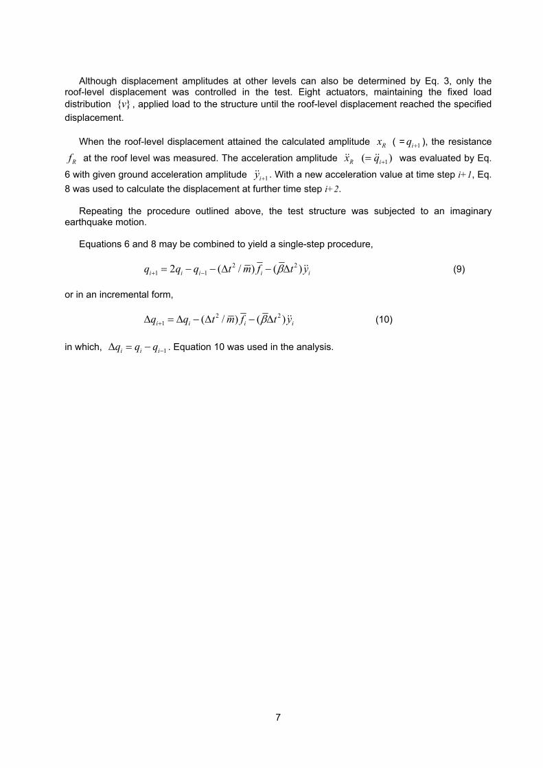
7

Although displacement amplitudes at other levels can also be determined by Eq. 3, only the

roof-level displacement was controlled in the test. Eight actuators, maintaining the fixed load distribution { }v , applied load to the structure until the roof-level displacement reached the specified displacement.

When the roof-level displacement attained the calculated amplitude Rx ( = 1iq + ), the resistance

Rf at the roof level was measured. The acceleration amplitude Rx&& 1( )iq += && was evaluated by Eq.

6 with given ground acceleration amplitude 1iy +&& . With a new acceleration value at time step i+1, Eq. 8 was used to calculate the displacement at further time step i+2.

Repeating the procedure outlined above, the test structure was subjected to an imaginary

earthquake motion. Equations 6 and 8 may be combined to yield a single-step procedure, 2 2

1 12 ( / ) ( )i i i i iq q q t m f t yβ+ −= − − ∆ − ∆ && (9)

or in an incremental form, 2 2

1 ( / ) ( )i i i iq q t m f t yβ+∆ = ∆ − ∆ − ∆ && (10)

in which, 1i i iq q q −∆ = − . Equation 10 was used in the analysis.

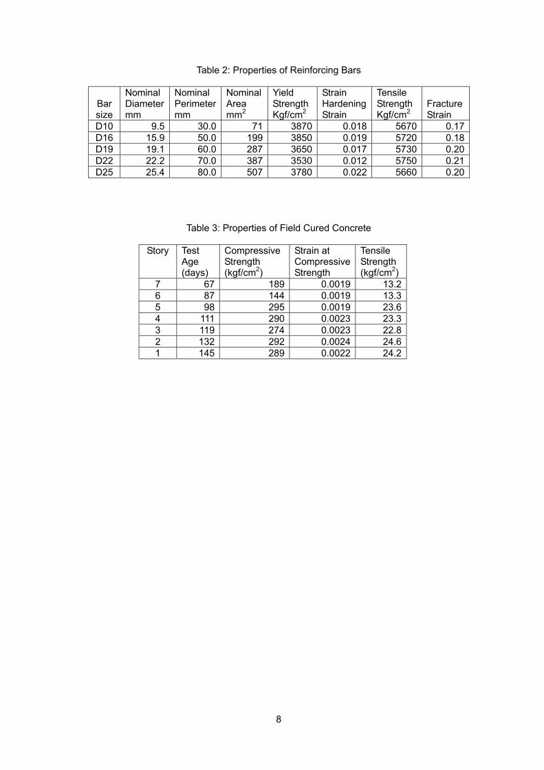
8

Table 2: Properties of Reinforcing Bars

Bar size

Nominal Diametermm

Nominal Perimeter mm

NominalArea mm2

Yield Strength Kgf/cm2

Strain HardeningStrain

Tensile Strength Kgf/cm2

FractureStrain

D10 9.5 30.0 71 3870 0.018 5670 0.17D16 15.9 50.0 199 3850 0.019 5720 0.18D19 19.1 60.0 287 3650 0.017 5730 0.20D22 22.2 70.0 387 3530 0.012 5750 0.21D25 25.4 80.0 507 3780 0.022 5660 0.20

Table 3: Properties of Field Cured Concrete

Story Test Age (days)

Compressive Strength (kgf/cm2)

Strain at CompressiveStrength

Tensile Strength (kgf/cm2)

7 67 189 0.0019 13.2 6 87 144 0.0019 13.3 5 98 295 0.0019 23.6 4 111 290 0.0023 23.3 3 119 274 0.0023 22.8 2 132 292 0.0024 24.6 1 145 289 0.0022 24.2

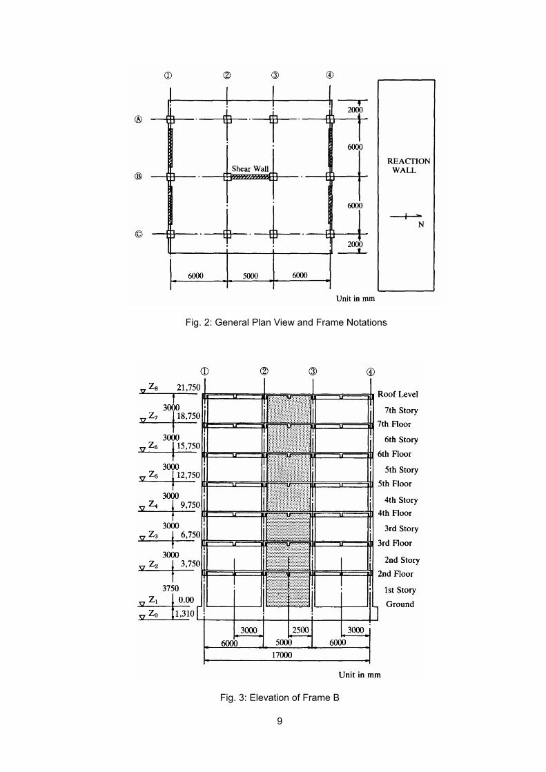
9

Fig. 2: General Plan View and Frame Notations

Fig. 3: Elevation of Frame B

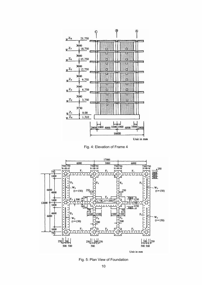
10

Fig. 4: Elevation of Frame 4

Fig. 5: Plan View of Foundation

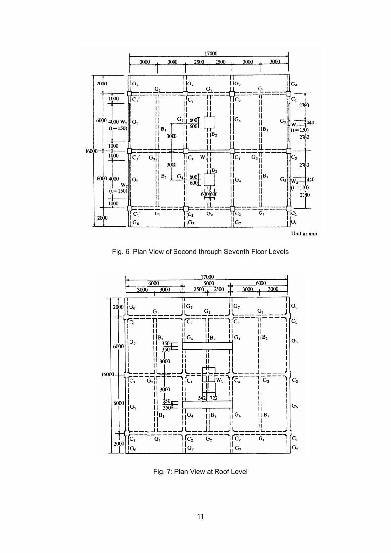
11

Fig. 6: Plan View of Second through Seventh Floor Levels

Fig. 7: Plan View at Roof Level

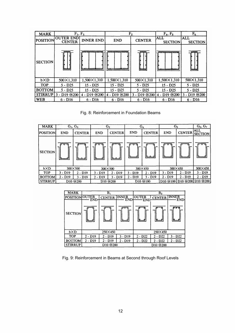
12

Fig. 8: Reinforcement in Foundation Beams

Fig. 9: Reinforcement in Beams at Second through Roof Levels

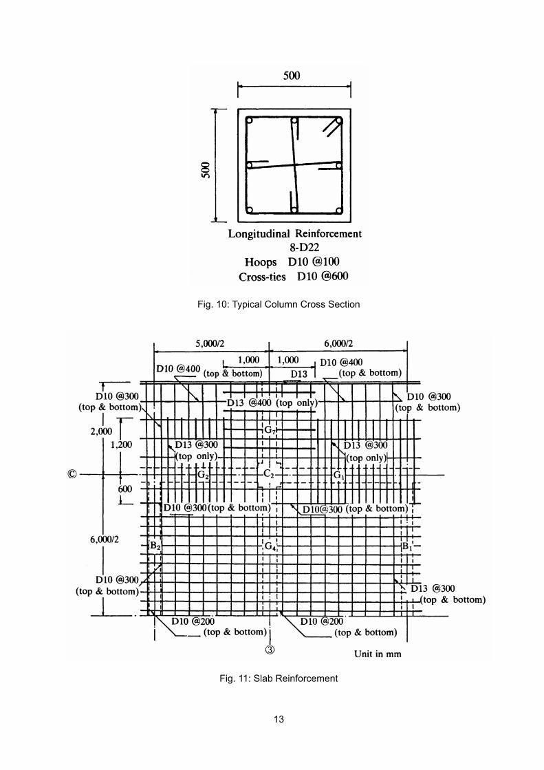
13

Fig. 10: Typical Column Cross Section

Fig. 11: Slab Reinforcement

14

15.3 Modeling of Structural Members It is not feasible to analyze an entire structure using microscopic material models. Therefore, it is

necessary to develop a simple analytical model of structural members. Nonlinear dynamic analysis of a reinforced concrete structure requires two types of mathematical

modeling: (a) modeling for the distribution of stiffness along a member; and (b) modeling for the force-deformation relationship under stress reversals. The former models are called "member models", and the latter "hysteresis models".

Inelastic deformation of a reinforced concrete member does not concentrate in a critical location,

but rather spreads along the member. Various member models have been proposed to represent the distribution of stiffness within a reinforced concrete member (3, 4).

The member models used to represent the stiffness behavior of beams, columns, and walls are

presented in this part.

Beam and Column Model: Many member models have been proposed for the beam and column members; for example, (a) One-component model (5), (b) Multi-component model (6), (c) Connected two-cantilever model (7), (d) Distributed flexibility model (8).

The One-component model was used for beams and columns in this paper. Namely, beam or

column member was idealized as a perfectly elastic massless line element with two nonlinear rotational springs at the two ends. The model could have two rigid zones outside the rotational springs as shown in Fig. 12. Axial deformation is considered in the elastic element of a column member.

The stiffness properties of a rotational spring are evaluated for an imaginary anti-symmetric

loading conditions with the inflection point at the center of the flexible portion of a member. The rotation at a flexible end less the elastic rotation is assigned to the rotational spring. The shear deformation within a member and the member end rotation due to bar slip within the beam-to-column connection should be considered in the evaluation of the deformation.

The shear deformation of a beam-to-column connection panel is not considered in the analysis.

Wall Model: A shear wall is normally idealized as (a) an equivalent column taking flexural and shear deformation into account, (b) a braced frame, in which the shear deformation is represented by the deformation of diagonal elements, whereas the flexural deformation by the deformation of vertical elements, and (c) short line segments along the height with each short segment with hysteretic characteristics (9, 10). These models have advantages and disadvantages. In most cases, the horizontal boundary beams (or slabs) are assumed to be rigid.

The Japanese support tests on three-story walls with connecting beams (11) indicated a large

elongation of a tension-side column due to cracking, and a small compression of the compression-side column, with the neutral axis of wall section close to the compression-side column. In other words, the bending deformation of a wall was caused primarily by the extension of the tension-side boundary column. The resistance of a wall came from the resistances of the boundary columns and that of the central wall section.

The wall member of a story was, therefore, idealized as three vertical line elements with infinitely

rigid beams at the top and bottom floor levels (Fig. 13). Two outside truss elements represented the axial stiffness of boundary columns. The axial stiffness varied with the sign and level of axial stress, and degraded with tensile stress history. The central vertical element was a one-component model in which vertical, horizontal and rotational springs were concentrated at the base. A finite rigid zone could be placed between the spring assembly and the lower rigid chord.

15

The model was intended to simulate the wall deformation under uniform bending, the resistance of wall section being lumped at the locations of the outer truss elements and the central vertical spring. The effect of strain gradient across the wall section was represented by the rotational spring in the central element, and the shear deformation expressed by the deformation of the horizontal spring.

The stiffness matrix of a wall element was formulated as the sum of the stiffness of the three

vertical elements evaluated at the top and bottom of the two boundary columns.

Transverse Beam Model: The tensile boundary column of a wall tends to elongate extensively under bending deformation, yielding a significant vertical displacement at a beam-to-wall-joint node, whereas the vertical displacement of a beam-to-column-joint node of an open frame is relatively small. Consequently, the transverse beam connecting the boundary column of a shear wall and an adjacent parallel open frame is subjected to vertical differential displacement at the two ends, and resists the upward movement of a wall boundary column.

Vertical spring elements, therefore, were introduced to reflect the effect of such transverse beams

to restrain the elongation of a tensile boundary column (Fig. 14). A spring was placed between the joints of the wall and an open frame connected by a transverse beam.

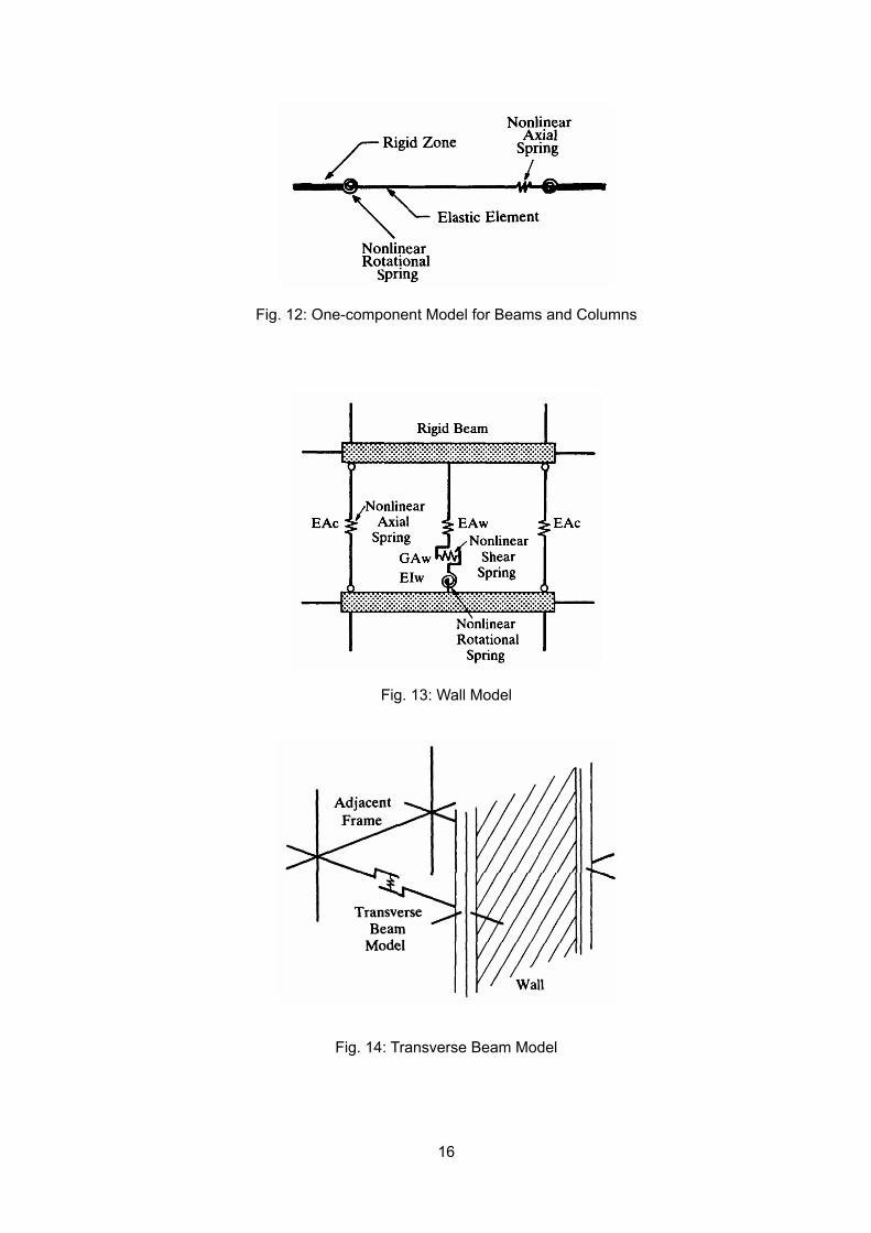
16

Fig. 12: One-component Model for Beams and Columns

Fig. 13: Wall Model

Fig. 14: Transverse Beam Model

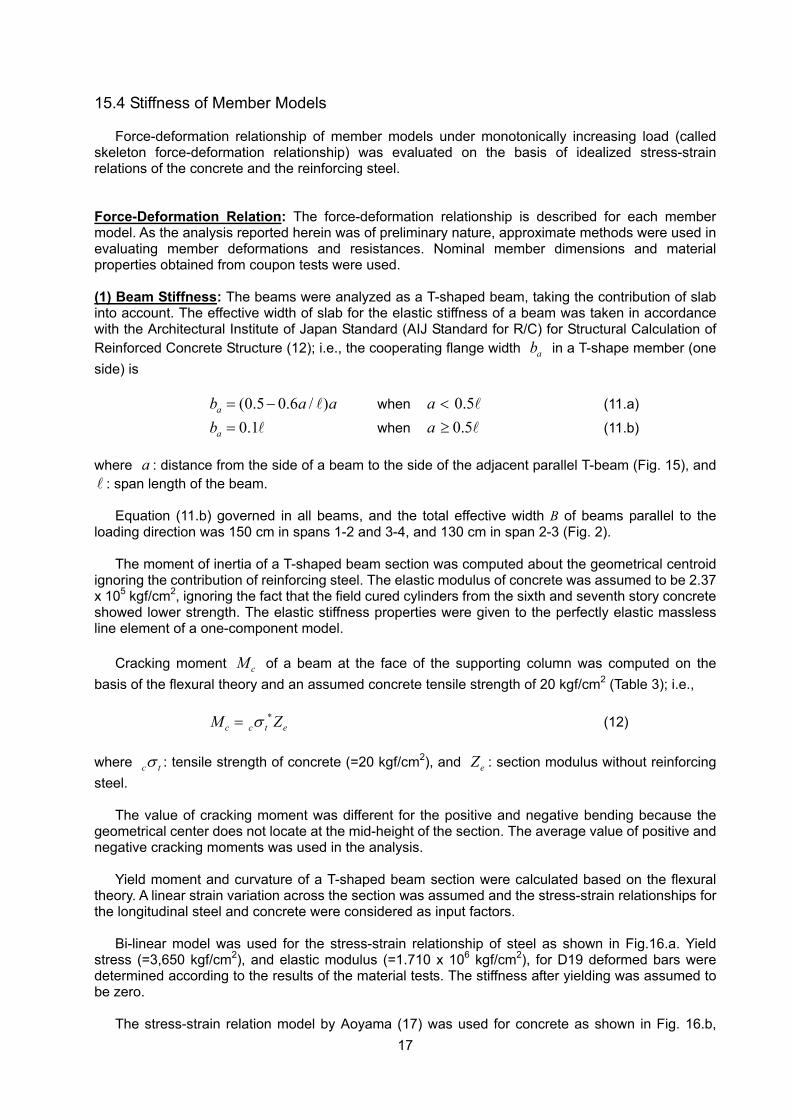
17

15.4 Stiffness of Member Models Force-deformation relationship of member models under monotonically increasing load (called

skeleton force-deformation relationship) was evaluated on the basis of idealized stress-strain relations of the concrete and the reinforcing steel.

Force-Deformation Relation: The force-deformation relationship is described for each member model. As the analysis reported herein was of preliminary nature, approximate methods were used in evaluating member deformations and resistances. Nominal member dimensions and material properties obtained from coupon tests were used.

(1) Beam Stiffness: The beams were analyzed as a T-shaped beam, taking the contribution of slab into account. The effective width of slab for the elastic stiffness of a beam was taken in accordance with the Architectural Institute of Japan Standard (AIJ Standard for R/C) for Structural Calculation of Reinforced Concrete Structure (12); i.e., the cooperating flange width ab in a T-shape member (one side) is

(0.5 0.6 / )ab a a= − l when 0.5a < l (11.a)

0.1ab = l when 0.5a ≥ l (11.b)

where a : distance from the side of a beam to the side of the adjacent parallel T-beam (Fig. 15), and l : span length of the beam.

Equation (11.b) governed in all beams, and the total effective width B of beams parallel to the

loading direction was 150 cm in spans 1-2 and 3-4, and 130 cm in span 2-3 (Fig. 2). The moment of inertia of a T-shaped beam section was computed about the geometrical centroid

ignoring the contribution of reinforcing steel. The elastic modulus of concrete was assumed to be 2.37 x 105 kgf/cm2, ignoring the fact that the field cured cylinders from the sixth and seventh story concrete showed lower strength. The elastic stiffness properties were given to the perfectly elastic massless line element of a one-component model.

Cracking moment cM of a beam at the face of the supporting column was computed on the

basis of the flexural theory and an assumed concrete tensile strength of 20 kgf/cm2 (Table 3); i.e., c c t eM Zσ ∗= (12)

where c tσ : tensile strength of concrete (=20 kgf/cm2), and eZ : section modulus without reinforcing steel.

The value of cracking moment was different for the positive and negative bending because the geometrical center does not locate at the mid-height of the section. The average value of positive and negative cracking moments was used in the analysis.

Yield moment and curvature of a T-shaped beam section were calculated based on the flexural

theory. A linear strain variation across the section was assumed and the stress-strain relationships for the longitudinal steel and concrete were considered as input factors.

Bi-linear model was used for the stress-strain relationship of steel as shown in Fig.16.a. Yield

stress (=3,650 kgf/cm2), and elastic modulus (=1.710 x 106 kgf/cm2), for D19 deformed bars were determined according to the results of the material tests. The stiffness after yielding was assumed to be zero.

The stress-strain relation model by Aoyama (17) was used for concrete as shown in Fig. 16.b,

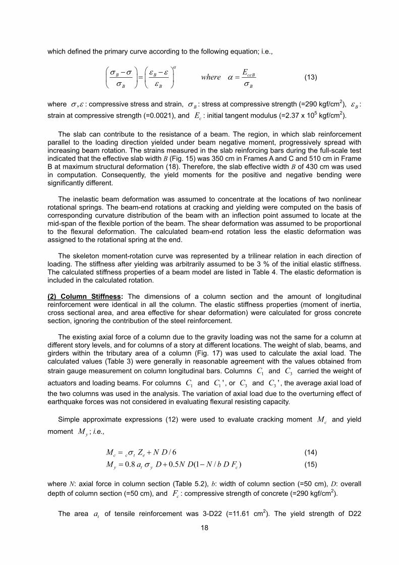
18

which defined the primary curve according to the following equation; i.e.,

c BB B

B B B

Ewhereα

εσ σ ε ε ασ ε σ

− −= =

(13)

where ,σ ε : compressive stress and strain, Bσ : stress at compressive strength (=290 kgf/cm2), Bε : strain at compressive strength (=0.0021), and cE : initial tangent modulus (=2.37 x 105 kgf/cm2).

The slab can contribute to the resistance of a beam. The region, in which slab reinforcement parallel to the loading direction yielded under beam negative moment, progressively spread with increasing beam rotation. The strains measured in the slab reinforcing bars during the full-scale test indicated that the effective slab width B (Fig. 15) was 350 cm in Frames A and C and 510 cm in Frame B at maximum structural deformation (18). Therefore, the slab effective width B of 430 cm was used in computation. Consequently, the yield moments for the positive and negative bending were significantly different.

The inelastic beam deformation was assumed to concentrate at the locations of two nonlinear

rotational springs. The beam-end rotations at cracking and yielding were computed on the basis of corresponding curvature distribution of the beam with an inflection point assumed to locate at the mid-span of the flexible portion of the beam. The shear deformation was assumed to be proportional to the flexural deformation. The calculated beam-end rotation less the elastic deformation was assigned to the rotational spring at the end.

The skeleton moment-rotation curve was represented by a trilinear relation in each direction of

loading. The stiffness after yielding was arbitrarily assumed to be 3 % of the initial elastic stiffness. The calculated stiffness properties of a beam model are listed in Table 4. The elastic deformation is included in the calculated rotation.

(2) Column Stiffness: The dimensions of a column section and the amount of longitudinal reinforcement were identical in all the column. The elastic stiffness properties (moment of inertia, cross sectional area, and area effective for shear deformation) were calculated for gross concrete section, ignoring the contribution of the steel reinforcement.

The existing axial force of a column due to the gravity loading was not the same for a column at different story levels, and for columns of a story at different locations. The weight of slab, beams, and girders within the tributary area of a column (Fig. 17) was used to calculate the axial load. The calculated values (Table 3) were generally in reasonable agreement with the values obtained from strain gauge measurement on column longitudinal bars. Columns 1C and 3C carried the weight of

actuators and loading beams. For columns 1C and 1 'C , or 3C and 3 'C , the average axial load of the two columns was used in the analysis. The variation of axial load due to the overturning effect of earthquake forces was not considered in evaluating flexural resisting capacity.

Simple approximate expressions (12) were used to evaluate cracking moment cM and yield

moment yM ; i.e., / 6c c t eM Z N Dσ= + (14)

0.8 0.5 (1 / )y t y cM a D N D N b D Fσ= + − (15)

where N: axial force in column section (Table 5.2), b: width of column section (=50 cm), D: overall depth of column section (=50 cm), and cF : compressive strength of concrete (=290 kgf/cm2).

The area ta of tensile reinforcement was 3-D22 (=11.61 cm2). The yield strength of D22

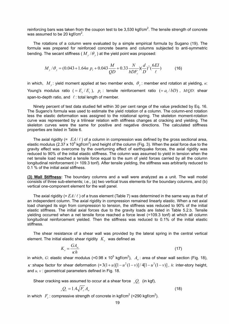
19

reinforcing bars was taken from the coupon test to be 3,530 kgf/cm2. The tensile strength of concrete was assumed to be 20 kgf/cm2.

The rotations of a column were evaluated by a simple empirical formula by Sugano (19). The

formula was prepared for reinforced concrete beams and columns subjected to anti-symmetric bending. The secant stiffness ( /y yM θ ) at the yield point was proposed:

2 6/ (0.043 1.64 0.043 0.33 )( ) ( )y y tc

M N d EIM n pQD bDF D

θ = + + +l

(16)

in which, yM : yield moment applied at two member ends, yθ : member end rotation at yielding, n:

Young's modulus ratio ( /s cE E= ), tp : tensile reinforcement ratio ( / )ta bD= , M/QD: shear span-to-depth ratio, and l : total length of member.

Ninety percent of test data studied fell within 30 per cent range of the value predicted by Eq. 16.

The Sugano's formula was used to estimate the yield rotation of a column. The column-end rotation less the elastic deformation was assigned to the rotational spring. The skeleton moment-rotation curve was represented by a trilinear relation with stiffness changes at cracking and yielding. The skeleton curves were the same for positive and negative directions. The calculated stiffness properties are listed in Table 6.

The axial rigidity (= /EA l ) of a column in compression was defined by the gross sectional area,

elastic modulus (2.37 x 105 kgf/cm2) and height of the column (Fig. 3). When the axial force due to the gravity effect was overcome by the overturning effect of earthquake forces, the axial rigidity was reduced to 90% of the initial elastic stiffness. The column was assumed to yield in tension when the net tensile load reached a tensile force equal to the sum of yield forces carried by all the column longitudinal reinforcement (= 109.3 tonf). After tensile yielding, the stiffness was arbitrarily reduced to 0.1 % of the initial axial stiffness.

(3) Wall Stiffness: The boundary columns and a wall were analyzed as a unit. The wall model consists of three sub-elements; i.e., (a) two vertical truss elements for the boundary columns, and (b) vertical one-component element for the wall panel.

The axial rigidity (= /EA l ) of a truss element (Table 7) was determined in the same way as that of an independent column. The axial rigidity in compression remained linearly elastic. When a net axial load changed its sign from compression to tension, the stiffness was reduced to 90% of the initial elastic stiffness. The initial axial forces due to the gravity loads are listed in Table 5.2.b. Tensile yielding occurred when a net tensile force reached a force level (=109.3 tonf) at which all column longitudinal reinforcement yielded. Then the stiffness was reduced to 0.1% of the initial elastic stiffness.

The shear resistance of a shear wall was provided by the lateral spring in the central vertical

element. The initial elastic shear rigidity sK was defined as

ws

GAKhκ

= (17)

in which, G: elastic shear modulus (=0.98 x 105 kgf/cm2), wA : area of shear wall section (Fig. 18),

κ :shape factor for shear deformation (= 2 33(1 )[1 (1 )] / 4[1 (1 )]u u v u v+ − − − − , h: inter-story height, and u, v : geometrical parameters defined in Fig. 18.

Shear cracking was assumed to occur at a shear force s cQ (in kgf),

1.4s c c wQ F A= (18)

in which cF : compressive strength of concrete in kgf/cm2 (=290 kgf/cm2).

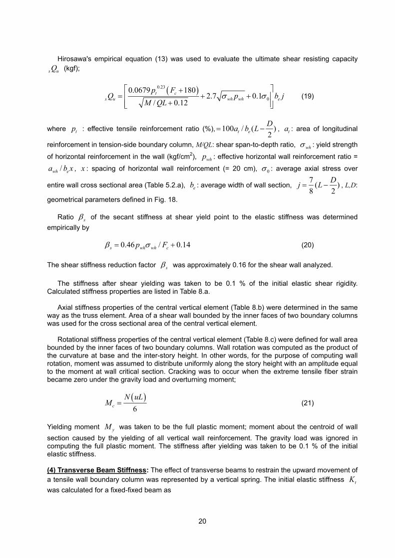
20

Hirosawa's empirical equation (13) was used to evaluate the ultimate shear resisting capacity

s uQ (kgf);

( )0.23

0

0.0679 1802.7 0.1

/ 0.12t c

s u wh wh e

p FQ p b j

M QLσ σ

+= + +

+ (19)

where tp : effective tensile reinforcement ratio (%), 100 / ( )2t eDa b L= − , ta : area of longitudinal

reinforcement in tension-side boundary column, M/QL: shear span-to-depth ratio, whσ : yield strength

of horizontal reinforcement in the wall (kgf/cm2), whp : effective horizontal wall reinforcement ratio =

/wh ea b x , x : spacing of horizontal wall reinforcement (= 20 cm), 0σ : average axial stress over

entire wall cross sectional area (Table 5.2.a), eb : average width of wall section, 7 ( )8 2

Dj L= − , L,D:

geometrical parameters defined in Fig. 18. Ratio sβ of the secant stiffness at shear yield point to the elastic stiffness was determined

empirically by 0.46 / 0.14s wh wh cp Fβ σ= + (20)

The shear stiffness reduction factor sβ was approximately 0.16 for the shear wall analyzed.

The stiffness after shear yielding was taken to be 0.1 % of the initial elastic shear rigidity. Calculated stiffness properties are listed in Table 8.a.

Axial stiffness properties of the central vertical element (Table 8.b) were determined in the same

way as the truss element. Area of a shear wall bounded by the inner faces of two boundary columns was used for the cross sectional area of the central vertical element.

Rotational stiffness properties of the central vertical element (Table 8.c) were defined for wall area

bounded by the inner faces of two boundary columns. Wall rotation was computed as the product of the curvature at base and the inter-story height. In other words, for the purpose of computing wall rotation, moment was assumed to distribute uniformly along the story height with an amplitude equal to the moment at wall critical section. Cracking was to occur when the extreme tensile fiber strain became zero under the gravity load and overturning moment;

( )6c

N uLM = (21)

Yielding moment yM was taken to be the full plastic moment; moment about the centroid of wall section caused by the yielding of all vertical wall reinforcement. The gravity load was ignored in computing the full plastic moment. The stiffness after yielding was taken to be 0.1 % of the initial elastic stiffness.

(4) Transverse Beam Stiffness: The effect of transverse beams to restrain the upward movement of a tensile wall boundary column was represented by a vertical spring. The initial elastic stiffness tK was calculated for a fixed-fixed beam as

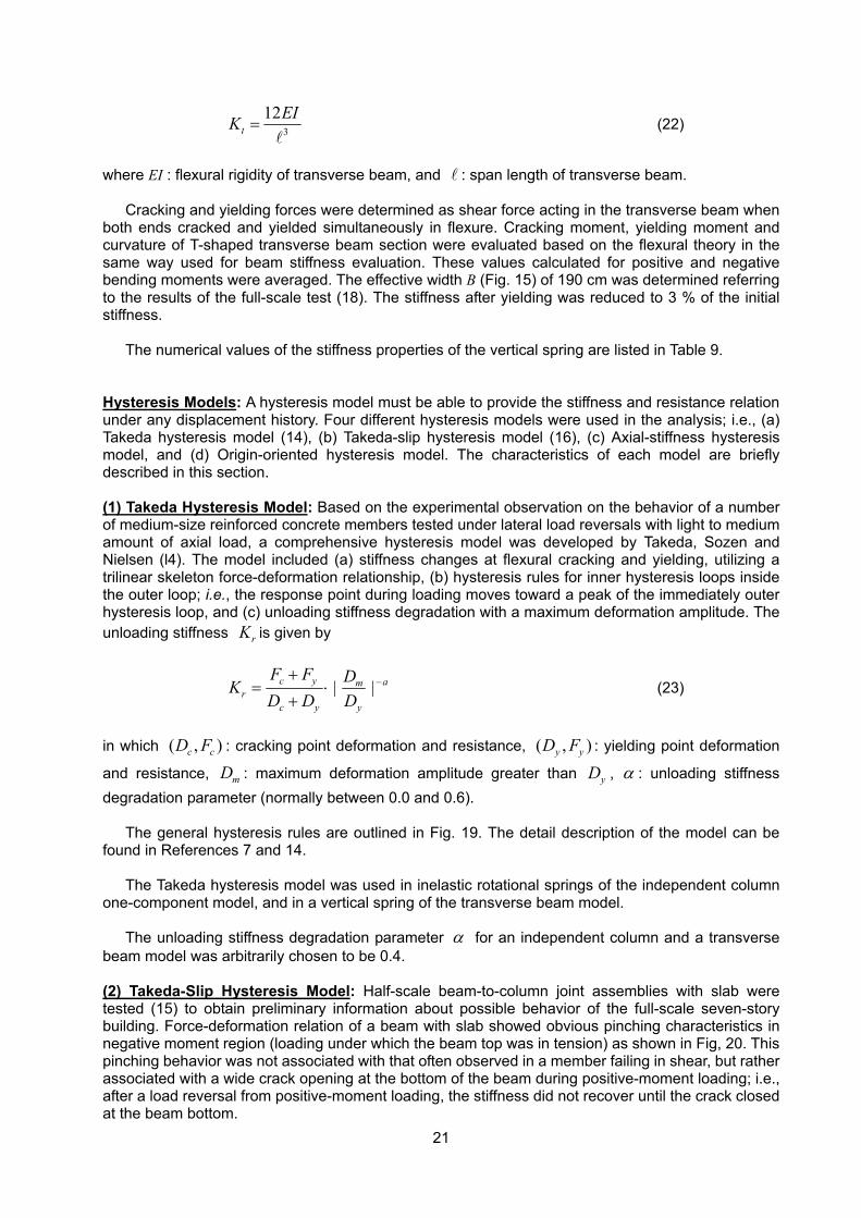
21

3

12t

EIK =l

(22)

where EI : flexural rigidity of transverse beam, and l : span length of transverse beam.

Cracking and yielding forces were determined as shear force acting in the transverse beam when both ends cracked and yielded simultaneously in flexure. Cracking moment, yielding moment and curvature of T-shaped transverse beam section were evaluated based on the flexural theory in the same way used for beam stiffness evaluation. These values calculated for positive and negative bending moments were averaged. The effective width B (Fig. 15) of 190 cm was determined referring to the results of the full-scale test (18). The stiffness after yielding was reduced to 3 % of the initial stiffness.

The numerical values of the stiffness properties of the vertical spring are listed in Table 9.

Hysteresis Models: A hysteresis model must be able to provide the stiffness and resistance relation under any displacement history. Four different hysteresis models were used in the analysis; i.e., (a) Takeda hysteresis model (14), (b) Takeda-slip hysteresis model (16), (c) Axial-stiffness hysteresis model, and (d) Origin-oriented hysteresis model. The characteristics of each model are briefly described in this section.

(1) Takeda Hysteresis Model: Based on the experimental observation on the behavior of a number of medium-size reinforced concrete members tested under lateral load reversals with light to medium amount of axial load, a comprehensive hysteresis model was developed by Takeda, Sozen and Nielsen (l4). The model included (a) stiffness changes at flexural cracking and yielding, utilizing a trilinear skeleton force-deformation relationship, (b) hysteresis rules for inner hysteresis loops inside the outer loop; i.e., the response point during loading moves toward a peak of the immediately outer hysteresis loop, and (c) unloading stiffness degradation with a maximum deformation amplitude. The unloading stiffness rK is given by

| |c y amr

c y y

F F DKD D D

−+= ⋅

+ (23)

in which ( , )c cD F : cracking point deformation and resistance, ( , )y yD F : yielding point deformation

and resistance, mD : maximum deformation amplitude greater than yD , α : unloading stiffness degradation parameter (normally between 0.0 and 0.6).

The general hysteresis rules are outlined in Fig. 19. The detail description of the model can be

found in References 7 and 14. The Takeda hysteresis model was used in inelastic rotational springs of the independent column

one-component model, and in a vertical spring of the transverse beam model. The unloading stiffness degradation parameter α for an independent column and a transverse

beam model was arbitrarily chosen to be 0.4.

(2) Takeda-Slip Hysteresis Model: Half-scale beam-to-column joint assemblies with slab were tested (15) to obtain preliminary information about possible behavior of the full-scale seven-story building. Force-deformation relation of a beam with slab showed obvious pinching characteristics in negative moment region (loading under which the beam top was in tension) as shown in Fig, 20. This pinching behavior was not associated with that often observed in a member failing in shear, but rather associated with a wide crack opening at the bottom of the beam during positive-moment loading; i.e., after a load reversal from positive-moment loading, the stiffness did not recover until the crack closed at the beam bottom.

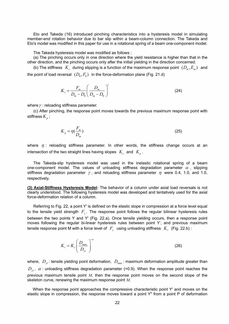
22

Eto and Takeda (16) introduced pinching characteristics into a hysteresis model in simulating

member-end rotation behavior due to bar slip within a beam-column connection. The Takeda and Eto's model was modified in this paper for use in a rotational spring of a beam one-component model.

The Takeda hysteresis model was modified as follows : (a) The pinching occurs only in one direction where the yield resistance is higher than that in the

other direction, and the pinching occurs only after the initial yielding in the direction concerned. (b) The stiffness sK during slipping is a function of the maximum response point ( , )m mD E and

the point of load reversal 0 0( , )D F in the force-deformation plane (Fig. 21.d)

0 0

m ms

m m

F DKD D D D

γ

= − − (24)

whereγ : reloading stiffness parameter.

(c) After pinching, the response point moves towards the previous maximum response point with stiffness pK ;

( )mp

m

FKD

η= (25)

where η : reloading stiffness parameter. In other words, the stiffness change occurs at an intersection of the two straight lines having slopes sK and pK .

The Takeda-slip hysteresis model was used in the inelastic rotational spring of a beam one-component model. The values of unloading stiffness degradation parameter α , slipping stiffness degradation parameter γ , and reloading stiffness parameter η were 0.4, 1.0, and 1.0, respectively.

(3) Axial-Stiffness Hysteresis Model: The behavior of a column under axial load reversals is not clearly understood. The following hysteresis model was developed and tentatively used for the axial force-deformation relation of a column.

Referring to Fig. 22, a point Y' is defined on the elastic slope in compression at a force level equal to the tensile yield strength yF . The response point follows the regular bilinear hysteresis rules between the two points Y and Y' (Fig. 22.a). Once tensile yielding occurs, then a response point moves following the regular bi-linear hysteresis rules between point Y’, and previous maximum tensile response point M with a force level of yF using unloading stiffness rK (Fig. 22.b) :

max

a

r cyt

DK KD

−

=

(26)

where, ytD : tensile yielding point deformation, maxD : maximum deformation amplitude greater than

ytD , α : unloading stiffness degradation parameter (=0.9). When the response point reaches the previous maximum tensile point M, then the response point moves on the second slope of the skeleton curve, renewing the maximum response point M.

When the response point approaches the compressive characteristic point Y' and moves on the elastic slope in compression, the response moves toward a point Y" from a point P of deformation

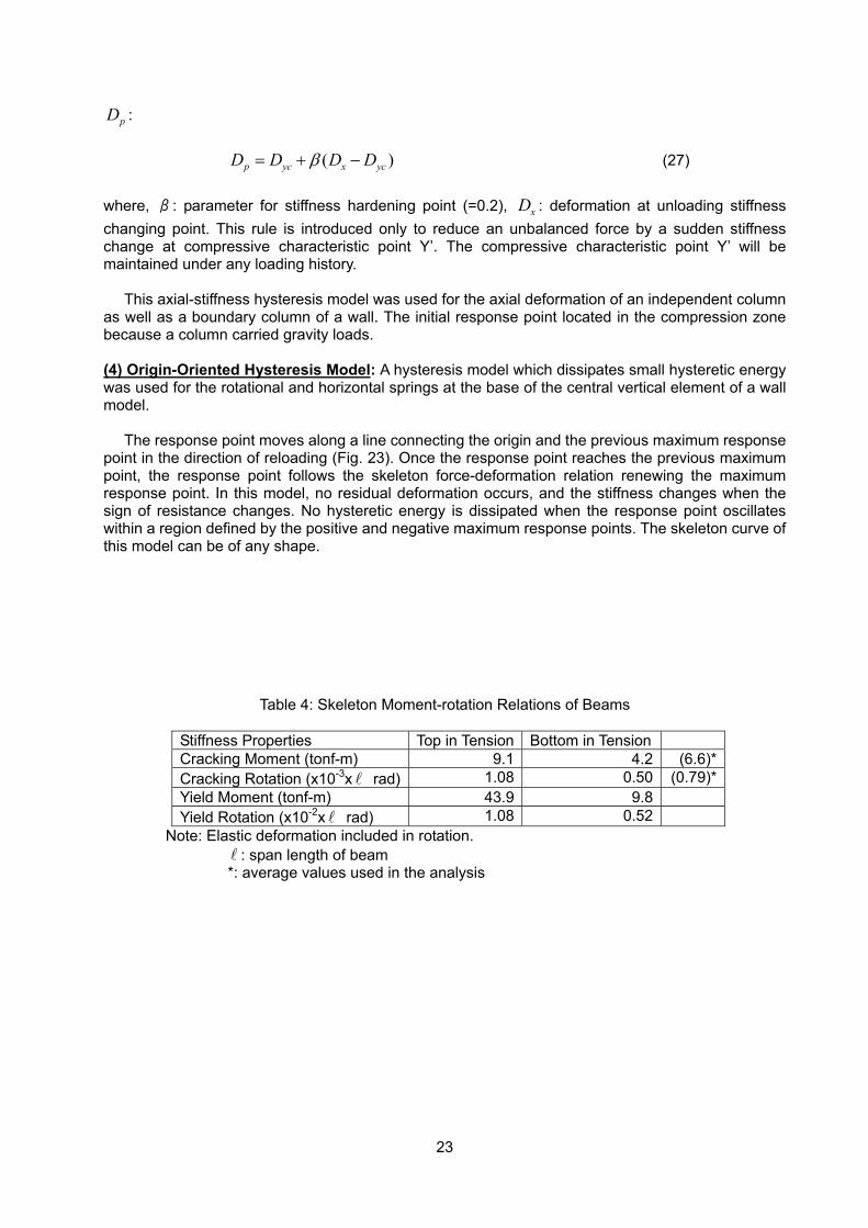
23

pD : ( )p yc x ycD D D Dβ= + − (27)

where, β: parameter for stiffness hardening point (=0.2), xD : deformation at unloading stiffness changing point. This rule is introduced only to reduce an unbalanced force by a sudden stiffness change at compressive characteristic point Y’. The compressive characteristic point Y’ will be maintained under any loading history.

This axial-stiffness hysteresis model was used for the axial deformation of an independent column as well as a boundary column of a wall. The initial response point located in the compression zone because a column carried gravity loads. (4) Origin-Oriented Hysteresis Model: A hysteresis model which dissipates small hysteretic energy was used for the rotational and horizontal springs at the base of the central vertical element of a wall model.

The response point moves along a line connecting the origin and the previous maximum response point in the direction of reloading (Fig. 23). Once the response point reaches the previous maximum point, the response point follows the skeleton force-deformation relation renewing the maximum response point. In this model, no residual deformation occurs, and the stiffness changes when the sign of resistance changes. No hysteretic energy is dissipated when the response point oscillates within a region defined by the positive and negative maximum response points. The skeleton curve of this model can be of any shape.

Table 4: Skeleton Moment-rotation Relations of Beams

Stiffness Properties Top in Tension Bottom in Tension Cracking Moment (tonf-m) 9.1 4.2 (6.6)* Cracking Rotation (x10-3x l rad) 1.08 0.50 (0.79)* Yield Moment (tonf-m) 43.9 9.8 Yield Rotation (x10-2x l rad) 1.08 0.52

Note: Elastic deformation included in rotation. l : span length of beam *: average values used in the analysis

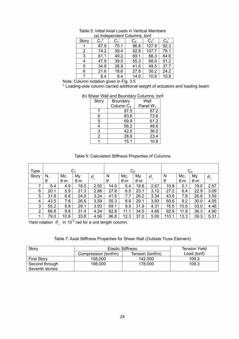
24

Table 5: Initial Axial Loads in Vertical Members (a) Independent Columns, tonf

Story C1* C1’ C2 C3* C3’ 1 87.9 70.1 96.8 127.9 92.3 2 74.2 59.4 82.8 107.7 78.1 3 61.1 49.2 69.1 88.3 64.6 4 47.9 39.0 55.3 68.9 51.2 5 34.8 28.8 41.6 49.5 37.7 6 21.6 18.6 27.8 30.2 24.2 7 8.4 8.4 14.0 10.8 10.8

Note: Column notation given in Fig. 3.5 * Loading-side column carried additional weight of actuators and loading beam

(b) Shear Wall and Boundary Columns, tonf Story Boundary

Column C4

Wall Panel W1

7 97.5 87.26 83.6 73.85 69.9 61.24 56.2 48.63 42.5 36.02 28.8 23.41 15.1 10.8

Table 6: Calculated Stiffness Properties of Columns Type

C1

C2

C3

Story N, tf

Mc, tf-m

My tf-m yθ N

tf Mc, tf-m

My tf-m yθ N

tf Mc, tf-m

My tf-m yθ

7 8.4 4.9 18.5 2.50 14.0 5.4 19.8 2.67 10.8 5.1 19.0 2.576 20.1 5.9 21.3 2.88 27.8 6.5 23.1 3.12 27.2 6.4 22.9 3.095 31.8 6.8 24.0 3.24 41.6 7.7 26.2 3.34 43.6 7.8 26.6 3.594 43.5 7.8 26.6 3.59 55.3 8.8 29.1 3.93 60.6 9.2 30.0 4.053 55.2 8.8 29.1 3.93 69.1 9.9 31.9 4.31 76.5 10.5 33.0 4.462 66.8 9.8 31.4 4.24 82.8 11.1 34.5 4.66 92.9 11.9 36.3 4.901 79.0 10.8 33.8 4.56 96.8 12.3 37.0 5.00 110.1 13.3 39.3 5.31

Yield rotation yθ in 10-3 rad for a unit length column.

Table 7: Axial Stiffness Properties for Shear Wall (Outside Truss Element)

Elastic Stiffness Story Compression (tonf/m) Tension (tonf/m)

Tension Yield Load (tonf)

First Story 158,000 142,000 109.3 Second through Seventh stories

198,000 178,000 109.3

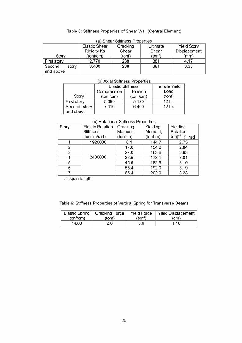
25

Table 8: Stiffness Properties of Shear Wall (Central Element)

(a) Shear Stiffness Properties

Story

Elastic ShearRigidity Ks (tonf/cm)

Cracking Shear (tonf)

Ultimate Shear (tonf)

Yield Story Displacement

(mm) First story 2,770 238 381 4.17 Second story and above

3,400 238 381 3.33

(b) Axial Stiffness Properties

Elastic Stiffness

Story Compression

(tonf/cm) Tension (tonf/cm)

Tensile Yield Load (tonf)

First story 5,690 5,120 121.4 Second story and above

7,110 6,400 121.4

(c) Rotational Stiffness Properties

Story Elastic RotationStiffness (tonf-m/rad)

Cracking Moment (tonf-m)

Yielding Moment, (tonf-m)

Yielding Rotation X10-5 l rad

1 1920000 8.1 144.7 2.75 2 17.6 154.2 2.84 3 27.0 163.6 2.93 4 36.5 173.1 3.01 5 45.9 182.5 3.10 6 55.4 192.0 3.19 7

2400000

65.4 202.0 3.23 l : span length

Table 9: Stiffness Properties of Vertical Spring for Transverse Beams

Elastic Spring (tonf/cm)

Cracking Force(tonf)

Yield Force(tonf)

Yield Displacement (cm)

14.88 2.0 5.6 1.16

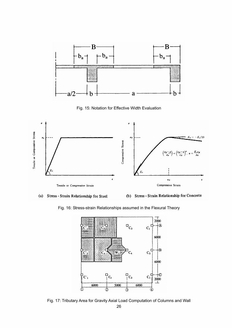
26

Fig. 15: Notation for Effective Width Evaluation

Fig. 16: Stress-strain Relationships assumed in the Flexural Theory

Fig. 17: Tributary Area for Gravity Axial Load Computation of Columns and Wall

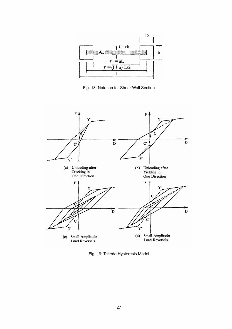
27

Fig. 18: Notation for Shear Wall Section

Fig. 19: Takeda Hysteresis Model

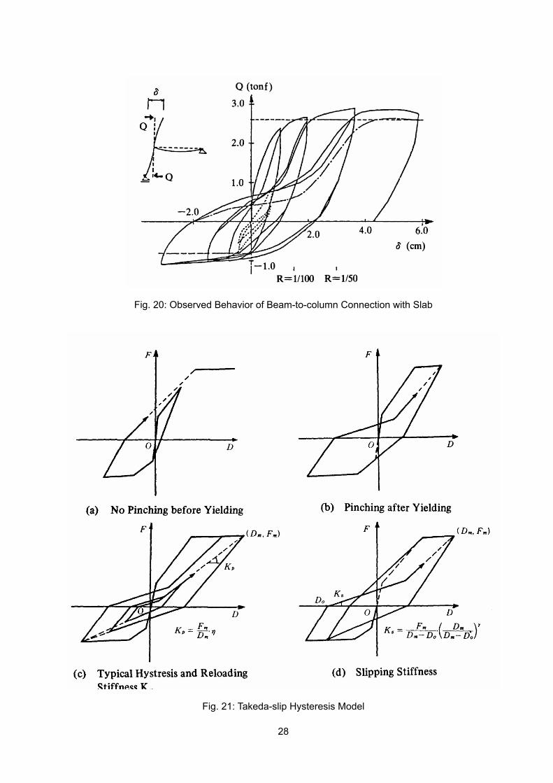
28

Fig. 20: Observed Behavior of Beam-to-column Connection with Slab

Fig. 21: Takeda-slip Hysteresis Model

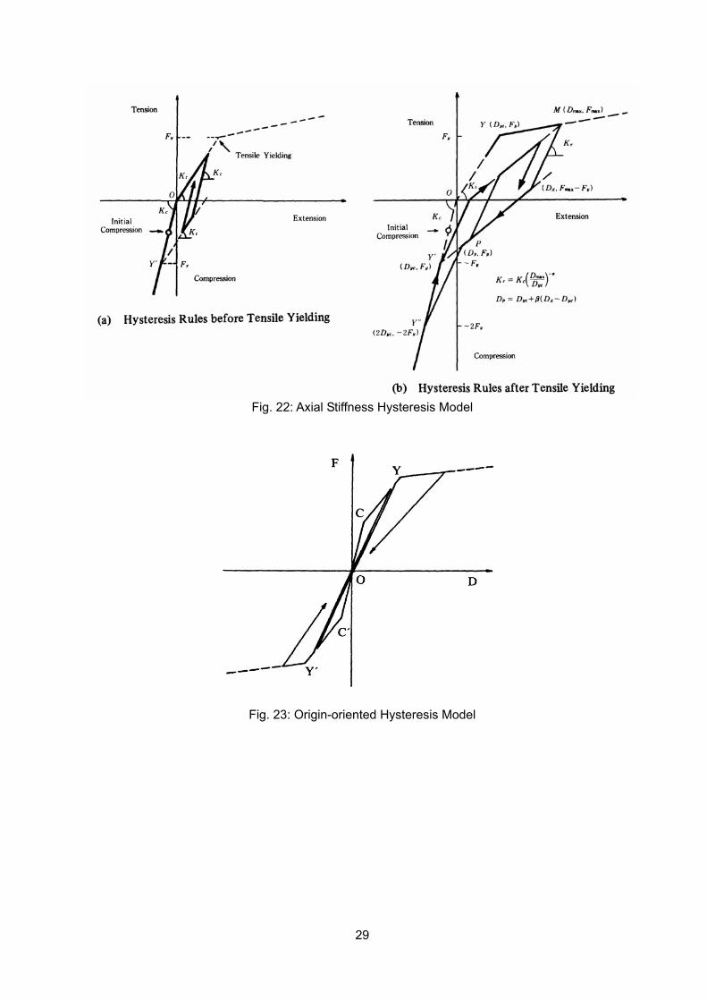
29

Fig. 22: Axial Stiffness Hysteresis Model

Fig. 23: Origin-oriented Hysteresis Model

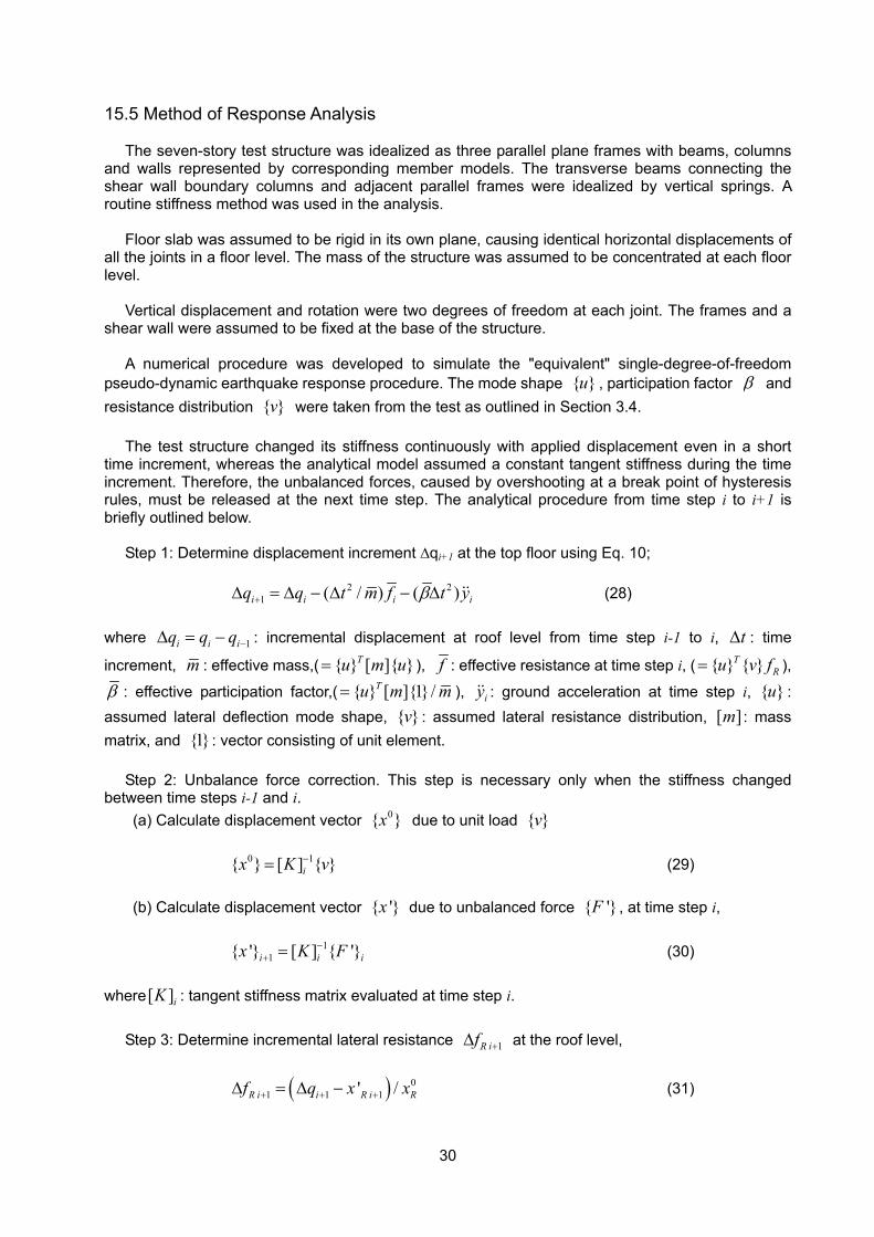
30

15.5 Method of Response Analysis

The seven-story test structure was idealized as three parallel plane frames with beams, columns and walls represented by corresponding member models. The transverse beams connecting the shear wall boundary columns and adjacent parallel frames were idealized by vertical springs. A routine stiffness method was used in the analysis.

Floor slab was assumed to be rigid in its own plane, causing identical horizontal displacements of

all the joints in a floor level. The mass of the structure was assumed to be concentrated at each floor level.

Vertical displacement and rotation were two degrees of freedom at each joint. The frames and a

shear wall were assumed to be fixed at the base of the structure. A numerical procedure was developed to simulate the "equivalent" single-degree-of-freedom

pseudo-dynamic earthquake response procedure. The mode shape { }u , participation factor β and resistance distribution { }v were taken from the test as outlined in Section 3.4.

The test structure changed its stiffness continuously with applied displacement even in a short

time increment, whereas the analytical model assumed a constant tangent stiffness during the time increment. Therefore, the unbalanced forces, caused by overshooting at a break point of hysteresis rules, must be released at the next time step. The analytical procedure from time step i to i+1 is briefly outlined below.

Step 1: Determine displacement increment ∆qi+1 at the top floor using Eq. 10; 2 2

1 ( / ) ( )i i i iq q t m f t yβ+∆ = ∆ − ∆ − ∆ && (28)

where 1i i iq q q −∆ = − : incremental displacement at roof level from time step i-1 to i, t∆ : time

increment, m : effective mass,( { } [ ]{ }Tu m u= ), f : effective resistance at time step i, ( { } { }TRu v f= ),

β : effective participation factor,( { } [ ]{1}/Tu m m= ), iy&& : ground acceleration at time step i, { }u : assumed lateral deflection mode shape, { }v : assumed lateral resistance distribution, [ ]m : mass matrix, and {1} : vector consisting of unit element.

Step 2: Unbalance force correction. This step is necessary only when the stiffness changed between time steps i-1 and i.

(a) Calculate displacement vector 0{ }x due to unit load { }v 0 1{ } [ ] { }ix K v−= (29) (b) Calculate displacement vector { '}x due to unbalanced force { '}F , at time step i, 1

1{ '} [ ] { '}i i ix K F−+ = (30)

where[ ]iK : tangent stiffness matrix evaluated at time step i.

Step 3: Determine incremental lateral resistance 1R if +∆ at the roof level, ( ) 0

1 1 1' /R i i R i Rf q x x+ + +∆ = ∆ − (31)

31

in which 'Rx and 0Rx are the values of vectors { '}x and 0{ }x evaluated at the roof level.

Step 4: Calculate displacement increment { }ix∆ due to incremental load and unbalanced forces

{ '}iF , 0

1 1{ } { } { '}i R i ix x f x+ +∆ = ∆ + (32) Step 5: Calculate incremental member forces from incremental joint displacement and

tangent member stiffness. Check if member stiffness changed during time step i and i+1. Steps 1 through 5 were repeated for each time step. Computed response was temporarily stored

on computer files, and plots of response waveforms and force-deformation curves were made if necessary.

32

15.6 Results of Analysis The analytical models and procedure described above was applied to the full-scale seven-story

test structure. Equivalent single-degree-of-freedom pseudo-dynamic tests PSD-2 through PSD-4 were simulated continuously so that the structural damage in the preceding test runs could be reflected in the analysis of the following test runs. In other words, the analytical model was given the calculated residual displacement and structural damage from the immediately preceding test run. Initial velocity of the analytical model was set to be null at the beginning of each test run. The actual test was conducted in the same manner.

Pseudo-dynamic test PSD-1 was not analyzed herein because the test run was carried out to

examine the reliability of the testing technique and procedure. The maximum roof-level displacement was as small as 1/8600 of the total structural height. The structure was observed to remain in the elastic range during the test run. Therefore, the test run was not included for study here.

The analytical response of test PSD-3 was studied in detail to examine the reliability of the

analytical method. The structure was subjected to a displacement beyond the formation of collapse mechanism during the test run. The roof-level displacement was observed to reach 1/91 the total story height, a displacement which may be expected from this type of a structure during a "strong" earthquake motion. This test included a wide range of response prior to and after the yielding of various members and the shear wall. The structure did not have non-structural elements. These were major reasons to choose this particular test run for careful inspection. Studied are the analytical results of (a) response waveforms at the roof level displacement and base shear, (b) hysteresis relation between base shear and roof-level displacement, (c) base shear-local deformation relations, and (d) force and deformation distribution at maximum computed response.

The calculated response waveforms and the roof-level displacement vs. base shear relations are

briefly compared with the observed for tests PSD-2 and PSD4.

Response Waveforms (Test PSD-3): The artificial earthquake accelerogram based on EW component of the Taft record (1952) was used in test PSD-3. The higher frequency components were removed from the original record so that the first mode should govern the response of the test structure. The maximum ground acceleration was 320 Gal (cm/sec2).

No damping was assumed in the test structure in the pseudo-dynamic response computation

during the test. Observed and calculated response waveforms are compared for the roof-level displacement and base shear as shown in Fig. 24. The input base motion is shown in the same figure. Note that the base motion oscillates in relatively low frequency compared with the original earthquake record.

Response waveforms observed in test PSD-3 are shown in broken lines. Analytical responses are

in good agreement with the observed response over the entire duration of earthquake excitation. Maximum displacement at roof-level was 238 mm from the test attained at 4.48 sec, while the

calculated maximum amplitude was slightly larger (= 248 mm) than the observed. Both maxima occurred at the same time step. The period of oscillation elongated significantly after this time step in the test and analysis.

At 10.16 second, the ground motion input was terminated in the test, and pseudo-dynamic

free-vibration test was started with existing residual displacement and no velocity. In the free vibration range, the period of the analytical model appeared slightly longer than that of the test structure.

Maximum base shear of 414 tonf was attained at 4.48 sec in the test. The computed value was

425 tonf, slightly higher than the observed. Maximum base shear amplitude of an analytical model can easily be controlled by choosing yield resistance level and post-yielding stiffness of constituent members, especially of beam members in this analysis.

33

Parametric studies by varying beam yield resistance and post-yielding stiffness indicated that the combination of the values described in Chapter 5 was most suited to the test structure; i.e., the beam yield resistance to be computed with the contribution of slab reinforcement within an effective width of 430 cm and post-yielding stiffness to be 3 % of the initial elastic stiffness.

SDF Hysteresis Relation (Test PSD-3): Roof-level displacement and base shear were the corresponding force and displacement in the "equivalent" single-degree-of-freedom pseudo-dynamic test, and their relation may be called "SDF hysteresis" as shown in Fig. 25.

As can be expected from a good correlation of observed and computed response waveforms, the

observed and computed hysteresis relations as an equivalent single-degree-of-freedom system are in fair agreement, especially at the peaks of hysteresis loops. General shapes of the two curves are slightly different; the stiffness of the test structure changed gradually during unloading, whereas the stiffness of the analytical model changed when the sign of resistance changed. The latter stiffness change was associated with that of member hysteresis models such as Takeda, Takeda-slip, and Origin-oriented hysteresis models. The analytical model showed some pinching behavior, which was also appreciable in the observed hysteresis relation. The pinching behavior of an analytical model was caused by Takeda-slip hysteresis model used with beam one-component models and axial-stiffness hysteresis model used with vertical line elements in the shear wall.

Local Deformations (Test PSD-3): During the pseudo-dynamic tests, local deformations of members were measured at various locations of the test structure; (a) flexural rotation at beam ends, (b) flexural rotation at column base, (c) elongation of boundary columns of the wall, and (d) shear deformation of the wall panel. Computed local deformations of typical members were compared with the observed deformations so as to examine the reliability of the analysis method.

(1) Beam End Rotation: Rotations at beam ends were determined from the axial elongation and compression measurements by two displacement gauges, one placed above the slab face and the other placed below the beam, parallel to the beam member axis (Fig. 26.c). The gauge length was one half the effective beam depth from the column face.

The observed base shear-beam end rotation relation of a sixth floor beam at the wall connection is

shown in Fig. 26.a. The calculated relation is shown in Fig. 26.b. The calculated and the observed relations do not necessarily agree because the beam end rotation was measured for a given gauge length, whereas the rotation was calculated for an entire beam under imaginary anti-symmetric loading condition. In other words, the calculated deformation corresponds to the deformation over one-half span length of the beam. Therefore, the measured deformations were generally smaller, and approximately 60 to 70% of the calculated amplitudes. General shapes of the base shear-beam end rotation relation curves of the two were similar.

The beam was subjected to larger deformation in the negative loading direction when the

connecting tension-side boundary column moved upward. The upward displacement of a boundary column joint (node) was significantly larger than the downward displacement because the bending deformation of a wall was mainly attributable to the elongation of a tension-side boundary column. Both observed and calculated beam-end response show this behavior.

Negative maximum deformations were larger than the positive deformation, although positive and

negative amplitudes of overall structural displacement were comparable. Negative deformation amplitudes at the two ends of the beam were comparable, whereas the positive deformation at the wall end was approximately 1.3 times larger than that of the behavior observed at the further end (left end); the behavior was observed both in the measured and calculated beam-end rotations. At the exterior column-beam joint, beam negative moment capacity was large due to the participation of slab reinforcement. Hence, the exterior column was subjected to higher bending moment under the positive loading (load applied from right to left), and experienced a larger rotation at column ends. Therefore, nodal rotation at the exterior beam-column joint under the positive loading was smaller, resulting in a smaller beam-end rotation at the exterior column end.

34

Figure 27 shows the beam-end rotations at a sixth floor beam in Frame A. The observed

beam-end rotation amplitudes were smaller than the calculated amplitudes.

(2) Column Axial Deformation: A large vertical displacement was observed at the top (roof level) of the tension-side boundary column of the wall during the test. Large axial elongations were measured in the tensile region of the wall, especially at lower stories. Compressive axial deformations in the corresponding region were small under opposite direction loading. Larger deformation was observed in a transverse beam connected at the tensile edge (boundary column) of the wall. The boundary columns were measured to elongate as much as 44 mm in the first story as shown in Fig. 28.a, whereas the maximum compressive deformation reached only 5 mm.

Computed axial deformations of the boundary column, as expressed as the deformation of outer

truss elements, are shown in Fig. 28.b. General deformation amplitudes and hysteresis shapes of the analytical model agree reasonably well with those of the test structure. The computed axial deformation was larger.

Response at Maximum Displacement (Test PSD-3): It is important from design point of view to estimate possible force amplitudes and deformation ductility factors at various critical sections of the test structure at maximum deformation. However, member forces could not be measured in the test. The frame analysis method may be applied to estimate these quantities. The maximum deformation of the test structure was observed as well as calculated to occur at 4.48 see of the earthquake time.

(1) Member Forces: Member forces in wall-frame B calculated at maximum structural deformation by the analytical model are shown in Fig. 29. The wall carried smaller shear forces in the first story than in the second story.

Vertical forces transferred by transverse beams to the wall boundary columns are also shown in

the figure. Yield force level was reached by the transverse beam connected to the boundary column in tension.

(2) Member Ductility: Ductility factors are defined in the analysis as a ratio of maximum deformation amplitude to the calculated yield amplitude. Figure 30 shows the distribution of ductility factors at the maximum structural deformation for frames A and C and frame B.

In open frames A and C (Fig. 30.a), almost all beam ends yielded at the maximum displacement

except those at the roof level. Under this deformed configuration, the top chord was in tension at the left end of a beam, and the bottom chord was in tension at the right end. Ductility factors, ratios of beam end rotations to the yield rotation, ranged from 0.8 to 1.5 at the left end of the beams, and from 2.3 to 4.7 at the right end. The rotation amplitudes at the left and right ends of the beams are comparable. The difference in ductility factors at the two ends of a beam was caused by the difference in the yield rotations at the two ends (see Table 4); the yield: rotation amplitude under negative moment (top chord in tension) is approximately twice as much as that under positive moment (bottom chord in tension).

Ductility factors at the same end (left or right) of the beams varied with the level of the beam; the

ductility factor decreased with the beam level. A beam end rotation appeared to be inversely related to the column end rotation of the joint. Ductility factors of beam ends were smaller at the upper floor levels where the columns yielded, and they were larger at the right exterior joints where the column rotations were smaller.

In wall-frame B (Fig. 30.b), all beams yielded. Under the deformed configuration, the top chord

was in tension at the left end of a beam, and the bottom chord in tension at right end. The distribution of beam end ductility factors was relatively uniform along the height; 1.4 to 1.7 at left exterior beam ends, 4.1 to 4.7 at beam ends immediately left of the wall, 3.2 to 3.4 at beam ends immediately right of the wall, and 6.5 to 7.9 at right exterior beam ends. The beam end rotation was generally larger in the right exterior span than that at the corresponding end in the left exterior beams, which was

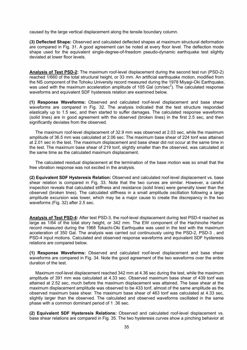
35

caused by the large vertical displacement along the tensile boundary column.

(3) Deflected Shape: Observed and calculated deflected shapes at maximum structural deformation are compared in Fig. 31. A good agreement can be noted at every floor level. The deflection mode shape used for the equivalent single-degree-of-freedom pseudo-dynamic earthquake test slightly deviated at lower floor levels.

Analysis of Test PSD-2: The maximum roof-level displacement during the second test run (PSD-2) reached 1/660 of the total structural height, or 33 mm. An artificial earthquake motion, modified from the NS component of the Tohoku University record measured during the 1978 Miyagi-Oki Earthquake, was used with the maximum acceleration amplitude of 105 Gal (cm/sec2). The calculated response waveforms and equivalent SDF hysteresis relation are examined below.

(1) Response Waveforms: Observed and calculated roof-level displacement and base shear waveforms are compared in Fig. 32. The analysis indicated that the test structure responded elastically up to 1.5 sec, and then started to suffer damages. The calculated response waveforms (solid lines) are in good agreement with the observed (broken lines) in the first 2.5 sec, and then significantly deviates from the observed.

The maximum roof-level displacement of 32.9 mm was observed at 2.03 sec, while the maximum

amplitude of 36.5 mm was calculated at 2.06 sec. The maximum base shear of 224 tonf was attained at 2.01 sec in the test. The maximum displacement and base shear did not occur at the same time in the test. The maximum base shear of 219 tonf, slightly smaller than the observed, was calculated at the same time as the calculated maximum displacement.

The calculated residual displacement at the termination of the base motion was so small that the

free vibration response was not excited in the analysis.

(2) Equivalent SDF Hysteresis Relation: Observed and calculated roof-level displacement vs. base shear relation is compared in Fig. 33. Note that the two curves are similar. However, a careful inspection reveals that calculated stiffness and resistance (solid lines) were generally lower than the observed (broken lines). The calculated stiffness in a small amplitude oscillation following a large amplitude excursion was lower, which may be a major cause to create the discrepancy in the two waveforms (Fig. 32) after 2.5 sec.

Analysis of Test PSD-4: After test PSD-3, the roof-level displacement during test PSD-4 reached as large as 1/64 of the total story height, or 342 mm. The EW component of the Hachinohe Harbor record measured during the 1968 Tokachi-Oki Earthquake was used in the test with the maximum acceleration of 350 Gal. The analysis was carried out continuously using the PSD-2, PSD-3 , and PSD-4 input motions. Calculated and observed response waveforms and equivalent SDF hysteresis relations are compared below.

(1) Response Waveforms: Observed and calculated roof-level displacement and base shear waveforms are compared in Fig. 34. Note the good agreement of the two waveforms over the entire duration of the test.

Maximum roof-level displacement reached 342 mm at 4.36 sec during the test, while the maximum

amplitude of 391 mm was calculated at 4.33 sec. Observed maximum base shear of 439 tonf was attained at 2.52 sec, much before the maximum displacement was attained. The base shear at the maximum displacement amplitude was observed to be 433 tonf, almost of the same amplitude as the observed maximum base shear. The maximum base shear of 463 tonf was calculated at 4.33 sec, slightly larger than the observed. The calculated and observed waveforms oscillated in the same phase with a common dominant period of 1 .36 sec.

(2) Equivalent SDF Hysteresis Relations: Observed and calculated roof-level displacement vs. base shear relations are compared in Fig. 35. The two hysteresis curves show a pinching behavior at

36

low stress levels. As expected from the good agreement in the response waveforms, the two hysteresis curves agreed well. The observed base shear in the positive direction was slightly lower than that in the negative direction. Such degradation in resistance was not reproduced by the analytical model.

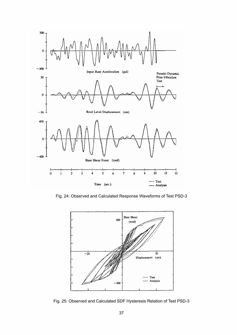
37

Fig. 24: Observed and Calculated Response Waveforms of Test PSD-3

Fig. 25: Observed and Calculated SDF Hysteresis Relation of Test PSD-3

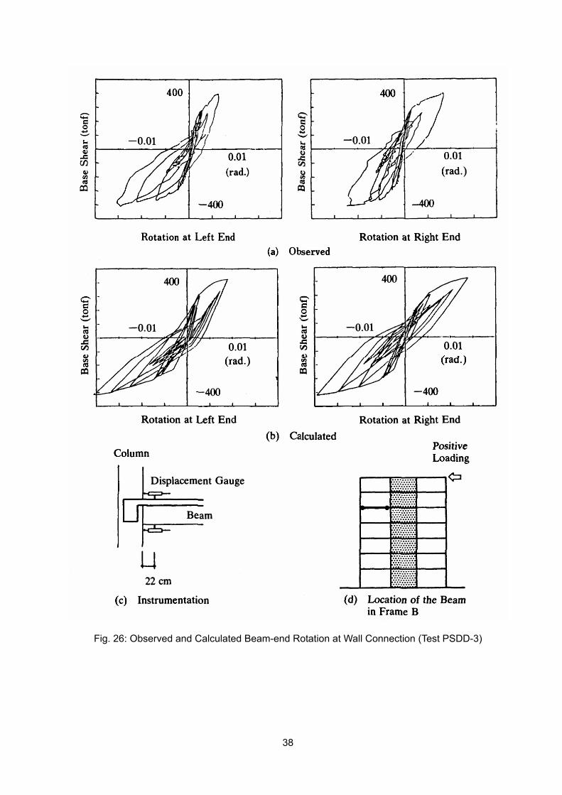
38

Fig. 26: Observed and Calculated Beam-end Rotation at Wall Connection (Test PSDD-3)

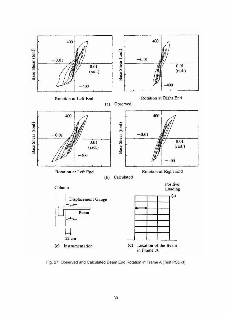
39

Fig. 27: Observed and Calculated Beam End Rotation in Frame A (Test PSD-3)

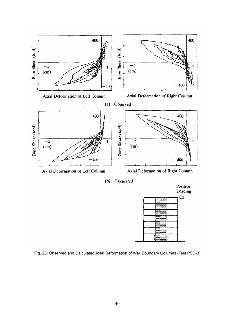
40

Fig. 28: Observed and Calculated Axial Deformation of Wall Boundary Columns (Test PSD-3)

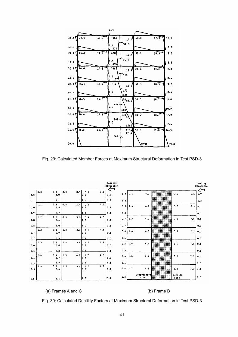
41

Fig. 29: Calculated Member Forces at Maximum Structural Deformation in Test PSD-3

(a) Frames A and C (b) Frame B

Fig. 30: Calculated Ductility Factors at Maximum Structural Deformation in Test PSD-3

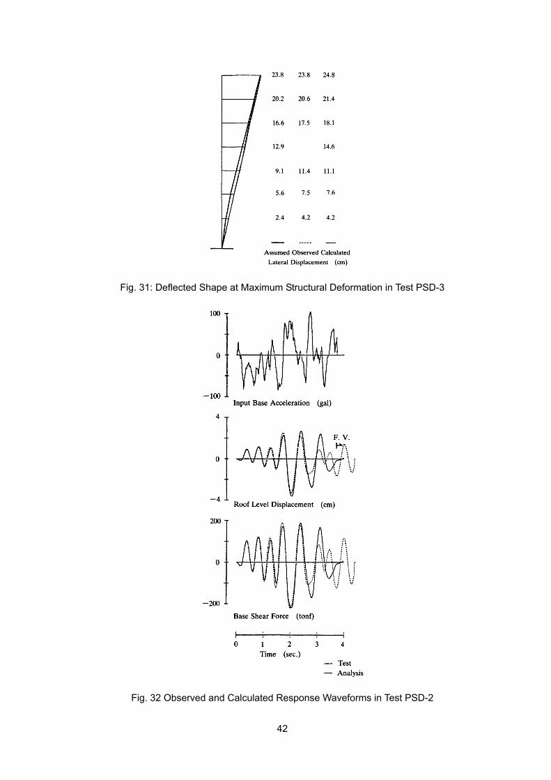
42

Fig. 31: Deflected Shape at Maximum Structural Deformation in Test PSD-3

Fig. 32 Observed and Calculated Response Waveforms in Test PSD-2

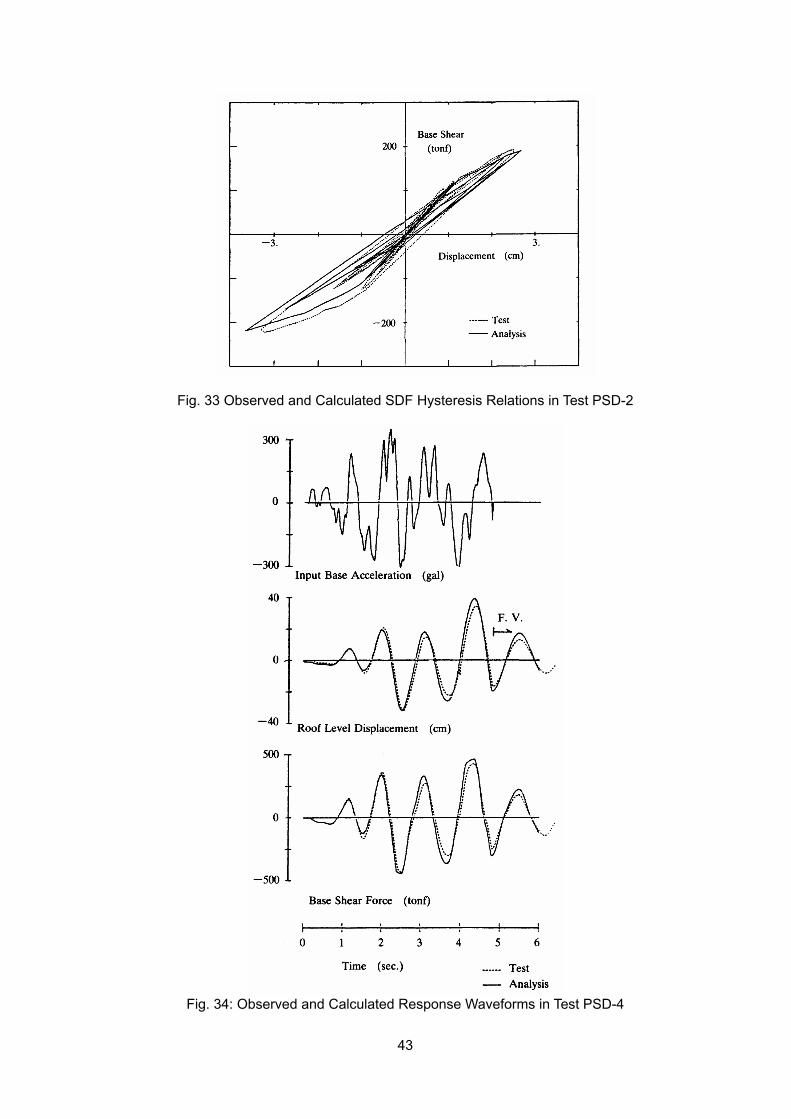
43

Fig. 33 Observed and Calculated SDF Hysteresis Relations in Test PSD-2

Fig. 34: Observed and Calculated Response Waveforms in Test PSD-4

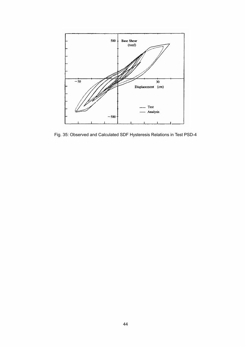
44

Fig. 35: Observed and Calculated SDF Hysteresis Relations in Test PSD-4

45

15.7 Concluding Remarks A full-scale seven-story reinforced concrete structure was tested using "equivalent"

single-degree-of-freedom pseudo-dynamic earthquake response test procedure at Building Research Institute, Tsukuba, as a part of U.S.-Japan Cooperative Research Program Utilizing Large Scale Testing Facilities.

A nonlinear dynamic analysis method was used to simulate the observed behavior. The method

utilized three different member models for (a) beams and columns, (b) shear walls, and (c) transverse beams, and four hysteresis models for elements of member models: (a) Takeda hysteresis model, (b) Takeda-slip hysteresis model, (c) Axial-stiffness hysteresis model, and (d) Origin-oriented hysteresis model.

A procedure was outlined as to the method to determine stiffness properties used for the analysis

on the basis of material properties and structural geometry. The response of the test structure was computed by a numerical procedure specially developed to

simulate the "equivalent" single-degree-of-freedom pseudo-dynamic earthquake response test procedure.

A good correlation was reported between the observed and calculated response when the

structure responded well in an inelastic range. However, it was felt more difficult to attain a good correlation when the structural response reached barely yielding.

The method of nonlinear dynamic analysis of reinforced concrete buildings can be made

significantly reliable not only to outline the overall structural behavior, but also to describe the local behavior.

References:

1) Wight, J.K. and S. Nakata, “Construction of the Full-scale Seven-story Reinforced Concrete Test Structure,” Report Presented during The Second Joint Technical Coordinating Committee, U.S.-Japan Cooperative Earthquake Research Program Utilizing Large-Scale Testing Facilities, Tsukuba, Japan, 1982.

2) Okamoto, S., S. Nakata, Y. Kitagawa, M. Yoshimura and T. Kaminosono, “A Progress Report on the

Full-scale Seismic Experiment of a Seven-story Reinforced Concrete Building - Part of the U.S.-Japan Cooperative Program,” BRI Research Paper No. 94, Building Research Institute, Ministry of Construction, 1982.

3) Otani, S., “Nonlinear Dynamic Analysis of Reinforced Concrete Building Structures,” Canadian

Journal of Civil Engineering, Vol. 7, No. 2, 1980, pp. 333 - 344. 4) Umemura, H. and H. Takizawa, “A State-Of-the-Art Report On the Dynamic Response of

Reinforced Concrete Buildings,” Structural Engineering Documents 2, IABSE, 1981. 5) Giberson, M. F., “The Response of Nonlinear Multi-Story Structures Subjected to Earthquake

Excitation,” Earthquake Engineering Research Laboratory, EERL Report, California Institute of Technology, Pasadena, California, 1967.

6) Clough, R. W., K. L. Wilson, “Inelastic Earthquake Response of Tall Building,” Proceedings, Third

World Conference on Earthquake Engineering, New Zealand, Vol. II Section II, 1965, pp. 68 - 89. 7) Otani, S. and M. A. Sozen, “Behavior of Multistory Reinforced Concrete Frames during

Earthquake,” Structural Research Series No. 392, Department of Civil Engineering, University of Illinois, Urbana, 1972.

46

8) Takizawa, H., “Strong Motion Response Analysis of Reinforced Concrete Buildings (in Japanese),” Concrete Journal, Japan National Council on Concrete, Vol. 11, No. 2, 1973, pp. 10 - 21.

9) Omote, Y. and T. Takeda, “Nonlinear Earthquake Response Study on the Reinforced Concrete

Chimney - Part 1 Model Tests and Analysis (in Japanese),” Transactions, Architectural Institute of Japan, No. 215, 1974, pp. 21-32.

10) Takayanagi, T. and W. C. Schnobrich, “Computed Behavior of Reinforced Concrete Coupled

Shear Walls,” Structural Research Series No. 434, University of Illinois, Urbana, 1976. 11) Hiraishi, H., M. Yoshimura, H. Isoishi and S. Nakata, “Planer Tests on Reinforced Concrete Shear

Wall Assemblies - U.S.-Japan Cooperative Research Program -, Report submitted at Joint Technical Coordinating Committee, U.S.-Japan Cooperative Research Program, Building Research Institute of Japan, 1981.

12) Architectural Institute of Japan: AIJ Standard for Structural Calculation of Reinforced Concrete

Structures (Revised in 1982), 1950. 13) Hirosawa, M., “Past Experimental Results on Reinforced Concrete Shear Walls and Analysis on

them (in Japanese),” Kenchiku Kenkyu Shiryo No. 6, Building Research Institute, Ministry of Construction, 1975.

14) Takeda, T., M. A. Sozen and N. N. Nielsen, “Reinforced Concrete Response to Simulated

Earthquakes,” ASCE, Journal of the Structural Division, Vol. 96, No. ST12, 1970, pp. 2557 - 2573. 15) Nakata, S., S. Otani; T. Kabeyasawa, Y. Kai and S. Kimura, “Tests of Reinforced Concrete

Beam-Column Assemblages, - U.S.-Japan Cooperative Research Program -,” Report submitted to Joint Technical Coordinating Committee, U.S.-Japan Cooperative Research Program, Building Research Institute and University of Tokyo, 1980.

16) Eto. H. and T. Takeda, “Elasto Plastic Earthquake Response Analysis of Reinforced Concrete

Frame Structure (in Japanese),” Proceedings, Architectural Institute of Japan Annual Meeting, 1977, pp. 1877 - l878.

17) Fujii, S, H. Aoyama and H. Umemura, “Moment-Curvature Relations of Reinforced Concrete

Sections Obtained from Material Characteristics (in Japanese),” Proceedings, Architectural Institute of Japan Annual Meeting, 1973, pp. 1261 - 1262.

18) Kaminosono. T., S. Okamoto, Y. Kitagawa, S. Nakata, M. Yoshimura, S. Kurose and H. Tsubosaki,

“The Full-Scale Seismic Experiment of a Seven-story Reinforced Concrete Building, - Part 1, 2 - (in Japanese” Proceedings, Sixth Japan Earthquake Engineering Symposium, 1982, pp. 865-880.

19) Sugano, S., “Experimental Study on Restoring Force Characteristics of Reinforced Concrete

Members (in Japanese),” Doctor of Engineering Thesis, Department of Architecture, University of Tokyo, 1970.