Oti i tiOptimization and PfP erformance Analysis of High ... · Not backward compatible with previous UMTS. HSPA architecture (UMTS, HSDPA, HSUPA) UE: User Equipment USIM: ... q i

O ti i ti d P fOptimization and Performance Analysis of High Speed Mobile A N t kAccess Networks

Thushara Weerawardane

ComNets, University of Bremen, Germany

03.09.2010

[email protected]‐bremen.de

Overview

Overview of high speed broadband wireless networksKey technologies and architecture

M i hiMain achievementsOverview of the completed tasks during the thesis work

HSPA transport flow control and congestion controlp gTheoretical approach

Analytical modeling

Performance analysis and results comparisonPerformance analysis and results comparison

Conclusion and outlook

[email protected]‐bremen.de 2

High speed broadband wireless networks

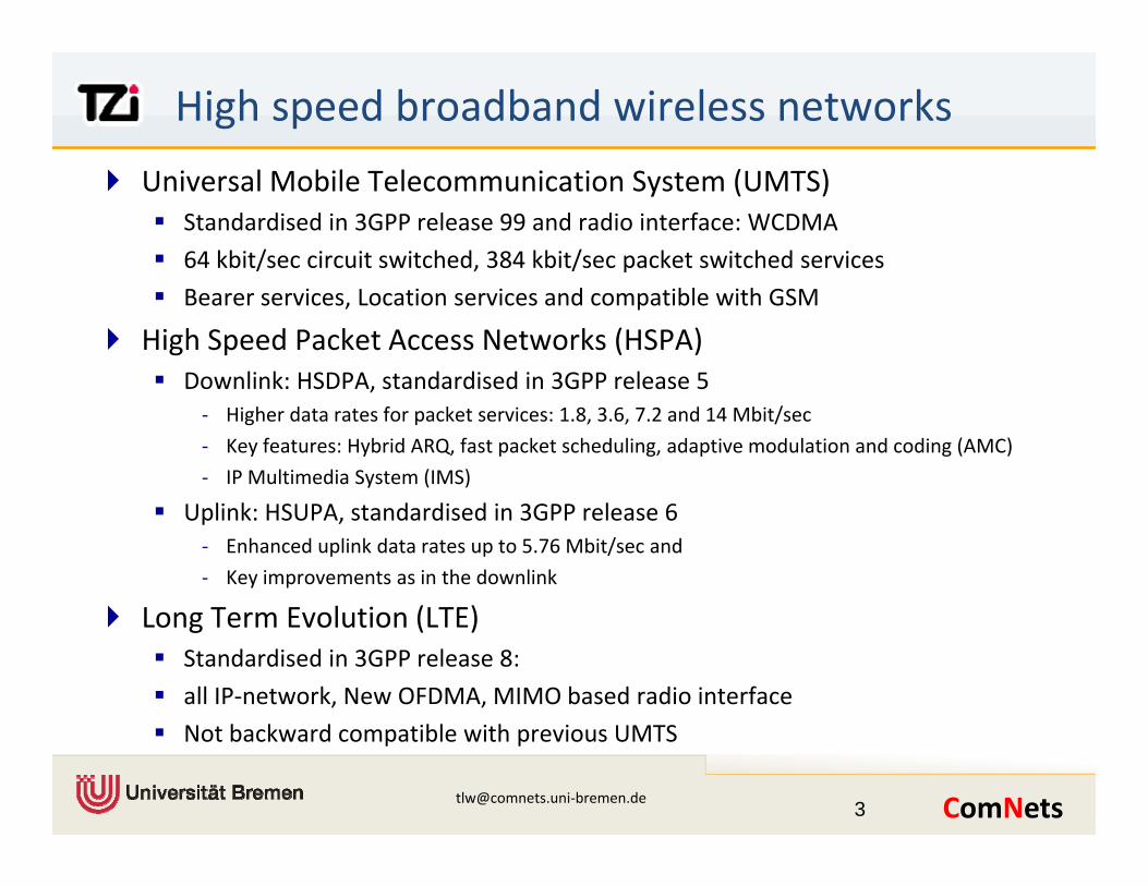
Universal Mobile Telecommunication System (UMTS) Standardised in 3GPP release 99 and radio interface: WCDMA

64 kbit/sec circuit switched, 384 kbit/sec packet switched services

Bearer services, Location services and compatible with GSM

High Speed Packet Access Networks (HSPA)Downlink: HSDPA, standardised in 3GPP release 5Downlink: HSDPA, standardised in 3GPP release 5‐ Higher data rates for packet services: 1.8, 3.6, 7.2 and 14 Mbit/sec

‐ Key features: Hybrid ARQ, fast packet scheduling, adaptive modulation and coding (AMC)

‐ IP Multimedia System (IMS)

Uplink: HSUPA, standardised in 3GPP release 6‐ Enhanced uplink data rates up to 5.76 Mbit/sec and

‐ Key improvements as in the downlink

L T E l ti (LTE)Long Term Evolution (LTE)Standardised in 3GPP release 8:

all IP‐network, New OFDMA, MIMO based radio interface


Not backward compatible with previous UMTS

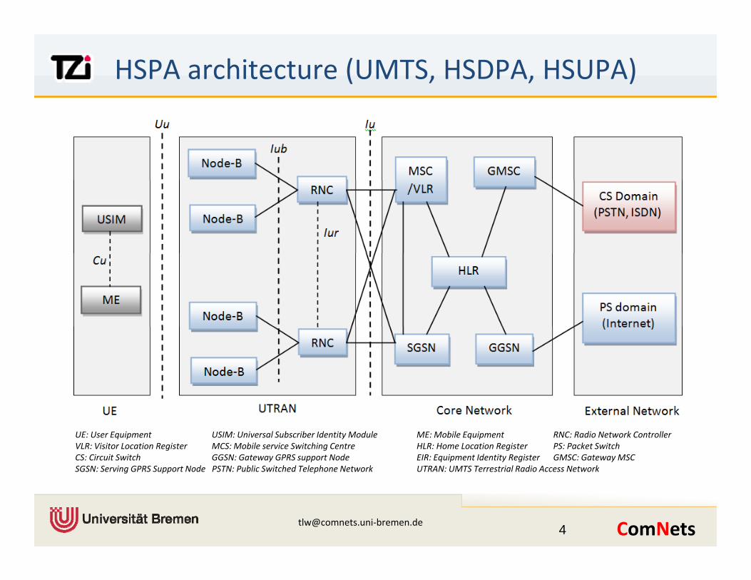
HSPA architecture (UMTS, HSDPA, HSUPA)

UE: User Equipment USIM: Universal Subscriber Identity Module ME: Mobile Equipment RNC: Radio Network ControllerVLR: Visitor Location Register MCS: Mobile service Switching Centre HLR: Home Location Register PS: Packet SwitchCS: Circuit Switch GGSN: Gateway GPRS support Node EIR: Equipment Identity Register GMSC: Gateway MSC SGSN: Serving GPRS Support Node PSTN: Public Switched Telephone Network UTRAN: UMTS Terrestrial Radio Access Network


g pp p

Key achievements

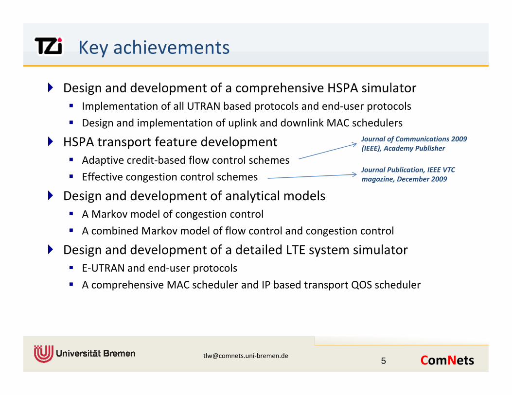
Design and development of a comprehensive HSPA simulatorImplementation of all UTRAN based protocols and end‐user protocols

Design and implementation of uplink and downlink MAC schedulersDesign and implementation of uplink and downlink MAC schedulers

HSPA transport feature developmentAdaptive credit‐based flow control schemes

ff l h

Journal of Communications 2009 (IEEE), Academy Publisher

Journal Publication, IEEE VTC Effective congestion control schemes

Design and development of analytical modelsA Markov model of congestion control

,magazine, December 2009

A combined Markov model of flow control and congestion control

Design and development of a detailed LTE system simulatorE‐UTRAN and end‐user protocolsp

A comprehensive MAC scheduler and IP based transport QOS scheduler


Key achievements

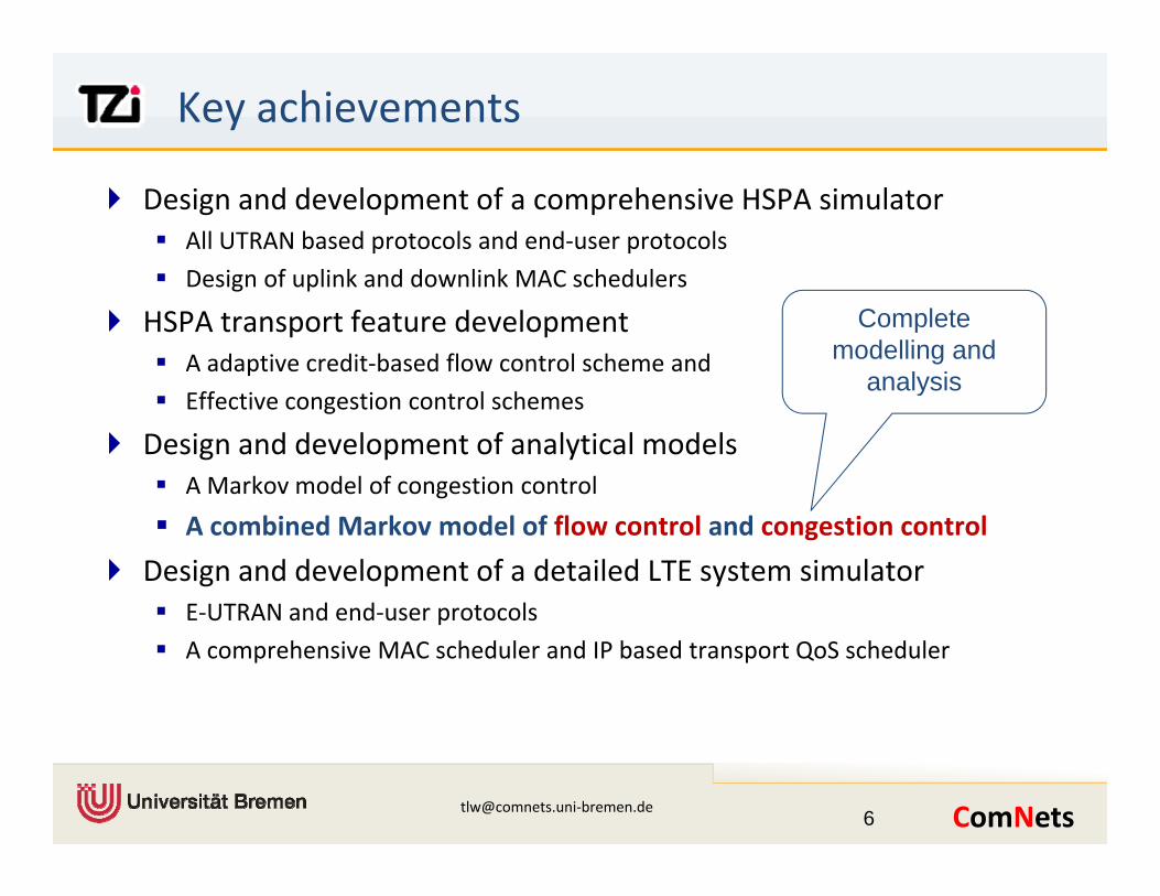
Design and development of a comprehensive HSPA simulatorAll UTRAN based protocols and end‐user protocols

Design of uplink and downlink MAC schedulersDesign of uplink and downlink MAC schedulers

HSPA transport feature developmentA adaptive credit‐based flow control scheme and

ff l h

Complete modelling and

analysis Effective congestion control schemes

Design and development of analytical modelsA Markov model of congestion control

y

A combined Markov model of flow control and congestion control

Design and development of a detailed LTE system simulatorE‐UTRAN and end‐user protocolsE UTRAN and end user protocols

A comprehensive MAC scheduler and IP based transport QoS scheduler


HSDPA FC and CC overview

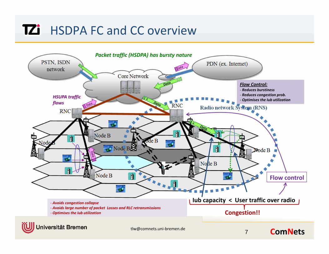
Packet traffic (HSDPA) has bursty nature

Flow Control:‐ Reduces burstiness ‐ Reduces congestion prob.‐ Optimises the Iub utilization

HSUPA traffic flows

Flow control

User traffic over radioIub capacity <‐ Avoids congestion collapseA oids large n mber of packet Losses and RLC retransmissions


Congestion!!‐ Avoids large number of packet Losses and RLC retransmissions‐ Optimises the Iub utilization

HSDPA flow control and congestion control

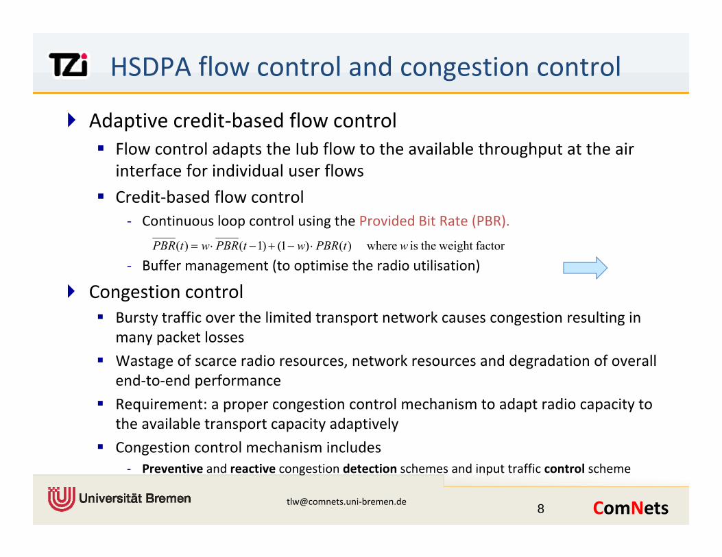
Adaptive credit‐based flow controlFlow control adapts the Iub flow to the available throughput at the air interface for individual user flowsinterface for individual user flows

Credit‐based flow control ‐ Continuous loop control using the Provided Bit Rate (PBR).

f ti htthih)()1()1()( tPBRtPBRtPBR +

‐ Buffer management (to optimise the radio utilisation)

Congestion controlB t t ffi th li it d t t t k ti lti i

factor weight theiswhere)()1()1()( wtPBRwtPBRwtPBR ⋅−+−⋅=

Bursty traffic over the limited transport network causes congestion resulting in many packet losses

Wastage of scarce radio resources, network resources and degradation of overall end‐to‐end performanceend to end performance

Requirement: a proper congestion control mechanism to adapt radio capacity to the available transport capacity adaptively

Congestion control mechanism includes


g‐ Preventive and reactive congestion detection schemes and input traffic control scheme

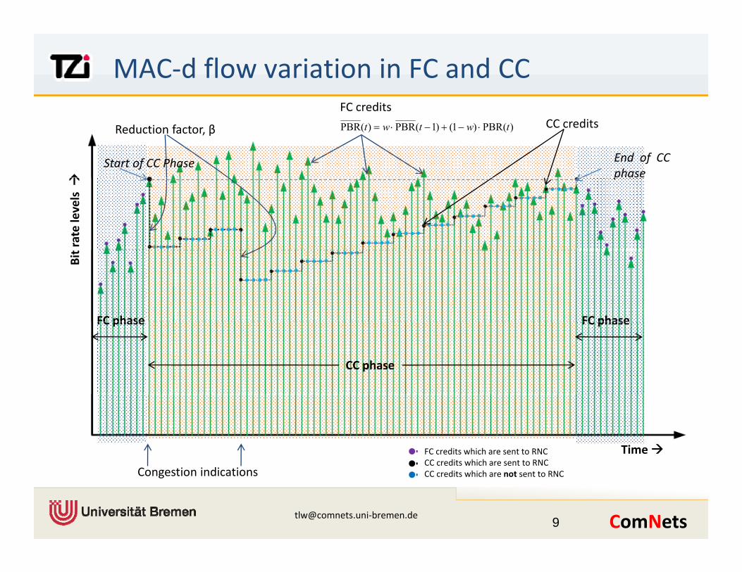
MAC‐d flow variation in FC and CCFC credits

)(PBR)1()1(PBR)(PBR twtwt ⋅−+−⋅=Reduction factor, β

FC credits CC credits

Start of CC Phase End of CC phase

rate levels

p

Bit

FC phaseFC phase

CC phase

FC phaseFC phase

Time FC credits which are sent to RNCCC credits which are sent to RNC


Congestion indications CC credits which are not sent to RNC

Analytical modeling of FC and CC

Prerequisites Two state variables for FC and CC

Time step in CC is several times longer (5) than the time step in FCTime step in CC is several times longer (5) than the time step in FC

Maximum level reached under CC depends on starting FC level

AssumptionsThe interarrival times of CIs are independent and identically distributed

Number of users remains constant (stationary system)Number of users remains constant (stationary system)

Constant transmission delay for CA signals

Per‐user buffer occupancy at Node‐B is not considered for FC modelling


Joint Markov chain

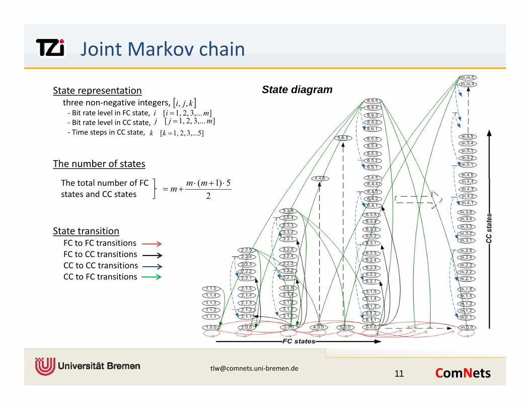
State representationthree non‐negative integers, ‐ Bit rate level in FC state,‐ Bit rate level in CC state, ] 3,... 2, 1,[ mjj =

[ ]kji ,,] 3,... 2, 1,[ mii =

State diagram

‐ Time steps in CC state, ]53,... 2, 1, [ =kk

The number of states

25)1( ⋅+⋅

+=mmmThe total number of FC

states and CC states

State transitionState transitionFC to FC transitionsFC to CC transitionsCC to CC transitionsCC to FC transitions


Markov model: input parameters

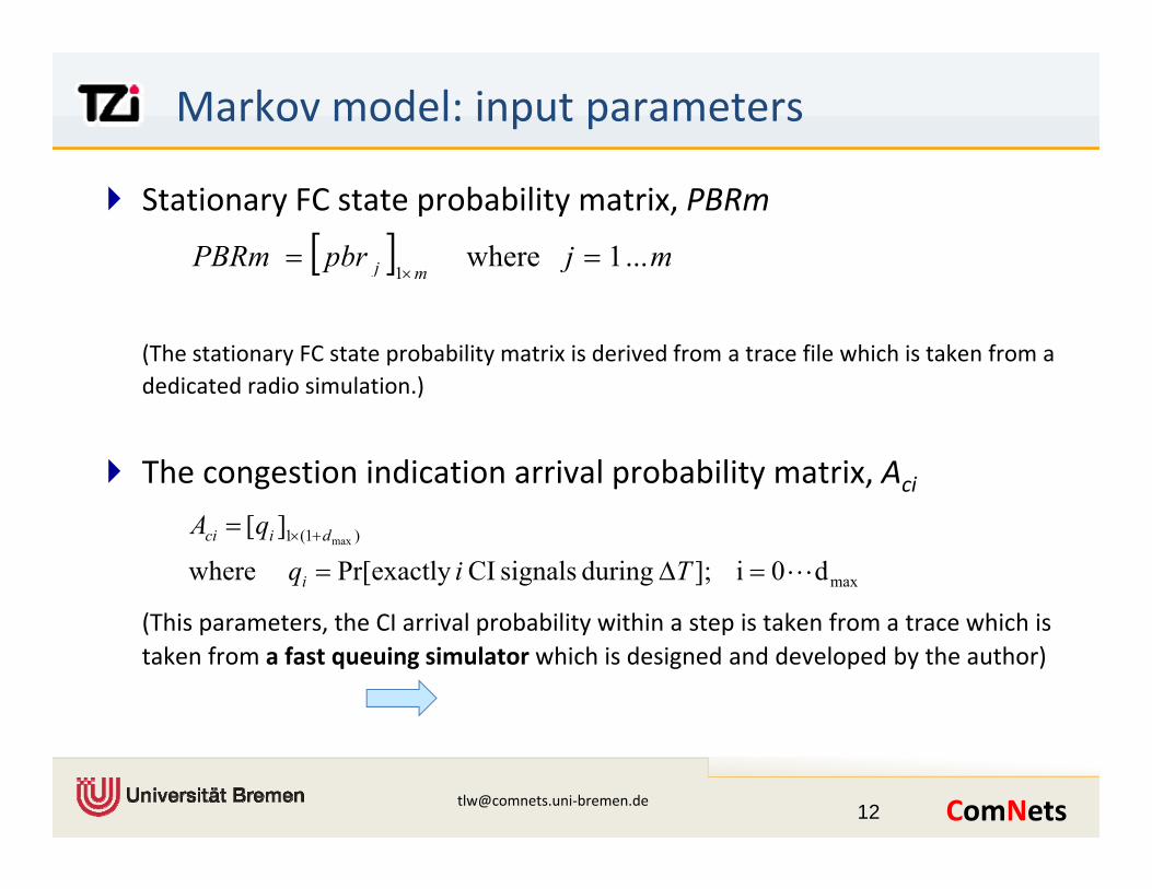
Stationary FC state probability matrix, PBRm

[ ] mjpbrPBRmmj ...1where

1==

×

(The stationary FC state probability matrix is derived from a trace file which is taken from a dedicated radio simulation )

mj 1×

dedicated radio simulation.)

The congestion indication arrival probability matrix, Aci

( h h l b b l h k f h h

max

)1(1

d0i]; during signals CI exactly Pr[ where

][max

L=Δ=

= +×

Tiq

qA

i

dici

(This parameters, the CI arrival probability within a step is taken from a trace which is taken from a fast queuing simulator which is designed and developed by the author)


Transition probability calculations

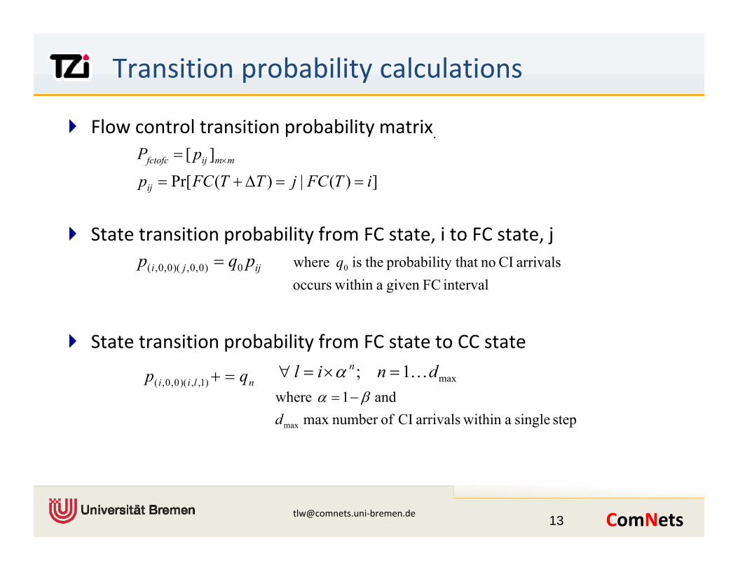
Flow control transition probability matrix.

])(|)(P [

][

iTFCjTTFC

pP mmijfctofc

Δ

= ×

State transition probability from FC state, i to FC state, j

])(|)(Pr[ iTFCjTTFCpij ==Δ+=

ijji pqp 0)0,0,)(0,0,( =interval FCgiven a within occurs

arrivals CI noy that probabilit theis where 0q

State transition probability from FC state to CC state

d1h β )1,,)(0,0,( nlii qp =+ max1; dnil n K=×=∀ α

step single a within arrivals CI ofnumber max and1 where

maxdβα −=


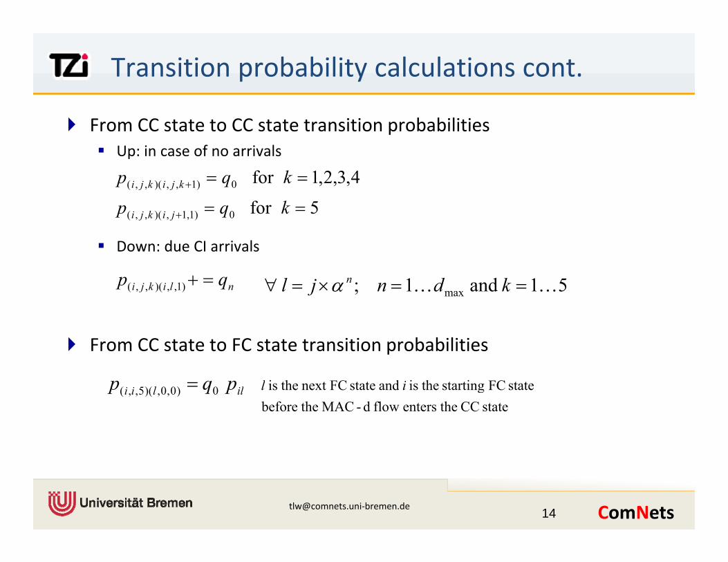
Transition probability calculations cont.

From CC state to CC state transition probabilitiesUp: in case of no arrivals

4321for k

Down: due CI arrivals

5for

4,3,2,1for

0)1,1,)(,,(

0)1,,)(,,(

==

==

+

+

kqp

kqp

jikji

kjikji

Down: due CI arrivals

)1,,)(,,( nlikji qp =+ 51 and 1; max KK ==×=∀ kdnjl nα

From CC state to FC state transition probabilities

illii pqp 0)00)(5( = stateFCstartingtheisandstateFCnexttheis ilillii pqp 0)0,0,)(5,,(state CC theenters flow d-MAC thebefore

stateFCstarting theisandstateFCnext theis il


State probabilities and average throughput

Transition probability matrix, with square dimension nt

[ ]tt nnijkpP

×= fcni

321

,....,3,2,1 where =

Stationary state probabilities matrix

tt nnj ×

st

cc

nknj

,....,3,2,1 ,....,3,2,1

==

πStationary state probabilities matrix,

] ......, , , ,[ vector,state thedenotes πWhere 3210 tnπππππ

πPππ ⋅=

Average throughput sec/1

bitipSizebitRateStetn

ii∑

=

×= π

Example, size of the bit rate level is 33.6 kbps for the given consideration


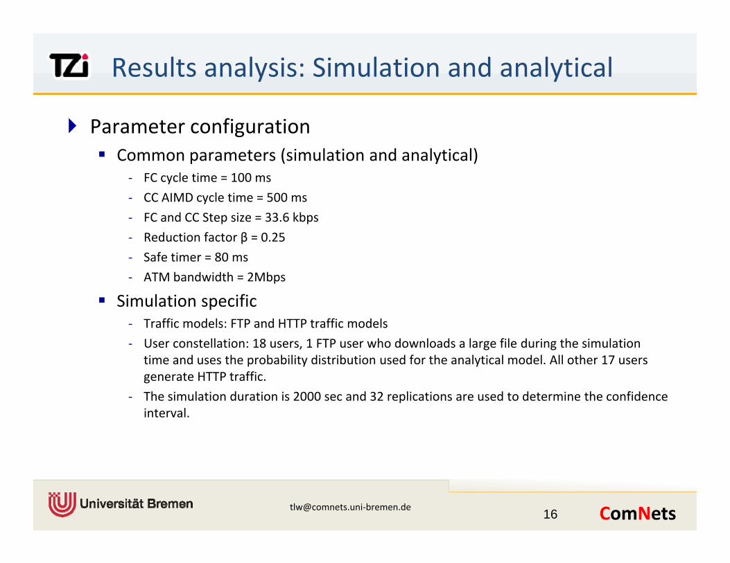
Results analysis: Simulation and analytical

Parameter configurationCommon parameters (simulation and analytical)

FC l ti 100‐ FC cycle time = 100 ms

‐ CC AIMD cycle time = 500 ms

‐ FC and CC Step size = 33.6 kbps

‐ Reduction factor β = 0.25

‐ Safe timer = 80 ms

‐ ATM bandwidth = 2Mbps

Simulation specific‐ Traffic models: FTP and HTTP traffic models

‐ User constellation: 18 users, 1 FTP user who downloads a large file during the simulation time and uses the probability distribution used for the analytical model. All other 17 users generate HTTP traffic.

‐ The simulation duration is 2000 sec and 32 replications are used to determine the confidence interval.


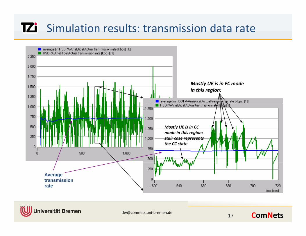
Simulation results: transmission data rate

Mostly UE is in FC mode in this region:

Mostly UE is in CC mode in this region:mode in this region: stair case represents the CC state

Average transmission rate


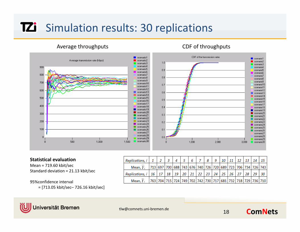
Simulation results: 30 replicationsAverage throughputs CDF of throughputs

Statistical evaluation

iY

iY

Statistical evaluationMean = 719.60 kbit/secStandard deviation = 21.13 kbit/sec

95%confidence interval = [713.05 kbit/sec– 726.16 kbit/sec]


[ / / ]

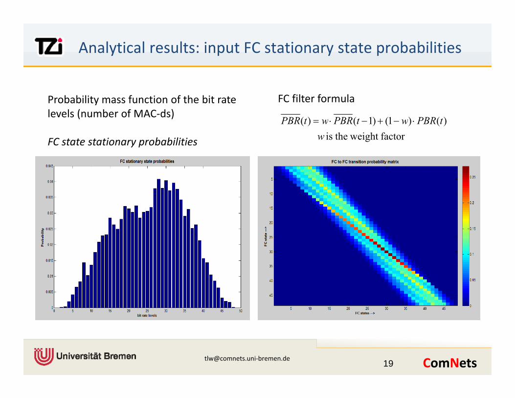
Analytical results: input FC stationary state probabilities

)()1()1()( tPBRwtPBRwtPBR ⋅−+−⋅=

FC filter formulaProbability mass function of the bit rate levels (number of MAC‐ds)

factor weight theis )()1()1()(

wtPBRwtPBRwtPBR +

FC state stationary probabilities


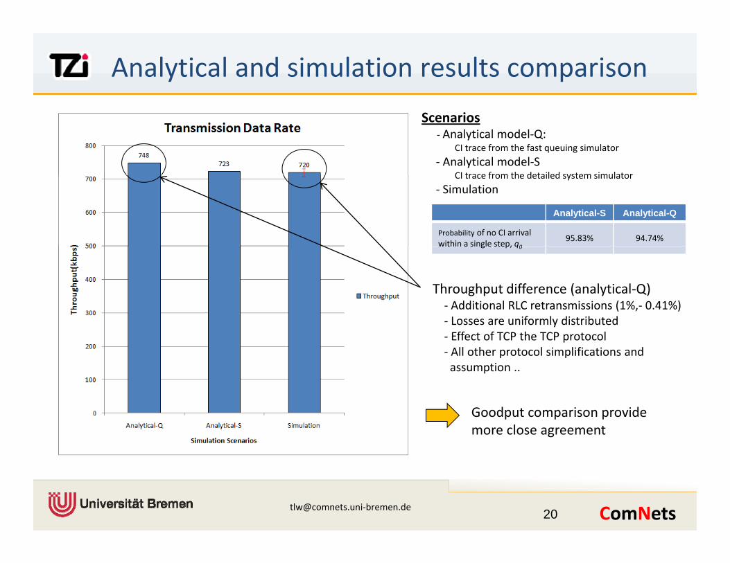
Analytical and simulation results comparison

Scenarios‐ Analytical model‐Q:

CI trace from the fast queuing simulator

‐ Analytical model‐SCI trace from the detailed system simulatorCI trace from the detailed system simulator

‐ Simulation

Analytical-S Analytical-Q

Probability of no CI arrival within a single step, q0

95.83% 94.74%

Throughput difference (analytical‐Q)‐ Additional RLC retransmissions (1%,‐ 0.41%)L if l di ib d

within a single step, q0

‐ Losses are uniformly distributed‐ Effect of TCP the TCP protocol‐ All other protocol simplifications and assumption ..

Goodput comparison provide more close agreement


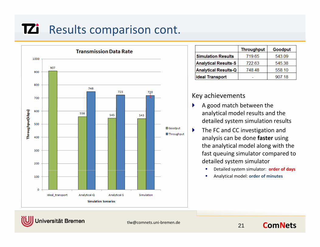
Results comparison cont.

Key achievementsA good match between the ganalytical model results and the detailed system simulation results

The FC and CC investigation and analysis can be done faster usinganalysis can be done faster using the analytical model along with the fast queuing simulator compared to detailed system simulator

Detailed system simulator: order of daysDetailed system simulator: order of days

Analytical model: order of minutes


Conclusion

Detailed HSPA system simulator has been implemented, tested, validated and used for the performance evaluation.

TNL credit‐based adaptive flow control and congestion algorithms have been implemented tested, validated and used for end‐to‐end performance analysis.p y

Overall network performance can be significantly improved by reducing burstiness over the transport network, optimising transport utilisation and effectively minimising congestion in the transport network

FC and CC algorithms provides guaranteed end‐user QoS while achieving a optimum end‐user performance

Two analytical models has been implemented, tested, validated and evaluated the performance.

A Markov model for modelling congestion control functionality

A joint Markov model for modelling FC and CC functionalities


A joint Markov model for modelling FC and CC functionalities

Conclusion

There is a good match between analytical model results and the detailed system simulation results.

A complete faster alternative solution to the timing consuming detailed system simulator can be provided by the analytical mode along with the fast queuing for TNL feature analysis.g q g y

Detailed LTE system simulator implemented, tested, validated and performance analysed.

dd l l l h d l dIn addition to general protocol implementation, MAC scheduler and transport QoS packet scheduler have been implemented

Effects of transport congestion for network and end‐user performance have been studied and analysedstudied and analysed


Outlook

Proper flow control and congestion control schemes are needed to be proposed and implemented in the LTE UTRAN in order to

t t t t k t l d t tiprotect transport packet losses due to congestionUL congestion control and load balancing for non‐GBR bearers

DL congestion handling mainly for non‐GBR bearers

Effective admission control mechanism for GBR bearers

There is a clear requirement of cross layer functionalities between Radio MAC scheduler and transport scheduler for peffective QoS management


Thank you very much!Thank you very much!

Any Questions?


Design overview of the queuing simulator


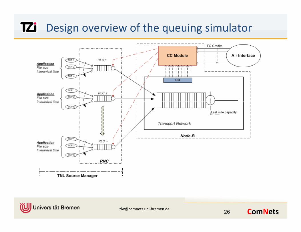
Fast queuing simulator

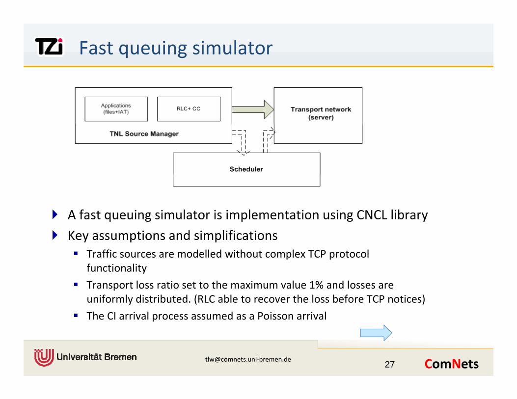
A fast queuing simulator is implementation using CNCL library

Key assumptions and simplificationsTraffic sources are modelled without complex TCP protocol functionality

Transport loss ratio set to the maximum value 1% and losses are uniformly distributed. (RLC able to recover the loss before TCP notices)

The CI arrival process assumed as a Poisson arrival


FC Queue management

(from RNC) Incoming flow )(

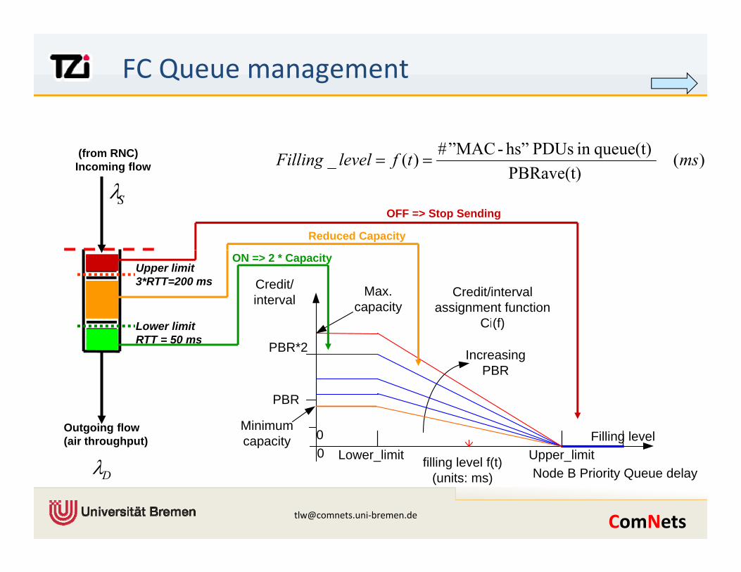
PBRave(t) queue(t)in PDUs hs”-”MAC#)(_ mstflevelFilling ==

SλPBRave(t)

OFF => Stop Sending

Reduced Capacity

Upper limit 3*RTT=200 ms

L li it

Credit/interval Credit/interval

assignment function Ci(f)

Max.capacity

ON => 2 * Capacity

Lower limit RTT = 50 ms

Ci(f)

PBR*2 Increasing PBR

Outgoing flow (air throughput)

λ0

PBR

Filling levelLower_limit Upper_limitfilling level f(t)

0Minimum capacity


Dλ Node B Priority Queue delayfilling level f(t)

(units: ms)

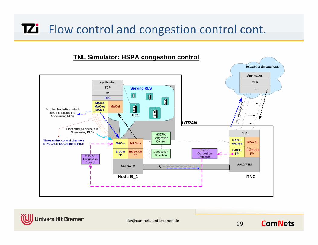
Flow control and congestion control cont.

Application

TNL Simulator: HSPA congestion controlInternet or External User

Uu Interface

Application

TCP

IP

RLC

MAC-dMAC-dMAC-es

Serving RLS IP

TCP

Application

tions

MAC dMAC esMAC-e

RLCHSDPACongestion

UE1To other Node-Bs in which

the UE is located their Non-serving RLSs

RAB

con

nect

From other UEs who is in Non-serving RLSs

UTRAN

MAC-e MAC-hs

E-DCH FP

HS-DSCH FP

AAL2/ATM

MAC-dMAC-es MAC-d

E-DCH FP

HS-DSCH FP

AAL2/ATM

Congestion Detection

Congestion Control

HSUPACongestion

Control

HSUPACongestion Detection

Three uplink control channels E-AGCH, E-RGCH and E-HICH

RNCNode-B_1


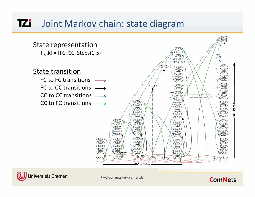
Joint Markov chain: state diagram

State representation[i,j,k] = [FC, CC, Steps(1‐5)]

State transitionFC to FC transitionsFC t CC t itiFC to CC transitionsCC to CC transitionsCC to FC transitions


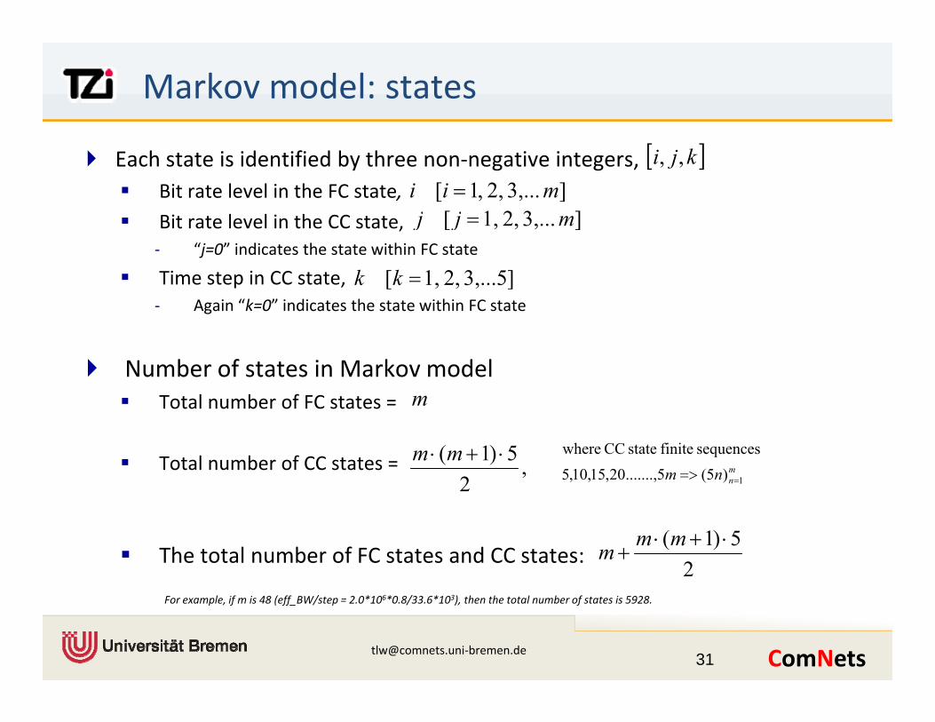
Markov model: states

Each state is identified by three non‐negative integers, Bit rate level in the FC state,

Bit rate level in the CC state

[ ]kji ,,] 3,... 2, ,1[ mii =

]3,...2,1,[ mjj =Bit rate level in the CC state, ‐ “j=0” indicates the state within FC state

Time step in CC state, ‐ Again “k=0” indicates the state within FC state

] 3,...2,1,[ mjj

]53,... 2, 1, [ =kk

Number of states in Markov modelTotal number of FC states = mTotal number of FC states

Total number of CC states = ,2

5)1( ⋅+⋅ mmmnnm 1)5(5.......,20,15,10,5

sequences finite state CC where

==>

The total number of FC states and CC states: 25)1( ⋅+⋅

+mmm


For example, if m is 48 (eff_BW/step = 2.0*106*0.8/33.6*103), then the total number of states is 5928.

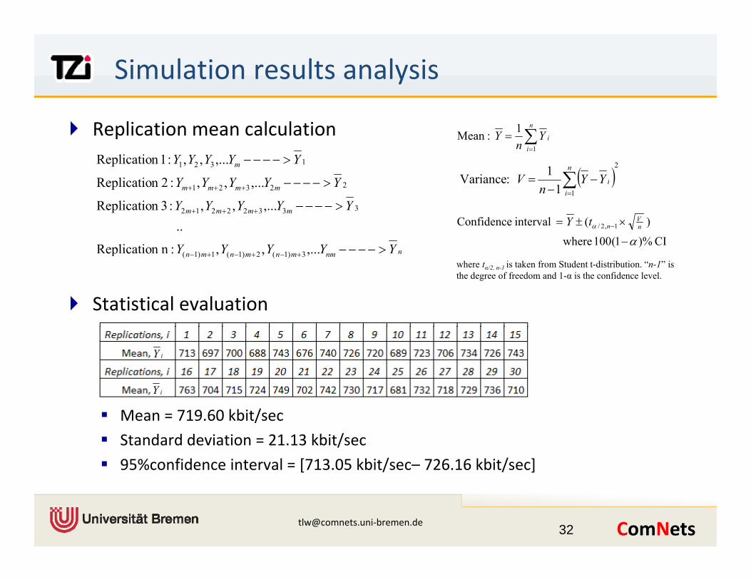
Simulation results analysis

Replication mean calculation

m

YYYYY

YYYYY

>

>−−−−

2R li ti

,...,,:1n Replicatio 1321

∑=

=n

iiY

nY

1

1 :Mean

( )21:Variance ∑ −=

n

iYYV

nnmmnmnmn

mmmm

mmmm

YYYYY

YYYYY

YYYYY

>−−−−

>−−−−

>−−−−

+++

+++

+++

,...,,:nn Replicatio

..,...,,:3n Replicatio

,...,,:2n Replicatio

3)1(2)1(1)1(

33322212

22321( )

11 :Variance ∑

=−=

iiYY

nV

CI )%1(100 where

) ( interval Confidence 1,2/

αα

−

×±= − nV

ntY

Statistical evaluation

nnmmnmnmn +−+−+− ,...,,:ep c o 3)1(2)1(1)1(where tα/2, n-1 is taken from Student t-distribution. “n-1” is the degree of freedom and 1-α is the confidence level.

iY

iY

Mean = 719.60 kbit/sec

Standard deviation = 21.13 kbit/sec

95%confidence interval = [713.05 kbit/sec– 726.16 kbit/sec]


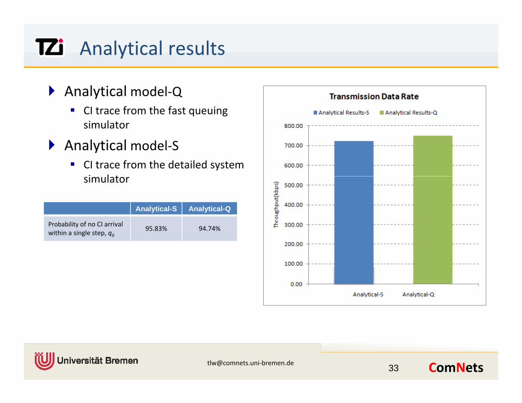
Analytical results

Analytical model‐QCI trace from the fast queuing simulatorsimulator

Analytical model‐SCI trace from the detailed system i l tsimulator

Analytical-S Analytical-Q

Probability of no CI arrival 95 83% 94 74%

ywithin a single step, q0

95.83% 94.74%


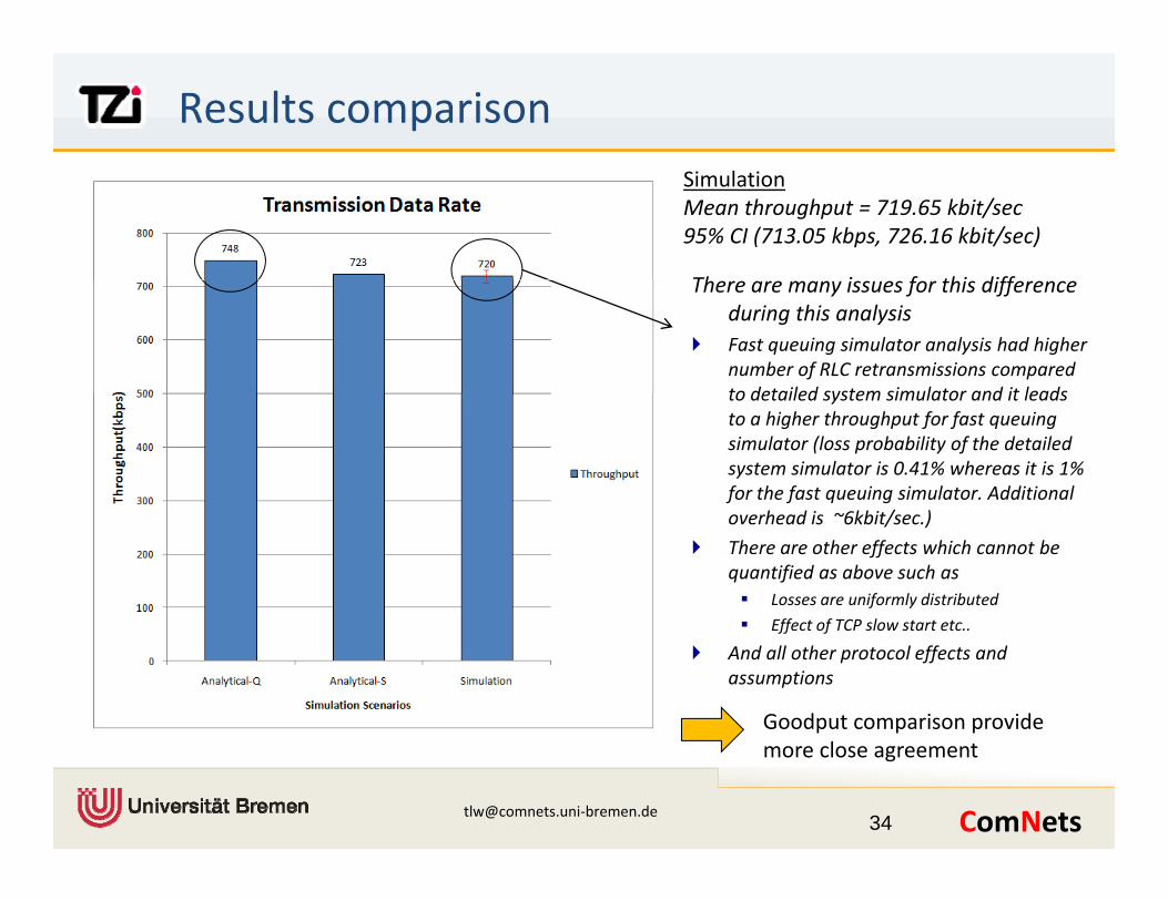
Results comparison

Th i f thi diff

SimulationMean throughput = 719.65 kbit/sec95% CI (713.05 kbps, 726.16 kbit/sec)

There are many issues for this difference during this analysisFast queuing simulator analysis had higher number of RLC retransmissions compared to detailed system simulator and it leadsto detailed system simulator and it leads to a higher throughput for fast queuing simulator (loss probability of the detailed system simulator is 0.41% whereas it is 1% for the fast queuing simulator. Additional overhead is ~6kbit/sec.)

There are other effects which cannot be quantified as above such as

Losses are uniformly distributed

Eff t f TCP l t t tEffect of TCP slow start etc..

And all other protocol effects and assumptions

Goodput comparison provide


more close agreement

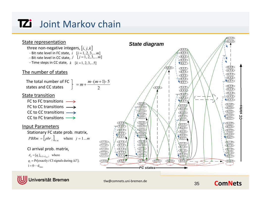
Joint Markov chain

State representationthree non‐negative integers, ‐ Bit rate level in FC state,‐ Bit rate level in CC state,Time steps in CC state

] 3,... 2, 1,[ mjj =]5321[kk

[ ]kji ,,] 3,... 2, 1,[ mii =

State diagram

‐ Time steps in CC state, ]53,...2,1, [ =kk

The number of states

25)1( ⋅+⋅

+=mmmThe total number of FC

states and CC states 2states and CC states

State transitionFC to FC transitionsFC to CC transitionsCC to CC transitionsCC to CC transitionsCC to FC transitions

Input ParametersStationary FC state prob. matrix,

[ ] mjpbrPBRm 1where ==

CI arrival prob. matrix,

[ ] mjpbrPBRmmj ...1where

1==

×

)1(1

]; during signals CI exactly Pr[

where][max

Δ=

= +×

Tiq

qA

i

dici


maxd0i L=

Documents

Oti i tiOptimization and PfP erformance Analysis of High ... · Not backward compatible with previous UMTS. HSPA architecture (UMTS, HSDPA, HSUPA) UE: User Equipment USIM: ... q i