Embed Size (px)
Citation preview

i
Digitally Signed by: Content manager’s Name
DN : CN = Webmaster’s name
O = University of Nigeria, Nsukka
OU = Innovation Centre
Agboeze Irene E.
ENGINEERING
ELECTRICAL ENGINEERING
THERMAL MODELLING OF INDUCTION
MACHINE USING THE LUMPED PARAMETER
MODEL
OTI, STEPHEN EJIOFOROTI, STEPHEN EJIOFOROTI, STEPHEN EJIOFOROTI, STEPHEN EJIOFOR
REG. NO: PG/PH.D/07/42465REG. NO: PG/PH.D/07/42465REG. NO: PG/PH.D/07/42465REG. NO: PG/PH.D/07/42465

ii
THERMAL MODELLING OF INDUCTION THERMAL MODELLING OF INDUCTION THERMAL MODELLING OF INDUCTION THERMAL MODELLING OF INDUCTION MMMMACHINE ACHINE ACHINE ACHINE
USING THE LUMPED PARAMETER MODELUSING THE LUMPED PARAMETER MODELUSING THE LUMPED PARAMETER MODELUSING THE LUMPED PARAMETER MODEL....
BYBYBYBY
OTI, STEPHEN EJIOFOROTI, STEPHEN EJIOFOROTI, STEPHEN EJIOFOROTI, STEPHEN EJIOFOR
REG. NO: PG/PH.D/07/42465REG. NO: PG/PH.D/07/42465REG. NO: PG/PH.D/07/42465REG. NO: PG/PH.D/07/42465
DEPARTMENT OF ELECTRICAL ENGINEERINGDEPARTMENT OF ELECTRICAL ENGINEERINGDEPARTMENT OF ELECTRICAL ENGINEERINGDEPARTMENT OF ELECTRICAL ENGINEERING
UNIVERSITY OF NIGERIA, NSUKKAUNIVERSITY OF NIGERIA, NSUKKAUNIVERSITY OF NIGERIA, NSUKKAUNIVERSITY OF NIGERIA, NSUKKA
DECDECDECDECEEEEMBERMBERMBERMBER, 20, 20, 20, 2011114444....
SUPERVISORS: PROF. M. U. AGU & PROF. E. C. EJIOGU

iii
THERMAL MODELLING OF INDUCTION MACHINE
USING THE LUMPED PARAMETER MODEL
A THESIS SUBMITTED IN PARTIAL FULFILLMENT OF THE
REQUIREMENT FOR THE AWARD OF DOCTOR OF PHILOSOPHY
(Ph.D) DEGREE IN ELECTRICAL ENGINEERING DEPARTMENT,
UNIVERSITY OF NIGERIA, NSUKKA
BY
OTI, STEPHEN EJIOFOR
REG. NO: PG/Ph.D/07/42465
UNDER THE SUPERVISION
OF
ENGR. PROF. M. U. AGU & ENGR. PROF. E. C. EJIOGU
DEPARTMENT OF ELECTRICAL ENGINEERING
UNIVERSITY OF NIGERIA, NSUKKA
DECEMBER, 2014.

iv
TITLE PAGE
THERMAL MODELLING OF INDUCTION MACHINE USING THERMAL MODELLING OF INDUCTION MACHINE USING THERMAL MODELLING OF INDUCTION MACHINE USING THERMAL MODELLING OF INDUCTION MACHINE USING
THE LUMPED PARAMETER MODELTHE LUMPED PARAMETER MODELTHE LUMPED PARAMETER MODELTHE LUMPED PARAMETER MODEL
v
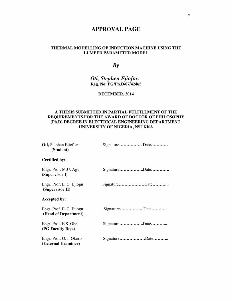
APPROVAL PAGE
THERMAL MODELLING OF INDUCTION MACHINE USING THE
LUMPED PARAMETER MODEL
By
Oti, Stephen Ejiofor. Reg. No: PG/Ph.D/07/42465
DECEMBER, 2014
A THESIS SUBMITTED IN PARTIAL FULFILLMENT OF THE
REQUIREMENTS FOR THE AWARD OF DOCTOR OF PHILOSOPHY
(Ph.D) DEGREE IN ELECTRICAL ENGINEERING DEPARTMENT,
UNIVERSITY OF NIGERIA, NSUKKA
Oti, Stephen Ejiofor: Signature……………. Date…………
(Student)
Certified by:
Engr. Prof. M.U. Agu Signature……………..Date………….
(Supervisor I)
Engr. Prof. E. C. Ejiogu Signature………………Date………...
(Supervisor II)
Accepted by:
Engr. Prof. E. C. Ejiogu Signature……………..Date………...
(Head of Department)
Engr. Prof. E.S. Obe Signature……………..Date………...
(PG Faculty Rep.)
Engr. Prof. O. I. Okoro Signature………………Date………..
(External Examiner)
vi
CERTIFICATION PAGE
I hereby certify that the work which is being presented in this thesis entitled,
“Thermal Modelling of Induction Machine Using the Lumped Parameter Model”, in
partial fulfillment of the requirements for the award of Doctor of Philosophy (Ph.D)
Degree (Electric Machines & Drives) in the Department of Electrical Engineering,
University of Nigeria, Nsukka is an authentic record of the research carried out under
the supervision of Engr. Prof. M.U. Agu and Engr. Prof. E. C. Ejiogu except where
due reference has been made in the work. Therefore, opinions and assertions
contained herein are those of the authors as they are indicated on the reference pages.
The work embodied in this thesis has not been submitted for the award of any degree
of any other University.
Oti, Stephen Ejiofor: Signature……………. Date…………
(Student)
This is to certify that the above statement made by the candidate is correct and true to
the best of my knowledge.
Engr. Prof. M.U. Agu Signature……………..Date………….
(Supervisor I)
Engr. Prof. E. C. Ejiogu Signature………………Date………..
(Supervisor II)
Accepted by:
Engr. Prof. E. C. Ejiogu Signature……………..Date………...
(Head of Department)
Engr. Prof. E.S. Obe Signature……………..Date………...
(PG Faculty Rep.)
Engr. Prof. O. I. Okoro Signature………………Date………..
(External Examiner)

vii
DEDICATION
To godfathers that have the fear of God in them.

viii
ACKNOWLEDGEMENT
I am heartily thankful to my supervisors, Engr. Prof. M.U. Agu and Engr.
Prof. E.C. Ejiogu whose encouragement, guidance and support enabled
me to develop an understanding of the subject.
I would like to express my profound gratitude to Ven. Prof. T.C.
Madueme, Prof. L.U. Anih and Dr. B.O. Anyaka for their warm advice
and useful contributions, all towards making this work a success.
At the early stage of this work, and all the way from Germany, Dr. E.S.
Obe (now Professor) bombarded me with journal materials that I had
more than I needed. This similar feat was repeated of recent by Engr.
Chukwuemeka Awah who travelled out for his doctoral programme. May
God reward you abundantly.
I owe my deepest gratitude to Professor O.I. Okoro, who has been with
me physically and spiritually since the inception of this work, if it gives a
farmer joy as the planted seeds sprout, how much is expected of men
builder in the person of Prof. Okoro?
I am indebted to many of my colleagues: Engrs. Nwosu, Nnadi, Odeh,
Ogbuka, Mbunwe and Ani who have shared with me or supported me in
one way or the other to make or mar me. May God bless all of them.
It is an honour for me to thank the men at the laboratory unit- Mr.
Okafors, Okoro, Abula, Azu , Eze and Chi for their usual cooperation.
Emeka Omeje is also remembered for his prompt response when his
attention is needed by me. Many thanks to my friends: Hacco, Chika,
Okpoko, Chibuzo, Steve Agada, Alex, Simon, Ejor, Moses, Emma
Obollor, Amoke and Engr. Agbo of Mechanical Engineering.
At this juncture, I have to thank my people; brother Mike, sister Uche,
Uncle Emma, Amara and Princess for enduring with us until now that
God has chosen, and to Him be the Glory.
Lastly, I offer my regards and blessings to all of those who supported me
in any respect during the completion of the project.

ix
Abstract
Temperature rise is of much concern in the short and long term
operations of induction machine, the most useful industrial work icon.
This work examines induction machines mean temperatures at the
different core parts of the machine. The system’s thermal network is
developed, the algebraic and differential equations for the proposed
models are solved so as to ascertain the thermal performances of the
machine under steady and transient conditions. The lumped parameter
thermal method is used to estimate the temperature rise in induction
machine. This method is achieved using thermal resistances, thermal
capacitances and power losses. To analyze the thermal process, the
7.5kW machine is divided geometrically into a number of lumped
components, each component having a bulk thermal storage and heat
generation and interconnections to adjacent components through a
linear mesh of thermal impedances. The lumped parameters are derived
entirely from dimensional information, the thermal properties of the
materials used in the design, and constant heat transfer coefficients.
The thermal circuit in steady-state condition consists of thermal
resistances and heat sources connected between the components nodes
while for transient analysis, the thermal capacitances were used
additionally to take into account the change in internal energy of the
body with time. In the course of the simulation using MATLAB, the
response curves showing the predicted temperature rise for the
induction machine core parts were obtained. To find out the effect of
the decretization level on the symmetry, the two different thermal
models, the SIM and the LIM models having eleven and thirteen nodes
respectively were considered and the results from the two models were
compared. The resulting predicted temperature values together with
other results obtained in this work provide useful information to
designers and industries on the thermal characteristics of the induction
machine.

x
TABLE OF CONTENTS
Title page ………………………………………………………....…………….....….iii
Approval page ………………………………………………………………....….…..iv
Certification page………………………………………………………….…..….…...v
Dedication page…………………………………………………………….…..….…..vi
Acknowledgement………………………………………………………….…..….….vii
Abstract……………………………………………………………………..…..….….viii
Table of contents…………………………………………………….….……..….…...ix
List of figures…………………………………………………………….……..……..xii
List of tables………………………………………………………….…….…..….….xiv
List of symbols…………..……………………………………….……………..……..xv
Chapter One: INTRODUCTION ………………………………………………..….…..1
1.1 Background of study…………….……………….…………………………....…1
1.2 Statement of Problem …………………..……….…………….……….….….…3
1.3 Purpose of Study ………………………………..……………..........................3
1.4 Significance of Study …………………………...…………….………………....4
1.5 Scope of Study..…………………………………...….…..................................5
1.6 Arrangement of Chapters ……..………………………………….…................5
Chapter Two: LITERATURE REVIEW …………………………….……………….....6
Chapter Three: HEAT TRANSFER MECHANISMS IN ELECTRICAL MACHINES
3.1 Heat Transfer in Electrical Machines…………….……………….….…......12
3.2 Modes of Heat Transfer …………………..……………..…….………….…13
3.2.1 Conduction ………………………………………………….………...............14
3.2.2 Convection ……………………………………………...……………………..16
3.2.3 Radiation …………………..…………………………………….…................18
3.3. Heat Flow in Electrical Machines ………………….…………..……..…..…20
3.3.1 Heat Transfer Flow Types …………………………………………………..20

xi
3.3.2 Heat Transfer Flow System …………………………………..……….……..21
3.3.3 The Boundary Layers……………………………………...……….…………22
3.4 Determination of Thermal Conductance…………………….......….……....23
3.5 Thermal-Electrical Analogous Quantities ………………………….….……25
3.5.1 Thermal and Electrical Resistance Relationship …………….….…..…….26
Chapter Four: THERMAL MODEL DEVELOPMENT AND PARAMETER COMPUTATION
4.1 Cylindrical Component and Heat Transfer Analysis…………….………......28
4.2 Conductive Heat Transfer Analysis in Induction Motor ………….…….…...28
4.3 Convective Heat Transfer Analysis in Induction Motor………….…….…....34
4.4 Description of Model Components and Assumptions …………….…….….35
4.5 Calculation of Thermal Resistances…………………………….………...….45
4.6 Calculation of Thermal Capacitances ………………………..…………....…56
Chapter Five: LOSSES IN INDUCTION MACHINE
5.1 Determination of Losses in Induction Motors .…………………….…........69
5.1.1 Stator and Rotor Copper Losses ……………………..…………….…….. 69
5.1.2 Core Losses …………………………………………….…….……..….……70
5.1.3 Friction and Windage Losses ………………………….………..………….70
5.1.4 Differential Flux Densities and Eddy-Currents in the Rotor Bars ………..71
5.1.5 Stray-Load Losses …………………………………………………………....72
5.1.6 Rotor Copper Losses ……………………………………………...…….…...72
5.1.7 No Load Losses …………………………………………….…………….…..73
5.1.8 Pulsation Losses ……………………………………………………………...74
5.2 Calculation of Losses from IM Equivalent Circuit…………………………..74
5.3 Loss Estimation of the 7.5 kW Induction machine ….….………………....79
5.4 Segregation and Analysis of the IM Losses……… …………………........82
5.5 Performance Characteristics of the 10 HP Induction machine…..…….....83
5.6.1 Motor Efficiency /Losses ……………………….……………………….......86

xii
5.6.2 Determination of Motor Efficiency ……………………..……...….…….......86
5.6.3 Improving Efficiency by Minimizing Watts Losses ……………………......87
5.7 The Effects of Temperature ……………………………..….…….…...........88
Chapter Six: THERMAL MODELLING AND COMPUTER SIMULATION
6.1 The Heat Balance Equations …………………………………................…...90
6.2 Thermal Models and Network Theory ……………...……………….….....…90
6.3 The Transient State Analysis ……………………………….………....……...98
6.4 The Steady State Analysis …………………………………………………..104
6.5 Transient State Analysis results.………………….….……...………..……..108
6.6 Discussion of Results …………………………….…………...………..…….116
Chapter Seven: CONCLUSION AND RECOMMENDATION
7.1 Conclusion…………………….……………….….…………...………..…….118
7.2 Recommendation …………….………………….…………...………..…….119
REFERENCES …………………………………………………………………..…..….…..120
APPENDIX……...………………………………………..……………….……..……….…..131

xiii
LIST OF FIGURES
Figure 3.1: Illustration of Fourier’s Conduction Law 15
Figure 3.2: Illustration of Newton’s law of cooling 16
Figure 3.3: Simplified diagram for the illustration of thermal and
electrical resistance relationship 26
Figure 3.4: Simplified diagram for further illustration of thermal and
electrical equivalent resistance 27
Figure 4.1: Heat transfer mechanism in squirrel cage IM 28
Figure 4.2: General cylindrical component 28
Figure 4.3: Conductive Thermal circuit- An annulus ring 29
Figure 4.4: Three terminal networks of the axial and radial networks 30
Figure 4.5: The combination of axial and radial networks for a symme-
trically distributed temp about the central radial plane. 32
Figure 4.6: Squirrel Cage Induction Machine Construction 36
Figure 4.7: The geometry of High Speed Induction Machine 36
Figure 4.8: The geometry of Induction Machine rotor teeth 38
Figure 4.9: Squirrel Cage Rotor 41
Figure 4.10: Thermal network model for the Induction machine 43
Figure 4.11: Thermal resistance of air-gap between insulation and iron 45
Figure 4.12: Thermal resistance between the stator iron and the yoke 47
Figure 4.13: Thermal resistance between stator iron and end-winding 49
Figure 4.14: Thermal resistance between Rotor Bar and end ring 50
Figure 4.15: Thermal capacitance for Stator Lamination 56
Figure 4.16: Thermal capacitance for stator iron 57
Figure 4.17: Thermal capacitances for end winding 59
Figure 4.18: Thermal capacitances for rotor iron 61
Figure 4.19: Thermal capacitances for the Rotor bar 63
Figure 4.20: Thermal Capacitance for the Various Rotor-Bar Sections 64

xiv
Figure 4.21: Thermal capacitances for the End rings 65
Figure 5.1. Equivalent Circuit of the AC induction Machine 75
Figure 5.2. Simplified Equivalent Circuit of the AC induction Machine 75
Figure 5.3. IEEE Equivalent Circuit of the AC induction Machine 76
Figure 5.4. Bar chart for loss segregation of 10HP induction machine 82
Figure 5.5. Graph of Torque-Speed characteristics for 10HP IM 83
Figure 5.6. Power against speed for 10HP induction machine 83
Figure 5.7. Stator current against Speed for 10HP IM 84
Figure 5.8. Graph of Torque-Slip characteristics for 10HP IM 84
Figure 5.9. Power factor against speed for 10HP IM 85
Figure 6.1:Transient Thermal model of SCIM with lumped parameter 91
Figure 6.2:Steady State Thermal model of SCIM with lumped parameter 91
Figure 6.3:Thermal network model for the SCIM (SIM Half Model) 95
Figure 6.4:Thermal network model for the SCIM (LIM Full Model) 97
Figure 6.5: Percentage difference in component steady state temperature for the half and full SIM model 107 Figure 6.6: Percentage difference in component steady state temperature for the half and full LIM model 107
Figure 6.7:Response curve for the predicted temp-(SIM Half Model) 108
Figure 6.8: Response curve for the predicted temp-(SIM Half Model contd.)109
Figure 6.9: Graph for predicted temp and symmetry-(SIM Full Model) 110
Figure 6.10:Response curve for predicted steady state temp for LIM 111
Figure 6.11:Response curve for predicted temp - (LIM Model contd.) 112
Figure 6.12: Graph for predicted steady state temp rise for LIM contd. 113
Figure 6.13: Curves to show symmetry in end-ring of LIM model 114
Figure 6.14: Graph for predicted temp and symmetry-(LIM Full Model) 115

xv
LIST OF TABLES
Table 3.1: Thermal conductivities of some materials at room conditions 15
Table 3.2: Emissivity of some materials at 300K 19
Table 3.3: Thermal-Electrical Analogous Quantities 26
Table 4.1: Machine geometric / Dimensional data 44
Table 4.2: Thermal capacitances and thermal resistances from circuit 68
Table 5.1: Induction machine ratings and parameters 79
Table 5.2: Loss Segregation Obtained from Calculation 82
Table 5.3: Efficiency improvement schemes 88
Table 6.1 Steady State predicted temp for different models 106

xvi
LIST OF SYMBOLS
A area [m2]
bA cross-sectional area of rotor bar [m2]
CuA copper area in a stator slot [m2]
rA cross-sectional area of a rotor end ring [m2]
maxB maximum value of the flux density [T]
b thickness or width [m]
rbb width of rotor bar [m]
dsb stator tooth width [m]
drb rotor tooth width [m]
C heat capacity [J/kg.K]
cuC heat capacity of copper [J/kg.K]
d diameter or thickness [m]
ad air pocket thickness [m]
id slot insulation thickness [m]
f frequency [Hz]
FRIwin friction and windage loss
rG Grashof number
g acceleration due to gravity [m/s2]
h height [m]
ch convective heat transfer coefficient [W/m2K]
yh height of yoke
rbh height of rotor bar [m]
0I no load current [A]
sI stator current [A]
rI rotor current [A]
Fk eddy current loss factor
Hyk hysteresis loss factor
mL magnetizing inductance [H]
avl average conductor length of half a turn [m]
slotL entire slot length [m]
barL length of rotor bar [m]
L stator core length [m]
LIM large induction machine
rl length of a rotor end ring segment [m]

xvii
sL leakage inductance of stator [H]
m phase number of motor phases
sN speed of rotating magnetic flux [rad/s]
rL leakage inductance of rotor [H]
mL magnetizing inductance [H]
M mass [kg]
Nu Nusselt number
P power [W]
cusP resistive losses in the stator winding [W]
curP resistive losses in the rotor winding [W]
FesP stator core losses [W]
fwP losses due to friction and windage [W]
strP stray losses in the rotor [W]
outP output power [W]
inP input power [W]
rP Prandtl number
P number of poles per phase
p number of pole pairs
rN rotor slot number
sN stator slot number
q heat flux [W/m2]
cR core loss resistance [Ω]
thR thermal resistance [K/W]
Re Reynolds number
ROTcuL rotor copper loss [W]
ROTaL rotational loss [W]
mR iron (core) loss resistance [Ω]
sR stator resistance [Ω]
rR rotor resistance [Ω]
inr inner radius of tooth [m]
outr outer radius of tooth [m]
r radius [m]
δr average radius of the air gap [m]
s slip
SIM small induction machine
STAcore stator core loss [W]
STAcuL stator copper loss [W]

xviii
SCIM squirrel cage induction machine
T temperature [oC, K]
qrT torque [Nm]
maxT maximum temperature [oC]
shT shaft torque [Nm]
∞T reference temperature [oC],
pitchT tooth pitch [m]
T∆ temperature drop over the air gap [K]
t time [s] TNM thermal network model
2ν kinematic viscosity [m2/s]
sV Voltage [V]
phV phase voltage [V]
ThV Thevenin voltage [V]
tC thermal capacitance matrix
cuρ density of cooper [Kg/m3]
tG thermal conductance matrix
tP loss vector [W]
tθ temperature vector [K]
θ angle between phase voltage and current [degrees]
α heat transfer coefficient [W/m2K]
β volume coefficient of expansion [1/K]
∆ sheet thickness [m]
slotδ air gap of slot [m]
0δ air gap [m]
sagλ stationary air-gap film coefficient
ragλ rotating air-gap film coefficient
ε emissivity
fT temperature rise of the frame [K]
Feλ thermal expansion coefficient of iron [1/K]
ck thermal conductivity [W/m.K]
airk thermal conductivity of air [W/m.K]
insk thermal conductivity of the slot insulation [W/m.K]
sk thermal conductivity of the slot material [W/m.K]
xk
thermal conductivity in x direction [W/m.K]
µ dynamic viscosity [kg/m.s]

xix
0µ permeability of free space [Vs/Am]
υ kinematic viscosity [m2/s]
ρ density [kg/m3]
eρ resistivity [Ωm]
σ Stefan-Boltzmann’s constant [W/m2k
4]
ω angular speed [rad/s]
sR stator resistance [Ω]
IM induction machine
sI stator current [A]
rI rotor current [A]
sV per phase supply voltage of stator [V]
olV volume
rE opposition emf of the rotor [V]
mI magnetizing current [A]
mX magnetizing reactance [Ω]
LsX leakage reactance of the stator [Ω]
rLX leakage reactance of the rotor [Ω]
sX stator leakage reactance [Ω]
mX magnetizing reactance [Ω]
rX rotor reactance [Ω]
sZ stator impedance [Ω]
rZ rotor impedance [Ω]

1
CHAPTER ONE
INTRODUCTION
1.1 Background of Study
This thesis is concerned with the thermal modelling of the induction
machine. With the increasing quest for miniaturization, energy
conservation and efficiency, cost reduction, as well as the imperative to
exploit easier and available topologies and materials, it becomes
necessary to analyze the induction machine thermal circuit to the same
tone as its electromagnetic design. This would help in achieving an early
diagnosis of thermo-electrical faults in induction machines, leading to an
extensively investigated task which pays back in cost and maintenance
savings. Since failures in induction machines occur as a result of aging of
the machine itself or from severe operating conditions then, monitoring
the machine’s thermal condition becomes crucial so as to detect any fault
at an early stage thereby eliminating catastrophic machine faults and
avoidance of expensive maintenance costs. Faults in induction machines
can be broadly classified into thermal faults, electrical faults and
mechanical faults. Currently, stator electrical faults are mitigated by recent
improvements in the design and manufacture of stator windings. However,
in case of machine driven by switching power converters the machine is
stressed by voltages including high harmonic contents. The latter option is
becoming the standard for electric drives. A solution is the development of
vastly improved thermal system cum insulation material. On the other side,
cage rotor design is receiving slight modifications, apart from that, rotor
bars breakage can be caused by thermal stress, electromagnetic forces,
electromagnetic noise and vibration, centrifugal forces, environmental
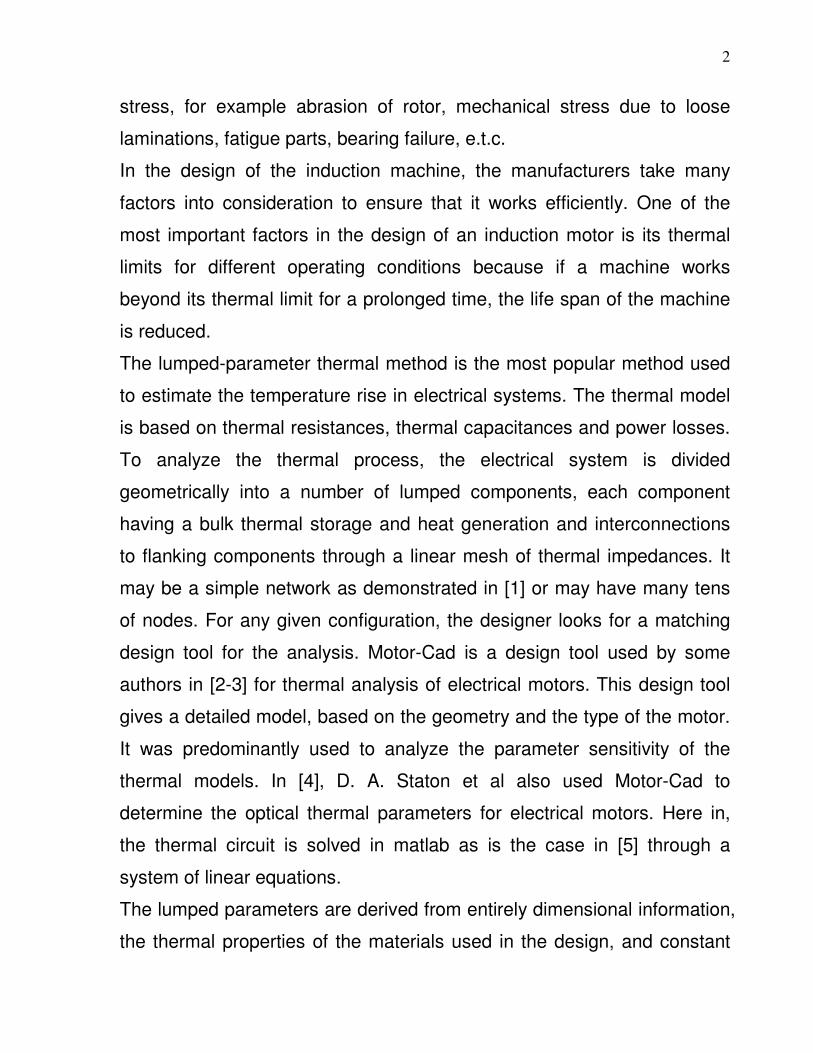
2
stress, for example abrasion of rotor, mechanical stress due to loose
laminations, fatigue parts, bearing failure, e.t.c.
In the design of the induction machine, the manufacturers take many
factors into consideration to ensure that it works efficiently. One of the
most important factors in the design of an induction motor is its thermal
limits for different operating conditions because if a machine works
beyond its thermal limit for a prolonged time, the life span of the machine
is reduced.
The lumped-parameter thermal method is the most popular method used
to estimate the temperature rise in electrical systems. The thermal model
is based on thermal resistances, thermal capacitances and power losses.
To analyze the thermal process, the electrical system is divided
geometrically into a number of lumped components, each component
having a bulk thermal storage and heat generation and interconnections
to flanking components through a linear mesh of thermal impedances. It
may be a simple network as demonstrated in [1] or may have many tens
of nodes. For any given configuration, the designer looks for a matching
design tool for the analysis. Motor-Cad is a design tool used by some
authors in [2-3] for thermal analysis of electrical motors. This design tool
gives a detailed model, based on the geometry and the type of the motor.
It was predominantly used to analyze the parameter sensitivity of the
thermal models. In [4], D. A. Staton et al also used Motor-Cad to
determine the optical thermal parameters for electrical motors. Here in,
the thermal circuit is solved in matlab as is the case in [5] through a
system of linear equations.
The lumped parameters are derived from entirely dimensional information,
the thermal properties of the materials used in the design, and constant

3
heat transfer coefficients. The thermal circuit in steady-state condition
consists of thermal resistances and heat sources connected between the
components nodes while for transient analysis, the heat thermal
capacitances are used additionally to take into account the change in
internal energy of the body with time. The associated equivalent thermal
network, would have the heat generation in the component concentrated
in its midpoint. This point represents the mean temperature of the
component.
1.2 Statement of Problem
The main limiting factor for how much an electric machine can
continuously be loaded is usually the temperature. When a machine
exceeds its thermal limit there are various outcomes: The oxidation
process in insulation materials is accelerated, which eventually leads to
loss of dielectric property. Bearing lubricants may deteriorate or the
viscosity may become too high, resulting in reduced oil film thickness.
Other problems are mechanical stress and changes in geometry caused
by thermal expansion of the machine elements. Statistics show that
despite the reliability of the induction machine, there is a little annual
failure rate in the industries and from research it has been shown that
most of the failures are caused by extensive heating of different motor
parts involved in the machine operation.
1.3 Purpose of Study
The objectives of this research work include:
To study the various parts or components of the induction machine;
4
To study the thermal behaviour or temperature limits of the induction
machine and its components under various operating conditions;
To review the losses and methods of heat transfer in the induction
machine;
To develop an accurate thermal model for an induction machine;
To predict the temperature in different parts of the induction machine
using the thermal model and software program and lastly,
To investigate how the machine symmetry is affected by the nodal
configuration.
1.4 Significance of Study
The essence of this research work is to develop a thermal model for
an induction machine that will enable the prediction of temperature in
different parts of the machine. This is very important first to the
manufacturer or designer of an induction machine because with these
predictions one can decide on the insulation class limits the machine
belongs to. Also modern trends in the construction of machines is moving
in the direction of making machines with reduced weights, costs and with
increased efficiency. In order to achieve this, the thermal analysis
becomes very crucial in deciding on what types of insulators and other
materials that would be used to make these machines.
In industries, the knowledge of the thermal limits of machines increases
the life span of their machines and reduces downtime; thereby increasing
production and profit. Finally, it is hoped that this work would be an
important tool for other researchers who may desire to carry out further
work in this topic or similar topics.
5
1.5 Scope of Study
This research work reviews the thermal characteristics of the
induction machine in general and focuses on the thermal modelling of
totally enclosed natural ventilated induction machine.
1.6 Chapter Arrangement
Chapter one introduced the work by presenting the background of the
study and the statement of problem. The purpose, significance and scope
of the work were also presented in this chapter. Chapter two exclusively
took care of the literature review while in Chapter three, the heat transfer
mechanisms in electrical machines were discussed. The thermal model
development and parameter computation were treated in Chapter four. It
involved the conductive and convective heat transfer analyses and details
of the calculation of the thermal resistances and capacitances.
In Chapter five, the losses in induction machine were discussed while in
Chapter six, the thermal modelling and computer simulation were carried
out, the simulation results were also presented in this chapter. Lastly,
Chapter seven was presented in the form of conclusion and
recommendations.
6
CHAPTER TWO
LITERATURE REVIEW
An electrical machine is said to be well designed when it exhibits the
required performance at high efficiency with operation within the range of
the maximum allowed temperature. Several motors used in industrial
applications rely on electromechanical or thermal devices for protection in
the overload range [6] but thermal overheating and cycling degrade the
winding insulation which results in the acceleration of thermal ageing. The
consequence is insulation failure which eventually leads to motor failure.
Presently, there is high reliability on thermal motor protection schemes
using the thermal devices or the microprocessor embedded thermal
models, all of which are based on the thermal heat transfer model of the
induction machine.
The analysis of the heat transfer process is usually achieved by
choosing an idealized machine geometry. It is then carefully divided into
the fundamental elements and characterized by a node, thermal
resistance, thermal capacitance and a heat source. In describing the
fundamental elements, much about the machine construction cum the
thermal properties of the materials used have to be known. A careful
division of the machine into several parts gives a better result but poses a
great deal of complexity in the computation task; this may have informed
the suggestion of [7] that a compromise between a detailed model and an
oversimplified one must be reached as the former can be very
cumbersome to use both in computer simulation and software
development.

7
In the market today, there exist many general purpose advanced
computational fluid dynamic (CFD) packages. The CFD codes are
designed using sophisticated and modern solution technology to
enhance the handling of high demanding cases of thermal modelling
of flow system whether external or internal. The electrical machine
manufacturers have depended on this to a large extent especially in the
cooling and ventilation modelling [8] and in the thermal management of
alternating current electrical motors [9].
The thermal network models, (TNM) [10, 9] popularly called the
lumped parameter model is one of the schemes adopted in studying
thermal models for the determination of rise in temperature in electrical
machines.
The finite-element method (FEM) is another scheme used in the
determination of the temperature rise in electrical machines, and also in
analyzing the thermal behavior of electrical machines. Many researchers
[12, 13] have adopted this rather later method in one way or the other.
A number of thermal circuits of induction motors [14, 15], radial flux [16],
stationary axial flux generators [17] and many others that have been
proposed in the past were all studied using the lumped parameter model
(LMP) approach and the results so obtained suggest a good agreement
with the experimental data.
Here in, the thermal network model, that is, the lumped parameter
model approach is adopted. The lumped parameters are derived entirely
from the dimensional information, the thermal properties of the materials
used in the design and the constant heat transfer coefficients. This
translates to high level adaptability to various frame sizes.

8
The calculations of the parameter values arising from this lumped
arrangement are comparatively complex and result in sets of thermal
equations which mathematically describe the machine in full and which
can be solved and adapted for online temperature monitoring for many
applications including motor protection [11, 14, 18, 19].
The above approach is better in that it saves one the hurdles involved in
the solution of heat conduction by Fourier analysis approach and that of
convective heat transfer by use of Newtonian equations. The duo adopts
the analytical models for the simulation of the temperature distribution
within a generator [19, 21].
The thermal circuit method has been in vogue for the estimation of
temperature rise in electrical machines through the aid of real resistance
circuits but the calculation was enhanced by the introduction of computers
in the early seventy’s. This computer time enabled the use of numerical
methods such as the finite element and the finite difference analysis in the
thermal modelling of electrical machines [22].
Among the early researchers is Soderberg who in [23] published work
on thermal networks for electrical machines. He derived the equivalent
thermal circuit for steady-state heat flows in stators and rotors having
radial cooling ducts where he obtained good results for large turbine
generators.
The adequacy of lumped parameter thermal network for any kind of
component divided into arbitrary subparts having uniform heat generation
was confirmed by Bates et al in [24]. They adopted an open circuit in the
thermal model so that the heating of the cooling fluid was included in the
calculations. It was reported in [22] that within the same time, though after
Kotnik’s work using equivalent circuit [25], Hak’s work on the calculation
9
of temperature rise by thermal networks was published. He did not stop at
that as he also published another work which looked at a model for the
air-gap. The next were models for: axial heat transfer in electrical
machines in 1957 and models for stator slot, tooth as well as yoke in 1960.
It was further reported that by 1960-1963, Kessler has developed a
thermal network, where he was able to extend the work so as to study the
transient state calculations of electrical machines. However, the contents
of the work could not be totally understood because of the difference in
language of the texts and perhaps too, it has not been translated. Later
research reports have been published by Kaltenbacher et al in [26],
Mukosiej in [27, 28], Mellor et al in [11, 14, 18] and Kylander in [29]. One
of the most recent works is the one published by O.I. Okoro in [30] where
he studied the dynamic and thermal modelling of induction machine with
non linear effects. He also published so many other works [31 - 37] in
thermal modelling of electrical machines some of which are duely cited
herein.
Of the earliest works that dealt with temperature calculations in
electrical machines by finite element method (FEM) are the ones
published by Armor et al [38, 39] and later by Armor in [40]. They
determined the steady state heat flow and the iron losses in the stator
core of large turbine generators by using three-dimensional finite
elements. Alain et al in [41] also used FEM approach in the thermal
analysis of brushless direct current motor where he compared the result
with that from lumped scheme.
Doi et al also looked at the temperature rise of stator end-cores by
three-dimensional finite elements in [42]. They were able to investigate
10
the local heat transfer coefficients occurring in the end winding space and
also measured the thermal resistances of the various materials.
Roger et al as well reported the steady and transient state thermal
analysis of induction motors with the finite element method in [43]. In
1990, a work on coupled electrical thermal calculation was published by
Garg et al [44] and was later developed in [45] by Hatziathanassiou et al.
Dokopoulos et al were in [22] reported to have adopted the finite
difference method for the thermal analysis of electrical machines in 1984.
Their study was restricted to the rotor of cage – induction motors. Tindall
et al in [46] also adopted the finite difference approach to model the
transient and steady state temperature distribution of salient pole
alternators.
The method of predicting the temperature rise of and the
determination of heat state of normal load for induction machine, both
based on the no- load test were suggested in [47, 48]. This method has
relatively low precision as the work centers on the analysis of the
equivalent thermal circuit of induction motor, the parameters which were
approximately estimated. A simple empirical thermal model which
estimates the stator and rotor winding temperatures in an inverter-driven
induction machine under both transient and steady-state conditions was
proposed in [49]. The model centers on thermal-torque derating for
inverter-driven induction machine, and features a single frequency
dependent thermal resistance and time constant for each winding. The
demerit of this method is seen from the fact that only one thermal source
and only one thermal resistance are used for the thermal model which
predicts the temperatures rise of the stator winding, or rotor winding.

11
According to [49], this simple model gives a temperature error of about
10oC which is of relatively low accuracy.
In that work, a method for obtaining a generalized thermal model of
induction machine which gives good accuracy in predicting the
temperature rise in its full load tune was proposed. The method was
based only on a no-load test, though, simple and energy saving as they
sounded, the work was silent on thermal capacitance effect. The inclusion
of actual full load test would also have produced a better and more
detailed result.
The thermal networks are more often used than the numerical method
owing to their simplicity, accuracy and speed. For design purposes the
thermal networks give the global temperature distribution of the machine
particularly well. However, the numerical calculation method is preferred
when a transient state analysis or a local temperature distribution is
required. In this work, the temperature rise of the machine parts is
computed under steady and transient conditions from the state equation
using the Runge-Kutta numerical method [51] by incorporating the
ambient temperature and that of the various core parts computed.
12
CHAPTER THREE
HEAT TRANSFER MECHANISMS IN ELECTRICAL MACHINES
3.1 HEAT TRANSFER IN ELECTRICAL MACHINES
Heat is popularly defined as the form of energy that is transferred
between two systems, usually a system and its surroundings by virtue of
temperature difference [52, 53]. This gives thermal energy a clearer
meaning in thermodynamics when we refer to adiabatic processes. Since
from the first law of thermodynamics or the conservation of energy
principle, energy cannot be created or destroyed [52], we have therefore,
that the amount of heat transferred during a process between two states,
say 1 and 2 is denoted by 12Q or simply Q . Hence, heat transfer per unit
mass, m of a system is denoted by q which is obtained from
q = m
Q KJKg-1
................................................................................... (3.1)
The amount of heat transferred per unit time to be simply called the rate
of heat transfer is denoted by Q•
where the over dot stands for the time
derivative of Q . If Q•
varies with time, the amount of heat transfer during
a process is obtained by integrating Q•
over the time interval of the
process as follows.
Q = dtQt
t
•
∫2
1
KJ……………………….…………………………(3.2)
If Q remains constant during a process the relation above reduces to Q =
Q•
∆t where ∆t = t2 – t1 is the time interval during which the process occurs.
In electrical machines as is represented in figure (4.1), page 28, heat is
transferred from various parts to another. The transfer from the stator to
the outside surrounding and that of the rotor to the stator plus many other

13
transfers are not of the same mode. Hence we look at the various modes
of heat transfer.
3.2 MODES OF HEAT TRANSFER
A major aspect of thermal modelling involves the determination of the
thermal resistances of the thermal network. To achieve the calculation of
this, one has to be grounded in the areas of heat transfer. Hence, there is
need to study briefly the various modes of heat transfer. It is good to
remember once more that all modes of heat transfer require the existence
of a temperature difference, and all modes of heat transfer are from the
high-temperature medium to a lower temperature one.
It’s good to quickly remind us about a common issue that insulation
reduces heat transfer and saves energy and money. The decisions as
regards the amount of insulation are based on heat transfer analysis. The
financial implication gets to us after the economic analysis of the energy
loss involved.
Adding insulation to a cylindrical pipe or spherical shell decreases the rate
of heat transfer Q•
; also, the outer radius of the insulation is less than the
critical radius of insulation defined in [54] as:
........................................................................................................,
c
inscylindercr
h
kr = ……….(3.3)
.........................................................................................................2
,
c
insspherecr
h
kr = ………..(3.4)
Where insk is the insulator’s thermal conductivity )./( TmW and ch is the
convective heat transfer coefficient )./( 2 TmW . Materials or aggregates of
materials used primarily for the provision of resistance to heat flow are
referred to as thermal insulators. Thermal insulations are useful in some

14
areas for varying reasons like in energy conservation, regulation of
process temperature and even in personnel protection to mention but a
few. Insulation materials are classified as fibrous, cellular, granular and
reflective. The degree or effectiveness of an insulation is often given in
terms of its ,valueR − the thermal resistance of the material per unit surface
area, expressed as
......k
LvalueR =− …………………………………………..………………………….… (3.5)
Where L is the thickness and k is the thermal conductivity of the material.
To enhance heat transfer, the use of finned surfaces are commonly
adopted. Fins enhance heat transfer from a surface by exposing a larger
surface area to convection.
The basic modes of heat transfer are conduction, convection and
radiation [52 - 54]. However, [55] recognized convection and radiation as
thermal radiation and so has just two modes of heat transfer. No matter
the classification, all of them are associated with the induction machine
operations in one way or the other.
3.2.1 CONDUCTION: Energy transfer by conduction can take place in
solids, liquids and gases. This can be thought of as the transfer of energy
from the more energetic particles of a substance to the adjacent particles
that are less energetic due to interactions between particles.
The time rate of energy transfer by conduction is quantified
macroscopically by Fourier’s law as illustrated in figure (3.1), T(x) is the
temperature distribution. The time rate at which energy enters the system

15
by conduction through the plane area A perpendicular to the coordinate x
is given by dx
dTkAQ
x−=
•
(W) …………………..……………. (3.6)
The proportionality factor k , which may vary with position, is a property of
the material called the thermal conductivity. Substances, like copper and
silver with large values of thermal conductivities are good conductors.
Table 3.1 shows the thermal conductivities of some materials at room
conditions [52] together with the thermal conductivity values as used by
[22, 33].
Table 3.1: Thermal conductivities of some materials at room conditions [22, 33, 52]
Substance W/(m.K) Substance W/(m.K)
Diamond 2300 Al-Si 20 for frame 161
Silver 429 Steel(0.5%C) for shaft 54
Air at 50 o C 0.0280 Stator core (radial) 29
Human skin 0.3700 Aluminium for rotor cage 235-240
Gold 317 Copper for stator winding 370-401
Steel (0.1%C) 52 slot insulation (casted) 0.2-0.3
Stator core (axial ) 1- 4 Unsaturated polyester 0.2000
Iron 80.2000 Air at 300K for air-gap/ ambient air 0.02624
Water (l) 0.6130 Stator core (axial) 2.5000
Stator core (radial) 18-40 Stainless steel 15-25
Iron ( casted) 58 Enamel coating(conductors) 0.2
•
xQ
System boundary
Plane surface
T(x)
Figure 3.1: Illustration of Fourier’s Conduction Law

16
3.2.2 CONVECTION: Here we refer to energy transfer between a solid
surface at one temperature and an adjacent moving gas or liquid at
another temperature. The energy conducted from the system to the
adjacent moving fluid is carried away by the combined effects of
conduction within the fluid and the bulk motion of the fluid.
The rate of energy transfer from the system to the fluid can be quantified
by the empirical expression
•
Q = hA )( fb TT − ………………………………………………………………….. (3.7)
which is known as the Newton’s Law of cooling or Newtonian’s equation.
In equation (3.7) A is the surface area, bT is the temperature on the
surface and fT is the fluid temperature away from the surface. For bT > fT
energy is transferred in the direction indicated by the arrow on figure (3.2).
The proportionality factor ch is called the heat transfer coefficient. ch is not
a thermo dynamic property, it is higher for forced convective operations
relative to free or natural ones as seen when fans and pumps are used.
Figure 3.2: Illustration of Newton’s law of cooling
F A
Velocity variation
System boundary
Solid

17
The natural convection heat transfer coefficient ch in a cylindrical isotherm
surface is dependent on the Grashof’s number rG and the Prandtl’s
number rP , according to the expressions in [33, 56, 57];
.........................................................................................................1−= dkNh uc ……... (3.8)
............................................................................................)(59.0 25.0
rru PGN = …...…... (3.9)
.........................................................................................)( 23 −∞−= νβ dTTgG wr ……..(3.10)
......................................................................................................1−
= tpr kCP µ …… .. (3.11)
..............................................................................................................1−
= fTβ ……. .(3.12)
where pC is fluid’s specific heat KKgJ ./( ), uN is the Nusselt’s number, tk
is fluid’s thermal conductivity KmW ./( ), ν is fluid’s kinematic viscosity
sm /( 2 ). g is acceleration due to gravity 2/( sm ),
µ is fluid’s dynamic viscosity smKg ./( ).
β is volume coefficient of expansion )/1( K ,
∞TTT wf and . are temperature values )(K .
d is diameter of the cylindrical surface m( ).
The coefficient of heat transfer is dependent on flow type - laminar or
turbulent, geometry of the body, the average temperature, physical
characteristics of the fluid and whether the heat transfer is natural or
forced. The fluid motion obtained in the free convective case is possible
due to the buoyancy forces just as those of forced convection cases are
as a result of such external forces from fans, pumps or rotating parts. The
forced convection types prevail in most activities with electrical machines.
The mode of convection mechanism, according to [10] is determined from
the ratio of Grashof number rG to the Reynold number eR as given below:

18
............................................................................................................2
e
rconv
R
GM = …… (3.13)
And free convection dominates if 1>>convM .
3.2.3 RADIATION: This is the energy emitted by matter in the form of
electromagnetic waves (or photons) as a result of the changes in the
electronic configurations of the atoms or molecules. Unlike the other
modes, it does not require a medium. Although all bodies at a
temperature above absolute zero emit thermal radiation; the analysis here
will not concentrate much on this mode of transfer. However, the
maximum rate of radiation that can be emitted from surface at an absolute
temperature ST is given by Stefan-Boltzmann law as:
4
sATQ σ=•
(W) ……… ……………………………..……….………(3.14)
Where A is the surface area and σ = 5.67 x 10⁻⁸ w/(m2T4) is the Stefan-
Boltzmann constant. The black body is the idealized surface.
The energy emitted by black body is greater than that emitted by all real
surfaces and it is also expressed by [52] as 4
sATQ εσ=•
(W)…(3.15)
where for two real bodies [33, 57, 58] put the net heat transfer in the form
)( 44
fir TTAQ −=•
εσ ……………………………………...………………….……….(3.16)
ε is the emissivity of the surface )10( ≤≤ ε . Table 3.2 that follows shows
the emissivity of some materials at 300K

19
Table 3.2: Emissivity of some materials at 300K [22, 59]
Material Emissivity Material Emissivity
Aluminum foil 0.07 Black body 1.00
Anodized Aluminum 0.82 Cast iron (rough) 0.97
Polished Copper 0.03 Forging iron (oxidized) 0.95
Polished Gold 0.03 Forging iron (polished) 0.29
Polished Silver 0.02 Copper (oxidized) 0.40
Polished Stainless steel 0.17 Copper (polished) 0.17
Black paint 0.98 Aluminium 0.08
White paint 0.90 Water 0.96
Another important radiation property of a surface is the absorptivity,
bα which is the fraction of radiation energy incident on a surface that is
absorbed by the surface. Kirchhoff’s law of radiation states that the
emissivity and absorptivity of a surface are equal at the same temperature
and wavelength. The thermal resistance for radiation between two
surfaces is given by [60] as:
............................])273()273)][(273()273[(
111
2
2
2
121
22
2
12111
1
++++++
−++
−
=TTTT
AFAARthrad
σ
ε
ε
ε
ε
…………(3.17)
From the above, the radiative thermal resistance thradR , depends on the
difference of the third power of the temperature T , the surface spectral
property ε , and the surface orientation taken into account by a form factor
F ; A is the surface area.

20
3.3 HEAT FLOWS IN ELECTRICAL MACHINES
3.3.1 Heat Transfer Flow Types
Laminar flow, sometimes known as streamline flow, occurs when a fluid
flows in parallel layers, with no disruption between the layers. In fluid
dynamics, laminar flow is a flow regime characterized by high momentum
diffusion, low momentum convection, pressure and velocity independent
from time. It is the opposite of turbulent flow. In nonscientific terms
laminar flow is "smooth," while turbulent flow is "rough."
The dimensionless Reynolds number is an important parameter in the
equations that describe whether flow conditions lead to laminar or
turbulent flow. In the case of flow through a straight pipe with a circular
cross-section, Reynolds numbers of less than 2300 are generally
considered to be of a laminar type [61]; however, the Reynolds number
upon which laminar flows become turbulent is dependent upon the flow
geometry. When the Reynolds number is much less than 1, creeping
motion or stokes flow occurs. This is an extreme case of laminar flow
where viscous (friction) effects are much greater than inertial forces. For
example, consider the flow of air over an airplane wing. The boundary
layer is a very thin sheet of air lying over the surface of the wing (and all
other surfaces of the airplane). Because air has viscosity, this layer of air
tends to adhere to the wing. As the wing moves forward through the air,
the boundary layer at first flows smoothly over the streamlined shape of
the airfoil. Here the flow is called laminar and the boundary layer is a
laminar layer.
21
3.3.2 Heat Transfer Flow System
One of the important factors controlling heat transfer is the resistance to
heat flow through the various ‘layers’ that form the barrier between the
two fluids. The driving force for heat transfer is the difference in
temperature levels between the hot and cold fluids; the greater the
difference the higher the rate at which the heat will flow between them
and the designer must optimize the temperature levels at each stage to
maximize the total rate of heat flow. The resistance to the heat flow is
formed by five layers as follows [61]:
i The inside ‘boundary layer’ formed by the fluid flowing in close contact
with the inside surface of the tube.
ii The outside ‘boundary layer’ formed by the fluid flowing in close contact
with the outside surface of the tube.
iii The fouling layer formed by deposition of solids or semi-solids on the
inside surface of the tube (which may or may not be present).
iv The fouling layer formed by deposition of solids or semi-solids on the
outside surface of the tube (which may or may not be present).
v The thickness of the tube wall and the material used will govern the
resistance to heat flow through the tube itself.
The values to be used for (iii) and (iv) are usually specified by the client
as the result of experience while the designer will select the tube size,
thickness and materials to suit the application. The resistance to heat flow
resulting from (i) and (ii), (designated the partial heat transfer coefficients)

22
depend greatly on the nature of the fluids but also, crucially, on the
geometry of the heat transfer surfaces they are in contact with.
Importantly the final values are heavily influenced by what happens at the
level of the boundary layers.
3.3.3 The Boundary Layers
When a viscous fluid flows in contact with a tube at low velocity it will do
so in a way which does not produce any intermixing of the fluid, the
boundary layer, the fluid in contact with the tube, will have its velocity
reduced slightly by viscous drag and heat will flow through the fluid out of
(or into) the tube wall by conduction and/or convection. As the velocity of
the fluid is increased it will eventually reach a level which will cause the
fluid to form turbulence eddies where the boundary layer breaks away
from the wall and mixes with the bulk of the fluid further from the tube wall.
The velocity at which this occurs is influenced by many factors, the
viscosity of the fluid, the roughness of the tube wall, the shape of the tube,
size of the tube etc. By experimentation [61], it has been found that
Reynolds numbers of less than 1200 describe the condition at which there
is no breaking away from the tube wall which is termed laminar flow. The
physical properties of the fluid are the determining factors for the heat
transfer in this area which is inefficient in heat transfer terms. At Reynolds
numbers above 2000 there is substantial breaking away from the tube
wall and the condition is described as turbulent flow with significant mixing
of the boundary layer and the bulk fluid. This is the most efficient area for
heat exchangers to work in. In order to quantify the turbulence in practical

23
terms heat transfer Engineers use a dimensionless number called the
Reynolds number which is calculated as follows:
...................................................................................................................µ
GDRe = (3.18)
Where:
D = the hydraulic diameter of the tube (m)
G = the Mass velocity (kg/m²s)
µ = the viscosity of the fluid (kg/ms)
Many techniques have been tried in order to reduce the Reynolds number
value at which turbulent flow is produced but most have the disadvantage
of increasing the resistance to fluid flow, the pressure loss, at a rate which
increases more rapidly than the decrease in boundary layer resistance.
Some are not useable if there are solids present, others if the fluid is very
viscous. One technique which is universally useful and does not have the
disadvantages of the others is that of deforming the tube with a
continuous shallow spiral indentation or an intermittent spot indentation.
Research has shown that by choosing the depth, angle and width of the
indentation carefully, the Reynolds number at which turbulent flow is
produced can be reduced significantly below 2000. At values of Reynolds
number above 2000 this form of deformation also increases significantly
the amount of turbulence and therefore the rate of heat transfer which can,
when balanced correctly with the other factors reduce the surface area
requirement and therefore the cost of the heat exchanger.
3.4 DETERMINATION OF THERMAL CONDUCTANCE

24
According to [62], the thermal conductivity of a component is the most
important factor when determining the discretisation levels for a thermal
model. They however warned against increasing the discretisation level
unjustifiably as it would complicate the model analysis without yielding
better, more accurate result.
The popular methods of determining thermal conductivity are the dynamic
and static. The dynamic approach can be achieved by employing highly
sensitive instrumentation scheme. Also, the diffusion solution equation
has to be employed so as to determine the diffusibility of the material
through the measurement of the thermal motion involved. The static
approach in the other hand promises a better accuracy, though takes a
reasonable time. It requires the knowledge of the heat flow density and
temperature gradient along the normal to the isothermal surface [63]
leading to the solution of Fourier’s law of conduction so as to determine
the thermal coefficient. Because of the relatively low temperatures
involved in electrical machine, the static method is often applied.
It is also reported in [50] that the determination of thermal conductivity
involves the synthesis of the induction machine thermal model using the
experimentally obtained results of measuring the temperature of different
parts and the power losses. This above method which was adopted in [64]
considered it very necessary to execute the precise measuring of the loss
densities within the motor and to measure the temperature in the various
parts of the machines. To obtain all the necessary data, it furthered, the
number of the required tests is (N+1)/2, where N is the number of the
thermal network nodes. The tests which must be carried out under full
and half load conditions cum all the tasks involved make this method in
[64] very difficult and complicated. From this work, it is possible to predict

25
the temperature distribution within a machine. To achieve this, the
quantity of heat loss and the location have to be known as well as the
thermal characteristics of the materials. However, inconsistencies arising
from measurement of thermal conductivities of material abound and
therefore, introduce error in the real or exact values. It is reported in [63]
that increased difficulty also exists in the characterization of composite
materials and the evaluation of conductances in interface regions. He
further suggested an infusion of correct data through the use of more
reliable measurement techniques as a way of eliminating these
uncertainties.
3.5 THERMAL-ELECTRICAL ANALOGOUS QUANTITIES
This section attempts to compare the basic thermal quantities to that of
electrical [21, 59, 65] for ease of understanding. A thermal equivalent
circuit is essentially an analogy of an electrical circuit in which the rate of
the heat analogous to current flowing in each path of the circuit is given
by a temperature difference analogous to voltage divided by a thermal
resistance analogous to electrical resistance. The thermal resistance
depends on the thermal conductivity of the material k , the length l , and
the cross sectional area dA , of the heat flow path and may be expressed
as: ...................................................................................................kA
lR
d
d = (3.19)
The thermal resistance for convection is expressed as:
...................................................................................................1
cc
chA
R = (3.20)

26
Where cA , is the surface area of the convective heat transfer between two
regions and ch is the convective heat transfer coefficient. The quantities
are simplified in the table 3.3 that follows.
Table 3.3: Thermal-Electrical Analogous Quantities [54]
3.5.1 Thermal and Electrical Resistance Relationship
Figure 3.3: Simplified diagram for the illustration of thermal and electrical
resistance relationship
Considering figure (3.3), we observe that the temperature gradient is
x
TT
x
T
x
T hc −⇒
∆=
∂
∂ …………………………………….…………………..……(3.21)
Also, the rate of energy transfer is dx
dTkAQ =
•
………………..…………… ..(3.22)
Thermal Electrical
Through variable Heat transfer rate q watts Current (I)amperes
Across variable Temperature θ )(T , C0 Voltage volts
Dissipation element Thermal resistance thR wattC /0 Electrical resistance
V/I =ohms
Storage element Thermal capacitance thC CJ0/ Electrical capacitance
Q/V =farads
•
Q
x
Tc
•
Q
R
Th
27
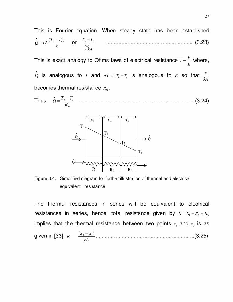
This is Fourier equation. When steady state has been established
x
TTkAQ ch )( −
=•
or
kAx
TT ch − …………………………………….………….. (3.23)
This is exact analogy to Ohms laws of electrical resistance R
EI = where,
•
Q is analogous to I and =∆T ch TT − is analogous to E so that kA
x
becomes thermal resistance thR .
Thus th
ch
R
TTQ
−=
•
………………………………………………………….………(3.24)
Figure 3.4: Simplified diagram for further illustration of thermal and electrical
equivalent resistance
The thermal resistances in series will be equivalent to electrical
resistances in series, hence, total resistance given by 321 RRRR ++=
implies that the thermal resistance between two points 1x and 2 x is as
given in [33]: =R kA
xx )( 12 −……………………………………………….……….(3.25)
•
Q
•
Q
•
Q
Th
T1
T2
Tc
R1 R2 R3
x2 x1 x3

28
CHAPTER FOUR
THERMAL MODEL DEVELOPMENT AND PARAMETER COMPUTATION
4.1 CYLINDRICAL COMPONENT AND HEAT TRANSFER ANALYSIS The heat transfer processes is summarized in the simplified diagram of
induction motor shown in figure (4.1) below. Conduction also occurs in the
air-gap, between stator slots and stator iron and between rotor bars and
rotor iron.
4.2 CONDUCTIVE HEAT TRANSFER ANALYSIS IN INDUCTION MOTOR
The rotor, stator, shaft and some other parts of the induction motor are
analyzed on the basis of the general cylindrical component as shown in
figure (4.2) below.
Ambient (convection and radiation)
Figure 4.1: Heat transfer mechanism in squirrel cage induction machine
Rotating stator flux
Stator (conduction)
3-Phase Supply
Rotor (conduction)
T3
T1
T2
T4
r1
L
r2

29
Figure 4.2: General cylindrical component
T1 ,T2 and T3 , T4 represent the inner and the outer surface temperatures of
the components while r2 and r1 denote the inner and the outer radius
respectively. In the same way, if one end of the cylinder is cut out, it will
give rise to a ring or what is referred to as annulus ring as shown in figure
(4.3).
In arriving at the expression for the thermal resistance networks in line
with the conduction of heat across the general component, the following
assumptions are made:
i The heat flows are of axial and radial type and are independent.
ii A unique mean temperature represents the heat flows in both
directions.
iii Circumferential heat flow is not present.
iv The thermal capacity and heat generation are uniformly distributed.
r1
r2
Figure 4.3: Conductive Thermal circuit- An annulus ring
T1
T2
T3
T4
L

30
In [45], the surfaces in the air-gap were further considered to be smooth
so that they can make use of the experimental results of Ball et al in [66].
According to [11], on adoption of those assumptions listed above, the
solution of the heat conduction equations in each of the axial and radial
directions yields two separate three-terminal network as shown in figure
(4.4) below.
Figure 4.4: Three terminal networks of the axial and radial networks In the above figure, 1T and 2T , 3T and 4T represent the surface
temperature of components, and the third, the mean or average
temperature mT of the component at which any internal heat generation u
or thermal storage thC is introduced. The central node of each network is
to give the mean temperature of the component but for the internal heat
generation or storage. The values of the thermal resistance according to
[67] and also in [14] come directly from the independent solutions of the
heat conduction equation in the axial and radial directions. These are
obtained considering the physical and cylindrical dimensions cum the
3T
u,Cth
2T
4T
1T
R2r
R1a
R2a
mT
R1r
R3a R3r
31
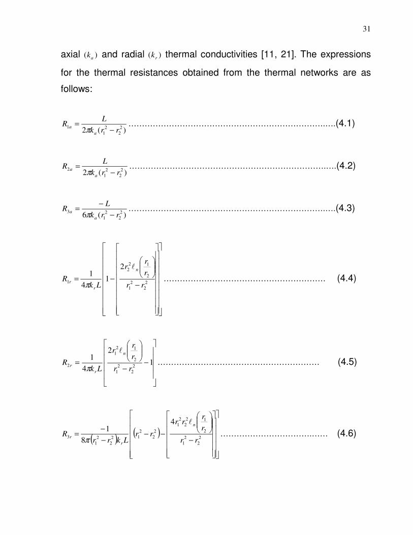
axial )( ak and radial )( rk thermal conductivities [11, 21]. The expressions
for the thermal resistances obtained from the thermal networks are as
follows:
)(2 2
2
2
1
1rrk
LR
a
a−
=π
……………………………………………………………….….(4.1)
)(2 2
2
2
1
2rrk
LR
a
a−
=π
……………………………………………………………….….(4.2)
)(6 2
2
2
1
3rrk
LR
a
a−
−=
π……………………………………………………………….….(4.3)
−
−=2
2
2
1
2
12
2
1
2
14
1
rr
r
rr
LkR
n
r
r
l
π…………………………………………………… (4.4)
−−
= 1
2
4
12
2
2
1
2
12
1
2rr
r
rr
LkR
n
r
r
l
π…………………………………………………… (4.5)
( )( )
−
−−−
−=
2
2
2
1
2
12
2
2
1
2
2
2
12
2
2
1
3
4
8
1
rr
r
rrr
rrLkrr
R
n
r
r
l
π…………………………….…… (4.6)

32
The total thermal capacitance of the cylinder is determined from the
density of the material ρ , the specific heat capacity pC and the motor
dimensions as follows:
( )LrrCC pth
2
2
2
1 −= πρ ………………………….………………………………………….(4.7)
The variation in the internal energy of the machine components with time
will be accounted for by the transient analysis hence the introduction of
the thermal capacitance.
......................................................................................................PPolth MCCVC == ρ ….(4.8)
where
M is mass and olV is volume
The networks of figure (4.4) are in one-dimension and can be combined
by connecting the two points of mean temperature ( aR3 and rR3 ) together.
The thermal network can be reduced to a much simpler one as in figure
(4.5) if we assume a symmetrically distributed temperature in the cylinder
about the central radial plane such that the temperature 3T and 4T on the
faces of the cylinder are equal. This will warrant that the modelling of half
of the cylinder be carried out with half of the heat generation and thermal
capacitance considered. This will appreciably reduce figure (4.4) to figure
(4.5) as shown below.
1θ
2θ
u, C
mθ
Ra
Rc
43 θθ =
Rb
Rm
1T
2T
u, Cth
mT
Ra
Rc
43 TT =
Rb
Rm

33
Figure 4.5: The combination of the axial and radial networks for a symmetrically distributed temperature about the central radial plane.
A close observation of figure (4.5) reveals four thermal resistances;
cba RRR ,, and mR lumped together to two internal nodes. The thermal
resistances are now given as:
( )2
2
2
1
316
2rrk
LRRR
a
aaa−
=+=π
………………………..………………………..….……(4.9)
−
−==2
2
2
1
2
12
2
1
2
12
12
rr
r
rr
LkRR
n
r
rb
l
π………………………………………………..…(4.10)
−−
== 1
2
2
12
2
2
2
1
2
12
1
2rr
r
rr
LkRR
n
r
rc
l
π…………………………………………………..…. (4.11)
( )( )
−
−+−
−==
2
2
2
1
2
12
2
2
1
2
2
2
12
2
2
1
3
4
4
12
rr
r
rrr
rrLkrr
RR
n
r
rm
l
π…………………………..… (4.12)
The model of figure (4.5) can be adapted for different thermal
conductivities in both directions which makes for easy consideration of the
thermal effects of the stator and the rotor laminations.
The general cylinder models the solid rod, say the shaft of induction motor
if the expressions given above as the radius 2r , tends to zero and the
node corresponding to the central temperature 2T is removed.

34
4.3 CONVECTIVE HEAT TRANSFER ANALYSIS IN INDUCTION MOTOR
Thermal resistance value given by cR , models the convective heat
transfer between open parts of the solid materials and the cooling air both
inside and outside. As stated earlier it has the value
11 −−= ccc AhR ……………………………………………………… ……...…….………(4.13)
Where =ch boundary film coefficient (convective heat transfer coefficient)
and =cA surface area in contact with the cooling air.
Film coefficients normally used in the study of convective heat transfer in
induction motor according to [11] are four in number namely: between
(a) frame and external air
(b) stator or rotor and air-gap
(c) stator iron, rotor, end-windings or end-cap and end-cap air
(d) rotor cooling holes and circulating end-cap air.
It further stated that for a given surface, a film coefficient applies when the
machine is stationary, that is, the external and internal fans are not
functional; a second film coefficient applies when the machine is rotating.
Hence, the film coefficient for the stages (a) – (d) can be denoted by
, ; aras hh , ; brbs hh crcs hh ; and drds hh ; respectively. The work hinted that
coefficients due to case ‘a’ above can be found directly from test if the
motor is run at constant load until thermal equilibrium is reached, arh is
then determined from the surface ambient temperature gradient and the

35
total machine loss, the ash being similarly found from a low voltage locked
rotor test, where under thermal equilibrium, the heat dissipated from the
motor surface is equal to the total electric power input. The rest of film
coefficients were obtained through various means as described in [68-71].
Concerning the air-gap, the two main parts, the rotor and the stator are in
the likes of two concentric cylinders in relative rotatory motion to each
other. Aside from the large induction motor types any heat emitted from
the rotor surface moves unhindered and across the air-gap to the stator.
The axial heat flow, if any, from the air gap to the adjoining endcap air is
very negligible, and is not given regard. The film coefficients of the air-gap
1h , in terms of a dimensionless Nusselt number uN , the air-gap width agwL
and thermal conductivity of air cT is related thus:
agw
airu
L
kNh =1 …………………………………….……………………………………(4.14)
The value of the Nusselt number for the convective heat transfer between
two smooth cylinders in rotatory motion is given in [71]. However, there is
greater heat transfer across the air-gap than achieved by the smooth
cylinder equations. This is due to the effect of additional fluid disturbances
carried by the winding slots. According to Gazley [69], his experimental
results show that about ten percent (10%) increase in heat transfer is as a
result of the slot effects.
4.4 DESCRIPTION OF MODEL COMPONENTS AND ASSUMPTIONS The construction of the induction machine under study is as presented in
figures (4.20) and (4.21) below with the parts labeled as indicated. A

36
better understanding of the modeling follows from these few descriptions
given below on some of the parts.
1. Ambient Air 6. Fan 11. Rotor iron
2. Rotor winding 7. End winding 12. Cooling rib
3. Stator iron 8. Bearing 13. Stator teeth
4. Air gap 9. Endring 14. Frame
5. Stator winding 10. Shaft
Figure 4.6: Squirrel Cage Induction Machine Construction
1
2
3
4
5
6
7
8
9
10
11
13
12
1
2
8
13
4
6
7
12
14
11
. .
5
8
9
10
3

37
FRAME: This is an embodiment of the entire ribbed cooling structure and
the endcaps. The frame absorbs heat from the stator across the frame-
core contact resistance, it also absorbs heat from the endcap air by
convection. The modelling elements of the frame are different because
the frame is thicker at the ends. The entire frame is considered to be at
uniform temperature and can dissipate heat externally via single frame to
ambient convective thermal resistance. The thermal resistance between
two frame elements is thus:
1)2( −+= ArbLR cc λπλ where A is cross sectional area of the cooling fins, b
is the thickness of frame, r is the mean radius of the frame, L is the
length of frame and cλ is the conductivity.
STATOR IRON: This is made up of the stator lamination pack.
The teeth are not included here. This is modeled using the general form
which is modified to take care of anisotropy due to the laminations. This is
handled by the introduction of a stacking factor in the radial direction and
by the use of a value lower than that of mild steel for the axial conductivity
obtained from [68]. The stator yoke elements are considered as hollow
cylinders with thermal resistance in the radial direction given by:
1
21 )2)( ( −−= LkrnrnR cπll where 1 r and 2 r are the outer and inner radii of the
cylinder.
1. End-winding cooling duct 6. Stator teeth 11. Rotor end
2. Frame 7. Stator winding 12. Shaft
3. Radial cooling duct 8. Air-gap 13. End-winding space(lower)
4. End-winding space(upper) 9. Rotor core
5. Stator yoke 10. Rotor teeth
Figure 4.7: The geometry of High Speed Induction Machine
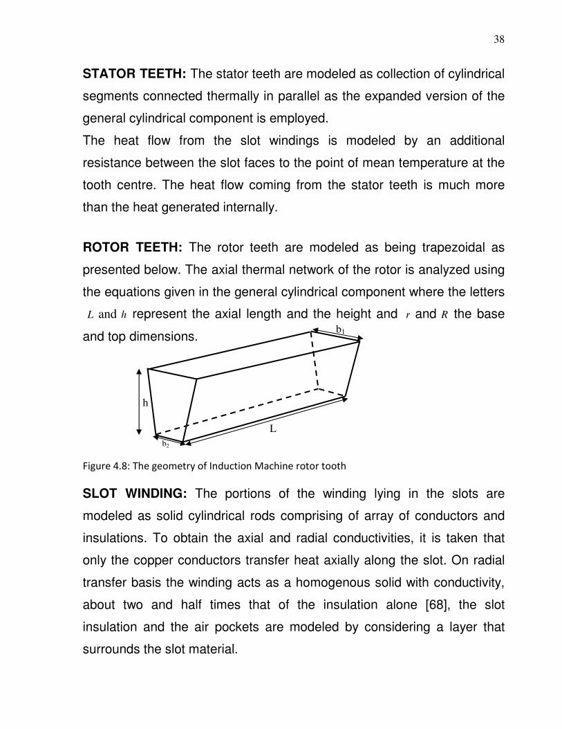
38
STATOR TEETH: The stator teeth are modeled as collection of cylindrical
segments connected thermally in parallel as the expanded version of the
general cylindrical component is employed.
The heat flow from the slot windings is modeled by an additional
resistance between the slot faces to the point of mean temperature at the
tooth centre. The heat flow coming from the stator teeth is much more
than the heat generated internally.
ROTOR TEETH: The rotor teeth are modeled as being trapezoidal as
presented below. The axial thermal network of the rotor is analyzed using
the equations given in the general cylindrical component where the letters
L and h represent the axial length and the height and r and R the base
and top dimensions.
Figure 4.8: The geometry of Induction Machine rotor tooth
SLOT WINDING: The portions of the winding lying in the slots are
modeled as solid cylindrical rods comprising of array of conductors and
insulations. To obtain the axial and radial conductivities, it is taken that
only the copper conductors transfer heat axially along the slot. On radial
transfer basis the winding acts as a homogenous solid with conductivity,
about two and half times that of the insulation alone [68], the slot
insulation and the air pockets are modeled by considering a layer that
surrounds the slot material.
b1
L
b2
h

39
ENDWINDING: This is modeled as a uniform torroidal material depicting
the circumferential mesh of conductors and insulation, the legs are
considered as short cylindrical extensions of the stator slot windings. An
axial heat transfer is assumed to occur from the mean temperature point
in the torroid to the stator slot winding along the copper conductors of the
legs. The heat transfer from the end windings is usually due to convection
with little trace of radiation.
AIRGAP: The air gap forms a connection between the stator teeth, the
part of the stator winding exposed in the slot openings and the rotor
surface. The corresponding thermal resistances are found from the
contact areas of these solids and the air-gap film coefficient. The heat
flow in the air-gap is mainly by conduction and convection. Some
researchers [68, 69, 70] have investigated the heat flow in the air-gap
between concentric cylinders with the thermal effect considered in [71].
Laminar flow was associated with small motors at low speeds due to
absence of axial flow, there was however a drift to turbulent flow with
reasonable increase in speed. The turbulent mode is defined better using
the Taylor number [69] which can also be presented as
F
aN
g
Ta 2
32
ν
δω= ……………………………………………………………………………(4.15)
where ω = angular speed, ga = average air gap radius, δ = air gap
=2ν kinematic viscosity, 1≅F is a factor of geometry, TaN = Taylor number
For the case of small machine at low speed the heat transfer coefficient
becomes ch and is related to Nusselt number uN , as

40
δ2
cuc
kNh = ……………………………………………………………………………....(4.16)
From the above equation and with L as the axial length of the element,
thermal resistance between a rotor element and a stator teeth element is
determined as: .................................................................2
1
LhaR
cgπ= ……….(4.17)
ENDCAP AIR: The circulating air in the endcap is considered as having a
uniform temperature. A single film coefficient is preferred for the
description of its convective heat transfer.
ROTOR IRON: The rotor is made up of several thin steel laminations
with evenly spaced bars, which are made up of aluminum or copper,
along the periphery. In the most popular type of rotor (squirrel cage rotor),
these bars are connected at ends mechanically and electrically by the use
of rings. According to [72], more or less 90% of induction motors have
squirrel cage rotors. This is because the squirrel cage rotor has a simple
and rugged construction. The rotor consists of a cylindrical laminated core
with axially placed parallel slots for carrying the conductors. Each slot
carries a copper, aluminum or alloy bar. These rotor bars are permanently
short-circuited at both ends by means of the end rings, as shown in
Figure (4.21). This total assembly resembles the look of a squirrel cage,
which gives the rotor its name. The rotor slots are not exactly parallel to
the shaft. Instead, they are given a skew for two main reasons. The first
reason is to make the motor run quietly by reducing magnetic hum and to
decrease slot harmonics. The second reason is to help reduce the locking
tendency of the rotor. The rotor teeth tend to remain locked under the
stator teeth due to direct magnetic attraction between the two. This

41
happens when the number of stator teeth is equal to the number of rotor
teeth. The rotor is mounted on the shaft using bearings on each end; one
end of the shaft is normally kept longer than the other for driving the load.
Some motors may have an accessory shaft on the non-driving end for
mounting speed or position sensing devices. Between the stator and the
rotor, there exists an air gap, through which due to induction, the energy
is transferred from the stator to the rotor. The generated torque forces the
rotor and then the load to rotate. Regardless of the type of rotor used, the
principle employed for rotation remains the same.
As was considered for the stator iron, the laminations in the rotor iron are
handled in the same manner. The rotor elements are taken as having
thermal contact with the stator teeth. The thermal resistance between two
rotor elements is given as:
................................................................................................ANk
LR
bc
= ……..………(4.18)
where A = cross sectional area of a bar, L = distance between adjacent rotor elements
ck = conductivity of the bar material, bN = number of bars
1. End Ring 3. Conductors 5. Shaft
2. Bearing 4. Skewed Slots
Figure 4.9: Squirrel Cage Rotor
1
2
3
4
5

42
SHAFT: The shaft is modeled as a cylindrical rod with no internal heat
generation. The axial heat conduction is modeled as three sections. A
good thermal contact is assumed to exist between the shaft and the frame
across the bearings. Any shaft external to the bearing is therefore
considered to act as part of the frame. Thermal resistance between a
rotor element and a shaft element includes that due to the thermal
resistance via the rotor core which is given by:
Lk
r
rn
Rc
a
b
π2
=
l
..................................................................................... …..………………..(4.19)
where ar = radius of the shaft , ck = conductivity of the core material
L = distance between adjacent elements and br = radius of the bottom of rotor slots.
In light of the descriptions given so far on the machine, an equivalent
circuit representing some core parts is given in the figure below. Table
4.1 showing some geometric values and dimensions for the machine
parts is also presented.
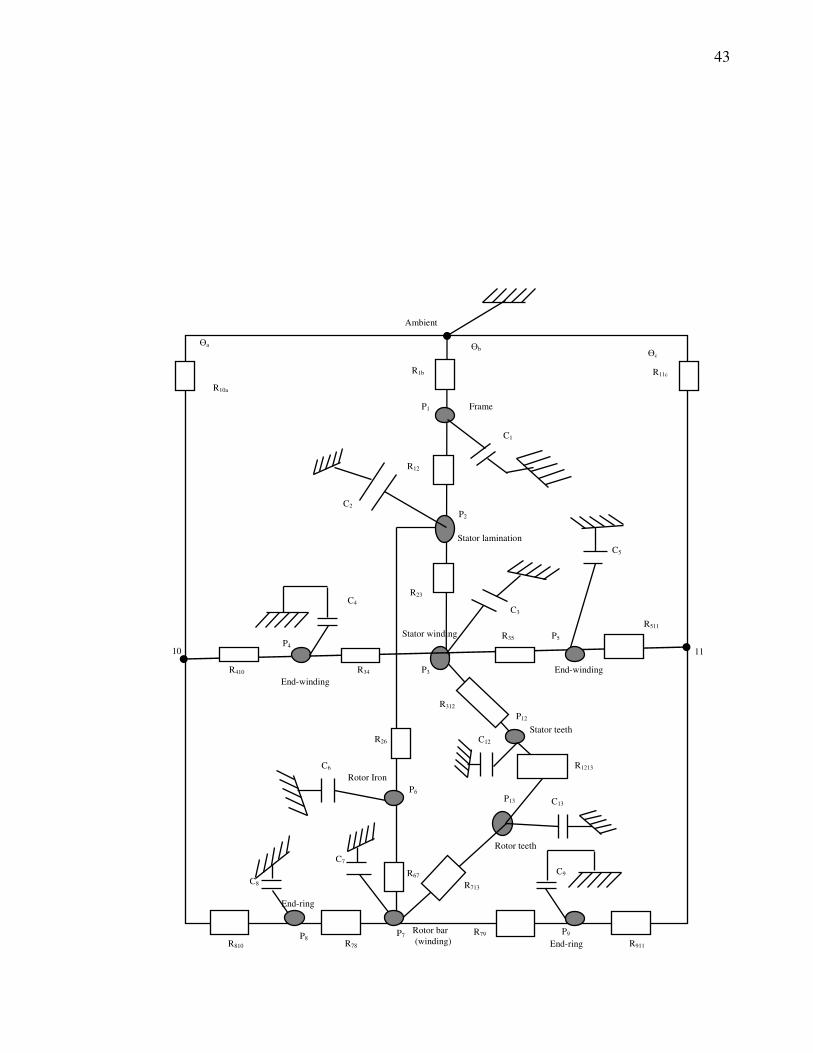
43
11
C4
C2
C1
R35 P5
R810
R511
End-ring
P8
R10a
Өc
P12
R312
R1213
C12 Stator teeth
P13
Rotor teeth
C13
R713
R79
Rotor Iron
Rotor bar
(winding)
End-ring
End-winding
End-winding
Frame
Stator lamination
Stator winding
Ambient
P1
R12
P2
Өa
R11c
Өb
R1b
R23
P3
P4 10
C8
C5
C3
P6
R67
P7
R78
R911
P9
C6
R26
R34 R410
C7
C9
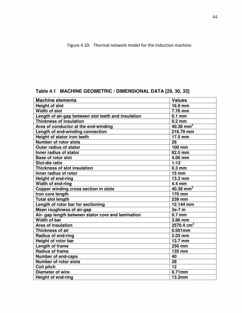
44
Table 4.1 MACHINE GEOMETRIC / DIMENSIONAL DATA [29, 30, 33]
Machine elements Values Height of slot 16.9 mm Width of slot 7.76 mm Length of air-gap between slot teeth and insulation 0.1 mm Thickness of insulation 0.2 mm Area of conductor at the end-winding 40.38 mm2 Length of end-winding connection 216.79 mm Height of stator iron teeth 17.5 mm Number of rotor slots 28 Outer radius of stator 100 mm Inner radius of stator 62.5 mm Base of rotor slot 4.06 mm Slot-die ratio 1:12 Thickness of slot insulation 0.3 mm Inner radius of rotor 15 mm Height of end-ring 13.2 mm Width of end-ring 4.4 mm Copper winding cross section in slots 40.38 mm2 Iron core length 170 mm Total slot length 239 mm Length of rotor bar for sectioning 12.144 mm Mean roughness of air-gap 3e-7 m Air- gap length between stator core and lamination 0.7 mm Width of bar 3.86 mm Area of insulation 2570.4 cm2 Thickness of air 0.001mm Radius of end-ring 2.03 mm Height of rotor bar 13.7 mm Length of frame 250 mm Radius of frame 135 mm Number of end-caps 40 Number of rotor slots 28 Coil pitch 12 Diameter of wire 0.71mm Height of end-ring 13.2mm
Figure 4.10: Thermal network model for the Induction machine
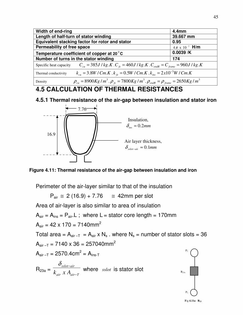
45
4.5 CALCULATION OF THERMAL RESISTANCES
4.5.1 Thermal resistance of the air-gap between insulation and stator iron
Perimeter of the air-layer similar to that of the insulation
Pair ≅ 2 (16.9) + 7.76 ≅ 42mm per slot
Area of air-layer is also similar to area of insulation
Aair = Ains = Pair.L ; where L = stator core length = 170mm
Aair = 42 x 170 = 7140mm2
Total area = Aair –T = Aair x Ns . where Ns = number of stator slots = 36
Aair –T = 7140 x 36 = 257040mm2
Aair –T = 2570.4cm2 = Ains-T
R23a = Tairair
airsslot
Axk −
−
δ where sslot is stator slot
Width of end-ring 4.4mm Length of half-turn of stator winding 39.667 mm Equivalent stacking factor for rotor and stator 0.95 Permeability of free space -710 x 4π H/m
Temperature coefficient of copper at 200C 0.0039 /K
Number of turns in the stator winding 174
Specific heat capacity KkgJCcu ./385= , KkgJC fe ./460= , KkgJCC frameendR ./960==
Thermal conductivity KCmWkcu ./8.3= , KCmWk fe ./5.0= , KCmWxkins ./102 3−=
Density 3/8900 mKgcu =ρ ,
3/7800 mKgfe =ρ ,3/2650 mKgframeendR == ρρ
7.76
Insulation,
mmins 2.0=δ
16.9
Air layer thickness,
mmairsslot 1.0≈−δ
Figure 4.11: Thermal resistance of the air-gap between insulation and iron
P2
R23a
P3
Fig 4.11a R23

46
airk = 0.28 x 10⁻³ W/cm.K = thermal conductivity of air
R23a = 4.2570 1028.0
01.03
xx− hence R23a = 13.9x10⁻³ K/W
For half of the machine, we have,
R23a.half = 27.8 x10⁻³ K/W
4.5.2 The thermal resistance of the insulation slot, R23b
R23b = Tinsins
ins
Ak −x
δ , insk = 2x10⁻³ W/cm.K
R23b = 4.2570x 10²
02.03−
x
R23b = 3.89 x 10⁻³ K/W
For half of the machine
R23b.half = 7.78 x 10⁻³ K/W
Therefore, the thermal resistance between the stator winding and stator
iron becomes,
R23 = R23a + R23b
R23= 13.9 x 10⁻³ + 3.89 x 10⁻³
R23 = 17.79 x 10⁻³K/W
For half of the machine,
R23 = 35.58 x 10⁻³K/W
P2
R23b
P3
Fig 4.11b R23

47
4.5.3 Thermal resistance between the stator iron and the yoke, R12
Stator outside radius, ro = 100mm
Stator inside radius, ri = 62.5mm
Stator core length, L = 170mm
fek = 0.5 W/cm.K = thermal conductivity of iron
hy = ro – (17.5 + ri) = height of yoke
5mm
ro
Ry
Figure 4.12: Thermal resistance between the stator iron and the yoke, R12
hy
ri
17.5

48
hy = 100 – 62.5 – 17.5, hy = 20mm
Radius of yoke = Ry
Ry = ro -2
yh = 100-10
Ry = 90mm
∴R12a = yfe
y
Ak
h
Ay = Area of the yoke
Ay = 2π RyL Kfe (where Kfe is iron stacking factor)
Ay = 2π x 90 x 170 x 0.95 = 91326.1mm2
Ay = 913.26cm2
R12a = 26.913 x 5.0
2
R12a = 4.38 x 10⁻³ K/W
For half of the machine
R12a.half = 8.76 x 10⁻³ K/W
4.5.4 Thermal resistance of the air-layer between insulation and yoke, R12b
R12b = yokeairair
airyoke
Ak −
−δ
δ yoke-air = 0.01mm
airk = 0.28 x 10⁻³ W/cm.K
ro = outside stator radius = 100mm
Ls = stator core length = 170mm
Aair – yoke = 2π ro Ls
= 2π x 100 x 170
= 1068.14cm2
R12a
P2
Fig 4.12a R12
R12b
P2
Fig 4.12b R12

49
R12b = 14.1068 x 10x28.0
001.03−
R12b = 3.34x10⁻³ K/W
For half of the machine, R12b.half = 6.68 x10⁻³K/W
R12 = R12b + R12a = 3.34x10⁻³ + 4.38 x 10⁻³
R12 = 7.72 x 10⁻³ K/W
For half of the machine,
R12 = 0.01544 K/W = 15.44 x 10⁻³K/W
4.5.5 Thermal resistance between stator iron and end- winding, R34
Considering a slot and half of the machine, we have,
R34 – slot = ccu
ew
Ak
LL
x
44+
Conductor area = Ac = 40.38 mm2 = 0.4038 cm2
L/2 Endwinding
Figure 4.13: Thermal resistance between the stator iron and the end-winding, R34
L/4
L
L/4
L/4
Endwinding
P3
P4
R34
Fig. 4.13a
R34 =R35

50
Length of end winding = ewL
ewL = 216.79 mm
cuk ≅ 3.8 W/cm.K = the thermal conductivity of copper
L = 170 mm
R35-slot = 4038.0 x 8.3
4
7.21
4
17+
= 6.305 K/W
Considering the entire slots, we have
R35 = s
slot
N
R −35 = 36
305.6
R35 = 0.1751 K/W
For the whole machine, we have
R35 = 2
1751.0 = 0.08755 K/W
4.5.6 Thermal resistance between Rotor Bar and the end ring, R67
L
2
LLbar −
∆ L1
∆ L
∆ L2

51
Nr = 28 is Number of rotor slots
L = 170 mm is the stator iron core length
slotL = 239 mm is the entire slot length
cuk = 3.8 W/cm.K
∆ L 1 = 4
170
4=
L = 42.5 mm
∆ L 2 =
−
2
170240x
2
1 = 17.5 mm
∆ L = ∆ L 1 + ∆ L 2 = 60mm
Arbar = hrbar x brbar
hrbar = 13.17mm
brbar = 4.06 mm
Arbar = 13.17 x 4.06 = 53.47 mm2
For one rotor bar, R67’ becomes,
R67’ = rbarcu Ak
L∆
R67’ = 5347.0 x 8.3
6
R67’ = 2.953 K/W
∴The thermal resistance for all the rotor bars with the half of the
machine considered, gives
Lendr
Figure 4.14: Thermal resistance between Rotor Bar and the end ring, R67
P7
R67
P6
Fig 4.14a
R67

52
R67 = R67’xrN
1
R67 = 2.953 x 28
1
R67 = 0.1055 K/W
For the whole machine, we have
R67 = 2
1055.0 = 0.05275 K/W
R67 = 0.05275 K/W
4.5.7 Thermal resistances of the rotor bar
Acu = 2
L brslot =
2
17x 4.06 x 10-1 = 3.451 cm2
with a base of 35mm
R45rb = 451.3x 8.3
350.0= 26.76 x 10⁻³ K/W (since cuk =3.8 W/cm.K)
For all the rotor slots, Nr = 28, hence R45=28
1 x R45rb
R45 = 28
1 x 26.76 x 10-3 K/W
R45 = 0.956 x 10⁻³ K/W
4.5.8 Thermal resistances from the Rotor slot to end ring, R78
brslot = 4.06 mm
cuk =3.8 W/cm.K
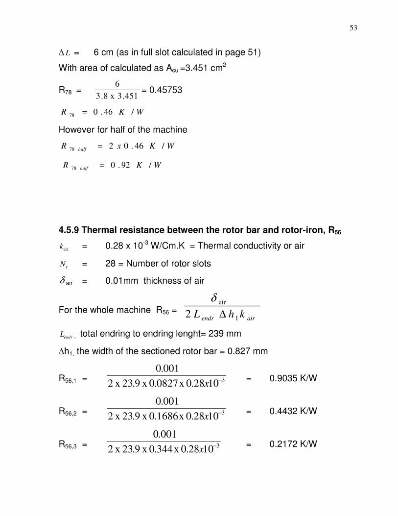
53
∆ L = 6 cm (as in full slot calculated in page 51)
With area of calculated as Acu =3.451 cm2
R78 = 451.3x 8.3
6= 0.45753
WKR /46.078 =
However for half of the machine
WKxR half /46.0278 =
WKR half /92.078 =
4.5.9 Thermal resistance between the rotor bar and rotor-iron, R56
airk = 0.28 x 10⁻³ W/Cm.K = Thermal conductivity or air
rN = 28 = Number of rotor slots
δ air = 0.01mm thickness of air
For the whole machine R56 = airendr khL 1
air
2
∆
δ
endrL , total endring to endring lenght= 239 mm
∆h1, the width of the sectioned rotor bar = 0.827 mm
R56,1 = 31028.0 x 0827.0 x 9.23 x 2
001.0−
x = 0.9035 K/W
R56,2 = 31028.0 x 1686.0 x 9.23 x 2
001.0−
x = 0.4432 K/W
R56,3 = 31028.0 x 344.0 x 9.23 x 2
001.0−
x = 0.2172 K/W

54
R56,4 = 31028.0 x 6191.0 x 9.23 x 2
001.0−
x = 0.1207 K/W
R56,5 = R56,1 = 0.9035 K/W
∴ 5,564,563,562,561,5656
111111
RRRRRR++++=
9035.0
1
1207.0
1
2172.0
1
4432.0
1
9035.0
11
56
++++=R
= ( )9035.0x 1207.0x 2172.0x 4432.0x 9035.0
010497.00785807.00436680.00214005.00104977.0 ++++
3
56 10484690.9
1646446.01−
=xR
; R56 = 1646446.0
10484690.9 3−x
= 0.05761 K/W
For half of the machine we have,
R56,1.half = 1.807 K/W , R56,2.half = 0.8864 K/W
R56,3.half = 0.4344 K/W , R56,4.half = 0.2414 K/W
R56,5.half = 1.807 K/W , R56.half = 0.11522 K/W
The number of rotor slots 28r =N , therefore
For all the slots, and for the whole machine
R56,1 = rN
R56,1
= 28
0.9035 = 0.03227 K/W
R56,2 = 0.01583 K/W , R56,3 = 7.757 x 10⁻³ K/W
R56,4 = 4.3107 x 10⁻³ , R56,5 = 0.03227 K/W
∴ R56 = 2.0575 x 10⁻³ K/W
For half of the machine, we have
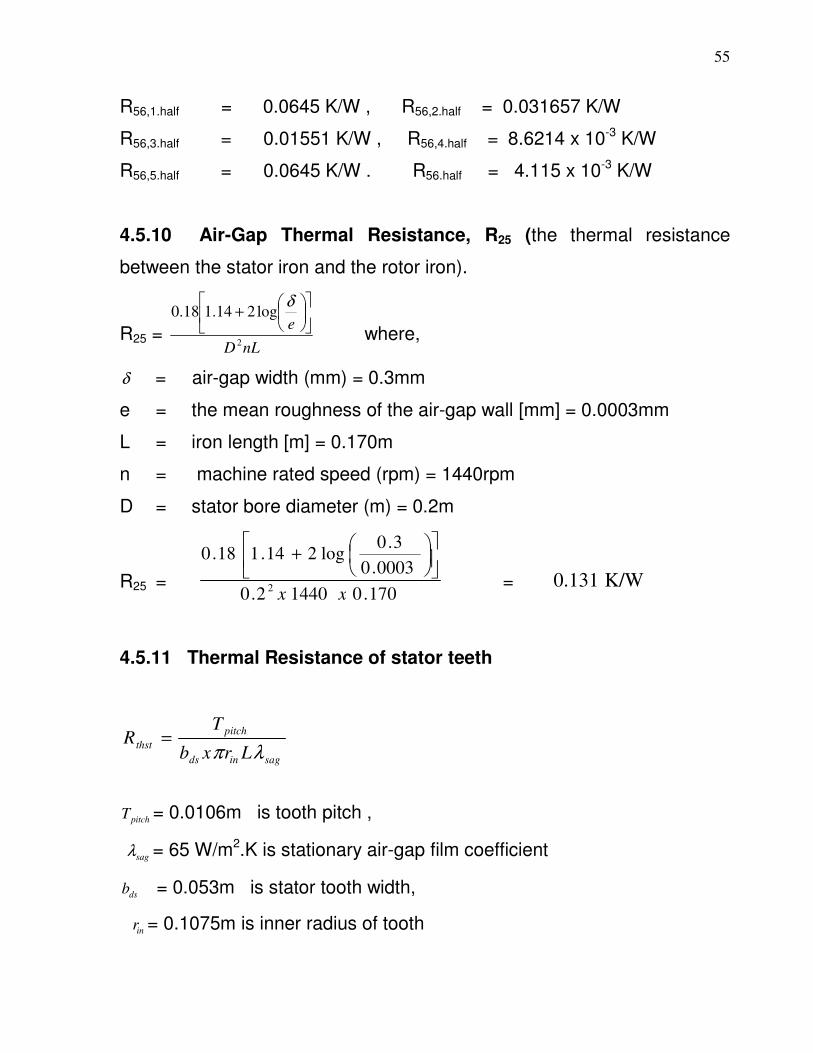
55
R56,1.half = 0.0645 K/W , R56,2.half = 0.031657 K/W
R56,3.half = 0.01551 K/W , R56,4.half = 8.6214 x 10⁻³ K/W
R56,5.half = 0.0645 K/W . R56.half = 4.115 x 10⁻³ K/W
4.5.10 Air-Gap Thermal Resistance, R25 (the thermal resistance
between the stator iron and the rotor iron).
R25 = nLD
e2
log214.118.0
+
δ
where,
δ = air-gap width (mm) = 0.3mm
e = the mean roughness of the air-gap wall [mm] = 0.0003mm
L = iron length [m] = 0.170m
n = machine rated speed (rpm) = 1440rpm
D = stator bore diameter (m) = 0.2m
R25 = 170.0 1440 2.0
0003.0
3.0log214.1 18.0
2xx
+
= K/W0.131
4.5.11 Thermal Resistance of stator teeth
pitchT = 0.0106m is tooth pitch ,
sagλ = 65 W/m2.K is stationary air-gap film coefficient
dsb = 0.053m is stator tooth width,
inr = 0.1075m is inner radius of tooth
saginds
pitch
thstLrxb
TR
λπ=
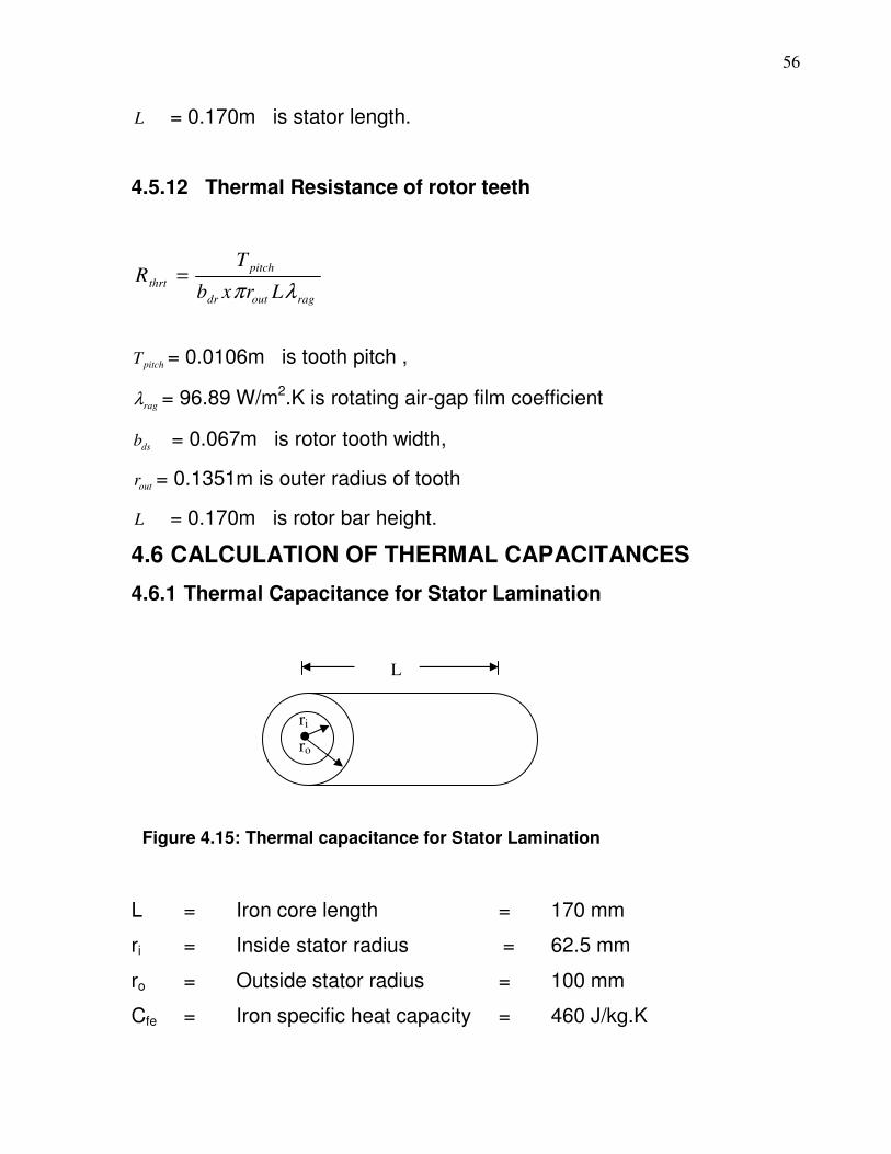
56
L = 0.170m is stator length.
4.5.12 Thermal Resistance of rotor teeth
pitchT = 0.0106m is tooth pitch ,
ragλ = 96.89 W/m2.K is rotating air-gap film coefficient
dsb = 0.067m is rotor tooth width,
outr = 0.1351m is outer radius of tooth
L = 0.170m is rotor bar height.
4.6 CALCULATION OF THERMAL CAPACITANCES
4.6.1 Thermal Capacitance for Stator Lamination
L = Iron core length = 170 mm
ri = Inside stator radius = 62.5 mm
ro = Outside stator radius = 100 mm
Cfe = Iron specific heat capacity = 460 J/kg.K
ro
L
ri
Figure 4.15: Thermal capacitance for Stator Lamination
ragoutdr
pitch
thrtLrxb
TR
λπ=

57
Kfe = Lamination stacking factor = 0.95
feρ = Lamination iron density = 7800kg/m3
CTotal = feρ Cfe V
V = π )r - (r 2
i
2
o Kfe L
V = (0.12 – 0.06252) π x 0.95 x 0.170
V = 3.092 x 10⁻³ m3
∴ CTotal = 7800 x 460 x 3.092 x 10-3
CTotal = 11094 J/K (for the whole lamination)
CTotal.half = 5547 J/K (for half of the lamination)
4.6.2 Thermal Capacitance for Stator Iron
Area of the stator slot = slotA
slotA = 2
5.42) (7.76 + x 14.2 +
2
x2.712 π
17.5
ri = 62.5
7.76
14.2 16.9
5.42
0.6
2.71
Figure 4.16: Thermal capacitance for stator iron
C2
P2

58
= 93.578 + 11.536
slotA = 105.114 mm2
Total volume of slot, slotTV
slotTV = Ns x slotA x Ls
Ns = total number of stator slots = 36
L = iron core length = 170 mm
slotTV = 36 x 105.114 x 10-6 x 0.170
= 6.433 x10⁻⁴ m3
∴ Stator slot thermal capacitance, thslotC is
thslotC = Kfe slotTV CL Lρ
thslotC = 0.95 x 6.433 x 10-4 x 7800 x 460
thslotC = 2192.75 J/K
∴ The thermal capacitance of the stator lamination, CthsLam is
CthsLam = CT - thslotC
CthsLam = 11094 – 2192.75
CthsLam = 8901.25 J/K = C2
If half of the machine is considered, Cthslam becomes
Cthslam.half = 4450.625 J/K
4.6.3 Thermal Capacitance for Stator Windings, C3
C3 = cuC cuρ cuA x Ls x Ns
cuC = Copper specific heat (385 J/kg.k)
cuρ = Copper density (8900 kg/m3)
Stator winding
C3

59
cuA = Copper winding cross section in slots (40.38 mm2)
Ns = Number of stator slots (36)
L = Stator length (170 mm)
D = Wire diameter (0.71 mm)
C3 = 385 x 8900 x 40.38 x 10-6 x 0.170 x 36
C3 = 846.776 J/K
For half of the machine, C3.half = 423.388 J/K
4.6.4 Thermal Capacitance for End Windings, C4
L = 170 mm
L = 170 mm
Lm
(a)

60
L = Stator core length
Lm = Mean length of the end winding
Slot die = 1: 12
Number of stator slots, Ns = 36
Lm = 2π avslotr x36
11
avslotr = stator inside radius ( ir ) + the 2
height slot
= +5.62 2
5.17
Lm = 2π x 71.25 x 36
11
Lm = 136.79 mm; then the total length = Lst
Lst = Lm + 2 x 40
Lst = 136.79 + 80
Lst = 216.79 mm
∴Average conductor length = Lst + L
= 216.79 + 170
= 386.79 mm
1 12
40 mm
Lm
Figure 4.17 a,b,c: Thermal capacitances for end winding
(b)
(c)
C4
P4
Fig.4.17d
C4

61
Total winding length (Lmt) = 2 (Lst + L)
Lmt = 773.58 mm
C4 = cuC cuρ cuA x Lst x Ns
C4 = 385 x 8900 x 40.38 x 10-6 x 216.79 x10-3 x 36
C4 = 1079.84 J/K
Half of the machine, C4.half = 539.92 J/K
4.6.5. Rotor Iron Thermal Capacitance, C6
Shaft
End ring
239
170 RR
34.5
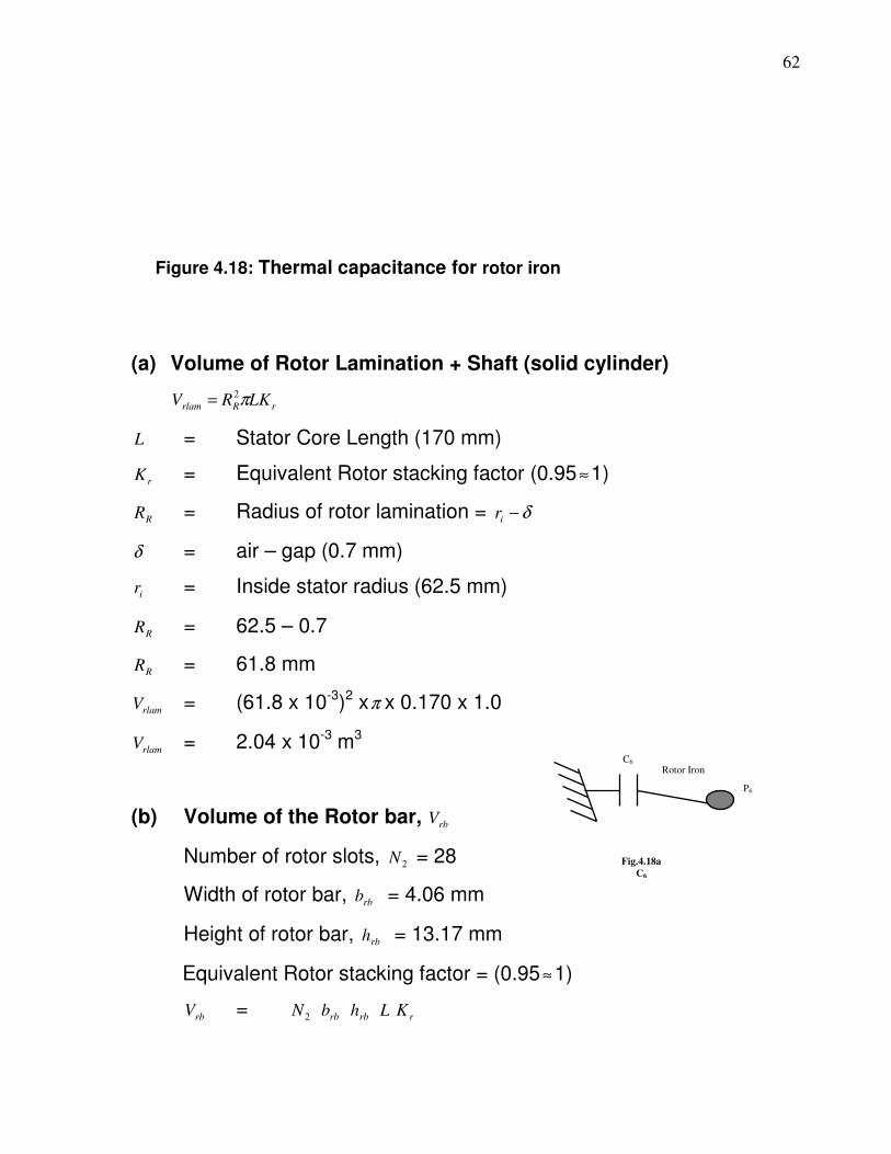
62
(a) Volume of Rotor Lamination + Shaft (solid cylinder)
rRrlam LKRV π2=
L = Stator Core Length (170 mm)
rK = Equivalent Rotor stacking factor (0.95≈1)
RR = Radius of rotor lamination = δ−ir
δ = air – gap (0.7 mm)
ir = Inside stator radius (62.5 mm)
RR = 62.5 – 0.7
RR = 61.8 mm
rlamV = (61.8 x 10⁻³)2 xπ x 0.170 x 1.0
rlamV = 2.04 x 10⁻³ m3
(b) Volume of the Rotor bar, rbV
Number of rotor slots, 2N = 28
Width of rotor bar, rbb = 4.06 mm
Height of rotor bar, rbh = 13.17 mm
Equivalent Rotor stacking factor = (0.95≈1)
rbV = 2N rbb rbh L rK
Figure 4.18: Thermal capacitance for rotor iron
Rotor Iron
P6
C6
Fig.4.18a
C6

63
rbV = 28 x 4.06 x 10-3 x 13.17 x 10-3 x 0.170 x 1
rbV = 2.545 x10⁻⁴ m3
(c) Total Volume, TV
TV = rlamV – rbV
TV = 2.04 x10⁻³ – 2.545 x 10⁻⁴
TV = 1.786 x 10⁻³ m3
(d) Rotor thermal capacitance, C6
C6 = TV FeFeCρ
Feρ = Iron density [7800 kg/m3]
FeC = Iron specific heat [460 J/kg.K]
C6 = 1.786 x 10-3 x 7800 x 460
C6 = 6408.17 J/K
For half of the machine,
C6.hallf = 3204.08 J/K
4.6.6. Rotor Bar Thermal Capacitance, C7
bSt
hrb
hSt
bL
hL
a
a

64
Lb = abrb 2− ; Lh = ahrb 2−
insδ = insulation thickness (0.1 mm)
rbb = 4.06 mm ; rbh = 13.17 mm
Lb = 3.86 mm ; Lh = 12.97 mm
Volume of the active part of the rotor bar, rbV
rbV = Lb Lh 2N L
= 3.86 x10-3 x 12.97 x 10-3 x 28 x1.0 x 0.17
rbV = 2.383 x 10⁻⁴ m3
rbarC = C7 = rbV CuCuCρ
C7 = 2.382 x 10-4 x 8900 x 385
C7 = 816.535 J/kg
Half of the machine, C7.half = 408.267 J/kg
4.6.7 Thermal Capacitance for Various Rotor- Bar Sections
Crb1
Crb2
Crb3
Crb4
0.827
1.686
3.44
6.191
0.827
brb
12.97 mm
Figure 4.19: Thermal capacitance for the Rotor bar
Crb5
C7
P7
Fig. 4.19a
C7

65
C7 = Crb1 + Crb2 +Crb3 + Crb4 + Crb5
∴ Crb1 + Crb2 +Crb3 + Crb4 + Crb5 ≡ 816.535
Crb1 = 97.12
827.0 x 816.535 = 52.06 J/kg
Crb2 = 97.12
686.1 x 816.535 = 106.14 J/kg
Crb3 = 97.12
44.3 x 816.535 = 216.57 J/kg
Crb4 = 97.12
191.6 x 816.535 = 389.76 J/kg
Crb5 = Crb1 = 52.06 J/kg
When half of the machine is considered we have,
Crb1.half = kgJ / 03.26 , Crb2.half = kgJ / 3.075 , Crb3.half = kgJ / 08.291 ,
Crb4.half = kgJ / 99.881 , Crb5.half = kgJ / 6.032 .
4.6.8 End Rings Thermal Capacitance, C8
4.06
RRing
13.17
hs
170
239
RRotor
dRing
Figure 4.20: Thermal Capacitance for the Various Rotor-Bar Sections

66
(i) Part of the slot outside the active part
Total slot length = 239 mm = LsL
Slot length outside the active part, La = LsL – L
La = 239 – 170
La = 69 mm
VsL = bL hL La . N2
= 3.86 x 12.97 x 69 x 28
VsL = 96724.03 mm3
= 9.672 x 10⁻⁵ m3
CsL = VsL cuρ cuC
= 9.672 x10-5 x 8900 x385
CsL = 331.41 J/K
(ii) The end- ring part
Area of the end-ring, Ar = rbb rbhx
Ar = 4.06 x13.17 mm
Ar = 53.47 x 10⁻⁶ m2
RR = Radius of rotor lamination = δ−ir
RRing = RR – hs – hrb - 2
Ringd
= 61.8 – 0.5 – 13.17 – 2
06.4
RRing = 46.10 mm
VRing = 2π RRing. Ar
Figure 4.21: Thermal capacitances for the End rings
End-ring
C8
P8
Fig.4.21a
C8

67
= 2π x 46.10 x 10-3 x 53.47 x 10-6
VRing = 1.549 x 10⁻⁵ m3
CRing = VRing cuρ cuC
1.549 x 10-5 x 8900 x 385
CRing = 53.08 J/K (for one ring)
CRingtotal = 106.16 J/K
Therefore the total thermal capacitance of the end-rings with the slot part
outside the active part included is
C8 = 331.41 + 106.16
C8 = 437.57 J/K
For half of the machine, C8.half = 218.785 J/K
4.6.9 Frame Thermal Capacitance, C1
C1 = Ce δe Vec + Cf δf Vf-e
δe = δf = 2650 kg/m3
Ce = Cf = 960 J/kg.K
(i) Vf-e = volume of frame without endcap
Vf-e = π 2
fr Kfe Lf
rf = ro + da
rf = 100 + 35 = 135 mm ; Lf = 250 mm
Vf-e=π x (0.135)2 x 0.25 x 0.95 m3 where,
Vf-e=13.6 x 10⁻³

68
ro = outside radius of the stator
Lf = length of the frame
Kfe = lamination stacking factor
da = distance between the stator winding and the frame
(ii) Vec = volume of end cap
Vec = ha wa La x ne x Kfe
ne = Number of end cap = 40
Vec = 23.66 x 10 -3 x 4.44 x 10-3 x 0.226 x 40 x 0.95
Vec = 9.02 x 10⁻⁴ m3
C1 = Cf δf Vf-e + Ce δe Vec
= 960 x 2650 x 13.6 x 10-3 + 960 x 2650 x 9.02 x 10-4
= 34598.4 + 2294.69C1 = 36893.09 J/K
For half of the machine, C1.half = 18446.55 J/K.
The calculated values of the thermal resistances and the thermal capacitances
used for the simulation are as shown in the table (4.2) below, other values
marked (*) are not calculated herein but are as given in [25, 28 and 31]:
TABLE 4.2: Calculated thermal capacitance and thermal resistance
values obtained from the thermal circuit.
Thermal Capacitances
Description of component location in the thermal circuit
SIM (J/kg)
LIM (J/kg)
C1 Frame thermal capacitance 18446.55 18446.55 C2 Thermal capacitance of stator lamination 4450.625 4450.625
C3 Thermal capacitance of stator winding 423.388 423.388 C4 End-windingR thermal capacitance 539.92 539.92 C5 Thermal capacitance of rotor iron 3204.08 3204.08 C6 Rotor bar thermal capacitance 408.267 408.267 C7 Thermal capacitance of end-ringR 218.785 218.785 *C8 Thermal capacitance of ambient air 1006 1006

69
C9 Thermal capacitance of end-ringL 218.785 C10 Thermal capacitance of ambient air 1006 C11 Thermal capacitance of end-windingL 539.92
*C12 Thermal capacitance of the stator teeth 341.33 *C13 Rotor teeth thermal capacitance 871.566 Thermal Resistances
(K/W)
(K/W)
*R1b between ambient and frame 0.0416 0.0416 R12 between frame and stator lamination 15.44e-3 15.44e-3 R23 between stator lamination and stator winding 35.58e-3 35.58e-3
R25 between stator lamination and rotor iron 0.131 0.131 R34 between stator winding and end-winding 0.1751 0.1751 *R48 of the end-winding 1.886 1.886 R56 between rotor bar (winding) and rotor iron 4.115e-3 4.115e-3 R67 between rotor bar and end-ring 0.1055 0.1055 R78 of the end-ring 0.932 0.932
R8c for ambient air 0.015 0.015 * R713 rotor bar and rotor teeth 0.002703 *R312 between stator teeth and stator winding 0.02245 *R1213 between stator teeth and rotor teeth 0.12576
CHAPTER FIVE
LOSSES IN INDUCTION MACHINE
5.1 DETERMINATION OF LOSSES IN INDUCTION MOTORS
Power losses that occur during the transfer of power from the electrical
supply to mechanical load give rise to the heating of the induction
machines. Some of the loss components were described in [72] under
iron losses, copper losses, harmonic losses, stray load losses and
mechanical losses.

70
There are five main losses that occur in an induction machine and these
are identified as follows:
1. Stator copper losses that occur as a result of the current flowing in the
stator.
2. Core losses linked to the magnetic flux in the machine, which is
independent of the load.
3. Stray load losses that vary with the driven load.
4. Rotor copper losses.
5. Friction and windage (rotational) losses that occur in the bearings
and ventilation ducts.
5.1.1 Stator and Rotor I2R Losses
These losses are major losses and typically account for 55% to 60% of
the total losses. I2R losses are heating losses resulting from current
passing through stator and rotor conductors. I2R losses are the function of
a conductor resistance, the square of current. This is one of the major
harmonic losses, a resistive loss of the rotor expressed as:
.......................................................................3 2
rrr RIP = ……………………………….…..(5.1)
where rI and rR are the current and resistance per phase respectively.
Resistance of conductor is a function of conductor material, length,
temperature and cross sectional area. The suitable selection of copper
conductor size will reduce the resistance. Reducing the motor current can
be accomplished by decreasing the magnetizing component of current.
This involves lowering the operating flux density and possible shortening
of air gap. Rotor I2R losses are a function of the rotor conductors (usually
aluminum) and the rotor slip. Utilization of copper conductors will reduce

71
the winding resistance. Motor operation closer to synchronous speed will
also reduce rotor I2R losses.
5.1.2 Core Losses
Core losses are those found in the stator-rotor magnetic steel and are due
to hysteresis effect and eddy current effect during 50 Hz magnetization of
the core material. These losses are independent of load and account for
20 – 25 % of the total losses [73]. The hysteresis losses which are a
function of the flux density are reduced by utilizing low loss grade of
silicon steel laminations. The reduction of flux density is achieved by
suitable increase in the core length of stator and rotor. Eddy current
losses are generated by circulating current within the core steel
laminations. These are reduced by using thinner laminations.
5.1.3 Friction and Windage Losses
Friction and windage losses result from bearing friction, windage and
circulating air through the motor [74-76] and account for 8 – 12 % of total
losses. These losses are independent of load.
5.1.4 Differential flux densities and Eddy-currents in the rotor bars
The rotor copper losses arise from the flux pulsations in the rotor teeth.
The differential flux densities of two adjacent rotor teeth will be an
indication of flux pulsation seen by a rotor bar. This occurs under no-load
which means that currents will flow in each bar.
The flux pulsations at no-load means eddy-currents and to prove this, the
rotor copper losses are in [77] calculated in a separate solution where the
rotor short circuit rings are neglected. The only loss that occurred was

72
that of the eddy currents. This shows that even under no-load the rotor
copper loss is significant and in this case the cause for overheating. In
[78], the eddy current losses of stator esP and rotor erP are calculated
using these formulae:
( ).................................................................................*5.1
22
s
dsqs
esR
VVP
+= …………….…. (5.5)
( ).....................................................................................*5.1
22
r
drqr
erR
VVP
+= …………….. (5.6)
while the copper losses at stator side cusP and at rotor side curP are
computed using the conventional formulae below.
( ) ..................................................................................*5.1 1
2
1
2
ssscus diqiRP += ……… (5.7)
( ) .................................................................................*5.1 1
2
1
2
rrrcur diqiRP += ………. (5.8)
where qsV , qsI are q-axis voltage and current, dsV , dsI are d-axis voltage and
current while sR is the resistance at the stator side. Other symbols are the
equivalent at the rotor side.
Measuring the no-load copper losses is very difficult. However, it has
been shown that the numerical calculation of iron and pulsations losses
can lead to design improvements.
5.1.5 Stray Load-Losses
These losses vary according to the square of the load current and are
caused by leakage flux induced by load currents in the laminations and
account for 4 to 5 % of the total losses. These losses are reduced by
careful selection of slot numbers, tooth/slot geometry and air gap. The
stray-load loss is that portion of losses in a machine not accounted for by
the sum of friction and windage, stator RI 2 loss, rotor RI 2 loss and core
loss. This statement gives no special hints to uncover the origin of the

73
losses but theory of stray load losses enjoys some levels of
documentation according to [80], who further listed several ways of
determining the stray–load losses to include: No Load Test, Differential
method, Input-Output method, AC/DC Short Circuit method and Reverse
Rotation method [82]. Expression for the calculation of no load loss is
documented in [83].
There are two different classes belonging to eddy current losses and to
hysteretic losses which are in fact often summarized under the idea of
additional iron losses. Most of the theory tackles the eddy current losses
and states that the hysteretic losses (heat loss caused by the magnetic
properties of the armature) are difficult to grasp [41].
5.1.6 Rotor copper losses
The eddy-current in the rotor arises from flux pulsations in the rotor teeth.
These flux pulsations can be calculated by defining some model
parameters in the rotor teeth so as to simplify the calculation of the
average flux densities. The average flux density in each of the rotor teeth
at each time step of the transient analysis can then be calculated as:
............................................... 1
, dABA
BA
avgtooth ∫−
= ………………………..…...(5.2)
Where =B magnetic flux, =A bar cross sectional area
Once the flux density in each tooth as a time function is known, a Fourier
analysis is used to determine the DC-flux component as well as the
higher order harmonics under no-load. The differential flux densities
between two adjacent rotor teeth will be an indication of the flux pulsation
seen by the rotor bar between the teeth. Using a 2D finite element model

74
the rotor currents only have a component in the z-direction. Similar to the
average flux density in a tooth, the loss of each rotor bar is calculated by
means of a program after each time step as given in [77]:
∑=n
nCu IRP1
2
22 ............................................................................................ ……….……(5.3)
........................................................................... 1
2
22 ∑∫=n
A
zCu dAJRP ………..…..(5.4)
where 2R is the resistance of a rotor bar; n , the total number of bars and
A , the cross-sectional area of a bar. =zJ Current density
5.1.7 No-load losses
The no-load test on an induction machine gives information with respect
to the exciting current and no-load losses. At no-load only a very small
value of rotor current is needed to produce sufficient torque to overcome
friction and windage. The rotor copper losses are therefore usually
assumed to be negligibly small while the stator copper losses may be
appreciable because of the larger exciting current. The core losses are
usually confined largely to the stator iron.
5.1.8 Pulsation losses
Generally there are discontinuities in magnetic field components as rotor
teeth and slots sweep past the stator, hence, the rotating stator fields
produce losses in both the stator and rotor laminations that aren’t
accounted for by the hysteresis and dynamic losses in the steel [81]. Flux
pulsations in the rotor teeth for example will cause eddy-currents in the
rotor bars, even at no-load. This additional eddy-current loss is what is
referred to as pulsation loss.

75
5.2 CALCULATION OF LOSSES FROM IM EQUIVALENT CIRCUIT
Different schemes exist in an attempt to evaluate the electromagnetic
losses in electrical machines, this is most probably because they
contribute substantially to the temperature distribution in the machine, and
more so, when there is need for estimating the efficiency [84].
Here, a classical approach based on the equivalent circuit methodology
as shown in figure (5.1) and simplified to figure (5.2) is adopted. The
induction machine equivalent circuit model, shown in figure (5.2) is
constructed by using the following set of induction machine parameters:
( sR , sX ), ( mR , mX ), and ( rR , rX ). Each pair represents resistance and
leakage reactance, respectively. The first pair deals with the stator
parameter, the next pair refers to magnetizing parameters while the third
one deals with the rotor. The second pair of parameters takes care of
magnetizing effects and models the generation of the air gap flux within
the induction motor.
Figure 5.1. Equivalent Circuit of the AC induction Machine
Io
Rs jXs Is Ir
Im Ic
Rc jXm
jXr
s
R r
Vs
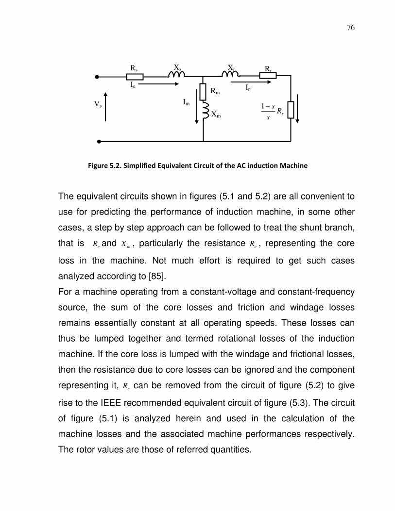
76
Figure 5.2. Simplified Equivalent Circuit of the AC induction Machine
The equivalent circuits shown in figures (5.1 and 5.2) are all convenient to
use for predicting the performance of induction machine, in some other
cases, a step by step approach can be followed to treat the shunt branch,
that is cR and mX , particularly the resistance cR , representing the core
loss in the machine. Not much effort is required to get such cases
analyzed according to [85].
For a machine operating from a constant-voltage and constant-frequency
source, the sum of the core losses and friction and windage losses
remains essentially constant at all operating speeds. These losses can
thus be lumped together and termed rotational losses of the induction
machine. If the core loss is lumped with the windage and frictional losses,
then the resistance due to core losses can be ignored and the component
representing it, cR can be removed from the circuit of figure (5.2) to give
rise to the IEEE recommended equivalent circuit of figure (5.3). The circuit
of figure (5.1) is analyzed herein and used in the calculation of the
machine losses and the associated machine performances respectively.
The rotor values are those of referred quantities.
Is
Vs Im
Xm
Rm Ir
Rr Xr Xs
Rs
rRs
s−1
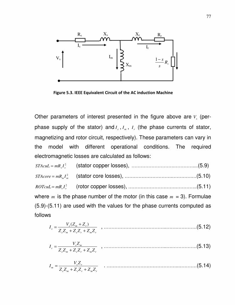
77
Figure 5.3. IEEE Equivalent Circuit of the AC induction Machine
Other parameters of interest presented in the figure above are sV (per-
phase supply of the stator) and sI , mI , rI (the phase currents of stator,
magnetizing and rotor circuit, respectively). These parameters can vary in
the model with different operational conditions. The required
electromagnetic losses are calculated as follows:
2
ss ImRSTAcuL = (stator copper losses), ……………………….…………....(5.9)
2
mm ImRSTAcore = (stator core losses), ………………………….………….…(5.10)
2
rr ImRROTcuL = (rotor copper losses), ………………………….…………..(5.11)
where m is the phase number of the motor (in this case m = 3). Formulae
(5.9)-(5.11) are used with the values for the phase currents computed as
follows
rmrsms
rmss
ZZZZZZ
ZZVI
++
+=
)( , …………………………………..…….………….(5.12)
rmrsms
msr
ZZZZZZ
ZVI
++=
, …………………………………..….…………….(5.13)
rmrsms
rsm
ZZZZZZ
ZVI
++= . ………………………………………..…………(5.14)
Rr Xr Xs
Rs
Is
Vs Im
Xm
Ir
rRs
s−1

78
Where sZ , mZ and rZ are the phase impedances of stator, magnetizing
and rotor circuit, respectively
mmmrrrsss jXRZjXsRZjXRZ +=+=+= ,/, ………………………………(5.15)
Finally, the leakage reactances sX , rX and mX in (5.15) are computed
by using the following formulae ,2,2,2 mmrrss fLXfLXfLX πππ === where sL ,
rL and mL are leakage inductance of stator, rotor and the magnetized
inductance respectively. In this work, various losses formula shown below
which were used in [10] are also adopted in calculating the associated
losses.
The iron loss ( FeP ) is principally made up of the hysteresis ( hysP ) and the
eddy current ( eddP ) losses.
fMB
P hyshys
2
10
= σ ……………………………………………….………….……(5.16)
MfB
P Feeddedd
22
1010
∆
= σ ………………………………………….……………(5.17)
MBf
fPPP FeeddhyseddhysFe
2
2
10
10
∆+=+= σσ …………………………………..(5.18)
and for squirrel induction machine , FerFesTFeyFeTot PPPP ++= …………….(5.19)
where
eddσ is eddy current loss coefficient
hysσ is hysteresis loss coefficient
B is the magnetic flux density,
Fe∆ is the thickness of lamination
f is the frequency and M is the mass.

79
,FeyP FesTP and FerP are loss components of yoke, stator teeth and rotor.
To distribute the total iron losses FeTotP between the stator and rotor a
factor ( sK ) is used such that: for stator we have FeTotsFes PKP = ……. (5.20)
and for the rotor we have ( ) FeTotsFer PKP −= 1 ……………………………….. (5.21)
Stator iron losses are in itself re-distributed between the teeth and yoke
components with another factor ( tK ) such that: for the yoke we have
FestFey PKP = …………………………………………………….……………………. (5.22)
and for the rotor we have ( ) FestFesT PKP −= 1 ………………..………….…(5.23)
5.3 LOSS ESTIMATION OF THE 7.5kW INDUCTION MACHINE
The values of the parameters of this 400V, 50 Hz, 10Hp machine having
4 poles, whose synchronous and measured rated speeds are 1500 rpm
and 1440 rpm with rated current 13.5A analyzed in this work are given in
Table 5.1 below.
Table 5.1: Induction Machine rating and Parameters [98]
10HP Induction Motor Parameters Value No of poles 4

80
Rated speed 1440 rpm Rated frequency ( f ) 50 Hz
Output power 7.5 KW Rated voltage 400 V Stator Current ( sI ) 13.4699 A
Stator Resistance ( sR ) 0.7384 Ω
Rotor Resistance ( rR, ) 0.7402 Ω
Stator Leakage Inductance ( sL ) 0.003045 H
Magnetizing Inductance ( mL ) 0.1241H
Excitation Current ( 0I ) 5.5534 A
Stator Core Loss Resistance ( cR ) 680.58 Ω
Motor inertia ( J ) 0.0343 Kgm2 Wind frictional coefficient ( F ) 0.000503 NmS Calculated rated values Rotor Current ( rI
, ) 11.6627 A Stator Core Loss Current ( cI ) 0.3393 A
Magnetizing Current ( mI ) 5.5430 A
Slip ( s ) 0.04 Rotor Leakage Inductance ( rL
, ) 0.003045 H Stator Leakage Inductance ( sL ) 0.003045 H
Magnetizing Inductance ( mL ) 0.1241H
Angle between sV and sI 28.90o
Shaft Load Torque ( shT ) 49.471 N-m
Developed electromagnetic torque ( eT ) 48.079 N-m
All the loss estimation of this 10HP induction machine has also been
summarized in table (5.2) while formulas for the detailed calculation are
provided as m-files in the appendices, the results obtained here followed
careful usage of some of these formulas:
Input power: θCosIVP ssin 3= ………………………………………………….……………….…. (5.24)
The input power of the induction machine is W 8158.91
Efficiency calculation:

81
%100*1
−=
in
losses
P
Pη ……………………………………………….…………
(5.25)
Losses calculation:
If power losses(Plosses), stator copper loss ( PSTAcuL), rotor copper loss
(PROTcuL), stator core loss (PSTAcore), Friction and windage losses (PFRIwin )
and stray load loss( PSTR ) are represented in this way, then;
Plosses = PSTAcuL + PROTcuL + PSTAcore + PFRIwin + PSTR …………………….. (5.26)
The Shaft Load Torque:
)( NmP
Tin
outSh
ω= ……………………………………………….…….………(5.27)
Air gap power:
s
RIP r
rAG
23= ……………………………………………….……….…….....…
(5.28)
Per-Phase Stator Core Loss Resistance (neglecting the stator impedance voltage drop):
c
sc
I
VR =
……………………………………………….………………...………
(5.29)
Per-Phase Stator Magnetizing Inductance:
m
sm
fI
VL
π2=
……………………………………………….…………..…..… ..(5.30)
Based on IEEE 1112-B standard [81], the PSTR value at 1 kW is 2.5% of
the full-load input power, dropping at 10kW to 2%, at 100kW to 1.5%, at
1000kW to 1%, and at 10MW to 0.5% as reported in [87, 88], the stray
load loss and rotational losses can be calculated .
Since the machine under study here is a 10 hp machine, therefore,
PSTR(IEEE) = W 18.163%0.2*8158.91 = ………………………………………….. (5.31)
However, in the IEC 34-2 standard, these losses were not measured but
were arbitrarily estimated to be equal to 0.5% of the full-load input power
[82, 83], so that PSTR(IEC) = W 40.795%5.0*8158.91 = ……………………….(5.32)

82
A suggested solution in Ontario Hydro’s simplified segregated loss
method assumed a value for a combined windage, friction and core
losses [84, 88]. The study recommends that these combined losses be
set to 3.5% of the input rated power which translates to:
WPP inROTaL *%5.3 = ……………………………………………….…………… (5.33)
Therefore, obtained rotational losses:
8158.91*%5.3=ROTaLP W 285.562= ……………………………………………… (5.34)
5.4 SEGREGATION AND ANALYSIS OF THE IM LOSSES The estimated losses are summarized in table (5.2) below and presented
in the following bar and pie charts for ease of understanding.
TABLE 5.2: Loss Segregation Obtained from Calculation
Losses Segregation Calculated Value (W)
Input Power (Pin) 8159.2

83
Stator Copper Loss 400.8250
Rotor Copper Loss 302.0875
Stator Core loss 235.0474
Friction and Windage Losses 50.5247
Stray Losses (PstrayIEEE-12B Standard) 163.1840
Total Losses (Watts) 1151.7
Output Power (Pout) 6968.5
1 2 3 4 50
50
100
150
200
250
300
350
400
450
Class of Losses
Losses
([w
atts]
)
1- STAcuL2- ROTcuL3- STAcore4- STRieee5- FRIwin
Figure 5.4. Bar chart representing loss segregation of 10HP induction machine
5.5 PERFORMANCE CHARACTERISTIC OF THE 10HP INDUCTION MACHINE
When the parameters of table 5.1 are further used for the equivalent
circuit of figure 5.1, steady state performance curves are generated as
indicated in figures 5.5 to 5.9.

84
0 500 1000 15000
20
40
60
80
100
120
140
160
180Torque vs speed curve for IM
Speed in RPM
Torq
ue in N
-m
Figure 5.5. Torque against speed characteristics for the 10HP induction machine
0 500 1000 15000
0.2
0.4
0.6
0.8
1
1.2
1.4
1.6
1.8
2x 10
4Power vs speed curve for IM
Speed in RPM
Pow
er in
watts
Figure 5.6. Power against speed characteristics for the 10HP induction machine

85
0 500 1000 15000
10
20
30
40
50
60
70stator current vs speed curve for IM
Speed in RPM
sta
tor
cu
rre
nt
in A
mp
ere
s
Figure 5.7. Stator current against Speed for 10HP induction machine
0 0.1 0.2 0.3 0.4 0.5 0.6 0.7 0.8 0.9 10
20
40
60
80
100
120
140
160
180Torque vs slip curve for IM
Torq
ue in N
-m
Slip in p.u.
Figure 5.8. Graph showing the Torque-Slip characteristics for 10HP induction machine
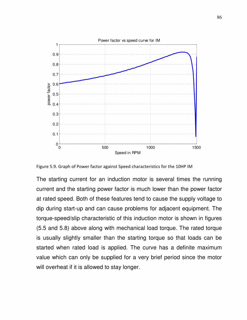
86
0 500 1000 15000
0.1
0.2
0.3
0.4
0.5
0.6
0.7
0.8
0.9
1Power factor vs speed curve for IM
Speed in RPM
pow
er
facto
r
Figure 5.9. Graph of Power factor against Speed characteristics for the 10HP IM
The starting current for an induction motor is several times the running
current and the starting power factor is much lower than the power factor
at rated speed. Both of these features tend to cause the supply voltage to
dip during start-up and can cause problems for adjacent equipment. The
torque-speed/slip characteristic of this induction motor is shown in figures
(5.5 and 5.8) above along with mechanical load torque. The rated torque
is usually slightly smaller than the starting torque so that loads can be
started when rated load is applied. The curve has a definite maximum
value which can only be supplied for a very brief period since the motor
will overheat if it is allowed to stay longer.

87
In figure (5.7), the response of current to the speed is plotted. The starting
current is several times larger than the rated current since the back emf
induced by Faraday’s law grows smaller as the rotor speed decreases.
Whenever a squirrel-cage induction motor is started, the electrical system
experiences a current surge while the mechanical system experiences
torque surge. With line voltage applied to the machine, the current can be
anywhere from four to ten times the machine’s full load current. The
magnitude of the torque (turning force) that the driven equipment sees
can be above 200% of the machine’s full load torque [89]. These
wastages of power due to losses account for a reduced internal and
thermal efficiency of the machine [90, 91]. The associated current and
torque surges can be reduced substantially by reducing the voltage
supplied to the machine during starting as one of the most noticeable
effects of full voltage starting is the dimming or flickering of light during
starting.
5.6.1 Motor Efficiency /Losses
The difference - watts loss is due to electrical losses plus those due to
friction and windage. Even though higher horsepower motors are typically
more efficient, their losses are significant and should not be ignored. In
fact, according to [94] higher horsepower motors offer the greatest
savings potential for the least analysis effort, since just one motor can
save more energy than several smaller motors.
5.6.2 Determination of Motor Efficiency
Every AC motor has five components of watts losses which are the
reasons for its inefficiency. Watts losses are converted into heat which is

88
dissipated by the motor frame aided by internal or external fans. Stator
and rotor RI 2 losses are caused by current flowing through the motor
winding and are proportional to the current squared times the winding
resistance ( RI 2 ). Iron losses are mainly confined to the laminated core of
the stator and rotor and can be reduced by utilizing steels with low core
loss characteristics found in high grade silicon steel. Friction and windage
loss is due to all sources of friction and air movement in the motor and
may be appreciable in large high-speed or totally enclosed fan-cooled
motors. The stray load loss is due mainly to high frequency flux pulsations
caused by design and manufacturing variations.
5.6.3 Improving Efficiency by Minimizing Watts Losses Improvements
in motor efficiency can be achieved without compromising motor
performance at higher cost within the limits of existing design and
manufacturing technology. The formula for efficiency in equation (5.47)
shows that any improvement in motor efficiency must be the result of
reducing watts losses. In terms of the existing state of electric motor
technology, a reduction in watts losses can be achieved in various ways.
All of these changes to reduce motor losses are possible with existing
motor design and manufacturing technology. They would, however,
require additional materials and/or the use of higher quality materials and
improved manufacturing processes resulting in increased motor cost. In
summary, we can say that reduced losses imply improved efficiency.

89
Table 5.3: Efficiency improvement schemes [94]
Watts Loss Area Efficiency Improvement 1 Iron Use of thinner gauge, lower loss core steel
reduces eddy current losses. Longer core adds more steel to the design, which reduces losses due to lower operating flux densities.
2 Stator RI 2 Use of more copper and larger conductors increases cross sectional area of stator windings. This lowers resistance ( R ) of the windings and reduces losses due to current flow ( I ).
3 Rotor RI 2 Use of larger rotor conductor bars increases size of cross section, lowering conductor resistance ( R ) and losses due to current flow ( I ).
4 Friction/ Windage Use of low loss fan design reduces losses due to air movement.
5 Stray Load Loss Use of optimized design and strict quality control procedures minimizes stray load losses.
5.7 THE EFFECTS OF TEMPERATURE
Temperature effect in induction machine has a very important influence in
the assessment of the machines performance. Many works could not
consider the effects due to the difficulty encountered in the measurements.
This difficulty according to [95] is due to the strong coupling between the
electrical and thermal phenomena inherent in the machine. Attempts at
modelling it by the variation of the stator and rotor equivalent resistances
as a function of their average temperatures which were measured directly
90
using a microprocessor-based data acquisition apparatus was carried out
in [77]. The measured resistance mR at the test temperature tT is
corrected to a specified temperature sT as follows;
..........................................................................................................KT
KTRR
t
stm
+
+= ……(5.48)
where mR is the corrected resistance at sT , and 5.234=K and 225 for
copper and aluminum respectively [32, 77].
In induction motor thermal monitoring by [90], the rotor temperature was
monitored from its resistance identification and then its temperature
dependence given by:
..............................................................................................].........1[0 TRR ∆+= α …..(5.49)
where 0R is resistance at reference temperature 25 C0 , however 20 C
0
is used herein, α is resistance temperature coefficient and T∆ is
temperature increase. The resistance method allows for the measurement
of stator winding temperatures. However the main source of error in the
use of the resistance method is from impurities associated with copper.
91
CHAPTER SIX
THERMAL MODELLING AND COMPUTER SIMULATION
6.1 THE HEAT BALANCE EQUATIONS
In the lumped parameter thermal circuit analysis, it is often assumed that
the temperature gradient with certain parts of the machine is negligible.
According to [60] this assumption can only be made if the internal
resistance to the heat transfer is small compared with the external
resistance. The Biot number iB , is usually used for determining the validity
of this assumption. In the case where internal conduction resistance is
compared with external convective resistance, iB is defined as:
...............................................................................................................s
c
ik
LhB = ………(6.1)
where sk is the thermal conductivity of the solid material
L is the characteristic length of the solid body
ch is the convective heat transfer coefficient.
The criterion 1.0∠iB ensures that the internal temperature will not differ
and in the words of [96], the assumption of uniform temperature is
acceptable except for the early times of the step change in temperature
and for such, the time for the change is localized in a thin ‘skin’ near the
fluid or solid surface.
6.2 THERMAL MODELS AND NETWORK THEORY
In modelling a thermal network, the material is discretized giving rise to
aggregates of thermal elements that join at a given node through thermal
resistances. Inadequate discretisation has been considered in [97] as one
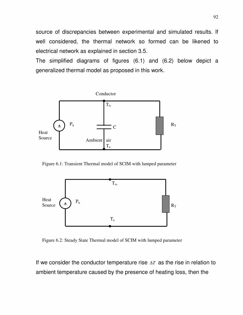
92
source of discrepancies between experimental and simulated results. If
well considered, the thermal network so formed can be likened to
electrical network as explained in section 3.5.
The simplified diagrams of figures (6.1) and (6.2) below depict a
generalized thermal model as proposed in this work.
If we consider the conductor temperature rise T∆ as the rise in relation to
ambient temperature caused by the presence of heating loss, then the
Figure 6.1: Transient Thermal model of SCIM with lumped parameter
RT
Heat
Source
Tts
C
Ambient air
Ta
Ps
Conductor
Tss
RT
Heat
Source
Ta
Ps
Figure 6.2: Steady State Thermal model of SCIM with lumped parameter

93
temperature rise is generally given by aTTT −=∆ hence in figure 6.1 we
have that atsts TTT −=∆ while in figure 6.2 we have that Tsss RPTT =∆=∆ . This
will thus give us 0=−∆
+∆
S
T
PR
T
dt
TdC ……………………………………….(6.2)
The ambient air temperature aT , serves as the thermal reference while a
deviation from the reference, that is, a rise in temperature denotes the
machine elements. Assuming that we have ‘ N ’ number of loads singly
linked to other nodes via thermal resistances baR , in which ba and are the
number of the nodes, with baR , as the thermal resistance between the
reference and node ‘b ’ then the steady-state rise in temperature at the
node ‘a ’ can be derived from the relation below:
............................................. 1 a 01 ,,
∑=
=
+−=
N
b ba
b
ba
aa
R
T
R
TP ……………………….(6.3)
Where
b. anda nodes adjoining twobetween resistance thermal
a node of re temperatuthe
a nodeat generationheat the
, =
=
=
ba
a
a
R
T
P
For multinode consideration, 1T to NT represent the temperature rises of
each node while 1P to NP represent the losses at the various nodes. The
matrix defined by ‘G ’ in equation (6.4) is a conductance matrix which
when joined with the column vectors represented by TP and TT as given
below give rise to equation ( 6.5 ) which finally leads to a stationary
solution using equation (6.6).

94
−−−−
−−−−
−−−−
−−−−
−−−−
=
∑
∑
∑
∑
∑
=
=
=
=
=
N
a aNNNNN
N
N
a a
N
N
a a
N
N
a a
N
N
a a
RRRRR
RRRRR
RRRRR
RRRRR
RRRRR
G
1 ,4,3,2,1,
,41 ,43,42,41,4
,34,31 ,32,31,3
,24,23,21 ,21,2
,14,13,12,11 ,1
1...
1111..................
1...
1111
1...
1111
1...
1111
1...
1111
,……………………………... (6.4)
=
N
T
P
P
P
P
P
P
...4
3
2
1
and
=
N
T
T
T
T
T
T
T
...4
3
2
1
TT GTP = ………………………….……………………………………….. (6.5)
Hence TT PGT 1−= ………………………………………………………..………… (6.6)
The SIM thermal network in full form as shown in figure (6.3) has a total of
twelve nodes and fifteen thermal resistances, while that of LIM as shown
in figure (6.4) has fourteen nodes and eighteen thermal resistances. It
was assumed in [15] that the heat transferred from the rotor winding
through the air-gap goes directly to the stator winding with negligible
impact on the stator teeth, however this assumption did not go down well
with the LIM model here as the teeth is fully considered and the effects
studied alongside others. Hence, the rotor part of the machine is divided
into the rotor iron, rotor windings, rotor teeth and end rings while the
stator of the machine has networks for the stator iron, stator winding, and

95
end winding together with the stator teeth. The connection of the above
mentioned networks for rotor, stator and frame gives rise to the thermal
network models of figures (6.3 and 6.4) as shown below. The separate
temperatures of the nodes are evaluated using this set of heat balance
equation as given below.
( ) 1 b a, 1
=
−−= ba
ab
aa TTR
Pdt
dTC ………………..……………………….……(6.7)
Where
a nodeat generationheat the
b. anda nodes adjoining twobetween resistance thermal
a node of re temperatuthe
a node of ecapacitanc thermal
=
=
=
=
a
ab
a
a
P
R
T
C
The power losses ( 1P - 11P ) associated with the model of figure (6.3) are
outlined in equations (6.8 – 6.20). However, in the simulation for the half
model of the induction machine, equations (6.8 – 6.15) representing ( 1P )
to ( 8P ) are used. This is equivalent to losses equations ( 1P - 8P ) and are
shown at the right hand side of figure (6.3) with shaded resistors.

96
8
Figure 6.3: Thermal network model for the squirrel cage induction machine
SIM Half Model --Considered
Rotor Iron
Rotor bar
(winding)
End-ring
End-winding
End-winding
Frame
Stator lamination
Stator winding
Ambient
R12
P2
T1a
R8c
T1b
R1b
R23
P3 P11
10
C9
C4 C3
P5
R56
P6
R69 R78
P7
C5
R25
R311 R1011
C6
C7
C11
C2
C1
R34
P4
R910
R48
End-ring
P9
R10a
R67
T1c

97
In the case of the complete (LIM) model, equations (6.16 and 6.17) for ( 3P )
and ( 6P ) are respectively modified as ( 3'
P ) and ( 6'
P ) while equations (6.18
– 6.20) for ( 9P ), ( 10P ) and ( 11P ) as derived from the complete model are
added so as to obtain the following set of equations.
( ) ( ) ........................................................11
1
1
21
12
111 b
b
TTR
TTRdt
dTCP −+−+= ………… (6.8)
( ) ( ) ( ).....11152
25
32
23
12
12
222 TT
RTT
RTT
Rdt
dTCP −+−+−+= ………………. ………… (6.9)
( ) ( ) ..........................................11
43
34
23
32
333 TT
RTT
Rdt
dTCP −+−+= ……………………...(6.10)
( ) ( ) ............11
34
34
84
48
444 TT
RTT
Rdt
dTCP −+−+= ……………………………………..(6.11)
( ) ( ) ...........................................11
65
56
25
52
555 TT
RTT
Rdt
dTCP −+−+= …………………..(6.12)
( ) ( ) .........................11
76
67
56
65
666 TT
RTT
Rdt
dTCP −+−+= ……………………………....(6.13)
( ) ( ) ...................................11
87
78
67
76
777 TT
RTT
Rdt
dTCP −+−+= ………………………..…(6.14)
( ) ( ) ( ) ...........111
8
8
48
84
78
87
888 c
c
TTR
TTR
TTRdt
dTCP −+−+−+= ……………………..… (6.15)
( ) ( ) ( ) ................................111
113
311
43
34
23
32
333
' TTR
TTR
TTRdt
dTCP −+−+−+= ………... (6.16)
( ) ( ) ( ) ......................111
96
69
76
67
56
65
666
'TT
RTT
RTT
Rdt
dTCP −+−+−+= … …………...(6.17)
( ) ( ) ........................................11
109
910
69
69
999 TT
RTT
Rdt
dTCP −+−+= …………………. (6.18)
( ) ( ) ( )........11110
10
910
910
1110
1011
101010 a
a
TTR
TTR
TTRdt
dTCP −+−+−+= ………………… (6.19)
( ) ( ) .................................11
1011
1011
311
311
111111 TT
RTT
Rdt
dTCP −+−+= …….…………….(6.20)

98
Figure 6.4: Thermal network model for the squirrel cage induction machine
LIM Full Model
11
C4
C2
C1
R35 P5
R810
R511
End-ring
P8
R10a
Tc
P12
R312
R1213
C12 Stator teeth
P13
Rotor teeth
C13
R713
R79
Rotor Iron
Rotor bar
(winding)
End-ring
End-winding
End-winding
Frame
Stator lamination
Stator winding
Ambient
P1
R12
P2
Ta
R11c
Tb
R1b
R23
P3
P4 10
C8
C5
C3
P6
R67
P7
R78
R911
P9
C6
R26
R34 R410
C7
C9

99
6.3 THE TRANSIENT STATE ANALYSIS
The general transient equation for thermal network system of ‘ N ’ nodes
linking others through thermal resistances baR , is represented as follows:
[ ] [ ]dt
TdCa = 1 a
1 ,,
∑=
=
+−
N
b ba
b
ba
aa
R
T
R
TP ……………………………………….…(6.21)
where
a nodeat generationheat the
b. anda nodes adjoining twobetween resistance thermal
a node of re temperatuthe
a node of ecapacitanc thermal
,
=
=
=
=
a
ba
a
a
P
R
T
C
The existence of thermal capacitance in the network demands that a
thermal capacitance matrix as given below will be incorporated.
.....................................................................
...0000
..................
0...000
0...000
0...000
0...000
4
3
2
1
=
NC
C
C
C
C
C ……. (6.22)
Hence we have,
[ ] [ ] [ ] [ ][ ]TGPdt
TdC −= ……………………………………………………………...(6.23)
Or
[ ] [ ] [ ][ ] ................................................................ ][][ 11TGCPC
dt
Td −−−= ……………...(6.24)
where
[ ][ ][ ] generators thermalofmatrix column a
esconductanc internodal ofmatrix square a
escapacitanc thermalofmatrix column
=
=
=
P
G
C
100
The power associated with each thermal node is expressed as shown in
this system of algebraic and differential equations which sum up the
thermal behaviour of the developed thermal model of figure 6.4.
( ) ( ) ........................................................11
1
1
21
12
111 b
b
TTR
TTRdt
dTCP −+−+= …………..(6.25)
( ) ( ) ( ) ....................................111
62
26
32
23
12
12
222 TT
RTT
RTT
Rdt
dTCP −+−+−+= …….. (6.26)
( ) ( ) ( ) ( ) ..............1111
123
312
43
34
53
35
23
32
333 TT
RTT
RTT
RTT
Rdt
dTCP −+−+−+−+= ………. (6.27)
( ) ( ) ...........................................................11
34
34
104
410
444 TT
RTT
Rdt
dTCP −+−+= ……..(6.28)
( ) ( ) ..........................................................11
115
511
35
53
555 TT
RTT
Rdt
dTCP −+−+= ……. (6.29)
( ) ( ) ..................................................11
26
62
76
67
666 TT
RTT
Rdt
dTCP −+−+= …………… (6.30)
( ) ( ) ( ) ( ) .............1111
137
713
97
79
87
78
67
67
777 TT
RTT
RTT
RTT
Rdt
dTCP −+−+−+−+= ……… (6.31)
( ) ( ) .......................................................11
108
810
78
78
888 TT
RTT
Rdt
dTCP −+−+= ……….. (6.32)
( ) ( ) ....................................................11
119
911
79
79
999 TT
RTT
Rdt
dTCP −+−+= ………… (6.33)
( ) ( ) ( ) .....................111
10
10
810
810
410
410
101010 a
a
TTR
TTR
TTRdt
dTCP −+−+−+= ………… (6.34)
( ) ( ) ( )..........111911
119
11
11
511
511
111111 TT
RTT
RTT
Rdt
dTCP c
c
−+−+−+= …………… ……..(6.35)
( ) ( ) ............................................11
1312
1213
312
312
121212 TT
RTT
Rdt
dTCP −+−+= ………… (6.36)
( ) ( ) .........................................11
1213
1213
713
713
131313 TT
RTT
Rdt
dTCP −+−+= ……………(6.37)

101
The constants ,aT bT and cT are the ambient temperature values and are
equal, the equations are further rearranged to make the differential the
subject as shown below. Matlab programs [98 - 101] are developed to
solve the steady state and transient state mathematical models of the
machine.
( ) ( ) .............................................111
1
1
21
12
1
1
1
−−−−= b
b
TTR
TTR
PCdt
dT……………………(6.38)
( ) ( ) ( ) .............................1111
62
26
32
23
12
12
2
2
2
−−−−−−= TT
RTT
RTT
RP
Cdt
dT………..…(6.39)
( ) ( ) ( ) ( ) ........11111
123
312
43
34
53
35
23
32
3
3
3
−−−−−−−−= TT
RTT
RTT
RTT
RP
Cdt
dT…………...(6.40)
( ) ( ) ............................................111
34
34
104
410
4
4
4
−−−−= TT
RTT
RP
Cdt
dT………………(6.41)
( ) ( ) .................................................111
115
511
35
53
5
5
5
−−−−= TT
RTT
RP
Cdt
dT……………(6.42)
( ) ( ) ...............................................111
26
62
76
67
6
6
6
−−−−= TT
RTT
RP
Cdt
dT…………..…(6.43)
( ) ( ) ( ) ( ) ..........11111
137
713
97
79
87
78
67
67
7
7
7
−−−−−−−−= TT
RTT
RTT
RTT
RP
Cdt
dT…………(6.44)
( ) ( ) ...............................................111
108
810
78
78
8
8
8
−−−−= θT
RTT
RP
Cdt
dT…………....(6.45)
( ) ( ) .............................................111
119
911
79
79
9
9
1
−−−−= TT
RTT
RP
Cdt
dT……………...(6.46)
( ) ( ) ( ) .........................1111
10
10
810
810
410
410
10
10
10
−−−−−−= a
a
TTR
TTR
TTR
PCdt
dT……..(6.47)
( ) ( ) ( ) .......1111
911
119
11
11
511
511
11
11
11
−−−−−−= TT
RTT
RTT
RP
Cdt
dTc
c
……………………(6.48)

102
( ) ( ) ..............................................111
1312
1213
312
312
12
12
12
−−−−= TT
RTT
RP
Cdt
dT …….(6.49)
( ) ( ) .............................................111
1213
1213
713
713
13
13
13
−−−−= TT
RTT
RP
Cdt
dT. ……..(6.50)
Having arranged them in that form, the next thing is to put them in the
matrix form and according to this expression:
[ ] [ ] [ ] [ ][ ] ........................................................ *11
TGCPCT tttt
−−•
−=
…………...........(6.51)
where
[ ]
1
13
12
11
10
9
8
7
6
5
4
3
2
1
1
000000000000
000000000000
000000000000
000000000000
000000000000
000000000000
000000000000
000000000000
000000000000
000000000000
000000000000
000000000000
000000000000
−
−
=
C
C
C
C
C
C
C
C
C
C
C
C
C
Cand t
;
T
T
T
T
T
T
T
T
T
T
T
T
13
12
11
10
9
8
7
6
5
4
3
2
1
=
•
•
•
•
•
•
•
•
•
•
•
•
•
•
T
T

103
[ ]
+
=
13
12
11
10
9
8
7
6
5
4
3
2
11
*
*
*
P
P
GT
GT
P
P
P
P
P
P
P
P
GTP
P
cc
aa
bb
t , [ ]
=
13
12
11
10
9
8
7
6
5
4
3
2
1
T
T
T
T
T
T
T
T
T
T
T
T
T
T and
[ ] (6.52)
0000000000
0000000000
0000000000
0000000000
0000000000
0000000000
00000000
0000000000
0000000000
0000000000
00000000
000000000
00000000000
13131312137
12131212123
1111119115
1010108104
9119997
8108887
71379787776
676662
5115553
4104443
31235343332
26232221
1211
−−
−−
−−
−−
−−
−−
−−−−
−−
−−
−−
−−−−
−−−
−
=
GGG
GGG
GGG
GGG
GGG
GGG
GGGCG
GGG
GGG
GGG
GGGGG
GGGG
GG
Gt
Some of the entries of the tG -matrix are given as follows:
..........................................................................................1211 GGG b += ……………...(6.53)
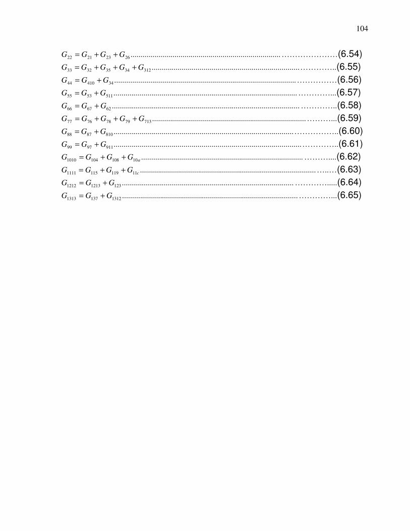
104
...........................................................................26232122 GGGG ++= …………………(6.54)
..........................................................................31234353233 GGGGG +++= …………..(6.55)
...........................................................................................3441044 GGG += ……………(6.56)
............................................................................................5115355 GGG += …………...(6.57)
..............................................................................................626766 GGG += …………..(6.58)
.............................................................................71379787677 GGGGG +++= ………...(6.59)
..........................................................................................8108788 GGG += ……………..(6.60)
..............................................................................................9119799 GGG += …………..(6.61)
.................................................................................101081041010 aGGGG ++= ………....(6.62)
........................................................................................111191151111 cGGGG ++= …..…(6.63)
......................................................................................12312131212 GGG += ………….....(6.64)
........................................................................................13121371313 GGG += …………...(6.65)

105
6.4 THE STEADY STATE ANALYSIS
Equation (6.23) holds firm for the induction motor when it is rotating.
However, at stand still, a different conductance matrix [ ]ssG is used
because of the attendant change in the value of the convective elements
of the branch thermal impedances. The stand still equation when there is
no supply (no heat generation), is given as:
[ ] [ ] [ ] [ ][ ]TGPdt
TdC ss −= ……………………………………………………………….. (6.66)
During the steady state, the thermal capacitance is at maximum so that
the derivative [ ]
0=dt
Td hence loses its contribution just as it renders
equation(6.21) as ............. 1.......N a 1 ,
∑=
=
−=
N
b ba
ba
aR
TTP ………………..(6.67)
Hence the algebraic steady-state temperature rise in the proposed
thermal network model in matrix form can be written as follows:
[ ] [ ][ ] ................................................................................... ttt TGP = ……………. …….(6.68)
So that we have on arranging
[ ] [ ] [ ] ........................................................................................... 1
ttt PGT−
= …………...(6.69)
where all the three variables are also defined thus;
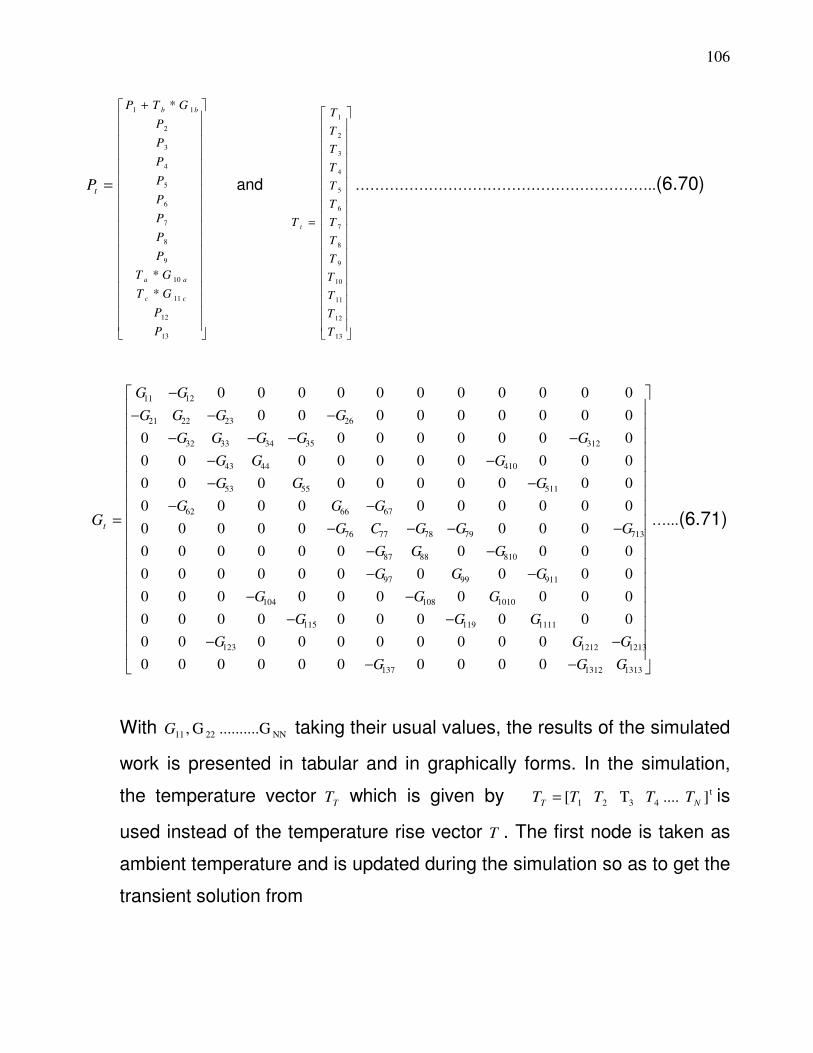
106
=tP
+
13
12
11
10
9
8
7
6
5
4
3
2
11
*
*
*
P
P
GT
GT
P
P
P
P
P
P
P
P
GTP
cc
aa
bb
and
=
13
12
11
10
9
8
7
6
5
4
3
2
1
T
T
T
T
T
T
T
T
T
T
T
T
T
T t
……………………………………………………..(6.70)
=tG
−−
−−
−−
−−
−−
−−
−−−−
−−
−−
−−
−−−−
−−−
−
13131312137
12131212123
1111119115
1010108104
9119997
8108887
71379787776
676662
5115553
4104443
31235343332
26232221
1211
0000000000
0000000000
0000000000
0000000000
0000000000
0000000000
00000000
0000000000
0000000000
0000000000
00000000
000000000
00000000000
GGG
GGG
GGG
GGG
GGG
GGG
GGGCG
GGG
GGG
GGG
GGGGG
GGGG
GG
…...(6.71)
With NN2211 G.......... G ,G taking their usual values, the results of the simulated
work is presented in tabular and in graphically forms. In the simulation,
the temperature vector TT which is given by t
4321 ] .... T [ NT TTTTT = is
used instead of the temperature rise vector T . The first node is taken as
ambient temperature and is updated during the simulation so as to get the
transient solution from
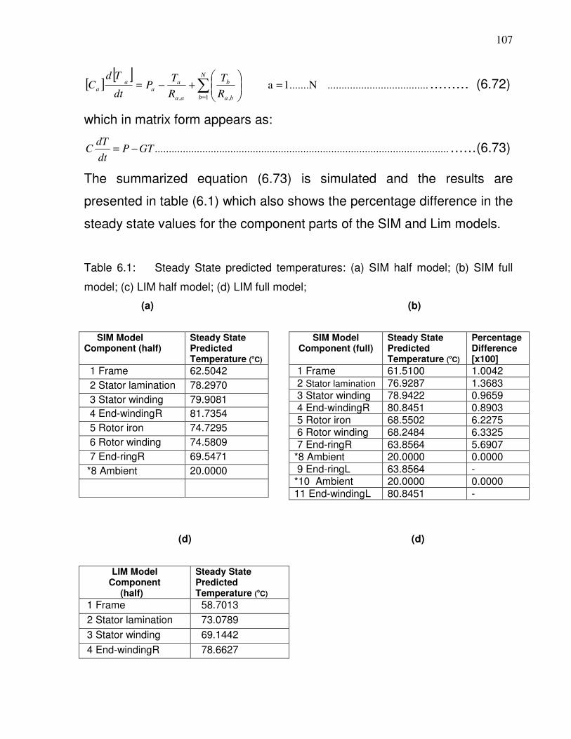
107
[ ][ ]dt
TdC a
a = .................................... 1.......N a 1 ,,
∑=
=
+−
N
b ba
b
aa
aa
R
T
R
TP ……… (6.72)
which in matrix form appears as:
.........................................................................................................GTPdt
dTC −= ……(6.73)
The summarized equation (6.73) is simulated and the results are
presented in table (6.1) which also shows the percentage difference in the
steady state values for the component parts of the SIM and Lim models.
Table 6.1: Steady State predicted temperatures: (a) SIM half model; (b) SIM full
model; (c) LIM half model; (d) LIM full model;
(a) (b)
(d) (d)
SIM Model Component (full)
Steady State Predicted Temperature (o
C)
Percentage Difference [x100]
1 Frame 61.5100 1.0042 2 Stator lamination 76.9287 1.3683 3 Stator winding 78.9422 0.9659 4 End-windingR 80.8451 0.8903 5 Rotor iron 68.5502 6.2275 6 Rotor winding 68.2484 6.3325 7 End-ringR 63.8564 5.6907 *8 Ambient 20.0000 0.0000 9 End-ringL 63.8564 - *10 Ambient 20.0000 0.0000 11 End-windingL 80.8451 -
SIM Model Component (half)
Steady State Predicted Temperature (o
C)
1 Frame 62.5042
2 Stator lamination 78.2970
3 Stator winding 79.9081
4 End-windingR 81.7354
5 Rotor iron 74.7295
6 Rotor winding 74.5809
7 End-ringR 69.5471
*8 Ambient 20.0000
LIM Model Component
(half)
Steady State Predicted Temperature (o
C)
1 Frame 58.7013
2 Stator lamination 73.0789
3 Stator winding 69.1442
4 End-windingR 78.6627

108
The bar charts of figures 6.5 and
6.6 represent the percentage
difference in predicted steady state
temperature rise of the component
parts. It is very clear that the
components of the LIM model have higher percentages of the steady
state temperature rise than the SIM model.
1 2 3 4 5 6 70
1
2
3
4
5
6
7
Model component [SIM]
Perc
enta
ge d
iffe
rence X
10
Frame 1Stator lamination 2Stator winding 3End windingR 4Rotor iron 5Rotor winding 6End ringR 7
5 Rotor iron 78.1632
6 Rotor winding 75.6776
7 End-ringR 70.0144
*8 Ambient 20.0000
9 Stator teeth 71.7736
10 Rotor teeth 78.0752
* Not shown on the graph
LIM Model Component
(full)
Steady State Predicted Temperature (o
C)
Percentage Difference [x100]
1 Frame 61.1247 2.4234
2 Stator lamination 76.4032 3.3243
3 Stator winding 74.1461 5.0019
4 End-windingR 83.2488 4.5861
5 Rotor iron 83.0035 4.8403
6 Rotor winding 83.6902 8.0126
7 End-ringR 78.0733 8.0589
*8 Ambient 20.0000 0.0000
9 End-ringL 56.0439 -
*10 Ambient 20.0000 0.0000
11 End-windingL 82.2513 -
12 Stator teeth 76.7514 4.9778
13 Rotor teeth 82.9178 4.8426
Figure 6.5: Percentage difference in component steady state
temperature for the half and full SIM model

109
1 2 3 4 5 6 7 8 90
1
2
3
4
5
6
7
8
9
Model component [LIM]
Perc
enta
ge d
iffe
ren
ce
x1
0
Frame 1
Stator lamination 2
Stator winding 3
End windingR 4
Rotor iron 5
Rotor winding 6
End ringR 7
Stator teeth 8
Rotor teeth 9
Figure 6.6: Percentage difference in component steady state
temperature for the half and full LIM model
6 .5 TRANSIENT STATE ANALYSIS RESULTS
Here, the graphs of the transient state analysis are presented to show the
rise in temperature of the component parts with time.
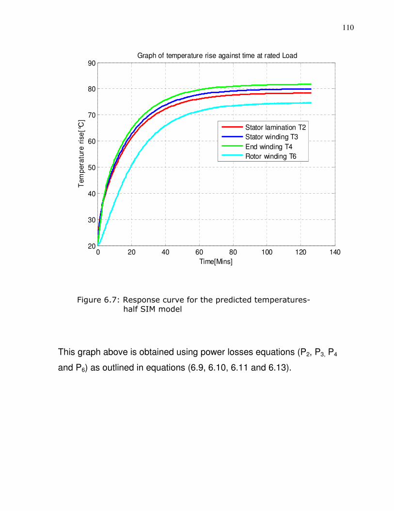
110
0 20 40 60 80 100 120 14020
30
40
50
60
70
80
90
Time[Mins]
Tem
pera
ture
ris
e[°
C]
Graph of temperature rise against time at rated Load
Stator lamination T2
Stator winding T3
End winding T4
Rotor winding T6
This graph above is obtained using power losses equations (P2, P3, P4
and P6) as outlined in equations (6.9, 6.10, 6.11 and 6.13).
Figure 6.7: Response curve for the predicted temperatures- half SIM model

111
0 20 40 60 80 100 120 14020
30
40
50
60
70
80
Time[Mins]
Te
mp
era
ture
ris
e[°
C]
Graph of temperature rise against time at rated load
Rotor iron T5
End Ring T7
Frame T1
This graph above is obtained using power losses equations (P5, P7, and
P1) as outlined in equations (6.12, 6.14, and 6.8).
Figure 6.8: Response curve for the predicted temperatures- half SIM model continued
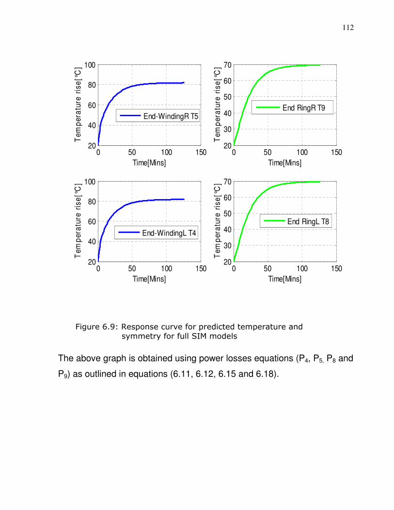
112
0 50 100 15020
40
60
80
100
Time[Mins]
Te
mp
era
ture
ris
e[°
C]
End-WindingR T5
0 50 100 15020
30
40
50
60
70
Time[Mins]
Te
mp
era
ture
ris
e[°
C]
End RingR T9
0 50 100 15020
40
60
80
100
Time[Mins]
Te
mp
era
ture
ris
e[°
C]
End-WindingL T4
0 50 100 15020
30
40
50
60
70
Time[Mins]
Te
mp
era
ture
ris
e[°
C]
End RingL T8
The above graph is obtained using power losses equations (P4, P5, P8 and
P9) as outlined in equations (6.11, 6.12, 6.15 and 6.18).
Figure 6.9: Response curve for predicted temperature and symmetry for full SIM models

113
0 20 40 60 80 100 120 14020
30
40
50
60
70
80
90
Time[Mins]
Te
mp
era
ture
ris
e[°
C]
Graph of temperature rise against time at rated Load
Stator lamination T2
Stator winding T3
End windingL T4
Rotor iron T6
This graph above is obtained using power losses equations (P2, P3, P4
and P6) as outlined in equations (6.26, 6.27, 6.28 and 6.30).
Figure 6.10: Response curve for the predicted transient state temperatures for LIM

114
0 20 40 60 80 100 120 14020
30
40
50
60
70
80
90
Time[Mins]
Te
mp
era
ture
ris
e[°
C]
Graph of temperature rise against time at rated load
End windingR T5
Rotor winding T7
Frame T1
End-ringL T8
The above graph is obtained using power losses equations (P1, P7, P5 and
P8) as outlined in equations (6.25, 6.31, 6.29 and 6.32).
Figure 6.11: Response curve for the predicted temperatures for LIM continued

115
0 20 40 60 80 100 120 14020
30
40
50
60
70
80
90
Time[Mins]
Te
mp
era
ture
ris
e[°
C]
Graph of temperature rise against time at rated load
End ringR T9
Ambient
Stator teeth T12
Rotor teeth T13
Figure 6.12: Response curves for the predicted transient state temperature rise for LIM continued
The above graph is obtained using power losses equations (P9, P12, and
P13) as outlined in equations (6.33, 6.36, and 6.37).

116
0 20 40 60 80 100 120 14020
30
40
50
60
70
80
Time[Mins]
Te
mp
era
ture
ris
e[°
C]
Graph of temperature rise against time at rated load
End ringR T9
End ringL T8
The above graph is obtained using power losses equations (P8 and P9) as
outlined in equations (6.32 and 6.33)
Figure 6.13: Comparing the response curves to show extent of difference in symmetry in end-ring of LIM model
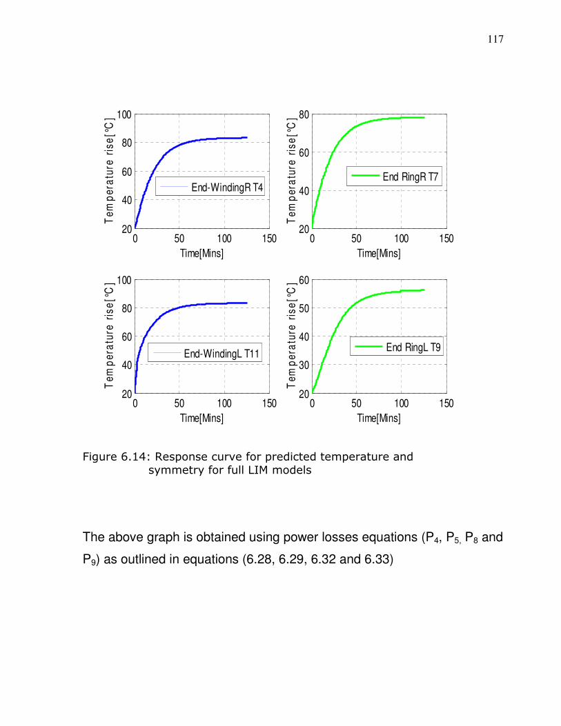
117
0 50 100 15020
40
60
80
100
Time[Mins]
Te
mp
era
ture
ris
e[°
C]
0 50 100 15020
40
60
80
Time[Mins]
Te
mp
era
ture
ris
e[°
C]
0 50 100 15020
40
60
80
100
Time[Mins]
Te
mp
era
ture
ris
e[°
C]
0 50 100 15020
30
40
50
60
Time[Mins]
Te
mp
era
ture
ris
e[°
C]
End-WindingR T4End RingR T7
End-WindingL T11End RingL T9
Figure 6.14: Response curve for predicted temperature and symmetry for full LIM models
The above graph is obtained using power losses equations (P4, P5, P8 and
P9) as outlined in equations (6.28, 6.29, 6.32 and 6.33)

118
6 .6 DISCUSSION OF RESULTS
It is obvious from table 6.2(a) representing SIM half model that the
predicted steady state temperature values recorded are slightly less than
that obtained from table 6.2(b) representing SIM full model.
However, in table 6.2(b), the predicted steady state temperature values
recorded for SIM full model shows that thermal symmetry effect was at
play. This is easily noticed when end ring and end winding steady state
temperature values are considered.
From table 6.2(c) representing LIM half model, the predicted steady state
temperature values recorded are also less than that obtained from table
6.2(d) representing LIM full model with that of left end ring giving a
reasonable difference.
In table 6.2(c), the predicted steady state temperature values recorded for
LIM full model shows that the effect of thermal symmetry cannot be
noticed again. This is easily observed when end ring, end winding, stator
teeth and rotor teeth steady state temperature values are considered. By
extension, the higher the size of the machine, the more the influence on
the symmetry.
In figures 6.7 and 6.8, the response curves showing the predicted
temperature rise for the machine (LIM) core parts are shown.
Figure 6.9 shows the response curve for predicted temperature for full
SIM model showing the symmetry effect. It is observed that the left and
right parts of the machine core parts exhibited the same graphical
characteristics showing good symmetry. This is not the same with the LIM
model as is evident in table 6.2(c).

119
Figures 6.10–6.13 present the response curve for predicted temperature
for LIM model. While the predicted temperature rise is relatively small for
the left end-ring and the frame part, the end winding, the rotor teeth and
the rotor iron showed a remarkable increase with the end-winding
showing the highest value. Figures 6.13 and 6.14 are there for the
comparison of response curve for predicted temperature for LIM and SIM
models in terms of symmetry effect. It is just clear that unlike in the case
of SIM, there is no associated symmetry exhibited in the LIM configuration.
CHAPTER SEVEN

120
CONCLUSION AND RECOMMENDATIONS
7.1 CONCLUSION
In the work presented so far, the need for thermally modeling a system
such as this machine is highlighted. The basics of the thermal modeling
are introduced and the general equation for the implementation obtained.
The calculation of thermal capacitances, thermal resistances and the
consideration of losses all led to the determination of the thermal
conditions of the core parts. For the full nodal configuration, the predicted
temperature rise in degree centigrade for the core parts of the machine
are as follows: frame (61.51), stator lamination (76.93), stator winding
(79.94), end-windingR (80.85), rotor iron (68.55), rotor winding (68.25),
end-ringR (63.86), end-ringL (63.86) and end-windingL (80.85) for SIM
model and frame (61.13), stator lamination (76.40), stator winding (74.15),
end-windingR (83.25), rotor iron (83.00), rotor winding (83.69), end-ringR
(78.07), end-ringL (56.04), end-windingL (82.25), stator teeth (76.75),
rotor teeth (82.92) for LIM model.
It is observed that contrary to the research results of some authors, the
machine does not have a uniform increase in temperature in some of the
core parts. The larger the machine, the more the difference in
temperature meaning reduced asymmetry effect.
The transient and steady state models are analyzed. Tabular and
graphical results from the steady and transient states simulation are
presented leading to a clearer comparison of results obtained. Some
discrepancies as may be noticed in this work are likely coming from the
neglect of radiation effect cum errors due to assumptions and
approximations.

121
In conclusion, this work can appropriately be employed to predict the
temperature distribution in induction machine especially when used for
wind energy generation. The results obtained here provide useful
information in area of machine design and thermal characteristics of the
induction machine.
7.2 RECOMMENDATION
The thermal lumped model that has been developed gives a good
estimation of the machine temperature but there is more work that can be
done to further improve the model, some of which are:
• Setting up an equivalent electrical model for loss calculation. The loss
calculation for the lumped circuit model has been partly based on the estimated
data. Setting up a separate electrical circuit for loss calculation based on
geometrical data will give the free will of estimating the temperature on
theoretical machine design with much ease.
• Accounting for the Cooling characteristics. The frame to ambient thermal
resistance has been decided based on measured data, giving an empirical
relation as the cooling characteristics were not available, future work needs to
take the cooling characteristic into consideration so as to make the model
functional for a realistic range of temperature condition.
• Calculation of the thermal losses in a FEM simulation program and validating
the model through finite element method FEM calculations is likely to give a
more sound result.
Generally, temperatures variations should be given considerable
importance in the design and protection of our machines. A data base
should be produced from several generated thermal results for predictive

122
purposes. This will go a long way in the improvement of loadability
schedules especially in wind energy generation schemes.
REFERENCES
[1] F. Marignetti, I. Cornelia Vese, R. Di Stefano, M. Radulescu, “Thermal analysis of a permanent-magnet Tubular machine”, Annals of the University of Craiova, Electrical Engineering series, Vol.1, No. 30, 2006. [2] A. Boglietti, A. Cavagnino and D. A. Staton, “TEFC Induction Motors Thermal Model: A parameter Sensitivity Analysis“, IEEE Transactions on Industrial Applications, Vol. 41, no. 3, pp. 756-763, May/Jun. 2005. [3] A. Boglietti, A. Cavagnino and D. A. Staton, “Thermal Analysis of TEFC Induction Motors”, 2003 IAS Annual Meeting, ,Salt Lake City, USA, Vol. 2, pp. 849-856, 12 – 16 October 2003. [4] D. A. Staton and E. So, “Determination of optimal Thermal Parameters for Brushless Permanent Magnet Motor Design”, IEEE Transactions on Energy Conversion , Vol. 1, pp. 41-49, 1998. [5] X. Ding , M. Bhattacharya and C. Mi , “Simplified Thermal Model of PM Motors in Hybrid Vehicle Applications Taking into Account Eddy Current Loss in Magnets”, Journal of Asian Electric Vehicles, Volume 8, Number 1, pp.1337, June 2010.
[6] L. Sang-Bin, T.G. Habetler, G. Ronald and J. D. Gritter, “An Evaluation of Model-Based Stator Resistance Estimation for Induction Motor Stator Winding Temperature Monitoring”, IEEE Transactions on Energy Conversion, Vol.17, No.1 pp. 7-15, March 2002. [7] P.C. Krause and C.H. Thomas, “Simulation of symmetrical Induction machines,” IEEE Transactions PAS-84, Vol.11, pp.1038-1053, 1965. [8] S.J. Pickering, D. Lampard, M. Shanel,: “Modelling Ventilation and Cooling of Rotors of Salient Pole Machines,” IEEE International

123
Electric machines and Drives Conference (IEMDC), pp. 806-808, June 2001. [9] C.M. Liao, C.L. Chen, T. Katcher,: “Thermal Management of AC Induction Motors Using Computational Fluid Dynamic Modelling,” International Conference (IEMD ’99) Electric machines and Drives, pp. 189-191, May 1999. [10] O.I. Okoro,: “Simplified Thermal Analysis of Asynchronous Machine”,Journal of ASTM International, Vol.2, No.1, pp. 1- 20, January 2005. [11] P.H. Mellor, D. Roberts, D.R. Turner, “Lumped parameter model For electrical machines of TEFC design”, IEEE Proceedings-B, Vol.138, No.5, pp. 205-218, September 1991. [12] M.R. Feyzi and A.M. Parker, “Heating in deep-bar rotor cages”, IEEE Proceedings on Electrical Power Applications, Vol.144, No.4, pp. 271-276, July 1997. [13] J.P. Batos, M.F. Cabreira, N. Sadowski and S.R. Aruda, “A Thermal analysis of induction motors using a weak coupled modeling”, IEEE Transactions on Magnetics, Vol.33, No.2, pp. 1714- 1717, March 1997. [14] P.H. Mellor, D. Roberts, D.R. Turner, “Real time prediction of temperatures in an induction motor using a microprocessor” IEEE Transactions on Electric Machines and Power system,Vol.13, pp. 333-352, September 1988. [15] O.I. Okoro, “Steady and transient states thermal analysis of induction machine at blocked rotor operation”, European transactions on electrical power,16: pp. 109-120, October 2006. [16] Z.J. Liu, D. Howe, P.H. Mellor and M.K. Jenkins, “Analysis of permanent magnet machines”, Sixth International Conference, pp. 359 - 364, September 1993.

124
[17] Z.W. Vilar, D. Patterson and R.A. Dougal, “Thermal Analysis of a Single-Sided Axial Flux Permanent Magnet Motor”, IECON Industrial Electronic Society, p.5, 2005. [18] P.H. Mellor, D. Roberts and D.R. Turner: “Microprocessor based induction motor thermal protection”, 2nd International conference on electrical machines, design and applications. IEEE conference publication 254, pp. 16-20, 1985. [19] D. Roberts,:‘The application of an induction motor thermal model to motor protection and other functions’, PhD thesis, University of Liverpool, 1986. [20] S.T. Scowby , R.T. Dobson , and M.J. Kamper, “Thermal modeling of an axial flux permanent magnet machine”, Applied Thermal Engineering, Vol. 24, pp. 193-207, 2004. [21] C.H.Lim, G. Airoldi, J.R. Bumby, R.G. Dominy, G.I.Ingram, K. Mahkamov, N.L. Brown, A. Mebarki and M. Shanel, “Experimental and CFD verifications of the 2D lumped parameter thermal modelling of single-sided slotted axial flux generator”, International Journal of Thermal Science, Vol. 9, pp.1-29, 2009. [22] J. Saari, ‘Thermal modelling of high speed induction machines’, Acta Polytechnic Scandinavia. Electrical Engineering series No. 82, Helsinki, pp. 1-69, May 1995. [23] C.R. Soderberg: ‘Steady flow of heat in large turbine generators’ AIEE Transactions, Vol.50, No.1, pp.782-802, June 1931. [24] J.J. Bates and A. Tustin: “Temperature rises in electrical machines as related to the properties of thermal networks”, The Proceedings of IEEE, Part A, Vol.103, No.1, pp. 471-482, April 1956. [25] R.L. Kotnik, “An Equivalent thermal circuit for non-ventilated induction motors”, AIEE Transactions , Vol.3A, No.73, pp. 1604 -1609, 1954. [26] M. Kaltenbatcher and J. Saari: ‘An asymmetric thermal model for totally enclosed fan-cooled induction motors’ Laboratory of
125
Electromechanics Report(38), University of Technology Helsinki, Espoo, Finland, pp.1-107,1992. [27] J. Mukosieji: “Problems of thermal resistance measurement of thermal networks of electric machines”, 3rd International conference on electrical machines and drives, London, UK, pp.199 – 202,16-18 November 1987. [28] J. Mukosieji: “Equivalent thermal network of totally-enclosed induction motors”, International conference on electrical machines and drives, Lausanne, Switzerland, Vol.2, pp. 679-682, 18-21, September 1984. [29] G. Kylander,:“Thermal modelling of small cage induction motors” Technical Report no 265, Chalmers University of Technology, Gothenburg, Sweden, p. 113, 1995. [30] O.I. Okoro., ‘Dynamic and thermal modelling of induction machine with non linear effects’, Ph.D. Thesis, University of Kassel Press,Germany, September 2002. [31] O.I. Okoro, “Dynamic modelling and simulation of synchronous generator for wind energy generation using matlab”, Global Journal of Engineering Research, Nigeria, Vol.3, No.1&2, pp. 71-78, 2004. [32] O.I. Okoro, Bernd Weidemann, Olorunfemi Ojo, “An efficient thermal model for induction machines”, Proceedings of IEEE Transactions on Industry and Energy conversion, Vol.5, No.4, pp. 2477-2484, 2004.
[33] O.I. Okoro, “ Thermal analysis of Asynchronous Machine”, Journal of ASTM International, Vol.2, No.1, pp.1-20 January 2005. [34] O.I. Okoro, E. Edward, P. Govender and W. Awuma “Electrical and thermal analysis of asynchronous machine for wind energy generation”, Proceeding on Domestic Use of Energy Conference, Cape town,Southern Africa, pp. 145 -152, 2006.

126
[35] E.O. Nwangwu, O.I. Okoro and S.E. Oti, “A Review of the Application of Lumped Parameters and Finite Element Methods in the Thermal Analysis of Electric Machines”, Proceedings of ESPTAE 2008, National Conference, University of Nigeria, Nsukka, pp. 149-159,June, 2008. [36] O.I. Okoro, “Steady and transient states thermal analysis of a 7.5-kW Squirrel-Cage induction machine at rated load operation”. IEEE transactions on Energy Conversion, Vol.20, No.4, pp.110 - 119, December 2005. [37] O.I. Okoro, “Rectangular and circular shaped rotor bar modeling for skin effect”, Journal of Science, Engineering and Technology, Vol.12, No.1, pp. 5898 - 5909, 2005. [38] A.F. Armor and M.V.K. Chari: “Heat flow in the stator core of large turbine generators, by the method of three dimensional finite-element, Part 11:Temperature in the stator core”, IEEE Transactions on Power Apparatus and Systems, Vol. PAS-95, No.5, pp. 1657- 1668, September/October 1976. [39] A.F. Armor and M.V.K. Chari: “Heat flow in the stator core of large turbine generators, by the method of three-dimensional finite-element, Part 1:Analysis by scalar potential formulation”, IEEE Transactions on Power Apparatus and Systems, Vol. PAS- 95, No.5, pp. 1648-1656, September/October 1976. [40] A.F. Armor, “Transient three-dimensional, finite element analysis of heat flow in turbine generator rotors”, IEEE Transactions on Power Apparatus and Systems, Vol. PAS-99, No.3, pp. 934- 946, May/June 1980. [41] C. Alain, C. Espanet and N. Wavre, “BLDC Motor Stator and Rotor Iron Losses and Thermal Behaviour Based on Lumped Schemes and 3-D FEM Analysis”, IEEE Transactions on Industry Applications,Vol. 39, No.5, pp. 1314-1322, September/October 2003. [42] S. Doi, K. Ito and S. Nonaka : “Three-dimensional thermal analysis stator end-core for large turbine-generators using flow
127
visualization results” IEEE Transactions on Power Apparatus and Systems, Vol. PAS-104, No.7, pp.1856-1862, July 1985. [43] J. Roger and G. Jimenez: “The finite element method application to the study of the temperature distribution inside electric rotating machine”, International conference on electrical machines, Manchester, U.K., Vol.3, pp. 976-980, 15-17 September 1992. [44] V.K. Garg and J. Raymond: “Magneto-thermal coupled analysis of canned induction motor”, IEEE Transactions on Energy Conversion, Vol.5, No.1, pp. 110-114, March 1990. [45] V. Hatziathanassiou, J. Xypteras and G. Archontoulakis,: “Electrical-thermal coupled calculation of an asynchronous machine” Archive fur Elektrotechnik 77, pp.117-122, 1994. [46] C.E. Tindall and S. Brankin: “Loss at source thermal modelling in salient pole alternators using 3-dimensional finite difference techniques” IEEE Transactions on Magnetics, Vol.24, No.1, pp. 278-281, January 1988. [47] M. Chertkov and A. Shenkman, “Determination of heat state of normal load induction motors by a no-load test run”, IEEE Transactions on Electric Machines and Power System,Vol.21,No.1, pp. 356-369, 1993. [48] D.J. Tilak Siyambalapitiya, P.G. McLarean and P. P. Acarnley, “A rotor condition monitor for squirrel-cage induction machines”, IEEE Transactions on Industry Applications, Vol.1A-23, No.2, pp. 334-339, Mar./April 1987. [49] J.T. Boys and M.J. Miles, “Empirical thermal model for inverter-driven cage induction machines” IEEE Proceedings on Electric Power Applications,Vol.141,No.6, pp. 360-372, November 1994. [50] A.L. Shenkman, M. Chertkov, “Experimental method for synthesis of generalized thermal circuit of polyphase induction motors”, IEEE Transactions on Energy conversion, Vol.15, No.3, pp. 264-268, September 2000.

128
[51] K.A. Stroud, Engineering Mathematics, Palgrave Publishers, New York, 5th edition, pp. 1031-1094, 2001. [52] A. Y. Cengel, M. A. Boles, Michael A. Boles, Numerical methods in heat conduction; McGraw-Hill, London W.I., 1998. [53] H.J. Smith, J.W. Harris, Basic Thermodynamics for Engineers; Mac-Donald & co publishers Ltd London, 1963. [54] A. Y. Cengel, M. A. Boles, Thermodynamics: An Engineering approach; Third edition, McGraw-Hill, W.I. New York, 1998. [55] M. J. Movan, H. N. Shapiro, Fundamentals of Engineering Thermo- dynamics; John Wiley & sons inc New York, 1992. [56] D. Sarkar, P.K. Mukherjee and S.K. Sen,: “Use of 3-dimensional finite elements for computation of temperature distribution in the stator of an induction motor” IEEE Proceedings-B, Vol.138, No. 2, pp. 79-81, March 1991. [57] J.P. Batos, M.F.R.R. Cabreira,N. Sadowski, and S.R. Aruda, “A thermal analysis of induction motors using a weak coupled modeling”, IEEE Transactions on Magnetics, Vol.33, No.2, pp. 1714-1717, March 1997. [58] M.N. Ozisik, Heat transfer-A basic approach, McGraw-Hill book company, New York, 1985. [59] “Fundamentals of heat and mass transfer”, Wiley company, New York, 1990. [60] F.J. Gieras, R. Wang, M. J. Kamper, Axial flux permanent magnet brushless machines. 2nd edition, Springler publisher, 2008. [61] http://www.wikipedia./wiki/Reynolds/HRS Spiratude 2009, last accessed on 28/10/2014. [62] C. Mejuto, M. Mueller, M. Shanel, A. Mebarki, M. Reekie, D. Staton, “Improved Synchronous Machine Thermal Modelling”,

129
Proceedings of the international conference on Electrical Machines , paper ID 182 ,2008. [63] A. Bosbaine, M. McCormick, W.F. Low, “In-Situ determination of thermal coefficients for electrical machines”, IEEE Transactions on Energy Conversion, Vol.10, No.3, pp. 385-391, September 1995. [64] R. Glises, R. Bernard, D. Chamagne, J.M. Kauffmann, “Equivalent thermal conductivities for twisted flat windings”, J.Phisique III,France, vol.6, pp. 1389-1401, October 1996. [65] G. Swift, T.S. Molinski and W. Lehn, “A fundamental approach to transformer thermal modelling”,Part1, IEEE Transactions on Power delivery, Vol.16, No.2, pp. 51, April 2001. [66] K.S. Ball, B. Farouk, V.C. Dixit, “An Experimental study of heat transfer in a vertical annulus with a rotating cylinder”, International journal of Heat Transfer, Volume 104, No. 1. pp. 631-636, 1982. [67] D. Roberts, ‘The Application of an induction motor thermal model to motor protection and other functions’ Ph.D. Research Report, University of Liverpool, pp. 1 – 107, 1986. [68] G.L. Taylor, “Distribution of velocity and temperature between concentric cylinders”, Proceedings of Royal Society, 159 part A, pp. 546 – 578, 1935. [69] C. Gazley,“Heat transfer characteristics of rotating and axial flow between concentric cylinders”, Transactions of ASME,Vol.1, No.1, pp. 79 – 89,1958. [70] G.F. Luke, “The cooling of Electric machines”, Transactions of AIEE, 45, pp. 1278 – 1288, 1923. [71] I. Mori and W. Nakayami:, “Forced convective heat transfer in a straight pipe rotating about a parallel axis”, International Journal of heat mass transfer, 10, pp. 1179 – 1194, 1923.
130
[72] S.C. Peak and J.L. Oldenkamp: “A study of system losses in a transistorized inverter-induction motor drive system”, IEEE transactions, Vol.1A-21, No.1, pp. 248 – 258, 1985. [73] ‘Heat transfer and fluid flow data book’ (General Electric), 1969. [74] K.M. Becker and J. Kaye, “Measurement of diabatic flow in an annulus with an inner rotating cylinder” Journal of Heat transfer 84, pp. 97 – 105, 1962. [75] H. Aoki, H. Nohira and H. Arai, “Convective heat transfer in an annulus with an inner rotating cylinder”, Bulletin of JSME 10, pp. 523 – 532, 1967. [76] I.J. Perez and J.G Kassakian: “A stationary thermal model for smooth air-gap rotating electric machines”, Transactions of Electric Machines and Electromechanics,Vol. 3, pp. 285-303, 1979. [77] J.J. Germishuizen, A Jöckel and M.J. Kamper, “Numerical calculation of iron-and pulsation Losses on induction machines with open stator Slots”, University of Stellenbosch, South Africa. Vol. 4, No.2, June 1984. [78] M.R. Udayagiri and T.A. Lipo, ‘Simulation of Inverter fed Induction motors including core-losses’, Research Report 88-30, University of Wisconsin-Madison, January 1988.
[79] Rakesh Parekh “AC Induction Motor Fundamentals”, Microchip Techno- logy Inc, USA, Document AN887, pp.1-22, 2003. [80] R. Beguenane and M.E.H. Benbouzid, “Induction motor thermal monitoring by means of rotor resistance identification”, IEEE Transactions on Energy conversion, Vol.14, No.3, p. 71, September 1999. [81] R. L. Nailen, Stray load loss: What it’s all about, Electrical Apparatus, August 1997. [82] F. Taegen and R. Walezak, “Experimental verification of stray losses in cage induction motors under no-load, full-load and reverse

131
rotation test conditions”, Archiv für Elektrotechnik 70, pp.255-263, (1987). [83] A. Binder; CAD and dynamics of Electric Machines, unpublished lecture note, Institut fur Elekrische Energiewandlung, Technische Universitat Darmstadt, Germany, pages 2/73-2/74, 2009. [84] J. D. Kueck, J.R. Gray, R.C. Driver, and J. Hsu, “Assessment of Available Methods for Evaluating In-Service Motor Efficiency”, Oak Ridge National Laboratory, ORNL/TM-13237, Tennessee, 1996 [85] P.C. Sen, Principles of Electric Machines and Power Electronics, John Wiley and Sons, New-York, pp. 227-247, 1997. [ 86] IEEE Standard Test Procedure for Polyphase Induction Motors and Generators, IEEE Standard 112-2004, Nov. 2004.
[87] I. Daut, K. Anayet, M. Irwanto, N. Gomesh, M. Muzhar, M. Asri and Syatirah, Parameters Calculation of 5 HP AC Induction Motor, Proceedings of International Conference on Applications and Design in Mechanical Engineering (ICADME), Batu Ferringhi, Penang, Malaysia,pp.12B1-12B4, 11 – 13 October 2009.
[88] J. Hsu, J. D. Kueck, M. Olszewski, D. A. Casada, P.J. Otaduy, and L. M. Tolbert, “Comparison of Induction Motor Field Efficiency Evaluation Methods”, IEEE Trans. Industry Applications, Vol. 34, no.1, pp. 117-125, Jan/Feb 1998. [89] D. Square, “Reduced voltage starting of low voltage three phase squirrel cage IM”, Bulletin No. 8600PD9201, Raleigh, N.C, USA, pp.1-16, June 1992. [90] R. Beguenane and M.E.H. Benbouzid, “Induction motor thermal monitoring by means of rotor resistance identification”, IEEE Transactions on Energy conversion, Vol.14, No.3, page 71, September 1999. [91] A. Bosbaine, M. McCormick, W.F. Low, “In-Situ determination of thermal coefficients for electrical machines”, IEEE Transactions on Energy Conversion, Vol.10, No.3, pp.385-391, September 1995.

132
[92] H. Köfler, ‘Stray Load Losses in Induction Machines: A Review of experimental measuring Methods and a critical Performance Evaluation,’ University of Graz, Austria, Electro technical, Vol. 7, pp. 55-61, (1986). [93] A. A. Jimoh, R.D. Findlay, M. Poloujadoff, “Stray Losses in Induction machines: Part I, Definition, Origin and Measurement, Part II, Calculation and Reduction”, IEEE Transactions on Power Apparatus and Systems, Vol. PAS-104, N0.6, pp. 1500-1512, June 1985. [94] http://www.efficiency/reliance.com/mtr/b7087, last accessed on 28/10/14. [95] R. Glises, A. Miraoui, J.M. Kauffmann, “Thermal modeling for an induction motor”, J.Phisique III, Vol.2, No.2 pp. 1849-1859, September 1993. [96] A. Benjan, Heat transfer dynamics, Wiley, New York, 1993. [97] A. Di Gerlando and I. Vistoli, “Improved thermal modelling of induction motors for design purposes”, IEEE Proceedings on Magnetics, pp. 381 – 386, 1994. [98] Krause, P.C., O. Wasynczuk, and S.D. Sudhoff, Analysis of Electric Machinery, IEEE Press, 2002. [99] O.I. Okoro, Introduction to Matlab/Simulink for Engineers and Scientists, 2nd edition, John Jacob’s Classic Publishers Ltd, Enugu, Nigeria, January 2008. [100] Learning Matlab 7 User’s guide, Students’ version: The Mathworks inc, Natic, December 2005. [101] S.E. Lyshevski, Engineering and Scientific computations using Matlab, John Wiley & Sons Inc. Publications, New-Jersey, 2003.

133
APPENDIX
Program data
Program-A: Thermal network model for the squirrel cage induction machine (11n), HALF OF SIM MODEL --Considered global R1b R12 R34 R25 C1 C2 C3 C4 P1 P2 P3 x0 t0 tf tspan xb global C5 C6 C7 C8 R8c R48 R67 R78 R56 R23 global P4 P5 P6 P7 P8 xc Thermal Differential equations Theta(1)=(1/C1)*(P1-(x(1)-xb)/R1b-(x(1)-x(2))/R12); Theta(2)=(1/C2)*(P2-(x(2)-x(1))/R12-(x(2)-x(3))/R23-(x(2)-x(5))/R25); Theta(3)=(1/C3)*(P3-(x(3)-x(2))/R23-(x(3)-x(4))/R34); Theta(4)=(1/C4)*(P4-(x(4)-x(8))/R48-(x(4)-x(3))/R34); Theta(5)=(1/C5)*(P5-(x(5)-x(2))/R25-(x(5)-x(6))/R56); Theta(6)=(1/C6)*(P6-(x(6)-x(7))/R67-(x(6)-x(5))/R56); Theta(7)=(1/C7)*(P7-(x(7)-x(8))/R78-(x(7)-x(6))/R67); Theta(8)=(1/C8)*(P8-(x(8)-x(4))/R48-(x(8)-x(7))/R78-(x(8)-xc)/R8c); global R1b R12 R34 R25 C1 C2 C3 C4 P1 P2 P3 x0 t0 tf tspan xb global C5 C6 C7 C8 R8c R48 R56 R78 R67 R23 global P4 P5 P6 P7 P8 xc Initial temperature x0=[20]; Thermal Capacitances C1=18446.55; C2=4450.625; C3=423.388; C4=539.92; C5=3204.08; C6=408.267; C7=218.785; C8=1006;
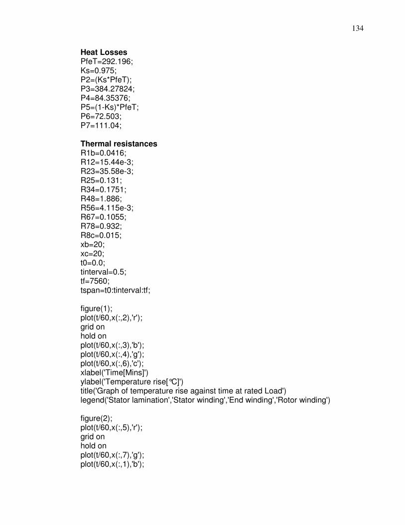
134
Heat Losses PfeT=292.196; Ks=0.975; P2=(Ks*PfeT); P3=384.27824; P4=84.35376; P5=(1-Ks)*PfeT; P6=72.503; P7=111.04; Thermal resistances R1b=0.0416; R12=15.44e-3; R23=35.58e-3; R25=0.131; R34=0.1751; R48=1.886; R56=4.115e-3; R67=0.1055; R78=0.932; R8c=0.015; xb=20; xc=20; t0=0.0; tinterval=0.5; tf=7560; tspan=t0:tinterval:tf; figure(1); plot(t/60,x(:,2),'r'); grid on hold on plot(t/60,x(:,3),'b'); plot(t/60,x(:,4),'g'); plot(t/60,x(:,6),'c'); xlabel('Time[Mins]') ylabel('Temperature rise[°C]') title('Graph of temperature rise against time at rated Load') legend('Stator lamination','Stator winding','End winding','Rotor winding') figure(2); plot(t/60,x(:,5),'r'); grid on hold on plot(t/60,x(:,7),'g'); plot(t/60,x(:,1),'b');

135
xlabel('Time[Mins]') ylabel('Temperature rise[°C]') title('Graph of temperature rise against time at rated load') legend('Rotor iron','End Ring','Frame') display('computed steady-state temperatures')
Program-B: Thermal network model for the squirrel cage induction machine
(11n), FULL SIM MODEL –Considered global R1b R12 R34 R25 C1 C2 C3 C4 P1 P2 P3 x0 t0 tf tspan xb xa xc R56 R23 global C8 C9 C10 C11 C12 R69 R910 R1011 R10a R311 R8c R48 R67 R78 global P4 P5 P6 P7 P8 P9 P10 P11 xc Thermal Differential equations Theta(1)=(1/C1)*(P1-(x(1)-xb)/R1b-(x(1)-x(2))/R12); Theta(2)=(1/C2)*(P2-(x(2)-x(1))/R12-(x(2)-x(3))/R23-(x(2)-x(5))/R25); Theta(3)=(1/C3)*(P3-(x(3)-x(2))/R23-(x(3)-x(4))/R34-(x(3)-x(11))/R311); Theta(4)=(1/C4)*(P4-(x(4)-x(8))/R48-(x(4)-x(3))/R34); Theta(5)=(1/C5)*(P5-(x(5)-x(2))/R25-(x(5)-x(6))/R56); Theta(6)=(1/C6)*(P6-(x(6)-x(7))/R67-(x(6)-x(5))/R56-(x(6)-x(9))/R69); Theta(7)=(1/C7)*(P7-(x(7)-x(8))/R78-(x(7)-x(6))/R67); Theta(8)=(1/C8)*(P8-(x(8)-x(4))/R48-(x(8)-x(7))/R78-(x(8)-xc)/R8c); Theta(9)=(1/C9)*(P9-(x(9)-x(6))/R69-(x(9)-x(10))/R910); Theta(10)=(1/C10)*(P10-(x(10)-x(9))/R910-(x(10)-x(11))/R1011-(x(10)-xa)/R10a); Theta(11)=(1/C11)*(P11-(x(11)-x(3))/R311-(x(11)-x(10))/R1011); global R1b R12 R34 R25 C1 C2 C3 C4 P1 P2 P3 R23 x0 t0 tf tspan xb xa xc global C5 C6 C7 C8 C9 C10 C11 C12 R69 R910 R1011 R10a R311 R8c R48 global P4 P5 P6 P7 P8 P9 P10 P11 xc Initial temperature x0=[20]; Thermal Capacitances C1=18446.55; C2=4450.625; C3=423.388; C4=539.92; C5=3204.08; C6=408.267; C7=218.785;

136
C8=1006; C9=C7; C10=C8; C11=C4; Heat Losses PfeT=292.196; Ks=0.975; P2=(Ks*PfeT); P3=384.27824; P4=84.35376; P5=(1-Ks)*PfeT; P6=72.503; P7=111.04; P9=P7; P11=P4 Thermal resistances R1b=0.0416; R12=15.44e-3; R23=35.58e-3; R25=0.131; R34=0.1751; R48=1.886; R56=4.115e-3; R67=0.1055; R78=0.932; R8c=0.015; R69=R67; R910=R78; R1011=R48; R10a=R8c; R311=R34; xb=20; xc=20; xa=20; t0=0.0; tinterval=0.5; tf=7560; tspan=t0:tinterval:tf; figure(1); plot(t/60,x(:,2),'r'); grid on hold on plot(t/60,x(:,3),'b');

137
plot(t/60,x(:,4),'g'); plot(t/60,x(:,6),'c'); xlabel('Time[Mins]') ylabel('Temperature rise[°C]') title('Graph of temperature rise against time at rated Load') legend('Stator lamination','Stator winding','End winding','Rotor winding') figure(2); plot(t/60,x(:,5),'r'); grid on hold on plot(t/60,x(:,7),'g'); plot(t/60,x(:,1),'b'); xlabel('Time[Mins]') ylabel('Temperature rise[°C]') title('Graph of temperature rise against time at rated load') legend('Rotor iron','End Ring','Frame') figure(3); plot(t/60,x(:,9),'r'); grid on hold on plot(t/60,x(:,11),'b'); xlabel('Time[Mins]') ylabel('Temperature rise[°C]') title('Graph of temperature rise against time at rated load') legend('End ringL','End windingL') display('computed steady-state temperatures')
Program-C: Thermal network model for the squirrel cage induction IM (13n), Half (LHS) of the LIM model --Considered
function Theta=oti3(t,x) global R1b R12 R34 R25 C1 C2 C3 C4 P1 P2 P3 x0 t0 tf tspan xb global C5 C6 C7 C8 R8c R48 R67 R78 R56 R23 global P4 P5 P6 P7 P8 xc Thermal Differential equations
138
Theta =zeros(8,1); Theta(1)=(1/C1)*(P1-(x(1)-xb)/R1b-(x(1)-x(2))/R12); Theta(2)=(1/C2)*(P2-(x(2)-x(1))/R12-(x(2)-x(3))/R23-(x(2)-x(5))/R25); Theta(3)=(1/C3)*(P3-(x(3)-x(2))/R23-(x(3)-x(4))/R34); Theta(4)=(1/C4)*(P4-(x(4)-x(8))/R48-(x(4)-x(3))/R34); Theta(5)=(1/C5)*(P5-(x(5)-x(2))/R25-(x(5)-x(6))/R56); Theta(6)=(1/C6)*(P6-(x(6)-x(7))/R67-(x(6)-x(5))/R56); Theta(7)=(1/C7)*(P7-(x(7)-x(8))/R78-(x(7)-x(6))/R67); Theta(8)=(1/C8)*(P8-(x(8)-x(4))/R48-(x(8)-x(7))/R78-(x(8)-xc)/R8c); global R1b R12 R34 R25 C1 C2 C3 C4 P1 P2 P3 x0 t0 tf tspan xb global C5 C6 C7 C8 R8c R48 R56 R78 R67 R23 global P4 P5 P6 P7 P8 xc Initial temperature x0=[20]; Thermal Capacitances C1=18446.55; C2=4450.625; C3=423.388; C4=539.92; C5=3204.08; C6=408.267; C7=218.785; C8=1006; Heat Losses PfeT=292.196; Ks=0.975; P2=(Ks*PfeT); P3=384.27824; P4=84.35376; P5=(1-Ks)*PfeT; P6=72.503; P7=111.04; Thermal resistances R1b=0.0416; R12=15.44e-3; R23=35.58e-3; R25=0.131; R34=0.1751; R48=1.886; R56=4.115e-3;

139
R67=0.1055; R78=0.932; R8c=0.015; xb=20; xc=20; t0=0.0; tinterval=0.5; tf=7560; tspan=t0:tinterval:tf; figure(1); plot(t/60,x(:,2),'r'); grid on hold on plot(t/60,x(:,3),'b'); plot(t/60,x(:,4),'g'); plot(t/60,x(:,6),'c'); xlabel('Time[Mins]') ylabel('Temperature rise[°C]') title('Graph of temperature rise against time at rated Load') legend('Stator lamination','Stator winding','End winding','Rotor winding') figure(2); plot(t/60,x(:,5),'r'); grid on hold on plot(t/60,x(:,7),'g'); plot(t/60,x(:,1),'b'); xlabel('Time[Mins]') ylabel('Temperature rise[°C]') title('Graph of temperature rise against time at rated load') legend('Rotor iron','End Ring','Frame') display('computed steady-state temperatures')
Program-D: Thermal network model for the squirrel cage induction IM (13n), Complete LIM model –Considered global R1b R12 R34 R25 C1 C2 C3 C4 P1 P2 P3 x0 t0 tf tspan xb xa xc global C8 C9 C10 C11 C12 R69 R910 R1011 R10a R311 R8c R48 R67 R78 global P4 P5 P6 P7 P8 P9 P10 P11 xc R56 R23

140
Thermal Differential equations Theta(1)=(1/C1)*(P1-(x(1)-xb)/R1b-(x(1)-x(2))/R12); Theta(2)=(1/C2)*(P2-(x(2)-x(1))/R12-(x(2)-x(3))/R23-(x(2)-x(5))/R25); Theta(3)=(1/C3)*(P3-(x(3)-x(2))/R23-(x(3)-x(4))/R34-(x(3)-x(11))/R311-(x(3)- x(12))/R312); Theta(4)=(1/C4)*(P4-(x(4)-x(8))/R48-(x(4)-x(3))/R34); Theta(5)=(1/C5)*(P5-(x(5)-x(2))/R25-(x(5)-x(6))/R56); Theta(6)=(1/C6)*(P6-(x(6)-x(7))/R67-(x(6)-x(5))/R56-(x(6)-x(9))/R69-(x(6)-x(13))/R613); Theta(7)=(1/C7)*(P7-(x(7)-x(8))/R78-(x(7)-x(6))/R67); Theta(8)=(1/C8)*(P8-(x(8)-x(4))/R48-(x(8)-x(7))/R78-(x(8)-xc)/R8c); Theta(9)=(1/C9)*(P9-(x(9)-x(6))/R69-(x(9)-x(10))/R910); Theta(10)=(1/C10)*(P10-(x(10)-x(9))/R910-(x(10)-x(11))/R1011-(x(10)-xa)/R10a); Theta(11)=(1/C11)*(P11-(x(11)-x(3))/R311-(x(11)-x(10))/R1011); Theta(12)=(1/C12)*(P12-(x(12)-x(3))/R312-(x(12)-x(13))/R1213); Theta(13)=(1/C13)*(P13-(x(13)-x(6))/R613-(x(13)-x(12))/R1213); global R1b R12 R34 R25 C1 C2 C3 C4 P1 P2 P3 x0 t0 tf tspan xb xa xc R613 R312 global C5 C6 C7 C8 C9 C10 C11 C12 C13 R69 R910 R1011 R10a R311 R8c global P4 P5 P6 P7 P8 P9 P10 P11 P12 P13 C13 R613 R312 R1213 P13 R56 Initial temperature x0=[20]; Thermal Capacitances C1=18446.55; C2=4450.625; C3=423.388; C4=539.92; C5=3204.08; C6=408.267; C7=218.785; C8=1006; C9=C7 C10=C8 C11=C4 C12=341.33 C13=871.566 Heat Losses PfeT=292.196; Ks=0.975; P2=(Ks*PfeT); P3=384.27824; P4=84.35376; P5=(1-Ks)*PfeT; P6=72.503; P7=111.04;

141
P9=P7 P11=P4 P12=68.113 P13=93.445 Thermal resistances R1b=0.0416; R12=15.44e-3; R23=35.58e-3; R25=0.131; R34=0.1751; R48=1.886; R56=4.115e-3; R67=0.1055; R78=0.932; R8c=0.015; R69=67 R910=R78 R1011=R48 R10a=R8c R311=R34 R613=0.002703 R312=0.02245 R1213=0.12576 xb=20; xc=20; xa=20; t0=0.0; tinterval=0.5; tf=7560; tspan=t0:tinterval:tf; figure(1); plot(t/60,x(:,2),'r'); grid on hold on plot(t/60,x(:,3),'b'); plot(t/60,x(:,4),'g'); plot(t/60,x(:,6),'c'); xlabel('Time[Mins]') ylabel('Temperature rise[°C]') title('Graph of temperature rise against time at rated Load') legend('Stator lamination','Stator winding','End winding','Rotor winding') figure(2); plot(t/60,x(:,5),'r');

142
grid on hold on plot(t/60,x(:,7),'g'); plot(t/60,x(:,1),'b'); xlabel('Time[Mins]') ylabel('Temperature rise[°C]') title('Graph of temperature rise against time at rated load') legend('Rotor iron','End Ring','Frame') figure(3); plot(t/60,x(:,9),'r'); grid on hold on plot(t/60,x(:,11),'b'); plot(t/60,x(:,12),'g'); plot(t/60,x(:,13),'c'); xlabel('Time[Mins]') ylabel('Temperature rise[°C]') title('Graph of temperature rise against time at rated load') legend('End ringR','End windingR','Stator teeth','Rotor teeth') display('computed steady-state temperatures')


![V'x(v,'V'xA)=j · 2020. 4. 28. · the equivalent motor circuit. Finite element analysis (FEA) in induction motors (1M) is a step towards the modern design of induction motors [15]](https://img.pdfslide.net/doc/110x75/5fc782d0c1220c0a070a382a/vxvvxaj-2020-4-28-the-equivalent-motor-circuit-finite-element-analysis.jpg)