Outcrop Prediction Problem 3: Using the Model Builder to Automate Outcrop Prediction

IntroductionThe “Model Builder” in ArcGIS offers a way to automate repetitive tasks that can be a significant time saver if you can master the technique. Basically you need to analyze your work flow systematically and then use the graphical tools in the model builder to build a visual “flowchart” of the work flow. Once the visual flowchart is built you can then “run” the model that will execute the steps in the flowchart. You can edit the model to use different inputs so once the model has been “debugged” you can apply it to any data set.

Model Builder FundamentalsThe Model Builder can be started from ArcMap or ArcCatalog from the standard toolbar as indicated in Figure 1. The ArcGIS system also has a very good help file section on using the Model Builder – just activate “Help > ArcGIS Desktop Help” and search for “ModelBuilder”. You build a model by “dragging & dropping” tools or data into the ModelBuilder window followed by connecting the data to the tools that operate on the data with the “connect” tool. You can edit the data symbols to point to different sources when operating on different data sets. The tools you insert into ModelBuilder can be chosen from the “ToolBox”, or can be custom tools created with ModelBuilder or Python. You can ultimately turn any model built with ModelBuilder into a custom tool that will prompt the user for proper input.

Starting FilesYou will need to download the following file to complete this exercise (download from the “Resources” section of the GIT461/561 USA online site):

OP_prob3_start.mdb

OP_prob3_start.idb.zip

Make sure that these files are in your project folder. You will need to use “7zip” to unzip the “OP_prob3_start.idb.zip” file to create the folder “OP_prob3_start.idb”. Make sure this folder is located in the same project folder as the “OP_prob3_start.mdb” file.

Alternatively, if you don’t have a USA online account you can access the starting file at the below web site:

http://www.usouthal.edu/geography/allison/gy461/gy461_project_resources.htm

Look for the “Outcrop Prediction” Heading in the list of projects.

Step 1: Define the Workflow into a FlowchartThe first step in ModelBuilder should be sketching out your workflow into a flowchart. For this project we will use the features from the geodatabase file “OP_prob3_start.mdb”. The goal will be to create a model that creates the final geologic map feature class starting with the topographic grid and the top and bottom contact grid as input into the model. Below is the workflow that you used in problems 1 and 2 :

1. Using the 3D grid math tool “minus” subtract the topographic grid from the bottom contact grid. This produces a new “Bot_Resid” grid. This tool object will be named “Minus_1”. The input data objects are named “bot_grd” and “ElevGrd”. Negative residual values indicate that strata above the bottom contact are exposed on the topographic surface. Positive values indicate that strata below the contact are exposed on the surface.

2. The minus tool will be used again to subtract the topographic grid from the top contact to produce a new “Top_Resid” grid. The tool object will be named “Minus_2”, and the input data objects ares “top_grd” and “ElevGrd”. Note that negative residual values represent places on the map where strata above the contact is exposed, whereas positive values represent locations where strata below the contact is exposed.

3. The “Bot_Resid” and “Top_Resid” grids will both be reclassified into “Bot_Reclass” and “Top_Reclass” respectively using the “Reclassify” tool. The reclassify tool objects will be named “Reclass_1” and “Reclass_2” respectively. The basis of the reclassification will be values <= to 0 will be assigned a “1”, while values > 0 will be assigned a “2”. This means that strata above the contact is assigned a “1”, whereas strata below the contact is assigned a “2”.

4. The “Top_Reclass” and “Bot_Reclass” are added together with the raster math tool “plus”. The tool object is named “Plus”, and the composite output grid is named “Reclass_Comp”. In this grid values of “2”, “3”, and “4” represent locations where the younger, intermediate, and older strata are exposed. The intermediate unit would then have “top” contact as its upper boundary, and the “bottom” contact at its base.

5. The raster grid “Reclass_Comp” is converted into a polygon feature class with the “Raster to Polygon” tool. The output feature class is put in the same geodatabase file that contains the starting grid files. The polygon feature class is named “Lithology”.

Step 2: Open Model Builder and Add Data and ToolsAt this time start ArcCatalog and click on the ModelBuilder tool in the standard toolbar. Also open the “Toolbox” so that you can “drag-and-drop” tools from the toolbox. In ArcCatalog expand the required folders so that you can see the data sources that you will be working with for this project. You should now see a blank model with tools and data accessible as in Figure 2.

Note that geodatabase file “OP_prob3_start.mdb” is an exact copy of the example problem from the outcrop prediction documentation up to the point just before the first grid subtraction operation. The rest of the manipulations will be automated by “ModelBuilder” to generate the final geologic map that is equivalent to the example exercise.

The first tool that is needed is the raster “minus” tool so “drag-and-drop” that tool on the ModelBuilder window. Next drag-and-drop the “Bot_grd” and “ElevGrid” from the ArcCatalog window into the ModelBuilder window. The minus tool should be a yellow color, and the data sources a blue color. Now use the connector tool to connect the “Bot_\Grdt” as the first parameter input into the “Minus” tool. Use the same method to connect the “ElevGrid” to the “Minus” tool as the second input parameter. The order is important so make sure the “Bot_Contact” is the first parameter. Rename the “Minus” tool to “Minus_1”, and then output of this tool to “Bot_Resid”.

Repeat the above process to create the “Top_Resid” grid naming the “Minus” tool as “Minus_2”. Your model should appear similar to Figure 3. Note that the output grids are colored green but may be used as input for other tools. You can right-click on any data or tool object with the “select” tool in the ModelBuilder window and then use “Rename” to change the object name in the window.

Step 3: Use the Reclassify Tool to Simplify the Residual GridsIn order for the residual grids to be useful they both need to be reclassified as described above. The “3D Analyst > Reclass Raster > Reclassify” tool will be used for this step. Any values less than or equal to 0.0 will be assigned a value of 1, and any residual values greater than 0.0 are assigned a value of 2. First connect the “Bottom_Resid” to the “Reclassify” tool, and then rename the tool and output grid to “Reclass_1” and “Bot_reclass” respectively. To set the reclassify levels select the “Reclass_1” with the select tool and then right-click on the highlighted tool. Choose “open” to open the settings dialog for the tool. Set the reclassify intervals as indicated in Figure 4. The lower limit of the first range, -10000, and the upper limit, +10000, needs to be of sufficient magnitude to incorporate all of the negative and positive values respectively. Use the same method to reclassify the top contact residual into “Top_Reclass”.

Step 4: Add the 2 Reclassified Rasters to Create a Composite RasterIn this step the 2 reclassed rasters are added together with the “Plus” raster tool. When this is processed the resulting composite raster follows the below rules:

Raster Value Geometry

2 Younger strata outcrops at surface

3 Intermediate strata outcrops at surface

4 Older strata outcrops at surface

At this time add the “Plus” tool and feed to it the “Top_Reclass” and “Bot_Reclass” rasters. The order does not matter. The output should be named “Reclass_Comp”. Your model should now look like Figure 5.

Step 5: Use “Raster to Polygon” to Create a Lithology Polygon Feature ClassThe raster composite can be viewed to display the shape of the geologic map, however, most geologists would prefer a true polygon feature class so that area and perimeter values for individual polygons could be easily extracted. The tool needed for this step is “Conversion Tools > From Raster > Raster to Polygon”. Add this tool to the ModelBuilder window and connect the “Reclass_Comp” as input into the tool. Highlight the “Raster to Polygon” tool and use “open” to set the destination for output to a polygon feature class named “Lithology” in the geodatabase file containing the original data (Figure 6). The Lithology polygon feature class will have the same attribute coding for the strata as the “Reclass_Comp” raster. The final appearance of the model should be very similar to Figure 7.

Step 6: Test the ModelTo test the model select “File > Run” from the ModelBuilder main menu. You will see a progress window pop up and then terminate when the model has completed. Inspect the “Lithology” polygon feature class in “OP_prob3_start.mdb” – it should match the polygon geometry of the map in Figure 8. This is also the example problem used in class to introduce the outcrop prediction method so it should be familiar to you.

Step 7: Make the Model a “General Purpose” ToolThe model may work just fine at this point but it can only operate on the same set of data sources. To really make the model useful we need to make it prompt the user for the input data – the top and bottom contacts and the topographic elevation grids – and the destination of the “Lithology” polygon feature class. Open the model in “ModelBuilder” by highlighting it in ArcCatalog and selecting “Edit”. For each of the input sources right-click on the data source and check “Model Parameter”. The letter “P” will appear next to the data source object when it is a model parameter. When the model is “run” by double clicking on the file a dialog box will pop up requesting the source of the model parameter. Proceed to make all of the starting data objects model parameters. Also make the final “Lithology” polygon feature class a model parameter.

If you try to execute the model at this time you will be prompted for the model parameters, however, the default sources will still be in the model. It would be better if the fields were blank. To make this happen right-click on the “Minus_1” tool object and select “Open”. Backspace over the “Input Raster” field until it is blank, and then select “OK”. You will notice that the connected data objects and tools now lose their color because there is no definitive data source linked to the tools. This is OK – when you execute the tool you will indicate the source in the dialog. Proceed to make the same changes to “Minus_2” and to the “Lithology” output object. The model should now appear like Figure 9. Now double-click on the model file in ArcCatalog. You should see an opening dialog like Figure 10. Note that if you want to re-order the parameter list in the dialog (Figure 10) you can do so by right-clicking

anywhere on the ModelBuilder window, and then select “Model Properties” and then the “Parameters” tab. You should also note that the output parameter “Lithology” may have a warning message next to it stating that “Lithology” will be overwritten. Most configurations of ArcGIS do not allow this to happen so you may have to rename the output polygon feature class to “Lithology2” or at least something different than “Lithology”. Note that sometimes this warning message will persist even if you delete “Lithology” from the geodatabase file.

Test the model on the Problem 2 USA campus data. Rename the existing “Lithology” polygon feature class to a different name before running the model so you can compare the results of the model to the original. The geometry should appear like Figure 11.

If you want your model to run without any file dependency make sure that any intermediate results produced by the tools are “blanked out”. For example in Figure 12 the “Minus_1” tool was highlighted and right-clicked on, and then “Open” was selected. The output raster field is blanked out, and that means that ArcGIS will make the intermediate raster result in a “scratch space” and then erase it when the model is finished executing. Blanking out these output fields removes any file dependency from the tool and makes your model more universally usable (Warning – do not get confused and “blank out” the input fields!). Proceed to “blank out” the output fields for all of the other tool objects (“Minus_2”, “Reclass_1”, etc.) in the model and then check to make sure the tool works as expected.

At this point file dependency is covered but there is still potentially a “loose end” to take care of if we want the model to be flexible. When the top and bottom residual grids were reclassified we chose a lower and upper limit of -99999 and +99999 that certainly works for the example data set but may not work correctly for another data set. The best scenario is to “expose” this criteria as a “variable” so that users of the model will see it and at least check it to see if it needs to be modified. Do this by highlighting the “Reclass_1” tool, right-clicking on it, and then select “Make Variable > From Parameter > Reclassification”. This will add a “blue” variable object to the model as depicted in Figure 13. Select the variable, right-click on it, and then set the reclassification ranges as indicated in Figure 13. Name this variable “Reclassification_1”. Do the same for “Reclass_2”.

To make the outcrop prediction tool accessible to ArcMap, open ArcMap at this time and load an outcrop prediction starting data set – in this case the data from “OPexample.mxd”. This file uses the data in “OPexample_start.mdb” so make sure it is available. Also open ArcCatalog and navigate to where you have created the new model tool in “MyToolbox.tbx”. Resize the ArcMap and ArcCatalog windows so you can see both. Open the “Toolbar” in ArcMap, and then “drag-and-drop” the toolbox icon (“Toolbox.tbx”) on the toolbar window in ArcMap. You should now see a new “MyToolbox” entry in the toolbox window. Expand it and double-click on the name of the model tool (“Outcrop Prediction Tool”) to begin running the tool. Enter the data from the example problem. The resulting geologic map in the feature class that you indicated as output will be added to the ArcMap project automatically. Figure 14 contains the modified toolbox with the example geologic map that has been symbolized.

Figure 1: A new blank model in Model Builder.

Figure 2: Blank model with tools and data accessible.

Figure 3: Starting the model with "minus" operations.

Figure 4: Setting the reclassify intervals for residuals.

Figure 5: Configuration of Model with "Plus" Tool Added.

Figure 6: Using the Raster to Polygon Tool.

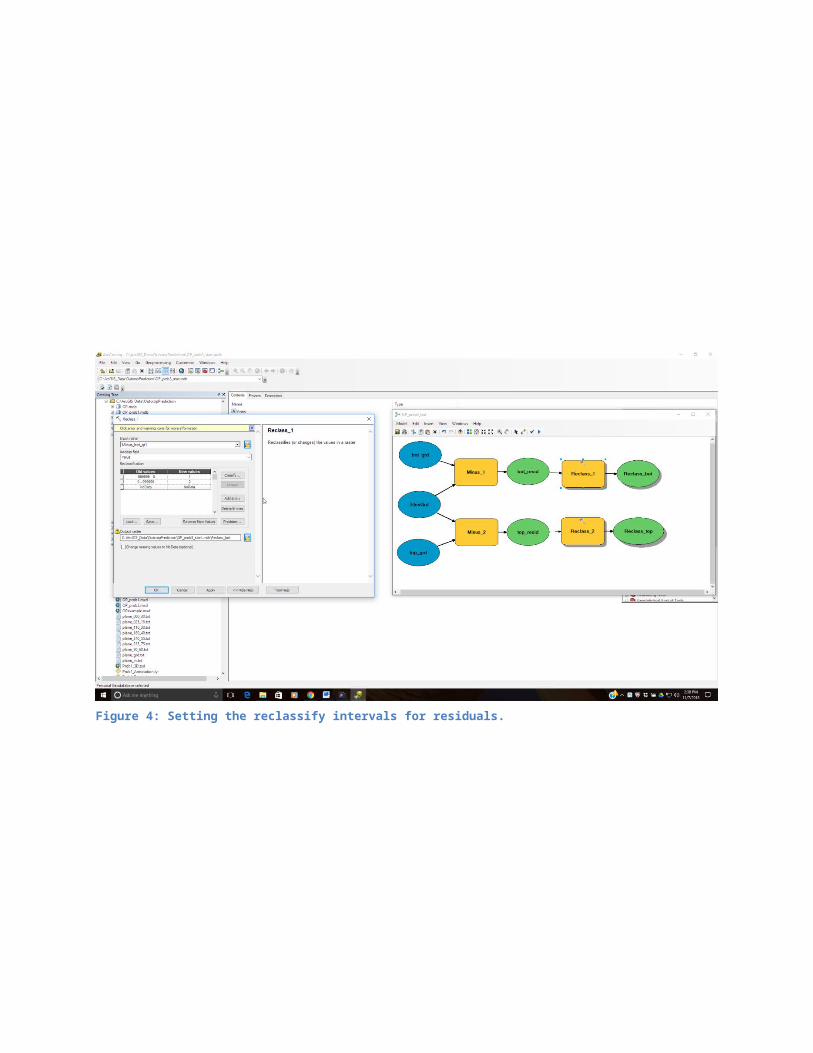
Figure 7: Final configuration of the Model.

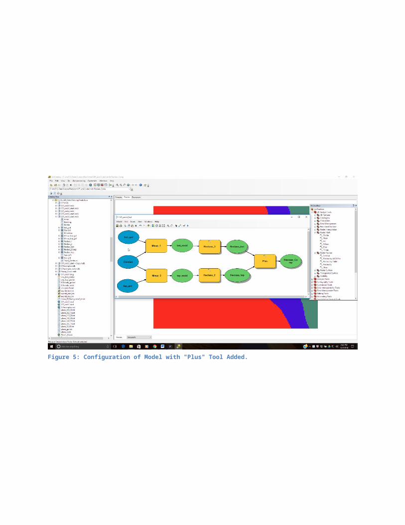
Figure 8: Correct “Lithology” geometry in "OP_prob3_start.mdb" geodatabase.

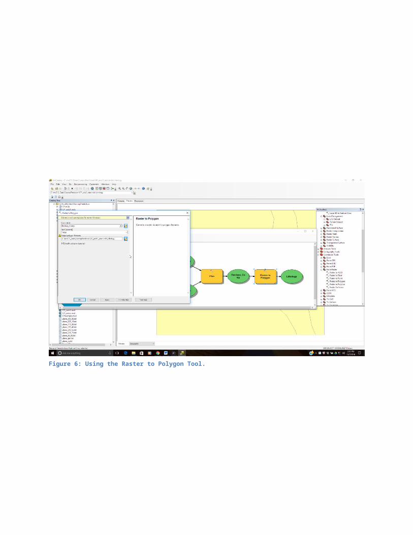
Figure 9: Model setup to use parameters for general purpose use.

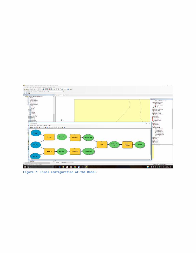
Figure 10: Appearance of the model using parameters.

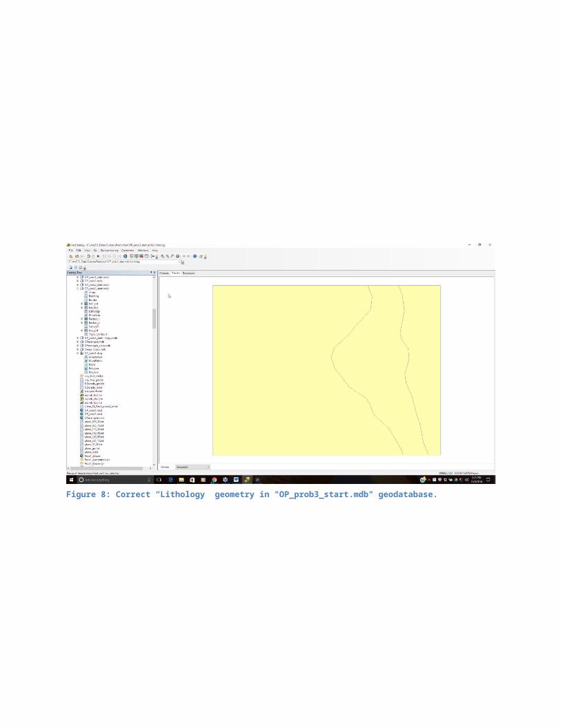
Figure 11: Problem 2 polygon feature class geometry produced with outcrop prediction model.

Figure 12: The parameter dialog listed for "Minus_1" tool with "Open" option.

Figure 13: Addition of a field definition variable to the “Reclass_2” tool object.

Figure 14: Results of outcrop prediction tool after executing on the example data set.