OUTDOOR RECREATION USE AND VALUE:

OUTDOOR RECREATION USE AND VALUE:SNAKE RIVER BASIN OF CENTRAL IDAHO

John R. McKeanAgricultural Enterprises, Inc.

R. G. TaylorUniversity of Idaho

Department of Agricultural Economics and Rural SociologyMoscow, Idaho 83844

Idaho Experiment Station Bulletin __-2000University of Idaho

Moscow, Idaho

ii

TABLE OF CONTENTS

TABLE OF CONTENTS . . . . . . . . . . . . . . . . . . . . . . . . . . . . . . . . . . . . . . . . . . . . . . . . . . . . . . . . ii

LIST OF FIGURES . . . . . . . . . . . . . . . . . . . . . . . . . . . . . . . . . . . . . . . . . . . . . . . . . . . . . . . . . . . iv

LIST OF TABLES . . . . . . . . . . . . . . . . . . . . . . . . . . . . . . . . . . . . . . . . . . . . . . . . . . . . . . . . . . . . iv

EXECUTIVE SUMMARY . . . . . . . . . . . . . . . . . . . . . . . . . . . . . . . . . . . . . . . . . . . . . . . . . . . . . . v

MEASUREMENT OF ECONOMIC VALUE . . . . . . . . . . . . . . . . . . . . . . . . . . . . . . . . . . . . . . 1Recreation Demand Methods . . . . . . . . . . . . . . . . . . . . . . . . . . . . . . . . . . . . . . . . . . . . . 4

Recreation Demand Survey . . . . . . . . . . . . . . . . . . . . . . . . . . . . . . . . . . . . . . . . . . . 4Travel Time Valuation . . . . . . . . . . . . . . . . . . . . . . . . . . . . . . . . . . . . . . . . . . . . . . . 7Disequilibrium Labor Market Model . . . . . . . . . . . . . . . . . . . . . . . . . . . . . . . . . . . . . 7

Disequilibrium and Equilibrium Labor Market Models . . . . . . . . . . . . . . 10Prices of Closely Related Goods . . . . . . . . . . . . . . . . . . . . . . . . . . . . . . . 12

Travel Cost Demand Variables . . . . . . . . . . . . . . . . . . . . . . . . . . . . . . . . . . . . . . . . 14Trip Prices - From Home to Site . . . . . . . . . . . . . . . . . . . . . . . . . . . . . . . 14Prices of Closely Related Goods . . . . . . . . . . . . . . . . . . . . . . . . . . . . . . . 14Other Exogenous Variables . . . . . . . . . . . . . . . . . . . . . . . . . . . . . . . . . . . 15

RECREATION DEMAND RESULTS . . . . . . . . . . . . . . . . . . . . . . . . . . . . . . . . . . . . . . . . . . . 15Estimated Demand Elasticities . . . . . . . . . . . . . . . . . . . . . . . . . . . . . . . . . . . . . . . . . . . . 15

Price Elasticity of Demand . . . . . . . . . . . . . . . . . . . . . . . . . . . . . . . . . . . 16Price Elasticity of Closely Related Goods . . . . . . . . . . . . . . . . . . . . . . . . 16Elasticity for Income and Time Constraints . . . . . . . . . . . . . . . . . . . . . . 16Elasticity With Respect to Other Variables . . . . . . . . . . . . . . . . . . . . . . . 17

Consumers Surplus per Trip . . . . . . . . . . . . . . . . . . . . . . . . . . . . . . . . . . . . . . . . . . . . . . 17Consumers Surplus Per Trip From Home to Site . . . . . . . . . . . . . . . . . . . . . . . . . . 17Total Annual Consumers Surplus for Outdoor Recreation . . . . . . . . . . . . . . . . . . . . 17

Comparison of Willingness-To-Pay With Other Studies . . . . . . . . . . . . . . . . . . . . . . . . 18

OUTDOOR RECREATION EXPENDITURES . . . . . . . . . . . . . . . . . . . . . . . . . . . . . . . . . . . 24Geographic Location of Recreation Economic Impacts . . . . . . . . . . . . . . . . . . . . . . . . 24Expenditure Per Visitor per Year and Total Annual Spending . . . . . . . . . . . . . . . . . . . 29Recreation Expenditure Rates by Town . . . . . . . . . . . . . . . . . . . . . . . . . . . . . . . . . . . . 29Recreation Lodging . . . . . . . . . . . . . . . . . . . . . . . . . . . . . . . . . . . . . . . . . . . . . . . . . . . . . 30

iII

Recreation Mode of Transportation . . . . . . . . . . . . . . . . . . . . . . . . . . . . . . . . . . . . . . . 30Importance of Recreation Activities During the Trip . . . . . . . . . . . . . . . . . . . . . . . . . . 31

REFERENCES . . . . . . . . . . . . . . . . . . . . . . . . . . . . . . . . . . . . . . . . . . . . . . . . . . . . . . . . . . . . . . . 33

APPENDIX I - Statistical concerns for demand curve estimation . . . . . . . . . . . . . . . . . . . . . . . . . . 41

APPENDIX II - QUESTIONNAIRES . . . . . . . . . . . . . . . . . . . . . . . . . . . . . . . . . . . . . . . . . . . . 43

Iv

LIST OF FIGURES

Figure 1 - Market demand for fishing . . . . . . . . . . . . . . . . . . . . . . . . . . . . . . . . . . . . . . . . . . . . . . . . 2Figure 2 - Recreation demand for an individual . . . . . . . . . . . . . . . . . . . . . . . . . . . . . . . . . . . . . . . . . 3Figure 3 - The three subregions . . . . . . . . . . . . . . . . . . . . . . . . . . . . . . . . . . . . . . . . . . . . . . . . . . . . 6Figure 5 - Travel cost versus recreation trips per year . . . . . . . . . . . . . . . . . . . . . . . . . . . . . . . . . . . 9Figure 6 - Travel time versus recreation trips per year . . . . . . . . . . . . . . . . . . . . . . . . . . . . . . . . . . 11

LIST OF TABLES

Table 1. Definition of variables . . . . . . . . . . . . . . . . . . . . . . . . . . . . . . . . . . . . . . . . . . . . . . . . . . . . 22Table 2 Snake River Basin recreation demand. . . . . . . . . . . . . . . . . . . . . . . . . . . . . . . . . . . . . . . . . 22Table 3. Effects of exogenous variables on recreation trips per year . . . . . . . . . . . . . . . . . . . . . . . . . 23Table 4 Anglers and recreationists by distance traveled . . . . . . . . . . . . . . . . . . . . . . . . . . . . . . . . . . 25Table 5 Spending by recreationists traveling to Central Idaho. . . . . . . . . . . . . . . . . . . . . . . . . . . . . . 26Table 6 Spending by recreationists while staying in Central Idaho . . . . . . . . . . . . . . . . . . . . . . . . . . 27Table 7 Spending by recreationists returning home from Central Idaho . . . . . . . . . . . . . . . . . . . . . . . 28Table 8 Overnight lodging by anglers. . . . . . . . . . . . . . . . . . . . . . . . . . . . . . . . . . . . . . . . . . . . . . . . 30Table 9 Type of transportation used by recreationists . . . . . . . . . . . . . . . . . . . . . . . . . . . . . . . . . . . 30Table 10 Importance of recreation activities during the outdoor recreation trip . . . . . . . . . . . . . . . . . 32

v

OUTDOOR RECREATION USE AND VALUE:SNAKE RIVER BASIN OF CENTRAL IDAHO

EXECUTIVE SUMMARYTwo surveys were conducted on recreationists in the Snake River Basin in central Idaho for the

purposes of: (1) measuring willingness-to-pay for recreation trips and, (2) measuring expenditures byrecreationists. The surveys were conducted by a single mailing using a list of names and addressescollected from recreationists in the Snake River Basin and surveys distributed by guides during April15, 1998 through November 30, 1998. The recreation demand survey resulted in 190 usableresponses. In comparison to the Lower Snake River Reservoir surveys and the Upstream of Lewistonsurveys, the central Idaho survey was hindered by a lack of central sites where recreationists could becontacted by clerks to obtain the names and addresses of those willing to participate in the survey. Theinclusion of a two dollar bill as an incentive payment also was not allowed for the central Idaho surveysbut was used in the prior surveys. One result was that a much larger share of the returned surveys wereincomplete. About 34 percent of the returned surveys were missing critical information and could notbe used for the demand analysis although they were useful to estimate averages. The response rate forthe travel cost questionnaire was not measurable because of the diverse methods used to distributesurveys.

The recreation demand analysis used a model that assumed persons did not (or could not) giveup earnings in exchange for more free time for outdoor recreation. This model requires extensive dataon recreationists’ time and money constraints, time and money spent traveling to the river recreationsites, and time and money spent during the recreation trip for a variety of possible activities. The travelcost demand model related recreation trips (from home to site) per year by groups of recreationists(average about 2.76 trips per year based on a sample of 190 anglers) to the dollar costs of the trip, tothe time costs of the trip, to the prices on substitute or complementary trip activities, and otherindependent variables. The dollar cost of the trip was based on reported travel distances from home tosite times the cost per person of 7.6 cents per mile.

The primary objective of the demand analysis was to estimate willingness-to-pay per trip forrecreation in the Snake River Basin in central Idaho. Consumer surplus (the amount by which totalconsumer willingness-to-pay exceeds the costs of production) was estimated at $87.24 per person pertravel cost trip. The average number of recreation trips per year from home to the Snake River Basin incentral Idaho was 2.76 (sample of 288 recreationists) resulting in an average annual willingness-to-payof $241 per year per recreationist. The total annual willingness-to-pay for all recreationists in theSnake River Basin of central Idaho is estimated at $25.1 million (see pages 31-32).

The recreation “demand” survey provided detailed information on samples of individuals whorecreated in the Snake River Basin in central Idaho. The information provided by these samples wasused to infer the spending behavior of recreationists in the Snake River Basin in central Idaho. Incapsule, the data collected by the demand survey provided information that was used to estimate the“willingness-to-pay” (marginal benefits) by consumers for various amounts of outdoor recreation.

vi

Estimation of the marginal benefits (demand) function allowed calculation of “net economic value” perrecreation trip.

The outdoor recreationist spending survey showed spending patterns useful in estimating thestimulus to jobs and business sales in the region created by recreationists attracted to the Snake RiverBasin in central Idaho. The surveys also provided information on transportation, lodging, and outdoorrecreation activities enjoyed by recreationists.

Research was funded by the Department of the Army, Corps of Engineers Walla WallaDistrict 201 North Third Avenue Walla Walla, Washington 99362 Contract No. DACW 68-96-D-003.

1 The competitive market equilibrium is economically “efficient” because total consumer benefits are maximized wheremarginal cost equals marginal benefits. If marginal costs exceed marginal benefits in a given market “rational”consumers will divert their spending to other markets.

1

MEASUREMENT OF ECONOMIC VALUE

A public good like the Snake River Basin differs in two significant ways from a competitivefirm. First, the public good is very large relative to the market that it serves; this is one of the reasonsthat a government agency is involved. Because of the size of the project, as output (recreation access)is restricted the price that people are willing to pay will increase (a movement up the market demandcurve). Price is no longer at a fixed level as faced by a small competitive firm. Second, the seller(government) does not act like a private firm which charges a profit-maximizing price. A public projecthas no equilibrium market price that can easily be observed to indicate value or, i.e., marginal benefit.

If output for recreation in the Snake River Basin in central Idaho was supplied by manycompetitive firms, market equilibrium would occur where the declining market demand curveintersected the rising market supply curve.1 A competitive market price would indicate the marginalbenefit to consumers of an added unit of outdoor recreation. However, calculation of total economicvalue produced would require knowledge of the market demand because many consumers would bewilling-to-pay more than the equilibrium price. The amount by which total consumer willingness-to-payexceeds the costs of production is the total net benefit or “consumers surplus.” If output was suppliedby many competitive firms, statistical estimation of a market demand curve could use observed marketquantities and prices over time.

Economic value (consumers surplus) of a particular output (outdoor recreation) of a publicgood also can be found by estimating the consumer demand curve for that output. The economic valueof recreation in the Snake River Basin in central Idaho can be determined if a statistical demandfunction showing consumer willingness-to-pay for various amounts of recreation is estimated. Becausemarket prices cannot be observed, (recreation is a non-market good), a surrogate price must be usedto model consumer behavior toward outdoor recreation (U.S. Army Corps of Engineers 1995;Herfindahl and Kneese 1974; McKean and Walsh 1986; Peterson et al. 1992).

The recreation demand survey collected information on individuals at the river showing theirnumber of recreation trips per year and their cost of traveling to the recreation site. The price faced byrecreationists is the cost of access to the recreation site (mainly the time and money costs of travel fromhome to site), and the quantity demanded per year is the number of recreation trips they make to theSnake River Basin. A demand relationship will show that fewer trips to the river are made by peoplewho face a larger travel cost to reach the river from their homes (Clawson and Knetsch 1966). “ TheTravel cost method (TCM) has been preferred by most economists, as it is based on observed marketbehavior of a cross-section of users in response to direct out-of-pocket and time cost of travel.”

2Travel cost models are incapable of predicting contingent behavior and involve current users. Another set ofeconomic models, contingent behavior and contingent value models, are typically used for projecting behavior ormeasuring non-use demand.

2

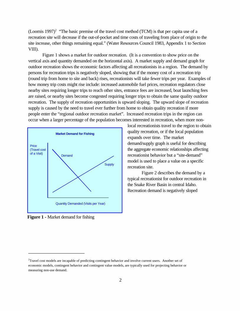
Market Demand for Fishing

Price(Travel costof a Visit)

Demand

Supply

Quantity Demanded (Visits per Year)

Figure 1 - Market demand for fishing

(Loomis 1997)2 “The basic premise of the travel cost method (TCM) is that per capita use of arecreation site will decrease if the out-of-pocket and time costs of traveling from place of origin to thesite increase, other things remaining equal.” (Water Resources Council 1983, Appendix 1 to SectionVIII).

Figure 1 shows a market for outdoor recreation. (It is a convention to show price on thevertical axis and quantity demanded on the horizontal axis). A market supply and demand graph foroutdoor recreation shows the economic factors affecting all recreationists in a region. The demand bypersons for recreation trips is negatively sloped, showing that if the money cost of a recreation trip(round trip from home to site and back) rises, recreationists will take fewer trips per year. Examples ofhow money trip costs might rise include: increased automobile fuel prices, recreation regulators closenearby sites requiring longer trips to reach other sites, entrance fees are increased, boat launching feesare raised, or nearby sites become congested requiring longer trips to obtain the same quality outdoorrecreation. The supply of recreation opportunities is upward sloping. The upward slope of recreationsupply is caused by the need to travel ever further from home to obtain quality recreation if morepeople enter the “regional outdoor recreation market”. Increased recreation trips in the region canoccur when a larger percentage of the population becomes interested in recreation, when more non-

local recreationists travel to the region to obtainquality recreation, or if the local populationexpands over time. The marketdemand/supply graph is useful for describingthe aggregate economic relationships affectingrecreationist behavior but a “site-demand”model is used to place a value on a specificrecreation site.

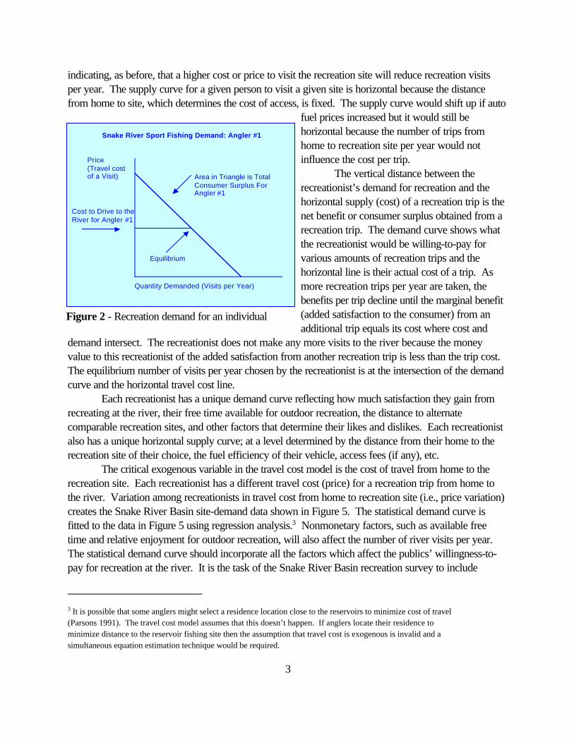
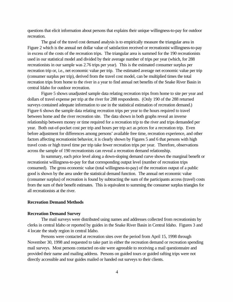
Figure 2 describes the demand by atypical recreationist for outdoor recreation inthe Snake River Basin in central Idaho. Recreation demand is negatively sloped

3 It is possible that some anglers might select a residence location close to the reservoirs to minimize cost of travel(Parsons 1991). The travel cost model assumes that this doesn’t happen. If anglers locate their residence tominimize distance to the reservoir fishing site then the assumption that travel cost is exogenous is invalid and asimultaneous equation estimation technique would be required.

3

Snake River Sport Fishing Demand: Angler #1

Price(Travel costof a Visit)

Quantity Demanded (Visits per Year)

Cost to Drive to theRiver for Angler #1

Equilibrium

Area in Triangle is TotalConsumer Surplus ForAngler #1

Figure 2 - Recreation demand for an individual

indicating, as before, that a higher cost or price to visit the recreation site will reduce recreation visitsper year. The supply curve for a given person to visit a given site is horizontal because the distancefrom home to site, which determines the cost of access, is fixed. The supply curve would shift up if auto

fuel prices increased but it would still behorizontal because the number of trips fromhome to recreation site per year would notinfluence the cost per trip.

The vertical distance between therecreationist’s demand for recreation and thehorizontal supply (cost) of a recreation trip is thenet benefit or consumer surplus obtained from arecreation trip. The demand curve shows whatthe recreationist would be willing-to-pay forvarious amounts of recreation trips and thehorizontal line is their actual cost of a trip. Asmore recreation trips per year are taken, thebenefits per trip decline until the marginal benefit(added satisfaction to the consumer) from anadditional trip equals its cost where cost and

demand intersect. The recreationist does not make any more visits to the river because the moneyvalue to this recreationist of the added satisfaction from another recreation trip is less than the trip cost. The equilibrium number of visits per year chosen by the recreationist is at the intersection of the demandcurve and the horizontal travel cost line.

Each recreationist has a unique demand curve reflecting how much satisfaction they gain fromrecreating at the river, their free time available for outdoor recreation, the distance to alternatecomparable recreation sites, and other factors that determine their likes and dislikes. Each recreationistalso has a unique horizontal supply curve; at a level determined by the distance from their home to therecreation site of their choice, the fuel efficiency of their vehicle, access fees (if any), etc.

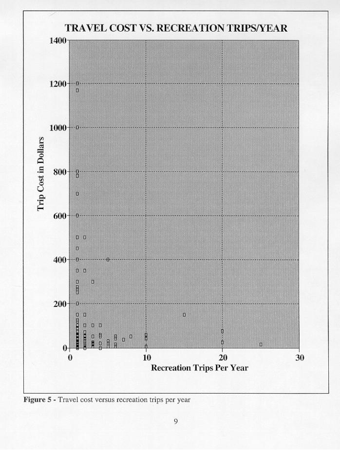
The critical exogenous variable in the travel cost model is the cost of travel from home to therecreation site. Each recreationist has a different travel cost (price) for a recreation trip from home tothe river. Variation among recreationists in travel cost from home to recreation site (i.e., price variation)creates the Snake River Basin site-demand data shown in Figure 5. The statistical demand curve isfitted to the data in Figure 5 using regression analysis.3 Nonmonetary factors, such as available freetime and relative enjoyment for outdoor recreation, will also affect the number of river visits per year. The statistical demand curve should incorporate all the factors which affect the publics’ willingness-to-pay for recreation at the river. It is the task of the Snake River Basin recreation survey to include

4

questions that elicit information about persons that explains their unique willingness-to-pay for outdoorrecreation.

The goal of the travel cost demand analysis is to empirically measure the triangular area inFigure 2 which is the annual net dollar value of satisfaction received or recreationist willingness-to-payin excess of the costs of the recreation trips. The triangular area is summed for the 190 recreationistsused in our statistical model and divided by their average number of trips per year (which, for 288recreationists in our sample was 2.76 trips per year). This is the estimated consumer surplus perrecreation trip or, i.e., net economic value per trip. The estimated average net economic value per trip(consumer surplus per trip), derived from the travel cost model, can be multiplied times the totalrecreation trips from home to the river in a year to find annual net benefits of the Snake River Basin incentral Idaho for outdoor recreation.

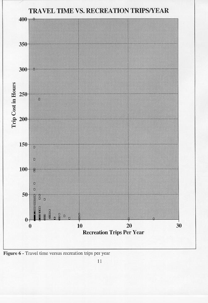
Figure 5 shows unadjusted sample data relating recreation trips from home to site per year anddollars of travel expense per trip at the river for 288 respondents. (Only 190 of the 288 returnedsurveys contained adequate information to use in the statistical estimation of recreation demand.) Figure 6 shows the sample data relating recreation trips per year to the hours required to travelbetween home and the river recreation site. The data shown in both graphs reveal an inverserelationship between money or time required for a recreation trip to the river and trips demanded peryear. Both out-of-pocket cost per trip and hours per trip act as prices for a recreation trip. Evenbefore adjustment for differences among persons’ available free time, recreation experience, and otherfactors affecting recreationist behavior, it is clearly shown by Figures 5 and 6 that persons with hightravel costs or high travel time per trip take fewer recreation trips per year. Therefore, observationsacross the sample of 190 recreationists can reveal a recreation demand relationship.

In summary, each price level along a down-sloping demand curve shows the marginal benefit orrecreationist willingness-to-pay for that corresponding output level (number of recreation tripsconsumed). The gross economic value (total willingness-to-pay) of the recreation output of a publicgood is shown by the area under the statistical demand function. The annual net economic value(consumer surplus) of recreation is found by subtracting the sum of the participants access (travel) costsfrom the sum of their benefit estimates. This is equivalent to summing the consumer surplus triangles forall recreationists at the river.

Recreation Demand Methods

Recreation Demand SurveyThe mail surveys were distributed using names and addresses collected from recreationists by

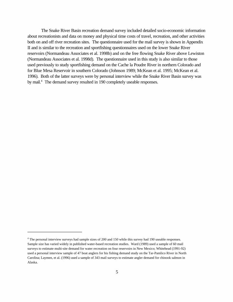
clerks in central Idaho or reported by guides in the Snake River Basin in Central Idaho. Figures 3 and4 locate the study region in central Idaho.

Persons were contacted at recreation sites over the period from April 15, 1998 throughNovember 30, 1998 and requested to take part in either the recreation demand or recreation spendingmail surveys. Most persons contacted on-site were agreeable to receiving a mail questionnaire andprovided their name and mailing address. Persons on guided tours or guided rafting trips were notdirectly accessible and tour guides mailed or handed out surveys to their clients.

4 The personal interview surveys had sample sizes of 200 and 150 while this survey had 190 useable responses. Sample size has varied widely in published water-based recreation studies. Ward (1989) used a sample of 60 mailsurveys to estimate multi-site demand for water recreation on four reservoirs in New Mexico; Whitehead (1991-92)used a personal interview sample of 47 boat anglers for his fishing demand study on the Tar-Pamlico River in NorthCarolina; Laymen, et al. (1996) used a sample of 343 mail surveys to estimate angler demand for chinook salmon inAlaska.

5

The Snake River Basin recreation demand survey included detailed socio-economic informationabout recreationists and data on money and physical time costs of travel, recreation, and other activitiesboth on and off river recreation sites. The questionnaire used for the mail survey is shown in AppendixII and is similar to the recreation and sportfishing questionnaires used on the lower Snake Riverreservoirs (Normandeau Associates et al. 1998b) and on the free flowing Snake River above Lewiston(Normandeau Associates et al. 1998d). The questionnaire used in this study is also similar to thoseused previously to study sportfishing demand on the Cache la Poudre River in northern Colorado andfor Blue Mesa Reservoir in southern Colorado (Johnson 1989; McKean et al. 1995; McKean et al.1996). Both of the latter surveys were by personal interview while the Snake River Basin survey wasby mail.4 The demand survey resulted in 190 completely useable responses.

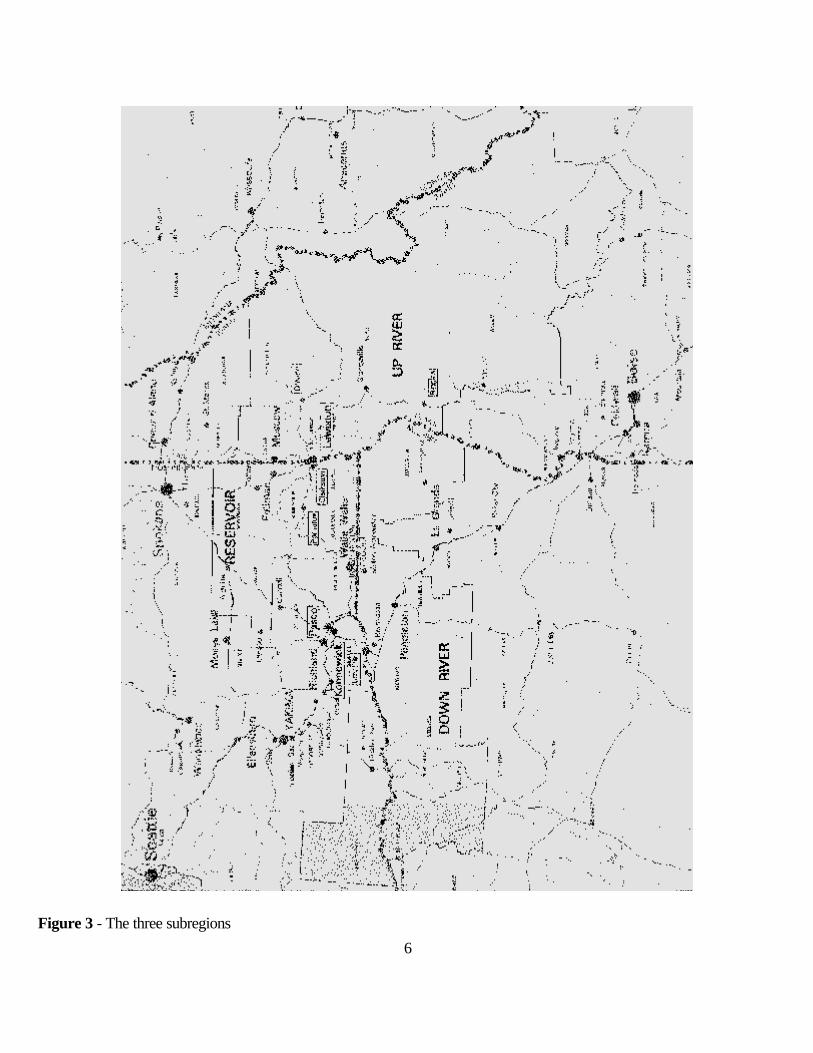
6Figure 3 - The three subregions

7

Travel Time ValuationThere has been disagreement among practitioners in the design of the travel cost model, thus

wide variations in estimated values have occurred (Parsons 1991). Researchers have come to realizethat nonmarket values measured by the traditional travel cost model are flawed. In most applications,the opportunity time cost of travel has been assumed to be a proportion of money income based on theequilibrium labor market assumption. Disagreements among practitioners have existed on the “correct”income proportion and thus wide variations in estimated values have occurred.

The conventional travel cost models assume labor market equilibrium (Becker 1965) so that theopportunity cost of time used in travel is given by the wage rate (see a following section). However,much dissatisfaction has been expressed over measurement and modeling of opportunity time values. McConnell and Strand (1981) conclude, "The opportunity cost of time is determined by an exceedinglycomplex array of institutional, social, and economic relationships, and yet its value is crucial in thechoice of the types and quantities of recreational experiences." The opportunity time valuemethodology has been criticized and modified by Bishop and Heberlein (1979), Wilman (1980),McConnell and Strand (1981), Ward (1983, 1984), Johnson (1983), Wilman and Pauls (1987),Bockstael et al. (1987), Walsh et al., (1989), Walsh et al. (1990a), Shaw (1992), Larson (1993), andMcKean et al. (1995, 1996).

The consensus is that the opportunity time cost component of travel cost has been its weakestpart, both empirically and theoretically. “Site values may vary fourfold, depending on the value oftime.” (Fletcher et al. 1990). “... the cost of travel time remains an empirical mystery.” (Randall 1994).

Disequilibrium in labor markets may render wage rates irrelevant as a measure of opportunitytime cost for many recreationists. For example, Bockstael et al. (1987) found a money/time tradeoff of$60/hour for individuals with fixed work hours and only $17/hour with flexible work hours.

The results from our previous studies and this study on the Snake River Basin in central Idahosuggest using a model specifically designed to help overcome disagreements and criticisms of theopportunity time value component of travel cost. We use a model that eliminates the difficult-to-measure marginal value of income from the time cost value. Instead of attempting to estimate a “moneyvalue of time” for each individual in the sample we simply enter the actual time required for travel to therecreation site as first suggested by Brown and Nawas (1973), and Gum and Martin (1975) andapplied by Ward (1983,1989). The annual income variable is retained as an income constraint. Anadded advantage of not using income to measure opportunity time value is that colinearity between thetime value component of travel cost and the income constraint should be greatly reduced.

Disequilibrium Labor Market ModelThe travel cost model used in this statistical analysis assumes that site visits are priced by both

(1) out-of-pocket travel expenses, and (2) opportunity time costs of travel to and from the site. Opportunity time cost has been conventionally defined in economic models as money income foregone(Becker 1965; Water Resources Council 1983). However, a person’s consideration of their limitedtime resources may outweigh money income foregone given labor market disequilibrium and institutionalconsiderations. Persons who actually could substitute time for money income at the margin represent asmall part of the population, especially the population of recreationists. Retirees, students, and

8

unemployed persons do not exchange time for income at the margin. Many workers are not allowedby their employment contracts to make this exchange. Weekends and paid vacations of prescribedlength are often the norm. Thus, the equilibrium labor market model may apply to certain self-employed persons, e.g., dentists or high level sales occupations, where individuals, (1) havediscretionary work schedules and, (2) can expect that their earnings will decline in proportion to thetime spent recreating. (Many professionals can take time off without foregoing any income). Theequilibrium labor market subgroup of the population is very small. According to U.S. Bureau of LaborStatistics and National Election Studies (U.S. Bureau of the Census 1993), only 5.4 percent of votingage persons in the U.S. were classified as self-employed in the United States in 1992. The labormarket equilibrium model applies to less than 5.4 percent of recreationists who are over-represented byretirees and students.

10

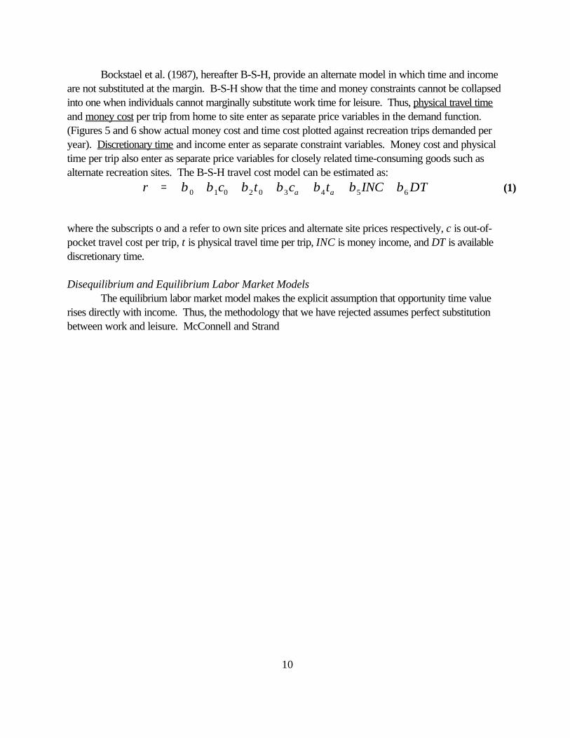
r c t c t INC DTa a= + + + + + +β β β β β β β0 1 0 2 0 3 4 5 6 (1)

Bockstael et al. (1987), hereafter B-S-H, provide an alternate model in which time and incomeare not substituted at the margin. B-S-H show that the time and money constraints cannot be collapsedinto one when individuals cannot marginally substitute work time for leisure. Thus, physical travel timeand money cost per trip from home to site enter as separate price variables in the demand function. (Figures 5 and 6 show actual money cost and time cost plotted against recreation trips demanded peryear). Discretionary time and income enter as separate constraint variables. Money cost and physicaltime per trip also enter as separate price variables for closely related time-consuming goods such asalternate recreation sites. The B-S-H travel cost model can be estimated as:

where the subscripts o and a refer to own site prices and alternate site prices respectively, c is out-of-pocket travel cost per trip, t is physical travel time per trip, INC is money income, and DT is availablediscretionary time.

Disequilibrium and Equilibrium Labor Market ModelsThe equilibrium labor market model makes the explicit assumption that opportunity time value

rises directly with income. Thus, the methodology that we have rejected assumes perfect substitutionbetween work and leisure. McConnell and Strand

5Although the equilibrium labor market model requires that the marginal effects of out-of-pocket cost and incomeforegone on quantity demanded be equal, empirical results often fail to support the model if the two components ofprice are entered separately in a regression.

12

( ) ( )[ ]r f c t g w= + ′ (2)

(1981, 1983) (M-S) specify price in their travel cost demand model as the argument in the right handside of equation two:

where, as before, r is trips from home to site per year, c is out-of-pocket costs per trip, and t is traveltime per trip. The term g'(w) is the marginal income foregone per unit time. It is assumed in the M-Smodel that any increase of travel cost, whether it is out-of-pocket spending or the money value of traveltime expended, has an equal marginal effect on visits per year. The term [c + (t)g'(w)] imposed thisrestriction because it forces the partial effect of a change in out-of-pocket cost (Mf/Mc) to be equal inmagnitude to a change in the opportunity time cost Mf/M[(t)g'(w)]. An important distinction in modelspecification is demonstrated by M-S. The equilibrium labor market model requires that out-of-pocketand opportunity time value costs be added together to force an identical coefficient on both costs.5 Incontrast, the B-S-H disequilibrium labor market model requires separate coefficients to be estimatedfor out-of-pocket costs and opportunity time value costs.

Measurement and statistical problems often beset the full price variable in empiricalapplications. Even for those self-employed persons who are in labor market equilibrium, measuringmarginal income is difficult. Simple income questions are unlikely to elicit true marginal opportunity timecost. Only after-tax earned income should be used when measuring opportunity time cost. Thus,opportunity cost may be overstated for the wealthy whose income may require little of their time. Conversely, students who are investing in education and have little market income will have their trueopportunity time costs understated. In practice, marginal income specified by theory is usually replacedwith a more easily observable measure consisting of average family income per unit time. Unfortunately, marginal and average values of income are unlikely to be the same.

Prices of Closely Related GoodsWard (1983,1984) proposed that the "correct" measure of price in the travel cost model is the

minimum expenditure required to travel from home to recreation site and return since any excess of thatamount is a purchase of other goods and is not a relevant part of the price of a trip to the site. Thisown-price definition suggests that the other (excess) spending during the trip is associated with some ofthe closely related goods whose prices are likely to be important in the demand specification. Forexample, time-on-site can be an important good and it is often ignored in the specification of the TCM. Yet time-on-site must be a closely related good since the weak complementarity principle upon whichmeasurement of benefits from the TCM is founded implies that time-on-site is essential. Weakcomplementary was the term used to connect enjoyment of a recreation site to the travel cost to reach it(Maler 1974). It is assumed that a travel cost must be paid in order to enjoy time spent at therecreation site. Without traveling to the site, the site has no recreation value to the consumer and

6 Bias in the consumer surplus estimate, created by exclusion of important closely related goods prices, depends onthe sign of the coefficient on the excluded variable, and the distribution of trip distances (McKean and Revier 1990). Exclusion of the price of a closely related good will bias the estimate of both the intercept and the demand slopeestimate (Kmenta 1971). Both these effects bias consumer surplus. Since the expression for consumer surplusgenerally is nonlinear, the expected consumer surplus is not properly measured by simply taking the area under thedemand curve. The distribution of trips along the demand function can affect the bias in consumers surplus,depending on the combination of intercept and slope bias created by the underspecification of the travel costdemand. Both intercept and slope biases and the trip distribution must be known in order to predict the effect ofexclusion of the price of a related good on the consumer surplus estimate.

13

without the ability to spend time at the site the consumer has no reason to pay for the travel. With theseassumptions, the cost of travel from home to site can be used as the price associated with a particularrecreation site (Loomis et al. 1986).

The sign of the coefficient relating trips demanded to particular time "expenditures" associatedwith the trip is an empirical question. For example, time-on-site or time used for other activities on thetrip have prices which include both the opportunity time cost of the individual and a charge against thefixed discretionary time budget. Spending more time-on-site could increase the value of the trip leadingto increased trips, but time-on-site could also be substituted for trips. Spending during a trip for goods,both on and off the site, consist of closely related goods which are expected to be complements fortrips to the site. Finally, spending for extra travel, either for its own sake, or to visit other sites, can be asubstitute or a complement to the site consumption. For example, persons might visit site "a" moreoften if site "b" could also be visited with a relatively small added time and/or money cost. If the priceof "b" rises, then visits to "a" might decrease since the trip to "a" now excludes "b". Conversely,persons might travel more often to "a" since it is now relatively less expensive compared to attaining "b"(McKean et al. 1996).

Many recreational trips combine sightseeing and the use of various capital and service itemswith both travel and the site visit, and include side trips (Walsh et al. 1990b). Recreation trips areseldom single-purpose and travel is sometimes pleasurable and sometimes not. The effect of these"other activities" on the trip-travel cost relationship can be statistically adjusted for through the inclusionof the relevant prices paid during travel or on-site and for side trips. Furthermore, both trips and on-site recreation are required to exist simultaneously to generate satisfaction or the weak complementarityconditions would be violated (McConnell 1992). A relation between trips and site experiences isindicated such that marginal satisfaction of a trip depends on the corresponding site experiences. Therefore, the demand relationship should contain site quality variables, time-on-site, and goods usedon-site, as well as other site conditions. Exclusion of these variables would violate the specificationrequired for the weak complementarity condition which allows use of the TCM to measure benefits.

In this study of outdoor recreation in the Snake River Basin, an expanded TCM survey wasdesigned to include money and time costs of on-site time (McConnell 1992), on-site purchases, and themoney and time cost of other activities on the trip. These vacation-enhancing closely related goodsprices are added to the specification of the conventional TCM demand model. Empirical estimates ofpartial equilibrium demand could suffer under-specification bias if the prices of closely related goodswere omitted.6 Traditional TCM demand models seemingly ignore this well known rule of

14

econometrics and exclude the prices of on-site time, purchases, and other trip activities which are likelyto be the principal closely related goods consumed by recreationists.

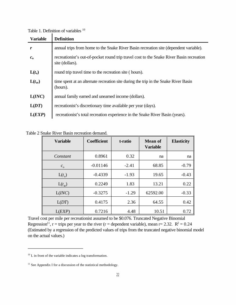
Travel Cost Demand VariablesThe definitions for the variables in the disequilibrium and equilibrium travel cost models are

shown in Table 1. The dependent variable for the travel cost model is (r), annual reported trips fromhome to the recreation site. Annual recreation trips from home to the Snake River Basin recreation siteis the quantity demanded. The average recreationist took 2.76 trips from home to the recreation site inthe Snake River Basin during the period April 15, 1998 - November 30, 1998.

Trip Prices - From Home to SiteThe money price variable in the B-S-H model is cr, which is the out-of-pocket travel costs to

the recreation site. Our mail survey obtained travel costs for most of those surveyed. Reported one-way travel distance for each party was multiplied times two and times $0.076 to obtain money cost oftravel per person per trip. Cost per mile was based on average cost collected from the much largerLower Snake River Reservoirs survey. Recreationist-perceived cost was used rather than costsconstructed from Department of Transportation or American Automobile Association data. Recreationists’ perceived price is the relevant variable when they decide how many recreation trips totake (Donnelly et al. 1985). Money price of a trip had the expected negative sign in the estimatedmodel.

The physical time price for each individual in the B-S-H model (disequilibrium labor market) ismeasured by to which is round trip driving time in hours. Average round trip driving time was about19.65 hours with an average round trip distance of 905.88 miles. Thus, average speed was 46.1 milesper hour. The time price of a trip had the expected negative sign in the estimated model.

Prices of Closely Related Goods The B-S-H model calls for the inclusion of ta, round trip driving time from home to an alternate

recreation site, as the physical time price of an alternate recreation site. This variable was not significantand appeared to be highly correlated with the monetary cost of travel. Another alternate site pricevariable is ca, which is the out-of-pocket travel costs to the most preferred alternate recreation site fromthe recreationists home. This substitute price variable also was not significant.

The variable to measure available free time is DT. The discretionary time constraint variable isrequired for persons in a disequilibrium labor market who cannot substitute time for income at themargin. Restrictions on free time are likely to reduce the number of recreation trips taken. Thediscretionary time variable has been positive and highly significant in previous disequilibrium labormarket recreation demand studies and was highly significant in this study (Bockstael et al. 1987;McKean et al. 1995, 1996). The average number of days that persons in the survey were “free fromother obligations” was 65 days per year.

The income constraint variable (INC) is defined as average annual family income resulting fromwage earnings. The relation of quantity demanded to income indicates differences in tastes amongincome groups. Although restrictions on income should reduce overall purchases, it may also cause ashift to low cost types of consumer goods such as outdoor recreation. Thus, the sign on the incomecoefficient conceptually can be either positive or negative. The estimated coefficient on income was

15

negative for this data set.Four other closely related goods prices were tested in the model: tos, time spent at the primary

recreation site at the river, cos money purchases at the primary recreation site at the river, cas, moneyspent during the trip at alternate recreation sites in central Idaho during the recreation trip, andrecreation time spent at an alternate recreation site in central Idaho during the trip , tar. Only the lattervariable was significant in this data set. The larger the amount of alternate site time during the trip, thegreater the number of trips taken.

Other Exogenous VariablesAn indicator of taste related particularly to the study region is the number of years that the

recreationist has visited the Snake River basin in central Idaho. The variable EXP measures this aspectof taste. Recreationists had an average of 10.5 years experience visiting the Snake River Basin. Theestimated coefficient on EXP was significant and had the expected positive sign.

Age has often been found to influence the demand for various types of recreation activity. Theaverage age of persons in the survey was 40.2 years. Age of the recreationist was tested in thestatistical demand model and found non-significant.

RECREATION DEMAND RESULTS

The t-ratios for all important variables to estimate the value of outdoor recreation arestatistically significant from zero at the 5 percent level of significance or better. The tests foroverdispersion (Cameron and Trivedi 1990; Greene 1992) for the Poisson regression were negative. Thus, unlike the data sets for the Lower Snake River Reservoirs and upstream of Lewiston, Poissonregression was appropriate. However, truncated negative binomial regression is reported. Aconservative approach uses the negative binomial model to eliminate any possible overstatement of thet-ratios that might occur with the Poisson regression. In fact, the t-ratios were somewhat higher for thePoisson regression (not shown) than for the negative binomial regression.

Estimated Demand Elasticities

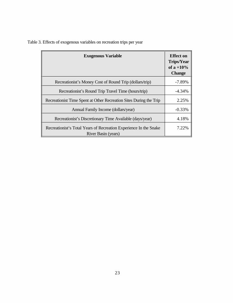
The estimated regression coefficients and elasticities from the truncated negative binomialregression estimation for the Snake River Basin recreation demand models are reported in Tables 2 and3. Elasticity refers to the percentage change in the dependent variable (trips) caused by a one percentchange in the independent variable (unless otherwise noted). Several of the exogenous variables in thetruncated negative binomial regressions were log transforms. When the independent variables are logtransforms the estimated slope coefficients directly reveal the elasticities. When the independent

7 Let the regression equation be ln(r) = "1 + "2 D + "3 ln(Z) where Z represents all the continuous independentvariables. The equation can be written as r = e ("1 + "2D) Z("3). Elasticity of r with respect to D is defined as , = (%change in r) / (% change in D) = (Mr/MD)(D/r). Mr/MD ="2 e ("1 + "2D) Z("3) ; D can be 0, 1, or E(D); and r is definedabove. Elasticity reduces to , = "2D. Thus, , becomes zero if D is zero and , takes the value "2 if D is one.

16

variables are linear the elasticities are found by multiplying the coefficient times the mean of theindependent variable. Elasticity with respect to dummy variables could be estimated for at least threesituations, the dummy variable is zero, the dummy variable is one, or the average value of the dummyvariable. Given a log transform of the dependent variable, elasticity for a dummy variable is zero if thedummy is zero, the estimated slope coefficient if the dummy is one, and the slope coefficient times theE(dummy) if the average value of the dummy is used. We will report the elasticity for the case wherethe dummy is one.7

Price Elasticity of DemandPrice elasticity with respect to out-of-pocket travel cost is -0.7891. A ten percent increase in

travel costs would reduce participation by 7.89 percent.The elasticity with respect to physical travel time for recreationists was -0.4339. If the time

cost of travel required to reach the site increased by ten percent, trips would decrease by 4.34 percent.

Price Elasticity of Closely Related Goods Time spent during the trip at alternate recreation sites in the Snake River basin, tar, has a price

elasticity of 0.2249. Thus, increases in the amount of time spent at alternative recreation sites during thetrip tends to increase the number of trips. The time spent at an alternate site acts as a complementarygood to the overall recreation trip experience in central Idaho. Since both the primary site and thealternate site are in the Snake River Basin, it is desired to include both contributions to recreationdemand.

Elasticity for Income and Time ConstraintsIncome elasticity was weakly significant for this data set. Quantity demanded (recreation trips

from home to the Snake River per year) was lower for high income persons. The elasticity of -0.3275indicates that a person with a ten percent higher income level will take 3.28 percent less trips. It is notunusual to find that outdoor recreation is negatively related to income.

Elasticity with respect to discretionary time is 0.4175. As in past studies, the discretionary timevariable was positive and highly significant. A ten percent increase in free time results in a very large4.18 percent increase in recreation trips to the Snake River Basin. As expected, available free timeacts as an important constraint on the number of recreation trips taken per year.

Elasticity With Respect to Other VariablesThe recreation experience variable, EXP, was highly significant. The coefficient showed that

those who have recreated in the Snake River Basin over a long period of time tend to make more trips

8 This assumes that anglers in the Snake River Basin and anglers on the four reservoirs on the Lower Snake Riveruse vehicles having similar fuel efficiency. Money travel cost per mile for a vehicle is based on the much largersample (537 observations versus 190 observations) collected for the reservoirs.

17

to the area. A ten percent increase in years visited the river results in a very large 7.22 percent increasein annual trips to the river.

Consumers Surplus per TripConsumers’ surplus was estimated using the result shown in Hellerstein and Mendelsohn

(1993) for consumer utility (satisfaction) maximization subject to an income constraint, and where tripsare a nonnegative integer. They show that the conventional formula to find consumer surplus for asemilog model also holds for the case of the integer constrained quantity demanded variable. ThePoisson and negative binomial regressions, with a linear relation on the explanatory own monetary pricevariable are equivalent to a semilog functional form. Adamowicz et al. (1989) show that the annualconsumers surplus estimate for demand with continuous variables is E(r)/(-ß), where ß is the estimatedslope on price and E(r) is average annual visits. Consumers surplus per trip from home to site is 1/(-ß). (Also note that the estimate of consumers surplus is invariant to the distribution of trips along thedemand curve when surplus is a linear function of Q. Thus, it is not necessary to numerically calculatesurplus for each data point and sum as would be the case if the surplus function was nonlinear.)

Consumers Surplus Per Trip From Home to Site Estimated coefficients for the travel cost model with labor market disequilibrium, and assuming

travel cost per mile of 7.6 cents per mile per person are shown in Table 2. The assumption of 7.6 centsper mile per person is identical with that used in the fishing and recreation demand models estimated forthe four reservoirs on the Lower Snake River (Normandeau Associates et al. 1998b) and on the FreeFlowing Snake River above Lewiston (Normandeau Associates et al. 1998d).8

Application of truncated negative binomial regression, and using recreationist-reported traveldistance times $0.076 per mile per person to estimate out-of-pocket travel costs, results in an estimatedcoefficient of -0.011462 on out-of-pocket travel cost. Consumers surplus per recreationist per trip isthe reciprocal or $87.24. Average recreationist trips per year in our full 288-person sample was 2.76. Total surplus per recreationist per year is average annual trips x surplus per trip or 2.76 x $87.24 =$241 per year. Total Annual Consumers Surplus for Outdoor Recreation

An important objective of the demand analysis was to estimate total annual willingness-to-payfor recreation in the Snake River Basin. As discussed above, consumer surplus was estimated at$87.24 per person per travel cost trip. The average number of recreation trips per year from home tothe Snake River Basin was 2.76 resulting in an average annual willingness-to-pay of $241 per year perrecreationist. The annual recreation value of the Snake River Basin for our sample of recreationists orwillingness-to-pay by those in our sample of 190 recreationists is 190 x $241 = $45,790 per year.

The total annual willingness-to-pay for all recreationists requires knowledge of the total

18

population of recreationists which frequent the Snake River Basin. The number of nonanglerrecreationists visiting central Idaho was estimated to be 180,000 per year. The number ofrecreationists was derived from data collected in the spending survey and published information ontraveler spending for the States of Idaho and Oregon. The detailed derivation is shown in the secondsection (the input-output spending survey) of this report. Total annual consumer surplus for nonanglingrecreationists in central Idaho is estimated to be 180,000 x $241 = $43.4 million per year.

Comparison of Willingness-To-Pay With Other StudiesComparisons of net benefits for outdoor recreation among demand studies is difficult because

of differences in the units of measurement of consumption or output. Comparisons of value per persontrip are flawed unless all studies compared have similar length of stays. Comparisons of value perperson per day are difficult because some sites and activities can occur all day (or even at night) andothers only at certain hours. Conversion problems for recreation consumption data makes exactcomparison among studies impossible. Many studies are quite old and the purchasing power of thedollar has declined over time. Adjustment of values found in older studies to current purchasing powercan be attempted using the consumer price index. Another problem with older studies is the changes inboth economic and statistical models used to measure value. Adjustment for different travel cost modelmethodologies, as well as contingent value methodologies, and inflation, is shown in Walsh et al.(1988a; 1988b; 1990a). Some of the more recent studies used higher cost per mile than we did fortravel and also used income rate as opportunity time cost that was added to the monetary costs oftravel. If these outmoded methods resulted in an overstatement of travel cost, a near proportionaloverstatement of estimated consumer surplus will occur. In addition, some of the studies used Poissonregression and obtained extremely large t-values. Although no test for overdispersion was mentioned,the very high t-values suggest that the requirement of Poisson regression that the mean and variance oftrips per year be equal was violated. If that is the case, the Poisson regressions are inappropriate andshould have been replaced with negative binomial regression.

Cameron et al. (1996) developed individual travel cost recreation models to predict the effectof water levels on all types of recreation at reservoirs and rivers in the Columbia River Basin. SeeAppendix J-1, COE Columbia River System Operation Review (CRSOR) (1995). The baseline(1993 water levels) estimates of consumer surplus varied between $13 and $99 per person per summermonth over the nine sites. Annual estimates per trip were not reported. The study included recreationat Lower Granite Reservoir with a sample of 168 persons. The results for Lower Granite Reservoirwere extrapolated to the other three Lower Snake River reservoirs. Consumer surplus per recreationday for summer recreation can be found using average visitor days shown in Tables 6,2g-6,2j and totalsummer consumer surplus shown in Tables 6,3g-6,3j (CRSOR). Division of total consumer surplus byaverage recreation days result in: Ice Harbor Reservoir $51.21 per recreation day, Lower MonumentalReservoir $40.33 per recreation day, Little Goose Reservoir $42.69 per recreation day, and LowerGranite Reservoir $35.40 per recreation day. Recreation days varied from 138,400 at LowerMonumental Reservoir to 1,670,600 at Lower Granite Reservoir. Values found for other reservoirs inthe study included John Day Reservoir at $20.14 per recreation day, Lake Roosevelt Reservoir at

9 About 12.5 percent of recreationists in this sample indicated they gave up some income to travel to the recreationsite. Our prior survey of anglers resulted in 11.9 percent indicating they gave up some income to travel to thefishing site.

19

$53.27 per recreation day, and Dworshak Reservoir at $54.01 per recreation day. The values found in CRSOR (Cameron et al. 1996) are higher than estimated herein. Changes

in consumer surplus estimated by the travel cost method are almost directly proportional to the changesin travel cost value that is used as price in the demand function. One reason for the high values in theCRSOR study is that the vehicle cost used in the price variable was $0.29 cents per mile (Departmentof Transportation estimate) whereas our vehicle cost was $0.202 per mile (based on our survey data). The price perceived by travelers is the appropriate measure. DOT data include fixed costs that are notrelevant when making incremental trip decisions (Donnelly et al. 1985). In addition, Cameron et al.1996, added in an opportunity time cost of travel based on estimated travel time valued at the reportedaverage wage rate (see CRSOR, Appendix J-1, bottom of Table 5,4). Our methodology did notinclude a money cost of time in travel cost and physical travel time was included as a separate site pricevariable. Their assumption that all recreationists give up earnings when traveling to the site is incorrectbased on their own survey data. The fraction of persons who stated they gave up some income to visitthe sites appears to be only about 10 percent (about 19 persons) in their sample of 186 at LowerGranite Reservoir (see CRSOR, Cameron et al. 1996, Appendix B2 Survey Results part E, AboutYour Typical Trips).9 The ten percent of visitors that gave up some income probably did so either onthe way to the site or on the return trip but not both ways. The appropriate foregone income amountwould only apply to half the trip time and to only ten percent of the visitors. Based on the surveycharacteristics of typical trips, the foregone income component of travel cost was overstated by about95 percent. Their travel cost measure also included lodging costs which are discretionary and are notusually considered part of the cost of a recreation trip (CRSOR, Appendix C). Their average “roundtrip transportation cost” to travel to the Lower Snake River reservoirs was about $23.37 per trip perperson whereas ours was about $9.93 per trip per person.

English and Bowker (1996) estimated travel zonal cost models for outfitted rafting on theChattooga River which forms the border between Georgia and South Carolina. The mail surveyresulted in 331 useable responses which was reduced to 214 observations when organized groupswere removed. They experimented with several definitions of travel cost, all of which excludedforegone income. If travel cost was assumed to be $0.15 per mile, the consumer surplus per trip was$31.66. At the other extreme, if all outfitter costs, transportation, lodging, activities, and food costswere included as part of the travel cost then consumer surplus increased to $104.64 per trip.

Bowker, et al (1996) reported on two individual observation travel cost models which usedtruncated negative binomial regression. The study was on commercial guided rafting on the Chatoogaand Nantahala rivers in Georgia, South Carolina and in North Carolina. The mail surveys resulted in369 and 376 useable responses respectively. They conclude that $0.092 per mile per person is in linewith reported variable travel expenses and caution against the very high values used in some studies. Consumer surplus estimated are presented for various level of assumed foregone income and forreported cost versus a fixed cost per mile. With no foregone income and imputed cost of 9.2 cents per

20

$89.03 on the Nantahala River. The estimates of consumer surplus per person per trip can rise as highas $286 dollars when it is assumed that 50 percent of the wage rate is foregone during the trip.

Michaleson (1977) used the individual observation travel cost method to estimate the value ofcamping associated with wild and scenic river recreation in Idaho. The imputed value of time wasincluded in travel cost. He reported a value of $9 per activity day in 1971 dollars. Michaleson andGilmour (1978) estimated the value of outdoor recreation trips associated with camping. An imputedvalue of time was included in travel cost. The study method was individual observation travel cost andused on site interviews in Sawtooth Valley, Idaho. The average value was $3.73 per person per day in1971 dollars.

Brown and Plummer (1979) used the hedonic travel cost method to find the value ofcamping in western Washington. The imputed value of time was excluded from travel cost. They founda value for camping of $5.83 per person per day in 1976 dollars.

Sutherland (1980) used the zonal travel cost method to estimate the values of camping,swimming, and motorized boating in Idaho, Oregon and Washington states. The imputed value oftravel time was excluded from travel costs. Values of $4.23 per person per day for camping, $4.31per person per day for swimming, and $4.24 per person per day for motorized boating (all in 1979dollars) were found.

Findeis and Michalson (1984) used a modified individual observation travel cost method toestimate the value of camping at developed sites in the Targhee National Forest in Idaho. An imputedvalue of time was included in travel cost. They found a value of $8.60 to $17.93 per person per day in1974 dollars.

Daniels (1987) applied a zonal travel cost model in a study of visitors to four campgrounds inLolo National Forest in Montana. An imputed value of time was included in travel cost. One-third ofthe sample were nonresidents and were all deleted on the grounds that the campgrounds were not theirprimary destination. An average value of $17.82 per person per day was found (in 1984 dollars).

Brox and Kumar (1997) apply a multi-site travel cost model for camping at 48 provincial parksin Ontario, Canada. The imputed value of time was excluded from travel cost but the arbitrary(government reimbursement rate) value for travel cost per mile was overstated. They report values pertrip varying by park from $1.80 to $7,000 with most values under $300 per trip in 1990 dollars.

Knetch et al. (1976) used a zonal travel cost model to estimate the demand for day trips toCalifornia reservoirs where picnicking made up a large part of the activities. Truncation to day use onlyreduced the values significantly. An imputed value of time was included in travel cost. They found avalue of $3.33 in 1969 dollars.

Walsh et al. (1980) measured the value of camping, picnicking and fishing on high countryreservoirs located along the eastern slopes of the Rocky Mountains in Colorado. They usednoniterative open-ended contingent value questions in on site interviews. They found a value of $10.90per person per day in 1978 dollars.

Walsh and Olienyk (1981) applied an iterative contingent value survey on site to valuepicnicking at five recreation sites in national forests on the eastern slopes of the Rocky Mountains inColorado. They found a value of $6.22 per person per day in 1980 dollars.

Ward (1982) estimated the demand for recreation (picnicking, boating, swimming) at reservoirs

21

in southeastern new Mexico. He used an individual observation travel cost for model. An imputedvalue of time was included in travel cost. The survey was truncated to neighboring counties whichwould understate value. He found a value of $11.39 per person per day in 1978 dollars.

Rosenthal (1987) applied a zonal travel cost model to study recreation demand at 11 reservoirsin Kansas and Missouri. Recreation activities included picnicking, swimming, fishing and boating. Thesample was limited to one-day trips which would understate value. An imputed value of time wasincluded in travel cost. He found values of $4.04 to $7.10 per person per day in 1982 dollarsdepending upon treatment of substitute sites.

Wade et al. (1988) used a zonal travel cost model to find the demand for swimming at 14reservoirs in California. An imputed value for time was included in travel cost. The estimated value per person per day ranged from $15.84 to $35.04 in 1985 dollars. They alsoestimated the value of motorized boating on Lake Havasu in Arizona and at 12 reservoirs in California. An imputed value of time was included in travel cost. They found a value at Lake Havasu of $34.64per day in 1985 dollars. Lake Havasu is unique for a number of reasons including reconstruction of theoriginal London Bridge. Motorized boating at the California reservoirs was double in southernCalifornia compared with reservoirs in the rest of the state. The average value for motorized boating onreservoirs in California was $24.28 per person per day in 1985 dollars.

Brooks (1988) used a travel cost model to estimate the value of deer hunting in Montana. Animputed value of time was included in travel cost. The sample included both resident and nonresidenthunters. Average value per person per day varied from $20.88 to $54.94 in 1986 dollars.

Offenbach and Goodwin (1994) estimate the demand for deer hunting in Kansas. They use anindividual observation travel cost model estimated using the negative binomial regression technique. Animputed value of time was excluded from travel cost but costs for food and lodging were added totransport costs. They found value per trip of $160.79 to $176.55 in 1988 dollars. Data were notreported allowing conversion of value per trip to value per person per day.

10 L in front of the variable indicates a log transformation.

11 See Appendix I for a discussion of the statistical methodology.

22

Table 1. Definition of variables 10

Variable Definition

r annual trips from home to the Snake River Basin recreation site (dependent variable).

co recreationist’s out-of-pocket round trip travel cost to the Snake River Basin recreationsite (dollars).

L(to) round trip travel time to the recreation site ( hours).

L(tar) time spent at an alternate recreation site during the trip in the Snake River Basin(hours).

L(INC) annual family earned and unearned income (dollars).

L(DT) recreationist’s discretionary time available per year (days).

L(EXP) recreationist’s total recreation experience in the Snake River Basin (years).

Table 2 Snake River Basin recreation demand.

Variable Coefficient t-ratio Mean ofVariable

Elasticity

Constant 0.8961 0.32 na na

co -0.01146 -2.41 68.85 -0.79

L(to) -0.4339 -1.93 19.65 -0.43

L(tar) 0.2249 1.83 13.21 0.22

L(INC) -0.3275 -1.29 62592.00 -0.33

L(DT) 0.4175 2.36 64.55 0.42

L(EXP) 0.7216 4.48 10.51 0.72 Travel cost per mile per recreationist assumed to be $0.076. Truncated Negative BinomialRegression11, r = trips per year to the river (r = dependent variable), mean r= 2.32. R2 = 0.24(Estimated by a regression of the predicted values of trips from the truncated negative binomial modelon the actual values.)

23

Table 3. Effects of exogenous variables on recreation trips per year

Exogenous Variable Effect onTrips/Yearof a +10%

Change

Recreationist’s Money Cost of Round Trip (dollars/trip) -7.89%

Recreationist’s Round Trip Travel Time (hours/trip) -4.34%

Recreationist Time Spent at Other Recreation Sites During the Trip 2.25%

Annual Family Income (dollars/year) -0.33%

Recreationist’s Discretionary Time Available (days/year) 4.18%

Recreationist‘s Total Years of Recreation Experience In the SnakeRiver Basin (years)

7.22%

24

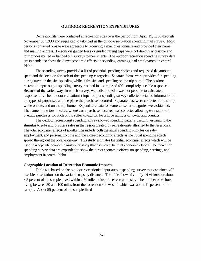
OUTDOOR RECREATION EXPENDITURES

Recreationists were contacted at recreation sites over the period from April 15, 1998 throughNovember 30, 1998 and requested to take part in the outdoor recreation spending mail survey. Mostpersons contacted on-site were agreeable to receiving a mail questionnaire and provided their nameand mailing address. Persons on guided tours or guided rafting trips were not directly accessible andtour guides mailed or handed out surveys to their clients. The outdoor recreation spending survey dataare expanded to show the direct economic effects on spending, earnings, and employment in centralIdaho.

The spending survey provided a list of potential spending choices and requested the amountspent and the location for each of the spending categories. Separate forms were provided for spendingduring travel to the site, spending while at the site, and spending on the trip home. The outdoorrecreation input-output spending survey resulted in a sample of 402 completely useable responses. Because of the varied ways in which surveys were distributed it was not possible to calculate aresponse rate. The outdoor recreationist input-output spending survey collected detailed information onthe types of purchases and the place the purchase occurred. Separate data were collected for the trip,while on-site, and on the trip home. Expenditure data for some 26 seller categories were obtained. The name of the town nearest where each purchase occurred was collected allowing estimation ofaverage purchases for each of the seller categories for a large number of towns and counties.

The outdoor recreationist spending survey showed spending patterns useful in estimating thestimulus to jobs and business sales in the region created by recreationists attracted to the reservoirs. The total economic effects of sportfishing include both the initial spending stimulus on sales,employment, and personal income and the indirect economic effects as the initial spending effectsspread throughout the local economy. This study estimates the initial economic effects which will beused in a separate economic multiplier study that estimates the total economic effects. The recreationspending survey data are expanded to show the direct economic effects on spending, earnings, andemployment in central Idaho.

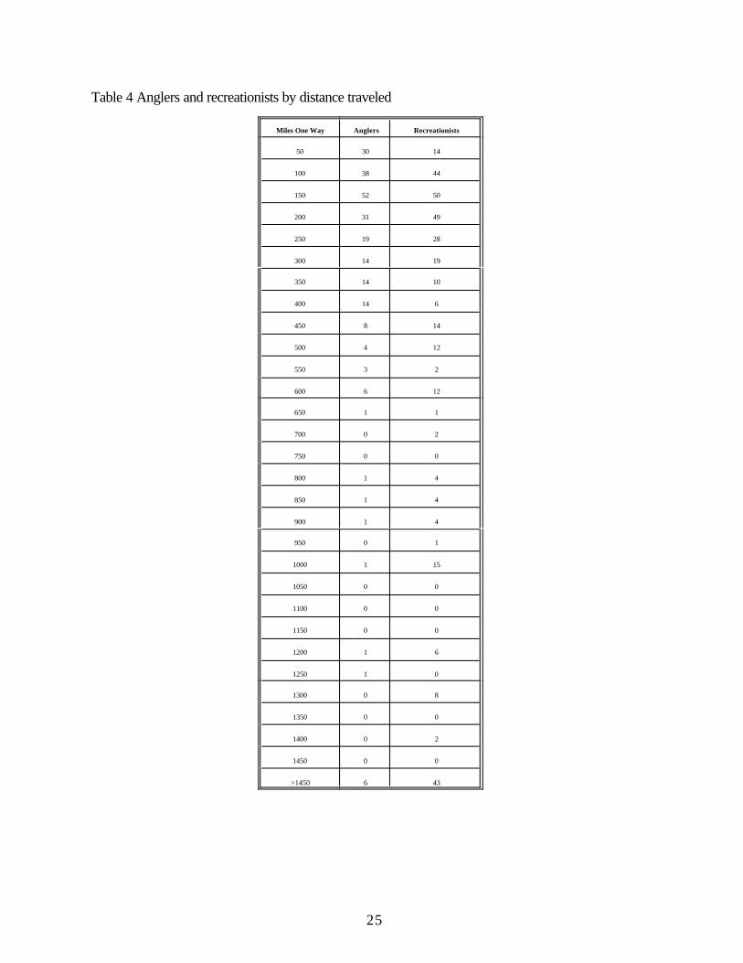
Geographic Location of Recreation Economic ImpactsTable 4 is based on the outdoor recreationist input-output spending survey that contained 402

useable observations on the variable trips by distance. The table shows that only 14 visitors, or about3.5 percent of the sample, lived within a 50 mile radius of the recreation site. The number of visitorsliving between 50 and 100 miles from the recreation site was 44 which was about 11 percent of thesample. About 55 percent of the sample lived

25

Table 4 Anglers and recreationists by distance traveled

Miles One Way Anglers Recreationists

50 30 14

100 38 44

150 52 50

200 31 49

250 19 28

300 14 19

350 14 10

400 14 6

450 8 14

500 4 12

550 3 2

600 6 12

650 1 1

700 0 2

750 0 0

800 1 4

850 1 4

900 1 4

950 0 1

1000 1 15

1050 0 0

1100 0 0

1150 0 0

1200 1 6

1250 1 0

1300 0 8

1350 0 0

1400 0 2

1450 0 0

>1450 6 43

26

Table 5 Spending by recreationists traveling to Central Idaho.

Type of Purchase

AverageExpenditure per

Outdoor RecreationGroup

County Government $1.84

State Government $8.23

Federal Government $0.97

Bus/Taxi $4.16

Tour Boat $50.69

Airline $108.19

Auto/Truck/RV Rental $16.29

Service Station #1 $24.98


Grocery Store $25.27

Auto Dealer $61.34

Clothing Store $9.32

Boat/Marine Store $126.00

Sporting Goods Store $8.19

Hardware Store $1.24

Restaurant $37.64

Department Store $2.30

Other Retail $3.32

Lodging $57.91

Guide Services $144.73

Equipment Rental $9.98

Parking & Car Wash $1.25

Auto Repair $6.53

Other Repair $1.13

Entertainment $9.80

Health Services $0.65

All Other Purchases $18.54

27

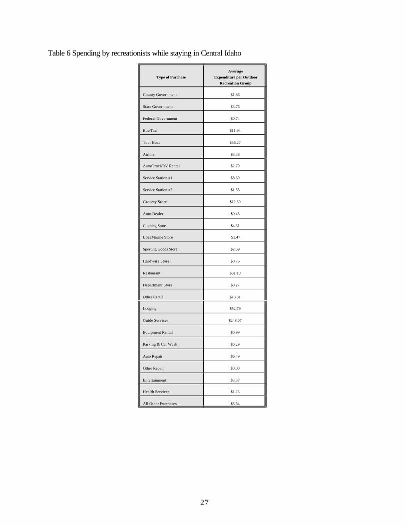
Table 6 Spending by recreationists while staying in Central Idaho

Type of PurchaseAverage

Expenditure per OutdoorRecreation Group




Bus/Taxi $11.94

Tour Boat $56.27

Airline $3.36




Grocery Store $12.39

Auto Dealer $0.45





Restaurant $31.10


Other Retail $13.81

Lodging $52.79




Auto Repair $6.49

Other Repair $0.00

Entertainment $3.37



28

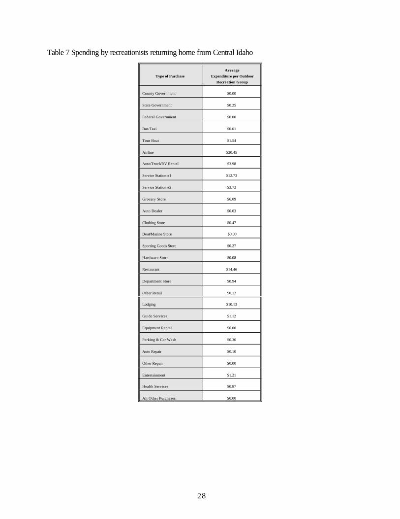
Table 7 Spending by recreationists returning home from Central Idaho

Type of PurchaseAverage

Expenditure per OutdoorRecreation Group




Bus/Taxi $0.01

Tour Boat $1.54

Airline $20.45




Grocery Store $6.09

Auto Dealer $0.03





Restaurant $14.46


Other Retail $0.12

Lodging $10.13




Auto Repair $0.10

Other Repair $0.00

Entertainment $1.21



12 In contrast, the spending survey on the four Lower Snake River reservoirs found that 64 percent of the samplelived within 50 miles of the reservoirs where they recreated.

13 Based on the data from the spending survey for recreationists and estimates of the number of anglers visiting theUpriver Subregion.

14 Our survey question for group size was misinterpreted as rafting group size resulting in an overstated value. Average group size of 1.7305 was from an economic impact study of rafting on the Middle Fork of the Salmon Riverin Idaho (English and Bowker 1996).

29

within 400 miles of the sites in central Idaho where they recreated.12

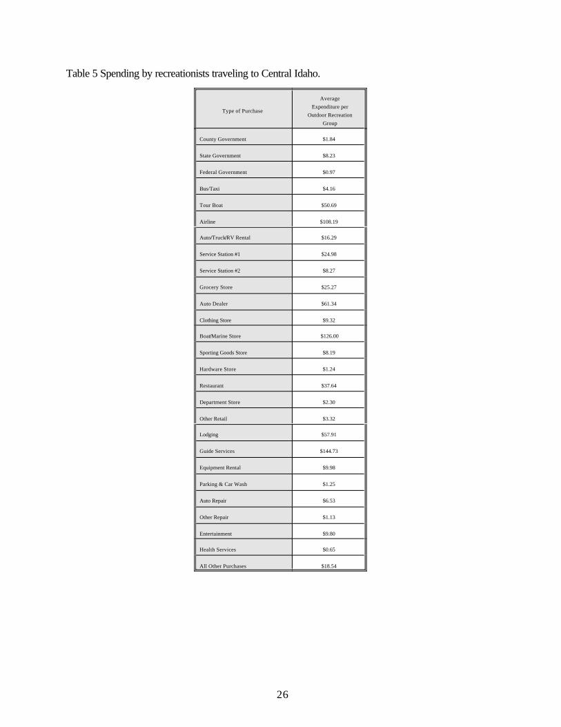
Expenditure Per Visitor per Year and Total Annual SpendingSumming the detailed expenditures collected in the spending survey and shown in Tables 5 - 7

results in a spending total of $1,307.71 x 402 = $525,699 for the 402 recreationist groups in thesurvey.

Total annual spending by all travelers visiting central Idaho was estimated at $298.8 million peryear (1998 dollars). Visitor spending by county was taken from reports prepared for Idaho Division ofTourism Development and for the Oregon tourism Commission, Economic Development Departmentby Dean Runyan Associates. Data for 1996 and 1997 were inflated to 1998 using the consumer priceindex. We estimated that $162.8 million per year was spent by anglers13 in central Idaho leaving $136million per year attributed to non-angler river recreationists. Dividing the annual river recreationspending ($136 million) by our survey average annual spending per recreationist group ($1,307.71)yields 104,000 non-angling recreationist groups. Group size was 1.7305 resulting in 104,000 x 1.7305= 180,000 unique river recreationists.14 Annual spending per river recreationist is $136million/180,000 = $755.55 per year.

Recreation Expenditure Rates by TownThe database collected by the outdoor recreation spending survey allows detailed measurement

of spending by community or county, by type of purchase, and by travel to site, on-site, or return trip. For example, for every 100 recreationists visiting the recreation sites, a specified town or county willhave so many dollars of sales by each economic sector during the trip to the recreation site, while on-site and on the return trip. Towns where outdoor recreationist spending occurred are identified in thedatabase.

15 The travel cost demand survey in central Idaho was conducted concurrent with the spending survey.

30

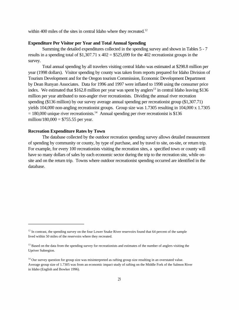
Table 8 Overnight lodging by anglers.

Type of Lodging Percent of Anglers

Camper 4.42%

Trailer 4.73%

Commercial Campground 6.31%

Motel 12.62%

With Friends 3.79%

Public Campground 15.77%

Didn’t Stay Overnight 13.25%

Other Lodging 39.11%

Recreation Lodging

About 87 percent of 317 recreationists in the travel cost demand survey15 stayed overnight atthe recreation site. Table 8 shows that, of those recreationists that do stayovernight, only a small fraction stay at motels or commercial campgrounds. Most of the overnightersstayed in campers, trailers, tents, or in other accommodations.

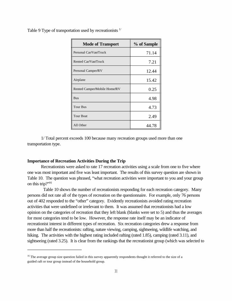
Recreation Mode of TransportationMethod of travel used by the 402 recreationists in the input-output spending survey sample was

classified into eight categories as shown in Table 9. As expected, personal car/van/truck dominated thetransport method. Airplane was second most likely to be used for transport (excluding the All Othercategory).

16 The average group size question failed in this survey apparently respondents thought it referred to the size of aguided raft or tour group instead of the household group.

31

Table 9 Type of transportation used by recreationists 1/

Mode of Transport % of Sample

Personal Car/Van/Truck 71.14

Rented Car/Van/Truck 7.21

Personal Camper/RV 12.44

Airplane 15.42

Rented Camper/Mobile Home/RV 0.25

Bus 4.98

Tour Bus 4.73

Tour Boat 2.49

All Other 44.78

1/ Total percent exceeds 100 because many recreation groups used more than one transportation type.

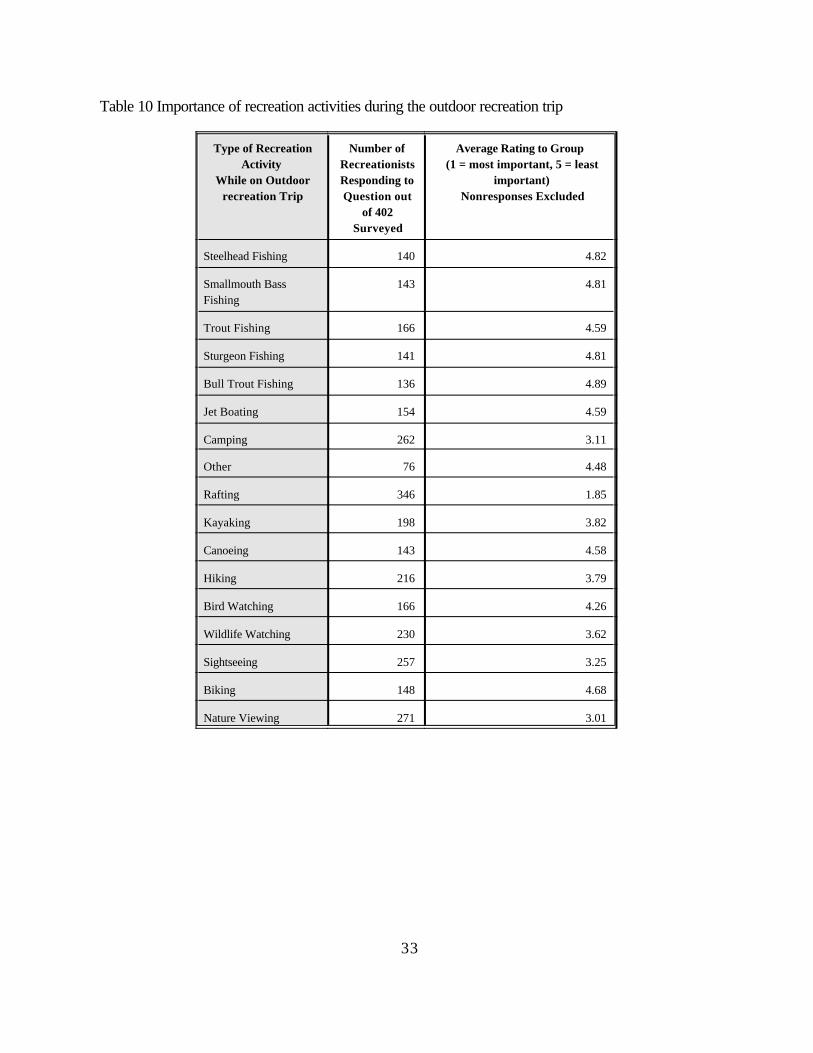
Importance of Recreation Activities During the TripRecreationists were asked to rate 17 recreation activities using a scale from one to five where

one was most important and five was least important. The results of this survey question are shown inTable 10. The question was phrased, “what recreation activities were important to you and your groupon this trip?”16

Table 10 shows the number of recreationists responding for each recreation category. Manypersons did not rate all of the types of recreation on the questionnaire. For example, only 76 personsout of 402 responded to the “other” category. Evidently recreationists avoided rating recreationactivities that were undefined or irrelevant to them. It was assumed that recreationists had a lowopinion on the categories of recreation that they left blank (blanks were set to 5) and thus the averagesfor most categories tend to be low. However, the response rate itself may be an indicator ofrecreationist interest in different types of recreation. Six recreation categories drew a response frommore than half the recreationists: rafting, nature viewing, camping, sightseeing, wildlife watching, andhiking. The activities with the highest rating included rafting (rated 1.85), camping (rated 3.11), andsightseeing (rated 3.25). It is clear from the rankings that the recreationist group (which was selected to

32

exclude primary anglers) visits central Idaho rivers mainly to engage in nature viewing, wildlife watching,camping, and sight seeing while rafting or while hiking.

33

Table 10 Importance of recreation activities during the outdoor recreation trip

Type of RecreationActivity

While on Outdoorrecreation Trip

Number ofRecreationistsResponding toQuestion out

of 402Surveyed

Average Rating to Group (1 = most important, 5 = least

important)Nonresponses Excluded

Steelhead Fishing 140 4.82

Smallmouth BassFishing

143 4.81

Trout Fishing 166 4.59

Sturgeon Fishing 141 4.81

Bull Trout Fishing 136 4.89

Jet Boating 154 4.59

Camping 262 3.11

Other 76 4.48

Rafting 346 1.85

Kayaking 198 3.82

Canoeing 143 4.58

Hiking 216 3.79

Bird Watching 166 4.26

Wildlife Watching 230 3.62

Sightseeing 257 3.25

Biking 148 4.68

Nature Viewing 271 3.01

34

REFERENCES

Adamowicz, W.L., J.J. Fletcher, and T. Graham-Tomasi. 1989. "Functional Form and the StatisticalProperties of Welfare Measures." American Journal of Agricultural Economics 71:414-420.

Becker G.S. "A Theory of the Allocation of Time." 1965. Economic Journal 75:493-517.

Binkley, D., and T.C. Brown. 1993. Management Impacts on Water Quality of Forests andRangelands. USDA Forest Service. GT Report RM-239. Rocky Mountain Forest andRange Experiment Station:Fort Collins.

Bishop, R.C., and T.A. Heberlein. 1979. “Measuring Values of Extra-Market Goods: AreIndirect Measures Biased?” American Journal of Agricultural Economics61(5):926-932.

Bockstael, N.E., and K.E. McConnell. 1981. "Theory and Estimation of the Household ProductionFunction for Wildlife Recreation." Journal of Environmental Economics and Management8:199-214.

Bockstael, N.E., Strand, I.E., and W.M. Hanemann. 1987. "Time and the Recreational DemandModel." American Journal of Agricultural Economics 69:293-302.

Bowker, J.M., English, Donald B.K., and J.A. Donavan. 1996. “Toward a Value for Guided Raftingon Southern Rivers.” Journal of Agricultural and Applied Economics 28,2:423-432.

Brown, W.G., and F. Nawas. 1973. “Impact of Aggregation on the Estimation of SportfishingDemand Functions.” American Journal of Agricultural Economics 55:246-49.

Cameron, A., and P. Trivedi. 1990. “Regression Based Tests for Overdispersion in thePoisson Model.” Journal of Econometrics 46:347-364.

Cameron, T.A., W.D. Shaw, S.E. Ragland, J. Callaway, and S. Keefe. 1996. “Using Actual andContingent Behavior Data with Differing Levels of Time Aggregation to Model RecreationDemand.” Journal of Agricultural and Resource Economics 21(1):130-149.

Caulkins, P.P., R.C. Bishop, and N.W. Bouwes. 1985. "Omitted Cross-Price Variable Biases in theLinear Travel Cost Model: Correcting Common Misperceptions." Land Economics 61:182-87.

35

Clawson, M. and J.L. Knetsch. 1966. Economics of Sportfishing. Johns Hopkins UniversityPress:Baltimore.

Cramer, J.S. 1986. Econometric Applications of Maximum Likelihood Methods. CambridgeUniversity Press:Cambridge. 208pp.

Creel, M.D., and J.B. Loomis. 1990. "Theoretical and Empirical Advantages of Truncated CountData Estimators for Analysis of Deer Hunting in California." American Journal ofAgricultural Economics 72:434-41.

Creel, M.D., and J.B. Loomis. 1991. "Confidence Intervals for Welfare Measures with Application toa Problem of Truncated Counts." The Review of Economics and Statistics 73:370-373.

Crow, E.L., F.A. Davis, and M.W. Maxfield. Undated. Statistics Manual. Research Department,U.S. Naval Ordnance Test Station. Dover Publications, Inc:New York.

Dhrymes, P.J. 1978. Introductory Econometrics. Springer-Verlag:New York. 288pp.

Donnelly, D.M., J.B. Loomis, C.F. Sorg, and L.J. Nelson. 1983. Net Economic Value ofRecreational Steelhead Sportfishing in Idaho. Resource Bulletin RM-9. Rocky MountainForest and Range Experiment Station. USDA Forest Service. Fort Collins, Colorado.

Englin, J., and J.S. Shonkwiler. 1995. "Estimating Social Welfare Using Count Data Models: AnApplication to Long-Run Recreation Demand Under Conditions of Endogenous Stratificationand Truncation." The Review of Economics and Statistics :104-112.

Englin, J., D. Lambert, and W.D. Shaw. 1997. “A Structural Equations Approach to ModelingConsumptive Recreation Demand.” Journal of Environmental Economics andManagement 33:33-43.

English, Donald B.K., and J.M. Bowker. 1996. “Economic Impacts of Guided Whitewater Rafting: AStudy of Five Rivers.” Water Resources Bulletin 32(6):1319-1328.

English, Donald B.K., and J.M. Bowker. 1996. “Sensitivity of Whitewater Rafting Consumers Surplusto Pecuniary Travel Cost Specifications.” Journal of Environmental Management 47:79-91.

Fiore, J., and F.A. Ward. 1987. Managing Recreational Water Resources to Increase EconomicBenefits to Recreationists in the Arid Southwest. Agricultural Experiment Station. ReportNo. 609. New Mexico State University, New Mexico.

36

Fletcher, J.J., W.L. Adamowicz, and T. Graham-Tomasi. 1990. “The Travel Cost Model ofRecreation Demand: Theoretical and Empirical Issues.” Leisure Sciences 12:119-147.

Greene, W.H. 1992. LIMDEP, Version 6. Econometric Software, Inc.:Bellport, New York.

Greene, W.H. 1981. "On the Asymptotic Bias of Ordinary Least Squares Estimator of the TobitModel." Econometrica 49:505-13.

Gum, R., and W.E. Martin. 1975. “Problems and Solutions in Estimating The Demand for the Valueof Rural Sportfishing.” American Journal of Agricultural Economics 57:558-66.

Hellerstein, D.M. 1991. "Using Count Data Models in Travel Cost Analysis with Aggregate Data." American Journal of Agricultural Economics 73:860-67.

Hellerstein, D.M., and R. Mendelsohn. 1993. "A Theoretical Foundation for Count Data Models." American Journal of Agricultural Economics 75:604-611.

Herfindahl, O.C., and A.V. Kneese. 1974. Economic Theory of Natural Resources. Charles E. Merril Publishing Co.:Columbus, Ohio. 405pp.

Johnson, D.M. 1989. Economic Benefits of Alternative Fishery Management Programs. Ph.D.Dissertation. Colorado State University. Fort Collins, Colorado.

Johnson, T.G. 1983. “Measuring the Cost of Time in Recreation Demand: Comment.” AmericanJournal of Agricultural Economics 65:169-171.

Kmenta, J. Elements of Econometrics. 1971. The MacMillan Company:New York. 391-396

Larson, D.M. 1993. "Joint Recreation Choices and Implied Values of Time." Land Economics69(3):270-86.

Layman, R.C., J.R. Boyce, and K.R. Criddle. 1996. “Economic Valuation of the Chinook SalmonSport Fishery of the Gulkana River, Alaska, Under Current and Alternate Management Plans.” Land Economics 72(1):113-28.

Loomis, J.B. 1997. Recreation Economic Decisions: Comparing Benefits and Costs, SecondEdition. With Richard Walsh. Venture Publishing, Inc.:State College, PA.

Loomis, J.B., Sorg, C.F., and D.M. Donnelly. 1986. "Evaluating Regional Demand Models forEstimating Recreation Use and Economic Benefits: A Case Study." Water ResourcesResearch 22:431-38.

37

Loomis, J.B., B. Roach, F.A. Ward, and R. Ready. 1993. “Reservoir Recreation Demand andBenefits Transfers: Preliminary Results.” Western Regional Research Publication. W-133Benefits and Costs Transfer in Natural Resource Planning.

Maddala, G.S. 1983. Limited Dependent and Qualitative Variables in Econometrics. CambridgeUniversity Press:Cambridge.

Maddala, G.S. 1977. Econometrics. International Student Edition. McGraw-Hill BookCompany:Singapore.

Maler, K.G. 1974. Environmental Economics: A Theoretical Inquiry. Johns HopkinsUniversity:Baltimore.

McConnell, K.E. and I.E. Strand. 1981. "Measuring the Cost of Time In Recreational DemandAnalysis: An Application to Sportfishing." American Journal of Agricultural Economics63:153-56.

McConnell, K.E. and I. Strand. 1983. "Measuring the Cost of Time in Recreation Demand Analysis:Reply." American Journal of Agricultural Economics 65:172-74.

McConnell, K.E. 1992. "On-Site Time in Recreation Demand." American Journal of AgriculturalEconomics 74:918-25.

McKean, J.R., and D.M. Johnson. 1998. “Experiments with Equilibrium and Disequilibrium LaborMarket Travel Cost Models.” In Review. 34pp.

McKean, J.R., R.G. Taylor, G. Alward, and R.A. Young. Forthcoming 1998. “Adapting SynthesizedInput-Output Models for Small Natural Resource-Based Regions: A Case Study.” Society andNatural Resources, An International Journal.

McKean, J.R., and R.G. Walsh. 1986. “Neoclassical Foundations for Nonmarket BenefitsEstimation.” Natural Resource Modeling 1:153-170.

McKean, J.R., and C. Revier. 1990. "An Extension of 'Omitted Cross-Price Variable Biases in theLinear Travel Cost Model: Correcting Common Misperceptions." Land Economics 66:162-82.

McKean, J.R., D.M. Johnson, and R.G. Walsh. 1995. "Valuing Time in Travel Cost DemandAnalysis: An Empirical Investigation." Land Economics 71:96-105.

38

McKean, J.R., R.G. Walsh, and D.M. Johnson. 1996. “Closely Related Good Prices in the TravelCost Model.” American Journal of Agricultural Economics 78:640-646.

McKean, J.R., and K.C. Nobe. 1983. Sportsmen Expenditures for Hunting and Sportfishing inColorado - 1981. Technical Report No. 39. Colorado Water Resources Research Institute,Colorado State University and Colorado Division of Wildlife.

McKean, J.R., and K.C. Nobe. 1984. Direct and Indirect Economic Effects of Hunting andSportfishing in Colorado - 1981. Technical Report No. 45. Colorado Water ResourcesResearch Institute, Colorado State University and Colorado Division of Wildlife. Fort Collins,Colorado.

Mendelsohn, R., J. Hof, and G.L. Peterson. 1992. "Measuring Recreation Values with Multiple-Destination Trips." American Journal of Agricultural Economics 74:926-33.

Mullahy, R. 1986. Specification and Testing of Some Modified Count Data Models.” Journal ofEconometrics 33:341-365.

Normandeau Associates, University of Idaho, and Agricultural Enterprises, Inc. 1998a. Sport FisheryUse and Value on Lower Snake River Reservoirs. Phase I Report: Volume 1 of 2. Reservoir Sport Fishery during 1997. Contract No. DACW68-D-0003. US Army Corpsof Engineers, Walla Walla District, Walla Walla, Washington.

Normandeau Associates, Agricultural Enterprises, Inc., and University of Idaho. 1998b. SportFishery Use and Value on Lower Snake River Reservoirs. Phase I Report: Volume 2 of 2. Willingness-To-Pay and Direct Expenditures by Anglers on the Lower Snake RiverReservoirs. Contract No. DACW68-96-D-0003. US Army Corps of Engineers, WallaWalla District, Walla Walla, Washington.

Normandeau Associates, University of Idaho, and Agricultural Enterprises. 1998c. Sport FisheryUse and Value on the Free-Flowing Snake River Above Lewiston, Idaho. Phase IIReport: Volume 1 of 2. Free-Flowing River Sport Fishery During 1997-1998. ContractNo. DACW68-96-D-0003. US Army Corps of Engineers, Walla Walla District, Walla Walla,Washington.

Normandeau Associates, Agricultural Enterprises, Inc., and University of Idaho. 1998d. SportfishingUse and Value on the Free Flowing Snake River Above Lewiston, Idaho. Phase IIReport: Part 2 of 2. Willingness-To-Pay by Anglers on the Free-Flowing Snake RiverDuring 1997-1998. Contract No. DACW68-96-D-0003. US Army Corps of Engineers,Walla Walla District, Walla Walla, Washington.

39

Olsen, D., J. Richards, and R.D. Scott. 1991. “Existence and Sport Values for Doubling the Size of Columbia River Basin Salmon and Steelhead Runs.” Rivers 2(1):44-56.

Oster, J.M., D.T. Taylor, J.J. Jacobs, and E.B. Bradley. 1987. Reservoir Entrophication and theValue of Recreation Activities: A Case Study of Flaming Gorge Reservoir. Department ofAgricultural economics and Wyoming Water Research Center. University of Wyoming. Laramie, Wyoming.

Palm, R.C., and S. P. Malvestuto. 1983. “Relationships Between Economic Benefit and Sport-Sportfishing Effort on West Point Reservoir, Alabama-Georgia.” Transactions of theAmerican Fisheries Society. Page 112.

Parsons, G.R. 1991. “A Note on Choice of Residential Location in Travel Cost Demand Models.” Land Economics 67(3):360-64.

Peterson, G.L., C.S. Swanson, D.W. McCollum, and M.H. Thomas, Eds. 1992. Valuing WildlifeResources in Alaska. Westview Press:Boulder, CO. 357pp.

Randall, A. 1994. “A Difficulty with the Travel Cost Method.” Land Economics 70(1):88-96.

Reading, Don. 1996. The Economic Impact of Steelhead Fishing and the Return of SalmonFishing in Idaho. Ben Johnson Associates. For the Idaho Fish and Wildlife Foundation.

Reading, Don. 1999. The Economic Impact of A Restored Salmon Fishery in Idaho. Ben JohnsonAssociates. For the Idaho Fish and Wildlife Foundation.

Rosenthal, D.H. 1987. "The Necessity for Substitute Prices in Recreation Demand Analyses". American Journal of Agricultural Economics 69:828-37.

Shaw, W.D. 1992. "Searching for the Opportunity Cost of an Individual's Time." Land Economics68:107-15.

Shaw, D. 1988. "On-Site Samples’ Regression Problems of Non-Negative Integers, Truncation andEndogenous Stratification." Journal of Econometrics 37:211-223.

University of Idaho, Department of Fish and Wildlife; Agricultural Enterprises, Inc.; and NormandeauAssociates. 1998. Phase I Report: Volume 2 of 2, Reservoir Sport Fishery During 1997. Sport Fishery Use and Value on Lower Snake River Reservoirs. Department of the Army. Corps of Engineers. Walla Walla District. Walla Walla, Washington.

40

University of Idaho, Department of Fish and Wildlife; Agricultural Enterprises, Inc.; and NormandeauAssociates. 1998. Phase II Report: Volume 2 of 2, Free Flowing River Sport FisheryDuring 1997-1998. Sport Fishery Use and Value on Lower Snake River Reservoirs. Department of the Army. Corps of Engineers. Walla Walla District. Walla Walla,Washington.

U.S. Army Corps of Engineers. 1995. Columbia River System Operation Review, FinalEnvironmental Impact Statement, Appendix O, Economic and Social Impact.

U.S. Army Corps of Engineers. 1995. Columbia River System Operation Review, FinalEnvironmental Impact Statement, Appendix J-1, Recreation Demand Model &Simulation Results.

U.S. Army Corps of Engineers. 1995. Columbia River System Operation Review, FinalEnvironmental Impact Statement, Appendix J, Recreation.

U.S. Water Resources Council. 1983. Economic and Environmental Principles and Guidelinesfor Water and Related Land Resources Implementation Studies. U.S. Government PrintingOffice.

Wade, W.W., G.M. McColister, R.J. McCann, and G.M. Johns. 1988. “Estimating RecreationBenefits for Instream and Diverted Users of Waterflows of the Sacramento-San Joaquin RiversWatershed.” Presented at the W-133 Meeting. Monterey, California.

Walsh, R.G., D.M. Johnson, and J.R. McKean. 1988. Review of Sportfishing Economic DemandStudies with Nonmarket Benefit Estimates 1978-1988. Colorado Water ResourcesResearch Institute. Technical Report No. 54. Colorado State University, Fort Collins,Colorado.

Walsh, R.G., J.R. McKean, and D.M. Johnson. 1988. “Benefit Transfer of Sportfishing DemandStudies, 1968-88.” Water Resources Research 28(3):707-713.

Walsh, R.G., G.L. Peterson, and J.R. McKean. 1989. "Distribution and Efficiency Effects ofAlternative Recreation Funding Methods." Journal of Leisure Research 21:327-47.

Walsh, R.G., J.R. McKean, and D.M. Johnson. 1990a. “Nonmarket Values from Two Decades ofResearch on Recreation Demand.” In Advances in Applied Microeconomics, Vol. V. V.K.Smith and A.N. Link Eds. JAI Press, Inc.:Greenwich, Conn. Pp. 167-194.

Walsh, R.G., L.D. Sanders, and J.R. McKean. 1990b. "The Consumptive Value of Travel Time onRecreation Trips." Journal of Travel Research 29:17-24.

41

Ward, F.A. 1983. "Measuring the Cost of Time in Recreation Demand Analysis: Comment." American Journal of Agricultural Economics 65:167-68.

Ward, F.A. 1989. “Efficiently Managing Spatially Competing Water Uses: New Evidence from aRegional Recreation Demand Model.” Journal of Regional Science 29(2):229-46.

Ward, F.A. 1984. "Specification Considerations for the Price Variable in Travel Cost DemandModels." Land Economics 60:301-5.

Whitehead, J.C. 1991-92. “Benefits of Quality Changes in Recreational Sportfishing: A Single-SiteTravel Cost Approach.” Journal of Environmental Systems 21(4):357-64.

Wilman, E.A. 1980. "The Value of Time in Recreation Benefit Studies." Journal of EnvironmentalEconomics and Management 7:272-86.

Wilman, E.A., and R.J. Pauls. 1987. “Sensitivity of Consumers’ Surplus Estimates toVariation in the Parameters of the Travel Cost Model.” Canadian Journal ofAgricultural Economics 35:197-211.

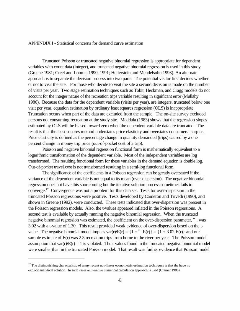
17 The distinguishing characteristic of many recent non-linear econometric estimation techniques is that the have noexplicit analytical solution. In such cases an iterative numerical calculation approach is used (Cramer 1986).

42

APPENDIX I - Statistical concerns for demand curve estimation

Truncated Poisson or truncated negative binomial regression is appropriate for dependentvariables with count data (integer), and truncated negative binomial regression is used in this study(Greene 1981; Creel and Loomis 1990, 1991; Hellerstein and Mendelsohn 1993). An alternateapproach is to separate the decision process into two parts. The potential visitor first decides whetheror not to visit the site. For those who decide to visit the site a second decision is made on the numberof visits per year. Two stage estimation techniques such as Tobit, Heckman, and Cragg models do notaccount for the integer nature of the recreation trips variable resulting in significant error (Mullahy1986). Because the data for the dependent variable (visits per year), are integers, truncated below onevisit per year, equation estimation by ordinary least squares regression (OLS) is inappropriate. Truncation occurs when part of the data are excluded from the sample. The on-site survey excludedpersons not consuming recreation at the study site. Maddala (1983) shows that the regression slopesestimated by OLS will be biased toward zero when the dependent variable data are truncated. Theresult is that the least squares method understates price elasticity and overstates consumers’ surplus.Price elasticity is defined as the percentage change in quantity demanded (trips) caused by a onepercent change in money trip price (out-of-pocket cost of a trip).

Poisson and negative binomial regression functional form is mathematically equivalent to alogarithmic transformation of the dependent variable. Most of the independent variables are logtransformed. The resulting functional form for these variables in the demand equation is double log. Out-of-pocket travel cost is not transformed resulting in a semi-log functional form.

The significance of the coefficients in a Poisson regression can be greatly overstated if thevariance of the dependent variable is not equal to its mean (over-dispersion). The negative binomialregression does not have this shortcoming but the iterative solution process sometimes fails toconverge.17 Convergence was not a problem for this data set. Tests for over-dispersion in thetruncated Poisson regressions were positive. Tests developed by Cameron and Trivedi (1990), andshown in Greene (1992), were conducted. These tests indicated that over-dispersion was present inthe Poisson regression models. Also, the t-values appeared inflated in the Poisson regressions. Asecond test is available by actually running the negative binomial regression. When the truncatednegative binomial regression was estimated, the coefficient on the over-dispersion parameter, ", was3.02 with a t-value of 1.30. This result provided weak evidence of over-dispersion based on the t-value. The negative binomial model implies var(r)/E(r) = {1 + " E(r)} = {1 + 3.02 E(r)} and oursample estimate of E(r) was 2.3 recreation trips from home to the river per year. The Poisson modelassumption that var(r)/E(r) = 1 is violated. The t-values found in the truncated negative binomial modelwere smaller than in the truncated Poisson model. That result was further evidence that Poisson model

43

had over-dispersion. Therefore, the truncated negative binomial regression technique was used in placeof truncated Poisson regression.

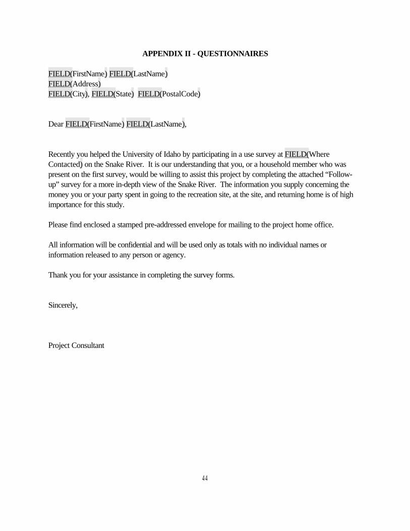
44

APPENDIX II - QUESTIONNAIRES

FIELD(FirstName) FIELD(LastName)FIELD(Address)FIELD(City), FIELD(State) FIELD(PostalCode)

Dear FIELD(FirstName) FIELD(LastName),

Recently you helped the University of Idaho by participating in a use survey at FIELD(WhereContacted) on the Snake River. It is our understanding that you, or a household member who waspresent on the first survey, would be willing to assist this project by completing the attached “Follow-up” survey for a more in-depth view of the Snake River. The information you supply concerning themoney you or your party spent in going to the recreation site, at the site, and returning home is of highimportance for this study.

Please find enclosed a stamped pre-addressed envelope for mailing to the project home office.

All information will be confidential and will be used only as totals with no individual names orinformation released to any person or agency.

Thank you for your assistance in completing the survey forms.

Sincerely,

Project Consultant

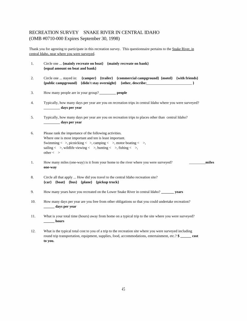
45

RECREATION SURVEY SNAKE RIVER IN CENTRAL IDAHO(OMB #0710-000 Expires September 30, 1998)

Thank you for agreeing to participate in this recreation survey. This questionnaire pertains to the Snake River, incentral Idaho, near where you were surveyed.

1. Circle one ... {mainly recreate on boat} {mainly recreate on bank} {equal amount on boat and bank}

2. Circle one ... stayed in: {camper} {trailer} {commercial campground} {motel} {with friends} {public campground} {didn't stay overnight} {other, describe:_________________________ }

3. How many people are in your group? _________ people

4. Typically, how many days per year are you on recreation trips in central Idaho where you were surveyed?_________ days per year

5. Typically, how many days per year are you on recreation trips to places other than central Idaho?_________ days per year

6. Please rank the importance of the following activities. Where one is most important and ten is least important.Swimming < >, picnicking < >, camping < >, motor boating < >, sailing < >, wildlife viewing < >, hunting < >, fishing < >, other < >

1. How many miles (one-way) is it from your home to the river where you were surveyed? _________milesone-way

8. Circle all that apply ... How did you travel to the central Idaho recreation site?{car} {boat} {bus} {plane} {pickup truck}

9. How many years have you recreated on the Lower Snake River in central Idaho? _______ years

10. How many days per year are you free from other obligations so that you could undertake recreation? ______ days per year

11. What is your total time (hours) away from home on a typical trip to the site where you were surveyed? ______ hours

12. What is the typical total cost to you of a trip to the recreation site where you were surveyed including round trip transportation, equipment, supplies, food, accommodations, entertainment, etc.? $ ______ cost to you.

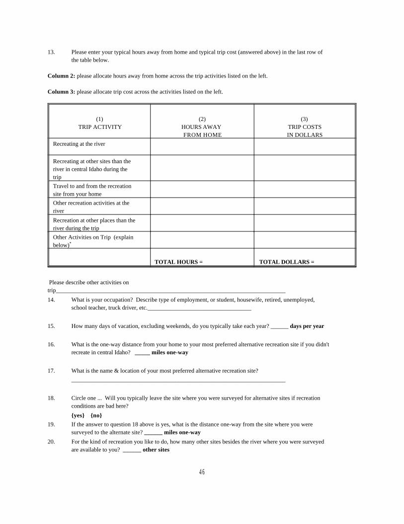
46

13. Please enter your typical hours away from home and typical trip cost (answered above) in the last row ofthe table below.

Column 2: please allocate hours away from home across the trip activities listed on the left.

Column 3: please allocate trip cost across the activities listed on the left.

(1)TRIP ACTIVITY

(2)HOURS AWAY FROM HOME

(3)TRIP COSTSIN DOLLARS

Recreating at the river

Recreating at other sites than theriver in central Idaho during thetripTravel to and from the recreationsite from your homeOther recreation activities at theriver

Recreation at other places than theriver during the tripOther Activities on Trip (explainbelow)*

TOTAL HOURS = TOTAL DOLLARS =

Please describe other activities ontrip_____________________________________________________________________________

14. What is your occupation? Describe type of employment, or student, housewife, retired, unemployed,school teacher, truck driver, etc.___________________________________

15. How many days of vacation, excluding weekends, do you typically take each year? ______ days per year

16. What is the one-way distance from your home to your most preferred alternative recreation site if you didn'trecreate in central Idaho? _____ miles one-way

17. What is the name & location of your most preferred alternative recreation site?________________________________________________________________________

18. Circle one ... Will you typically leave the site where you were surveyed for alternative sites if recreationconditions are bad here?

{yes} {no}19. If the answer to question 18 above is yes, what is the distance one-way from the site where you were

surveyed to the alternate site? ______ miles one-way

20. For the kind of recreation you like to do, how many other sites besides the river where you were surveyedare available to you? ______ other sites

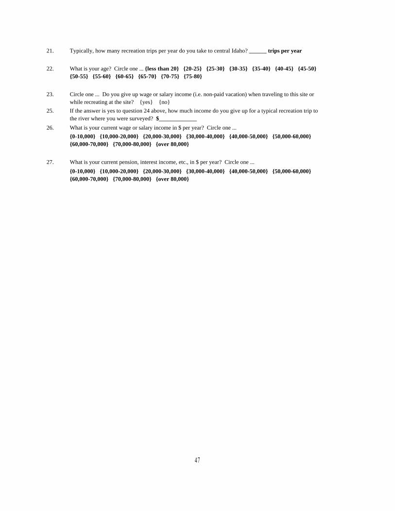
47

21. Typically, how many recreation trips per year do you take to central Idaho? ______ trips per year

22. What is your age? Circle one ... {less than 20} {20-25} {25-30} {30-35} {35-40} {40-45} {45-50} {50-55} {55-60} {60-65} {65-70} {70-75} {75-80}

23. Circle one ... Do you give up wage or salary income (i.e. non-paid vacation) when traveling to this site orwhile recreating at the site? {yes} {no}

25. If the answer is yes to question 24 above, how much income do you give up for a typical recreation trip tothe river where you were surveyed? $_____________

26. What is your current wage or salary income in $ per year? Circle one ... {0-10,000} {10,000-20,000} {20,000-30,000} {30,000-40,000} {40,000-50,000} {50,000-60,000} {60,000-70,000} {70,000-80,000} {over 80,000}

27. What is your current pension, interest income, etc., in $ per year? Circle one ...

{0-10,000} {10,000-20,000} {20,000-30,000} {30,000-40,000} {40,000-50,000} {50,000-60,000} {60,000-70,000} {70,000-80,000} {over 80,000}

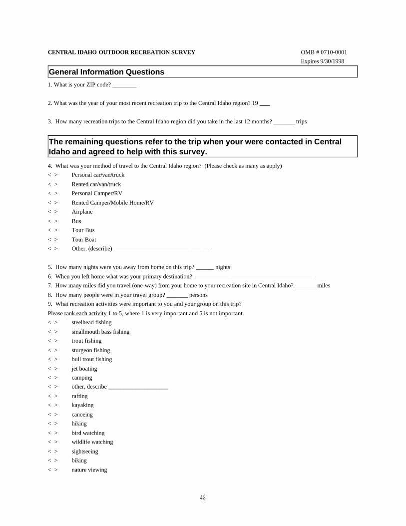
48

CENTRAL IDAHO OUTDOOR RECREATION SURVEY OMB # 0710-0001 Expires 9/30/1998

General Information Questions1. What is your ZIP code? ________

2. What was the year of your most recent recreation trip to the Central Idaho region? 19

3. How many recreation trips to the Central Idaho region did you take in the last 12 months? _______ trips

The remaining questions refer to the trip when your were contacted in CentralIdaho and agreed to help with this survey.

4. What was your method of travel to the Central Idaho region? (Please check as many as apply)< > Personal car/van/truck

< > Rented car/van/truck< > Personal Camper/RV

< > Rented Camper/Mobile Home/RV< > Airplane

< > Bus< > Tour Bus

< > Tour Boat< > Other, (describe) ________________________________

5. How many nights were you away from home on this trip? ______ nights

6. When you left home what was your primary destination? _______________________________________7. How many miles did you travel (one-way) from your home to your recreation site in Central Idaho? _______ miles

8. How many people were in your travel group? _______ persons9. What recreation activities were important to you and your group on this trip?

Please rank each activity 1 to 5, where 1 is very important and 5 is not important.< > steelhead fishing

< > smallmouth bass fishing< > trout fishing

< > sturgeon fishing< > bull trout fishing

< > jet boating< > camping< > other, describe ____________________

< > rafting< > kayaking

< > canoeing< > hiking

< > bird watching< > wildlife watching

< > sightseeing< > biking

< > nature viewing

49

<

A map is enclosed that shows the Central Idaho region. Please use the map toidentify local stopping points on your trip when answering the questions on thefollowing pages.

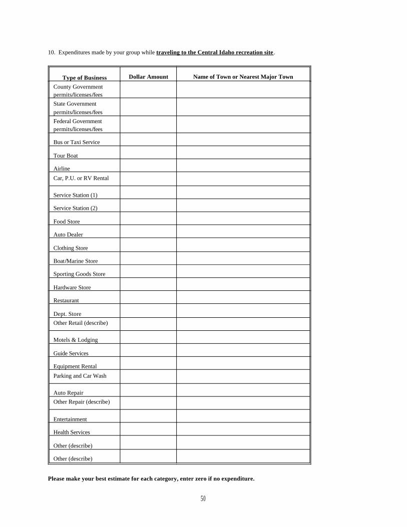
50

10. Expenditures made by your group while traveling to the Central Idaho recreation site .

Type of Business Dollar Amount Name of Town or Nearest Major Town

County Governmentpermits/licenses/feesState Governmentpermits/licenses/feesFederal Governmentpermits/licenses/fees

Bus or Taxi Service

Tour Boat

Airline

Car, P.U. or RV Rental

Service Station (1)

Service Station (2)

Food Store

Auto Dealer

Clothing Store

Boat/Marine Store

Sporting Goods Store

Hardware Store

Restaurant

Dept. StoreOther Retail (describe)

Motels & Lodging

Guide Services

Equipment Rental

Parking and Car Wash

Auto RepairOther Repair (describe)

Entertainment

Health Services

Other (describe)

Other (describe)

Please make your best estimate for each category, enter zero if no expenditure.

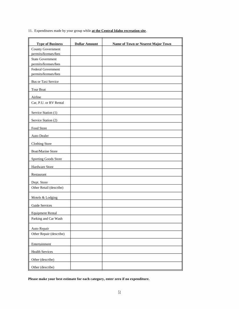
51

11. Expenditures made by your group while at the Central Idaho recreation site .

Type of Business Dollar Amount Name of Town or Nearest Major TownCounty Governmentpermits/licenses/feesState Governmentpermits/licenses/feesFederal Governmentpermits/licenses/fees

Bus or Taxi Service

Tour Boat

Airline


Service Station (1)

Service Station (2)

Food Store

Auto Dealer

Clothing Store

Boat/Marine Store


Hardware Store

Restaurant


Motels & Lodging

Guide Services

Equipment Rental



Entertainment

Health Services

Other (describe)

Other (describe)


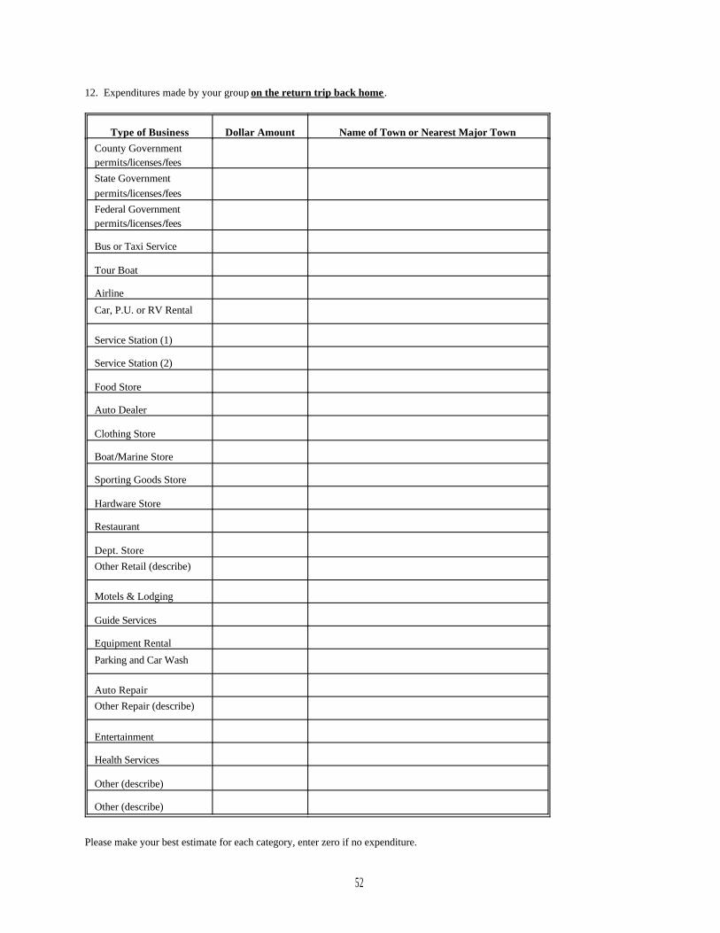
52

12. Expenditures made by your group on the return trip back home .

Type of Business Dollar Amount Name of Town or Nearest Major TownCounty Governmentpermits/licenses/feesState Governmentpermits/licenses/feesFederal Governmentpermits/licenses/fees

Bus or Taxi Service

Tour Boat

Airline


Service Station (1)

Service Station (2)

Food Store

Auto Dealer

Clothing Store

Boat/Marine Store


Hardware Store

Restaurant


Motels & Lodging

Guide Services

Equipment Rental



Entertainment

Health Services

Other (describe)

Other (describe)


Documents

OUTDOOR RECREATION USE AND VALUE: