Outer Billiards and The Pinwheel Map

Richard Evan Schwartz ∗

May 12, 2011

1 Introduction

1.1 Background

B. H. Neumann [N] introduced outer billiards in the late 1950s and J. Moser[M1] popularized the system in the 1970s as a toy model for celestial mechan-ics. Outer billiards is a discrete self-map of R2 − P , where P is a boundedconvex planar set as in Figure 1.1 below. Given x1 ∈ R

2 −P , one defines x2so that the segment x1x2 is tangent to P at its midpoint and P lies to theright of the ray −−→x1x2. The map x1 → x2 is called the outer billiards map.The map is almost everywhere defined and invertible.

2

P1

Figure 1.1: Outer billiards relative to P .

∗ Supported by N.S.F. Research Grant DMS-0072607

1

There has been a fair amount of work on outer billiards in the past 30years. See, for instance, [D], [DF], [G], [GS], [Ko], [M2], [S1], [S2], [T2],[VS]. The book [T1] has a nice survey, though this survey misses some ofthe recent work.

Let ψ denote the second iterate of the outer billiards map on a convexpolygon P . The purpose of this paper is to establish an equivalence betweenψ and an auxilliary map ψ∗ which we call the pinwheel map. For convenience,we work with convex polygons that have no parallel sides, and henceforthwe make this assumption. The general case introduces tedious complicationswhich we prefer to avoid. The pinwheel map is defined in terms of a certainfamily of strips associated to P . We first define these strips and explain theirconnection to ψ.

V

w

v L

Σ

L’

P

eFigure 1.2: The strip associated to e.

We orient the edges of P so someone walking along an edge in the directionof the orientation would see P on the right. Given an edge e of P , we letL be the line extending e and we let L′ be the line parallel to L so that thevertex w of P that lies farthest from L is equidistant from L and L′. Weassociate to e the pair (Σ, V ), where Σ is the strip bounded by L and L′, andV = 2(w − v). See Figure 1.2. We call (Σ, V ) a pinwheel pair and we call Σa pinwheel strip.

We label the edges e1, ..., en in such a way that the lines l1, ..., ln occur incounterclockwise cyclic order. Here lk is the line through the origin parallelto ek. We correspondingly label the pinwheel pairs (Σ1, V1), ...(Σn, Vn). Notethat these labellings do not typically correspond to the cyclic ordering of theedges around the boundary of P . See Figure 1.4 below for an example.

2

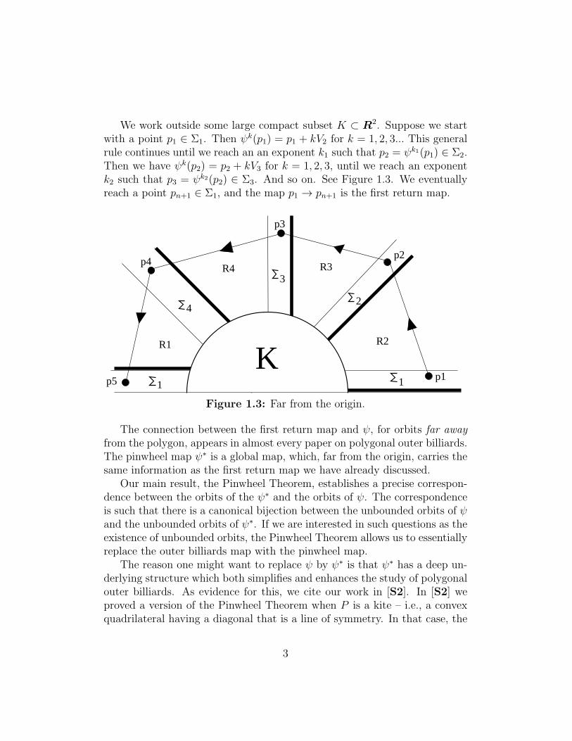
We work outside some large compact subset K ⊂ R2. Suppose we start

with a point p1 ∈ Σ1. Then ψk(p1) = p1 + kV2 for k = 1, 2, 3... This general

rule continues until we reach an an exponent k1 such that p2 = ψk1(p1) ∈ Σ2.Then we have ψk(p2) = p2 + kV3 for k = 1, 2, 3, until we reach an exponentk2 such that p3 = ψk2(p2) ∈ Σ3. And so on. See Figure 1.3. We eventuallyreach a point pn+1 ∈ Σ1, and the map p1 → pn+1 is the first return map.

1

2

R2

R3R4

p1

p2

p3

p4

p5

R1

1

4

3

KFigure 1.3: Far from the origin.

The connection between the first return map and ψ, for orbits far awayfrom the polygon, appears in almost every paper on polygonal outer billiards.The pinwheel map ψ∗ is a global map, which, far from the origin, carries thesame information as the first return map we have already discussed.

Our main result, the Pinwheel Theorem, establishes a precise correspon-dence between the orbits of the ψ∗ and the orbits of ψ. The correspondenceis such that there is a canonical bijection between the unbounded orbits of ψand the unbounded orbits of ψ∗. If we are interested in such questions as theexistence of unbounded orbits, the Pinwheel Theorem allows us to essentiallyreplace the outer billiards map with the pinwheel map.

The reason one might want to replace ψ by ψ∗ is that ψ∗ has a deep un-derlying structure which both simplifies and enhances the study of polygonalouter billiards. As evidence for this, we cite our work in [S2]. In [S2] weproved a version of the Pinwheel Theorem when P is a kite – i.e., a convexquadrilateral having a diagonal that is a line of symmetry. In that case, the

3

pinwheel map has a kind of compactification as a higher dimensional poly-tope exchange map. See [S2, Master Picture Theorem]. Some version of thishigher dimensional compactification of the Pinwheel Map works in general,though we have not yet worked it out. The Pinwheel Theorem, which allowsone to relate outer billiards to this higher dimensional compact dynamicalsystem, seems to be a good first step towards a general theory of polygonalouter billiards.

1.2 The Main Result

Now we will define the pinwheel map precisely. The n pinwheel stripsΣ1, ...,Σn are ordered as above (according to their slopes). Given the pair(Σ, V ), we define a map µ on R

2 − ∂Σ as follows.

• If x ∈ Σ− ∂Σ then µ(x) = x.

• If x 6∈ Σ then µ(x) = x± V , whichever point is closer to Σ.

The map µ moves points “one step” closer to lying in Σ, if they don’t alreadylie in Σ. Note that µ is not defined on the boundary ∂Σ.

Let R2

n = R2 × 1, ..., n, with indices taken mod n. We define the

pinwheel map ψ∗ : R2

n → R2

n by the following conditions.

• ψ∗(p, j) = (µj+1(p), j + 1) if µj+1(p) = p.

• ψ∗(p, j) = (µj+1(p), j) if µj+1(p) 6= p.

In other words, we try to move p by the (j + 1)st strip map. If the pointdoesn’t move, we increment the index and give the next strip map a chanceto move the point.

Let π : R2

n → R2 be the projection map. We introduce a map

ι : R2 → R2

n, (1)

which we call the pinwheel section. This map has the property that π ι isthe identity.

4

13

5

42

1

2

34

5

Figure 1.4: The Pinwheel Section in the case n = 5.

As shown in Figure 1.4 for the case n = 5, in general we extend the edgesof the polygon and then label the regions 1, ..., n. The region k correspondsto the edge ek. As above, these edges are ordered according to their slopes.Our result takes its name from the pinwheel-like appearance of Figure 1.4.

If p lies in the interior of the region labelled a, we define ι(p) = (p, a− 1).If p is not in the interior of any of the labelled regions, we define the secondcoordinate of ι(p) any way we like. For such points, the relevant maps areundefined.

Theorem 1.1 (Pinwheel) Relative to the pinwheel section ι, we have

ψ(p) = π (ψ∗)k ι; k = k(p) ∈ 1, ..., 3n.

This relation holds on all points for which ψ is well defined.

Far from the origin, we have k(p) = 1 unless p lies in a pinwheel strip. Inthis case k(p) = 2 because one extra iterate of ψ∗ is required to shift the index.Figure 1.5 shows the example of a regular pentagon, with p lying just aboveone of the vertices. In this case k(p) = 3 and the pinwheel map successivelyadds the vector 2A, 2B, and 2C. At the same time, ψ(p) = p + 2D. Inthis case, we have the “cancellation” A+ B + C = D. Similar cancellationsalways occur when k(p) > 2.

5

D

p

A

B C

Figure 1.5: A+ B + C = D.

The bound k(p) ≤ 3n is not sharp, but one can easily generalize theexample in Figure 1.5 to show that k(p) = n−2 is attained, in some examples,for all n. We think that the bound k(p) ≤ n− 2 is sharp.

1.3 Corollaries

Just from knowledge of the relation between ψ and ψ∗ far from the origin,one can conclude nothing about how the unbounded orbits of one systemcompare to the unbounded orbits of the other.

Figure 1.6: Systems which agree outside a compact set.

Figure 1.6 suggests an example of two dynamical systems which agreeoutside a compact set, in which one has unbounded orbits and the otherdoes not. The top shows an infinite union of rectangles. The n-th rectangleintersects R at −1 + 1/n and n. The bottom shows a spiral obtained by

6

modifying the union of rectangles within a compact set. Both systems aredefined as (say) the time one maps of the unit speed flows along the curves.We leave it to the interested reader to flesh out this example.

In light of the work in [S2], which exhibits unbounded outer billiardsorbits that return infinitely often to a compact region of the plane, one mightworry that the pinwheel map and the outer billiards map are somehow relatedas are the maps suggested in Figure 1.6. The Pinwheel Theorem rules outthis possibility.

We say that an unbounded orbit of ψ∗ is natural if it lies in ι(R2) suffi-ciently far from the origin.

Corollary 1.2 Relative to any convex polygon having no parallel sides, thereis a canonical bijection between the forward (respectively, backward or two-sided) unbounded ψ-orbits and the natural forward (respectively backward ortwo-sided) unbounded ψ∗-orbits. The bijection sending the orbit O to theorbit O∗ is such that O = π(O∗) outside a compact subset.

One reason why one might want to study ψ∗ in place of ψ is that ψ∗ hasan appealing acceleration. Define

X =n⋃

j=1

(Σj × j) ⊂ R2

n. (2)

Topologically, X is the disjoint union of n strips. X agrees with ι(⋃Σj)

outside a compact set. We let ψ : X → X be the first return map of ψ∗ toX.

Corollary 1.3 There is a canonical bijection between the forward (respec-tively backward or two-sided) unbounded orbits of ψ and the forward (respec-

tively backward or two-sided) unbounded orbits of ψ.

The map Ψ = (ψ)n preserves each individual strip in X. The action oneach strip is conjugate to the action on any of the other ones, outside of acompact set. Thus, we can pick one of the strips, say Σ1, and consider themap Ψ : Σ1 → Σ1. We call Ψ the pinwheel return map.

At the same time, we can consider the first return map of ψ to Σ1, as wedid informally above. We call this map Ψ.

Corollary 1.4 There is a canonical bijection between the forward (respec-tively backward or two-sided) unbounded orbits Ψ and the forward (respec-

tively backward or two-sided) unbounded orbits of Ψ.

7

1.4 Outline of the Paper

In §2 we prove a number of combinatorial and geometric results about con-structions related to convex polygons. In §3 we prove all the results, modulotwo lemmas, Lemma 3.7 and Lemma 3.8. In §4 we prove Lemma 3.8 and§5 we prove Lemma 3.7. Ultimately, the argument boils down to robustgeneral properties like convexity and induction, but only after we find thecombinatorial structure of what is going on.

1.5 Pinwheel Applet

My java applet, Pinwheel , to be found athttp://www.math.brown.edu/∼res/Pinwheel/Main.htmlillustrates the Pinwheel theorem in great detail. The applet has its ownsummary of the result, though doesn’t go so far as to give a proof. Thereader might want to first play with the applet to get a general sense of whatis going on visually.

1.6 Acknowledgements

I would like to thank John Smillie and Sergei Tabachnikov for helpful con-versations about outer billiards and the pinwheel map. In particular, theformulation we give of the Pinwheel Theorem emerged in conversations withSmillie. Finally, I’d like to thank the anonymous referee for many helpfulexpository suggestions.

I would also like to thank the Clay Mathematics Institute for their supportduring my sabbatical two years ago, when I worked out the material in thispaper.

8

2 Preliminaries

2.1 Basic Definitions

Throughout the chapter, P is a convex polygon with no parallel sides. Letψ′ be the outer billiards map and let ψ = (ψ′)2.

The Forward Partition: We have already mentioned that ψ is a piece-wise translation. For almost every point p ∈ R

2 − P , there is a pair ofvertices (vp, wp) of P such that vp is the midpoint of the segment connectingp and ψ′(p) and wp is the midpoint of the segment connecting ψ′(p) and ψ(p).In this case, we have

ψ(p) = p+ Vp; Vp = 2(wp − vp). (3)

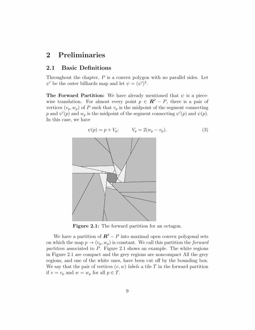
Figure 2.1: The forward partition for an octagon.

We have a partition of R2 − P into maximal open convex polygonal setson which the map p→ (vp, wp) is constant. We call this partition the forwardpartition associated to P . Figure 2.1 shows an example. The white regionsin Figure 2.1 are compact and the grey regions are noncompact All the greyregions, and one of the white ones, have been cut off by the bounding box.We say that the pair of vertices (v, w) labels a tile T in the forward partitionif v = vp and w = wp for all p ∈ T .

9

Spokes: We have already associated n vectors to our n-gon P , namely thepinwheel vectors V1, ..., Vn defined in connection with Figure 1.2. We let Sk

be the line segment that joins the head and tail of Vk. We call Sk a spoke.The spoke Sk is essentially an undirected version of Vk. Figure 2.2 shows anexample, with some of the edges highlighted.

e7

e3

e5

e6

e1

45

1

3

27

6

v

w

e2

e4

Figure 2.2: The spokes of the polygon, and the path 7 → 3.

Admissible Paths: Recall that the spokes are cyclically ordered accordingto their slopes. We say that an oriented, connected polygonal path γ isadmissible if the following holds.

• γ consists of an odd number of spokes of P .

• The ordering on the spokes of γ is compatible with the cyclic order.

• Let γ′ be the polygonal path in R ∪ ∞ obtained by connecting theslopes of the spokes of γ. Then γ′ is a proper subset of R ∪∞.

The last condition means that γ does not wrap all the way around P . Weuse the notation a → b to name admissible paths. The first spoke is a andthe last one is b. We often take the indices mod n and use b+n in place of bin case b < a. Thus, 7 → 10 is another name for the the path in Figure 2.2.

10

Maximal Pairs: We say that a pair of vertices (v, w) of P is maximalif and only they are the endpoints of a spoke. Here is an equivalent charac-terization: (v, w) is maximal if and only if there is an infinite strip T suchthat P ⊂ T and ∂T ∩P = v, w. This equivalence uses the fact that P hasno parallel sides.

Admissible Pairs: A pair (v, w) of vertices of P is admissible if thereis a maximal pair (v, x) such that v, w, x occur in clockwise order on ∂P . Weallow the possibility that w = x, so that maximal pairs count as admissible.We mention, without giving the easy proof, that if (v, w) and (w, v) are bothadmissible than (v, w) is maximal.

The Clockwise Correspondence: As we illustrated in Figure 1.2, weassociate the pinwheel pair (Σj, Vj) to the edge ej of P . We let Sj be thespoke corresponding to Vj. We call the correspondence ej → Sj the clockwisecorrespondence. This correspondence is a bijection. (See Lemma 2.2 for aproof.) The segments Sj, Sj+1, and ej form the sides of a triangle.

Pinwheel Orientation: Recall that Sj is just an undirected version of Vj.When we want to assign an orientation to Sj, we say that oriented(Sj) = Vj.We call this the pinwheel orientation on Sj.

Special and Ordinary Spokes: We say that a spoke S2 of P is specialif there are spokes S1 and S3 such that S1, S2, S3 share a common vertex. Wecall the remaining spokes ordinary . In Figure 2.2, the spokes S1 and S3 arespecial and the rest are ordinary.

The Edge Set: Let e1, ..., en be the edges of P and let S1, ..., Sn be thecorresponding spokes. We take indices mod n, so that the objects ea+kn

and Sa+kn refer to the same objects ea and Sa for all k ∈ Z. Suppose thata < b < a+ n are two integers. We define the edge set

V (a, b) = E ∪X; X =b−1⋃

i=a

ei; X = Sa ∩ Sb ∩ ∂P. (4)

X is empty unless Sa and Sb share a common vertex. Figure 2.3 shows V (a, b)in two cases. V (a, b) is highlighted in grey.

11

a Sb SbSaS

Figure 2.3: The set V (a, b).

2.2 The Structure of Spokes

Here we prove a few combinatorial results about spokes. Figure 2.2 gives anice illustration of these results.

Lemma 2.1 Every two spokes intersect.

Proof: Suppose that S and S ′ are disjoint spokes. Let T and T ′ be infinitestrips corresponding to S and S ′ respectively. Both points of S ′ lie on thesame side of ∂P − ∂T . This fact, and the convexity of P , forces ∂T and ∂T ′

to be parallel. But then T = T ′, and ∂P ∩ ∂T consists of two edges. This isa contradiction. ♠

Lemma 2.2 When the spokes are ordered according to their slopes, Sj andSj+1 are consecutive. In particular, the clockwise correspondence betweenedges and spokes is a bijection.

Proof: We identify the set of slopes of lines with RP1, the projective line.

The edges Sj, Sj+1, and ej form a triangle τ and Sj+1 is obtained from Sj

by rotating Sj counterclockwise about the vertex uj of τ opposite ej. LetIj ⊂ RP

1 be the set of slopes of lines joining points of ej to uj . Any otherspoke Sk intersects both Sj and Sj+1, and from this property we see thatthe intervals Ij and Ik have disjoint interiors when j 6= k. Furthermore, theunion

⋃j Ij is exactly RP

1. Our lemma follows from this structure. ♠

12

Lemma 2.3 The edges ej and ej+1 are adjacent if and only if Sj+1 is aspecial spoke.

Proof: Without loss of generality, we set j = 1. If S2 is a special spoke,then the spokes S1, S2, S3 all share a common point. The other three pointsare the vertices of the arc e1 ∪ e2. Hence e1 and e2 are adjacent. Conversely,suppose e1 and e2 are adjacent. Then the each of the 3 vertices of e1 ∪ e2 isa vertex of some Sj for j = 1, 2, 3. This forces the vertex S1 ∩ S2 to equalthe vertex S2 ∩ S3. Hence S2 is special. ♠

Lemma 2.4 Let γ be an admissible path of length at least 3. The orienta-tion on the spokes of γ induced by the orientation on γ coincides with thepinwheel orientation on all edges but the last one. On the last spoke, the twoorientations agree if and only if the spoke is ordinary.

Proof: We make two observations: First, for the first edge of an admissiblepath, the pinwheel orientation coincides with the path orientation. See Fig-ure 2.2. Second, suppose that S1, ..., Sk are consecutive spokes all sharing acommon vertex v. When these spokes are given the pinwheel ordering, thecommon vertex v is the head vertex of S2, ..., Sk and the tail vertex of S1.This lemma follows from the two observations and induction. ♠

2.3 The Structure of the Edge Set

For this whole section, we choose two integers a and b with a < b < a + n.Here n is the number of sides of P .

Lemma 2.5 V (a, b) has two connected components, both having their end-points in Sa ∪ Sb.

Proof: The proof goes by induction on b − a. When b − a = 1, we haveV (a, b) = ea ∪ (Sa ∩ Sa+1), the union of an edge and a vertex. In this case,the result is clear from the basic fact that Va, Va+1 and ea make a triangle.When b − a > 1, we have V (a, b) = V (a, b − 1) ∪ eb−1. We simply adjointhe edge eb−1 to one component of V (a, b) or the other, and use the fact thatSb−a, Sb, and eb−1 make a triangle. ♠

13

Lemma 2.6 Let e be an edge of V (a, b). Let v be the vertex of P that isfarthest from the line extending e. Then v is a point of the component ofV (a, b) that does not contain e.

Proof: Let S be the spoke corresponding to e. Then S intersects both Sa

and Sb. One endpoint of S is a vertex of e. So, by Lemma 2.5, the otherendpoint, namely v, must lie in the other component of V (a, b). ♠

e

S

Sa Sb

v

Figure 2.4: The set V (a, b) and the spoke S.

Lemma 2.7 Let p1, p2, p3 be three consecutive points of an outer billiardsorbit. Let w1 be the midpoint of p1p2 and let w2 be the midpoint of p2p3.Suppose w1 is an endpoint of Sa and w2 is an endpoint of Sb. Then V (a, b)does not separate w1 from w2.

Proof: We will treat the case when Sa and Sb intersect at an interior vertex,so that both components of V (a, b) are finite unions of edges. See Figure 2.5below. The other case has a similar treatment.

Examining our proof of Lemma 2.5, we note that we can describe V (a, b)as follows. As we rotate Sa counterclockwise, through a suitable family ofchords of P , until it reaches Sb, the set V (a, b) is the curve swept out bythe endpoints of the rotating chord. We make this rotating family preciseas follows. Since Sa, Sa+1, ea make a triangle, we can interpolate from Sa toSa+1 by considering the chords that join Sa∩Sa+1 to some point of ea. Thenwe do the same thing for Sa+1 and Sa+2. And so on.

At the same time, (w1, w2) is an admissible pair, so the clockwise arc Ajoining w1 to w2 avoids the interior of V (a, b). Indeed, A is the arc swept outby one of the endpoints of Sa as we rotate it clockwise until it reaches Sb. ♠

14

Sb

w2

a

p1

p2

p3

w1

S

Figure 2.5: The set V (a, b) and part of an outer billiards orbit.

2.4 Admissible Paths and Tiles

Here is the main result in this section.

Lemma 2.8 There is a bijection between tiles in the forward partition andadmissible paths. The tile corresponding to a → b is labelled by the vertexpair (v, w), where v is the first vertex of a→ b and w is the last one.

We will prove this result through a series of three smaller results.

Lemma 2.9 A pair of vertices (v, w) is admissible if and only if v and wrespectively are the starting and ending points of an admissible path.

Proof: Each maximal pair of vertices is clearly admissible. These correspondto single spokes. Conversely, each admissible path of length 1 is an orientedspoke and hence corresponds to a maximal pair of vertices. If we start withan admissible path a → b and minimally lengthen it to the new admissiblepath a→ b′, the new endpoint is a vertex adjacent to, and counterclockwisefrom, the old endpoint. At the same time, the admissible vertices are ob-tained from the maximal vertices by moving the endpoints counterclockwise.Our claim follows from these facts and from induction. ♠

15

Lemma 2.10 There is a bijection between unbounded tiles in the forwardpartition and the maximal pairs of vertices.

Proof: Suppose that p1, p2, p3 are three consecutive points in an outer bil-liards orbit. Let w1 be the midpoint of p1p2 and let w2 be the midpoint ofp2p3. We claim that there is some compact set K such that (w1, w2) is notmaximal only if p1, p2, p3 ∈ K. If this was false, then we could take a limitof counter examples and produce an infinite strip T such that P ⊂ T and∂T ∩ ∂S = w1, w2. Hence, once p1 is sufficiently far from the origin, thetile containing p is labelled by a maximal pair of vertices.

Conversely, let e be an edge of P and let (Σ, V ) be the associated pin-wheel pair. Let v and w be the tail and head vertices of V . We scale so thatthe lines y = 0 and y = 1 bound Σ. If R is sufficiently large, then the tilescontaining (R,−1) and (−R, 2) are respectively labelled by (v, w) and (w, v).These points each lie just outside the strip Σ. ♠

Lemma 2.11 There is a bijection between bounded tiles in the forward par-tition and admissible pairs which are not maximal.

Proof: We use the notation from Lemma 2.10. We write pj(0) = pj and we

let p1(t) be the point that is t units away from p1(0) along the ray−−−−−−→p2(0)p1(0).

Let w1(t) and w2(t) be the vertices that depend on the points pj(t).

As t increases, and p1(t) moves away from the origin, the line p1(t)p2(t)does nothing and the line p2(t)p3(t) rotates clockwise. The vertex w1(t) isindependent of t but the vertex w2(t) moves clockwise away from w1(t) indiscrete jumps. A jump occurs every time p2(t) lies on one of the rays shownin Figure 1.4. When t is sufficiently large (w1(t), w2(t)) is maximal. Hence(w1(0), w2(0)) is admissible.

Since p1(0) lies in a bounded tile and p1(t) lies in an unbounded tile for tsufficiently large, the vertex w2(t) must have made at least 1 jump along theway. Hence the initial pair (w1(0), w2(0)) is not maximal. This shows thateach bounded tile corresponds to an admissible but not maximal pair.

For the converse, our construction shows that each admissible pair arisesas the pair associated to some tile in the forward partition. We first choosep1 so that w1 and w2 are adjacent vertices. We then pull p1 away from P , asdescribed above, and observe that we encounter every admissible pair whoseinitial vertex is w1. ♠

16

2.5 A Result about Strips

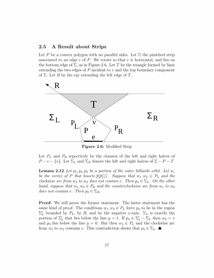
Let P be a convex polygon with no parallel sides. Let Σ the pinwheel stripassociated to an edge e of P . We rotate so that e is horizontal, and lies onthe bottom edge of Σ, as in Figure 2.6. Let T be the triangle formed by linesextending the two edges of P incident to v and the top boundary componentof Σ. Let R be the ray extending the left edge of T .

P

ePR

LL

Σ

R

RΣ vP

T

Figure 2.6: Modified Strip

Let PL and PR repectively be the closures of the left and right halves ofP − e− v. Let ΣL and ΣR denote the left and right halves of Σ− P − T .

Lemma 2.12 Let p1, p2, p3 be a portion of the outer billiards orbit. Let wj

be the vertex of P that bisects pjpj+1. Suppose that w1, w2 ∈ PL and theclockwise arc from w2 to w3 does not contain e. Then p2 ∈ ΣL. On the otherhand, suppose that w1, w2 ∈ PR and the counterclockwise arc from w1 to w0

does not contain e. Then p2 ∈ ΣR.

Proof: We will prove the former statement. The latter statement has thesame kind of proof. The conditions w1, w2 ∈ PL force p2 to lie in the regionΣ′

L bounded by PL, by R, and by the negative x-axis. ΣL is exactly theportion of Σ′

L that lies below the line y = 1. If p2 ∈ Σ′

L − ΣL then w2 = vand p3 lies below the line y = 0. But then w3 ∈ PL and the clockwise arcfrom w2 to w3 contains e. This contradiction shows that p2 ∈ ΣL. ♠

17

2.6 Structure of the Forward Partition

The rays in Figure 1.4 are the sets where the outer billiards map is notdefined. We call these the primary rays . The primary rays separate R

2 − Pinto n distinct cones. Figure 2.7 shows two of these rays and one of the cones.We label the cones C1, ..., Cn, so that Ca contains all the tiles of the formT (a → b). The apex of Ca is a vertex of the spoke Sa, as the labelling inFigure 1.4 indicates.

Figure 2.7 illustrates what the forward partition looks like within a singlecone. The thin segments A,B,C, ... separating the tiles within the cone aremapped, by the outer billiards map, to the primary rays extending the edgeswe have also labelled A,B,C.... All the tile except one are quadrilaterals,and the tile containing the apex of the cone is a triangle.

B

C

B

A

A

C

Figure 2.7: The forward partition within a cone.

The bounded tiles in the cone C = Ca all have a common boundary withthe pinwheel strip Σ = Σa, but are disjoint from Σ. Our next result gives anestimate on the geometry of these tiles.

18

Lemma 2.13 Let τ be any bounded tile in C. No point of τ is farther from∂Σ than half the width of Σ.

Proof: We rotate so that Σ is horizontal, as in Figure 2.8. The line throughv1 is the centerline of Σ. Let T be the union of all the bounded tiles in C.Let w be the edge of T opposite the apex v0 of C. Let p0 be the bottomvertex of T . Let p1 be the image of p0 under the outer billiards map. Notethat w is parallel to a line L which extends one of the sides of P . The basicfact is that p1 below the centerline of Σ. But p0 and p1 are equidistant fromthe lower boundary of Σ. Hence the distsance from p0 to the lower boundaryof Σ is less than half the width of Σ. Since p0 is the extreme point of T , thesame statement holds for all points in T . ♠

L

v1p1

v0

p0

w

Σ

C

T

P

Figure 2.8: Bounding the tiles.

Recall that (Σj , Vj) is the pinwheel pair associated to the edge ej of P .Let ∂1Σj be the component of ∂Σj that contains ej. Let ∂2Σj be the othercomponent of ∂Σj. Let T (1 → b) be the tile in the forward partition associ-ated to the admissible path 1 → b.

Lemma 2.14 Suppose 1 < b < n+ 1. If e0 is adjacent to e1 then T (1 → b)and P lie on the same side of ∂1Σ0. Otherwise, T (1 → b) and P lie on thesame side of ∂2Σ0.

19

Proof: Since 1 < b < n + 1, the tile T (1 → b) is bounded. If e0 and e1 areadjacent, then e0 = f0 in Figure 2.9. The shaded cone in Figure 2.9 containsT (1 → b). In this case, the whole shaded cone lies on one side of ∂1Σ0, andthe result is obvious. In the second case, e0 = g0, and we want to rule outthe possibility that T (1 → b) intersects the black cone. But one checks easilythat points in the black cone correspond to the pair (x, y). In this case, theseare the endpoints of the spoke S0. But such points lie in the tiles of the formT (0 → a). This is a contradiction. ♠

yg0

x e1f0

S1

Figure 2.9: The excluded region.

20

3 Proof modulo Two Details

3.1 The Main Argument

Let ι be the pinwheel section. According to Lemma 2.8, there is a bijectivecorrespondence between tiles in the forward partition and admissible paths.We let T (a → b) denote the tile in the forward partition corresponding tothe path a → b. Referring to the discussion in §2.6, we recall that the tileT (a→ b) lies in the cone Ca. But then, by definition of the pinwheel section,

p ∈ T (a→ b); =⇒ ι(p) = (p, a− 1). (5)

Let ψ∗ denote the pinwheel map, defined in §1.2. Below we will prove thefollowing result.

Theorem 3.1 Suppose p ∈ T (a → b) and q = ψ(p) ∈ T (c → d). Then(ψ∗)k(q, b− 1) = (q, c− 1) for some k ∈ 0, ..., n.

We note in Theorem 3.1 that the conclusion of the result only involves thepoint q, but the choice of b in the conclusion comes from the hypothesis thatq = ψ(p) and p ∈ T (a→ b).

We will also prove the following result.

Theorem 3.2 Let a → b be an admissible path, labelled so that a ≤ b. Ifp ∈ T (a→ b) then (ψ∗)k(p, a− 1) = (ψ(p), b− 1) for some k ∈ 1, ..., 2n.

Combining Theorems 3.1 and 3.2, we have the following result.

Corollary 3.3 Let T (a → b) and T (c → d) be two tiles. Suppose that wehave p ∈ T (a → b) and ψ(p) ∈ T (c → d). Then there is some integerk ∈ 0, ..., 3n such that (ψ∗)k(p, a− 1) = (ψ(p), c− 1).

Proof of the Pinwheel Theorem: The map ψ is defined precisely on theinteriors of the tiles in the forward partition. For p in the interior of the tileT (a → b), we have ι(p) = (p, a − 1). As usual, we take the indices mod n.The conclusion of Corollary 3.3 is just a restatement of the equation in thePinwheel Theorem. ♠

Now we prove the corollaries. We will consider the forward orbits. Theother cases are similar.

21

Proof of Corollary 1.2: Let p ∈ R2 be a point with an unbounded forward

ψ-orbit O. We define p∗ = ι(p). Let O∗ be the ψ∗ orbit of p∗. By the PinwheelTheorem, there is an infinite sequence t1, t2, ... such that ιψk(p) = (ψ∗)tk(p∗).This clearly shows that O is forward unbounded if and only if O∗ is forwardunbounded. As we mentioned after stating the Pinwheel Theorem, we havek(p) = 1 when p is sufficiently far from the origin and not contained in apinwheel strip. We have k(p) = 2 when p is sufficiently far from the originand contained in a pinwheel strip. From these properties, it is easy to seethat the following is true for all sufficiently large compact sets K.

π(O∗ −K∗) = O −K; K∗ = π−1(K). (6)

It follows from Equation 6 that there exists only one orbit O∗ such thatπ(O∗ −K) = O −K. Hence, the assignment O → O∗, which first seems todepend on the choice of p, is well defined independent of the choice. If O1

and O2 are different unbounded orbits, they differ outside of K. Hence O∗

1

and O∗

2 differ as well. This shows that the assignment O → O∗ is injective.Recall that an unbounded orbit of ψ∗ is natural if it lies in ι(R2) suffi-

ciently far from the origin. Let O∗ be some unbounded natural orbit. Wejust choose some p ∈ O∗ −K∗ and let p = π(p∗). Then the argument aboveshows that O∗ is the image of O under our correspondence. Hence, our cor-respondence is a bijection. ♠

Proof of Corollary 1.3: In light of Corollary 1.2, we just have to constructa bijection between the set of forward unbounded natural orbits of ψ∗ andthe set of forward unbounded orbits of ψ. But ι(R2) and X agree outsidea compact set. So, suppose that O∗ is a forward unbounded natural orbit.The set O = O∗ ∩ X is a forward unbounded orbit of X. The nature thisconstruction makes it clear that the correspondence O∗ → O is a bijection. ♠

Proof of Corollary 1.4: For each orbit O of ψ, the intersection O ∩ Σ1 isthe corresponding orbit of Ψ. The assignment O → (O∩Σ1) gives a bijectionbetween the set of unbounded orbits of ψ and the set of unbounded orbitsof Ψ. Similarly, there is a canonical bijection between the set of unboundedorbits of ψ and the set of unbounded orbits of Ψ. Finally, Corollary 1.3 givesus a canonical bijection between the unbounded orbits of ψ and the set ofunbounded orbits of ψ. Composing all these bijections gives us the desiredresult. ♠

22

3.2 Proof of Theorem 3.1

We can define the backwards partition for P just as we defined the forwardspartition. We just use the inverse map ψ−1.

The map ψ sets up a bijection between the tiles in the forward partitionand the tiles in the backward partition. A tile in the forward partitionlabelled by a pair of vertices (v, w) corresponds to a tile in the backwardpartition labelled by a pair of vertices (w, v).

We change our notation so that T+(a → b) = T (a → b), and T−(a → b)denotes a tile in the backwards partition corresponding to the “backwardsadmissible path”. The backwards admissible paths have the same definitionas the forwards admissible paths, except that the spokes are traced out inreverse cyclic order. Tautologically, we have

ψ(T+(a→ b)) = T−(b→ a). (7)

If b = c in Theorem 3.1, then we can take k = 0 and there is nothing toprove. So, assume b 6= c. If necessary, we add n to c so that b < c < b+ n.

Lemma 3.4 Let p1, p2, p3 be a portion of the outer billiards orbit. Let wj bethe vertex of P that bisects pjpj+1. Suppose also that p2 ∈ T−(a, b)∩ T+(c, d)for some indices a, d. Then w1 is an endpoint of the spoke Sb and w2 is anendpoint of the spoke Sc.

Proof: By definition the admissible path c→ d has w2 as its first endpointand w3 as its second endpoint. Hence w2 is an endpoint of Sc. The sameargument, applied to the inverse of the outer billiards map, shows that w1 isan endpoint of Sb. ♠

Lemma 3.5 We have T−(a, b) ∩ T+(c, d) ⊂ Σj for all j = b, ..., c− 1.

Proof: By definition, e = ej ⊂ V (b, c), the set defined in §2.1. We rotate sothat e is as in Lemma 2.12. Lemma 2.1 justifies our picture of Sb and Sc ascrossing. Lemma 2.5 justifies our picture of V (b, c) as the union of two arcswhose endpoints lie in Sb ∪ Sc. We have drawn V (b, c) thickly in Figure 4.2.Let v be the vertex of P farthest from the line extending e. Lemma 2.6 saysthat v is a subset of the component of V (b, c) that does not contain e.

23

v

w3

w2

bS

w1e

x

p1

p3

p2

cS

Figure 3.1:

By Lemma 3.4, the point w1 is an endpoint of Sb and the point w2 is anendpoint of Sc. We let PL and PR and ΣL and ΣR be as in Lemma 2.12.We mean for these sets to be defined relative to e and v. Note that onecomponent of ∂P − V (b, c) lies in PL and the other component lies in PR.Hence, by Lemma 2.7, either w1, w2 ∈ PL (as shown) or w1, w2 ∈ PR. Wewill consider the former case. The latter case is similar.

By Lemma 2.8, the pair (w2, w3) is admissible. Hence w2, w3, x occur inclockwise order. Here w2 and x are the two endpoints of Sc. In particular,the arc of ∂P that goes clockwise from w2 to w3 does not contain e. Lemma2.12 now says that p ∈ ΣL ⊂ Σj. ♠

Proof of Theorem 3.1: Our point q in Theorem 3.1 lies in T−(a, b)∩T+(c, d)for some choice of indices a and d. Hence

q ∈ Σj ; j = b, ..., (c− 1).

Henceψ∗(q, j) = (q, j + 1); j = (b− 1), ..., (c− 2).

Hence (ψ∗)k(q, b− 1) = (q, c− 1) for k = b− a < n. ♠

24

3.3 Theorem 3.2 modulo Two Details

We first prove Theorem 3.2 in the case that a = b. In this case a → a isan admissible path of length 1, and the corresponding tile T (a → a) in theforward partition is unbounded. Let p ∈ T (a→ a). By construction

ψ(p) = p+ 2Va (8)

We scale so that ea lies in the x-axis and Σa lies above the x-axis. Theregion T (a → a) contains the point (R,−1) once R is sufficiently large. Inparticular T (a→ a) lies beneath Σa. But then ψ

∗(p, a−1) = (p+2Va, a−1)for all p ∈ T (a→ a). Hence ψ∗(p, a− 1) = (ψ(p), a− 1), as desired.

Now we assume that a < b < a + n. For convenience, we label so thata = 1. The admissible path 1 → b does not necessarily involve all the spokesbetween 1 and b. Let Vi be the ith pinwheel vector and let Si be the ithspoke. If Si is not involved in the path 1 → b, let Wi = 0. Otherwise, let Wi

be the vector that points from the first endpoint of Si to the last one. Herewe are orienting Si according to the admissible path 1 → b.

If Wk is nonzero, and 1 ≤ k < b then, according to Lemma 2.4, we haveWk = Vk. We also have Wb = ±Vb, with the sign depending on whether ornot Sb is a special spoke.

Lemma 3.6 For any p ∈ T (1 → b) we have

ψ(p)− p =b∑

i=1

2Wi.

Proof: Let (v, w) be the admissible pair of vertices associated to T (1 → b).Recall that 1 and b respectively name the first and last spoke of the admissiblepath associated to T (1 → b) whereas v and w respectively name the firstendpoint of the path and the last endpoint of the path. The path 1 → bsimply traces out the involved spokes. By definition

w − v =b∑

i=1

Wi.

At the same time ψ(p)− p = 2(w− v). Putting these two equations togethergives the lemma. ♠

25

Lemma 3.6 establishes an identity between certain multiples of the vectorsinvolved in the relevant strip maps. This is a good start. What connects theresult in Lemma 3.6 to the pinwheel map is the claim that the multiplesinvolved are precisely the ones that arise in the relevant strip maps. Thisamounts to showing that certain translates of the tile T (a → b) lie in theright place with respect to the relevant strips. Define

T (1 → b; k) = T (1 → b) +k∑

i=1

2Wi; k = 1, ..., b (9)

Recall that µb is the strip map associated to the pinwheel pair (Σb, Vb).

Lemma 3.7 T (1 → b; k) ⊂ Σk for all k = a, ..., (b− 1).

Proof: See §4 ♠

Lemma 3.8 µb(p) = p+ 2Wb for all p ∈ T (1 → b, b− 1).

Proof: See §5 ♠

Proof of Theorem 3.2: Let p = p0 ∈ T (1 → k) be an arbitrary point.Define

pk = p0 +k∑

i=1

2Wi; k = 1, ..., b. (10)

We have pk ∈ T (1 → b; k).By Lemma 3.6, we have

ψ(p0) = pb. (11)

Choose any k = 0, 1, ..., b − 2 and consider the pair (pk, k). There aretwo cases to consider. Suppose first that the index k is involved in the path1 → b. Then

pk+1 = pk + 2Wk ∈ T (1 → b; k + 1) ⊂ Σk+1. (12)

The second containment is Lemma 3.8. Therefore

µk+1(pk) = pk + 2Vk = pk + 2Wk = pk+1; µk+1(pk+1) = pk+1. (13)

26

Hence

(ψ∗)2(pk, k) = ψ∗ µk+1(pk, k) = ψ∗(pk+1, k) = (pk+1, k + 1). (14)

Now suppose that the index k is not involved in the path 1 → b. Thenpk+1 = pk and,

pk = pk+1 ∈ T (1 → b; k + 1) ⊂ Σk+1. (15)

Again, the second containment is Lemma 3.8. Hence, by definition,

ψ∗(pk, k) = (pk, k + 1) = (pk+1, k + 1). (16)

In either case, we see that

(pk+1, k + 1) = (ψ∗)e(pk, k); e ∈ 1, 2. (17)

Applying this argument for as long as we can, we see that

(pb−1, b− 1) = (ψ∗)e(p0, 0); e ∈ 1, ..., 2n− 2. (18)

Finally, by Lemma 3.7.

ψ∗(pb−1, b− 1) = (µ∗

b(pb−1), b− 1) = (pb−1 +Wb, b− 1) = (pb, b− 1). (19)

Hence (pb, b − 1) is in the forward ψ∗-orbit of (p0, 0). Combining this infor-mation with Equation 11, we see that there is some positive k < 2n suchthat

(ψ(p), b− 1) = (pb, b− 1) = (ψ∗)k(p, 0). (20)

This completes the proof. ♠

27

4 Proof of Lemma 3.7

4.1 A Technical Lemma

Let W1, ...,Wb be the vectors associated to the admissible path 1 → b, asin the statement of Lemma 3.7. We have W1 = V1. As a special case ofEquation 9, we consider

T (1 → b, 1) = T (1 → b) + 2W1 = T (1 → b) + 2V1. (21)

Lemma 4.1 If S1 is a special spoke, then the line ∂2Σ0 separates P fromT (1 → b; 1). If S1 is an ordinary spoke, then the line ∂1Σ0 separates P fromT (1 → b; 1).

Proof: If S1 is a special spoke, then e0 and e1 are adjacent by Lemma 2.3.Since e0 and e1 are adjacent, the vector V1 joins a a point on ∂1Σ0 to a pointon the centerline of Σ0. Hence ∂1Σ0 + 2V1 = ∂2Σ0. The first case of thislemma now follows from Lemma 2.14. The point is that adding V1 ejectsT (1 → b) outside of Σ0, and onto the correct side.

If S1 is an ordinary spoke then e0 and e1 are not adjacent, Lemma 2.3.This time V1 joins a point on the centerline of Σ0 to a point on ∂2Σ0. Hence∂2Σ0 + 2V1 = ∂1Σ0. The rest of the proof is the same in this case. ♠

4.2 The Conjugate Polygon

Let R : R2 → R2 denote reflection in the x-axis. For any subset A ⊂ R

2, letA = R(A). A basic and easy fact is that R maps the backward partition of Pto the forward partition of P . For that reason, we will consider the forwardpartitions of P and P at the same time. We rotate so that the edge e0 of Pis horizontal and lies in the x-axis, below the rest of P . To emphasize thedependence on P , we write e0(P ), etc. We let e0(P ) be the horizontal edgeof P . Note that e0(P ) lies above the rest of P .

The cyclic ordering forces two sets of equations.

ek(P ) = e−k(P ); Σk(P ) = Σ−k(P ). (22)

Sk(P ) = S1−k(P ); Vk(P ) = V1−k(P ). (23)

28

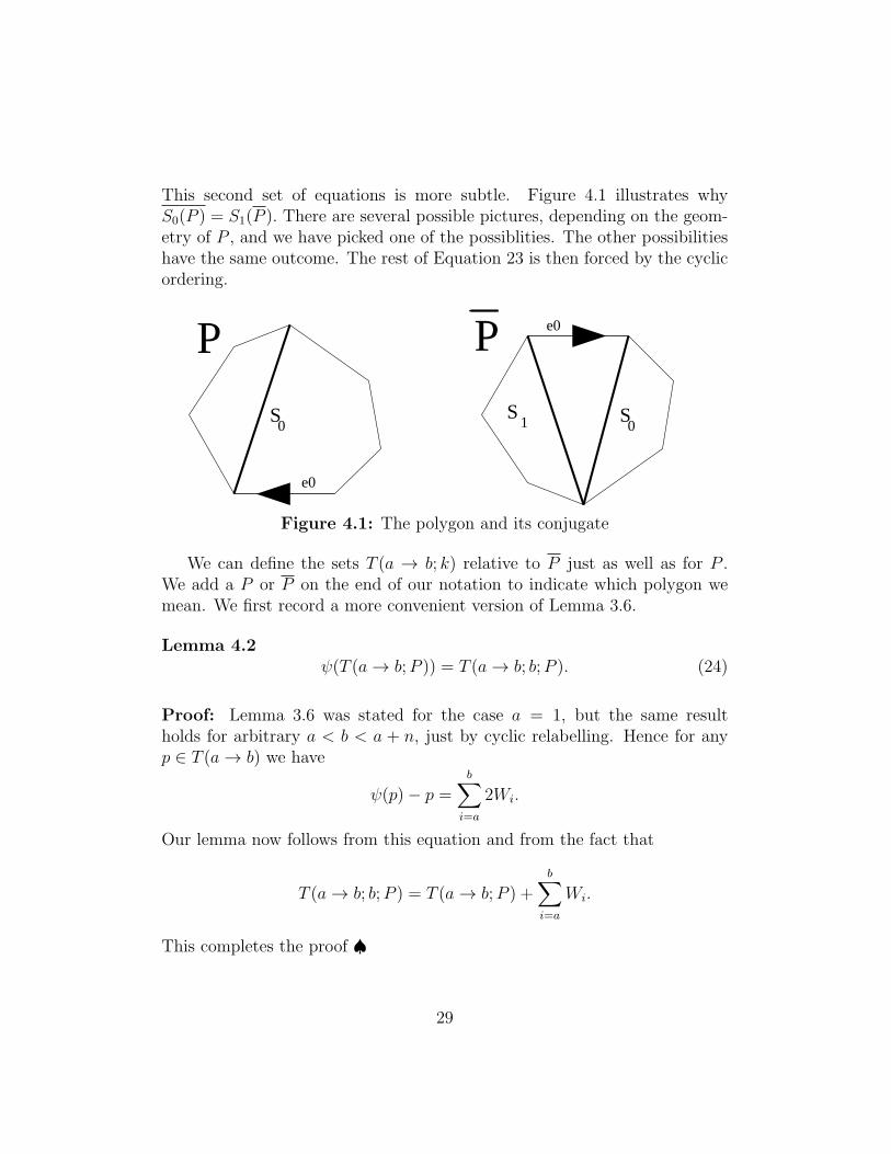
This second set of equations is more subtle. Figure 4.1 illustrates whyS0(P ) = S1(P ). There are several possible pictures, depending on the geom-etry of P , and we have picked one of the possiblities. The other possibilitieshave the same outcome. The rest of Equation 23 is then forced by the cyclicordering.

10S

0

e0

e0P P

SS

Figure 4.1: The polygon and its conjugate

We can define the sets T (a → b; k) relative to P just as well as for P .We add a P or P on the end of our notation to indicate which polygon wemean. We first record a more convenient version of Lemma 3.6.

Lemma 4.2ψ(T (a→ b;P )) = T (a→ b; b;P ). (24)

Proof: Lemma 3.6 was stated for the case a = 1, but the same resultholds for arbitrary a < b < a + n, just by cyclic relabelling. Hence for anyp ∈ T (a→ b) we have

ψ(p)− p =b∑

i=a

2Wi.

Our lemma now follows from this equation and from the fact that

T (a→ b; b;P ) = T (a→ b;P ) +b∑

i=a

Wi.

This completes the proof ♠

29

Before we prove the next result, we note that T (a → b, a − 1;P ) is justT (a → b;P ). We also note that the sets T (1 − b → 1 − a,−k;P ) makesense because −k runs from −b to −a. In particular we have the equationT (1 − b → 1 − a;−b;P ) = T (1 − b → 1 − a;P ). We mention this just tomake sure that all the objects in the next result are really defined.

Lemma 4.3 T (a→ b; k;P ) = T (1−b, 1−a;−k;P ) for all k = a−1, ..., b−1.

Proof: We’ve already remarked that ψ sets up a bijection between the tilesin the forward partition of P to the tiles in the backward partition. Brieflyusing the notation from the previous chapter, we have

ψ(T+(a→ b)) = T−(b→ a). (25)

The path b → a is the same as the path a → b but it is given the oppositeorientation. We call this the reversal property . We will use it below.

The composition R ψ carries the tiles in the forward partition of P tothe tiles in the forward partition of P . Combining Equations 23 and 25, wesee that

R ψ(T (a→ b;P )) = T (1− b→ 1− a;P ) = T (1− b→ 1− a;−b;P ). (26)

Combining Equations 24 and 26, we have

T (a→ b; b;P ) = T (1− b, 1− a;−b;P ). (27)

By the reversal property and Equation 23, we have

Wk(P ) = −W1−k(P ). (28)

To consider the case k = b in detail, we have

T (a→ b; b− 1;P ) = T (a→ b; b;P )−Wb(P ) =

T (1− b→ 1− a;P ) +W1−b(P ) = T (1− b, 1− a; 1− b;P ).

in shortT (a→ b; b− 1;P ) = T (1− b, 1− a; 1− b;P ). (29)

The above argument allows us to deduce the case k = b − 1 from the casek = b. Repeating the same argument, we get the cases k = b− 2, b− 3, .... ♠

30

4.3 The End of the Proof

We are going to apply Lemma 4.1 to P . There are two cases for us toconsider, depending on whether or not the spoke Sb is ordinary. We’ll firstconsider the case when Sb is ordinary.

It is convenient to set

α = 1− b; β = 1− a. (30)

By Lemma 4.3,

T (a→ b, b− 1;P ) = T (α → β;α;P ). (31)

By definition and Lemma 2.4,

T (α → β;α;P ) = T (α → β;P ) + Vα(P ). (32)

By Corollary 4.1, the line∂1Σα−1(P )

separates T (α → β;P )+Vα(P ) from P . Applying the reflection R and usingEquation 23, we see that the line

∂1Σb(P )

separates T (a, b; b− 1;P ) from P . But then

µb(p) = p+ Vb

for any p ∈ T (1 → b; b − 1;P ). Since Sb is an ordinary spoke, Vb = Wb byLemma 2.4. Now we know that µb(p) = p+Wb, as desired.

When Sb is special, the proof is the same except for some sign changes.This time, the line

∂2Σb(P )

separates T (a, b; b− 1;P ) from P . But then

µb(p) = p− Vb

for any p ∈ T (1 → b; b − 1;P ). This time −Vb = Wb, and we get the sameresult as in the previous case.

This completes the proof of Lemma 3.7.

31

5 Proof of Lemma 3.8

5.1 Some Combinatorial Definitions

In this section we introduce some special terminology for the proof of Lemma3.8. the main point of these definitions is to abstract out some of the featuresof the spokes of a convex polygon without parallel sides.

Abstract Admissible Paths: We say that an abstract admissible pathis a finite tree τ with the following structure. First, there is a distinguishedmaximal path γ in τ having odd length at least 3. Every other edge of τis incident to γ. We call the edges of τ − γ special . We call the edges of γordinary , except perhaps for the first and last edge of γ. The first and lastedges of γ can be either special or ordinary. We draw γ as a zig-zag withlines of alternating negative and positive slope. We insist that every edge ofτ intersects x-axis.

We orient γ from left to right. We draw the ordinary edges with thicklines and the special edges with thin lines. Figure 5.1 shows an example. Adotted line represents the x-axis. γ is the path 13678. Here, the first edgeof γ is ordinary and the last edge is special. The initial vertex is the leftendpoint of the γ. The final edge if the last edge of γ.

d

6321 4 5

78

a

b

cFigure 5.1: Abstract admissible paths.

Linear Order: There is a natural linear ordering on the edges of τ , inducedfrom the order in which they intersect the x-axis, goind from left to right.The numerical labels in Figure 5.1 indicate the ordering. We see that τ ′ ⊂ τis a prefix of τ of τ ′ and τ share the same initial set of edges and if τ ′ is anabstract admissible path in its own right.

32

Flags and Sites: To each edge e of τ , except the last one, we assign avertex ve. If e is an edge of γ, then ve is the leading vertex of e. If e is notan edge of γ, then ve is the vertex of γ incident to e. We say that a flag is apair (e, ve). For instance, the flags in Figure 5.1 are

(1, a); (2, a); (3, b); (4, b); (5, b); (6, c); (7, d).

We say that a site is a pair (τ, f), where τ is an abstract admissible pathand f is a flag of τ .

Natural Involution: There is a natural involution R on the set of abstractadmissible paths: Simply rotate the path about the origin by 180 degreesand you get another one. We call this map R. The map R carries flags of τto flags of R(τ) in a slightly nontrivial way. We first create reverse flags of τby interchanging the notion of left and right, and then we apply R to thesereverse flags to get ordinary flags of R(τ). In Figure 5.1, the reverse flags are

(8, d); (7, c); (6, b); (5, b); (4, b); (3, a); (2, a).

R maps the leftmost flag of τ to the image under rotation of the leftmostreverse flag. For instance (1, a) corresponds to the rotation of (2, a).

Reduction: We say that the site (τ ′, f) is a direct reduction of (τ, f) ifτ ′ is a prefix of τ . The flag f is the same in both cases. We say that (τ ′, f ′)is an indirect reduction of (τ, f) if (τ ′, f ′) is a direct reduction of R(τ, f).We say that one site (τ2, f2) a reduction of another site (τ1, f1) if (τ2, f2)is either a direct or an indirect reduction of (τ1, f1). In this case, we write(τ1, f1) → (τ2, f2).

Hereditary Properties: Let C be a collection of sites. We say that Cis hereditary if C is closed under the natural involution, and also under re-duction. Say that a site (τ, f) is initial if f is the first flag of τ . Let Ωbe a map from 0, 1. We say that Ω is hereditary if Ω has the followingproperties.

• Ω evaluates to 1 on all initial sites in C.

• Ω R = Ω. Here R is the natural involution.

• If Ω(τ1, f1) = 1 and (τ2, f2) → (τ1, f1) then Ω(τ2, f2) = 1.

33

5.2 The Reduction Lemma

In this section we will prove the following result.

Lemma 5.1 (Reduction) Suppose that C is a hereditary collection of sitesand Ω is a hereditary function on C. Then Ω ≡ 1 on C.

Proof: It suffices to prove that, through the two operations of R and re-duction, every site can be transformed into a initial site. It henceforth goeswithout saying that all sites belong to C.

Let (τ, f) be a site. Let γ be the maximal path of τ . Let f = (e, v).Either v lies in the left half of γ or the left half. (There are an even numberof vertices.) Applying R if necessary, we can assume that v lies in the lefthalf of τ . If γ has length 5 we let τ ′ denote the subtree of τ obtained bydeleting the last two vertices of γ and all incident edges. Then τ ′ is a prefixof τ and (τ, f) → (τ ′, f).

Figure 5.2: Abstract admissible paths.

We just have to worry about the case when γ has length 3. Let (τ1, f1) =(τ, f) and let (τ2, f2) = R(τ, f). Also, let ek be the edge of fk for k = 1, 2. Ife1 is not the first edge of τ1 then (τ2, f2) has the following two properties.

1. e2 is neither of the last two edges of τ2.

2. At least 3 edges of τ2 are incident to the right vertex of γ.

Figure 5.2 shows a typical situation. The thick grey lines represent e1 ande2. The upshot is that after applying R, we can assume that f = (e, v),where e is neither of the last two edges of τ . We let τ ′ be the prefix obtainedby cutting off these last two edges. The second property mentioned aboveguarantees that τ ′ is a prefix of τ . Again we have (τ, f) → (τ ′, f).

In summary, the process above only stops when we reach a initial site. ♠

34

5.3 The Pinwheel Collection

As usual, all the polygons we consider are convex and have no parallel sides.Let P be a polygon. Each admissible path associated to P gives rise toan abstract admissible path. This path encodes the way the spokes in thepath (and the skipped spokes) meet at their endpoints. Figure 5.3 shows anexample.

6

5

1

3

27

1 2 374

Figure 5.3: An admissible path and its abstraction

We call the abstract admissible path produced in this way the abstractionof the admissible path. The maximal path in the abstract admissible pathcorresponds to the actual admissible path. We let C be the class of all sites(τ, f), where τ is the abstraction of an admissible path for some polygon.

Lemma 5.2 C is a hereditary collection.

Proof: The fact that C is closed under reduction comes from the fact thatwe have built in the basic properties of admissible paths into our definitionof abstract admissible paths. If τ is the abstraction of a→ b, then any prefixτ ′ is the abstraction of some admissible path a→ b′, where b′ < b.

The analysis in §4.2 shows that C is closed under the natural involution.The basic reason, as we have discussed already, is that ψ carries the forwardpartition to the backward partition. ψ maps the forward tile associated tothe path a → b to the backward tile associated to the path b → a. Theabstraction of b → a is exactly the image of the abstraction of a → b underthe natural involution. ♠

35

5.4 The Binary Function

Now we are going to define a function Ω : C → 0, 1. We will first considerthe situation for a given polygon P , and then we will take into account allpolygons at the same time.

Let (τ, f) be a site in C. This means that there is a polygon P and anadmissible path a→ b such that τ is the abstraction of a→ b. Moreover, f isjust one of the sites. The edges of τ are naturally in correspondence with thestrips Σa, ...,Σb. Moreover, there is a natural correspondence between thesets T (a → b; a), ..., T (a → b, b − 1) and the sites of τ . The correspondenceis set up in such a way that each site (τ, f) corresponds to a pair

T (a→ b; k); Σk. (33)

All of this depends on P . We define Ω′(τ, f ;P ) = 1 if Lemma 3.8 is truefor the pair in Equation 33 Finally, we define Ω(τ, f) = 1 if and only ifΩ′(τ, f ;P ) = 1 for every instance in which the site (τ, f) arises.

Lemma 3.8 is equivalent to the statement that Ω ≡ 1 on C. Accordingly,we will prove Lemma 3.8 by showing that Ω is a hereditary function and theninvoking the Hereditary Lemma.

5.5 Property 1

The initial sites correspond to the case k = a in Equation 33. Cyclicallyrelabelling, we take a = 1. The following lemma implies that Ω = 1 on allinitial sites.

Lemma 5.3 T (1 → b; 1) ⊂ Σ1.

Proof: We rotate so that Σ1 is horizontal, and T (1 → b) lies beneaththe lower boundary of Σ1. Let LΣ1 and UΣ1 denote the lower and upperboundaries of Σ1 respectively. T (1 → b) is contained in the shaded region Tshown in Figure 4.3. By Lemma 2.13, every point of T (1 → b) is closer toLΣ1 than (half) the distance between LΣ1 and RΣ1. We have the following2 properties.

• The vector W1 points from LΣ1 to UΣ1.

• LΣ1 contains the top edge of T (1 → b).

It follows from these two properties that T (1 → b) +W1 ⊂ Σ1. ♠

36

5.6 Property 2

That Ω R = Ω is a consequence of the relations between P and P workedout in §4.2. Let (τ1, f1) be the site corresponding to the pair in Equation33. We label the edges of τ1 as a, ..., b. Let (τ2, f2) = R(τ1, f1). We label theedges of τ2 as (1− b), ..., (1− a).

We label the sites of τ1 by symbols of the form 〈k〉1. Here k names thelabel of the edge involved in the site. Likewise we label the sites of τ2 withthe label 〈k〉2.

Lemma 5.4 The natural involution carries 〈k〉1 to 〈−k〉2.

Proof: Given that the natural involution reverses the order of the sites, itsuffices to check the claim for a single site. We choose the first site, withk = a. The natural involution carries this site to the that involves the next-to-last edge of τ2. But this edge is labelled −a. ♠

According to this result, if the site (τ1, f1) corresponds to the pair

T (a→ b; k); Σk.

then the site (τ2, f2) corresponds to the pair

T (1− b→ 1− a;−k); Σ−k.

But, by Lemma 4.3, reflection in the x-axis carries the one pair to the other.Hence, the desired containment holds in the one case if and only it holds inthe other. In other words Ω(τ1, f1) = Ω(τ2, f2). This establishes the secondproperty.

5.7 Property 3

Recall from §2.6 that the primary rays divide R2 − P into cones. The be-

ginning vertex v of the admissible path a→ b is the apex of the cone. If weconsider all the tiles of the form T (a→ b) with a fixed and b increasing, thenLemma 3.8 involves increasingly many containments. On the other hand,the tiles involved get smaller and smaller in the sense that the shrink downto v. One might expect that the vertex v itself satisfies all the identities wecan form.

37

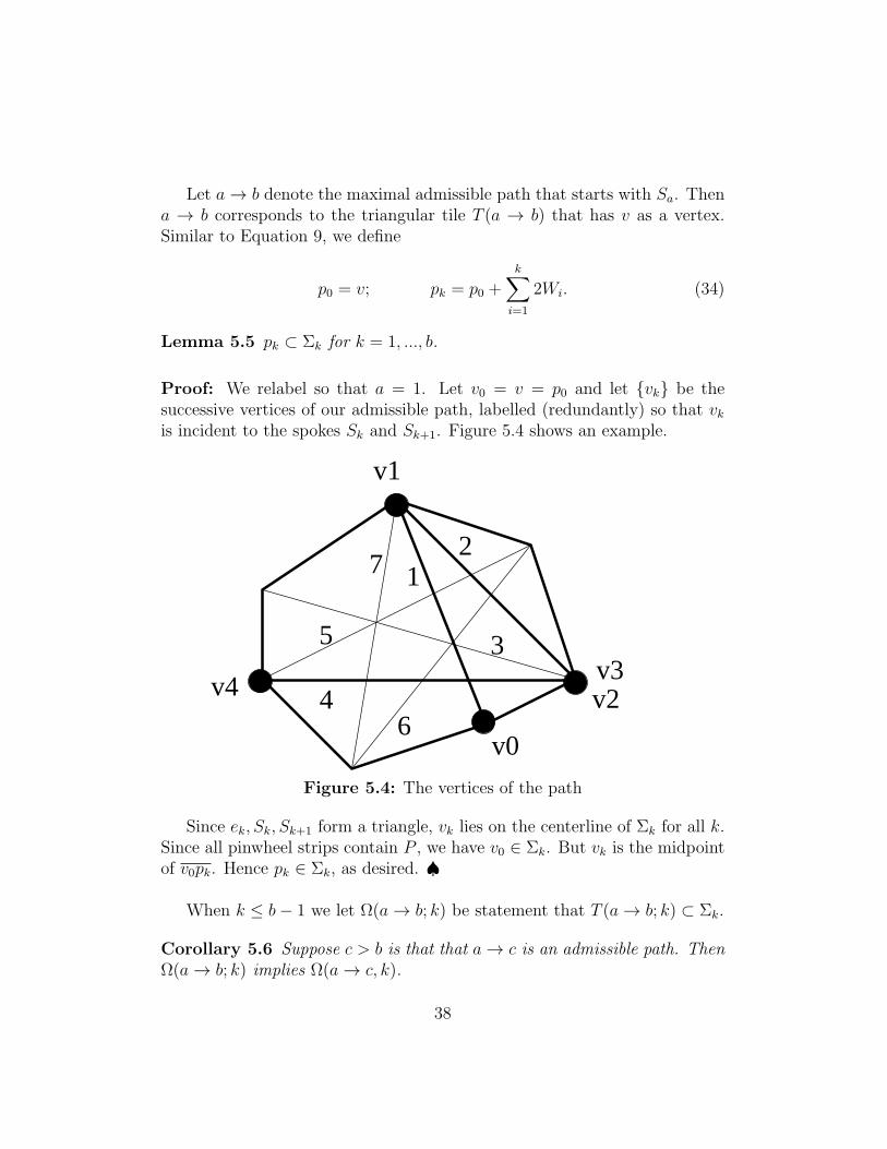
Let a→ b denote the maximal admissible path that starts with Sa. Thena → b corresponds to the triangular tile T (a → b) that has v as a vertex.Similar to Equation 9, we define

p0 = v; pk = p0 +k∑

i=1

2Wi. (34)

Lemma 5.5 pk ⊂ Σk for k = 1, ..., b.

Proof: We relabel so that a = 1. Let v0 = v = p0 and let vk be thesuccessive vertices of our admissible path, labelled (redundantly) so that vkis incident to the spokes Sk and Sk+1. Figure 5.4 shows an example.

2

5 3

7

64

1

v1

v2v3

v4

v0

Figure 5.4: The vertices of the path

Since ek, Sk, Sk+1 form a triangle, vk lies on the centerline of Σk for all k.Since all pinwheel strips contain P , we have v0 ∈ Σk. But vk is the midpointof v0pk. Hence pk ∈ Σk, as desired. ♠

When k ≤ b− 1 we let Ω(a→ b; k) be statement that T (a→ b; k) ⊂ Σk.

Corollary 5.6 Suppose c > b is that that a→ c is an admissible path. ThenΩ(a→ b; k) implies Ω(a→ c, k).

38

Proof: The admissible paths a→ b and a→ c agree except for possibly thelast edge of a→ b. Hence the sets

T (a→ b; k); T (a→ c; k); pk

are respectively translates, by the same vector X, of the sets

T (a→ b); T (a→ c); p0.

Let T (a → b) denote the convex hull of T (a → b) and p0. Let T (a → b; k)denote the convex hull of T (a→ b; k) and pk. First of all,

T (a→ c) ⊂ T (a→ b), (35)

by the analysis done in connection with Figure 4.2. Translating the wholepicture by X, we have

T (a→ c; k) ⊂ T (a→ b; k) ⊂ Σk. (36)

The second equality follows from the convexity of Σk. ♠

Corollary 5.6 is just a restatement of Property 3.

39

References

[D] R. Douady, These de 3-eme cycle, Universite de Paris 7, 1982.

[DF] D. Dolyopyat and B. Fayad, Unbounded orbits for semicircu-lar outer billiards , Annales Henri Poincare, to appear.

[DT1] F. Dogru and S. Tabachnikov, Dual billiards , Math. Intelli-gencer 26(4):18–25 (2005).

[DT2] F. Dogru and S. Tabachnikov, Dual billiards in the hyper-bolic plane, Nonlinearity 15:1051–1072 (2003).

[G] D. Genin, Regular and Chaotic Dynamics of Outer Billiards ,Pennsylvania State University Ph.D. thesis, State College (2005).

[GS] E. Gutkin and N. Simanyi, Dual polygonal billiard and neck-lace dynamics , Comm. Math. Phys. 143:431–450 (1991).

[Ko] Kolodziej, The antibilliard outside a polygon, Bull. Pol. AcadSci. Math. 37:163–168 (1994).

[M1] J. Moser, Is the solar system stable? , Math. Intelligencer 1:65–71(1978).

[M2] J. Moser, Stable and random motions in dynamical systems,with special emphasis on celestial mechanics , Ann. of Math. Stud. 77,Princeton University Press, Princeton, NJ (1973).

[N] B. H. Neumann, Sharing ham and eggs , Summary of a Manch-ester Mathematics Colloquium, 25 Jan 1959, published in Iota, theManchester University Mathematics Students’ Journal.

[S1] R. E. Schwartz, Unbounded Orbits for Outer Billiards , J. Mod.Dyn. 3:371–424 (2007).

[S2] R. E. Schwartz, Outer Billiards on Kites , Annals of Mathe-

40

matics Studies 171, Princeton University Press (2009)

[T1] S. Tabachnikov, Geometry and billiards , Student MathematicalLibrary 30, Amer. Math. Soc. (2005).

[T2] S. Tabachnikov, Billiards , Societe Mathematique de France,“Panoramas et Syntheses” 1, 1995

[VS] F. Vivaldi and A. Shaidenko, Global stability of a class of dis-continuous dual billiards , Comm. Math. Phys. 110:625–640 (1987).

41