Rutgers CS334

1

Digital Imaging and Multimedia

Filters

Ahmed Elgammal Dept. of Computer Science

Rutgers University

Outlines

  What are Filters   Linear Filters   Convolution operation   Properties of Linear Filters   Application of filters   Nonlinear Filter   Normalized Correlation and finding patterns in images   Sources:

  Burger and Burge “Digital Image Processing” Chapter 6   Forsyth and Ponce “Computer Vision a Modern approach”

Rutgers CS334

2

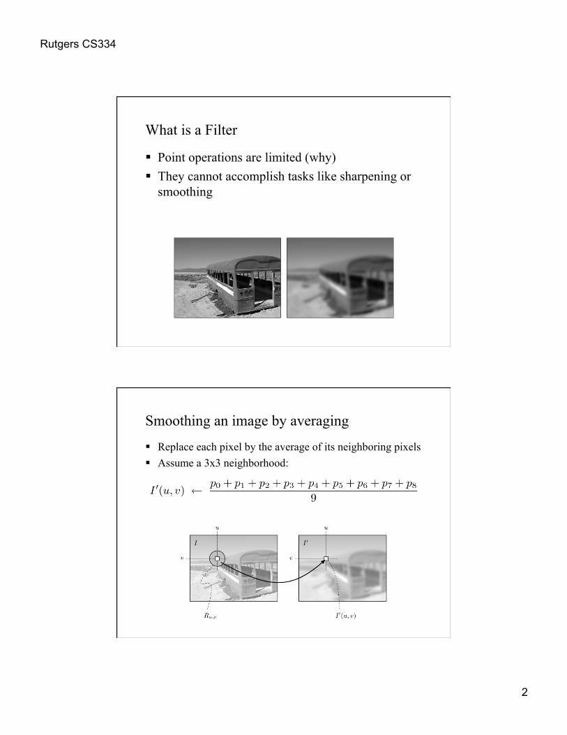
What is a Filter

  Point operations are limited (why)   They cannot accomplish tasks like sharpening or

smoothing

Smoothing an image by averaging

  Replace each pixel by the average of its neighboring pixels   Assume a 3x3 neighborhood:

Rutgers CS334

3

  In general a filter applies a function over the values of a small neighborhood of pixels to compute the result

  The size of the filter = the size of the neighborhood: 3x3, 5x5, 7x7, …, 21x21,..

  The shape of the filter region is not necessarily square, can be a rectangle, a circle…

  Filters can be linear of nonlinear

Rutgers CS334

4

Linear Filters: convolution

Averaging filter

Rutgers CS334

5

Types of Linear Filters

  Computing the filter operation   The filter matrix H moves over the original image I to compute the

convolution operation   We need an intermediate image storage!   We need 4 for loops!   In general a scale is needed to obtain a normalized filter.   Integer coefficient is preferred to avoid floating point operations

Rutgers CS334

6

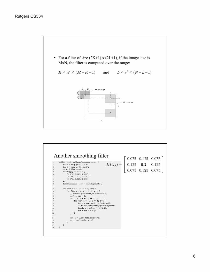
  For a filter of size (2K+1) x (2L+1), if the image size is MxN, the filter is computed over the range:

Another smoothing filter

Rutgers CS334

7

Integer coefficient

  Ex: linear filter in Adobe photoshop

Rutgers CS334

8

Mathematical Properties of Linear Convolution   For any 2D discrete signal, convolution is defined

as:

Properties

  Commutativity

  Linearity

(notice)   Associativity

Rutgers CS334

9

Properties

  Separability

Types of Linear Filters

Rutgers CS334

10

Smoothing by Averaging vs. Gaussian

Flat kernel: all weights equal 1/N

Smoothing with a Gaussian

  Smoothing with an average actually doesn’t compare at all well with a defocussed lens   Most obvious difference is

that a single point of light viewed in a defocussed lens looks like a fuzzy blob; but the averaging process would give a little square.

  A Gaussian gives a good model of a fuzzy blob

Rutgers CS334

11

  The picture shows a smoothing kernel proportional to

(which is a reasonable model of a circularly symmetric fuzzy blob)

An Isotropic Gaussian

Smoothing with a Gaussian

Rutgers CS334

12

Gaussian smoothing

  Advantages of Gaussian filtering   rotationally symmetric (for large filters)   filter weights decrease monotonically from central

peak, giving most weight to central pixels   Simple and intuitive relationship between size of σ and

the smoothing.   The Gaussian is separable…

Advantage of seperability

  First convolve the image with a one dimensional horizontal filter

  Then convolve the result of the first convolution with a one dimensional vertical filter

  For a kxk Gaussian filter, 2D convolution requires k2 operations per pixel

  But using the separable filters, we reduce this to 2k operations per pixel.

Rutgers CS334

13

Separability

2 3 3

3 5 5

4 4 6

1 2 1

1

2 1

18

11

18

18

11

18 65

1 2 1 1

2 1

1 2 1

2 4 2

1 2 1

2 3 3

3 5 5

4 4 6

=2 + 6 + 3 = 11

= 6 + 20 + 10 = 36

= 4 + 8 + 6 = 18

65

=

x

Advantages of Gaussians

  Convolution of a Gaussian with itself is another Gaussian   so we can first smooth an image with a small Gaussian   then, we convolve that smoothed image with another

small Gaussian and the result is equivalent to smoother the original image with a larger Gaussian.

  If we smooth an image with a Gaussian having sd σ twice, then we get the same result as smoothing the image with a Gaussian having standard deviation (2σ)

Rutgers CS334

14

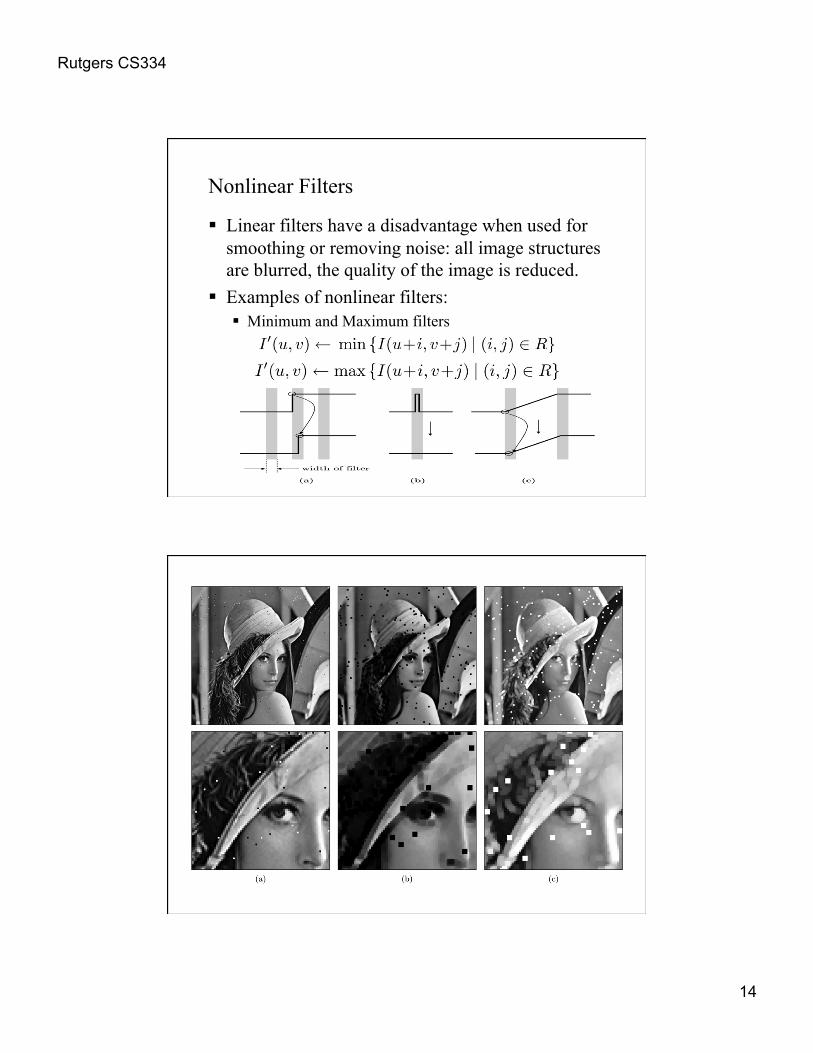
Nonlinear Filters

  Linear filters have a disadvantage when used for smoothing or removing noise: all image structures are blurred, the quality of the image is reduced.

  Examples of nonlinear filters:   Minimum and Maximum filters

Rutgers CS334

15

Median Filter

  Much better in removing noise and keeping the structures

Rutgers CS334

16

Weighted median filter

Linear Filters: convolution

Rutgers CS334

17

Convolution as a Dot Product

  Applying a filter at some point can be seen as taking a dot-product between the image and some vector

  Convoluting an image with a filter is equivalent to taking the dot product of the filter with each image window.

Original image Filtered image

Window

weights

weights

Window

  Largest value when the vector representing the image is parallel to the vector representing the filter

  Filter responds most strongly at image windows that looks like the filter.

  Filter responds stronger to brighter regions! (drawback) Insight:   filters look like the effects they are intended to find   filters find effects they look like

Ex: Derivative of Gaussian used in edge detection looks like edges

weights

Window

Rutgers CS334

18

Normalized Correlation   Convolution with a filter can be used to find templates in

the image.   Normalized correlation output is filter output, divided by

root sum of squares of values over which filter lies   Consider template (filter) M and image window N:

Original image Filtered image (Normalized Correlation

Result)

Window

Template

Normalized Correlation

  This correlation measure takes on values in the range [0,1]   it is 1 if and only if N = cM for some constant c   so N can be uniformly brighter or darker than the template,

M, and the correlation will still be high.   The first term in the denominator, ΣΣM2 depends only on

the template, and can be ignored   The second term in the denominator, ΣΣN2 can be

eliminated if we first normalize the grey levels of N so that their total value is the same as that of M - just scale each pixel in N by ΣΣ M/ ΣΣ N

Rutgers CS334

19

Positive responses

Zero mean image, -1:1 scale Zero mean image, -max:max scale

Positive responses

Zero mean image, -1:1 scale Zero mean image, -max:max scale

Rutgers CS334

20

Figure from “Computer Vision for Interactive Computer Graphics,” W.Freeman et al, IEEE Computer Graphics and Applications, 1998 copyright 1998, IEEE