Output-input stability and minimum-phase nonlinear … IEEE TRANSACTIONS ON AUTOMATIC CONTROL, VOL. 47, NO. 3, MARCH 2002 Output–Input Stability and Minimum-Phase Nonlinear Systems

422 IEEE TRANSACTIONS ON AUTOMATIC CONTROL, VOL. 47, NO. 3, MARCH 2002

Output–Input Stability and Minimum-PhaseNonlinear Systems

Daniel Liberzon, Member, IEEE, A. Stephen Morse, Fellow, IEEE, and Eduardo D. Sontag, Fellow, IEEE

Abstract—This paper introduces and studies the notion ofoutput–input stability, which represents a variant of the min-imum-phase property for general smooth nonlinear controlsystems. The definition of output–input stability does not rely ona particular choice of coordinates in which the system takes anormal form or on the computation of zero dynamics. In the spiritof the “input-to-state stability” (ISS) philosophy, it requires thestate and the input of the system to be bounded by a suitable func-tion of the output and derivatives of the output, modulo a decayingterm depending on initial conditions. The class of output–inputstable systems thus defined includes all affine systems in globalnormal form whose internal dynamics are input-to-state stableand also all left-invertible linear systems whose transmissionzeros have negative real parts. As an application, we explain howthe new concept enables one to develop a natural extension tononlinear systems of a basic result from linear adaptive control.

Index Terms—Adaptive control, asymptotic stabilization,detectability, input-to-state stability (ISS), minimum phase,nonlinear system, relative degree.

I. INTRODUCTION

A CONTINUOUS-TIME linear single-input–single-output(SISO) system is said to beminimum-phaseif the nu-

merator polynomial of its transfer function has all its zeros inthe open left half of the complex plane. This property can begiven a simple interpretation that involves therelative degreeof the system, which equals the difference between the degreesof the denominator and the numerator of the transfer function.Namely, if a linear system of relative degreeis minimum-phase, then the “inverse” system, driven by theth derivativeof the output of the original system, is stable. For left-invert-ible, multiple-input–multiple-output (MIMO) systems, in placeof the zeros of the numerator one appeals to the so-calledtrans-mission zeros[10].

The notion of a minimum-phase system is of great signifi-cance in many areas of linear system analysis and design. Inparticular, it has played an important role in parameter adaptivecontrol. A basic example is provided by the “certainty equiva-lence output stabilization theorem” [11], which says that when

Manuscript received June 9, 2000; revised March 26, 2001. Recommendedby Associate Editor W. Lin. The work of D. Liberzon was supported by theNational Science Foundation under Grant ECS-0114725. The work of A. S.Morse was supported by the Air Force Office of Scientific Research, DARPA,and the National Science Foundation. The work of E. D. Sontag was supportedby the U.S. Air Force under Grant F49620-98-1-0242.

D. Liberzon is with the Coordinated Science Laboratory, University of Illinoisat Urbana-Champaign, Urbana, IL 61801 USA (e-mail: [email protected]).

A. S. Morse is with the Department of Electrical Engineering, Yale Univer-sity, New Haven, CT 06520 USA (e-mail: [email protected]).

E. D. Sontag is with the Department of Mathematics, Rutgers University, NewBrunswick, NJ 08903 USA (e-mail: [email protected]).

Publisher Item Identifier S 0018-9286(02)02820-9.

a certainty equivalence, output stabilizing adaptive controlleris applied to a minimum-phase linear system, the closed-loopsystem is detectable through the tuning error. In essence, thisresult serves as a justification for the certainty equivalence ap-proach to adaptive control of minimum-phase linear systems.

For nonlinear systems that are affine in controls, a majorcontribution of Byrnes and Isidori [3] was to define the min-imum-phase property in terms of the new concept ofzero dy-namics.The zero dynamics are the internal dynamics of thesystem under the action of an input that holds the output con-stantly at zero. The system is calledminimum-phaseif the zerodynamics are (globally) asymptotically stable. In the SISO case,a unique input capable of producing the zero output is guaran-teed to exist if the system has a uniform relative degree, whichis now defined to be the number of times one has to differentiatethe output until the input appears. Extensions to MIMO systemsare discussed in [4] and [6].

In view of the need to work with the zero dynamics, the abovedefinition of a minimum-phase nonlinear system prompts oneto look for a change of coordinates that transforms the systeminto a certain normal form. It has also been recognized that justasymptotic stability of the zero dynamics is sometimes insuf-ficient for control design purposes, so that additional require-ments need to be placed on the internal dynamics of the system.One such common requirement is that the internal dynamics beinput-to-state stablewith respect to the output and its derivativesup to order , where is the relative degree (see, for instance,[13]). These remarks suggest that while the current notion ofa minimum-phase nonlinear system is important and useful, itis also of interest to develop alternative (and possibly stronger)concepts which can be applied when asymptotic stability of zerodynamics is difficult to verify or inadequate.

In this paper, we introduce the notion ofoutput–input sta-bility, which does not rely on zero dynamics or normal formsand is not restricted to affine systems. Loosely speaking, we willcall a system output–input stable if its state and input eventuallybecome small when the output and derivatives of the output aresmall. Conceptually, the new notion relates to the existing con-cept of a minimum-phase nonlinear system in much the sameway as input-to-state stability (ISS) relates to global asymptoticstability under zero inputs (0-GAS), modulo the duality betweeninputs and outputs. An important outcome of this parallelism isthat the tools that have been developed for studying ISS and re-lated concepts can be employed to study output–input stability,as will be discussed below.

It will follow from our definition that if a system hasa uniform relative degree (in an appropriate sense) and isdetectable through the output and its derivatives up to some

0018-9286/02$17.00 © 2002 IEEE

LIBERZON et al.: OUTPUT–INPUT STABILITY AND MINIMUM-PHASE NONLINEAR SYSTEMS 423

order, uniformly over all inputs that produce a given output,then it is output–input stable. For SISO systems that are realanalytic in controls, we will show that the converse is alsotrue, thus arriving at a useful equivalent characterization ofoutput–input stability (Theorem 1). We will prove that theclass of output–input stable systems as defined here includesall left-invertible linear systems whose transmission zeros havenegative real parts (Theorem 2) and all affine systems in globalnormal form with input-to-state stable internal dynamics.

Relying on a series of observations and auxiliary resultsdeduced from the new definition, we will establish a naturalnonlinear counterpart of the certainty equivalence outputstabilization theorem from linear adaptive control (Theorem 3).This conceptually important and intuitively appealing result didnot seem to be attainable within the boundaries of the existingtheory of minimum-phase nonlinear systems. It serves toillustrate that output–input stability is a reasonable and usefulextension of the notion of a minimum-phase linear system. Inview of the remarks made earlier, it is probable that the newconcept will find other applications in a variety of nonlinearcontrol contexts.

The proposed definition is precisely stated in the next section.In Section III, we give a somewhat nonstandard definition of rel-ative degree, which is especially suitable for subsequent devel-opments. In Section IV, we review the notions of detectabilityand ISS. In Section V, we study the output–input stability prop-erty with the help of the concepts discussed in Sections III andIV. In Section VI, we derive some useful results for cascadesystems. In Section VII, we present a nonlinear version of thecertainty equivalence output stabilization theorem. Section VIIIcontains some remarks on output–input stability of input–outputoperators. The contributions of the paper are briefly summarizedin Section IX. Examples are provided throughout the paper toillustrate the ideas.

II. DEFINITION AND PRELIMINARY REMARKS

We consider nonlinear control systems of the general form

(1)

where the state takes values in , the input takes valuesin , the output takes values in (for some positive inte-gers , , and ), and the functions and are smooth ( ).Admissible input (or “control”) signals are locally essentiallybounded, Lebesgue measurable functions .For every initial condition and every input , there is amaximally defined solution of the system (1), and the cor-responding output . Note that whenever the input function

is times continuously differentiable, whereis a posi-tive integer, the derivatives are well defined (thisissue will be addressed in more detail later).

Recall that a function is said to be ofclass if it is continuous, strictly increasing, and .If is unbounded, then it is said to be ofclass . Afunction is said to be ofclass

if is of class for each fixed anddecreases to 0 as for each fixed .

We will let denote the essential supremumnorm of a signal restricted to an interval , i.e.,

, whereis the standard Euclidean norm. When some vectors

are given, we will often usethe simplified notation for the “stack” vector

. Given an -valued signaland a nonnegative integer, we will denote by the

-valued signal

provided that the indicated derivatives exist.We are now in position to introduce the main concept of this

paper.Definition 1: We will call the system (1)output–input stable

if there exist a positive integer , a class function , anda class function such that for every initial state andevery times continuously differentiable input the in-equality

(2)

holds for all in the domain of the corresponding solution of(1).

The inequality (2) can be interpreted in terms of two separateproperties of the system. The first one is that if the output andits derivatives are small, then the input becomes small. Roughlyspeaking, this means that the system has a stable left inversein the input–output sense. However, no explicit construction ofsuch a left inverse is necessary. The second property is thatif the output and its derivatives are small, then the state be-comes small. This signifies that the system is (zero-state) de-tectable through the output and its derivatives, uniformly withrespect to inputs1; we will call such systems “weakly uniformly0-detectable” (see Section IV). Thus output–input stable sys-tems form a subclass of weakly uniformly 0-detectable ones.Detectability is a state-space concept, whose attractive featureis that it can be characterized by Lyapunov-like dissipation in-equalities.

In view of the bound on the magnitude of the state, a morecomplete name for the property introduced here would perhapsbe “(differential) output-to-input-and-state stability” (DOSIS),but we choose to call it output–input stability for simplicity. Theconditions imposed by Definition 1 capture intrinsic propertiesof the system, which are independent of a particular coordinaterepresentation. They are consistent with the intuition providedby the concept of a minimum-phase linear system. In fact, forSISO linear systems the output–input stability property reducesprecisely to the classical minimum-phase property, as we nowshow.

Example 1: Consider a stabilizable and detectable linearSISO system

(3)

1In particular, this detectability property is preserved under state feedback; forcomparison, recall that every minimum-phase linear system is detectable underall feedback laws.


Let be its relative degree. This means that we havebut . From the

formula we immediately obtain

(4)

Moreover, it is well known that there exists a linear change ofcoordinates , where , , and ,which transforms the system (3) into the normal form

and (3) is minimum-phase (in the classical sense) if and onlyif is a stable matrix. Stability of is equivalent to the exis-tence of positive constantsand such that for all initial statesand all inputs we have (it isalso equivalent to detectability of the transformed system withextended output ). Combining the last inequality with(4), we arrive at

This yields (2) with . On the other hand, if (2) holds,then we know that implies , and so (3) mustbe minimum-phase. Thus we see that for stabilizable and de-tectable linear SISO systems, output–input stability is equiv-alent to the usual minimum-phase property. Incidentally, notethat when in (2), the smoothness of becomes super-fluous, because is automatically times (almost everywhere)differentiable for every admissible input.

The above remarks suggest that the concepts of relative de-gree and detectability are related to the output–input stabilityproperty. In the subsequent sections, we will develop some ma-chinery which is needed to study this relationship, and exploreto what extent the situation described in Example 1 carries overto (possibly MIMO) nonlinear systems.

We conclude this section with another motivating observa-tion, important from the point of view of control design. It isformally expressed by the following proposition.

Proposition 1: Assume that the system (1) is output–inputstable. Suppose that we are given a feedback law withthe following properties: there exists a system:

(5)

with a globally asymptotically stable equilibrium at the origin, asmooth map with , and a class func-tion such that for every initial condition for the system

(6)

there exists an initial condition for the system (5) withfor which we have

along the corresponding solutions. Then the origin is a globallyasymptotically stable equilibrium of the closed-loop system (6).

Proof: Global asymptotic stability of the system (5) is ex-pressed by the inequality

(7)

for some . Under the action of the control law ,the output of the system (1) satisfies (omitting time dependence)

, , and so on. Using the standingassumptions on and , it is straightforward to verify that forsome class function we have , where

is the integer that appears in Definition 1. Combined with (7),this gives

(8)

Using (2), global asymptotic stability of the closed-loop systemcan now be established by standard arguments (see Section VIfor details).

As an example, consider an affine system given by

(9)

Suppose that this system has a uniform relative degree(in thesense of [6]) and is output–input stable. It may or may not havea global normal form (construction of a global normal form re-quires additional properties besides relative degree [6]). How-ever, relabeling as , we have

where and . We can thenapply a state feedback law which brings this to the form

, where the last system has a globally asymptotically stableequilibrium at the origin. [One possible choice is a linearizingfeedback

where the numbers , are such that the poly-nomial has all its roots inthe left half-plane.] In view of Proposition 1, the entire systembecomes globally asymptotically stable [it is easy to constructa suitable function using the formulas ,

, and so on]. Note that this is true foreverysuch feedback law, which for minimum-phase systems is gener-ally not the case and special care needs to be taken in designinga stabilizing feedback (see [6, Sec. 9.2]).


III. RELATIVE DEGREE

A. SISO Systems

Let us first consider the case when the system (1) is SISO, i.e.,when . To specify what will be meant by “relativedegree,” we need to introduce some notation. Fordefine, recursively, the functions by theformulas and

(10)

where the arguments of are . As an illus-tration, in the special case of the SISO affine system (9) wehave and

(omitting the argumentin the directional derivatives).The significance of the functions lies in the fact that if

the input is in for some positive integer, then alongeach solution of (1) the corresponding output has a contin-uous th derivative satisfying

In particular, suppose that is independent offor all less than some positive integer. Then dependsonly on and , as given by

As an example, for the affine system (9) we have

(11)

In this case we see that for every initial condition and everyinput, exists and is an absolutely continuous function oftime, and we have

for almost all in the domain of the corresponding solution. Theconverse is also true, namely, if exists and is absolutelycontinuous for all initial states and all inputs, then must beindependent of for all . Indeed, if werea nonconstant function of for some , then it would takedifferent values at and for someand . Choosing the initial state andapplying the input for andfor , where is small enough, would produce an outputwith a discontinuous th derivative, contradicting the existenceand absolute continuity of .

Definition 2: We will say that a positive integeris the (uni-form) relative degreeof the system (1) if the following two con-ditions hold:

1) for each , the function is independent of;

2) there exist two class functions and such that

(12)

for all and all .

If there exists such an integer, then it is unique. This can bededuced from the following simple observation, which will alsobe needed later.

Remark 1: If Properties 1 and 2 in Definition 2 hold for somepositive integer , then there does not exist an such that

for all , where is some constant. [Indeed,otherwise we would have for all , acontradiction.]

We conclude that if some satisfies Definition 2, thencannot be independent of by virtue of Remark 1, hence prop-erty 1 in Definition 2 cannot hold for any . In view of theprevious remarks, is the relative degree of (1) if and only if forsome functions , for every initial condition, andevery input, exists and is absolutely continuous [hence,

exists almost everywhere] and the inequality

(13)

holds for almost all [to see why (13) implies (12), simply applyan arbitrary constant control ]. We next show that foraffine systems the above definition is consistent with the usualone.

Proposition 2: Consider the affine system (9). A positive in-teger is the relative degree of (9) in the sense of Definition 2 ifand only if for all and all integers ,

for all , and .Proof: Suppose that is the relative degree of (9) in the

sense of Definition 2. Applying (11) repeatedly, we see thatProperty 1 in Definition 2 implies for all .Moreover, if there were some with, then we would have which is in-

dependent of , contrary to Remark 1. Now, setting, we have , and so (12)

implies that must be 0 hence .Conversely, suppose thatsatisfies the properties in the state-

ment of the proposition. Then property 1 in Definition 2 is ver-ified using (11). Moreover, takes the form

, where and .Since for all and , we have

for some class functions and . If follows that:

from which property 2 in Definition 2 can be easily shown tohold.

Proposition 2 implies, in particular, that for the SISO affinesystem (9) with Definition 2 reduces to the standarddefinition of uniform relative degree as given, e.g., in the bookby Isidori [6] [simply note that implies ].Of course, the definition of relative degree proposed here is notrestricted to affine systems. As a simple example, the system

has relative degree 1 according to Definition 2. Thiscase is also covered by the definition of relative degree for notnecessarily affine systems given in [12, p. 417]. In general, how-


ever, our definition is more restrictive; for example, the systemwould have relative degree 1 in the context of

[12], but the bound (12) does not hold.Remark 2: The relative degree cannot exceed the dimension

of the system, i.e., if exists, then we must have . Forthe affine system (9), this is an immediate consequence of [6,Lemma 4.1.1] or [16, Corollary 5.3.8], which imply that ifisthe relative degree, at least locally at some , then therow vectors are linearly in-dependent in a neighborhood of in [so the functions

qualify as a partial set of newlocal coordinates]. For the general system (1), we can considerthe associated affine system

(14)

of dimension . If is the relative degree of (1), then thereexists a point at which (14) has relative degree

(in the sense of [6]). The results just mentioned then implythat the functions can serve as in-dependent coordinates in a neighborhood of in ,hence .

To prove one of our main results (Theorem 1 in Section V)we will need the following characterization of relative degree,which also has intrinsic interest.

Proposition 3: A positive integer is the relative degree of(1) if and only if the following three conditions are satisfied:

1) for each , the function is independent of;

2) for each compact set and each positive constant, there exists a number such that

whenever and ;3) for all .This in turn requires the following lemma, which is a simple

exercise on functions. Its proof is included for complete-ness.

Lemma 1: If a continuous function , whereis a positive integer, is such that when, and when , then there exists a class

function such that for all .Proof of Lemma 1:Consider the function

given by . This function is welldefined (because is radially unbounded so the minimum istaken over a compact set), continuous, positive definite, nonde-creasing, and unbounded, and we have for all .Then one can find a function such that (for arbi-trary such that is increasing on and con-stant on , let for ,and on let be linear with ). We have

, hence with .Proof of Proposition 3: Condition 1 in the statement of the

proposition exactly matches property 1 in Definition 2. If prop-erty 2 in Definition 2 holds, then condition 2 of the propositionis satisfied with . It isclear that property 2 in Definition 2 implies condition 3 of theproposition. It remains to show that conditions 2 and 3 of the

proposition imply property 2 in Definition 2. Let ,and consider the function . We claimthat this function satisfies the hypotheses of Lemma 1. Indeed,take an arbitrary . Condition 2 of the proposition im-plies that there exists an such that when-ever and . It follows that if

. Therefore, is radially unbounded. In viewof condition 3 of the proposition, clearly if .Thus we can apply Lemma 1, which guarantees the existence ofa function such that

From this, (12) follows with .

B. MIMO Systems

The above concept extends in a straightforward fashion to thecase when the system (1) is MIMO, i.e., whenand are notnecessarily equal to 1. For each , let be the thcomponent of , and define the functions ,

recursively by the formula (10) withinstead of . We will say that a set of positive integers

is a (uniform)relative degreeof the system (1) ifthe following two conditions hold:

1) for each and each , the functionis independent of ;

2) there exist two class functions and such that

for all and all .Similarly to the SISO case, is the relative degreeof (1) if and only if for some functions , for every

, every initial condition, and every input,exists and is absolutely continuous [hence exists almosteverywhere] and the inequality

holds for almost all. Using the same type of argument as in theproof of Proposition 2, one can show that for the square ( )affine system

with this reduces to the definition of uniform vectorrelative degree given in [6], which says that we must have

for all and all integers ,, , and that the matrix

defined by

must be nonsingular for all. More generally, for thecorresponding matrix must be left-invertible (i.e., of rank

) for all . Note that for MIMO systems the relative degree is


not necessarily unique (example: , ;is a relative degree for every ). Proposition 3 carries overto the MIMO setting subject to an obvious change of notation,but this will not be needed in the sequel.

IV. DETECTABILITY AND RELATED NOTIONS

Consider a general system of the form

We recall from [15] that this system is called input-to-statestable if there exist some functions andsuch that for every initial state and every input thecorresponding solution satisfies the inequality

for all . Intuitively, this means that the state eventuallybecomes small when the input is small.

Given a system with both inputs and outputs

(15)

we will say that it is0-detectableif there exist some functionsand such for every and every the

corresponding solution satisfies the inequality

as long as it exists. In particular, a system without inputs givenby

will be called0-detectableif there exist some functionsand such that for every initial state the corre-sponding solution satisfies the following inequality as long as itexists:

(16)

These concepts were studied in [17] under the names ofinput–output-to-state stabilityand output-to-state stability,respectively. In this paper we use the term “0-detectability” asa shorthand.

Let us call the system (15)uniformly 0-detectableif thereexist some functions and such that forevery initial state and every input the inequality (16)holds along the corresponding solution. As the name sug-gests, uniform 0-detectability amounts to 0-detectability thatis uniform with respect to inputs. This property was calleduniform output-to-state stabilityin [7] (see also [8]) andstrongdetectabilityin [5].

When working with output derivatives, it is helpful to intro-duce an auxiliary system whose output contains derivatives ofthe output of the original system (restricting admissible inputs ifnecessary to ensure that these derivatives are well defined). Wefirst describe this construction for SISO systems. Consider the

system (1) with . Take a nonnegative integer. Re-stricting the input to be in , we can consider the-outputextensionof (1):

(17)

where

is the new output map (here we are using the notation of Sec-tion III). That is, we redefine the output of the system to be.Of course, for we recover the original system. Note thatthe differentiability assumption oncan be relaxed if the func-tion is known to be independent of for allbetween 0 and some positive integer (cf. Section III). We willview (17) as a system whose input consists ofand all deriva-tives of that appear as arguments in the output map. Withsome abuse of terminology, we will apply to such systems thedefinitions of 0-detectability and uniform 0-detectability givenearlier. Let us call the system (1)weakly 0-detectable of order

if its -output extension (17) is 0-detectable. Also, let us callthe system (1)weakly uniformly 0-detectable of orderif its

-output extension (17) is uniformly 0-detectable.Now, consider the general MIMO case, i.e., take the system

(1) with and . For arbitrary nonnegative numbers, we can redefine the output of the system to be

restricting the input to be sufficiently smooth so that the indi-cated derivatives exist. This amounts to considering the system

(18)

where and

(in the notation of Section III). Similarly to the SISO case, wewill call this system the -output extensionof (1).We will say that the system (1) isweakly 0-detectable of order

if its -output extension (18) is 0-de-tectable. We will also say that the system (1) isweakly uniformly0-detectable of order if its -outputextension (18) is uniformly 0-detectable.

Another definition, which will be needed in Section VII, is thefollowing one (introduced in [18]). The system (15) is said to beinput-to-output stableif there exist some functions and

such that for every and every the followinginequality holds along the corresponding solution:


Finally, we remark that since all the systems under consid-eration are time-invariant, the same properties would result ifwe used an arbitrary initial time instead of 0 in the above in-equalities (changing the second argument offrom toaccordingly). This fact will be used implicitly in the proofs inSection VI.

V. OUTPUT–INPUT STABILITY

A. SISO Systems

We first study the SISO case, represented by the system (1)with . Our main result in this section is the followingcharacterization of output–input stability for SISO systems.

Theorem 1:

1) Suppose that the system (1) has a relative degreein thesense of Definition 2 and is weakly uniformly 0-detectableof order , for some . Then (1) is output–input stable in thesense of Definition 1, with .

2) Suppose that the system (1) is output–input stable in thesense of Definition 1. Then it is weakly uniformly 0-de-tectable of order .

3) Suppose that the system (1) is output–input stable in thesense of Definition 1, that the function is real an-alytic in for each fixed , and that and

. Then (1) has a relative degree in the senseof Definition 2.

The theorem implies that for systems with relative degree,output–input stability is equivalent to weak uniform 0-de-tectability of order for some , and that for systemssatisfying the additional assumptions onand stated inpart 3, output–input stability is equivalent to the existence ofa relative degree plus weak uniform 0-detectability oforder for some .

Proof: Part 1. Since is the relative degree, the inequality(13) holds with . Suppose that for some thesystem (1) is weakly uniformly 0-detectable of order. Thiscan be expressed as

where and (see Section IV). Combiningthis with (13) and using the simple fact that for every classfunction and arbitrary numbers one has

, we arrive at the inequality (2) with, , and

. Thus (1) is output–input stable asneeded.

Part 2. Follows immediately from the definitions.Part 3. Since the system (1) is output–input stable, we know in

particular that for some positive integer and some functionsand the inequality

(19)

holds along solutions of (1) for all smooth inputs. The func-tion cannot be independent of for all

. Otherwise, letting and applying an arbi-trary constant input , we would deduce from (19) that

, a contradiction. Thus, the in-teger

is independent of

(20)

is well defined. Condition 1 of Proposition 3 holds with this.For every input we have

(21)

The following fact will be useful.Lemma 2: If (19) holds and is defined by (20), then

there cannot exist a bounded sequence in , a se-quence in with , and a positiveconstant such that for all we have and

.Proof: Suppose that there exist sequences and

and a positive constant with the properties indicated in thestatement of the lemma. Fix an arbitrary positive integer. Con-sider the initial state , and pick a smooth (e.g., poly-nomial) input function with whose derivativesat are specified recursively by the equations

(22)

In view of (21), we will then have

Therefore, if such an input is applied and if is an arbitraryfixed positive number, then there exists a sufficiently small time

such that for all the following inequalities hold:


Repeating this construction for all, we obtain a sequence oftrajectories of (1) along which , areuniformly bounded for small, whereas is unboundedfor small and large . We arrive at a contradiction with (19),and the proof of the lemma is complete.

Let us denote by the set of all such that is aconstant function. The set is closed [because if for a sequence

converging to some we havefor all and all , then for all ].

Lemma 3: Suppose that is real analytic in for eachfixed , that (19) holds, and thatis defined by (20). Ifis such that for some we have for all ,then is in the interior of .

Proof: Take an arbitrary sequence in with. By hypothesis, for all .

By continuity, for each there exist a neighborhood ofin and a positive number such that

for all and all . Moreover,the neighborhoods , can be chosen to benested, i.e., whenever , and the sequence

can be chosen to be nonincreasing. Now, suppose thatisnot in the interior of . Fix an arbitrary . We have .Take an arbitrary . Thencannot be identically zero on the interval ,by virtue of real analyticity of which follows fromthat of . Thus, we can find asuch that . This construction can becarried out for all . Since when , thepoints , can be chosen in such a way that isuniformly bounded for all . Moreover, we have

as . In view of Lemma 2, wearrive at a contradiction with (19), which proves the lemma.

Corollary 1: Suppose that is real analytic in foreach fixed . If (19) holds and is defined by (20), then the set

is open.Proof: By definition of , every satisfies the con-

dition in the statement of Lemma 3, hence it lies in the interiorof .

Corollary 2: Suppose that is real analytic in foreach fixed . If (19) holds and is defined by (20), then the set

is empty.Proof: We know that is closed. We also know that

is open (Corollary 1). Moreover, by virtue of (20).Being a closed and open proper subset of, the set must beempty.

Our goal is to show that Conditions 2 and 3 of Proposition 3hold, which would imply that is the relative degree of (1). Webreak this into two separate statements.

Lemma 4: Suppose that is real analytic in for eachfixed . If (19) holds and is defined by (20), then for eachcompact set and each positive constant there existsa number such that whenever and

.Proof: Suppose that, contrary to the statement of the

lemma, there exist a compact subset of , a positiveconstant , a sequence in , and a sequence in

with such that forall . By continuity, we can find a nonincreasing sequence of

positive numbers such that for alland all . Fix an arbitrary . Sinceis empty by Corollary 2 and is real analytic,

cannot vanish identically on the interval. Thus, we can find a

such that . Repeat this constructionfor all . Lemma 2 applies again, yielding a contradiction with(19), and the proof of the lemma is complete.

Lemma 5: Suppose that is real analytic in for eachfixed and that we have and . If (19) holdsand is defined by (20), then for all .

Proof: Suppose that for some . Weknow from Corollary 2 that the set is empty. Thus, by real ana-lyticity cannot vanish identically on any openneighborhood of . This implies that there exists a sequence

converging to such that [if, simply let ]. Choose an ar-

bitrary . Take the initial state to be . Pick a smooth(e.g., polynomial) input function such thatand (22) holds with 0 in place of . From (21), we immedi-ately see that . Since ,we have . We also know that , whichimplies that . It follows that

. We conclude that if the inputis applied, then for every there exists a sufficiently

small time such that for all the following inequal-ities hold:

Carrying out the above construction for all and notingthat , we see that

become arbitrarily small for smallas . On the other hand, , sois bounded away from 0 for small and large . This is acontradiction with (19), which proves the lemma.

We have shown that the integerdefined by (20) satisfies allthree conditions of Proposition 3, thusis the relative degree ofthe system (1). This proves part 3, and the proof of Theorem 1is complete.

As an illustration, consider the affine system (9) with. Its right-hand side is obviously real analytic in. Recon-

structing the above proof for this case, we find thatis thesmallest integer for which is not identically zeroon , and . If the system isoutput–input stable, then Corollary 2 implies thatmust beempty, which means that is the relative degree (see Proposi-tion 2). Since the hypothesis is only used in Lemma5, it is not needed in this case.

We will be especially interested in systems that are coveredby Part 1 of Theorem 1 with . We give such systemsa separate name to emphasize the relationship with the existingterminology (which will be explained in the next example). Notethat is a function of the state only: ; nodifferentiability assumptions need to be placed on.


Definition 3: Let us call the system (1)strongly minimum-phaseif it has a relative degreeand is weakly uniformly 0-de-tectable of order .

Example 2: Consider an affine system in global normal form

(23)

where , , and(so that is the uniform relative degree by Proposition 2). Thissystem is usually called minimum-phase if thezero dynamics

have an asymptotically stable equilibrium at(see [3]). Since , the above definition of the strongminimum-phase property in this case demands that the equa-tion for in (23), which represents the internal dynamics, beISS with respect to (more precisely, with respect to all pos-sible signals that can be generated by the-subsystem). Thisis, in general, a stronger condition than just asymptotic stabilityof the zero dynamics; however, in the linear case the two prop-erties are equivalent (and both amount to saying that all zeros ofthe transfer function must have negative real parts). As we al-ready mentioned, the ISS assumption has been imposed on theinternal dynamics of the system in various contexts associatedwith control design (see, e.g., [13]).

Remark 3: The bound (13), which is a consequence of ourdefinition of relative degree, does not necessarily imply that onecan explicitly solve for in terms of and (“flatness”);example: . However, this is possible for some systems,in particular, it can always be done for the affine system (9). Inthis case, we can expressas a function of and ,where is an arbitrary stable polynomial of degreeand

. Substituting this expression for, we obtain an “inverse”system, driven by . If the system (1) is strongly minimum-phase, then it is not hard to show that this inverse system willbe ISS with respect to. For example, consider the system inglobal normal form (23). Take a stable polynomial

, and rewrite the equation for as. Then the -dimensional

subsystem that describes the evolution ofis easily seen to be astable linear system driven by, hence it is ISS with respect to. If the system is ISS with respect to (recall that

this is a consequence of the strong minimum-phase property)then the overall system is indeed ISS with respect to, becausea cascade of two ISS systems is ISS.

The results of [8] and [17] imply that the system (1) is weaklyuniformly 0-detectable of order if there exists a smooth,positive—definite, radially unbounded functionthat satisfies

(24)

for some functions . This Lyapunov-like dissipa-tion inequality can be used to check the strong minimum-phase

property, once the relative degree of the system is known. Wesummarize this observation in the following statement.

Proposition 4: Suppose that the system (1) has a relative de-gree and that for some smooth, positive definite, radially un-bounded function and class functions theinequality (24) holds. Then (1) is strongly minimum-phase.

In fact, (24) provides a necessary and sufficient condition forweak uniform 0-detectability of order if controls takevalues in a compact set [8]. Unfortunately, this condition is onlysufficient and not necessary if the control set is unbounded. Forexample, consider the integrator , . It is obvi-ously uniformly 0-detectable (here ), but for every smoothpositive–definite and every in the nonempty set

the quantity can be made arbi-trarily large by a suitable choice of.

Of course, the inequality (24) with instead of canbe applied to check weak uniform 0-detectability of order,as long as is well defined. A similar recipe for finding therelative degree with the help of Lyapunov-like functions doesnot seem to exist. However, for many systems of interest it isnot difficult to verify the existence of relative degree directly byusing Definition 2 or Proposition 3.

Example 3: We now give an example of an output–inputstable system that is not strongly minimum-phase. Consider thesystem

(25)

It has relative degree 1. From the equation ,which is ISS with respect to, we see that the system (25) isweakly uniformly 0-detectable of order 1. Therefore, (25) isoutput–input stable (with ) by virtue of part 1 of The-orem 1. Now let us show that this system is not strongly min-imum-phase, i.e., it is not uniformly 0-detectable (with respectto the original output ). It is enough to find a solution trajectoryalong which converges to zero while does not converge tozero. Take the initial state to be 0, and apply the following input:

for , for ,for , for , for

, and so on. Then , whereas for wehave so .

The situation in the above example is dual to the one de-scribed in [1], where it is shown that ISS with respect to inputsand their derivatives is in general not equivalent to the usual ISS.

B. MIMO Systems

We now turn to the general case of (1) with and. The next result is readily obtained by the same argu-

ments as those employed in the proof of Theorem 1. We willsee below that the nontrivial part of Theorem 1, which statesthat under suitable assumptions output–input stability impliesthe existence of a relative degree, does not hold for MIMO sys-tems. We will also explain why this is an advantage, rather thana drawback, of our definition.


Proposition 5: Suppose that the system (1) has a relative de-gree . Then it is output–input stable, with

, if and only if it is weakly uniformly 0-de-tectable of order for some .

Of special interest are systems satisfying the condition ofProposition 5 with , . Accordingly,let us call the system (1)strongly minimum-phaseif it has a rel-ative degree and is weakly uniformly 0-detectableof order . Note that is a func-tion of only, as given by ,and no differentiability assumptions need to be placed on. Wethus obtain a generalization to MIMO systems of the strong min-imum-phase property introduced in the previous subsection. Ithas a similar interpretation in terms of input-to-state stability ofthe internal dynamics for systems in global normal form, andadmits an analogous Lyapunov-like sufficient condition.

However, we remark that for MIMO systems the existence ofa relative degree is quite a restrictive assumption. For example,linear systems with relative degree form a rather special subclassof those linear systems for which the minimum-phase property(in its classical sense) is well defined.2 Fortunately, Definition 1does not have the shortcoming of applying only to systems withrelative degree, as illustrated by the following example.

Example 4: The system

does not have a relative degree. This system is output–inputstable, as can be seen from the formulas

, , and the fact that the equationfor is ISS with respect to .

The above example is to be contrasted with the next one.Example 5: The system

does not have a relative degree. The zero dynamics of thissystem are , and the input that produces them isidentically zero. However, it can be shown by the same kindof argument as the one used in the proof of Theorem 1 thatarbitrarily large can lead to arbitrarily small , , andderivatives of . Therefore, this system is not output–inputstable.

We will now establish an important feature of Definition 1,namely, that for linear MIMO systems it reduces exactly to theclassical definition of the minimum-phase property. We will

2Basically, the reason for this is that the relative degree of a MIMO system canbe lost or gained as a result of a linear coordinate transformation in the outputspace, while the minimum-phase property is invariant under such transforma-tions.

make use of some concepts and results from the linear geometriccontrol theory (see [10] and [19]). Consider the linear system

(26)

with , , and . We assume that (26) is leftinvertible. Recall that a subspaceof is called -in-variantif there exists an matrix such that

. Denote by the family of all -invariant subspaces thatare contained in . Then has a unique largest member(with respect to inclusion) which we denote by. The eigen-values of the restriction of to are the same for all

such that . These eigenvalues are called thetransmission zerosof the system (26). Left-invertible linear sys-tems are usually called minimum-phase if all their transmissionzeros have negative real parts. Our goal is to prove that this isequivalent to the output–input stability property in the sense ofDefinition 1.

As a direct consequence of Silverman’s “structure algorithm”[14], there exists an -vector , whose components are linearcombinations of the components of and their derivatives,which satisfies

where the matrix is nonsingular. From this, we immediatelyobtain

An -vector of complementary coordinates can bechosen whose dynamics are independent of, as given by

. Consider the feedback matrix . Then isprecisely the largest -invariant subspace in ,and thus equals the unobservable subspace of ,i.e., . It follows that there ex-ists a linear change of coordinates such that

, and the components of are linear combi-nations of the components ofand their derivatives. In thesecoordinates, (26) takes the form

Its transmission zeros are the eigenvalues of. Reasoning ex-actly as in Example 1, we see thatis a stable matrix if andonly if the system is output–input stable. We summarize this asfollows.

Theorem 2: A left-invertible linear system is output–inputstable if and only if all its transmission zeros have negative realparts.

VI. CASCADE RESULTS

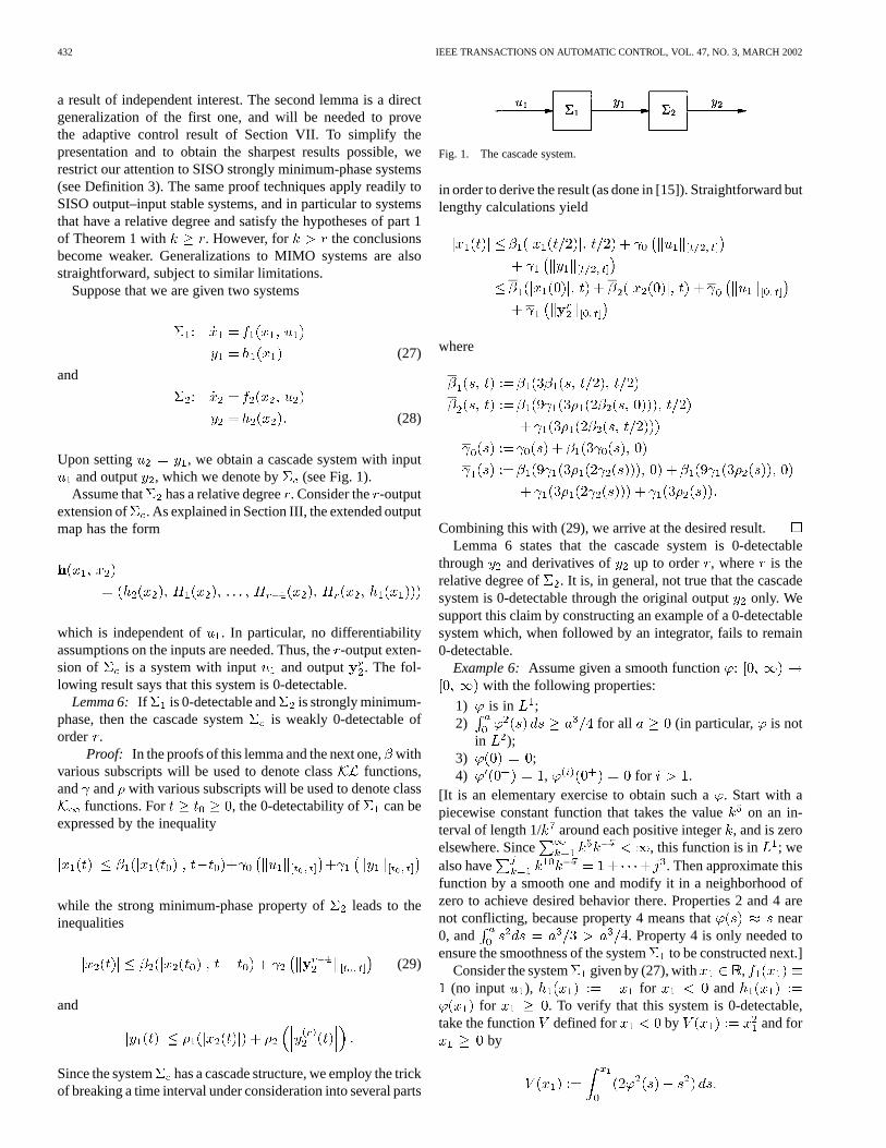
The purpose of this section is to investigate how theoutput–input stability property behaves under series connec-tions of several subsystems. We will prove two lemmas. Thefirst one says that the cascade of a 0-detectable system withan output–input stable system is weakly 0-detectable (i.e.,0-detectable through the output and its derivatives), which is


a result of independent interest. The second lemma is a directgeneralization of the first one, and will be needed to provethe adaptive control result of Section VII. To simplify thepresentation and to obtain the sharpest results possible, werestrict our attention to SISO strongly minimum-phase systems(see Definition 3). The same proof techniques apply readily toSISO output–input stable systems, and in particular to systemsthat have a relative degree and satisfy the hypotheses of part 1of Theorem 1 with . However, for the conclusionsbecome weaker. Generalizations to MIMO systems are alsostraightforward, subject to similar limitations.

Suppose that we are given two systems

(27)

and

(28)

Upon setting , we obtain a cascade system with inputand output , which we denote by (see Fig. 1).

Assume that has a relative degree. Consider the-outputextension of . As explained in Section III, the extended outputmap has the form

which is independent of . In particular, no differentiabilityassumptions on the inputs are needed. Thus, the-output exten-sion of is a system with input and output . The fol-lowing result says that this system is 0-detectable.

Lemma 6: If is 0-detectable and is strongly minimum-phase, then the cascade systemis weakly 0-detectable oforder .

Proof: In the proofs of this lemma and the next one,withvarious subscripts will be used to denote class functions,and and with various subscripts will be used to denote class

functions. For , the 0-detectability of can beexpressed by the inequality

while the strong minimum-phase property of leads to theinequalities

(29)

and

Since the system has a cascade structure, we employ the trickof breaking a time interval under consideration into several parts

Fig. 1. The cascade system.

in order to derive the result (as done in [15]). Straightforward butlengthy calculations yield

where

Combining this with (29), we arrive at the desired result.Lemma 6 states that the cascade system is 0-detectable

through and derivatives of up to order , where is therelative degree of . It is, in general, not true that the cascadesystem is 0-detectable through the original outputonly. Wesupport this claim by constructing an example of a 0-detectablesystem which, when followed by an integrator, fails to remain0-detectable.

Example 6: Assume given a smooth functionwith the following properties:

1) is in ;2) for all (in particular, is not

in );3) ;4) , for .

[It is an elementary exercise to obtain such a. Start with apiecewise constant function that takes the valueon an in-terval of length 1/ around each positive integer, and is zeroelsewhere. Since , this function is in ; wealso have . Then approximate thisfunction by a smooth one and modify it in a neighborhood ofzero to achieve desired behavior there. Properties 2 and 4 arenot conflicting, because property 4 means that near0, and . Property 4 is only needed toensure the smoothness of the systemto be constructed next.]

Consider the system given by (27), with ,(no input ), for and

for . To verify that this system is 0-detectable,take the function defined for by and for

by


The function is radially unbounded and positive definite [be-cause for we have using property 2 of ].Its derivative equals for andfor . Thus we have for all

. In view of the results of [17], this implies that is 0-de-tectable.

For , we take an integrator (which is strongly minimum-phase), i.e., (28) with , , and

. Then, the cascade system has the form

With initial state 0 we have , which isbounded in light of property 1 of , while .

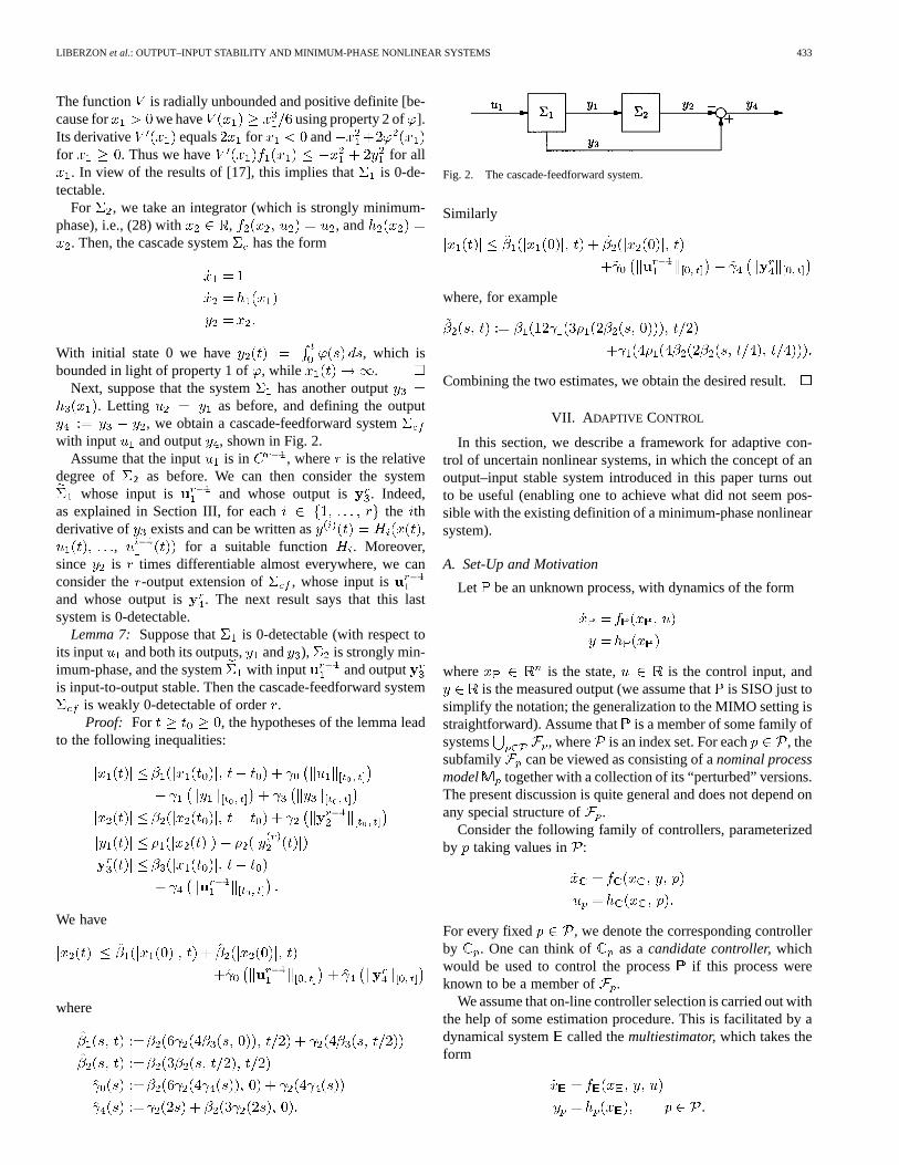
Next, suppose that the system has another output. Letting as before, and defining the output

, we obtain a cascade-feedforward systemwith input and output , shown in Fig. 2.

Assume that the input is in , where is the relativedegree of as before. We can then consider the system

whose input is and whose output is . Indeed,as explained in Section III, for each the thderivative of exists and can be written as ,

, for a suitable function . Moreover,since is times differentiable almost everywhere, we canconsider the -output extension of , whose input isand whose output is . The next result says that this lastsystem is 0-detectable.

Lemma 7: Suppose that is 0-detectable (with respect toits input and both its outputs, and ), is strongly min-imum-phase, and the system with input and outputis input-to-output stable. Then the cascade-feedforward system

is weakly 0-detectable of order.Proof: For , the hypotheses of the lemma lead

to the following inequalities:

We have

where

Fig. 2. The cascade-feedforward system.

Similarly

where, for example

Combining the two estimates, we obtain the desired result.

VII. A DAPTIVE CONTROL

In this section, we describe a framework for adaptive con-trol of uncertain nonlinear systems, in which the concept of anoutput–input stable system introduced in this paper turns outto be useful (enabling one to achieve what did not seem pos-sible with the existing definition of a minimum-phase nonlinearsystem).

A. Set-Up and Motivation

Let be an unknown process, with dynamics of the form

where is the state, is the control input, andis the measured output (we assume thatis SISO just to

simplify the notation; the generalization to the MIMO setting isstraightforward). Assume that is a member of some family ofsystems , where is an index set. For each , thesubfamily can be viewed as consisting of anominal processmodel together with a collection of its “perturbed” versions.The present discussion is quite general and does not depend onany special structure of .

Consider the following family of controllers, parameterizedby taking values in :

For every fixed , we denote the corresponding controllerby . One can think of as acandidate controller,whichwould be used to control the processif this process wereknown to be a member of .

We assume that on-line controller selection is carried out withthe help of some estimation procedure. This is facilitated by adynamical system called themultiestimator,which takes theform


The signals are used to define theestimation errors

One usually designs the multiestimator in such a way thatconverges to zero in the case when the unknown process coin-cides with the th nominal process model and there are nodisturbances or noise.

Most of the standard adaptive algorithms are based on varyingthe index of the candidate controller in the feedback loop ac-cording to a tuning/switching law , in such a waythat the corresponding estimation erroris maintained smallin some sense. The underlying principle behind such a strategyis known ascertainty equivalence.Intuitively, the motivationhere is that the nominal process model with the smallest esti-mation error “best” approximates the actual process, and thus,the candidate controller associated with that model can be ex-pected to do the best job of controlling the process. To justifythis paradigm, one must be able to ensure that the smallnessof the estimation error implies the smallness of the state of theclosed-loop system. Thus we see that a crucial desired propertyof this system is 0-detectability through the estimation error.

To make this discussion more precise, take an arbitrary fixed. The closed-loop system, which results when theth

candidate controller is placed in the feedback loop with theprocess and the multiestimator , is described by the equa-tions

(30)

We will take the output of this system to be the estimation error. A glance at Fig. 3 might be helpful

at this point. The above remarks suggest that it is desirable todesign the system (30) so as to make it 0-detectable with respectto .

Consider the following system, which we call theinjectedsystemand denote by :

We view it as a system with input , state , and out-puts and . It realizes the interconnection of theth candidate controller with the multi-estimator . This is

the system enclosed in the dashed box in Fig. 3. Basically, thechoice of the candidate controllers is governed by the resultingproperties of this system. This makes sense becauseis imple-mented by the control designer; the validity of such an approachwill become clear in view of the results that are discussed next.

It was shown in [5] that if the injected system is ISSwith respect to and the process is 0-detectable, then theclosed-loop system (30) is 0-detectable with respect to.This provided a natural nonlinear extension of the CertaintyEquivalence Stabilization Theorem proved for linear systemsin [11]. Another relevant result from [11] is the so-calledCertainty EquivalenceOutput Stabilization Theorem, whichwe mentioned in Section I. It suggests that the desired 0-de-tectability of the system (30) through should be preserved ifone weakens the assumptions on the injected systembyonly requiring input-to-output stability from to instead

Fig. 3. The closed-loop system (30).

of input-to-state stability,3 but demands that the process beoutput–input stable rather than 0-detectable. In what follows,we demonstrate that a result along these lines indeed holds fornonlinear systems.

B. Main Result and Discussion

Assume that has a known relative degree. Let us redefinethe input and the output of the system to be and ,respectively. We denote the resulting system by ; its outputmap is obtained as explained in the previous sections. We nowmake the following assumptions:

1) the process is strongly minimum-phase;2) the system is input-to-output stable;3) the controller is 0-detectable;4) the multiestimator is 0-detectable.

The result given below states that the-output extension of theclosed-loop system (30) is 0-detectable with respect to its output

(the derivatives of exist since we only consider smoothsystems; also note that there are no inputs). This result is a directconsequence of Lemma 7: one needs to apply that lemma with

(which is easily seen to be a 0-detectable system)and .

Theorem 3: Under assumptions 1–4, the closed-loop system(30) is weakly 0-detectable of order.

The same techniques would apply readily if the processis output–input stable but not necessarily strongly minimum-phase. In particular, if satisfies the hypotheses of part 1 ofTheorem 1 with , we would conclude weak 0-detectabilityof order for the closed-loop system. However, for thisis a weaker statement than that provided by Theorem 3.

Theorem 3 gives weak 0-detectability, i.e., 0-detectabilitythrough the output and derivatives of the output up to order. For linear systems the distinction between 0-detectability

and weak 0-detectability disappears; this is most easily seenfrom the well-known Kalman observability decomposition.It is possible to employ similar ideas to single out a classof nonlinear systems for which weak 0-detectability implies0-detectability. Namely, suppose that in some coordinates thesystem under consideration takes the form

(31)

3A careful examination of the classical model reference adaptive control al-gorithm for linear systems reveals that the control law only output stabilizes theestimated model.


with and , where the subsystem, is 0-detectable. This can be compared with

the observability decompositions for nonlinear systems (see,e.g., [2] or [12, Ch. 3]); we replace observability with 0-de-tectability (neither property is weaker than the other) and re-quire the decomposition to be global. Now, suppose that (31)is weakly 0-detectable of order, where is some positive in-teger. Since , where is a suitable classfunction (cf. proof of Proposition 1), we must have

for some and .Combining this with 0-detectability of the subsystem andusing the same arguments as the ones employed in Section VIfor dealing with cascade systems, we see that (31) is indeed0-detectable (through the original output).

Therefore, if the closed-loop system (30) with outputad-mits a decomposition of the kind described above, then underthe assumptions of Theorem 3 this system is 0-detectable. In thiscase we arrive at a strengthened version of Theorem 3 which ismore suitable for adaptive control applications. Of course, theexistence of such a decomposition may be difficult to verify inpractice. We also point out that the need to maintain smallnessof the estimation error together with its first derivative is not un-common in adaptive control (see, e.g., [9, Chs. 5 and 6]). Preciseimplications of Theorem 3 for adaptive control of nonlinear sys-tems remain to be investigated.

VIII. O UTPUT–INPUT STABILITY OF INPUT–OUTPUT

OPERATORS

It is possible to define the output–input stability propertyfor input–output operators, without relying on state-spacerepresentations. It then turns out that output–input stabilityof a system implies output–input stability of the associatedinput–output operator, and under suitable reachability andobservability assumptions, a converse result also holds. Herewe make some brief preliminary remarks on this; details willbe pursued elsewhere.

Given a pair of integers and and a subinterval of, we denote by the space of all times contin-

uously differentiable functions . By aninput–outputoperator, we mean a causal mapping

(32)

where , , , and are positive integers. “Causal” means thatif , then does not depend on the values ,

. Let us call an input–output operator (32)output–inputstableif there exist a positive integer , a classfunction , and a class function such that for everyinput and every pair of times inthe domain of the corresponding output we have

(33)

We now take to be the input–output operator that describesthe input–output mapping of the system (1), with .We want to understand the relationship between output–inputstability of the system and of the operator. What follows closelyparallels the developments of [15, Prop. 3.2 and 7.1].

Suppose that the system (1) is output–input stable. As the do-main of , we can take , so that the corre-sponding outputs are in . Here is the positive integer thatappears in (2). We could also work with in-stead, if is the relative degree of (1). It is not difficult to provethat is then output–input stable.

The converse is more interesting. Suppose that isoutput–input stable. We assume that the domain ofis , where is the positive integerthat appears in (33). As before, we could work with

instead, if is the relative degree of(1). We impose the following two assumptions on the system(1).

Assumption 1 (Strong Finite-Time Observability WithOutput Derivatives):There exist a number and twoclass functions and such that for every , everyinput , and every ,where is the maximal interval of existence of thecorresponding solution of (1), we have

(34)

Assumption 2 (Reachability With Bounded Over-shoot): There exists a class function such thatfor each it is possible to find a time and a controlinput which steers (1) from state 0at time to state at time in such a way that thecorresponding output satisfies

(35)

Under appropriate conditions, this second property can be de-rived from the strong reachability property considered in [15].Under these assumptions, it is possible to prove that for every

and every input the solution of(1) satisfies the inequalities

(36)

(37)

for all , where and . This isvery similar to output–input stability, except for the “noncausal”

in (37).

IX. CONCLUSION

We introduced a new concept of output–input stability, whichcan be viewed as an ISS-like variant of the minimum-phaseproperty for general smooth nonlinear control systems and re-duces to the classical minimum-phase property for linear sys-tems. We provided characterizations of output–input stability interms of suitably defined notions of detectability and relative de-gree, the latter of which was proposed here and is of independentinterest. Implications of the output–input stability property forfeedback stabilization, analysis of cascade systems, and adap-tive control were investigated. Other applications are likely to befound in various areas of nonlinear control theory in which theconcept of a minimum-phase nonlinear system has been useful.

ACKNOWLEDGMENT

Helpful discussions with J. Hespanha, A. Ilchmann, B. In-galls, A. Isidori, and M. Krichman are gratefully acknowledged.


REFERENCES

[1] D. Angeli, E. Sontag, and Y. Wang, “A note on input-to-state stabilitywith input derivatives,” inProc. 5th IFAC Symp. Nonlinear Control Syst.,2001, pp. 720–725.

[2] V. N. Brandin and G. N. Razorenov, “Decomposability conditionson nonlinear dynamic systems,”Automat. Rem. Control, vol. 37, pp.1789–1795, 1976.

[3] C. I. Byrnes and A. Isidori, “Local stabilization of minimum phase non-linear systems,”Syst. Control Lett., vol. 11, pp. 9–17, 1988.

[4] , “Asymptotic stabilization of minimum phase nonlinear systems,”IEEE Trans. Automat. Contr., vol. 36, pp. 1122–1137, Oct. 1991.

[5] J. P. Hespanha and A. S. Morse, “Certainty equivalence implies de-tectability,” Syst. Control Lett., vol. 36, pp. 1–13, 1999.

[6] A. Isidori, Nonlinear Control Systems, 3rd ed. Berlin, Germany:Springer-Verlag, 1995.

[7] M. Krichman and E. D. Sontag, “A version of a converse Lyapunovtheorem for input–output to state stability,” inProc. 37th IEEE Conf.Decision Control, 1998, pp. 4121–4126.

[8] M. Krichman, E. D. Sontag, and Y. Wang, “Input–output-to-state sta-bility,” SIAM J. Control Optim., vol. 39, pp. 1874–1928, 2001.

[9] M. Krstic, I. Kanellakopoulos, and P. V. Kokotovic´,Nonlinear and Adap-tive Control Design. New York: Wiley, 1995.

[10] A. S. Morse, “Structural invariants of linear multivariable systems,”SIAM J. Control Optim., vol. 11, pp. 446–465, 1973.

[11] , “Toward a unified theory of parameter adaptive control, PartII: Certainty equivalence and implicit tuning,”IEEE Trans. Automat.Contr., vol. 37, pp. 15–29, Jan. 1992.

[12] H. Nijmeijer and A. J. van der Schaft,Nonlinear Dynamical ControlSystems. New York: Springer-Verlag, 1990.

[13] L. Praly and Z. P. Jiang, “Stabilization by output feedback for systemswith ISS inverse dynamics,”Syst. Control Lett., vol. 21, pp. 19–33, 1993.

[14] L. M. Silverman and H. J. Payne, “Input–output structure of linearsystems with application to the decoupling problem,”SIAM J. ControlOptim., vol. 9, pp. 199–233, 1971.

[15] E. D. Sontag, “Smooth stabilization implies coprime factorization,”IEEE Trans. Automat. Contr., vol. 34, pp. 435–443, Apr. 1989.

[16] , Mathematical Control Theory: Deterministic Finite DimensionalSystems, 2nd ed. New York: Springer-Verlag, 1998.

[17] E. D. Sontag and Y. Wang, “Output-to-state stability and detectability ofnonlinear systems,”Syst. Control Lett., vol. 29, pp. 279–290, 1997.

[18] , “Notions of input to output stability,”Syst. Control Lett., vol. 38,pp. 235–248, 1999.

[19] W. M. Wonham,Linear Multivariable Control: A Geometric Approach,3rd ed. New York: Springer-Verlag, 1985.

Daniel Liberzon (M’98) was born in Kishinev,former Soviet Union, in 1973. He was a studentin the Department of Mechanics and Mathematicsat Moscow State University, Russia, from 1989 to1993, and received the Ph.D. degree in mathematicsfrom Brandeis University, Waltham, MA, in 1998(under the supervision of R. W. Brockett of HarvardUniversity, Cambridge, MA).

He was a Postdoctoral Associate in the Depart-ment of Electrical Engineering at Yale University,New Haven, CT, from 1998 to 2000. Since 2000, he

has been with the University of Illinois at Urbana-Champaign as an AssistantProfessor in the Electrical and Computer Engineering Department, and anAssistant Research Professor in the Coordinated Science Laboratory. Hisresearch interests include nonlinear control theory, analysis and synthesisof hybrid systems, switching control methods for systems with imprecisemeasurements and modeling uncertainties, and stochastic differential equationsand control.

Dr. Liberzon has served as an Associate Editor on the IEEE Control SystemsSociety Conference Editorial Board. Further details of his work can be found athttp://black.csl.uiuc.edu/~liberzon

A. Stephen Morse(S’62–M’67–SM’78–F’84) wasborn in Mt. Vernon, NY, in 1939. He received theB.S.E.E. degree from Cornell University, Ithaca, NY,in 1962, the M.S. degree from the University of Ari-zona, Tucson, in 1964, and the Ph.D. degree fromPurdue University, West Lafayette, IN, all in elec-trical engineering, in 1962, 1964, and 1967, respec-tively.

From 1967 to 1970, he was associated with the Of-fice of Control Theory and Application, NASA Elec-tronics Research Center, Cambridge, MA. Since July

1970, he has been with Yale University, New Haven, CT, where he is currentlya Professor of electrical engineering. His main interest is in system theory, andhe has done research in network synthesis, optimal control, multivariable con-trol, adaptive control, urban transportation, and hybrid and nonlinear systems.He has served as an Associate Editor of theEuropean Journal of Controlandthe International Journal of Adaptive Control and Signal Processing, and as aDirector of the American Automatic Control Council representing the Societyfor Industrial and Applied Mathematics.

Dr. Morse is a member of SIAM, Sigma Xi, and Eta Kappa Nu. He has servedas an Associate Editor of the IEEE TRANSACTIONS ONAUTOMATIC CONTROL.He was the recipient of the 1999 IEEE Control Systems Award. He is a Distin-guished Lecturer of the IEEE Control Systems Society, and a co-recipient of theSociety’s George S. Axelby Outstanding Paper Award. He has twice receivedthe American Automatic Control Council’s Best Paper Prize. Further details ofhis work can be found at http://entity.eng.yale.edu/controls

Eduardo D. Sontag (SM’87–F’93) received the Licenciado degree (mathe-matics) from the University of Buenos Aires, Argentina, and the Ph.D. degree(mathematics) under R. E. Kalman, at the Center for Mathematical SystemsTheory, University of Florida, Gainesville, in 1972 and 1976, respectively.

Since 1977, he has been with the Department of Mathematics, Rutgers Uni-versity, New Brunswick, NJ, where he is currently Professor II of Mathematics,as well as a Member of the Graduate Faculties of the Department of ComputerScience and of the Department of Electrical and Computer Engineering. Heis also the Director of the Rutgers Center for Systems and Control. His majorcurrent research interests are in several areas of control theory and biologicallyinspired mathematics. He has authored nearly 300 journal and conferencepapers and book chapters, as well as the booksTopics in Artificial Intelligence(in Spanish, Buenos Aires, Argntina: Prolam, 1972),Polynomial ResponseMaps (Berlin, Germany: Springer-Verlag, 1979), andMathematical ControlTheory: Deterministic Finite Dimensional Systems(2nd ed., New York:Springer-Verlag, 1998). His industrial experience includes consulting for BellLaboratories, Holmdel, NJ, and Siemens, New York, NY. He is an AssociateEditor for various journals, includingSMAI-COCOV, Dynamics and Control,Journal of Computer and Systems Sciences, Neurocomputing, and NeuralComputing Surveys(Board of Advisors). He is a former Associate Editor ofControl-Theory and Advanced TechnologyandSystems and Control Letters. Inaddition, he is a co-founder and co-Managing Editor of the Springer journalMathematics of Control, Signals, and Systems(MCSS).

Dr. Sontag was awarded the Reid Prize in Mathematics by SIAM, the Societyfor Industrial and Applied Mathematics, in July 2001. He is also a former As-sociate Editor of the IEEE TRANSACTIONS ONAUTOMATIC CONTROL and theIEEE TRANSACTIONS ONNEURAL NETWORKS. Further details of his work canbe found at http://www.math.rutgers.edu/~sontag

Documents

Output-input stability and minimum-phase nonlinear … IEEE TRANSACTIONS ON AUTOMATIC CONTROL, VOL. 47, NO. 3, MARCH 2002 Output–Input Stability and Minimum-Phase Nonlinear Systems