Embed Size (px)
Citation preview

Indus Journal of Management & Social Sciences, 3(1):39-51 (Spring 2009) http://indus.edu.pk/journal.php
Output Maximization of an Agency By P. Moolio, J. N. Islam, and H.K. Mohajan
39
Output Maximization of an Agency
Pahlaj Moolio *, Jamal Nazrul Islam **, and Haradhan Kumar Mohajan***
ABSTRACT
Considering Cobb-Douglas function in three variables as an explicit form of production function, in this paper an attempt has been made to maximize an output subject to a budget constraint, using Lagrange multipliers technique, as well as necessary and sufficient conditions for optimal value have been applied. We gave interpretation of Lagrange multiplier in this specific illustration, showing its positive value, and examined the behavior of the agency. JEL. Classification: C31; D24; I38; L21; L25; M11 Key words: Lagrange Multipliers; Economic Problems; Maximizing Output Function; Budget Constraints; Explicit Examples. 1. INTRODUCTION The method of Lagrange multipliers is a very useful and powerful technique in multivariable calculus and has been used to facilitate the determination of necessary conditions; normally, this method was considered as device for transferring a constrained problem to a higher dimensional unconstrained problem (Islam 1997, Pahlaj and Islam 2008). Using this technique, Baxley and Moorhouse (1984) analyzed an example of utility maximization, and provided a formulation for nontrivial constrained optimization problem with special reference to application to economics. They considered implicit functions with assumed characteristic qualitative features and provided illustration of an example, generating meaningful economic behaviour. This approach and formulation may enable one to view optimization problems in economics from a somewhat wider
The material presented by the authors does not necessarily represent the viewpoint of editors and the management of Indus Institute of Higher Education (IIHE) as well as the authors’ institute. * Ph.D. Fellow, Research Centre for Mathematical and Physical Sciences, University of Chittagong, Chittagong, Bangladesh; and Professor and Academic Advisor, Pannasastra University of Cambodia, Phnom Penh, Cambodia. Corresponding Author: Pahlaj Moolio. E-mail: [email protected] ** Emeritus Professor, Research Centre for Mathematical and Physical Sciences, University of Chittagong, Chittagong, Bangladesh. Phone: +880-31-616780. *** Lecturer, Premier University, Chittagong, Bangladesh , E mail: [email protected] Acknowledgements: Authors would like to thank the editors and anonymous referees for their comments and insight in improving the draft copy of this article. Authors furthur would like to declare that this manuscript is original and has not previously been published, and that it is not currently on offer to another publisher; and also transfer copy rights to the publisher of this journal. Recieved: 03-12- 2008; Revised: 20-01-2008; Accepted: 15-04-2009; Published: 20-04-2009

Indus Journal of Management & Social Sciences, 3(1):39-51 (Spring 2009) http://indus.edu.pk/journal.php
Output Maximization of an Agency By P. Moolio, J. N. Islam, and H.K. Mohajan
40
perspective. Using this technique, Pahlaj and Islam (2008) considered a problem of cost minimization in three variables subject to output function as a constraint, studying the behaviour of the firm, and hence extended the work of Pahlaj (2002). Detailed discussion of the Lagrange multipliers method and its use in economics is given in Islam (2008). In this paper, we consider theoretically a variation of the problem considered by Pahlaj and Islam (2008), assuming that a government agency is allocated an annual budget B and required to maximize and make available some sort of services to the community. If the agency uses factors
and , , LK R in the same sense as used by Pahlaj and Islam (2008) to produce and provide services to the community, then its objective is to maximize the output function subject to a budget constraint. This problem is thus the dual to the cost minimization of a competitive firm, considered by Pahlaj and Islam (2008). In section 2, we deal with formulating mathematical model for the problem, considering Cobb-Douglas production function in three variables (factors: capital, labour, and other inputs). Considering an explicit form of production function, we apply necessary conditions to this output maximization problem, and find stationary point as well as optimal value of the production function in section 3. In section 4, we give a reasonable interpretation of the Lagrange multiplier in the context of this particular illustration. Sufficient conditions are applied in section 5. In section 6, we analyze the comparative static results (Chiang 1984) and examine the behaviour of the agency; that is, how a change in the input costs will affect the situation, or if the budget for the services undergoes some changes. In final section 7, we provide conclusion and recommendations. 2. THE MATHEMATICAL MODEL We consider that, for the fixed annual budget, a government agency is charged to produce and provide to the community with the quantity Q units of the services during a specified time, say for instance, in a year, with the use of K quantity of capital, quantity of labour, and L R quantity of other inputs into its service oriented production process. These other inputs (e.g., land and other raw materials) are combined to produce the production (Humphery 1997; Pahlaj and Islam 2008). If the agency uses factors and , , LK R to produce and provide quantity Q units of the services (Baxley and Moorhouse 1984; Pahlaj and Islam 2008) to the community, then its objective is to maximize the output function:
( RLKgQ , , = ) , (1) subject to the budget constraint:
RwLrKB ρ++= , (2) where r is the rate of interest or services per unit of capital is the wage rate per unit of labour , and
wK ,L ρ is the cost per unit of other inputs R , while g is a suitable production function.
The government agency takes these and all other factor prices as given. We assume that second order partial derivatives of the function g with respect to the independent variables (factors)
and , , LK R exist.

Indus Journal of Management & Social Sciences, 3(1):39-51 (Spring 2009) http://indus.edu.pk/journal.php
Output Maximization of an Agency By P. Moolio, J. N. Islam, and H.K. Mohajan
41
Ignoring the actual form of the function Q , we now formulate the maximization problem for the output function given by (1) in terms of single Lagrange multiplier λ , by defining the Lagrangian function Z as follows: ( ) ( ) ( )RwLrKBRLKQRLKZ ρλλ −−−+= , , , , , . (3)
This is a four dimensional unconstrained problem obtained from (1) and (2) by the use of Lagrange multiplier λ , as a device. Assuming that the government agency maximizes its output, the optimal quantities of **** and , , , λRLK λ and , , , RLK that necessarily satisfy the first order conditions; which can be obtained by partially differentiating the Lagrangian function (3) with respect to four variables RLK and , , ,λ and setting them equal to zero:
0=−−−= RwLrKBZ ρλ , (4a)
0=−= rQZ KK λ , (4b)
0=−= wQZ LL λ , (4c)
0=−= λρRR QZ , (4d) where
RgQ
LgQ
KgQZZ
RZZ
LZZ
KZZ RLKRLK ∂
∂=
∂∂
=∂∂
=∂∂
=∂∂
=∂∂
=∂∂
= , , and , , , ,λλ .
It may be noted that the partial derivative with respect to λ is just the same as the constraint - this is always the case, so we get again RwLrKB ρ++= , while from (4b-d), the Lagrange multiplier is obtained as follows:
ρλ RLK Q
wQ
rQ
=== . (5)
Considering the infinitesimal changes in , respectively, and the corresponding changes , we get:
dRdLdK , , RLK , ,dBdQ and
dRQdLQdKQdQ RLK ++= , (6) dRwdLrdKdB ρ++= . (7)
With the use of (4b-d) or (5), we obtain the following equation:
λρ
=++++
=dRwdLrdK
dRQdLQdKQdBdQ RLK . (8)
Thus, the Lagrange multiplier gives the change in total output consequent to change in the inputs. If, for example, one of the inputs, say is held constant, means ,K 0=dK , then (8) represents the
partial derivative: KB
Q⎟⎠⎞
⎜⎝⎛∂∂
(with 0=dK ), and so.

Indus Journal of Management & Social Sciences, 3(1):39-51 (Spring 2009) http://indus.edu.pk/journal.php
Output Maximization of an Agency By P. Moolio, J. N. Islam, and H.K. Mohajan
42
3. AN EXPLICIT EXAMPLE We now consider an explicit form of the output function in (1), and provide a detailed discussion and intrinsic understanding of the problem at hand.
g
Let the function given by g( ) γβα RLAKRLKgQ == , , , (9)
where is assumed to be unchanged technology; and the exponents A γβα and , , are constants that constitute the output elasticities with respect to capital, labour, and other inputs (Humphery 1997, and Pahlaj and Islam 2008), respectively. Using (2) and (9), (3) takes the following form: ( ) ( )RwLrKBRLAKRLKZ ρλλ γβα −−−+= , , , . (3a)
Therefore, (4a-d) become: 0=−−−= RwLrKBZ ρλ , (10a)
01 =−= − λα γβα rRLAKZ K , (10b)
01 =−= − λβ γβα wRLAKZ L , (10c)
01 =−= − ρλγ γβα RLAKZ R . (10d) Using the method of successful elimination and substitution, we solve above set of equations and obtain the optimum values of λ and , , , RLK :
( )γβαα
++==
rBKK * . (11a)
( )γβαβ
++==
wBLL * . (11b)
( )γβαργ
++==
BRR * (11c)
( )
( )( ) ⎟⎟⎠
⎞⎜⎜⎝
⎛
++⎟⎟⎠
⎞⎜⎜⎝
⎛== −++
−++
1
1*
γβα
γβα
γβα
γβα
γβαργβαλλ B
wrA . (11d)
Thus, the stationary point is as below:
( ) ( ) ( ) ( )⎟⎟⎠⎞
⎜⎜⎝
⎛++++++
=γβαρ
γγβα
βγβα
α Bw
Br
BRLK ,,,, *** . (12)
Moreover, substituting the values of from (11a-c) into (9), we get the optimal value of the production function in terms of
*** , , RLKγβαρ , , and , , , , , BAwr as follows:

Indus Journal of Management & Social Sciences, 3(1):39-51 (Spring 2009) http://indus.edu.pk/journal.php
Output Maximization of an Agency By P. Moolio, J. N. Islam, and H.K. Mohajan
43
( )
( )( ) ⎟⎟⎠
⎞⎜⎜⎝
⎛
++= ++
++
γβαγβα
γβαγβα
γβαργβα
wrBAQ* . (13)
4. INTERPRETATION OF LAGRANGE MULTIPLIER Before we discuss sufficient conditions and analyze comparative static results, we provide an interpretation of Lagrange multiplier. To some extent, this might seem a bit silly to talk about the meaning of an artificial variable added for computational convenience, but bear with me there is a reasonable interpretation of this variable. With the aid of chain rule, from (13) we get:
BRQ
BLQ
BKQ
BQ
RLK ∂∂
+∂∂
+∂∂
=∂∂ *
(14)
From (9), we get: , , . γβαα RLAKQK1−= γβαβ RLAKQL
1−= 1−= γβαγ RLAKQR
And from (10b-d), we get: , , . γβααλ RLAKr 1−= γβαβλ RLAKw 1−= 1−= γβαγρλ RLAKTherefore, we write (14) as follows:
⎥⎦⎤
⎢⎣⎡
∂∂
+∂∂
+∂∂
=∂∂
BR
BLw
BKr
BQ ρλ*
*
. (15)
From (10a), we have: RwLrKB ρ++= . Differentiating above equation, keeping constants, we get: RLK and , ,
BR
BLw
BKr
∂∂
+∂∂
+∂∂
= ρ1 ,
which allows us to rewrite (15) as:
**
λ=∂∂
BQ
. (16)
Therefore, (16) verifies (8). Thus, the Lagrange multiplier may be interpreted as the marginal output, that is, the change in total output incurred from an additional unit of budget
*λB . In other
words, in this particular illustration, if the agency wants to increase (decrease) 1 unit of its output, it would cause the total budget to increase (decrease) by approximately units. This is a reasonable interpretation.
*λ
5. SUFFICIENT CONDITIONS Now, in order to be sure that the optimal solution obtained in (12) is maximum; we check it against the sufficient conditions, which imply that for a solution of (10a-d) to be a relative maximum, all the bordered principal minors of the following bordered Hessian,
**** and , , , λRLK

Indus Journal of Management & Social Sciences, 3(1):39-51 (Spring 2009) http://indus.edu.pk/journal.php
Output Maximization of an Agency By P. Moolio, J. N. Islam, and H.K. Mohajan
44
RRRLRKR
LRLLLKL
KRKLKKK
RLK
ZZZBZZZBZZZB
BBB
H
−−−
−−−
=
0
,
should take the alternate sign, namely, the sign of 1+mH being that of ( ) 11 +− m , where m is the
number of constraints. In our case 1=m , therefore, in this specific case, if
00
2 >−−
−−=
LLLKL
KLKKK
LK
ZZBZZB
BBH , (17a)
and 0
0
3 <
−−−
−−−
==
RRRLRKR
LRLLLKL
KRKLKKK
RLK
ZZZBZZZBZZZB
BBB
HH , (17b)
with all the derivatives evaluated at the critical values of , then the stationary value of obtained in (13) will assuredly be the maximum. We check this condition, through
expanding the determinant (17a) first, noticing that the second partial derivative of :
**** and , , , λRLKQ
LKKL ZZ =
KKLLKLLKLLKK ZBBZBBZBBH −+−= 22 . (18)
From (2) and (10b-d), we get: rBK = ; ; wBL = ρ=RB . (19a)
( ) γβααα RLAKZ KK21 −−= ; ; ( ) γβαββ RLAKZ LL
21 −−=( ) 21 −−= γβαγγ RLAKZ RR . (19b)
γβααβ RLAKZZ LKKL11 −−== ; ; 11 −−== γβααγ RLAKZZ RKKR
11 −−== γβαβγ RLAKZZ RLLR . (19c) Substitution of the values of from (19a-c) into (18) yields: KLLLKKLK ZZZBB , , , ,
( )2222211222222 2 −−−−−− +−++−= KwKwLKrwLrLrRLAKH αααβββγβα .

Indus Journal of Management & Social Sciences, 3(1):39-51 (Spring 2009) http://indus.edu.pk/journal.php
Output Maximization of an Agency By P. Moolio, J. N. Islam, and H.K. Mohajan
45
Substitution of the critical values of from (11a-c) into above equation, and after straightforward but tedious calculation yields:
*** , , RLK
. where
,2
222
2
γβαψ
ψψρ
γβααβ
βαψγβα
ψγβα
++=
⎟⎟⎠
⎞⎜⎜⎝
⎛⎟⎟⎠
⎞⎜⎜⎝
⎛⎟⎟⎠
⎞⎜⎜⎝
⎛ +=
Bwr
wrBAH
(20a)
Similarly, from (17b), we expand the determinant, noticing that the second partial derivative of
RLLRRKKRLKKL ZZZZZZ === and , , :
.2 222
22
KLKLRRLLKKRRKLKRRLKRKRLL
LRKKRLRRKKLLLLKRRKLRKRLK
LRKLRKRRKLLKLRLRKKRRLLKK
ZZBBZZBBZZBBZZBBZZBBZZBBZZBBZZBB
ZZBBZZBBZZBBZZBBH
+−−++−+−
−++−=
Substituting the values of from (19a-c) into above equation, and after straightforward but tedious calculation, we get:
LRKRKLRRLLKKRLK ZZZZZZBBB , , , , , , , ,
⎪⎪
⎭
⎪⎪
⎬
⎫
⎪⎪
⎩
⎪⎪
⎨
⎧
−+
+−−
++−
−−+
=
−−−−
−−−−−−−
−−−−−−−
−−−−−−−−−
222222
2222112222
2222222121
21122222222222
2222
22
2
LKLKLKRLKwRKw
RKwRKwRLKrRLKrwRLrRLrRLr
RLKAH
αβραβρ
βαρραβγαγ
αγγαραβγ
αβγβγβγγβ
γβα .
Similarly, by substituting the critical values of from (11a-c) into above equation, and after straightforward but tedious calculation, we get:
*** , , RLK
. where
,4
5222
2222
22222
γβαψαβγ
ψρψρ
γβαψγβα
ψγβα
++=
⎟⎟⎠
⎞⎜⎜⎝
⎛⎟⎟⎠
⎞⎜⎜⎝
⎛−=
Bwr
wrBAH
(20b)
Since ,0 ,0 ,0 ,0 >>>> γβαA and ρ, , wr are the costs of inputs and hence are positive,
while B is budget that will never be negative, therefore, from (20a) 02 >H and from (20b)
0<H , as required by (17a) and (17b), respectively. Equations (20a) and (20b) are sufficient
conditions satisfied to state that the stationary point obtained in (12) is a relative maximum point. Thus, the value of the output function obtained in (13) is indeed a relative maximum value.

Indus Journal of Management & Social Sciences, 3(1):39-51 (Spring 2009) http://indus.edu.pk/journal.php
Output Maximization of an Agency By P. Moolio, J. N. Islam, and H.K. Mohajan
46
6. COMPARATIVE STATIC ANALYSIS Now, since sufficient conditions are satisfied, we drive further results of economic interest. Mathematically, we solve the four equations in (10a-d) for λ and , , , RLK in terms of
Bwr and , , , ρ , and compute sixteen partial derivatives: ,,LrK∂∂ ,,L
rL∂∂ ,,L
rR∂∂ ,,L
r∂∂λ
etc.
hese partial derivatives are referred to as the comparative static of the model. The model’s T
usefulness is to determine how accurately it predicts the adjustments in the agency’s input behaviour, that is, how the agency will react to the changes in the costs of capital, labour, and other inputs. Since we have assumed that the left side of each equation in (10) is continuously differentiable and that the solution exists, then by the Implicit Function Theorem λ and , , , RLK will each be continuously differentiable function of Bwr and , , , ρ , if the Jacobian
⎤⎡ −−− RLK BBB0 matrix
⎥⎥⎥⎥
⎦⎢⎢⎢⎢
⎣−−−
=
RRRLRKR
LRLLLKL
KRKLKKK
ZZZBZZZBZZZB
J , (21)
is non-singular at the optimum point ( )**** , , , λRLK . As the sufficient conditions are met, so the
t the optimum, thdeterminant of (21) does not vanish a at is, HJ = ; consequently we apply the
Implicit Function Theorem. Let F be the vector-valu ion defined for the point ed funct( ) 8**** , , , , , , , RBwrRLK ∈ρλ , d taking the values in 4an R , whose components are given by
-d). By the Implicit Functio heorem, the equation the left side of the equations in (10a n T
( ) 0 , , , , , , , **** =BwrRLKF ρλ , (22)
ay be solved in the form of
. (23)
oreover, the Jacobian matrix fo s given by
m
( )BwrG
RLK
, , ,
*
*
*
*
ρ
λ
=
⎥⎥⎥⎥⎥
⎦
⎤
⎢⎢⎢⎢⎢
⎣
⎡
M r G i

Indus Journal of Management & Social Sciences, 3(1):39-51 (Spring 2009) http://indus.edu.pk/journal.php
Output Maximization of an Agency By P. Moolio, J. N. Islam, and H.K. Mohajan
47
⎥⎥⎥⎥⎥
⎦
⎤
⎢⎢⎢⎢⎢
⎣
⎡
−−
−−−−
−=
⎥⎥⎥⎥⎥⎥⎥⎥⎥⎥
⎦
⎤
⎢⎢⎢⎢⎢⎢⎢⎢⎢⎢
⎣
⎡
∂∂
∂∂
∂∂
∂∂
∂∂
∂∂
∂∂
∂∂
∂∂
∂∂
∂∂
∂∂
∂∂
∂∂
∂∂
∂∂
−
0000000001
*
*
*
***
1
****
****
****
****
λλ
λ
ρ
ρ
ρ
λρλλλ
RLK
J
BRR
wR
rR
BLL
wL
rL
BKK
wK
rK
Bwr
, (24)
where the row in the last matrix on the right is obtained by differentiating the ith left side in (10) with respect to
ith,r then , then w ρ , and then B . Let be the cofactor of the element in the
row and column of , and then inverting using the method of cofactor gives: ijC
ith jth J JTC
JJ 11 =− , where ( )ijCC = .
Thus, following the matrix multiplication rule, (24) can further be expressed in the following form:
⎥⎥⎥⎥⎥
⎦
⎤
⎢⎢⎢⎢⎢
⎣
⎡
−−−−−−−−−−−−−−−−−−−−−−−−
−=
⎥⎥⎥⎥⎥⎥⎥⎥⎥⎥
⎦
⎤
⎢⎢⎢⎢⎢⎢⎢⎢⎢⎢
⎣
⎡
∂∂
∂∂
∂∂
∂∂
∂∂
∂∂
∂∂
∂∂
∂∂
∂∂
∂∂
∂∂
∂∂
∂∂
∂∂
∂∂
1444*
14*
34*
14*
24*
14*
1343*
13*
33*
13*
23*
13*
1242*
12*
32*
12*
22*
12*
1141*
11*
31*
11*
21*
11*
****
****
****
****
1
CCCRCCLCCKCCCRCCLCCKCCCRCCLCCKCCCRCCLCCK
J
BRR
wR
rR
BLL
wL
rL
BKK
wK
rK
Bwr
λλλλλλλλλλλλ
ρ
ρ
ρ
λρλλλ
. 25)
Now, we study the effects of changes in Bwr and , , , ρ on . Firstly, we find out the effect on capital
RLK and ,, K when it’s interest rate increases. From (25), we get:
[ ] .0
1 **
22*
12*
*
RRRLR
LRLLL
RL
RRRLR
LRLLL
KRKLK
ZZBZZB
BB
JZZBZZBZZB
JKCCK
JrK
−−
−−+
−−−
−=−−−=∂∂ λλ
Expansion of above determinants yields:
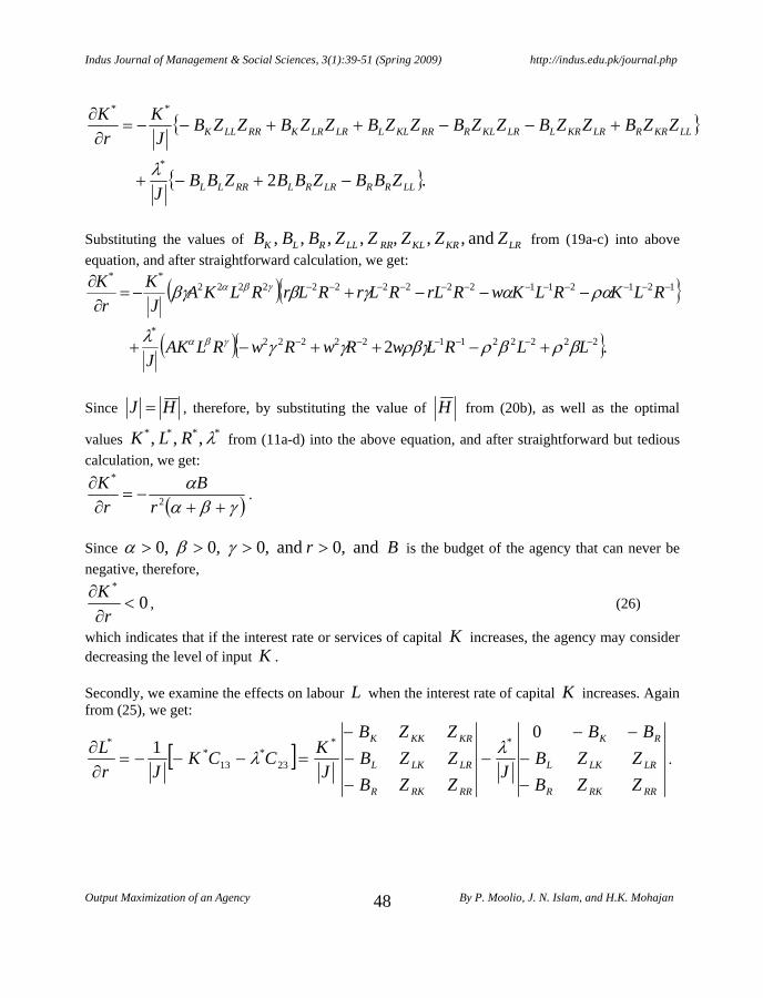
Indus Journal of Management & Social Sciences, 3(1):39-51 (Spring 2009) http://indus.edu.pk/journal.php
Output Maximization of an Agency By P. Moolio, J. N. Islam, and H.K. Mohajan
48
{ }
{ }.2 *
**
LLRRLRRLRRLL
LLKRRLRKRLLRKLRRRKLLLRLRKRRLLK
ZBBZBBZBBJ
ZZBZZBZZBZZBZZBZZBJ
Kr
K
−+−+
+−−++−−=∂∂
λ
Substituting the values of from (19a-c) into above equation, and after straightforward calculation, we get:
LRKRKLRRLLRLK ZZZZZBBB and , , , , , , ,
( ){ }
( ){ }.2 222221122222*
1212112222222222**
−−−−−−
−−−−−−−−−−−−
+−++−+
−−−+−=∂∂
LLRLwRwRwRLAKJ
RLKRLKwRrLRLrRLrRLKAJ
Kr
K
βρβρρβγγγλ
ρααγββγ
γβα
γβα
Since HJ = , therefore, by substituting the value of H from (20b), as well as the optimal
values from (11a-d) into the above equation, and after straightforward but tedious calculation, we get:
**** , , , λRLK
( )γβαα
++−=
∂∂
2
*
rB
rK
.
Since Br and ,0 and ,0 ,0 ,0 >>>> γβα is the budget of the agency that can never be negative, therefore,
0*
<∂∂
rK
, (26)
which indicates that if the interest rate or services of capital K increases, the agency may consider decreasing the level of input K . Secondly, we examine the effects on labour when the interest rate of capital L K increases. Again from (25), we get:
[ ]RRRKR
LRLKL
RK
RRRKR
LRLKL
KRKKK
ZZBZZB
BB
JZZBZZBZZB
JKCCK
JrL
−−
−−−
−−−
=−−−=∂∂
01 **
23*
13*
* λλ .

Indus Journal of Management & Social Sciences, 3(1):39-51 (Spring 2009) http://indus.edu.pk/journal.php
Output Maximization of an Agency By P. Moolio, J. N. Islam, and H.K. Mohajan
49
{ }
{ }. *
**
LKRRRKRLLRRKRRLK
LKKRRRKKRLLRKKRRRKKLLRRKKRRLKK
ZBBZBBZBBZBBJ
ZZBZZBZZBZZBZZBZZBJ
KrL
−++−−
+−−++−=∂∂
λ
By substituting the values of from (19a-c) into above equation, and after simplification, we get:
LRKRLKRRKKRLK ZZZZZBBB , , , , , , ,
( ){ }
( ){ }. 1121111222*
1122222222112222**
−−−−−−−−
−−−−−−−−−−−−
−+++−−
++−−=∂∂
LKRKwRLrRrwRrwRLAKJ
RLKRwKRKwRKwRLKrRLKAJ
KrL
αβρραγρβγγγλ
ρβγαβαγ
γβα
γβα
By substituting the optimal values of from (11a-d) into above equation, and after straightforward but tedious calculation, we get:
**** , , , λRLK
⎭⎬⎫
⎩⎨⎧
⎟⎟⎠
⎞⎜⎜⎝
⎛⎟⎟⎠
⎞⎜⎜⎝
⎛⎟⎟⎠
⎞⎜⎜⎝
⎛⎟⎟⎠
⎞⎜⎜⎝
⎛−⎟⎟
⎠
⎞⎜⎜⎝
⎛⎟⎟⎠
⎞⎜⎜⎝
⎛⎟⎟⎠
⎞⎜⎜⎝
⎛⎟⎟⎠
⎞⎜⎜⎝
⎛=
∂∂
3
32
2
2
222
222
3
32
2
2
222
2222* 11B
rwBwrB
rwBwrJ
ArL ψρ
ψργβα
γψρ
ψργβα
γ ψ
ψ
γβα
γβα
ψ
ψ
γβα
γβα
0*
=∂∂
rL
. (27)
This indicates that there will be no effect on the level of labour , if the interest rate of capital L K increases. This also indicates that in this case labour and capital are complement to each other. The above analysis relates to the effects of a change in interest rate of capital K ; our results are readily adaptable to the case of a change in wage rate of labour , as well as to a change in cost of other inputs
LR .
Next, we analyze the effect of a change in budget B . Suppose that the service-providing agency gets additional budget in order to increase it’s services; then naturally, we can expect that there will be an increase in its inputs of . We examine and verify this mathematically as follows. From (25), we get:
RLK and , ,
[ ]RRRLR
LRLLL
KRKLK
ZZBZZBZZB
JC
JBK
−−−
=−=∂∂ 11
12
*
.

Indus Journal of Management & Social Sciences, 3(1):39-51 (Spring 2009) http://indus.edu.pk/journal.php
Output Maximization of an Agency By P. Moolio, J. N. Islam, and H.K. Mohajan
50
{ }LLKRRRLKRLLRKLRRRKLLRLLRKRRLLK ZZBZZBZZBZZBZZBZZBJB
K+−−++−=
∂∂ 1*
. By substituting the values of from (19a-c) into above equation, and after simplification, we get:
LRKRLKRRLLRLK ZZZZZBBB , , , , , , ,
( ){ .1 1212112222222222*
−−−−−−−−−−−− −−−+=∂∂ RLKRLKwRrLRLrRLrRLKA
JBK ρααγββγ γβα }
Again, since HJ = , therefore, by putting the value of H from (20b), as well as the optimal
values of ,*K ,*L *R from (11a-c), and after straightforward calculation, we get:
( )γβαα
++=
∂∂
rBK *
.
Again, since 0 and ,0 ,0 ,0 >>>> rγβα , therefore,
0*
>∂∂
BK
. (28)
which verifies our assumption and common sense that when the budget size increases, the agency may consider increasing its level of inputs: capital, labour, and other inputs, in order to increase the
output services. Our results and discussion are true for 0*
>∂∂
BL
, 0*
>∂∂
BR
as well.
7. CONCLUSION AND RECOMMENDATIONS In this article, we have applied Lagrange multiplier method to an agency’s output maximization problem subject to budget constraint, using necessary and sufficient conditions for optimal values – in this particular case, maximization of the output of an agency. It is demonstrated that value of the Lagrange multiplier is positive, providing its reasonable interpretation; that is, if the agency is asked to increase (decrease) 1 unit of its output, it would cause total budget to increase (decrease) by approximately units. With the help of comparative static analysis and application of Implicit Function Theorem, we mathematically showed the behaviour of the agency, and suggest that if the cost of a particular input increases, the agency needs to consider decreasing the level of that particular input; at the same time, and there is no effect on level of other inputs. As well as, we demonstrated mathematically that when the budget increases the agency may consider increasing its level of inputs: capital, labour, and other inputs, in order to increase the output.
*λ
REFERENCES Baxley, J. V. and Moorhouse, J. C. 1984. Lagrange Multiplier Problems in Economics. The
American Mathematical Monthly, 91(7): 404-412 (Aug. – Sep).

Indus Journal of Management & Social Sciences, 3(1):39-51 (Spring 2009) http://indus.edu.pk/journal.php
Output Maximization of an Agency By P. Moolio, J. N. Islam, and H.K. Mohajan
51
Chiang, A.C. 1984. Fundamental Methods of Mathematical Economics. 3rd ed. Singapore: McGraw-Hill.
Humphery, T.M. 1997. Algebraic Production Functions and Their Uses before Cobb- Douglas. Federal Reserve Bank of Richmond Economic Quarterly, 83 (1) winter.
Islam, J. N. 1997. Aspects of Mathematical Economics and Social Choice Theory. Proceedings of
the Second Chittagong Conference on Mathematical Economics and its Relevance for Development. Ed. J. N. Islam, Chittagong: University of Chittagong, Bangladesh.
Islam, J. N. 2008. An Introduction to Mathematical Economics and Social Choice Theory, (book to
appear). Pahlaj M. 2002. Theory and Applications of Classical Optimization to Economic Problems. M. Phil.
Thesis. Chittagong: University of Chittagong, Bangladesh. Pahlaj M. and J.N. Islam. 2008. Cost Minimization of a Competitive Firm. Indus Journal of
Management and Social Sciences, 2(2):148-160 (Fall 2008).
*****