Embed Size (px)
Citation preview

by
Simone Borghesi, Chiara Franco, Giovanni Marin
Outward Foreign Direct Investments Patterns of Italian Firms in the EU ETS

SEEDS is an interuniversity research centre. It develops research and higher education projects in the fields of ecological and environmental economics, with a special focus on the role of policy and innovation. Main fields of action are environmental policy, economics of innovation, energy economics and policy, economic evaluation by stated preference techniques, waste management and policy, climate change and development.
The SEEDS Working Paper Series are indexed in RePEc and Google Scholar. Papers can be downloaded free of charge from the following websites: http://www.sustainability-seeds.org/. Enquiries:[email protected]
SEEDS Working Paper 01/2016 January 2016 by Simone Borghesi, Chiara Franco, Giovanni Marin
The opinions expressed in this working paper do not necessarily reflect the position of SEEDS as a whole.

1
Outward Foreign Direct Investments
Patterns of Italian Firms in the EU ETS
Simone Borghesi* Chiara Franco
† Giovanni Marin
‡
Abstract
We consider the role played by the EU Emission Trading System
(EU ETS) as a possible driver of outward Foreign Direct Investments
(FDI henceforth).
In particular, we aim at assessing whether EU ETS has any effect
on outward FDI patterns of Italian firms. Using a novel panel dataset
of about 59,000 firms covering the first two phases of the EU ETS and
the pre-EU ETS period, we are able to observe the patterns of FDI by
destination country of firms, distinguishing between those with plants
covered by the EU ETS and other firms. Results show that, on
average, firms in the EU ETS do not increase their presence in other
countries. However, EU ETS firms operating in sectors particularly
exposed to international competition increase their outward FDI
towards countries not covered by the EU ETS.
Keywords: EU ETS, FDI, carbon leakage
JEL: F23, L23, Q50
* University of Siena (Italy), [email protected].
† Catholic University of the Sacred Heart, Milano (Italy), [email protected].
‡ IRCrES-CNR, Research Institute for Sustainable Economic Growth, National Research Council of Italy,
Milano (Italy), [email protected].

2
1 Introduction
In the last few years the European Emission Trading Scheme (EU ETS) has attracted
much attention among scholars and policy-makers as it represents the central policy
instrument adopted by the EU to mitigate climate change. The capacity of the EU to
unilaterally develop the first transboundary system of emission trading has made the EU
ETS a prototype for several other ETSs that are rapidly spreading around the world
(Ellerman, 2010).
However, the lack of an internationally coordinated environmental policy has raised
increasing concerns about the potential competitiveness losses deriving from a stringent
unilateral environmental regulation like the EU ETS. In particular, it has been argued
that in the presence of global externalities such as the ones generated by CO2 emissions
unilateral environmental interventions may end up being not effective in environmental
terms while provoking socio-economic consequences in terms of job losses.
Some European production sectors are regarded as particularly vulnerable to the risk
of carbon leakage, i.e. the delocalisation of production (and corresponding carbon
emissions) of involved industries towards environmental policy-free geographical areas.
The issue of carbon leakage has been recognised by the Commission that exempted
from the auctioning of emission allowances those sectors more exposed to the risk of
leakage, at least for the second commitment period of the EU ETS (2013-2020).
Surprisingly enough, however, this debate on the risks of carbon leakage lacks
empirical evidence so far on whether the EU ETS can actually induce European firms to
change their location, moving their production towards countries that are not subject to
the EU ETS (to avoid the consequences of this regulation). Our paper aims at providing
empirical evidence on this relevant issue.
The relocation risks provoked by unilateral environmental regulation are the object
of a long-standing and extensive theoretical and empirical literature (e.g. Hoel, 1991;
Dean, 1992; Lucas et al., 1992; Motta and Thisse, 1994). In this regard, one can
distinguish two main research strands in this field: one on the so-called Pollution Haven
Hypothesis (PHH) and the other on the Pollution Haven Effect (PHE). The former
hypothesis argues that domestic regulatory stringency may trigger outward flows of
FDI, while the latter claims that regulatory stringency ‘at home’ may negatively affect
exports or inward flows of FDI. Both hypotheses have been investigated by several
authors, mainly with respect to outward FDI from developed to developing countries,
reaching contrasting results (see, among the others, Hanna, 2010; Eskeland and
Harrison, 2003). Although different types of environmental policies have been taken
into account to assess the validity of the PHH, the role played by the EU ETS as a driver
of outward FDI has not been examined so far, mainly due to the lack of available data.
This paper contributes to the current literature by providing an empirical
investigation about the potential carbon leakage effects of the EU ETS for firms
operating in Italy, one of the major countries subject to this regulation.1
To examine the issue described above, the paper will be structured as follows.
Section 2 reviews the relevant literature on the Pollution Haven Hypothesis. Section 3
1 According to our calculations for the period 2005-2012, Italian plants covered by the EU ETS represent
9.5 percent of total EU plants covered by the EU ETS, have received 10 percent of overall allocations of
permits and have contributed to 10.3 percent of total CO2 emissions.
3
describes in detail the EU ETS, the data we use and the empirical strategy. Section 4
discusses the results of our empirical analysis. Section 5 draws some concluding
remarks that emerge from the analysis.
2 Literature review
Our paper relates to the wide literature on two separate but intertwined effects: the
first one takes place when the Pollution Haven Hypothesis (PHH) is verified, while the
second refers to the possible carbon leakage effect of the environmental regulation we
are studying (EU ETS).
The literature on the PHH is the object of a long-lasting and heated debate, which
dates back to the early 1990s when some seminal contributions on this issue first
appeared (e.g. Lucas et al., 1992; Copeland and Taylor, 1994; Markusen et al. 1993;
Chichilnisky 1994; Motta and Thisse 1994).2
The Pollution Haven Hypothesis (PHH)
predicts that multinationals will shift their production to countries with laxer
environmental standards and regulations. This claim has been investigated both from a
theoretical and empirical point of view. Among the theoretical contributions in this
field, many early studies (Baumol and Oates, 1975, 1988; Markusen et al., 1993;
Chichilnisky, 1994; Motta and Thisse, 1994; Oates and Schwab, 1988; Hillman and
Ursprung, 1992, 1993; Rauscher, 1995; Fredriksson, 1997, 1999; Cole et al., 2006)
emphasised the existence of a possible comparative advantage of developing countries
in producing environment-intensive goods which may attract FDI from developed
countries. This theoretical advantage, although intuitively appealing, has found little or
no support from the empirical evidence over the last three decades (see below). On the
contrary, most studies agree that environmental compliance costs are not a main
concern that induces firms to relocate their production and that other factors generally
have more influence on investment decisions (e.g. institutional and legal contexts,
corruption, the technological gap, the level of human capital and the development of
financial markets in the host economies, etc.). The theoretical literature, therefore, has
subsequently tried to identify the factors that may weaken the PHH or even make it
totally vanish. Smarzynska and Wei (2001), for instance, argue that the attractiveness of
laxer environmental standards may be counterbalanced by corruption in the FDI-
receiving country, which can lower the incentive of multinationals to invest in the host
country.
Other papers (Markusen et al., 1995; Hoel, 1997; Ulph and Valentini, 2001; Kayalica
and Lahiri, 2005; Cole et al., 2006; De Santis and Stahler, 2009) have emphasised the
possible existence of a reverse causality: environmental regulation may affect FDI (as
suggested by the PHH), but the opposite can also be true so that the presence of FDI can
affect the stringency of the environmental regulation in the host country. In particular,
Elliott and Zhou (2012) set forth a two-country model of firm entry in which firms try
to enter the foreign market either through export or through FDI in the host country.
FDI, therefore, are seen as a strategic decision that foreign firms can do to prevent the
possible entry of a domestic competitor in the market. The authors show that in a
similar context a tightening of domestic environmental regulation can lead to an
2 See Dean (1992, 2001), Jaffe et al. (1995), Copeland and Taylor (2004), Brunnermeier and Levinson
(2004), Erdogan (2014) for surveys of the literatures on the PHH.

4
increase in capital inflows into the host country (what they define environmental
regulation induced FDI).
In recent years a small but increasing number of studies have used game theoretical
models to account for strategic motivations underlying FDI decisions. For instance,
using a Cournot duopoly model, Dijkstra et al. (2011) find that outward FDI may not
necessarily be spurred by more stringent environmental regulation. The authors show
that if the relocation cost is sufficiently small, an increase in the environmental tax can
encourage the foreign firm to shift from exporting to FDI to enter the domestic market.
A similar result is found by Sanna-Randaccio and Sestini (2012). Using a two-country
model, they find that when the country with the larger market tightens its environmental
policy, relocation might not occur (thus violating the PHH) if unit transport costs are
sufficiently high. Also Dong et al. (2012) stress the role played by market size in
affecting the PHH. Using a two-country (North-South) model with transboundary
pollution, the authors show that if the market size of the two countries is relatively small
(and the technological gap between the two countries is also small) FDI raise the
environmental regulation of the host country, thus determining a race to the top. If, on
the contrary, the countries’ market size is sufficiently large (and the technological gap
between North and South is moderate) then the South will not strengthen its
environmental standards, which may possibly confirm the PHH.
A different theoretical perspective is adopted by Eskeland and Harrison (2003) who
examine the effect of both capital intensity and environmental regulation on outward
FDI. Using a simplified theoretical framework, the authors show that the effect of
pollution abatement costs on industrial relocation is a priori ambiguous, crucially
depending on the degree of complementarity between domestic capital and pollution
abatement. If capital at home is complementary to pollution abatement and substitute to
capital abroad, a stricter domestic environmental regulation can induce firms to invest
more at home (since an increase in domestic capital reduces the costs of complying with
the domestic regulation) and less abroad (due to the substitutability between domestic
and foreign capital), contrary to the PHH. The opposite occurs if the initial assumptions
are relaxed. The authors conclude, therefore, that the impact of environmental
regulation on investment and output is theoretically ambiguous and can only be
resolved through appropriate empirical analyses. However, also the empirical literature
has reached ambiguous and sometimes conflicting results so that the debate is far from
over (Taylor, 2005).
In his survey of the literature Erdogan (2014) emphasises that studies carried out
until the beginning of the ‘90s did not find any relevant effect of environmental
regulations on FDI (e.g. Dean, 1992; Levinson, 1996). In his opinion, the main reason is
that the amount of FDI flows started to rise after the ‘90s. As the author shows,
however, even later studies (performed after the 2000s) find no univocal results and
highlight only a weak evidence of PHH.
In early studies, the focus of the analysis was mainly on the developed countries,
particularly the US. For example, List and Co (2000) and Keller and Levinson (2002)
examine this research question using US state level data and try to uncover whether a
more stringent environmental regulation at home discourages inbound FDI. More
precisely, by searching for an effect of the pollution abatement costs (PACE) on
different multinational enterprises (MNEs) dimensions such as capital and employees,
Keller and Levinson (2002) find only a moderate effect. List and Co (2000), instead,

5
look at how the investment decisions of new foreign plants are influenced by four
different measures of environmental stringency, claiming a negative effect. Using state-
level data over the period 1986-1993, they find that more stringent pollution regulations
deter the entry of new firms. In the same way but adopting a different perspective that
looks at outward rather than inward FDI (i.e. focusing on the PHH rather than on the
PHE), Xing and Kolstad (2002) report that the effect of higher environmental laxity of
22 destination countries was quite relevant for outward US FDI but mainly for specific
sectors like chemicals and primary metals sectors. The same deterrent effect is not
detected for other industries, that are those for which pollution is less relevant. A similar
result is obtained by Cole and Elliot (2005) who limit their analysis to two destination
countries, namely, Mexico and Brazil. Their research strategy relies on the
complementarity between capital intensity and pollution intensity emphasised in the
theoretical approach by Eskeland and Harrison (2003) described above: most polluting
sectors are also highly capital intensive, therefore FDI will be mainly directed towards
countries such as Mexico and Brazil with high capital endowments relative to the
stringency of their environmental regulations. To test this hypothesis, they empirically
estimate the determinants of US multi-sector FDI into those countries and find that the
latter played indeed the role of pollution havens for the US in the observed period.
Similarly, using panel industry data, Wagner and Timmins (2009) examine the role
played by environmental regulations across several host countries in affecting the
amount of outward FDI of German manufacturing industries over the period 1996-2003.
The most relevant contribution of this study is that it accounts for the presence of
agglomeration economies as possibly veiling the PHH3. Controlling for agglomeration
economies, they find that only the chemical industry turns out to be subject to the PHH.
Also Manderson and Kneller (2012) tend to reject the PHH. By analyzing outward FDI
for the UK and controlling for firm heterogeneity, they find that more pollution
intensive MNEs are not likely to delocalise their plants in countries with less stringent
environmental policy. In the same way, also Javorcik and Wei (2004) account for firm
heterogeneity and idiosyncratic factors that may affect multinational firms’ propensity
to invest. The authors analyse the investment choices of MNEs that decide to locate
across transition economies, such as Eastern Europe and the former Soviet Union.
Although some empirical evidence suggests that FDI are negatively correlated with
tight standards, their estimates do not find strong cross-industry differential impact of
environmental regulation on FDI. This seems to reject the PHH, although Taylor (2005)
points out that the failure to find cross industry effects may be due to other confounding
factors.
Most of these studies do not take into account what can happen when a firm-level
type of regulation is considered. The paper by Hanna (2010) goes in this direction
analyzing whether the Clean Air Act Amendments (CAAA) had any impact on the
amount of outward FDI in the period 1966-1999. Controlling for the “quality” of FDI,
she finds that even though firms involved in the regulation increase both their asset and
production abroad, the destination countries are not those in which the environmental
regulation may be laxer such as developing countries.
3 As the authors argue, if agglomeration economies are correlated to the environmental stringency,
omitting agglomeration effects from the econometric model estimated equation may cause estimated
coefficients to be biased.
6
However, outward FDI of developed countries are not the only type of flows
considered in the empirical analyses to test the PHH. Dean et al. (2009), for instance,
examine the Chinese case and find that only equity joint ventures in highly polluting
industries coming from Hong Kong, Macao, and Taiwan are driven towards locations
characterised by lower environmental standards. Chung (2014) analyses, instead, South
Korean FDI over 2000–2007 and finds confirmation that polluting industries display a
higher amount of FDI both at the extensive and intensive margin.
A step further, is made by Naughton (2014), who considers the role played by both
the home and the host country regulation on the bilateral FDI flows of 28 OECD
countries. He observes that while a stricter host country regulation contributes to
decrease the amount of FDI, a non-linear effect is at work for home country regulation:
when the home regulation is low, this could spur higher FDI flows until a threshold
value is reached. Beyond that point, higher levels of regulation contribute to diminish
FDI flows.
From this brief survey of the literature, we evidence that most of the studies carried
out so far do not use firm level information but they are rather carried out using
sector/country data. The high heterogeneity of results is due to the different types of
proxies used to account for regulations and countries analyzed.
2.1 The role of the EU ETS
Our paper contributes to the still growing literature on the impact of the EU ETS. As
Martin et al. (2015) point out in their survey of the literature, one can distinguish three
different though related impacts of the EU ETS: on technological innovation, emissions
abatement and firms’ performance.
Much of the literature focused on the so-called “induced innovation” effect through
surveys of managerial interviews and/or estimation of econometric models (see Abrell
et al., 2011; Aghion et al., 2009; Anderson and Di Maria, 2011; Borghesi et al., 2015;
Calel and Dechezleprêtre, 2016; Hoffman, 2007; Rogge et al., 2011; Schmidt et al.,
2012). Among them, a particularly interesting contribution is provided by Calel and
Dechezleprêtre (2016) who carry out a comprehensive investigation of the EU ETS
innovation effects during the first 5 years of its implementation. The large dataset used
(over 5500 firms running more than 9000 plants) allows the authors to make a
comparison between firms that are subject to the regulation and firms with similar
resources and patenting history that were not covered by the regulation, considering
their behaviour before and after the EU ETS was launched. By adopting matching
techniques they find that the EU ETS system positively benefited the low-carbon
patenting activities of ETS firms. The latter, however, account for only a small fraction
of all patents, so that the authors estimate that only 2% of the increase in the patenting
of low-carbon technologies can be ascribed to the EU ETS.
The EU ETS impact on emissions reduction is at the centre of a few contributions.
Early studies (e.g. Ellerman and Buchner, 2008; Ellerman et al., 2010; Anderson and Di
Maria, 2011) focusing on the first commitment period 2005-2007, estimate that
emission reductions were around 3% in Phase I, although results differ substantially
across countries. Extending the analysis to the second commitment period, later studies
(Cooper 2010; Kettner, et al., 2011; Germà and Stephan, 2015) tried to disentangle the
impact on emissions abatement of the EU ETS from that of the economic crisis reaching

7
similar conclusions: most of the abatement in Phase II can be ascribed to the economic
recession.
As far as the impact on firm performance is concerned, most studies carry out ex-
ante assessments rather than ex-post evaluations. Among the latter, a number of
contributions estimate the EU ETS impact on employment, output and profits. For
example, using a sample of European firms analyzed over the years 2005-2008 Abrell et
al (2011) find that the EU ETS did not have any statistically significant impact on
companies’ added value and profit margins, while it had only a small but statistically
significant effect on their employment which is estimated to have fallen by about 0.9%
among EU ETS firms in the observed period. As the authors point out, however, their
results might be driven by the trend of a specific sector, non-metallic minerals, that has
been affected by the ETS regulation to a greater extent than the other sectors.4
With respect to other measures of competitiveness such as international trade or
foreign direct investments (the object of our analysis) very scarce empirical evidence is
present in the literature. Focusing on the impact of Phase I on EU15 countries,
Costantini and Mazzanti (2012) estimate that at the sectoral level, the EU ETS acted as
deterrent of exports in all industries except for medium-low technology industries.
Rainaud and Agency (2008) focus instead on imports of aluminium in the EU27
countries and find no evidence of any structural break between the periods before and
after the implementation of the EU ETS.
Most of the papers in this research strand do not deal with the issue of its impact on
the possibility of opening new plants abroad, as our papers does.
A relevant exception in this sense is represented by Martin et al. (2014a). Using
survey data on more than 700 firms spread over 6 countries, the authors propose an
innovative measure of carbon leakage risk based on managers’ interviews. They then
analyse correlation between this measure and the criteria adopted by the EU to exempt
from permit auctions the sectors at risk of relocation, namely, carbon intensity and trade
exposure, and find that the former criterion is highly correlated to carbon leakage
whereas the latter is not. This leads them to propose two main modifications of the
current exemption criteria: (i) consider a sector at risk of carbon leakage only if it is
both trade intensive and carbon intensive and (ii) adopt a more specific measure of trade
intensity that focuses on trade with less developed countries rather than all non-EU
countries.
The EU ETS exemption criteria is also the object of a companion paper by Martin et
al. (2014b) in which the authors formalise the theoretical framework for efficient
compensation of industries at risk of relocation. Their work shows that compensation
should not go to firms that have the highest propensity to relocate but rather to those
that ensure the highest marginal improvement of the government’s objective function.
From the application of the proposed industry compensation scheme to the EU ETS, the
authors conclude that the exemption criteria adopted by the EU lead to inefficient
allocations.
More recently, Dechezleprêtre et al. (2015) examine the carbon leakage effect from
the point of view of multinational firms using a sample of 1785 multinational
4 Interestingly, Abrell et al. (2011) also find that emissions abatement in the period 2007-2008 were 3.6%
higher than in the period 2005-2006, which can be ascribed to a change in the stringency of the scheme
from the first to the second phase. Other specific country-level studies using firm-level data about pre-
treatment emissions concern France and Germany (Wagner et al. 2013; Petrick and Wagner, 2014).

8
companies over the period 2007-2014, deriving from the Carbon Disclosure Project
(CDP). The originality of their contribution is that of studying whether the EU ETS may
influence the relocation of CO2 emissions within a multinational firm, by comparing
emissions in Europe and outside Europe by the same company. The ratio underlying
their analysis is that since these firms operate across different countries they might
escape compliance costs by shifting their production to less regulated jurisdictions. The
authors, however, find no evidence of any carbon leakage effect in general, and the
same applies with respect to those sectors deemed at risk of carbon leakage.
3 Empirical framework
Before discussing our data sources (section 3.2) and our empirical framework
(section 3.3), a detailed description of the EU ETS (section 3.1) is needed to identify the
issues at stake.
3.1 The EU ETS
The EU ETS was introduced by the Directive 2003/87/EC5 as the pillar of the
European climate change mitigation policy to reach the Kyoto targets and comply with
other current and future regional or international targets. It is a cap-and-trade scheme for
CO2 in which emissions permits are allocated to the participants at the beginning of
each period, either for free (grandfathering) or auctioned. At the end of each period
participants are required to return an amount of emission permits corresponding to the
actual amount of emissions. In the meantime, permits can be transferred between
participants at a price per ton of CO2 that, in equilibrium, should be equal to the
marginal abatement cost, leading to efficient distribution of abatement across
participants. Within the EU ETS, the penalty for non-complying (i.e. not being able to
return a sufficient number of emission permits at the end of the compliance period) was
set to 40 euros per ton in the pilot phase (2005-2007) and to 100 euros per ton in the
first commitment period (2008-2012).
This type of regulation was set in place with a double objective: reducing the overall
abatement costs of carbon emissions as well as providing the economic incentives to
induce firms to develop low carbon technologies (Calel and Dechezleprêtre, 2016). The
reason for pursuing this latter goal is that the political acceptance of the regulation is
likely to be higher if induced innovation effects are expected.
Three main periods can be identified: the period 2005-2007, in which the system was
set up, represented a pilot phase. No banking was allowed between the pilot phase and
subsequent EU ETS phases. The first commitment period (2008-2012), leading to the
Kyoto commitment period (2012), extended the scope of the scheme to aviation (2012).
Finally, the second commitment period (2013-2020) introduced a single EU-wide cap
for total emissions and a rising use of auctioning in the allocation of the permits, with
some exception for selected sectors.
The EU ETS covers now all EU28 countries plus Norway, Iceland and Lichtenstein.
Being characterised by substantial sunk and fixed costs (including administrative and
monitoring costs for participants and governments), the Commission decided to include
in the scheme only the biggest emitters of CO2. These emitters are identified by their
5 Emended by the Directives 2004/101/EC and 2008/101/EC, the Regulation 219/2009 and the Directive
2009/29/EC.

9
sector of operation (or type of activity) and by the size of the plant in terms of
production capacity. The scheme currently covers about 11,000 plants in Europe that
contribute to around 45 percent of overall European GHG emissions6. The sectors and
thresholds are reported in Annex I of the Directive and have been emended twice since
20037.
The possible carbon leakage effect, that is the phenomenon for which firms may
relocate part of the production in countries where regulation is not in place, may hinder
the policy effectiveness of the regulation. The practice of exempting specific sectors
from existing regulations is not uncommon: as Martin et al. (2014b) recall, since the
introduction of carbon taxes back in the ‘90s, most of the countries involved grant some
sort of exemptions to energy intensive firms to avoid their relocation.
In this light, a major amendment to the Directive concerned the differentiation of the
allocation scheme across sectors for the second EU ETS commitment period (2013-
2020) according to the criteria described in the new Articles 10 bis and 10 ter (Directive
2009/29/EC). The Decision of the European Commission 2010/2/EU ‘Determining,
pursuant to Directive 2003/87/EC of the European Parliament and of the Council, a list
of sectors and subsectors which are deemed to be exposed to a significant risk of carbon
leakage’ provided a list of 4-digit NACE sectors for which permits could be
grandfathered rather than auctioned also in the second commitment period due to
potentially relevant risks of off-shoring of these production activities deriving from the
EU ETS. These sectors were identified through qualitative and quantitative analysis on
the importance of potential carbon leakage and, to some extent, through a political
negotiation. Three main criteria were included in the amendment to identify the list of
sectors to be exempted from auctioning8:
the first is a ‘trade-based’ criterion according to which industries (4-digit NACE)
having a non-EU trade intensity (import plus export over domestic production)
greater than 30% are exempted from auctioning (trade criterion);
the second refers to those industries (4-digit NACE) that are expected to
experience additional (direct and indirect) costs as a consequence of the
implementation of the ETS Directive greater than 30% of their gross value added
(emission criterion);
6 http://ec.europa.eu/clima/policies/ets/index_en.htm, last accessed: 30/9/2015.
7 The 2003 Directive refers to the following activities (with corresponding capacity thresholds – Annex I
of the Directive 2003/87/EC): Combustion installations with a rated thermal input exceeding 20 MW
(except hazardous or municipal waste installations); Mineral oil refineries; Coke ovens; Production and
processing of ferrous metals; Metal ore (including sulphide ore) roasting or sintering installations;
Installations for the production of pig iron or steel (primary or secondary fusion), including continuous
casting, with a capacity exceeding 2,5 tonnes per hour; Installations for the production of cement clinker
in rotary kilns with a production capacity exceeding 500 tonnes per day or lime in rotary kilns with a
production capacity exceeding 50 tonnes per day or in other furnaces with a production capacity
exceeding 50 tonnes per day; Installations for the manufacture of glass including glass fibre with a
melting capacity exceeding 20 tonnes per day; Installations for the manufacture of ceramic products by
firing, in particular roofing tiles, bricks, refractory bricks, tiles, stoneware or porcelain, with a production
capacity exceeding 75 tonnes per day, and/or with a kiln capacity exceeding 4 m3 and with a setting
density per kiln exceeding 300 kg/m3; Industrial plants for the production of (a) pulp from timber or other
fibrous materials (b) paper and board with a production capacity exceeding 20 tonnes per day. The list has
been further extended to other sectors (refer to the consolidated version of the Directive 2003/87/EC). 8 A fourth criterion refer to qualitative assessment (Art. 10bis.17) of the likely impact of the EU ETS on
production costs, investments and profit margins.

10
the last criterion concerns industries (4-digit NACE) having at the same time
moderate trade intensity and implementation costs (trade intensity greater than
10% and costs greater than 5% of gross value added).9
This list was subsequently further emended to add other sectors with the decisions of
the European Commission 2012/498/EU (that added sector 2614 ‘Manufacture of glass
fibres’) and 2014/9/EU (that added sector 2653 ‘Manufacture of plaster’ and sector
2662 ‘Manufacture of plaster products for construction purposes’).
This characterisation of the policy is particularly relevant for our analysis as no
exemption was in place in the period we consider. This means that we cannot evaluate
whether the exemption was successful in limiting the risk of carbon leakage, but rather
whether outward FDI were growing in these sectors due to the EU ETS, even before the
introduction of auctioning, so that their exemption from auctioning was actually
justified.
3.2 Data sources
Our empirical analysis is based on a set of administrative data. We retrieved
information on balance sheet, profit and loss account, region (NUTS2) and industry
(NACE rev. 1.1, 4-digit) for a large sample of about 59.000 Italian manufacturing firms
from the AIDA (Bureau van Dijk) database.10
For what concerns the construction of the dependent variable, the AIDA database
provides only the latest available information about proprietary structure and
subsidiaries, with some lag. Given that in each release information refers to several
different years (e.g. the release of March 2011 reports information on subsidiaries
ranging from 2007 to 2011, 64 percent of which refers to 2009), the assessment of the
annual number of subsidiaries is rather problematic. We thus decided to measure the
number of subsidiaries for three time windows: 2002-2004 (pre-ETS), 2005-2007 (pilot
phase of the ETS) and 2008-2010 (first commitment period of the EU ETS). For each of
them we count the number of subsidiaries over the three years.
We selected only industrial subsidiaries (excluding financial and other types of
subsidiaries) and use 10 percent of ownership as the threshold to consider participation
as an actual subsidiary. We split the count of subsidiaries according to the country of
destination of the FDI. In particular, we identify foreign subsidiaries in countries not
covered by the EU ETS11
. One possible drawback of this approach is that we cannot
measure the actual size and relevance of these subsidiaries in terms of monetary value
(total assets, turnover) or number of employees.12
This means that we cannot measure
how much firms have moved their activities and their production abroad towards
9 These criteria are thoroughly discussed in the following document:
http://ec.europa.eu/clima/policies/ets/cap/leakage/documentation_en.htm 10
Missing information about 4-digit Nace sector and employment for some of the firms has been
retrieved from the ASIA (Archivio Statistico delle Imprese Attive) database (National Institute of
Statistics, Istat). 11
Countries adhering to the EU ETS are: Austria, Belgium, Bulgaria (from 2008), Croatia (from 2013),
Cyprus (from 2008), Czech Republic, Denmark, Estonia, Finland, France, Germany, Greece, Hungary,
Iceland (from 2013), Ireland, Latvia, Lichtenstein (from 2008), Lithuania, Luxembourg, Malta (from
2008), Netherlands, Norway (from 2008), Poland, Portugal, Romania (from 2007), Slovakia, Slovenia,
Spain, Sweden and the UK. 12
This information is rarely available in the AIDA database, limiting substantially its use for our
purposes.

11
existing or new subsidiaries, but only whether they have opened or acquired (or closed
down or sold) foreign subsidiaries.
It is possible that for some firms information about the presence and composition of
subsidiaries is not available because of data collection problems. In other words, some
of the zeros we observe in the number of subsidiaries may simply reflect missing
values. This incidental truncation could create some selection bias. As it will be shown
below, our empirical strategy also aims at correcting such biases.
Finally, we identified Italian firms with plants covered by the EU ETS by matching
unique identifiers (when available) and firm names in the Community Independent
Transaction Log with the name and unique identifier in AIDA. We identified a total of
371 firms (309 of which operate in manufacturing sectors) with at least one plant
subject to the EU ETS.
From the same dataset we single out the control variables we use in the regressions
as well as those used to carry out propensity score matching, namely, size (logarithm of
average number of employees), capital intensity (stock of tangible fixed assets per
employee), and wages (average compensation per employee).
The latter variable accounts for the degree of human capital a firm can be endowed
with, which may also represent its degree of skills and, to some extent, a proxy for
technological capabilities. More generally, the variables that are used to estimate the
propensity score are selected to capture other possible determinants of FDI beyond the
EU ETS, and account for the stylised fact that firms that are bigger, more productive
and more capital intensive, have a greater propensity to invest abroad.
3.3 Empirical strategy
Identification of plants that should be included in the the EU ETS (i.e. assignment to
treatment) is not random but depends on a series of observable characteristics of the
plant, that is its capacity (sector-specific) and its sector of operation. This makes the
identification of a suitable counterfactual problematic. Plants belonging to different
sectors and with different production capacities are likely to evolve differently due to
several reasons, thus leading to a failure of the identification assumptions of a
difference-in-differences approach (i.e. pre-treatment common trend assumption). On
the other hand, matching at the plant level is not possible, because if plants operate in
the same sector and are similar in size, they should be either (both) covered by the EU
ETS or (both) exempted from it. As discussed by Calel and Dechezleprêtre (2016) in
their analysis of ETS-induced clean patents, while no credible matching is possible
between treated and non-treated plants, when moving to company-level analysis a
'matching' approach turns out to be a suitable route.
[Table 1 about here]
Table 1 shows the distribution of firms across industries, regions, size classes and EU
ETS status for our sample of firms. Considering the whole sample the share of firms
that own plants subject to the EU ETS is quite low (0.5%). These firms tend to be
concentrated in three main sectors: manufacturing of food products, beverages and
tobacco (DA), manufacturing of pulp, paper and paper products (DE) and
manufacturing other non-metallic mineral products (DI), which jointly account for

12
about 60 percent of EU ETS firms. As expected, big firms (more than 250 employees)
tend to be over-represented: 11.1 percent of big firms own plants subject to the EU ETS,
as compared to only 0.1 percent of micro and small firms. Finally, when looking the
geographical distribution of the Italian EU ETS firms, no apparent difference emerges
between North, Centre and South in relative terms (i.e. as a share of total firms).
However, when considering absolute values the higher amount of ETS firms turns out
to be located in the North of Italy. This is not surprising since big firms are mainly
concentrated in that macro-region. As we will discuss hereafter, EU ETS firms differ
substantially from other manufacturing firms in many other respects, which motivates
the need to identify a proper counterfactual by means of matching techniques. These
differences point to the need to select a control group of firms among those that are not
subject to the same treatment (in our case the EU ETS) that has the highest degree of
similarity in observable features before the treatment occurred.
In order to account and limit these systematic differences, we estimate the propensity
score which represents the probability of being selected in the treatment group
according to some firm’s characteristics. We match our EU ETS firms on a number of
visible features. Besides industry and regional (NUTS1) dummies, we include three
dummies that capture their exposure to leakage as defined by the European Commission
at the 4-digit NACE (rev 1.1) level (see Section 3.1). We also match EU ETS firms on
size (log of number of employees, also squared), age of the firm and capital intensity.
Finally, we balance our sample of control firms in terms of the probability of having or
not having foreign subsidiaries (split into subsidiaries in countries covered by the EU
ETS and other countries) and in terms of the corresponding count of subsidiaries. All
these variables are measured in the pre-treatment period. Results of the probit model
used to estimate the propensity score are reported in Table 2. The probability of owning
a EU ETS plant is positively related with size and capital intensity. This is in line with
the fact only bigger emitters are subject to ETS. On average, firms in sectors exposed to
leakage are more likely to own EU ETS plants, particularly if they belong to sectors
with high expected compliance costs (emission criterion) and relatively less if they
belong to sectors with high trade exposure (trade criterion). Finally, firms with at least
one subsidiary in countries covered by the EU ETS are less likely to own EU ETS
plants while the opposite is true for firms with at least one subsidiary in countries that
are not covered by the EU ETS. On the contrary, the count of subsidiaries both for ETS
and non ETS-firms is unrelated to the probability of owning EU ETS plants.
[Table 2 about here]
Among the different possible matching algorithms, we employ the nearest
neighbours (up to 10 neighbours) matching with caliper as our favourite approach,
while we report in Appendix C results based on kernel matching. Selecting more than
one nearest neighbour allows to reduce the risk of selecting too many control firms with
zero subsidiaries (thus reducing the risk of losing too much information). Moreover, the
fact of conditioning control firms to be within a certain radius (1 percent probability of
being treated in our case) also excludes potential controls that are too different from our
set of treated firms. Figure 1 shows the distribution of the predicted propensity score for
treated and matched controls. Black dots represent EU ETS firms for which no match
was possible since even the nearest neighbour was too far (more than 0.01) in terms of
propensity score. Following the approach of Calel and Dechezleprêtre (2016), we
13
excluded these 17 EU ETS firms from the analysis. After matching, we excluded
unmatched non-ETS firms from the analysis and employ matching weights as time-
invariant regressions weights in our difference-in-differences.13
[Figure 1 and Table 3 about here]
As it is visible from Table 3, after matching EU ETS firms with similar firms with no
plant covered by the EU ETS, we obtain a much more credible counterfactual. EU ETS
and other firms were significantly different, before matching, in all the dimensions
considered here: EU ETS firms were older, bigger, more capital intensive, more likely
to have subsidiaries and more likely to belong to sectors exposed to leakage. However,
when focusing on the matched sample of non EU ETS firms, the t-tests on the
comparison of means for all dimensions between treated and control firms suggests that
we cannot reject the null hypothesis of equal means in the two groups. This result
confirms that firms matched on the propensity score are likely to be a good
counterfactual.
[Figure 2, Figure 3 and Table 4 about here]
While matching allows us to balance the level of observable features of treated and
untreated firms, it could be the case that the two groups of firms, though similar 'in
levels', were experiencing different trends in outward FDI even before the ETS was in
place. In the absence of data on foreign subsidiaries prior to 2002, we can evaluate the
trend in total financial assets for a subsample of firms starting from 2000. Total
financial assets measure the book value of all subsidiaries (including Italian
subsidiaries) directly owned by a firm. Figure 2 and Figure 3 show the trends in average
financial assets for a selection of firms that can be observed over the whole period
2000-2012. We split our sample into three groups: ETS firms, non-ETS firms and a sub-
sample of the latter that includes matched non-ETS firms. While unmatched non-ETS
firms have on average much smaller financial assets than ETS and matched non-ETS
firms, the trends for the three groups are very similar up to 2004. Starting from 2005 we
observe a reduction in financial assets for ETS firms, while non-ETS firms continue to
grow. In any case, pre-treatment trends look very similar. We test the similarity of
trends between ETS and non-ETS (matched or unmatched) firms, also splitting the two
groups of firms in 'leakage' and 'non-leakage' sectors, by estimating a fixed effect model
for the period 2000-2004 in which we include time dummies and interaction terms
between treatment dummies and time dummies. If the latter turn out to be jointly
statistically significant, we would have systematically different trends between treated
and control firms. In all cases (Table 4) we find no significant pre-treatment differences
between the trends of ETS and non-ETS firms.
As discussed in the previous section, another issue arises in our sample as we may
have the possibility that some of the zeros of our dependent variables, that represent
about 90 percent of our sample (depending on the variable), are missing values
13
If a treated firm is matched with 10 non-treated firms (and these are not matched with other treated
firms), then we assign a unitary weight to the treated firm and a 1/10 weight to each of the control firms.
Similarly, if only 9 non-treated firms are matched (because the potential tenth firm is out of the interval as
defined by the caliper), each of the untreated firms is weighted 1/9.

14
(incidental truncation) and not actual 'zeros'. This could give rise to a selection bias if
the incidental truncation is not random. To correct for this potential problem, our
preferred estimator is the Heckman sample selection model14
.
A natural candidate variable to be used as an exclusion restriction is the variable that
measures whether the firm owns Italian subsidiaries or not. This variable can be a proxy
for the firm’s decision to invest abroad. In fact, if a firm is already coordinating a
network of firms in Italy, it will be more prone to extend such a network abroad for the
experience already accumulated as well as for the sunk costs involved in the
coordination process. Moreover, the fact that Italian subsidiaries have been identified by
Bureau van Dijk may suggest that the firm has been 'surveyed' about its subsidiaries,
thus increasing the likelihood of observing also foreign subsidiaries. We allow this
variable to exert a different effect for the three different period of estimation by
interacting it with time dummies.
We estimate the following 'difference-in-differences' equation on the matched
sample of firms:
where:
is our dependent variable, that is the number of foreign subsidiaries by
firm i in period t;
is a time invariant dummy variable taking the value of 1 for those firms i
with at least one facility covered by the EU-ETS and 0 otherwise;
is a time dummy;
is a set of control variables, measured in the period 2002-2004, interacted
with a linear time trend;
is a set of control variables, measured in the period 2002-2004,
interacted with a linear time trend;
represents a set industry dummies (subsection, Nace rev 1.1);
a set of regional dummies (NUTS1);
is the error term.
Our parameter of interest is , with t=2005 for the assessment of the effect of the
pilot phase of the EU-ETS and t=2008 for the effect of the first commitment period of
the EU-ETS.
As our set of control variable is likely to be influenced itself by the EU ETS, they
were likely to be 'bad controls' in our equation as they would have incorporated some of
the effects of the EU ETS on FDI (Angrist and Pischke, 2009). For this reason, we
14
Recently Semykina and Wooldridge (2010) developed an extension of the Heckman sample selection
model to the case of longitudinal data and endogenous explanatory variables that allows to account for
individual unobserved heterogeneity. As a robustness check, we repeat our analysis using their proposed
estimator, showing that our results remain unchanged.

15
allow the average level of FDI and linear trends in FDI to differ depending on the initial
(i.e. pre-treatment) level of our control variables.
In a first step, our set of control variables (besides regional and industry dummies)
contains only the logarithm of firm size (number of employees) while in a second step
we also include capital intensity (stock of fixed assets per employees) and the logarithm
of average labour compensation per employee. In a third richer specification we also
add industry-specific and region-specific linear trends to account for shocks that hit
particular regions or sectors.
Finally, to evaluate the differential effect of the EU ETS on firms in sectors that are
deemed to be at risk of carbon leakage (as a whole or split according to the various
criteria described above) we estimate the following equation:
Our parameter of interest is here , with t=2005 and t=2008, that measures the
differential impact of the EU-ETS on firms belonging to sectors that are expected to be
particularly exposed to leakage as opposed to the effect of the EU-ETS on firms
belonging to other sectors ( , with t=2005 and t=2008).
4 Results
Table 5 describes the evolution of the average number of subsidiaries and of the
share of firms with subsidiaries for (i) ETS firms, (ii) our sample of matched control
firms and (iii) the full set of potential control firms. Looking at the table, at a first
glance we can notice for both measures a rising trend in outward FDI between pre-ETS
and ETS phase II especially among the matched sample of non-ETS firms. The only
exception is the number of foreign subsidiaries of ETS firms and the non-matched
sample of non-ETS firms, which are substantially stable along the three periods.
However, this trend is particularly evident when considering the amount and the share
of foreign subsidiaries in non-ETS countries.
[Table 5 about here]
In absence of apparent differences in the trends of foreign subsidiaries in ETS firms
compared to similar non-ETS firms, we move to our regression analysis and look at the
average effect of the EU ETS on the number of foreign subsidiaries. The main results
are shown in Table 6, while Table 10 in Appendix A reports the results of the
corresponding selection equation. Columns 1 and 4 include only a reduced set of control
variables (region and sector dummies and firm size), while columns 2 and 5 consider
more controls (wages and capital intensity) and columns 3 and 6 account also for sector-
specific and region-specific trends. First of all, we note that the χ2 test of independence

16
is significant in all specifications leading us to conclude that the Heckman model is
appropriate in our case as selection bias is an issue. As to our variable of interest, that is,
the effect of the EU ETS in the time windows in which the EU ETS was in place, we
observe no significant effect on the number of foreign subsidiaries (either subsidiaries
in all foreign countries or subsidiaries in countries that do not participate to the EU
ETS). For both phases of the EU ETS and all specifications, the point coefficients of our
treatment variables are very small in magnitude and far from being significant. Among
the control variables15
, the one measuring workers skills (wages) is always positive and
strongly significant across all specifications. Even the magnitude of the coefficients is
quite large compared to the other variables. This suggests that the amount of human
capital owned by a firm is one of the most important drivers of FDI irrespective of the
country in which the firm invests. However, when interacted with the time trend the
variable becomes negative and sometimes not significant, meaning that this determinant
produces a declining effect over time. The variable measuring size is not significant, but
appears positive and significant only when interacted with time in the case of non-EU
ETS countries. This effect disappears when other control variables are included in the
estimations. Results for the selection equation (Table 10) reveal that the variable we
used to discriminate among the equations, our exclusion restriction, is a good predictor
of the likelihood of observing positive values of our main dependent variable. The main
difference with respect to the outcome equation is that the variable measuring size is
always positive and significant: bigger firms are more likely to own foreign
subsidiaries.
[Table 6 about here]
Besides the results obtained for firms investing in countries not covered by EU ETS,
which is the “core” of our paper, we think it is important to provide benchmark
estimates for outward FDI towards EU ETS countries (Table 14 in Appendix B). In this
way, we are able to verify whether EU ETS firms behave differently from other firms in
terms of outward FDI because of unobserved time-varying heterogeneity. If these firms,
for some reason that is not accounted for by our control variables, were more likely to
do FDI of any kind, that means that our estimates in Table 6 do not represent a
treatment effect. On the other hand, if no difference was observed in the outward FDI
directed towards countries covered by the EU ETS between the two group of firms, that
would mean that unobserved heterogeneity does not play a relevant role. Results in
Table 14 do not detect any significant differential effect for EU ETS firms after the EU
ETS was in place in terms of outward FDI directed towards EU ETS countries. Effects
are very small in magnitude and far from being statistically significant, which confirms
the validity of our approach.
4.1 Differential effect for sectors exposed to leakage
As the EU ETS per se does not seem to influence the strategies of Italian firms in
terms of foreign subsidiaries, we dig deeper to evaluate whether the absence of an
average effect on EU ETS firms hides heterogeneous effects depending on the extent to
15
Since our dependent variable expressed in log, coefficients of continuous variables should be
interpreted as elasticities.

17
which firms are exposed to risks of leakage. Table 7 shows the estimation results when
accounting for possible differential effects for firms belonging to industries identified
by the European Commission as exposed to risks of leakage.16
Out of 294 treated firms,
241 (82 percent) belong to these sectors.17
Also in this case, no impact is found, neither
for firms in sectors not exposed to leakage (ETS x Phase I and ETS x Phase II) nor for
firms in sectors exposed to leakage (Leakage Sectors x ETS x Phase I and Leakage
Sectors x ETS x Phase II). The results previously obtained for the other control variables
are confirmed.
[Table 7 about here]
It should be noted that plants operating in these sectors have historically received
more free permits than they actually needed at the end of each period, when compared
to plants in other sectors. Figure 4 plots the trends in total allocated and verified
emissions for each year separately for plants in ‘leakage-exposed’ sectors and for plants
in other sectors. Evidence shows that ‘over-allocation’ was substantial for these
‘leakage-exposed’ sectors, while ‘under-allocation’ is found for other sectors.18
This
means that allocation plans already favoured these sectors even before the amendment
to the EU ETS directive of 2009 and the decision of the European Commission (2010)
on the sectors to be exempted from auctioning. As we expect ‘leakage-exposed’ sectors
to be particularly penalised (i.e. trying to escape the EU ETS through outward FDI
outside the EU ETS), our estimates provide a lower bound of the actual effect as these
sectors were already over-allocated of permits even in the first two phases.
[Figure 4 about here]
While no differential effect is visible, on average, for sectors deemed to be exposed
to leakage, we dig deeper into the ‘leakage’ definition and look at those sectors that
were exempted from auctioning as being particularly trade intensive (i.e. trade criterion,
see section 3.1), no matter their emission intensity. Out of 294 ETS firms, 90 belong to
these sectors (31 percent). Results are reported in Table 8.19
Results point to a
significant and positive effect in the second phase (2008-2010) of the EU ETS for firms
belonging to these trade-intensive sectors when looking at FDI directed towards
16
Table 11 in Appendix A reports the results of the corresponding selection equations while Table 15 in
Appendix B reports results for outwards FDI towards EU ETS countries. 17
No firm belongs to sectors that satisfy both the ‘trade intensity’ and ‘emission intensity’ sufficient
criteria. 21 firms belong to sectors that satisfy the ‘emission intensity’ sufficient criterion (none of which
also satisfy the ‘intermediate trade intensity’ criterion). These firms operate in the Cement (10 firms,
NACE Rev 1.1 code 2651) and Lime (11 firms, NACE Rev 1.1 code 2652) industries. 91 firms belong to
sectors that satisfy the ‘trade intensity’ sufficient criterion (34 of which also satisfy the ‘intermediate
emission intensity’ criterion). 83 firms belong to sectors that satisfy both the ‘intermediate emission
intensity’ and ‘intermediate trade intensity’ criteria. The small number of firms that satisfy the ‘emission
intensity’ sufficient criterion does not allow to provide consistent estimates on the differential effect of
the EU ETS on this group of firms. 18
It should be noted, however, that the observed systematic difference between allocated and verified
emissions may reflect over-abatement of emissions in these sectors rather than over-allocation of permits. 19
Table 12 in Appendix A reports the results of the corresponding selection equations while Table 16 in
Appendix B reports results for outward FDI towards EU ETS countries.

18
countries not included in the EU ETS while, in the richer specification (last column of
Table 8) we even find a negative effect for EU ETS firms not belonging to these sectors
(i.e. they reduced their outward FDI towards non-EU ETS countries). The magnitude of
the effect for trade-exposed sectors is, in all specifications, quite big and coefficients are
always significant at 1% level.20
A possible reason for such results is that firms
belonging to sectors more exposed to international competition are unable to load costs
on their customers (pass-through), therefore they may be induced to “escape” from the
home country to avoid domestic regulation. Another possible explanation is that sectors
more exposed to trade may also be those that are more prone to invest abroad. Indeed,
firms belonging to these sectors are also those that may have already entered foreign
markets through exports. Therefore, to avoid the compliance costs imposed by the
environmental regulation, they may prefer to acquire or build a new plant in another
country rather than produce at home and then export goods. This may happen because
the total cost of producing at home in presence of the EU ETS (cost of export and
production cost, which includes the cost of complying with the EU ETS) may be greater
than the cost of producing abroad (cost of FDI and production cost abroad, that does not
include the cost of complying with the EU ETS).
[Table 8 about here]
This effect turns out to be more diluted when we also include in the ‘leakage-
exposed’ category those firms in sectors with a moderate level of trade intensity (non-
EU trade intensity between 10% and 30%) coupled with moderate costs of
implementation (between 5% and 30% of gross value added) (Table 9).21
Out of 294
firms, 195 fall in this category (66 percent). In this case, while no effect is found for
investment in all foreign countries, the effect turns to be positive as in the previous
regressions for those firms investing in non EU ETS countries in the second phase. The
effect throughout all specifications is always significant but at 10% or 5% level. A
positive effect is also detected when the dummy controlling for the first phase is
interacted with leakage sectors: this stands for the fact that - leaving the ETS issue aside
- firms in those sectors are increasingly willing to go abroad.
[Table 9 about here]
4.2 Robustness checks
In this section we present some robustness checks we have performed with respect to
our baseline estimates. The first one regards the algorithm we use to match EU ETS
firms to similar control based on the propensity score. As an alternative to nearest
neighbour(s) matching, we here apply kernel matching, according to which the weight
20
In the specification of column 5 of Table 8 the effect in the second phase for firms in trade-intensive
sectors is 0.479 (0.845-0.366) log points, which corresponds to a predicted increase of about 61 percent
when compared to untreated firms. The net effect for these is even higher, being equal to 0.583 (1.089-
0.506) log points, which corresponds to a predicted increase of 79 percent. 21
Table 13 in Appendix A reports the results of the corresponding selection equations while Table 17 in
Appendix B reports results for outward FDI towards EU ETS countries.

19
attributed to each matched control firm is a decreasing nonlinear function of the
distance in terms of propensity score. We apply this criterion as the high amount of
zeros in the dependent variable may result (accidentally) in a selection of matched firms
that provides very little information (many zeros). Using kernel matching more
information is retained even though at the cost of potentially reducing the similarity of
the matched sample. It should be noted, however, that matching based on kernel still
results in good 'balancing properties' of the matching. Results are reported in Appendix
C (Table 18, Table 19, Table 20 and Table 21). All our findings discussed in section 4.1
are confirmed in terms of statistical significance and magnitude of the effects. In
particular, the differential effect for firms in leakage-exposed EU ETS sectors is
detected only for trade-exposed sectors and only in the second phase of the EU ETS.
Secondly, in all our estimates we used pooled Heckman estimator to account for the
selection issue explained above. As a robustness check, we follow Semykina and
Wooldridge (2010) and apply an estimator that takes into account the panel dimension
of the dataset (i.e. unobserved heterogeneity) and the potentially time-varying nature of
the selection bias. Semykina and Wooldridge (2010) extend Wooldridge (1995) by
considering possible selection bias in presence of variables correlated with idiosyncratic
error. The estimator they build is valid also when arbitrary correlation between
unobserved heterogeneity and explanatory variable is present in the data. In summary,
Semykina and Wooldridge (2010) propose to estimate a year-by-year selection
equation, extract period-specific Mills' ratios and interact them with time dummies in
the main specification estimated on the ‘selected’ sample. This latter estimate should
also include individual averages of time-varying variables to account for unobserved
heterogeneity (Mundlak-like correction).
We also compare these results based on Semykina and Wooldridge (2010) with
pooled estimates on the sub-sample of firms with one or more subsidiaries (‘selected’
sample): in presence of selection bias, however, these estimates should be biased.
Results confirm that selection is an issue similarly to the pooled estimator (the Mills'
ratio and its interactions with time dummies are always jointly significant). All our
findings (Table 22, Table 23, Table 24 and Table 25 in Appendix D) are confirmed in
terms of magnitude and statistical significance. Moreover, also pooled-OLS results,
despite being affected by selection bias, go in the direction of confirming our baseline
findings.
5 Conclusions
The issue of carbon leakage has become widely discussed in the lively debate about
climate change as it represents a recurrent threat that can hinder the effectiveness of
environmental regulation. As GHG emissions are a global source of pollution the
possibility that some firms “escape” environmental regulation by relocating abroad can
result in an overall weakening of the effectiveness of mitigation policies. To examine
this issue, our research deals with the role played by the EU ETS, the main policy
instrument adopted by the EU in the last decade to address climate change. In particular,
we have analysed whether the EU ETS may have influenced outflows FDI of Italian
firms, especially towards countries that are not subject to this environmental regulation.
The period we have analyzed with data coming from the AIDA database goes from
2002 to 2010. In the empirical analysis we considered three different ETS phases: the
pre-treatment phase (2002-2004), the pilot phase (2005-2007) and the first commitment

20
period (2008-2012). Following the approach of other papers, we first had to find a
suitable counterfactual for our empirical analysis. We therefore employed the
propensity score matching to identify a proper control group.
After this step, we employed a difference-in-differences empirical approach while
considering possible selection bias through the use of the Heckman regression method.
We indeed found that our data were affected by selection bias due to the way the dataset
was built. We run regressions according to the different criteria used to classify sectors
at risk of carbon leakage. Our main findings suggest that the amount of foreign affiliates
abroad has not increased, on average, for firms covered by the EU ETS. However, when
considering the sectors that are more exposed to carbon leakage, especially the ones
classified according to the “trade” criterion, we find that the positive effect of the EU
ETS on outward FDI (towards countries not covered by the EU ETS) is particularly
large, while it turns out to be insignificant for the other sectors. One possible reason is
that firms that are part of sectors more exposed to trade have to remain competitive on
both domestic and international markets to survive. Therefore, rather than sustaining
higher compliance costs by continuing to produce at home, they may prefer to adopt the
strategy of investing abroad through FDI. Acting in this way, and specifically by
investing in ETS-free countries, these firms can continue to be competitive on the
market. A still positive but less significant effect is detected when another criterion is
used to classify sectors (that is, a moderate level of trade intensity together with
moderate compliance costs). This effect remains relevant for those firms investing in
countries not covered by EU ETS.
As highlighted in the paper, assessing the effect of EU ETS in an aggregate manner
can hide important effects which are displayed by some sectors. We find confirmation
that some of them, and in particular those more exposed to carbon leakage, are more
likely to relocate their production in countries not subject to the same environmental
regulation. We also found confirmation that the criteria used to classify different sectors
matter and that the FDI effect of the EU ETS in sectors more exposed to international
trade differs from that in sectors belonging to other categories.
Finally, we would like to emphasise that the existence of idiosyncratic features
obviously limits the possibility to extend the results emerging for Italy in the present
study to other countries. In our opinion, however, the Italian experience can provide
interesting insights on the FDI effects of the EU ETS that may be of help to identifying
general trends that can apply also to other national contexts. It would be desirable that
similar analyses were performed for other countries in the future in order to identify
whether and how the FDI of different countries subject to the EU ETS react differently
to the same regulation.

21
Acknowledgements
We thank participants to the 15th
Global Conference on Environmental Taxation
(Copenhagen, 2014), the IAERE (Italian Association of Environmental and Resource
Economists) Conference (Padua, 2015), the First World Congress of Comparative
Economics (WCCE, Rome, 2015) the 56th
Riunione Annuale della Società Italiana degli
Economisti (Naples, 2015), the EAERE (European Association of Environmental and
Resource Economists) 2015 Conference (Helsinki, 2015), the XX Degit Conference
(Geneva, 2015) and to the seminar at the European University Institute (Fiesole, 2015)
for useful comments and suggestions. Simone Borghesi and Chiara Franco acknowledge
the financial support of the National Research Project PRIN-MIUR 2010–2011
‘Climate Changes in the Mediterranean Area: Evolutionary Scenarios, Mitigation
Policies and Technological Innovation’. Usual disclaimer applies.
References
Abrell J, Ndoye A, Zachmann G (2011) Assessing the impact of the EU ETS using firm
level data. Bruegel Working Paper 2011/08, Brussels, Belgium.
Aghion P, Veugelers R, Serre C (2009) Cold start for the green innovation machine,
Bruegel Policy Contribution, 2009/12, Bruegel, Brussels.
Anderson B, Di Maria C, (2011) Abatement and Allocation in the Pilot Phase of the EU
ETS. Environmental and Resource Economics 48:83–103.
Angrist JD, Pischke J (2009) Mostly Harmless Econometrics: An Empiricist’s
Companion. Princeton University Press.
Baumol W, Oates WE (1975) The theory of environmental policy. Journal of Public
Economics 5:187–189
Baumol W, Oates WE (1988) The theory of environmental policy, 2nd edn. Cambridge
University Press, Cambridge.
Borghesi S, Cainelli G, Mazzanti M, (2015) Linking emission trading to environmental
innovation: evidence from the Italian manufacturing industry. Research Policy
44(3):669-683.
Brunnermeier S, Levinson A (2004) Examining the evidence on environmental
regulations and industry location. Journal of the Environment and Development
13(1):6–41.
Calel R, Dechezleprêtre A (2016) Environmental policy and directed technological
change: Evidence from the European carbon market. Review of Economics and
Statistics, forthcoming.
Chichilnisky G (1994) North-South trade and the global environment. American
Economic Review 84:851–87.
Chung S (2014) Environmental regulation and foreign direct investment: Evidence from
South Korea. Journal of Development Economics 108:222-236.

22
Cole MA, Elliott RJR (2005) FDI and the capital intensity of dirty sectors: a missing
piece of the pollution haven puzzle. Review of Development Economics 9(4):530–
548.
Cole MA, Elliott RJR, Fredriksson PG (2006) Endogenous pollution havens: does FDI
influence environmental regulations? Scandinavian Journal of Economics 108:157–
178.
Cooper RN (2010) Europe’s emissions trading system. The Harvard Project on Climate
Agreements. Discussion Paper Series, (10-40).
De Santis RA, Stahler F (2009) Foreign direct investment and environmental taxes.
German Economic Review 10:115–13.
Copeland BR, Taylor MS (1994) North-South Trade and the Environment, Quarterly
Journal of Economics. 109(3):755-787.
Copeland BR, Taylor MS (2004) Trade, growth, and the environment. Journal of
Economic Literature 42(1):7–71.
Costantini V, Mazzanti M (2012) On the green and innovative side of trade
competitiveness? The impact of environmental policies and innovation on EU
exports. Research Policy 41:132–153
Dean JM (1992) Trade and environment: A survey of the literature. In P. Low (Ed.),
International trade and the environment. World Bank Discussion Papers, No. 159.
Washington, DC: World Bank.
Dean JM (2001) International trade and environment. Aldershot, UK: Ashgate
Publishers.
Dean JM, Lovely ME, Wang H (2009) Are foreign investors attracted to weak
environmental regulations? Evaluating the evidence from China. Journal of
Development Economics, 90:1–13.
Dechezleprêtre A, Gennaioli C, Martin R, Muuls M, Stoerk T (2015) Searching for
carbon leaks in multinational companies, Centre for Climate Change Economics and
Policy Working Paper No. 187.
Dijkstra BR, Mathew AJ, Mukherjee, A. (2011) Environmental regulation: an incentive
for foreign direct investment. Review of International Economics, 19:568–578.
Dong B, Gong J., Zhao X (2012) FDI and environmental regulation: pollution haven or
a race to the top? Journal of Regulatory Economics 41(2): 216–237.
Ellerman A, Buchner B (2008) Over-Allocation or Abatement? A Preliminary Analysis
of the EU ETS Based on the 2005–06 Emissions Data. Environmental & Resource
Economics 41(2):267-287.
Ellerman D (2010) The EU's Emissions Trading Scheme: A Proto-type Global System?
In Post-Kyoto International Climate Policy, edited by Joe Aldy and Robert N.
Stavins, 88-118. Cambridge: Cambridge University Press.
Ellerman AD, Convery FJ, Perthuis C (2010) Pricing Carbon: The European Union
Emissions Trading Scheme. Cambridge University Press, Cambridge.

23
Erdogan AM (2014) Foreign direct investment and environmental regulations: a survey.
Journal of Economic Surveys 28.5:943-955.
Eskeland GS, Harrison AE (2003) Moving to greener pastures? Multinationals and the
pollution haven hypothesis. Journal of Development Economics 70:1–23.
Fredriksson PG (1997) The political economy of pollution taxes in a small open
economy. Journal of Environmental Economics and Management 33:44–58.
Fredriksson PG (1999) The political economy of trade liberalization and environmental
policy. Southern Economic Journal 65:513–525.
Germà B, Stephan J (2015) Emission abatement: Untangling the impacts of the EU ETS
and the economic crisis. Energy Economics 49:531-539.
Hanna R (2010) US environmental regulation and FDI: evidence froma panel of US-
based multinational firms. American Economic Journal: Applied Economics 2:158–
189.
Hoel M (1991) Global environmental problems: the effects of unilateral actions taken
by one country. Journal of Environmental Economics and Management 20(1):55-70.
Hoel M (1997) Environmental policy with endogenous plant locations. Scandinavian
Journal of Economics 99:241–259.
Hillman AL, Ursprung HW (1992) The influence of environmental concerns on the
political determination of international trade policy. In: Blackhurst R, Anderson K
(eds) The greening of world trade issues, pp195–220.
Hillman AL, Ursprung HW (1993) The multinational firm, political competition and
international trade policy. International Economic Review 34:347–363.
Hoffmann VH (2007) EU ETS and Investment Decisions: The Case of the German
Electricity Industry. European Management Journal 25 (6):464–474.
Jaffe AB Peterson SR, Portney PR, Stavins RN (1995) Environmental regulations and
the competitiveness of U.S. manufacturing: What does the evidence tell us? Journal
of Economic Literature 33(1):132–163.
Javorcik BS, Wei SJ (2004) Pollution havens and foreign direct investment: dirty secret
or popular myth? Contributions to Economic Analysis and Policy 3(2).
Kayalica MO, Lahiri S (2005) Strategic environmental policies in the presence of
foreign direct investment. Environmental and Resource Economics 30:1–21.
Kettner C, Kletzan-Slamanig D, Koppl A (2011) The EU Emission Trading Scheme–
Sectoral allocation patterns and the effects of the economic crisis. WIFO Working
Papers, (408).
Keller W, Levinson A (2002) Pollution abatement costs and foreign direct investment
inflows to US States. Review of Economics and Statistics 84(4):691–703.
Levinson A (1996) Environmental regulations and manufacturers location choices:
evidence from the Census of Manufacturing. Journal of Public Economics 61:5–29.
List J, Co C (2000) The effects of environmental regulations on foreign direct
investment. Journal of Environmental Economics and Management, 40(1):1–20.

24
Lucas REB, Wheeler D, Hettige H (1992) Economic development, environmental
regulation, and the international migration of toxic industrial pollution 1960-88.
Working Paper 1062, Washington, DC: World Bank.
Manderson E, Kneller R (2012) Environmental regulations, outward FDI and
heterogeneous firms: are countries used as pollution havens? Environmental and
Resource Economics 51:317–352.
Markusen JR, Morey ER, Olewiler N (1993) Environmental policy when market
structure and plant locations are endogenous. Journal of Environmental Economics
and Management 24:69-86.
Markusen JR, Morey ER, Olwiler N (1995) Competition in regional environmental
policies when plant locations are endogenous. Journal of Public Economics 56:55–
77.
Martin R, Muuls M, de Preux LB, Wagner UJ (2014a) On the empirical content of
carbon leakage criteria in the EU Emissions Trading Scheme. Ecological Economics
105:78-88.
Martin R, Muuls M, de Preux LB, Wagner UJ (2014b) Industry compensation under
relocation risk: A firm-level analysis of the EU Emissions Trading Scheme.
American Economic Review 104(8):2482–2508.
Martin R, Muuls M, Wagner UJ (2015) The Impact of the European Union Emissions
Trading Scheme on Regulated Firms: What Is the Evidence after Ten Years? Review
of Environmental Economics and Policy, online first.
Motta M, Thisse JF (1994) Does environmental dumping lead to delocation? European
Economic Review 38:563–57.
Naughton HT (2014) To shut down or to shift: Multinationals and environmental
regulation. Ecological Economics 102:113-117.
Oates WE, Schwab RM (1988) Economic competition among jurisdictions: efficiency
enhancing or distortion inducing. Journal of Public Economics 35:333–354.
Rauscher M (1995) Environmental regulation and the location of polluting industries.
Internationa Tax and Public Finance 2:229–244.
Sanna-Randaccio F, Sestini R (2012) The impact of unilateral climate policy with
endogenous plant location and market size asymmetry. Review of International
Economics 20(3):439–656.
Smarzynska BK, Wei SJ (2001) Pollution havens and foreign direct investment: dirty
secret or popular myth. NBER Working Paper No. 8465, NBER.
Rogge KS, Schneider M, Hoffmann VH (2011) The innovation impact of the EU
Emission trading system -- findings of company case studies in the German power
sector. Ecological Economics 70:513-23.
Schmidt TS, Schneider M, Rogge KS, Schuetz MJA, Hoffmann VH (2012) The effects
of climate policy on the rate and direction of innovation: a survey of the EU ETS and
the electricity sector. Environmental Innovation and Societal Transitions 2:23–48.
Semykina A, Wooldridge JM (2010) Estimating panel data models in the presence of
endogeneity and selection. Journal of Econometrics 157(2):375-380.

25
Ulph A, Valentini L (1997) Plant location and strategic environmental policy with inter-
sectoral linkages. Resource and Energy Economics 19(4):363–383.
Wagner UJ, Timmins CD (2009) Agglomeration effects in foreign direct investment
and the pollution haven hypothesis. Environmental and Resource Economics
43:231–256.

26
Tables and figures
Table 1 – Firms by industry, region and size class
Industry Total firms of which
ETS
Share ETS
over tot
firms
DA 4819 56 0.0118
DB 6160 20 0.0032 DD 1932 2 0.0010
DE 4588 72 0.0170
DF 259 7 0.0270 DG 2362 26 0.0114
DH 3640 9 0.0027
DI 3676 51 0.0152 DJ 12848 29 0.0023
DK 9031 9 0.0010
DL 3734 3 0.0008 DM 1472 8 0.0054
DN 4487 2 0.0004
Region Total firms of which
ETS Share ETS
Centro 8816 52 0.006
Nord 37914 186 0.005
Sud 12278 56 0.005
Size class Total firms of which
ETS Share ETS
1-49 50296 69 0.001
50-249 7646 116 0.016 250+ 1066 109 0.111
Total 59008 294 0.005
Table 2 – Estimate of the propensity score
Pr(ETS=1)
Has ETS subs -0.244** (0.115)
Has non-ETS subs 0.203*
(0.120) # ETS subs -0.00388
(0.0160)
# Non-ETS subs -0.00148 (0.0229)
Age 0.00239
(0.00172) log(K/L) 0.529***
(0.0351)
log(L) 0.522*** (0.0914)
log(L) squared 0.00776
(0.00961) Dummy leakage sectors (trade) -0.319***
(0.0862)
Dummy leakage sectors (emissions) 0.859*** (0.190)
Dummy leakage sectors (any criteria) 1.419***
(0.103)
Chi2 2024.0
pseudo R sq 0.5241
N 59008
Probit model. Pre-ETS period. Standard errors in parenthesis. * p<0.1, ** p<0.05, *** p<0.01. Other control variables: 2-digit Nace
dummies, macro-region (NUTS1) dummies.

27
Table 3 – Balancing properties of the control sample based on propensity score (10 nearest neighbours
with 0.01 caliper)
ETS no-ETS t-test p-value
Has ETS subs Not matched 0.239 0.027 22.74 0
Matched 0.226 0.225 0.04 0.972
Has Non-ETS subs Not matched 0.194 0.017 23.83 0 Matched 0.188 0.209 -0.63 0.53
# ETS subs Not matched 1.958 0.064 31.15 0
Matched 1.462 1.367 0.18 0.855 # Non-ETS subs Not matched 1.042 0.039 25.75 0
Matched 0.832 0.844 -0.04 0.97
Age Not matched 28.851 17.147 16.57 0 Matched 28.185 29.102 -0.52 0.601
log(K/L) Not matched 12.182 10.425 22.17 0
Matched 12.123 12.203 -0.89 0.374 log(L) Not matched 5.174 2.776 36.86 0
Matched 5.127 5.124 0.02 0.983
Dummy leakage sectors (trade) Not matched 0.295 0.434 -4.93 0 Matched 0.308 0.275 0.89 0.372
Dummy leakage sectors (emissions) Not matched 0.068 0.002 21.84 0
Matched 0.055 0.046 0.47 0.637 Dummy leakage sectors (any criteria) Not matched 0.832 0.518 11.01 0
Matched 0.825 0.814 0.37 0.712
Has IT subs Not matched 0.445 0.389 1.77 0.077 Matched 0.445 0.525 -1.93 0.055
# IT subs Not matched 2.277 1.568 2.74 0.006
Matched 2.277 2.541 -0.63 0.532 log(VA/L) Not matched 11.195 11.081 2.28 0.023
Matched 11.195 11.211 -0.26 0.796
log(wages) Not matched 10.545 10.504 1.00 0.316 Matched 10.545 10.610 -1.15 0.252
Figure 1 - Distribution of the propensity score for ETS and matched non-ETS firms (dots: off-support
ETS firms)
02
46
8
0 .2 .4 .6 .8 1Propensity score
ETS Matched non-ETS

28
Table 4 – Test of pre-treatment common trend in total financial assets
Sample F p-value N
All - unmatched 0.63 0.6767 51010 All - matched 0.77 0.5738 6125
Leakage - unmatched 0.44 0.8188 16877
Leakage - matched 0.96 0.4423 1504 Non-leakage - unmatched 0.54 0.7496 34133
Non-leakage - matched 0.49 0.7815 4621
Test on interaction between year dummies and treatment status based on fixed effect regressions. Dependent variable: log of financial assets. Year dummies included.
Standard errors clustered by firm.
Figure 2 - Trends in average financial assets (in million euros)
020
40
60
2000 2002 2004 2006 2008 2010
non-ETS (unmatched) non-ETS (matched)
ETS

29
Figure 3 - Trends in average financial assets (2000=1)
Table 5 – Number of subsidiaries and share of firms with subsidiaries
# of foreign subsidiaries # of foreign subsidiaries in non-ETS countries
Non-ETS Non-ETS (matched)
ETS Non-ETS Non-ETS (matched)
ETS
Pre-ETS 0.1032 2.2108 2.2945 0.0394 0.8440 0.8322
ETS phase I 0.0964 1.9992 2.2089 0.0362 0.8319 0.9623
ETS phase II 0.1851 2.5762 2.2123 0.0899 1.2862 1.1164
Share with foreign subsidiaries Share with foreign subsidiaries in non-ETS
countries
Non-ETS Non-ETS (matched)
ETS Non-ETS Non-ETS (matched)
ETS
Pre-ETS 0.0340 0.2823 0.2808 0.0166 0.2091 0.1884
ETS phase I 0.0330 0.3003 0.2808 0.0151 0.1918 0.1644
ETS phase II 0.0646 0.3296 0.3048 0.0380 0.2532 0.2123
11.2
1.4
1.6
1.8
2
2000 2002 2004 2006 2008 2010
non-ETS (unmatched) non-ETS (matched)
ETS
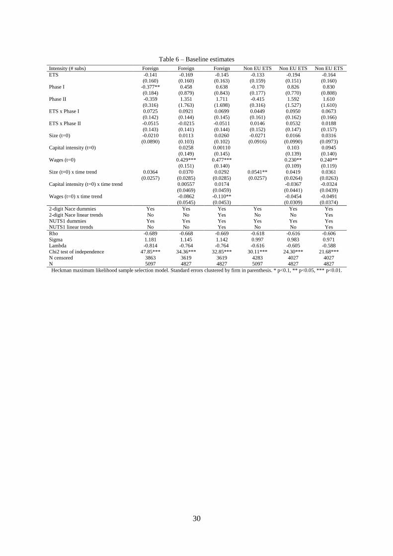
30
Table 6 – Baseline estimates
Intensity (# subs) Foreign Foreign Foreign Non EU ETS Non EU ETS Non EU ETS
ETS -0.141 -0.169 -0.145 -0.133 -0.194 -0.164 (0.160) (0.160) (0.163) (0.159) (0.151) (0.160)
Phase I -0.377** 0.458 0.638 -0.170 0.826 0.830
(0.184) (0.879) (0.843) (0.177) (0.770) (0.808) Phase II -0.359 1.351 1.711 -0.415 1.592 1.610
(0.316) (1.763) (1.698) (0.316) (1.527) (1.610)
ETS x Phase I 0.0725 0.0921 0.0699 0.0449 0.0950 0.0673 (0.142) (0.144) (0.145) (0.161) (0.162) (0.166)
ETS x Phase II -0.0515 -0.0215 -0.0511 0.0146 0.0532 0.0188
(0.143) (0.141) (0.144) (0.152) (0.147) (0.157) Size (t=0) -0.0210 0.0113 0.0260 -0.0271 0.0166 0.0316
(0.0890) (0.103) (0.102) (0.0916) (0.0990) (0.0973) Capital intensity (t=0) 0.0258 0.00110 0.103 0.0945
(0.149) (0.145) (0.139) (0.140)
Wages (t=0) 0.429*** 0.477*** 0.230** 0.240** (0.151) (0.140) (0.109) (0.119)
Size (t=0) x time trend 0.0364 0.0370 0.0292 0.0541** 0.0419 0.0361
(0.0257) (0.0285) (0.0285) (0.0257) (0.0264) (0.0263) Capital intensity (t=0) x time trend 0.00557 0.0174 -0.0367 -0.0324
(0.0469) (0.0459) (0.0441) (0.0439)
Wages (t=0) x time trend -0.0862 -0.110** -0.0454 -0.0491 (0.0545) (0.0453) (0.0309) (0.0374)
2-digit Nace dummies Yes Yes Yes Yes Yes Yes
2-digit Nace linear trends No No Yes No No Yes
NUTS1 dummies Yes Yes Yes Yes Yes Yes NUTS1 linear trends No No Yes No No Yes
Rho -0.689 -0.668 -0.669 -0.618 -0.616 -0.606
Sigma 1.181 1.145 1.142 0.997 0.983 0.971 Lambda -0.814 -0.764 -0.764 -0.616 -0.605 -0.588
Chi2 test of independence 47.85*** 34.36*** 32.85*** 30.11*** 24.30*** 21.68***
N censored 3863 3619 3619 4283 4027 4027 N 5097 4827 4827 5097 4827 4827
Heckman maximum likelihood sample selection model. Standard errors clustered by firm in parenthesis. * p<0.1, ** p<0.05, *** p<0.01.

31
Table 7 – Separate effect for sectors exempted from auctioning (all criteria)
Intensity (# subs) Foreign Foreign Foreign Non EU ETS Non EU ETS Non EU ETS
ETS -0.260 -0.225 -0.196 -0.0424 -0.0629 -0.108 (0.297) (0.306) (0.320) (0.288) (0.291) (0.300)
Phase I -0.650** 0.119 0.221 -0.488* 0.576 0.371
(0.300) (0.913) (0.869) (0.282) (0.774) (0.816) Phase II -0.559* 1.058 1.280 -0.280 1.923 1.580
(0.339) (1.782) (1.722) (0.352) (1.510) (1.604)
ETS x Phase I 0.383 0.417 0.392 0.203 0.296 0.352 (0.334) (0.334) (0.343) (0.339) (0.332) (0.346)
ETS x Phase II 0.317 0.344 0.297 -0.0615 -0.103 -0.0186
(0.291) (0.297) (0.321) (0.299) (0.300) (0.320) Leakage sectors -0.279 -0.249 -0.279 -0.0641 -0.0279 -0.177
(0.248) (0.255) (0.275) (0.263) (0.270) (0.294) Leakage sectors x ETS 0.117 0.0359 0.0237 -0.163 -0.217 -0.145
(0.352) (0.361) (0.380) (0.345) (0.350) (0.370)
Leakage sectors x Phase I 0.350 0.363 0.395 0.432 0.440 0.592* (0.292) (0.291) (0.298) (0.275) (0.280) (0.310)
Leakage sectors x Phase II 0.275 0.248 0.290 -0.0790 -0.147 0.0962
(0.183) (0.190) (0.255) (0.236) (0.241) (0.332) Leakage sectors x ETS x Phase I -0.398 -0.418 -0.410 -0.171 -0.237 -0.321
(0.374) (0.375) (0.383) (0.379) (0.375) (0.389)
Leakage sectors x ETS x Phase II -0.473 -0.471 -0.442 0.0956 0.200 0.0813 (0.332) (0.336) (0.367) (0.349) (0.349) (0.380)
Size (t=0) -0.00435 0.0299 0.0400 0.00225 0.0505 0.0652
(0.0864) (0.103) (0.101) (0.0883) (0.0961) (0.0927) Capital intensity (t=0) 0.0219 -0.00800 0.104 0.0833
(0.149) (0.147) (0.142) (0.145)
Wages (t=0) 0.421*** 0.468*** 0.245** 0.256** (0.153) (0.140) (0.109) (0.117)
Size (t=0) x time trend 0.0345 0.0343 0.0282 0.0492* 0.0351 0.0302
(0.0254) (0.0282) (0.0285) (0.0252) (0.0258) (0.0251) Capital intensity (t=0) x time trend 0.00709 0.0211 -0.0371 -0.0265
(0.0463) (0.0460) (0.0435) (0.0442)
Wages (t=0) x time trend -0.0821 -0.105** -0.0504* -0.0538 (0.0542) (0.0447) (0.0301) (0.0357)
2-digit Nace dummies Yes Yes Yes Yes Yes Yes
2-digit Nace linear trends No No Yes No No Yes
NUTS1 dummies Yes Yes Yes Yes Yes Yes NUTS1 linear trends No No Yes No No Yes
Rho -0.665 -0.644 -0.649 -0.582 -0.586 -0.576
Sigma 1.158 1.123 1.121 0.972 0.961 0.949 Lambda -0.770 -0.723 -0.727 -0.566 -0.563 -0.546
Chi2 test of independence 42.34*** 28.48*** 27.46*** 23.44*** 19.17*** 17.16***
N censored 3863 3619 3619 4283 4027 4027 N 5097 4827 4827 5097 4827 4827
Heckman maximum likelihood sample selection model. Standard errors clustered by firm in parenthesis. * p<0.1, ** p<0.05, *** p<0.01.

32
Table 8 – Separate effect for sectors exempted from auctioning (trade criterion)
Intensity (# subs) Foreign Foreign Foreign Non EU ETS Non EU ETS Non EU ETS
ETS 0.0540 0.0535 0.113 0.237 0.191 0.274 (0.230) (0.231) (0.239) (0.255) (0.248) (0.263)
Phase I -0.338* 0.488 0.677 -0.0521 1.017 0.984
(0.202) (0.887) (0.841) (0.192) (0.759) (0.779) Phase II -0.213 1.492 1.869 -0.163 2.001 1.946
(0.313) (1.777) (1.697) (0.305) (1.492) (1.529)
ETS x Phase I 0.0648 0.0724 0.0155 -0.129 -0.0641 -0.149 (0.184) (0.188) (0.192) (0.236) (0.236) (0.244)
ETS x Phase II -0.188 -0.142 -0.245 -0.389* -0.366 -0.506**
(0.198) (0.197) (0.214) (0.235) (0.233) (0.256) Leakage sectors -0.265 -0.286 -0.279 -0.142 -0.144 -0.140
(0.207) (0.206) (0.211) (0.209) (0.212) (0.228) Leakage sectors x ETS -0.405 -0.453 -0.544 -0.711** -0.727** -0.850**
(0.329) (0.326) (0.335) (0.328) (0.328) (0.341)
Leakage sectors x Phase I 0.0874 0.115 0.103 -0.0713 -0.0601 -0.0632 (0.178) (0.176) (0.178) (0.183) (0.184) (0.197)
Leakage sectors x Phase II -0.0501 -0.0417 -0.0637 -0.179 -0.190 -0.195
(0.150) (0.148) (0.186) (0.154) (0.159) (0.214) Leakage sectors x ETS x Phase I -0.0304 -0.0167 0.0716 0.323 0.294 0.419
(0.270) (0.269) (0.274) (0.307) (0.306) (0.307)
Leakage sectors x ETS x Phase II 0.306 0.261 0.449 0.822*** 0.845*** 1.089*** (0.288) (0.287) (0.310) (0.305) (0.315) (0.332)
Size (t=0) 0.0155 0.0510 0.0700 0.0209 0.0654 0.0900
(0.0871) (0.103) (0.101) (0.0856) (0.0927) (0.0922) Capital intensity (t=0) 0.0166 -0.0103 0.110 0.0886
(0.143) (0.138) (0.134) (0.132)
Wages (t=0) 0.436*** 0.481*** 0.227** 0.235** (0.150) (0.135) (0.102) (0.107)
Size (t=0) x time trend 0.0263 0.0268 0.0176 0.0392 0.0264 0.0172
(0.0258) (0.0290) (0.0291) (0.0249) (0.0260) (0.0255) Capital intensity (t=0) x time trend 0.00573 0.0191 -0.0440 -0.0318
(0.0471) (0.0460) (0.0454) (0.0437)
Wages (t=0) x time trend -0.0862 -0.108** -0.0439 -0.0459 (0.0544) (0.0437) (0.0290) (0.0335)
2-digit Nace dummies Yes Yes Yes Yes Yes Yes
2-digit Nace linear trends No No Yes No No Yes
NUTS1 dummies Yes Yes Yes Yes Yes Yes NUTS1 linear trends No No Yes No No Yes
Rho -0.693 -0.666 -0.665 -0.617 -0.611 -0.595
Sigma 1.172 1.132 1.127 0.982 0.967 0.949 Lambda -0.812 -0.754 -0.749 -0.607 -0.592 -0.565
Chi2 test of independence 45.11*** 31.92*** 29.66*** 27.93*** 21.95*** 18.32***
N censored 3863 3619 3619 4283 4027 4027 N 5097 4827 4827 5097 4827 4827
Heckman maximum likelihood sample selection model. Standard errors clustered by firm in parenthesis. * p<0.1, ** p<0.05, *** p<0.01.

33
Table 9 – Separate effect for sectors exempted from auctioning (trade >10%)
Intensity (# subs) Foreign Foreign Foreign Non EU ETS Non EU ETS Non EU ETS
ETS -0.115 -0.126 -0.0723 0.0118 -0.0529 0.00522 (0.292) (0.286) (0.293) (0.310) (0.292) (0.296)
Phase I -0.539** 0.195 0.275 -0.475** 0.530 0.359
(0.222) (0.870) (0.783) (0.234) (0.705) (0.680) Phase II -0.490 1.084 1.247 -0.391 1.670 1.346
(0.309) (1.739) (1.589) (0.313) (1.398) (1.359)
ETS x Phase I 0.224 0.266 0.216 0.0990 0.205 0.152 (0.253) (0.253) (0.259) (0.292) (0.288) (0.295)
ETS x Phase II 0.0141 0.000446 -0.0874 -0.362 -0.339 -0.417
(0.281) (0.275) (0.286) (0.302) (0.285) (0.292) Leakage sectors -0.354 -0.335 -0.355 -0.424* -0.430* -0.487*
(0.226) (0.227) (0.239) (0.235) (0.237) (0.251) Leakage sectors x ETS -0.0769 -0.102 -0.152 -0.288 -0.287 -0.357
(0.340) (0.340) (0.346) (0.343) (0.331) (0.328)
Leakage sectors x Phase I 0.264 0.287 0.306 0.457* 0.483** 0.542** (0.220) (0.220) (0.217) (0.234) (0.240) (0.250)
Leakage sectors x Phase II 0.254 0.200 0.232 0.0294 0.0225 0.137
(0.182) (0.180) (0.208) (0.202) (0.203) (0.244) Leakage sectors x ETS x Phase I -0.228 -0.262 -0.217 -0.0694 -0.162 -0.101
(0.311) (0.311) (0.313) (0.343) (0.341) (0.340)
Leakage sectors x ETS x Phase II -0.0733 -0.0106 0.0834 0.587* 0.620* 0.731** (0.323) (0.319) (0.330) (0.350) (0.336) (0.334)
Size (t=0) -0.00360 0.0277 0.0387 -0.00261 0.0374 0.0566
(0.0875) (0.104) (0.102) (0.0849) (0.0924) (0.0907) Capital intensity (t=0) 0.0000663 -0.0380 0.0673 0.0296
(0.143) (0.137) (0.121) (0.115)
Wages (t=0) 0.416*** 0.462*** 0.235** 0.246** (0.147) (0.132) (0.101) (0.105)
Size (t=0) x time trend 0.0327 0.0333 0.0275 0.0504** 0.0370 0.0309
(0.0257) (0.0286) (0.0286) (0.0245) (0.0255) (0.0243) Capital intensity (t=0) x time trend 0.00921 0.0278 -0.0353 -0.0150
(0.0462) (0.0445) (0.0421) (0.0389)
Wages (t=0) x time trend -0.0823 -0.105** -0.0487* -0.0517 (0.0539) (0.0430) (0.0289) (0.0331)
2-digit Nace dummies Yes Yes Yes Yes Yes Yes
2-digit Nace linear trends No No Yes No No Yes
NUTS1 dummies Yes Yes Yes Yes Yes Yes NUTS1 linear trends No No Yes No No Yes
Rho -0.677 -0.654 -0.655 -0.601 -0.613 -0.595
Sigma 1.164 1.129 1.125 0.971 0.965 0.946 Lambda -0.788 -0.739 -0.737 -0.584 -0.591 -0.563
Chi2 test of independence 41.71*** 28.62*** 26.77*** 22.97*** 19.90*** 16.13***
N censored 3863 3619 3619 4283 4027 4027 N 5097 4827 4827 5097 4827 4827
Heckman maximum likelihood sample selection model. Standard errors clustered by firm in parenthesis. * p<0.1, ** p<0.05, *** p<0.01.

34
Figure 4 - Trends in allocated and verified emissions for 'leakage' and 'non-leakage' sectors (in billion
tonnes of CO2-equivalent - all EU ETS plants. Source. European Commission) 6
00
800
100
01
20
01
40
0
2004 2006 2008 2010 2012
Allocated 'no-leak' Verified 'no-leak'
Allocated 'leak' Verified 'no-leak'

35
Appendix A - Results for selection equations
Table 10 – Baseline estimates (selection equation)
Selection (Has subs=1) Foreign Foreign Foreign Non EU ETS Non EU ETS Non EU ETS
ETS 0.0510 0.0167 0.0159 -0.0996 -0.121 -0.128 (0.121) (0.125) (0.124) (0.128) (0.131) (0.131)
Phase I 0.336** 0.0884 -0.149 -0.0419 -0.0272 -0.364
(0.134) (0.351) (0.455) (0.143) (0.406) (0.519) Phase II 0.717*** 0.187 -0.297 0.319 0.348 -0.330
(0.239) (0.706) (0.919) (0.241) (0.810) (1.049)
ETS x Phase I -0.0809 -0.0511 -0.0503 -0.0677 -0.0820 -0.0762 (0.105) (0.108) (0.107) (0.145) (0.151) (0.152)
ETS x Phase II -0.146 -0.115 -0.114 -0.120 -0.108 -0.101
(0.0985) (0.102) (0.0998) (0.113) (0.118) (0.116) Size (t=0) 0.519*** 0.543*** 0.534*** 0.356*** 0.380*** 0.362***
(0.0656) (0.0756) (0.0772) (0.0624) (0.0714) (0.0756)
Capital intensity (t=0) 0.120 0.0930 0.0595 0.0412
(0.102) (0.0969) (0.104) (0.106)
Wages (t=0) -0.00268 -0.00258 0.129 0.120
(0.0851) (0.0924) (0.131) (0.131) Size (t=0) x time trend -0.0434* -0.0394* -0.0341 -0.0112 -0.00948 -0.000103
(0.0228) (0.0238) (0.0260) (0.0221) (0.0232) (0.0275)
Capital intensity (t=0) x time trend 0.00115 0.0155 0.0135 0.0237 (0.0222) (0.0243) (0.0250) (0.0300)
Wages (t=0) x time trend 0.0224 0.0217 -0.0174 -0.0135
(0.0220) (0.0270) (0.0299) (0.0345) Dummy for IT subs 0.734*** 0.726*** 0.738*** 0.618*** 0.610*** 0.620***
(0.118) (0.129) (0.128) (0.130) (0.139) (0.141)
Dummy for IT subs x Phase I 0.0530 0.00843 -0.00394 0.0954 0.0792 0.0696 (0.113) (0.121) (0.121) (0.144) (0.155) (0.155)
Dummy for IT subs x Phase II -0.0331 -0.0732 -0.0881 0.0279 0.0246 0.00896
(0.123) (0.134) (0.135) (0.134) (0.145) (0.146)
2-digit Nace dummies Yes Yes Yes Yes Yes Yes
2-digit Nace linear trends No No Yes No No Yes
NUTS1 dummies Yes Yes Yes Yes Yes Yes NUTS1 linear trends No No Yes No No Yes
Rho -0.689 -0.668 -0.669 -0.618 -0.616 -0.606
Sigma 1.181 1.145 1.142 0.997 0.983 0.971
Lambda -0.814 -0.764 -0.764 -0.616 -0.605 -0.588 Chi2 test of independence 47.85*** 34.36*** 32.85*** 30.11*** 24.30*** 21.68***
N censored 3863 3619 3619 4283 4027 4027 N 5097 4827 4827 5097 4827 4827
Heckman maximum likelihood sample selection model. Standard errors clustered by firm in parenthesis. * p<0.1, ** p<0.05, *** p<0.01.

36
Table 11 – Separate effect for sectors exempted from auctioning (all criteria, selection equation)
Selection (Has subs=1) Foreign Foreign Foreign Non EU ETS Non EU ETS Non EU ETS
ETS 0.322 0.331 0.322 0.229 0.290 0.344 (0.267) (0.283) (0.281) (0.261) (0.273) (0.265)
Phase I 0.610*** 0.480 0.324 0.444* 0.546 0.412
(0.214) (0.360) (0.432) (0.263) (0.439) (0.527) Phase II 0.958*** 0.643 0.320 0.617** 0.784 0.503
(0.273) (0.669) (0.892) (0.305) (0.801) (1.060)
ETS x Phase I -0.189 -0.191 -0.182 -0.365 -0.435 -0.489 (0.285) (0.296) (0.294) (0.355) (0.363) (0.352)
ETS x Phase II -0.305 -0.313 -0.293 -0.365 -0.347 -0.459
(0.296) (0.310) (0.311) (0.343) (0.361) (0.317) Leakage sectors 0.118 0.248 0.268 0.108 0.212 0.329
(0.226) (0.243) (0.251) (0.234) (0.253) (0.267) Leakage sectors x ETS -0.341 -0.389 -0.377 -0.415 -0.510* -0.577*
(0.300) (0.316) (0.313) (0.297) (0.310) (0.302)
Leakage sectors x Phase I -0.333 -0.353 -0.369* -0.571** -0.587** -0.700** (0.222) (0.229) (0.221) (0.286) (0.292) (0.282)
Leakage sectors x Phase II -0.292 -0.304 -0.340 -0.339 -0.325 -0.551**
(0.223) (0.231) (0.230) (0.268) (0.279) (0.267) Leakage sectors x ETS x Phase I 0.120 0.158 0.148 0.323 0.394 0.461
(0.307) (0.318) (0.314) (0.389) (0.399) (0.388)
Leakage sectors x ETS x Phase II 0.200 0.245 0.218 0.298 0.289 0.424 (0.312) (0.326) (0.326) (0.359) (0.376) (0.333)
Size (t=0) 0.512*** 0.541*** 0.541*** 0.355*** 0.380*** 0.370***
(0.0661) (0.0773) (0.0792) (0.0632) (0.0736) (0.0783) Capital intensity (t=0) 0.126 0.105 0.0549 0.0488
(0.103) (0.100) (0.108) (0.111)
Wages (t=0) 0.00375 0.00231 0.134 0.124 (0.0852) (0.0923) (0.134) (0.133)
Size (t=0) x time trend -0.0449** -0.0419* -0.0413 -0.0134 -0.0127 -0.00705
(0.0221) (0.0233) (0.0255) (0.0215) (0.0227) (0.0269) Capital intensity (t=0) x time trend -0.00271 0.00803 0.0107 0.0146
(0.0216) (0.0246) (0.0248) (0.0306)
Wages (t=0) x time trend 0.0179 0.0181 -0.0207 -0.0161 (0.0210) (0.0259) (0.0300) (0.0340)
Dummy for IT subs 0.712*** 0.712*** 0.725*** 0.582*** 0.578*** 0.594***
(0.120) (0.129) (0.129) (0.132) (0.140) (0.143)
Dummy for IT subs x Phase I 0.0600 0.0161 0.00261 0.101 0.0894 0.0739
(0.112) (0.119) (0.119) (0.146) (0.155) (0.156)
Dummy for IT subs x Phase II -0.0112 -0.0555 -0.0683 0.0478 0.0464 0.0308 (0.123) (0.132) (0.133) (0.138) (0.148) (0.149)
2-digit Nace dummies Yes Yes Yes Yes Yes Yes
2-digit Nace linear trends No No Yes No No Yes NUTS1 dummies Yes Yes Yes Yes Yes Yes
NUTS1 linear trends No No Yes No No Yes
Rho -0.665 -0.644 -0.649 -0.582 -0.586 -0.576
Sigma 1.158 1.123 1.121 0.972 0.961 0.949 Lambda -0.770 -0.723 -0.727 -0.566 -0.563 -0.546
Chi2 test of independence 42.34*** 28.48*** 27.46*** 23.44*** 19.17*** 17.16***
N censored 3863 3619 3619 4283 4027 4027 N 5097 4827 4827 5097 4827 4827
Heckman maximum likelihood sample selection model. Standard errors clustered by firm in parenthesis. * p<0.1, ** p<0.05, *** p<0.01.

37
Table 12 – Separate effect for sectors exempted from auctioning (trade criterion, selection equation)
Selection (Has subs=1) Foreign Foreign Foreign Non EU ETS Non EU ETS Non EU ETS
ETS 0.0536 -0.0215 -0.0349 -0.207 -0.261 -0.276 (0.154) (0.161) (0.161) (0.168) (0.174) (0.172)
Phase I 0.326** 0.111 -0.139 -0.0614 -0.0796 -0.363
(0.141) (0.365) (0.454) (0.161) (0.403) (0.507) Phase II 0.685*** 0.202 -0.303 0.266 0.217 -0.349
(0.245) (0.732) (0.923) (0.243) (0.804) (1.033)
ETS x Phase I -0.0486 -0.0114 0.00159 0.0395 0.0107 0.0243 (0.122) (0.123) (0.125) (0.194) (0.204) (0.206)
ETS x Phase II -0.125 -0.0836 -0.0565 -0.0427 -0.0194 0.00369
(0.118) (0.123) (0.129) (0.148) (0.158) (0.158) Leakage sectors 0.231 0.264 0.249 0.284 0.300 0.275
(0.169) (0.168) (0.175) (0.181) (0.184) (0.193) Leakage sectors x ETS -0.0522 0.0527 0.0912 0.194 0.265 0.299
(0.252) (0.257) (0.258) (0.258) (0.264) (0.266)
Leakage sectors x Phase I -0.0103 -0.0397 -0.0212 -0.0608 -0.0733 -0.0455 (0.114) (0.116) (0.114) (0.159) (0.161) (0.160)
Leakage sectors x Phase II 0.0313 0.0388 0.0702 -0.0699 -0.0599 -0.0112
(0.108) (0.110) (0.120) (0.105) (0.108) (0.131) Leakage sectors x ETS x Phase I -0.0804 -0.0883 -0.126 -0.218 -0.176 -0.210
(0.223) (0.230) (0.228) (0.269) (0.281) (0.285)
Leakage sectors x ETS x Phase II -0.0591 -0.0897 -0.171 -0.154 -0.180 -0.248 (0.203) (0.210) (0.214) (0.215) (0.226) (0.234)
Size (t=0) 0.513*** 0.535*** 0.526*** 0.336*** 0.360*** 0.348***
(0.0666) (0.0770) (0.0770) (0.0623) (0.0731) (0.0766) Capital intensity (t=0) 0.134 0.109 0.0711 0.0586
(0.101) (0.0962) (0.103) (0.105)
Wages (t=0) -0.0106 -0.0113 0.111 0.108 (0.0836) (0.0902) (0.125) (0.124)
Size (t=0) x time trend -0.0418* -0.0371 -0.0311 -0.00429 -0.00250 0.00418
(0.0239) (0.0249) (0.0259) (0.0229) (0.0241) (0.0275) Capital intensity (t=0) x time trend -0.000665 0.0129 0.0125 0.0198
(0.0221) (0.0246) (0.0245) (0.0295)
Wages (t=0) x time trend 0.0218 0.0215 -0.0127 -0.0116 (0.0233) (0.0272) (0.0292) (0.0332)
Dummy for IT subs 0.734*** 0.727*** 0.739*** 0.627*** 0.620*** 0.626***
(0.118) (0.130) (0.130) (0.132) (0.140) (0.143)
Dummy for IT subs x Phase I 0.0581 0.0124 0.000731 0.0935 0.0749 0.0702
(0.113) (0.121) (0.121) (0.142) (0.153) (0.155)
Dummy for IT subs x Phase II -0.0251 -0.0689 -0.0840 0.0205 0.0156 0.00763 (0.124) (0.135) (0.135) (0.133) (0.143) (0.145)
2-digit Nace dummies Yes Yes Yes Yes Yes Yes
2-digit Nace linear trends No No Yes No No Yes NUTS1 dummies Yes Yes Yes Yes Yes Yes
NUTS1 linear trends No No Yes No No Yes
Rho -0.693 -0.666 -0.665 -0.617 -0.611 -0.595
Sigma 1.172 1.132 1.127 0.982 0.967 0.949 Lambda -0.812 -0.754 -0.749 -0.607 -0.592 -0.565
Chi2 test of independence 45.11*** 31.92*** 29.66*** 27.93*** 21.95*** 18.32***
N censored 3863 3619 3619 4283 4027 4027 N 5097 4827 4827 5097 4827 4827
Heckman maximum likelihood sample selection model. Standard errors clustered by firm in parenthesis. * p<0.1, ** p<0.05, *** p<0.01.

38
Table 13 – Separate effect for sectors exempted from auctioning (trade >10%, selection equation)
Selection (Has subs=1) Foreign Foreign Foreign Non EU ETS Non EU ETS Non EU ETS
ETS 0.156 0.126 0.103 0.0239 0.0181 0.0286 (0.194) (0.203) (0.203) (0.198) (0.206) (0.203)
Phase I 0.393*** 0.224 0.00984 0.155 0.217 -0.0587
(0.148) (0.326) (0.416) (0.178) (0.387) (0.492) Phase II 0.828*** 0.411 -0.0210 0.371 0.471 -0.0872
(0.225) (0.650) (0.872) (0.238) (0.752) (1.014)
ETS x Phase I -0.0331 -0.0353 -0.0133 -0.0612 -0.104 -0.116 (0.185) (0.193) (0.193) (0.242) (0.247) (0.243)
ETS x Phase II -0.222 -0.182 -0.138 -0.0485 -0.0355 -0.0587
(0.198) (0.206) (0.211) (0.230) (0.239) (0.225) Leakage sectors 0.277* 0.316* 0.299* 0.310* 0.328* 0.356**
(0.159) (0.165) (0.165) (0.169) (0.176) (0.177) Leakage sectors x ETS -0.156 -0.160 -0.123 -0.174 -0.196 -0.218
(0.251) (0.262) (0.261) (0.259) (0.266) (0.263)
Leakage sectors x Phase I -0.110 -0.130 -0.113 -0.300 -0.313 -0.341* (0.149) (0.154) (0.145) (0.211) (0.213) (0.204)
Leakage sectors x Phase II -0.228 -0.194 -0.165 -0.134 -0.127 -0.179
(0.155) (0.160) (0.154) (0.170) (0.173) (0.153) Leakage sectors x ETS x Phase I -0.0848 -0.0341 -0.0678 -0.0395 0.00212 0.0265
(0.227) (0.234) (0.231) (0.301) (0.308) (0.305)
Leakage sectors x ETS x Phase II 0.111 0.0929 0.0233 -0.126 -0.130 -0.0893 (0.225) (0.235) (0.242) (0.258) (0.268) (0.256)
Size (t=0) 0.509*** 0.536*** 0.532*** 0.347*** 0.372*** 0.359***
(0.0654) (0.0755) (0.0770) (0.0621) (0.0716) (0.0759) Capital intensity (t=0) 0.136 0.114 0.0694 0.0615
(0.0996) (0.0962) (0.103) (0.105)
Wages (t=0) 0.00414 0.00316 0.129 0.116 (0.0849) (0.0926) (0.128) (0.128)
Size (t=0) x time trend -0.0399* -0.0368 -0.0341 -0.00799 -0.00697 0.000737
(0.0232) (0.0241) (0.0259) (0.0223) (0.0234) (0.0273) Capital intensity (t=0) x time trend -0.00161 0.00985 0.0110 0.0161
(0.0216) (0.0246) (0.0246) (0.0304)
Wages (t=0) x time trend 0.0197 0.0195 -0.0178 -0.0121 (0.0215) (0.0264) (0.0289) (0.0339)
Dummy for IT subs 0.739*** 0.733*** 0.744*** 0.613*** 0.606*** 0.614***
(0.120) (0.131) (0.132) (0.131) (0.140) (0.144)
Dummy for IT subs x Phase I 0.0483 0.00557 -0.00527 0.0811 0.0662 0.0588
(0.115) (0.122) (0.123) (0.145) (0.154) (0.156)
Dummy for IT subs x Phase II -0.0326 -0.0736 -0.0864 0.0372 0.0376 0.0242 (0.125) (0.137) (0.137) (0.137) (0.147) (0.150)
2-digit Nace dummies Yes Yes Yes Yes Yes Yes
2-digit Nace linear trends No No Yes No No Yes NUTS1 dummies Yes Yes Yes Yes Yes Yes
NUTS1 linear trends No No Yes No No Yes
Rho -0.677 -0.654 -0.655 -0.601 -0.613 -0.595
Sigma 1.164 1.129 1.125 0.971 0.965 0.946 Lambda -0.788 -0.739 -0.737 -0.584 -0.591 -0.563
Chi2 test of independence 41.71*** 28.62*** 26.77*** 22.97*** 19.90*** 16.13***
N censored 3863 3619 3619 4283 4027 4027 N 5097 4827 4827 5097 4827 4827
Heckman maximum likelihood sample selection model. Standard errors clustered by firm in parenthesis. * p<0.1, ** p<0.05, *** p<0.01.

39
Appendix B - Results for subsidiaries in EU ETS countries
Table 14 – Baseline estimates
Intensity (# subs) ETS ETS ETS
ETS -0.0733 -0.110 -0.0678 (0.166) (0.163) (0.167)
Phase I -0.488** 0.447 0.722
(0.195) (1.060) (0.982) Phase II -0.666* 1.252 1.799
(0.354) (2.127) (1.969)
ETS x Phase I -0.0873 -0.0406 -0.0823 (0.130) (0.133) (0.133)
ETS x Phase II 0.0648 0.106 0.0300
(0.158) (0.154) (0.156) Size (t=0) -0.102 -0.0362 -0.0230
(0.0898) (0.107) (0.109)
Capital intensity (t=0) 0.176 0.169 (0.175) (0.170)
Wages (t=0) 0.299** 0.339***
(0.130) (0.126) Size (t=0) x time trend 0.0440 0.0313 0.0266
(0.0280) (0.0330) (0.0325)
Capital intensity (t=0) x time trend -0.0549 -0.0510 (0.0592) (0.0567)
Wages (t=0) x time trend -0.0196 -0.0392
(0.0511) (0.0456)
2-digit Nace dummies Yes Yes Yes
2-digit Nace linear trends No No Yes
NUTS1 dummies Yes Yes Yes NUTS1 linear trends No No Yes
Rho -0.669 -0.656 -0.656
Sigma 1.060 1.019 1.013
Lambda -0.709 -0.668 -0.664 Chi2 test of independence 42.00*** 29.71*** 26.01***
N censored 4114 3861 3861
N 5097 4827 4827
Heckman maximum likelihood sample selection model. Standard errors clustered by firm
in parenthesis. * p<0.1, ** p<0.05, *** p<0.01.

40
Table 15 – Separate effect for sectors exempted from auctioning (all criteria)
Intensity (# subs) ETS ETS ETS
ETS -0.0834 -0.0397 -0.0674 (0.291) (0.306) (0.327)
Phase I -0.611*** 0.257 0.0204
(0.224) (1.104) (1.038) Phase II -0.728** 1.071 0.601
(0.355) (2.203) (2.068)
ETS x Phase I -0.139 -0.0976 -0.0695 (0.249) (0.264) (0.284)
ETS x Phase II -0.0757 -0.0564 0.0123
(0.256) (0.273) (0.313) Leakage sectors -0.413* -0.354 -0.619**
(0.236) (0.237) (0.267) Leakage sectors x ETS -0.0253 -0.126 -0.0415
(0.348) (0.355) (0.375)
Leakage sectors x Phase I 0.163 0.162 0.413** (0.186) (0.189) (0.204)
Leakage sectors x Phase II 0.100 0.0750 0.570**
(0.180) (0.184) (0.248) Leakage sectors x ETS x Phase I 0.0784 0.0836 -0.00175
(0.289) (0.301) (0.317)
Leakage sectors x ETS x Phase II 0.182 0.207 0.0290 (0.326) (0.332) (0.374)
Size (t=0) -0.0834 -0.0185 -0.0126
(0.0832) (0.103) (0.104) Capital intensity (t=0) 0.162 0.121
(0.177) (0.171)
Wages (t=0) 0.284** 0.312** (0.132) (0.125)
Size (t=0) x time trend 0.0427 0.0298 0.0305
(0.0270) (0.0328) (0.0314) Capital intensity (t=0) x time trend -0.0514 -0.0305
(0.0601) (0.0573)
Wages (t=0) x time trend -0.0168 -0.0304 (0.0516) (0.0450)
2-digit Nace dummies Yes Yes Yes
2-digit Nace linear trends No No Yes
NUTS1 dummies Yes Yes Yes NUTS1 linear trends No No Yes
Rho -0.633 -0.618 -0.611
Sigma 1.029 0.991 0.979 Lambda -0.651 -0.613 -0.598
Chi2 test of independence 34.11*** 23.25*** 20.01***
N censored 4114 3861 3861 N 5097 4827 4827
Heckman maximum likelihood sample selection model. Standard errors clustered by firm
in parenthesis. * p<0.1, ** p<0.05, *** p<0.01.

41
Table 16 – Separate effect for sectors exempted from auctioning (trade criterion)
Intensity (# subs) ETS ETS ETS
ETS 0.0419 0.0391 0.114 (0.240) (0.236) (0.247)
Phase I -0.444** 0.455 0.727
(0.206) (1.072) (0.990) Phase II -0.543 1.306 1.848
(0.367) (2.144) (1.980)
ETS x Phase I -0.113 -0.0918 -0.163 (0.162) (0.170) (0.174)
ETS x Phase II -0.00160 0.0370 -0.106
(0.217) (0.217) (0.230) Leakage sectors -0.382* -0.372* -0.366
(0.229) (0.224) (0.237) Leakage sectors x ETS -0.176 -0.244 -0.319
(0.335) (0.333) (0.339)
Leakage sectors x Phase I 0.119 0.108 0.0978 (0.161) (0.159) (0.172)
Leakage sectors x Phase II 0.0725 0.0358 0.00793
(0.167) (0.166) (0.214) Leakage sectors x ETS x Phase I -0.00955 0.0378 0.105
(0.252) (0.254) (0.253)
Leakage sectors x ETS x Phase II 0.120 0.121 0.279 (0.322) (0.324) (0.327)
Size (t=0) -0.0727 -0.0104 0.00508
(0.0926) (0.110) (0.111) Capital intensity (t=0) 0.146 0.137
(0.168) (0.163)
Wages (t=0) 0.314** 0.350*** (0.131) (0.123)
Size (t=0) x time trend 0.0331 0.0216 0.0164
(0.0291) (0.0347) (0.0339) Capital intensity (t=0) x time trend -0.0491 -0.0440
(0.0580) (0.0552)
Wages (t=0) x time trend -0.0230 -0.0405 (0.0524) (0.0449)
2-digit Nace dummies Yes Yes Yes
2-digit Nace linear trends No No Yes
NUTS1 dummies Yes Yes Yes NUTS1 linear trends No No Yes
Rho -0.685 -0.675 -0.674
Sigma 1.059 1.019 1.011 Lambda -0.726 -0.688 -0.681
Chi2 test of independence 38.45*** 27.82*** 23.69***
N censored 4114 3861 3861 N 5097 4827 4827
Heckman maximum likelihood sample selection model. Standard errors clustered by firm
in parenthesis. * p<0.1, ** p<0.05, *** p<0.01.

42
Table 17 – Separate effect for sectors exempted from auctioning (trade >10%)
Intensity (# subs) ETS ETS ETS
ETS 0.139 0.135 0.143 (0.311) (0.306) (0.317)
Phase I -0.448** 0.409 0.415
(0.205) (1.029) (0.907) Phase II -0.648* 1.176 1.203
(0.343) (2.054) (1.809)
ETS x Phase I -0.295 -0.246 -0.255 (0.221) (0.228) (0.244)
ETS x Phase II -0.149 -0.165 -0.199
(0.299) (0.299) (0.314) Leakage sectors -0.211 -0.167 -0.297
(0.232) (0.227) (0.248) Leakage sectors x ETS -0.334 -0.376 -0.323
(0.352) (0.351) (0.354)
Leakage sectors x Phase I -0.0342 -0.0305 0.0907 (0.166) (0.164) (0.172)
Leakage sectors x Phase II 0.00642 -0.0748 0.140
(0.189) (0.184) (0.221) Leakage sectors x ETS x Phase I 0.299 0.294 0.243
(0.274) (0.277) (0.282)
Leakage sectors x ETS x Phase II 0.339 0.413 0.348 (0.351) (0.352) (0.345)
Size (t=0) -0.0916 -0.0307 -0.0222
(0.0902) (0.108) (0.111) Capital intensity (t=0) 0.138 0.107
(0.167) (0.158)
Wages (t=0) 0.291** 0.322*** (0.124) (0.118)
Size (t=0) x time trend 0.0420 0.0299 0.0270
(0.0284) (0.0333) (0.0325) Capital intensity (t=0) x time trend -0.0492 -0.0335
(0.0574) (0.0541)
Wages (t=0) x time trend -0.0192 -0.0345 (0.0496) (0.0435)
2-digit Nace dummies Yes Yes Yes
2-digit Nace linear trends No No Yes
NUTS1 dummies Yes Yes Yes NUTS1 linear trends No No Yes
Rho -0.668 -0.654 -0.654
Sigma 1.048 1.010 1.002 Lambda -0.700 -0.660 -0.656
Chi2 test of independence 34.08*** 23.21*** 19.32***
N censored 4114 3861 3861 N 5097 4827 4827
Heckman maximum likelihood sample selection model. Standard errors clustered by firm
in parenthesis. * p<0.1, ** p<0.05, *** p<0.01.

43
Appendix C - Results based on kernel matching
Table 18 – Baseline estimates (matching based on kernel)
Intensity (# subs) Foreign Foreign Foreign Non EU ETS Non EU ETS Non EU ETS
ETS -0.109 -0.128 -0.113 -0.0487 -0.0981 -0.0567 (0.169) (0.165) (0.169) (0.187) (0.176) (0.186)
Phase I -0.425** 1.166 1.023 -0.188 1.117 1.039
(0.196) (0.946) (0.890) (0.192) (0.831) (0.804) Phase II -0.518 2.694 2.403 -0.617* 2.006 1.867
(0.337) (1.896) (1.785) (0.339) (1.615) (1.567)
ETS x Phase I 0.0472 0.0618 0.0457 -0.0507 -0.000168 -0.0370 (0.138) (0.139) (0.141) (0.174) (0.174) (0.180)
ETS x Phase II -0.0374 -0.00129 -0.0153 0.0253 0.0607 0.000972
(0.150) (0.148) (0.151) (0.172) (0.171) (0.177) Size (t=0) -0.0727 -0.0331 -0.0303 -0.0963 -0.0568 -0.0406
(0.0959) (0.110) (0.111) (0.0978) (0.103) (0.105)
Capital intensity (t=0) 0.150 0.109 0.222 0.231 (0.170) (0.170) (0.171) (0.170)
Wages (t=0) 0.389** 0.394** 0.169 0.140
(0.197) (0.194) (0.112) (0.122) Size (t=0) x time trend 0.0475* 0.0429 0.0412 0.0680** 0.0551* 0.0492
(0.0278) (0.0296) (0.0306) (0.0283) (0.0285) (0.0301)
Capital intensity (t=0) x time trend -0.0398 -0.0194 -0.0742 -0.0767 (0.0443) (0.0447) (0.0482) (0.0496)
Wages (t=0) x time trend -0.102 -0.104 -0.0305 -0.0149
(0.0711) (0.0680) (0.0374) (0.0393)
2-digit Nace dummies Yes Yes Yes Yes Yes Yes
2-digit Nace linear trends No No Yes No No Yes
NUTS1 dummies Yes Yes Yes Yes Yes Yes NUTS1 linear trends No No Yes No No Yes
Rho -0.717 -0.698 -0.698 -0.627 -0.632 -0.628
Sigma 1.242 1.206 1.203 1.065 1.052 1.040
Lambda -0.890 -0.841 -0.840 -0.668 -0.665 -0.653 Chi2 test of independence 68.44*** 47.05*** 45.90*** 51.02*** 39.60*** 36.99***
N censored 169025 150045 150045 172748 153565 153565
N 177024 157644 157644 177024 157644 157644
Heckman maximum likelihood sample selection model. Standard errors clustered by firm in parenthesis. * p<0.1, ** p<0.05, *** p<0.01.

44
Table 19 – Separate effect for sectors exempted from auctioning (all criteria, matching based on kernel)
Intensity (# subs) Foreign Foreign Foreign Non EU ETS Non EU ETS Non EU ETS
ETS -0.418 -0.352 -0.301 -0.561 -0.571* -0.488 (0.349) (0.347) (0.368) (0.354) (0.344) (0.326)
Phase I -0.848*** 0.628 0.438 -0.847*** 0.410 0.319
(0.290) (0.922) (0.859) (0.290) (0.823) (0.795) Phase II -0.878** 2.132 1.747 -0.888** 1.670 1.527
(0.397) (1.831) (1.709) (0.431) (1.618) (1.556)
ETS x Phase I 0.578* 0.599* 0.548 0.451 0.544* 0.481 (0.328) (0.336) (0.352) (0.339) (0.317) (0.321)
ETS x Phase II 0.550 0.571 0.490 0.301 0.273 0.152
(0.349) (0.357) (0.398) (0.365) (0.345) (0.344) Leakage sectors -0.359 -0.296 -0.340 -0.745** -0.693** -0.716**
(0.289) (0.276) (0.289) (0.315) (0.290) (0.284) Leakage sectors x ETS 0.357 0.252 0.200 0.535 0.495 0.433
(0.405) (0.405) (0.432) (0.415) (0.414) (0.414)
Leakage sectors x Phase I 0.503* 0.496* 0.536** 0.752*** 0.751*** 0.789*** (0.262) (0.271) (0.273) (0.282) (0.270) (0.291)
Leakage sectors x Phase II 0.435* 0.385 0.465 0.330 0.285 0.337
(0.252) (0.259) (0.283) (0.311) (0.292) (0.333) Leakage sectors x ETS x Phase I -0.649* -0.659* -0.609 -0.529 -0.589 -0.547
(0.361) (0.368) (0.384) (0.385) (0.369) (0.383)
Leakage sectors x ETS x Phase II -0.723* -0.708* -0.615 -0.306 -0.229 -0.139 (0.385) (0.390) (0.437) (0.410) (0.394) (0.415)
Size (t=0) -0.0609 -0.0193 -0.0192 -0.0792 -0.0413 -0.0210
(0.0932) (0.108) (0.109) (0.0918) (0.0975) (0.0976) Capital intensity (t=0) 0.148 0.111 0.218 0.214
(0.170) (0.173) (0.174) (0.177)
Wages (t=0) 0.373* 0.372** 0.155 0.137 (0.192) (0.188) (0.107) (0.116)
Size (t=0) x time trend 0.0464* 0.0415 0.0409 0.0662** 0.0527* 0.0454
(0.0276) (0.0294) (0.0304) (0.0276) (0.0280) (0.0291) Capital intensity (t=0) x time trend -0.0388 -0.0207 -0.0728 -0.0691
(0.0437) (0.0453) (0.0477) (0.0504)
Wages (t=0) x time trend -0.0915 -0.0909 -0.0270 -0.0168 (0.0667) (0.0634) (0.0362) (0.0370)
2-digit Nace dummies Yes Yes Yes Yes Yes Yes
2-digit Nace linear trends No No Yes No No Yes
NUTS1 dummies Yes Yes Yes Yes Yes Yes NUTS1 linear trends No No Yes No No Yes
Rho -0.704 -0.684 -0.686 -0.602 -0.616 -0.611
Sigma 1.228 1.192 1.189 1.043 1.037 1.024 Lambda -0.865 -0.815 -0.815 -0.628 -0.639 -0.625
Chi2 test of independence 69.04*** 44.38*** 43.47*** 45.78*** 36.28*** 33.80***
N censored 169025 150045 150045 172748 153565 153565 N 177024 157644 157644 177024 157644 157644
Heckman maximum likelihood sample selection model. Standard errors clustered by firm in parenthesis. * p<0.1, ** p<0.05, *** p<0.01.

45
Table 20 – Separate effect for sectors exempted from auctioning (trade criterion, matching based on
kernel)
Intensity (# subs) Foreign Foreign Foreign Non EU ETS Non EU ETS Non EU ETS
ETS 0.0455 0.0483 0.112 0.272 0.234 0.313
(0.244) (0.238) (0.247) (0.292) (0.274) (0.290)
Phase I -0.407* 1.118 0.986 -0.140 1.100 0.960 (0.211) (0.936) (0.880) (0.204) (0.780) (0.773)
Phase II -0.426 2.665 2.395 -0.395 2.096 1.836
(0.337) (1.872) (1.761) (0.325) (1.491) (1.466) ETS x Phase I 0.0596 0.0558 -0.00666 -0.159 -0.114 -0.192
(0.179) (0.181) (0.187) (0.243) (0.241) (0.254)
ETS x Phase II -0.120 -0.0735 -0.182 -0.361 -0.341 -0.479* (0.204) (0.203) (0.219) (0.251) (0.251) (0.269)
Leakage sectors -0.340 -0.342 -0.355 -0.243 -0.229 -0.215
(0.221) (0.223) (0.228) (0.253) (0.253) (0.263) Leakage sectors x ETS -0.366 -0.407 -0.538 -0.655* -0.667* -0.784**
(0.352) (0.347) (0.355) (0.372) (0.361) (0.369)
Leakage sectors x Phase I 0.0774 0.0933 0.0986 0.118 0.108 0.0954 (0.168) (0.171) (0.178) (0.245) (0.244) (0.253)
Leakage sectors x Phase II -0.0437 -0.0540 -0.0303 -0.127 -0.166 -0.189
(0.164) (0.169) (0.198) (0.207) (0.209) (0.238) Leakage sectors x ETS x Phase I -0.0745 -0.0369 0.0885 0.135 0.146 0.266
(0.269) (0.270) (0.275) (0.340) (0.341) (0.338)
Leakage sectors x ETS x Phase II 0.200 0.175 0.430 0.807** 0.838** 1.075*** (0.291) (0.287) (0.311) (0.324) (0.327) (0.337)
Size (t=0) -0.0455 -0.00692 0.00291 -0.0496 -0.0171 0.00611
(0.0958) (0.109) (0.110) (0.0945) (0.0976) (0.0993) Capital intensity (t=0) 0.121 0.0732 0.193 0.185
(0.161) (0.160) (0.155) (0.153)
Wages (t=0) 0.395** 0.401** 0.167 0.137 (0.198) (0.194) (0.109) (0.119)
Size (t=0) x time trend 0.0413 0.0375 0.0330 0.0544* 0.0433 0.0362
(0.0282) (0.0297) (0.0307) (0.0279) (0.0276) (0.0282) Capital intensity (t=0) x time trend -0.0355 -0.0119 -0.0699 -0.0633
(0.0435) (0.0439) (0.0452) (0.0462)
Wages (t=0) x time trend -0.102 -0.104 -0.0298 -0.0127 (0.0716) (0.0678) (0.0359) (0.0382)
2-digit Nace dummies Yes Yes Yes Yes Yes Yes
2-digit Nace linear trends No No Yes No No Yes NUTS1 dummies Yes Yes Yes Yes Yes Yes
NUTS1 linear trends No No Yes No No Yes
Rho -0.722 -0.700 -0.699 -0.621 -0.627 -0.611 Sigma 1.234 1.197 1.191 1.046 1.035 1.016
Lambda -0.892 -0.838 -0.833 -0.650 -0.649 -0.621
Chi2 test of independence 60.61*** 42.06*** 40.30*** 45.42*** 36.05*** 31.24*** N censored 169025 150045 150045 172748 153565 153565
N 177024 157644 157644 177024 157644 157644
Heckman maximum likelihood sample selection model. Standard errors clustered by firm in parenthesis. * p<0.1, ** p<0.05, *** p<0.01.

46
Table 21 – Separate effect for sectors exempted from auctioning (trade >10%, matching based on kernel)
Intensity (# subs) Foreign Foreign Foreign Non EU ETS Non EU ETS Non EU ETS
ETS -0.107 -0.0975 -0.0222 -0.110 -0.159 -0.0351 (0.368) (0.354) (0.365) (0.369) (0.341) (0.350)
Phase I -0.705*** 0.754 0.515 -0.583** 0.623 0.437
(0.217) (0.902) (0.817) (0.257) (0.738) (0.703) Phase II -0.707** 2.284 1.799 -0.819** 1.604 1.247
(0.334) (1.817) (1.660) (0.373) (1.438) (1.375)
ETS x Phase I 0.291 0.317 0.245 0.00500 0.0856 -0.0223 (0.265) (0.267) (0.278) (0.314) (0.307) (0.319)
ETS x Phase II 0.0850 0.0801 -0.0351 -0.189 -0.167 -0.353
(0.356) (0.353) (0.375) (0.337) (0.317) (0.332) Leakage sectors -0.436 -0.383 -0.393 -0.839*** -0.835*** -0.833***
(0.297) (0.292) (0.301) (0.279) (0.270) (0.286) Leakage sectors x ETS -0.0712 -0.107 -0.202 -0.0913 -0.0832 -0.225
(0.407) (0.401) (0.418) (0.396) (0.377) (0.378)
Leakage sectors x Phase I 0.410** 0.409* 0.417** 0.525** 0.523** 0.533* (0.206) (0.209) (0.207) (0.265) (0.266) (0.283)
Leakage sectors x Phase II 0.313 0.248 0.271 0.323 0.304 0.328
(0.285) (0.282) (0.297) (0.259) (0.253) (0.287) Leakage sectors x ETS x Phase I -0.343 -0.363 -0.274 -0.0186 -0.0816 0.0389
(0.311) (0.312) (0.322) (0.366) (0.364) (0.370)
Leakage sectors x ETS x Phase II -0.144 -0.0933 0.0672 0.396 0.420 0.641* (0.390) (0.388) (0.422) (0.385) (0.369) (0.377)
Size (t=0) -0.0521 -0.0120 -0.0133 -0.0578 -0.0273 -0.00837
(0.0969) (0.110) (0.112) (0.0878) (0.0925) (0.0918) Capital intensity (t=0) 0.117 0.0565 0.137 0.0887
(0.159) (0.158) (0.138) (0.127)
Wages (t=0) 0.373** 0.378** 0.177* 0.175* (0.188) (0.178) (0.0980) (0.0993)
Size (t=0) x time trend 0.0441 0.0395 0.0398 0.0631** 0.0503* 0.0448*
(0.0290) (0.0305) (0.0315) (0.0262) (0.0265) (0.0263) Capital intensity (t=0) x time trend -0.0354 -0.00609 -0.0655 -0.0397
(0.0430) (0.0439) (0.0431) (0.0426)
Wages (t=0) x time trend -0.0944 -0.0966 -0.0305 -0.0276 (0.0685) (0.0629) (0.0342) (0.0357)
2-digit Nace dummies Yes Yes Yes Yes Yes Yes
2-digit Nace linear trends No No Yes No No Yes
NUTS1 dummies Yes Yes Yes Yes Yes Yes NUTS1 linear trends No No Yes No No Yes
Rho -0.704 -0.681 -0.681 -0.604 -0.629 -0.616
Sigma 1.221 1.186 1.181 1.020 1.022 1.003 Lambda -0.859 -0.808 -0.805 -0.616 -0.643 -0.618
Chi2 test of independence 53.27*** 35.66*** 33.65*** 33.28*** 30.48*** 26.72***
N censored 169025 150045 150045 172748 153565 153565 N 177024 157644 157644 177024 157644 157644
Heckman maximum likelihood sample selection model. Standard errors clustered by firm in parenthesis. * p<0.1, ** p<0.05, *** p<0.01.

47
Appendix D - Selection bias correction based on Semekyna and
Wooldridge (2010)
Table 22 – Baseline estimates (based on Semekyna and Wooldridge, 2010)
Intensity (# subs) OLS
Semekyna and
Wooldridge (2010)
OLS
Semekyna and
Wooldridge (2010)
Foreign Foreign Non EU ETS Non EU ETS
ETS -0.201 -0.163 -0.246 -0.163
(0.161) (0.147) (0.159) (0.152) Phase I 0.442 1.995** 0.582 2.142*
(0.858) (0.939) (0.844) (1.158)
Phase II 1.342 1.906 1.239 2.385 (1.716) (1.738) (1.672) (1.873)
ETS x Phase I 0.0791 0.0544 0.0658 0.0637
(0.131) (0.132) (0.150) (0.149)
ETS x Phase II -0.0693 -0.0412 0.0158 0.0184
(0.130) (0.130) (0.150) (0.161)
Size (t=0) 0.280*** -0.295** 0.191** -0.0630 (0.0927) (0.137) (0.0898) (0.127)
Capital intensity (t=0) 0.0889 -0.0695 0.130 0.0848
(0.152) (0.124) (0.138) (0.129) Wages (t=0) 0.493*** 0.454*** 0.290** 0.216
(0.165) (0.155) (0.136) (0.137)
Size (t=0) x time trend 0.0222 0.0934* 0.0385 0.0783 (0.0268) (0.0495) (0.0263) (0.0527)
Capital intensity (t=0) x time trend 0.0295 0.0349 -0.0156 -0.0155
(0.0463) (0.0442) (0.0436) (0.0408) Wages (t=0) x time trend -0.103** -0.116** -0.0534 -0.0415
(0.0463) (0.0469) (0.0375) (0.0392)
Mills’ ratio 3.811*** 2.676*** (0.717) (0.965)
Mills’ ratio x t=1 2.773*** 1.636*
(0.546) (0.860) Mills’ ratio x t=2 3.113*** 1.606**
(0.667) (0.802)
2-digit Nace dummies Yes Yes Yes Yes 2-digit Nace linear trends Yes Yes Yes Yes
NUTS1 dummies Yes Yes Yes Yes
NUTS1 linear trends Yes Yes Yes Yes
F test significance Mills’ ratio and interact 12.79*** 5.149***
R sq 0.252 0.308 0.280 0.302
N 1208 1208 800 800
Pooled OLS model. Standard errors clustered by firm in parenthesis. * p<0.1, ** p<0.05, *** p<0.01.

48
Table 23 – Separate effect for sectors exempted from auctioning (all criteria - based on Semekyna and
Wooldridge, 2010)
Intensity (# subs) OLS
Semekyna and Wooldridge
(2010)
OLS Semekyna and
Wooldridge
(2010)
Foreign Foreign Non EU ETS Non EU ETS
ETS -0.101 -0.442 0.0222 -0.266 (0.306) (0.303) (0.292) (0.337)
Phase I 0.135 1.192 0.362 0.863
(0.884) (0.979) (0.840) (1.153) Phase II 0.949 1.081 1.358 1.969
(1.754) (1.767) (1.660) (1.796)
ETS x Phase I 0.295 0.536** 0.181 0.446 (0.268) (0.261) (0.294) (0.315)
ETS x Phase II 0.205 0.495* -0.0833 0.179 (0.263) (0.257) (0.315) (0.338)
Leakage sectors -0.280 -0.531** -0.0994 -0.358
(0.267) (0.257) (0.276) (0.281) Leakage sectors x ETS -0.178 0.295 -0.416 0.0429
(0.372) (0.361) (0.371) (0.431)
Leakage sectors x Phase I 0.267 0.601** 0.367 0.703** (0.230) (0.243) (0.260) (0.282)
Leakage sectors x Phase II 0.255 0.594** 0.0339 0.323
(0.233) (0.234) (0.341) (0.359) Leakage sectors x ETS x Phase I -0.273 -0.597* -0.119 -0.422
(0.317) (0.310) (0.341) (0.361)
Leakage sectors x ETS x Phase II -0.337 -0.666** 0.164 -0.145 (0.312) (0.308) (0.373) (0.427)
Size (t=0) 0.284*** -0.292** 0.218*** -0.0230
(0.0919) (0.132) (0.0840) (0.123) Capital intensity (t=0) 0.0641 -0.0918 0.105 0.0683
(0.156) (0.127) (0.151) (0.140)
Wages (t=0) 0.477*** 0.439*** 0.304** 0.225* (0.162) (0.151) (0.136) (0.136)
Size (t=0) x time trend 0.0192 0.0961** 0.0293 0.0651
(0.0266) (0.0465) (0.0249) (0.0502) Capital intensity (t=0) x time trend 0.0336 0.0418 -0.0111 -0.0135
(0.0468) (0.0444) (0.0452) (0.0422)
Wages (t=0) x time trend -0.0974** -0.109** -0.0587 -0.0447 (0.0451) (0.0450) (0.0362) (0.0378)
Mills’ ratio 3.770*** 2.462***
(0.707) (0.929) Mills’ ratio x t=1 2.797*** 1.864**
(0.551) (0.865)
Mills’ ratio x t=2 3.051*** 1.580** (0.652) (0.800)
2-digit Nace dummies Yes Yes Yes Yes
2-digit Nace linear trends Yes Yes Yes Yes NUTS1 dummies Yes Yes Yes Yes
NUTS1 linear trends Yes Yes Yes Yes
F test significance Mills’ ratio and interact 12.48*** 3.518**
R sq 0.266 0.321 0.292 0.312 N 1208 1208 800 800
Pooled OLS model. Standard errors clustered by firm in parenthesis. * p<0.1, ** p<0.05, *** p<0.01.

49
Table 24 – Separate effect for sectors exempted from auctioning (trade criterion - based on Semekyna and
Wooldridge, 2010)
Intensity (# subs) OLS
Semekyna and Wooldridge
(2010)
OLS Semekyna and
Wooldridge
(2010)
Foreign Foreign Non EU ETS Non EU ETS
ETS 0.0832 0.129 0.190 0.300 (0.231) (0.215) (0.257) (0.253)
Phase I 0.507 2.076** 0.741 2.089*
(0.853) (0.923) (0.799) (1.071) Phase II 1.526 2.075 1.573 2.560
(1.704) (1.731) (1.555) (1.677)
ETS x Phase I 0.00979 -0.0511 -0.136 -0.206 (0.178) (0.177) (0.223) (0.226)
ETS x Phase II -0.284 -0.245 -0.497** -0.502* (0.193) (0.190) (0.242) (0.257)
Leakage sectors -0.140 -0.332* -0.00396 -0.160
(0.200) (0.200) (0.215) (0.210) Leakage sectors x ETS -0.610* -0.617** -0.836** -0.912***
(0.325) (0.294) (0.336) (0.324)
Leakage sectors x Phase I 0.0808 0.174 -0.0659 -0.0506 (0.165) (0.168) (0.185) (0.199)
Leakage sectors x Phase II -0.0260 -0.0959 -0.181 -0.144
(0.174) (0.182) (0.215) (0.221) Leakage sectors x ETS x Phase I 0.103 0.172 0.374 0.528*
(0.249) (0.243) (0.280) (0.286)
Leakage sectors x ETS x Phase II 0.475* 0.506* 1.034*** 1.103*** (0.285) (0.283) (0.319) (0.323)
Size (t=0) 0.322*** -0.212 0.241*** 0.0377
(0.0911) (0.132) (0.0817) (0.122) Capital intensity (t=0) 0.0791 -0.0703 0.128 0.109
(0.145) (0.122) (0.127) (0.127)
Wages (t=0) 0.492*** 0.465*** 0.278** 0.222* (0.158) (0.148) (0.123) (0.125)
Size (t=0) x time trend 0.00986 0.0647 0.0203 0.0397
(0.0275) (0.0493) (0.0249) (0.0478) Capital intensity (t=0) x time trend 0.0313 0.0313 -0.0164 -0.0242
(0.0464) (0.0449) (0.0431) (0.0426)
Wages (t=0) x time trend -0.102** -0.118*** -0.0494 -0.0441 (0.0446) (0.0452) (0.0337) (0.0360)
Mills’ ratio 3.649*** 2.294***
(0.691) (0.830) Mills’ ratio x t=1 2.696*** 1.553*
(0.535) (0.808)
Mills’ ratio x t=2 3.186*** 1.675** (0.679) (0.799)
2-digit Nace dummies Yes Yes Yes Yes
2-digit Nace linear trends Yes Yes Yes Yes NUTS1 dummies Yes Yes Yes Yes
NUTS1 linear trends Yes Yes Yes Yes
F test significance Mills’ ratio and interact 12.37*** 4.130***
R sq 0.268 0.323 0.304 0.322 N 1208 1208 800 800
Pooled OLS model. Standard errors clustered by firm in parenthesis. * p<0.1, ** p<0.05, *** p<0.01.

50
Table 25 – Separate effect for sectors exempted from auctioning (trade >10% - based on Semekyna and
Wooldridge, 2010)
Intensity (# subs) OLS
Semekyna and Wooldridge
(2010)
OLS Semekyna and
Wooldridge
(2010)
Foreign Foreign Non EU ETS Non EU ETS
ETS 0.0832 0.129 0.190 0.300 (0.231) (0.215) (0.257) (0.253)
Phase I 0.507 2.076** 0.741 2.089*
(0.853) (0.923) (0.799) (1.071) Phase II 1.526 2.075 1.573 2.560
(1.704) (1.731) (1.555) (1.677)
ETS x Phase I 0.00979 -0.0511 -0.136 -0.206 (0.178) (0.177) (0.223) (0.226)
ETS x Phase II -0.284 -0.245 -0.497** -0.502* (0.193) (0.190) (0.242) (0.257)
Leakage sectors -0.140 -0.332* -0.00396 -0.160
(0.200) (0.200) (0.215) (0.210) Leakage sectors x ETS -0.610* -0.617** -0.836** -0.912***
(0.325) (0.294) (0.336) (0.324)
Leakage sectors x Phase I 0.0808 0.174 -0.0659 -0.0506 (0.165) (0.168) (0.185) (0.199)
Leakage sectors x Phase II -0.0260 -0.0959 -0.181 -0.144
(0.174) (0.182) (0.215) (0.221) Leakage sectors x ETS x Phase I 0.103 0.172 0.374 0.528*
(0.249) (0.243) (0.280) (0.286)
Leakage sectors x ETS x Phase II 0.475* 0.506* 1.034*** 1.103*** (0.285) (0.283) (0.319) (0.323)
Size (t=0) 0.322*** -0.212 0.241*** 0.0377
(0.0911) (0.132) (0.0817) (0.122) Capital intensity (t=0) 0.0791 -0.0703 0.128 0.109
(0.145) (0.122) (0.127) (0.127)
Wages (t=0) 0.492*** 0.465*** 0.278** 0.222* (0.158) (0.148) (0.123) (0.125)
Size (t=0) x time trend 0.00986 0.0647 0.0203 0.0397
(0.0275) (0.0493) (0.0249) (0.0478) Capital intensity (t=0) x time trend 0.0313 0.0313 -0.0164 -0.0242
(0.0464) (0.0449) (0.0431) (0.0426)
Wages (t=0) x time trend -0.102** -0.118*** -0.0494 -0.0441 (0.0446) (0.0452) (0.0337) (0.0360)
Mills’ ratio 3.649*** 2.294***
(0.691) (0.830) Mills’ ratio x t=1 2.696*** 1.553*
(0.535) (0.808)
Mills’ ratio x t=2 3.186*** 1.675** (0.679) (0.799)
2-digit Nace dummies Yes Yes Yes Yes
2-digit Nace linear trends Yes Yes Yes Yes NUTS1 dummies Yes Yes Yes Yes
NUTS1 linear trends Yes Yes Yes Yes
F test significance Mills’ ratio and interact 12.37*** 4.130***
R sq 0.268 0.323 0.304 0.322 N 1208 1208 800 800
Pooled OLS model. Standard errors clustered by firm in parenthesis. * p<0.1, ** p<0.05, *** p<0.01.