Overcoming the Curse of Dimensionality with Reinforcement Learning Rich Sutton AT&T Labs with thanks to Doina Precup, Peter Stone, Satinder Singh, David

Overcoming theCurse of Dimensionality

with Reinforcement Learning

Rich SuttonAT&T Labswith thanks to

Doina Precup, Peter Stone, Satinder Singh, David McAllester, Sanjoy Dasgupta

Computers have gotten faster and bigger

• Analytic solutions are less important• Computer-based approximate solutions

– Neural networks– Genetic algorithms

• Machines take on more of the work• More general solutions to more general problems

– Non-linear systems– Stochastic systems– Larger systems

• Exponential methods are still exponential…but compute-intensive methods increasingly winning

New Computers have led to aNew Artificial Intelligence

More general problems and algorithms, automation- Data intensive methods- learning methods

Less handcrafted solutions, expert systems More probability, numbers Less logic, symbols, human understandability More real-time decision-making

States, Actions, Goals, Probability=> Markov Decision

Processes

Markov Decision Processes

State Space S (finite)

Action Space A (finite)

Discrete time t = 0,1,2,…

Episode

Transition Probabilities

Expected Rewards

Policy

Return

Value

Optimal policy

s0 a0 r1 s1 a1 r2 s2 a2L (rT sT )

ps ′ s a =Pr st+1 = ′ s st =s,at =a

rs ′ s a =E rt+1 st =s,at =a,st+1 = ′ s

π :S×A→ [0,1] π(s,a)=Pr at =a st =s

Rt =rt+1 +γrt+2 +γ2rt+3 +L γ ∈[0,1] (discount rate)

π* =argmaxπ

Vπ

PREDICTION Problem

CONTROL Problem

Vπ (s) =Eπ Rt st =s

Key Distinctions

• Control vs Prediction

• Bootstrapping/Truncation vs Full Returns

• Sampling vs Enumeration

• Function approximation vs Table lookup

• Off-policy vs On-policy

Harder,more challengingand interesting

Easier,conceptually

simpler

Full Depth Searchs

ar

Full Returns

r r 2 r L

s’

a’

r’

r”

Computing V (s)ˆ

is of exponential complexity BD

branching factor

depth

Truncated Searchs Truncated Returns

r ˆ V ( s )

Computing V (s)

ar

s’ˆ V ( s )

Search truncated after one plyApproximate values used at stubsValues computed from their own estimates! -- “Bootstrapping”

Dynamic Programming is Bootstrapping

s Truncated Returns

ˆ V ˆ V ˆ V

E.g., DP Policy Evaluation

ˆ V k+1(s) = π(s,a)a∑ ps ′ s

a rs ′ s a +γˆ V k( ′ s )[ ]

′ s ∑

∀s∈S

E r ˆ V ( s ) s

limk→ ∞

ˆ V k =Vπ

ar

s’ˆ V

ˆ V 0(s) = arbitrary

Boostrapping seems to Speed Learning

accumulatingtraces

0.2

0.3

0.4

0.5

0 0.2 0.4 0.6 0.8 1

λ

RANDOMWALK

50

100

150

200

250

300

Failuresper100,000steps

0 0.2 0.4 0.6 0.8 1

λ

CARTANDPOLE

400

450

500

550

600

650

700

Stepsperepisode

0 0.2 0.4 0.6 0.8 1

λ

MOUNTAINCAR

replacingtraces

150

160

170

180

190

200

210

220

230

240

Costperepisode

0 0.2 0.4 0.6 0.8 1

λ

PUDDLEWORLD

replacingtraces

accumulatingtraces

replacingtraces

accumulatingtraces

RMSerror

Bootstrapping/Truncation

• Replacing possible futures with estimates of

value

• Can reduce computation and variance

• A powerful idea, but

• Requires stored estimates of value for each state

ˆ V k+1(s)← π(s,a)a∑ ps ′ s

a rs ′ s a +γˆ V k( ′ s )[ ]

′ s ∑ ∀s∈S

The Curse of Dimensionality

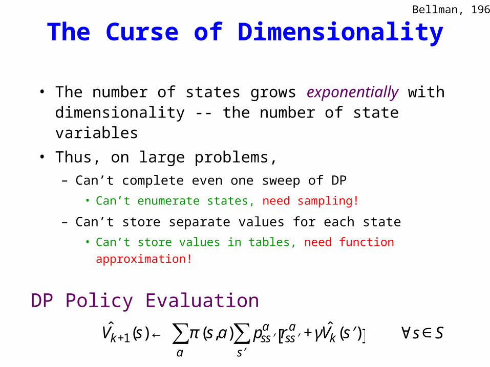
• The number of states grows exponentially with dimensionality -- the number of state variables

• Thus, on large problems,– Can’t complete even one sweep of DP

• Can’t enumerate states, need sampling!

– Can’t store separate values for each state

• Can’t store values in tables, need function approximation!

DP Policy Evaluation

Bellman, 1961

ˆ V k1 (s) (s,a)a

ps s a rs s

a ˆ V k ( s ) s

s S

ˆ V k1(s) d(s) (s,a)a

ps s a rs s

a ˆ V k ( s ) s


Some distribution over states, possibly uniform

s S

These terms can bereplaced by sampling

ˆ V k1 (s) (s,a)a

ps s a rs s

a ˆ V k ( s ) s

s S


ps s a rs s

a ˆ V k ( s ) s


s S

For each sample transition, s,a s’,r :

ˆ V (s)← ˆ V (s)+α r +γˆ V ( ′ s )− ˆ V (s)[ ]

Sutton, 1988; Witten, 1974Tabular TD(0)

lim ˆ V (s)=Vπ (π)

Sampling vs Enumeration

ˆ V k1 (s) (s,a)a

ps s a rs s

a ˆ V k ( s ) s

s S


ps s a rs s

a ˆ V k ( s ) s


s S

Sample Returns can also be either

r r 2 r L

r

r

r

r ˆ V ( s )

As in the general TD(λ) algorithm

Full or Truncated

Function Approximation

• Store values as a parameterized form

• Update , e.g., by gradient descent: ̂ V (s)= f(s,

r θ )

cf. DP Policy Evaluation (rewritten to include a step-size ):

ˆ V k+1(s)← ˆ V k(s)+α d(s) π(s,a)a∑ ps ′ s

a rs ′ s a +γˆ V k( ′ s )− ˆ V k(s)[ ] ∀s∈S

′ s ∑

r θ k+1 =

r θ k +α d(s)

s∑ π(s,a)

a∑ ps ′ s

a rs ′ s a +γˆ V k( ′ s )− ˆ V k(s)[ ]

′ s ∑ ∇ r

θ ˆ V k(s)

Linear Function Approximation

ˆ V (s)=

r θ T

r φ s ∇

r θ

ˆ V (s)=r φ s

Each state s represented by a feature vector

Or respresent a state-action pair withand approximate action values:

r φ s

Qπ (s,a)=Eπ Rt st =s,at =a

ˆ Q (s,a)=

r θ T

r φ s,a

r φ sa

Linear TD(λ)

After each episode:

where

θ ← θ + Δθtt=0

T−1

∑

Δθt =α Rtλ −θTφstat[ ]φstat

Rtλ =(1−λ) λn−1Rt

(n)

n=1

∞

∑

Rt(n) =rt+1+γ rt+2 +L +γn−1rt+n +γnθTφst+nat+n

“n-step return”

rt1 Tst1at1

“λ-return”

e.g.,

Sutton, 1988

RoboCup

• Use soccer as a rich and realistic testbed• Robotic and simulation leagues

– Open source simulator (Noda)

An international AI and Robotics research initiative

Research Challenges• Multiple teammates with a common goal• Multiple adversaries – not known in advance• Real-time decision making necessary• Noisy sensors and actuators• Enormous state space, > 2310 states

9

RoboCup Feature Vectors

.

.Sparse, coarse,

tile codingLinearmap

.

.

.

.

.

.

.

.

.Full

soccerstate

actionvalues

Huge binary feature vector(about 400 1’s and 40,000 0’s)

13 continuousstate variables

r s

13 Continuous State Variables(for 3 vs 2)

11 distances amongthe players, ball,and the center ofthe field

2 angles to takersalong passing lanes

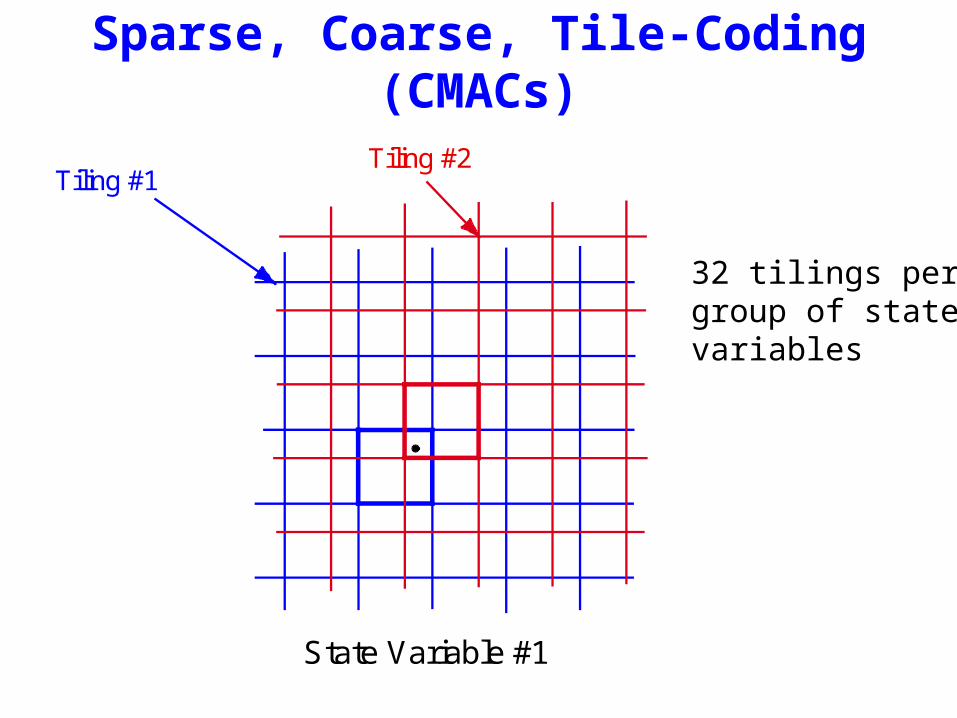
Sparse, Coarse, Tile-Coding (CMACs)

Tiling #1Tiling #2

State Variable #1

State Variable #2

32 tilings pergroup of statevariables

Learning Keepaway Results3v2 handcrafted takers

0 10 20 254

6

8

10

12

14

EpisodeDuration(seconds)

Hours of Training Time(bins of 1000 episodes)

handcoded randomalwayshold

Multiple,independentruns of TD(λ)

Stone & Sutton, 2001

Key Distinctions






– The distribution d(s)

Off-Policy Instability

• Examples of diverging k are known for– Linear FA– Bootstrapping

• Even for– Prediction– Enumeration– Uniform d(s)

• In particular, linear Q-learning can diverge

Baird, 1995

Gordon, 1995

Bertsekas & Tsitsiklis, 1996

Baird’s Counterexample

0 + 2θ1

ε1 − ε

θ0 + 2θ2 θ0 + 2θ3 θ0 + 2θ4 θ0 + 2θ5

2θ0 + θ6

0

5

10

0 1000 2000 3000 4000 5000

10

10

/ -10

Iterations (k)

510

1010

010

-

-

Parametervalues, k(i)

(logscale,brokenat

Markov chain (no actions)

All states updated equally often, synchronously

Exact solution exists: = 0

Initial 0 = (1,1,1,1,1,10,1)T

100%

±1)

On-Policy Stability

• If d(s) is the stationary distribution of the MDP under policy (the on-policy distribution)

• Then convergence is guaranteed for– Linear FA– Bootstrapping– Sampling– Prediction

• Furthermore, asymptotic mean square error is a bounded expansion of the minimal MSE:

Tsitsiklis & Van Roy, 1997

Tadic, 2000

MSE(θ∞)=1−γλ1−γ

minθ

MSE(θ)

— Value Function Space —

inadmiss

able value fu

nctions

value fu

nctions c

onsiste

nt with

param

eteriz

ation

True V*Region of *

best admissable

policy

Original naïve hope

guaranteed convergenc

eto good

policy

Res gradient et al.

guaranteed convergenc

eto less

desirable policy

Sarsa, TD(λ) & other on-policy methods

chatteringwithout

divergence or guaranteed

convergence

Q-learning, DP & otheroff-policy methods

divergence possible

V*best

admissablevalue fn.

There are Two Different Problems:

Chattering• Is due to Control + FA

• Bootstrapping not involved

• Not necessarily a problem

• Being addressed with policy-based methods

• Argmax-ing is to blame

Instability• Is due to Bootstrapping + FA + Off-Policy

• Control not involved

• Off-policy is to blame

Yet we need Off-policy Learning

• Off-policy learning is needed in all the frameworks that have been proposed to raise reinforcement learning to a higher level– Macro-actions, options, HAMs, MAXQ– Temporal abstraction, hierarchy, modularity– Subgoals, goal-and-action-oriented perception

• The key idea is: We can only follow one policy,but we would like to learn about many policies,in parallel– To do this requires off-policy learning

On-Policy Policy Evaluation Problem

Use data (episodes) generated by to learn

ˆ Q ≈Qπ

Off-Policy Policy Evaluation Problem

Use data (episodes) generated by ’ to learn

ˆ Q ≈Qπ

behavior policy Targetpolicy


Naïve Importance-Sampled TD(λ)

1 2 3 L T-1

ρt =π(st,at)′ π (st,at)

importance samplingcorrection ratio for t

Relative prob.of episode under and ’

We expect this to have relatively high variance


Per-Decision Importance-Sampled TD(λ)

1 2 3 L t

ρt =π(st,at)′ π (st,at)

R tλis like , except in terms ofRt

λ

R t(n) =rt+1 +γ rt+2 ρt+1+γ rt+2 ρt+1ρt+2 +L

+γnρt+1L ρt+nθTφst+nat+n

Per-Decision TheoremPrecup, Sutton & Singh (2000)

E ′ π R tλ st,at =Eπ Rt

λ st,at

New Result for Linear PD Algorithm

Precup, Sutton & Dasgupta (2001)

E ′ π Δθ s0,a0 =Eπ Δθ s0,a0

Total change over episode for new algorithm

Total change forconventional TD(λ)

Convergence Theorem• Under natural assumptions

– S and A are finite– All s,a are visited under ’– and ’ are proper (terminate w.p.1)– bounded rewards

– usual stochastic approximation conditions on the step size k

• And one annoying assumption

• Then the off-policy linear PD algorithm converges to the same as on-

policy TD(λ)

var ′ π ρ1ρ2L ρT−1[ ]<B<∞ ∀s1 ∈S

e.g., bounded episode length

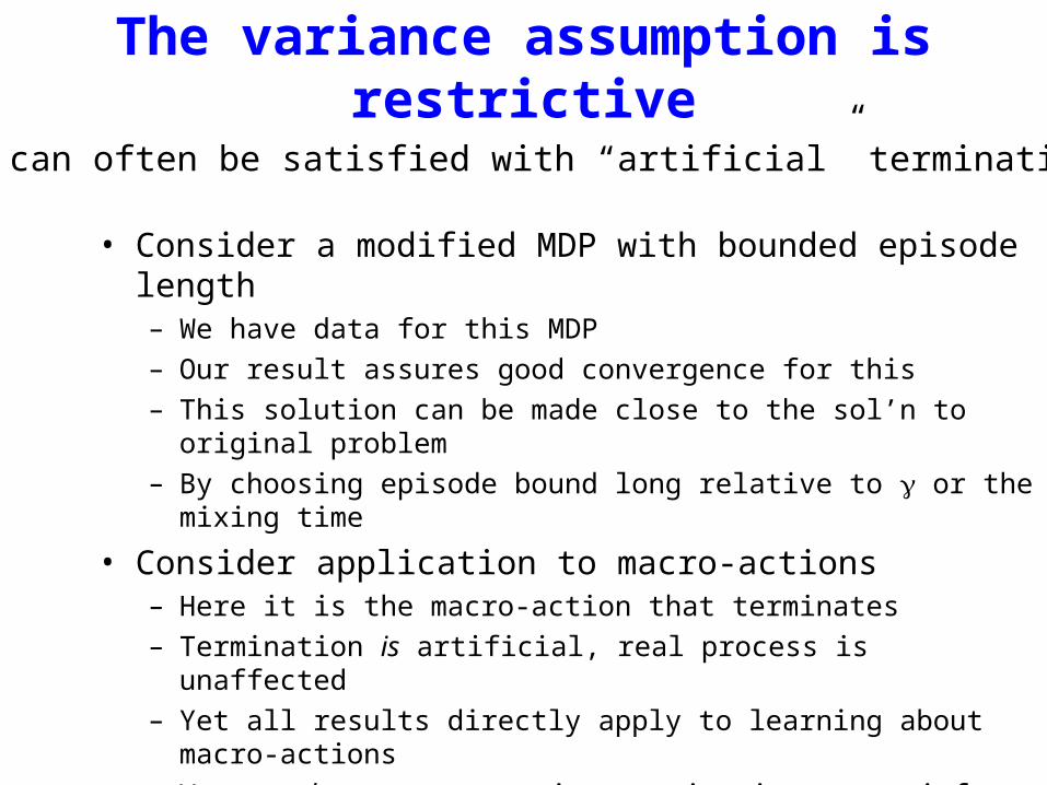
The variance assumption is restrictive

• Consider a modified MDP with bounded episode length– We have data for this MDP– Our result assures good convergence for this– This solution can be made close to the sol’n to original

problem– By choosing episode bound long relative to or the

mixing time

• Consider application to macro-actions– Here it is the macro-action that terminates– Termination is artificial, real process is unaffected– Yet all results directly apply to learning about macro-

actions– We can choose macro-action termination to satisfy the

variance condition

But can often be satisfied with “artificial” terminations

Empirical Illustration

Agent always starts at STerminal states marked GDeterministic actions

Behavior policy choosesup-down with 0.4-0.1 prob.

Target policy choosesup-down with 0.1-0.4

If the algorithm is successful, it should give positiveweight to rightmost feature, negative to the leftmost one

Trajectories of Two Components of

λ = 0.9 decreased

appears to converge as advertised

-0.4

-0.3

-0.2

-0.1

0

0.1

0.2

0.3

0.4

0.5

0 1 2 3 4 5

Episodes x 100,000

µlef tmost ,down

µlef tmost ,down

µr ightmost ,down

*

µr ightmost ,down*

Comparison of Naïve and PD IS Algs

1

1.5

2

-12 -13 -14 -15 -16 -17

2.5

RootMean

SquaredError

Naive IS

Per-Decision IS

Log2

λ = 0.9 constant

(after 100,000episodes, averaged

over 50 runs)

Precup, Sutton & Dasgupta, 2001

Can Weighted IS help the variance?

Return to the tabular case, consider two estimators:

QnIS(s,a)=1

n Riwii=1

n

∑ith return following s,a

IS correction product

t1 t2 t3 L T 1(s,a occurs at t )

converges with finite variance iff the wi have finite variance

QnISW(s,a)=

Riwii=1

n

∑

wii=1

n

∑

converges with finite variance even if the wi have infinite variance

Can this be extendedto the FA case?

Restarting within an Episode

• We can consider episodes to start at any time

• This alters the weighting of states,– But we still converge,– And to near the best answer (for the new weighting)

Incremental Implementation

At the start of each episode:

c0 =g0r e 0 =c0φ0

On each step: st at → rt+1 st+1 at+1 0<t<T

ρt+1 =π(st+1,at+1) ′ π (st+1,at+1)

δt =rt+1 +γ ρt+1θTφt+1−θTφt

Δθt =αδtr e t

ct+1 =ρt+1ct +gt+1r e t+1 =γ λ ρt+1

r e t +ct+1φt+1

Key Distinctions






Harder,more challengingand interesting

Easier,conceptually

simpler

Conclusions

• RL is beating the Curse of Dimensionality– FA and Sampling

• There is a broad frontier, with many open questions

• MDPs: States, Decisions, Goals, and Probability is a rich area for mathematics and experimentation

Documents

Overcoming the Curse of Dimensionality with Reinforcement Learning Rich Sutton AT&T Labs with thanks to Doina Precup, Peter Stone, Satinder Singh, David