Embed Size (px)
Citation preview
TRACTABLE MEASURE OF COMPONENT OVERLAPFOR GAUSSIAN MIXTURE MODELS
EWA NOWAKOWSKA, JACEK KORONACKI, AND STAN LIPOVETSKY
Abstract. The ability to quantify distinctness of a cluster structure is fun-damental for certain simulation studies, in particular for those comparing per-formance of different classification algorithms. The intrinsic integral measurebased on the overlap of corresponding mixture components is often analyt-ically intractable. This is also the case for Gaussian mixture models withunequal covariance matrices when space dimension d > 1. In this work wefocus on Gaussian mixture models and at the sample level we assume the classassignments to be known. We derive a measure of component overlap basedon eigenvalues of a generalized eigenproblem that represents Fisher’s discrim-inant task. We explain rationale behind it and present simulation results thatshow how well it can reflect the behavior of the integral measure in its lin-ear approximation. The analyzed coefficient possesses the advantage of beinganalytically tractable and numerically computable even in complex setups.
1. Introduction
1.1. Overview. There are numerous measures designed to capture distance be-tween distributions or – more specifically – overlap between components of a Gauss-ian mixture model. One of the oldest is the Bhattacharyya coefficient (see forinstance [1] or [2]), which reflects the amount of overlap between two statisticalsamples or distributions, a generalization of Mahalanobis distance described in [3]or [4]. In the context of information theory the most generic is the Kullback-Leiblerdivergence (see [5]) – a non-symmetric measure of difference between two distribu-tions, also interpreted as expected discrimination information, which sets the linkwith possible classification performance. In [6] an overlap coefficient is proposedthat measures agreement between two distributions, it is applied to samples of datacoming from normal distributions. Among more recent works, in [7] a c-separationmeasure between multidimensional Gaussian distributions is defined, later devel-oped in [8] as exact-c-separation. In [9], in the setup simplified to two clusters k = 2and two dimensions d = 2, overlap rate is defined as a ratio of the joint densityin its saddle point to its lower peak. The concept of ridge curve is introduced andfurther developed in [10] and [11], generalized to arbitrary number of dimensionsand clusters, turning the ridge curve into a ridgeline manifold of the dimensionk − 1.
All the measures use the parameters of the distributions to assess the overlapbetween the components and are typically formulated in terms of the underlyingmodel. However, they can also be applied at the data level, as long as the class
2000 Mathematics Subject Classification. 62H30, 62E99.Key words and phrases. mixture model, cluster structure, overlap measure.Supported by National Science Center of Poland, DEC-2011/01/N/ST6/04174.
1
arX
iv:1
407.
7172
v1 [
mat
h.ST
] 2
7 Ju
l 201
4

2 EWA NOWAKOWSKA, JACEK KORONACKI, AND STAN LIPOVETSKY
(or cluster) assignment is known. Then the model parameter estimates are usedinstead instead.
1.2. Content. In Section 2 we recall the generic concept of component overlap andits best linear approximation, we also show an example of an overlap assessmentapproach and point to common difficulties. Then, in Section 3 we introduce whatwe refer to as Fisher’s distinctness measure and we explain rationale behind it.Finally, in Section 4 we show results of a simulation study that illustrates howwell the Fisher’s coefficient can reflect the linear approximation of the originalintractable overlap coefficient.
2. Overlap of Distributions
2.1. Integral measure. The most generic and natural coefficient of overlap be-tween components is what follows directly from the mixture definition:
MLEerr = 1−∫Rd
max(π1f1(µ1,Σ1), . . . , πkfk(µk,Σk)
)(x)dx,
which for k = 2 classes simplifies to
(1) MLEerr =
∫Rd
min(π1f1(µ1,Σ1), π2f2(µ2,Σ2)
)(x)dx,
where for d ≥ 1 by fi, i = 1, . . . , k we denote component densities and by πi,i = 1, . . . , k their corresponding mixing factors. Throughout this work we willassume though that equal mixing factors are assigned to all the components, whichcorresponds to balanced cluster sizes at the sample level. Coefficient (1) measuresthe actual overlap between two probability distribution and for d = 1 is illustratedin Figure 1. It coincides with intuitive understanding of components’ overlap andwith its expected behavior — grows with increasing within cluster dispersion (orvariance, for d = 1) and decreasing distance between cluster centers. Also, itexhibits a strong link with classification performance, setting the upper limit forpossible predictive accuracy in terms of maximum likelihood estimation (MLE) (seefor instance [12]). Namely, best classification procedures based on likelihood ratio(MLE) or — equivalently — on its logarithm are given by
(2) loglik(f1, f2)(x) = log(f2(µ2,Σ2)(x)
f1(µ1,Σ1)(x)
).
Figure 1. Overlap (dark shadow) betweenk = 2 Gaussian components in d = 1 dimen-sion, concept illustration.
For the value of (2) less than a con-stant observation x is classified to thefirst cluster, to the second otherwise.Hence the area of overlap betweenthe components, as given by 1, cor-responds to the expected proportionof observations that are incorrectlyclassified by MLE-classification rule,based on the (estimated) parametersof the mixture. Therefore (1) is de-noted by MLEerr and alternativelyreferred to as MLE-misclassificationor error rate.

OVERLAP MEASURE FOR GAUSSIAN MIXTURE MODELS 3
The fundamental problem with formula (1), and also one of the reasons for nu-merous alternative approaches to overlap assessment, is that (1) is hardly tractablefor mixtures with different covariance matrices in higher dimensions. Handling itanalytically would require integrating functions of Gaussian density over regionswhose description often does not possess a tractable formulaic description either.Therefore, it can only be treated as a theoretical overlap coefficient for Gaussianmixture models and for practical applications replaced with other approaches.
2.2. Best linear approximation. The authors of [13] propose an approximationof (1) — best linear separator for k = 2 Gaussian components in d ≥ 1 dimensionsand an algorithm to determine it for a given data set X. They derive a linearfunction of x ∈ Rd given by a vector b ∈ Rd such that for a given constant c ∈ Rinequality bTx ≤ c classifies observation x to the first cluster, while bTx > c tothe second. Vector b and constant c are obtained iteratively in order to minimizemaximal probability of misclassification. As this approach will be used in oursimulations, it is described below in more details following [13].
For x coming from component l = 1, 2, bTx has a univariate normal distributionwith mean bTµl and variance bTΣlb. As such, the probability of misclassifyingobservation x when it comes from the first population l = 1 equals(3)
P1
(bTx > c
)= P1
(bTx− bTµ1
bTΣ1b>c− bTµ1
bTΣ1b
)= 1− Φ
(c− bTµ1
bTΣ1b
)= 1− Φ
(u1),
where Φ denotes cumulative distribution function for a univariate standardizednormal distribution (centered at zero, with variance equal to one) and u1 = c−bTµ1
bTΣ1b.
Similarly, probability of misclassifying observation x when it comes from the secondpopulation l = 2 equals
(4) P2
(bTx ≤ c
)= P1
(bTx− bTµ2
bTΣ2b≤ c− bTµ2
bTΣ2b
)=
= Φ
(c− bTµ2
bTΣ2b
)= 1− Φ
(bTµ2 − cbTΣ2b
)= 1− Φ (u2) ,
for u2 = bTµ2−cbTΣ2b
. As Φ is monotonic, the task
max(P1(u1),P2(u2)
)−→ min
b∈Rd
c∈R
is equivalent to
(5) min(u1, u2) −→ maxb∈Rd
c∈R
,
which is more convenient to work with. As the objective is to find b ∈ Rd andc ∈ R that minimize maximal probability of misclassification, we will refer to theresulting procedure as a minimax procedure. Analytical formulation of admissibleprocedures for b and c leads to the following characterization
(6) b = (t1Σ1 + t2Σ2)−1
(µ2 − µ1)
and
(7) c = bTµ1 + t1bTΣ1b = bTµ2 − t2bTΣ2b,

4 EWA NOWAKOWSKA, JACEK KORONACKI, AND STAN LIPOVETSKY
where t1 ∈ R and t2 ∈ R are scalars. Minimax procedure is an admissible procedurewith u1 = u2. As such, for t = t1 = (1− t2) the following equality must hold
(8) 0 = u21 − u22 = t2bTΣ1b− (1− t)2bTΣ2b = bT[t2Σ1 − (1− t)2Σ2
]b.
Equation (8) for t can be solved numerically by means of iterative procedure.With the above derivations, for a mixture of k = 2 components in d ≥ 1 di-
mensions with parameters µ1,Σ1 and µ2,Σ2 respectively, the following algorithmprovides best linear separator in terms of minimizing the maximal probability ofmisclassification.
Algorithm 2.1: BestLinearSeparator(µ1,Σ1, µ2,Σ2, prec)
initialize incr, crit, trepeatcalculate b with (6)calculate crit with (8)if crit > precthen t← t− incr
if crit < −precthen t← t+ incr
incr ← incr · 12until criterion crit given by (8) met with expected precision preccalculate c with (7)calculate u1 and u2 and the probabilities of misclassification with (3) and (4)calculate overall probability of misclassification Pminmax = max(P1(u1),P2(u2))return (Pminmax, b, c, t)
Note that the value of assumed precision prec must be given, while the valuesof scalar t, criterion crit and increment incr must be initialized. What is more,Pminmax = P1(u1) = P2(u2)) as for the minimax procedure u1 = u2 must hold.Note, that Pminmax may be considered a measure of overlap as a result of linearapproximation of criterion (2). If Σ1 = Σ2, formula (2) and its linear approximationgiven by b and c coincide, which is sure not the case for Σ1 6= Σ2.
2.3. The challenge of replacement. Degree of overlap between mixture compo-nents is critical for classification performance and must be assessed for simulationpurposes and comparison of classification methods, hence the interest in the topic.There are many measures proposed in the literature that possess the property ofbeing tractable even in a complex setup, however it is highly required that theirbehavior reflects the behavior of MLEerr based either on (1) or on its linear approx-imation of the previous subsection. However, this is not always the case, as shownin the below example.
E-distance. The method for overlap assessment proposed in [14] does not as-sume underling normal mixture model, however it can be very well applied in suchsetup. It is considered an extension to Ward’s minimum variance method (see[15]) that formally takes both into account — heterogeneity between groups andhomogeneity within groups in data. For this purpose it uses joint between-withine-distance between clusters that constitutes the basis for agglomerative hierarchi-cal clustering procedure the authors propose. They define e-distance between two

OVERLAP MEASURE FOR GAUSSIAN MIXTURE MODELS 5
sets of observations X1 = {xi1 : c(i1) = 1}, n1 = |X1| and X2 = {xi2 : c(i2) = 2},n2 = |X2| as
(9) e(X1, X2) =n1n2n1 + n2
2
n1n2
∑i1 : c(i1)=1
∑i2 : c(i2)=2
‖xi1 − xi2‖ +
− 1
n21
∑i1 : c(i1)=1
∑j1 : c(j1)=1
‖xi1 − xj1‖ −1
n22
∑i2 : c(i2)=2
∑j2 : c(j2)=2
‖xi2 − xj2‖
.
The value of e-distance between two resulting clusters may be considered a clusterstructure distinctness measure. It is expected to reflect changes in within-clusterdispersion and between-cluster separation. It should also remain in tune with thetheoretical structure distinctness measure given by likelihood ratio (2) or its linearapproximation from [13].
0.75
0.80
0.85
0.90
0.95
1.00
1.0 1.5 2.0 2.5 3.0
1.0
1.5
2.0
2.5
3.0
Clusterability ! heat map
between!cluster distance
with
in!
clu
ste
r d
isp
ers
ion
Figure 2. Heatmap —Anderson-Bahadur mis-classification error w/rto growing between (x-axis) and within (y-axis) cluster dispersion.
1000
1500
2000
2500
1.0 1.5 2.0 2.5 3.0
1.0
1.5
2.0
2.5
3.0
Szekely!Rizzo e!distance ! heat map
between!cluster distance
with
in!
clu
ste
r d
isp
ers
ion
Figure 3. Heatmap— Székely-Rizzo e-distance (9) w/rto growing between(x-axis) and within (y-axis) cluster dispersion.
Figures 2 and 3 compare variability of structure distinctness measures based onAnderson-Bahadur ([13]) and Székely-Rizzo ([14]) proposals respectively. The for-mer, similarly to the likelihood ratio theoretical distinctness measure, does dependon both — between-cluster distance and within-cluster dispersion, while the lat-ter essentially remains insensitive to within cluster dispersion, depending entirelyon the between class separation. This is an empirical insight which shows substan-tial discrepancy between behavior of theoretical and intuitive structure distinctnessmeasure and e-distance given by (9), and hence points to another potential difficultywhen trying to replace the integral coefficient.
6 EWA NOWAKOWSKA, JACEK KORONACKI, AND STAN LIPOVETSKY
3. Fisher’s distinctness measure
3.1. Model and notation. We consider a data set X = (x1, . . . , xn)T , X ∈ Rn×dof n observations coming from a mixture of k d-dimensional normal distributions
f(x) = π1f1(µ1,Σ1)(x) + . . .+ πkfk(µk,Σk)(x),
wherefl(µl,Σl)(x) =
1
(√
2π)d√
det Σl
e−12 (x−µl)
TΣ−1l (x−µl).
We call each fl(µl,Σl), l = 1, . . . , k a component of the mixture and each πl,l = 1, . . . , k a mixing factor of the corresponding component (see [12] or [16] and[17] or [18] for comparison with alternative approaches). We assume that for allthe components equal mixing factors are assigned π1 = · · · = πk = 1
k . However,we allow different covariance matrices Σl. Additionally, we assume large spacedimension with respect to the number of components d > k − 1 and take thenumber of components k and class assignments as known.
We use lower index to indicate data set when sample estimates of parametersare used. In particular, by µX ∈ Rd we denote sample mean and by ΣX ∈ Rd×dcovariance matrix for a data set X. For notation ease we center the data at theorigin µX = 0. We assume the covariance matrix to be of full rank, rank(ΣX) = d.Let TX = nΣX be the total scatter matrix forX. We recall that a simple calculation(see for instance [12] or [19]) splits total scatter into its between and within clustercomponents TX = BX + WX . By µX,l and ΣX,l we denote empirical mean andcovariance matrix for class l, where l = 1, . . . , k. By MX = (µX,1, . . . , µX,k),MX ∈ Rd×k we understand a matrix of column vectors of cluster means. Weassume the cluster means — as a set of points — to be linearly independent, sorank(MX) = min(d, k − 1) = k − 1.
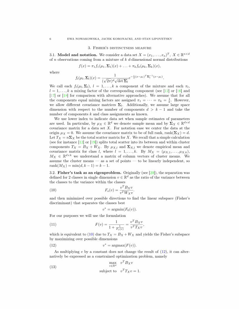
3.2. Fisher’s task as an eigenproblem. Originally (see [20]), the separation wasdefined for 2 classes in single dimension v ∈ Rd as the ratio of the variance betweenthe classes to the variance within the classes
(10) Fo(v) =vTBXv
vTWXv.
and then minimized over possible directions to find the linear subspace (Fisher’sdiscriminant) that separates the classes best
v∗ = argmin(F0(v)).
For our purposes we will use the formulation
(11) F (v) =1
1 + 1Fo(v)
=vTBXv
vTTXv,
which is equivalent to (10) due to TX = BX +WX and yields the Fisher’s subspaceby maximizing over possible dimensions
(12) v∗ = argmax(F (v)).
As multiplying v by a constant does not change the result of (12), it can alter-natively be expressed as a constrained optimization problem, namely
(13)maxv∈Rd
vTBXv
subject to vTTXv = 1.

OVERLAP MEASURE FOR GAUSSIAN MIXTURE MODELS 7
The corresponding Lagrange function defined as
L(v;λ) = vTBXv + λ(vTTXv − 1
)yields
∂L(v;λ)
∂v= 2BXv − 2λTXv = 0,
so
(14) BXv = λTXv
must hold at the solution. Problem (14) is a generalized eigenproblem for twomatrices BX and TX . As we assume covariance matrix to be well-defined, totalscatter matrix TX is invertible, however T−1X BX is not necessarily symmetric soit is a priori not obvious if the eigenvalues are real. Hence, a decomposition ofthe matrix TX is required to reduce the generalized eigenproblem to a standardeigenproblem for a transformed matrix.
Solving a standard eigenproblem for TX we obtain
(15) TX = ATXLTX
ATTX.
Note, that ATXis orthonormal (i.e. ATX
ATTX= I so A−1TX
= ATTX). Replacing in
(14) matrix TX with its spectral decomposition (15) we get
BXv = λATXLTX
ATTXv = λATX
L1/2TXL1/2TXATTX
v,
then multiplying by (ATXL1/2TX
)−1 from the left and by I in the middle we transformit to
L−1/2TX
ATTXBXATX
L−1/2TX
L1/2TXATTX
v = λL1/2TXATTX
v.
Now, substituting
B = L−1/2TX
ATTXBXATX
L−1/2TX
=(L−1/2TX
ATTX
)BX
(L−1/2TX
ATTX
)Tand
(16) v = L1/2TXATTX
v
we get a standard eigenproblem for B
(17) Bv = λv.
Solving (17) and using the inverse transformation of (16)
(18) v = ATXL−1/2TX
v,
we obtain the solution v to the original problem (14), corresponding to the sameeigenvalue λ. In particular, it proves that with our model assumptions (14) can bereduced to a standard eigenproblem
(19) T−1X BXv = λv,
which takes the matrix form of
(20)(T−1X BX
)V = V L,
where L ∈ Rd×d is a diagonal matrix of eigenvalues in a non-decreasing order andV ∈ Rd×d is a matrix of their corresponding column eigenvectors.
Note that there is another alternative formulation of the problem (14) via canon-ical correlation analysis (CCA), which may also come as a convenient way to see

8 EWA NOWAKOWSKA, JACEK KORONACKI, AND STAN LIPOVETSKY
the task. In this setup Fisher’s eigenvalues correspond to squared canonical cor-relation coefficients. We will not describe it here in details but we give referencesfor interested readers. The approach, referred to as canonical discriminant analysis(CDA), was first mentioned in [21] and thoroughly described in [22]. The overviewof classical CCA is given for instance in [12].
3.3. Motivation. What we refer to as Fisher’s distinctness measure was inspiredby [23], where the idea of using the eigenproblem formulation of the Fisher’s dis-crimination task and its respective eigenvalues for assessing certain properties ofdata was used.
As explained in Subsection 3.2, Fisher’s discriminant task can be stated in termsof eigenproblem given by (20). Then, its (k − 1) eigenvectors corresponding tothe (k − 1) non-zero eigenvalues span the Fisher’s subspace. Note that there arek − 1 non-zero eigenvalues as according to the model assumptions rank(TX) = dand rank(BX) = k − 1 and d > k − 1. Due to (20) we have
V TT−1X BXV = L,
so the eigenvalues capture variability in the spanning directions. As Fisher’s taskis scale invariant, the increase in variability may only be due to increase in betweencluster scatter or decrease in within cluster scatter so it is expected to captureincrease in structure distinctness very well. As squared canonical correlation coef-ficients (see references in Subsection 3.2), the eigenvalues remain in the interval of[0, 1] which also makes them easy to compare and interpret. Additionally, exceptfor being easy to compute numerically, they are also convenient to handle analyt-ically, so they can easily be used in simulations as well as formal derivations andjustifications. What remains, is to propose function of the eigenvalues that couldserve as structure distinctness coefficient and analyze its performance. This wasdone by means of simulation study and described in the next section.
4. Simulation study
4.1. Overview. Due to its analytical complexity (1) is virtually intractable formixtures with varied covariance matrices (heterogeneous) or of higher space di-mension. However, it relatively easy undergoes simulations of Monte Carlo kindand can easily be approximated numerically with the best linear approximationdescribed in subsection 2.2. As such, it may be used as a reference measure andreplaced with another coefficient that reflects its behavior but offers the advantageof being computable and analytically tractable, also in a more complex setup.
The study was divided into two parts. In the first part two dimensional case wasstudied in details. Normal distribution was parametrized in a way that allowed foreasy parameter control. Then all the possible combinations were tested and theinfluence of change in between cluster separation and within cluster dispersion wasanalysed. Three possible structure distinctness measures were compared — exactintegral measure (1), its best linear approximation described in subsection 2.2 andFisher’s eigenvalue. For two dimensional data, the maximum number of two clusterswas analysed (due to the assumption of d > k − 1), which led to one dimensionalprojections. Therefore, there was just single Fisher’s eigenvalue to compare sothe two dimensional step could not give grounds for function selection. The twodimensional study served as a thorough assessment of single Fisher’s eigenvalueperformance.

OVERLAP MEASURE FOR GAUSSIAN MIXTURE MODELS 9
In the second step multidimensional data was analyzed. Due to high number ofpossible mixture parameter combinations only a random selection was considered.This step was meant to confirm satisfactory performance of Fisher eigenvalues asinput for structure distinctness measure. Higher dimensionality allowed for largernumber of clusters, which resulted in (k−1) > 1 dimensionality of Fisher’s subspace.As such, it also gave grounds for selecting appropriate function to transform (k −1) eigenvalues into a single structure distinctness coefficient. Minimum λXmin andaverage λX over Fisher’s non-zero eigenvalues were calculated as follows
(21) λXmin = minj∈{1,...,k−1}
λT−1X BX
j
and
(22) λX =1
k − 1
k−1∑j=1
λT−1X BX
j ,
and compared with the Monte Carlo estimates of the integral measure (1). Notethat due to the larger number of classes allowed, wider comparisons with the bestlinear separator, defined for k = 2 only, were infeasible.
Note that although the original concept (1) is defined in terms of overlap (simi-larity) between the components, what is naturally captured by either minimum oraverage over non-zero Fisher’s eigenvalues, reflects the opposite behavior, so shouldrather be referred to as distinctness (dissimilarity) measure. Therefore we compareit with (1 −MLEerr) (or (1 − Pminmax)), which is the probability of correct MLEclassification (or its best linear approximation). The transition from one to anotheris typically straightforward, however we point that out explicitly to avoid confusionor additional transformations of the coefficients.
Algorithm 4.1: TwoDimensionalDataGeneration(r, α, λ, q, k,N [])
for each cluster l ∈ {1, . . . , k}
do
comment:Determine cluster center µ
µ←(r · sin
((l − 1) · 2πk
), r · cos
((l − 1) · 2πk
))comment:Compute covariance matrix Σ
D ← diag(λ, q · λ) comment: dispersion and shape matrix
R←(
cos(α) − sin(α)sin(α) cos(α)
)comment: rotation matrix
Σ← RDRT
comment:Generate data
draw N [l] observationsadd cluster mean µ to each observation
return (data)
4.2. Two-dimensional simulations. To allow for easy control over mixture pa-rameters, two dimensional mixture density was parametrized in a convenient way.Cluster centers were located on a circle around origin (0, 0) with radius r that
10 EWA NOWAKOWSKA, JACEK KORONACKI, AND STAN LIPOVETSKY
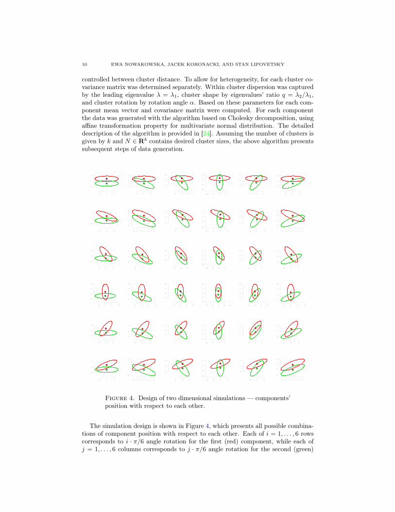
controlled between cluster distance. To allow for heterogeneity, for each cluster co-variance matrix was determined separately. Within cluster dispersion was capturedby the leading eigenvalue λ = λ1, cluster shape by eigenvalues’ ratio q = λ2/λ1,and cluster rotation by rotation angle α. Based on these parameters for each com-ponent mean vector and covariance matrix were computed. For each componentthe data was generated with the algorithm based on Cholesky decomposition, usingaffine transformation property for multivariate normal distribution. The detaileddescription of the algorithm is provided in [24]. Assuming the number of clusters isgiven by k and N ∈ Rk contains desired cluster sizes, the above algorithm presentssubsequent steps of data generation.
−5 0 5
−5
05
−5 0 5
−5
05
−5 0 5
−5
05
−5 0 5 10
−5
05
10
−5 0 5
−5
05
−5 0 5
−5
05
−5 0 5
−5
05
−6 −4 −2 0 2 4 6
−6
−2
24
6
−5 0 5
−5
05
−5 0 5 10
−5
05
10
−5 0 5
−5
05
−6 −4 −2 0 2 4 6
−6
−2
24
6
−5 0 5
−5
05
−5 0 5
−5
05
−5 0 5
−5
05
−5 0 5 10
−5
05
10
−5 0 5
−5
05
−5 0 5
−5
05
−10 −5 0 5
−10
−5
05
−10 −5 0 5
−10
−5
05
−10 −5 0 5
−10
−5
05
−10 −5 0 5 10
−10
−5
05
10
−10 −5 0 5
−10
−5
05
−10 −5 0 5
−10
−5
05
−5 0 5
−5
05
−5 0 5
−5
05
−5 0 5
−5
05
−5 0 5 10
−5
05
10
−5 0 5
−5
05
−5 0 5
−5
05
−5 0 5
−5
05
−6 −4 −2 0 2 4 6
−6
−2
24
6
−5 0 5
−5
05
−5 0 5 10
−5
05
10
−5 0 5
−5
05
−6 −4 −2 0 2 4 6
−6
−2
24
6
Figure 4. Design of two dimensional simulations — components’position with respect to each other.
The simulation design is shown in Figure 4, which presents all possible combina-tions of component position with respect to each other. Each of i = 1, . . . , 6 rowscorresponds to i · π/6 angle rotation for the first (red) component, while each ofj = 1, . . . , 6 columns corresponds to j · π/6 angle rotation for the second (green)
OVERLAP MEASURE FOR GAUSSIAN MIXTURE MODELS 11
component. Altogether it yields 36 basic mixture positions. For each position aninfluence of a single factor is analyzed and this includes in particular – increase inbetween cluster distance (Figures 7 and 8), increase in within cluster dispersion forboth (Figures 9 and 10) and for first (Figures 11 and 12) and second (Figures 13and 14) spanning direction only. The special case of spherical clusters is analyzedseparately (Figures 15 to 18). All the results are available in Appendix, Section A.
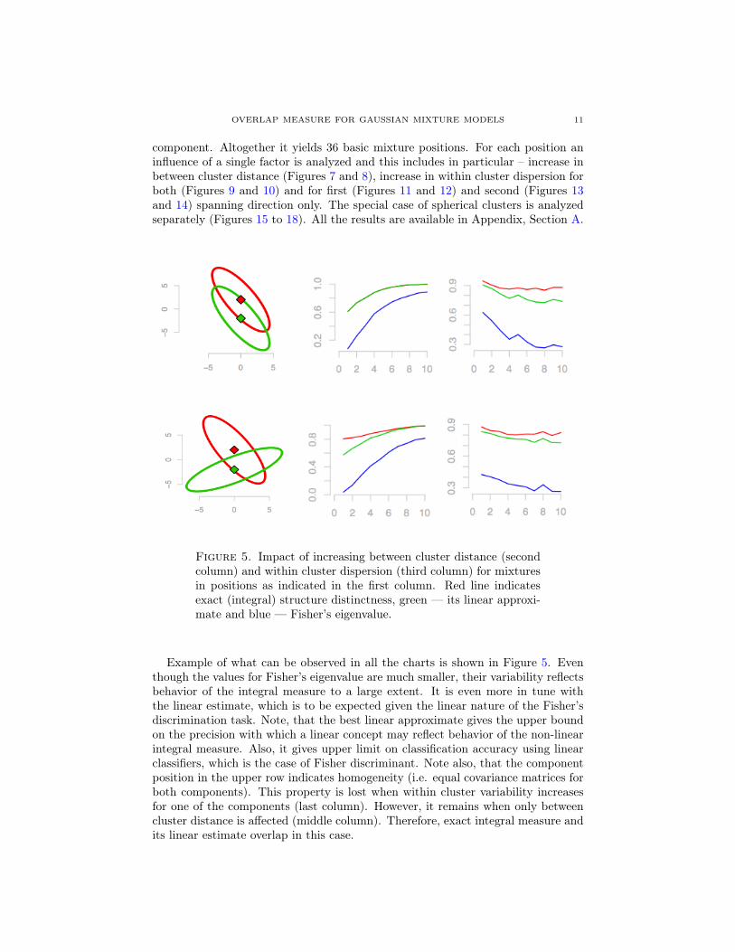
Figure 5. Impact of increasing between cluster distance (secondcolumn) and within cluster dispersion (third column) for mixturesin positions as indicated in the first column. Red line indicatesexact (integral) structure distinctness, green — its linear approxi-mate and blue — Fisher’s eigenvalue.
Example of what can be observed in all the charts is shown in Figure 5. Eventhough the values for Fisher’s eigenvalue are much smaller, their variability reflectsbehavior of the integral measure to a large extent. It is even more in tune withthe linear estimate, which is to be expected given the linear nature of the Fisher’sdiscrimination task. Note, that the best linear approximate gives the upper boundon the precision with which a linear concept may reflect behavior of the non-linearintegral measure. Also, it gives upper limit on classification accuracy using linearclassifiers, which is the case of Fisher discriminant. Note also, that the componentposition in the upper row indicates homogeneity (i.e. equal covariance matrices forboth components). This property is lost when within cluster variability increasesfor one of the components (last column). However, it remains when only betweencluster distance is affected (middle column). Therefore, exact integral measure andits linear estimate overlap in this case.

12 EWA NOWAKOWSKA, JACEK KORONACKI, AND STAN LIPOVETSKY
4.3. Multi-dimensional simulations. In higher dimensions direct analytical con-trol over distance and dispersion of mixture parameters is much more complex. Ad-ditionally, there are many more combinations to examine. As such, the simulationswere reduced to randomly chosen mixture parameters’ combinations correspondingto the mixture position. For each position the impact of increasing between clusterdistance and within cluster dispersion was analysed. The study was designed toverify adequacy of the information carried by the Fisher’s eigenvalues and to selectits appropriate function to serve as the structure distinctness coefficient. Resultsare attached in Appendix A in Figures 19 to 22. In each row charts for randombut fixed set of cluster means are presented. Similarly, the set of covariance ma-trices is random but fixed in each column. Mean vectors and covariance matricesin d dimensions were determined using R package clusterGeneration, which im-plements the ideas described in [25] and [26]. Additionally, mean coordinates arere-scaled to lie in the interval [−3
√d, 3√d] which corresponds to the range of the
maximum three standard deviations for covariance matrix. As such, the possibleoverlap between components stretches from complete to negligible.
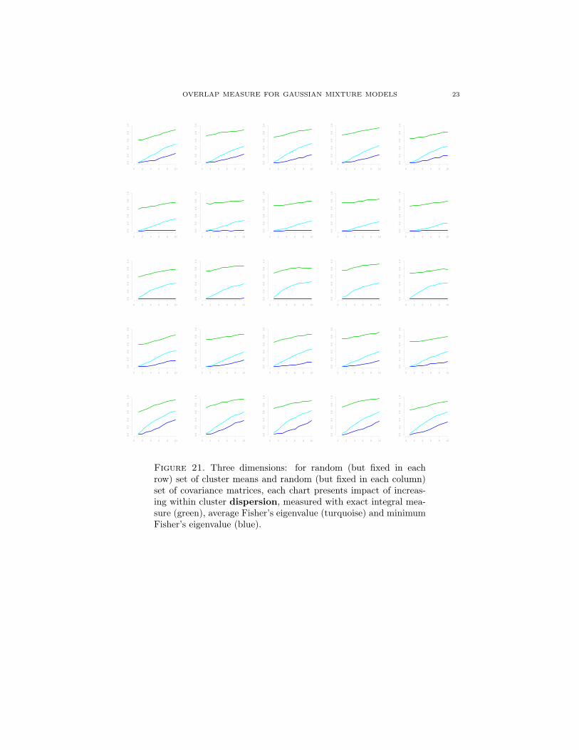
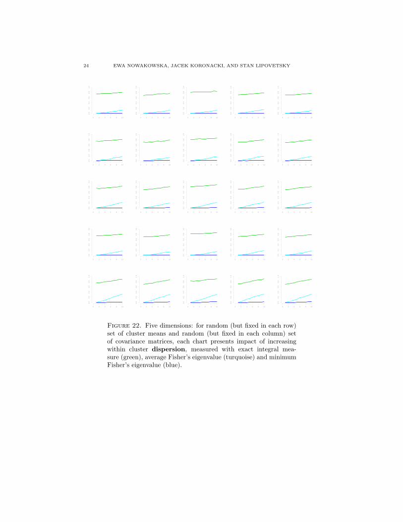
Figure 6. Effect of increasing between cluster distance (left col-umn) and within cluster dispersion (right column). Upper rowgives results for three dimensional simulations, while bottom rowfor five dimensional case. Green line indicates Monte Carlo esti-mate of the integral structure distinctness, turquoise average non-zero Fisher’s eigenvalue, while blue — Fisher’s smallest non-zeroeigenvalue.
Again, what can be observed in all the simulation plots in Appendix A is illus-trated in Figure 6. Behavior of average Fisher’s eigenvalue as given by (22) reflectsvariability of the integral measure. At the same time, minimum non-zero Fisher’seigenvalue (22) is less sensitive and therefore captures the changes in distinctness

OVERLAP MEASURE FOR GAUSSIAN MIXTURE MODELS 13
to a lesser extent, which becomes even more apparent as the number of dimensionsincreases. As such, the average non-zero Fisher’s eigenvalue tends to outperformthe minimum non-zero Fisher’s eigenvalue and therefore the former shall be recom-mended as the distinctness coefficient.
5. Conclusions.
In this work we derive and motivate measure of distinctness (or alternatively– overlap) between clusters of data, generated from a Gaussian mixture model.The approach uses alternative formulation of Fisher’s discrimination task, which isstated in terms of a generalized eigenproblem. We show the task is well posed inthe context of the assumed model and can be reduced to a standard eigenproblemwith real eigenvalues. We then express the distinctness coefficient as the averageeigenvalue over the non-zero eigenvalues of the solution. We compare the behav-ior of the coefficient with the generic (integral) measure of structure distinctnessdefined in terms of the actual overlap between the corresponding distributions andits best linear approximation. Although the values of the Fisher’s coefficient arelower than the values of actual overlap, their dynamic reflects very well the behav-ior of the generic integral measure and even better – its best linear approximation.As opposed to the generic integral measure and its best linear approximation, theFisher’s coefficient offers the advantage of being not only numerically easily com-putable but also analytically tractable, even in a complex setup, regardless of thedimensionality of the space and heterogeneity of covariance matrices.
References
[1] A. Bhattacharyya, On a measure of divergence between two statistical populations definedby their probability distributions, Bulletin of Cal. Math. Soc. 35 (1) (1943) 99–109.
[2] K. Fukunaga, Introduction to statistical pattern recognition, 2nd Edition, Computer Scienceand Scientific Computing, Academic Press, Inc., Boston, MA, 1990.
[3] N. E. Day, Estimating the components of a mixture of normal distributions, Biometrika 56 (3)(1969) 463–474.URL http://www.jstor.org/stable/2334652
[4] G. J. McLachlan, K. E. Basford, Mixture models, Vol. 84 of Statistics: Textbooks and Mono-graphs, Marcel Dekker, Inc., New York, 1988, inference and applications to clustering.
[5] S. Kullback, R. A. Leibler, On information and sufficiency, Ann. Math. Statistics 22 (1951)79–86. doi:10.1214/aoms/1177729694.
[6] H. F. Inman, E. L. Bradley, Jr., The overlapping coefficient as a measure of agreement betweenprobability distributions and point estimation of the overlap of two normal densities, Comm.Statist. Theory Methods 18 (10) (1989) 3851–3874. doi:10.1080/03610928908830127.URL http://dx.doi.org/10.1080/03610928908830127
[7] S. Dasgupta, Learning mixtures of gaussians, in: 40th Annual Symposium on Foundations ofComputer Science, 1999, pp. 634–644. doi:10.1109/SFFCS.1999.814639.
[8] R. Maitra, Initializing partition-optimization algorithms, IEEE/ACM Trans. Comput. Biol.Bioinformatics 6 (1) (2009) 144–157. doi:10.1109/TCBB.2007.70244.URL http://dx.doi.org/10.1109/TCBB.2007.70244
[9] H.-J. Sun, M. Sun, S.-R. Wang, A measurement of overlap rate between gaussiancomponents,in: International Conference on Machine Learning and Cybernetics, Vol. 4, 2007, pp. 2373–2378. doi:10.1109/ICMLC.2007.4370542.
[10] S. Ray, B. G. Lindsay, The topography of multivariate normal mixtures, Ann. Statist. 33 (5)(2005) 2042–2065. doi:10.1214/009053605000000417.URL http://dx.doi.org/10.1214/009053605000000417
[11] H. Sun, S. Wang, Measuring the component overlapping in the Gaussian mixture model,Data Min. Knowl. Discov. 23 (3) (2011) 479–502. doi:10.1007/s10618-011-0212-3.URL http://dx.doi.org/10.1007/s10618-011-0212-3

14 EWA NOWAKOWSKA, JACEK KORONACKI, AND STAN LIPOVETSKY
[12] K. V. Mardia, J. T. Kent, J. M. Bibby, Multivariate analysis, Academic Press [Harcourt BraceJovanovich, Publishers], London-New York-Toronto, Ont., 1979, probability and Mathemat-ical Statistics: A Series of Monographs and Textbooks.
[13] T. W. Anderson, R. R. Bahadur, Classification into two multivariate normal distributionswith different covariance matrices, The Annals of Mathematical Statistics 33 (2) (1962) 420–431. doi:10.1214/aoms/1177704568.URL http://dx.doi.org/10.1214/aoms/1177704568
[14] G. J. Székely, M. L. Rizzo, Hierarchical clustering via joint between-within distances: ex-tending Ward’s minimum variance method, J. Classification 22 (2) (2005) 151–183. doi:10.1007/s00357-005-0012-9.URL http://dx.doi.org/10.1007/s00357-005-0012-9
[15] J. H. Ward, Jr., Hierarchical grouping to optimize an objective function, J. Amer. Statist.Assoc. 58 (1963) 236–244. doi:10.2307/2282967.
[16] T. Hastie, R. Tibshirani, J. Friedman, The elements of statistical learning, 2nd Edition,Springer Series in Statistics, Springer, New York, 2009, data mining, inference, and prediction.doi:10.1007/978-0-387-84858-7.URL http://dx.doi.org/10.1007/978-0-387-84858-7
[17] S. Lipovetsky, Additive and multiplicative mixed normal distributions and finding clustercenters, International Journal of Machine Learning and Cybernetics 4 (1) (2013) 1–11. doi:10.1007/s13042-012-0070-3.URL http://dx.doi.org/10.1007/s13042-012-0070-3
[18] S. Lipovetsky, Total odds and other objectives for clustering via multinomial-logit model, Ad-vances in Adaptive Data Analysis 04 (03) (2012) 1250019. doi:10.1142/S1793536912500197.URL http://www.worldscientific.com/doi/abs/10.1142/S1793536912500197
[19] S. Lipovetsky, Finding cluster centers and sizes via multinomial parameterization, AppliedMathematics and Computation 221 (2013) 571–580. doi:10.1016/j.amc.2013.06.098.
[20] R. Fisher, The use of multiple measurements in taxonomic problems, Annals of Eugenics7 (2) (1936) 179–188. doi:10.1111/j.1469-1809.1936.tb02137.x.URL http://dx.doi.org/10.1111/j.1469-1809.1936.tb02137.x
[21] M. S. Bartlett, Further aspects of the theory of multiple regression, Mathematical Proceedingsof the Cambridge Philosophical Society 34 (1938) 33–40. doi:10.1017/S0305004100019897.URL http://journals.cambridge.org/article_S0305004100019897
[22] W. Dillon, M. Goldstein, Multivariate analysis: methods and applications, Wiley series inprobability and mathematical statistics: Applied probability and statistics, Wiley, 1984.
[23] S. Brubaker, S. Vempala, Isotropic pca and affine-invariant clustering, in: M. Grötschel,G. Katona, G. Sági (Eds.), Building Bridges, Vol. 19 of Bolyai Society Mathematical Studies,Springer Berlin Heidelberg, 2008, pp. 241–281. doi:10.1007/978-3-540-85221-6_8.URL http://dx.doi.org/10.1007/978-3-540-85221-6_8
[24] J. E. Gentle, Random number generation and Monte Carlo methods, 2nd Edition, Statisticsand Computing, Springer, New York, 2003.
[25] H. Joe, Generating random correlation matrices based on partial correlations, J. MultivariateAnal. 97 (10) (2006) 2177–2189. doi:10.1016/j.jmva.2005.05.010.URL http://dx.doi.org/10.1016/j.jmva.2005.05.010
[26] D. Kurowicka, R. Cooke, Uncertainty analysis with high dimensional dependence modelling,Wiley Series in Probability and Statistics, John Wiley & Sons, Ltd., Chichester, 2006. doi:10.1002/0470863072.URL http://dx.doi.org/10.1002/0470863072
OVERLAP MEASURE FOR GAUSSIAN MIXTURE MODELS 15
Appendix A. Simulation results
Ewa Nowakowska, Institute of Computer Science, Polish Academy of Sciences,ul. Jana Kazimierza 5, 01-248 Warszawa, Poland
E-mail address: [email protected]
Jacek Koronacki, Institute of Computer Science, Polish Academy of Sciences, ul.Jana Kazimierza 5, 01-248 Warszawa, Poland
E-mail address: [email protected]
Stan Lipovetsky, GfK Custom Research North America, Marketing & Data Sci-ences, 8401 Golden Valley Rd., Minneapolis MN 55427, USA
E-mail address: [email protected]

16 EWA NOWAKOWSKA, JACEK KORONACKI, AND STAN LIPOVETSKY
−5 0 5
−5
05
−5 0 5
−5
05
−5 0 5
−5
05
−5 0 5
−5
05
−5 0 5
−5
05
−5 0 5
−5
05
−5 0 5
−5
05
−5 0 5
−5
05
−5 0 5
−5
05
−5 0 5
−5
05
Figure 7. Diagram of increasing between cluster distance
0 2 4 6 8 10
0.2
0.6
1.0
0 2 4 6 8 10
0.2
0.6
1.0
0 2 4 6 8 10
0.2
0.6
1.0
0 2 4 6 8 10
0.0
0.4
0.8
0 2 4 6 8 10
0.2
0.6
1.0
0 2 4 6 8 10
0.2
0.6
1.0
0 2 4 6 8 10
0.2
0.6
1.0
0 2 4 6 8 10
0.2
0.6
1.0
0 2 4 6 8 10
0.2
0.6
1.0
0 2 4 6 8 10
0.2
0.6
1.0
0 2 4 6 8 10
0.2
0.6
1.0
0 2 4 6 8 10
0.2
0.6
1.0
0 2 4 6 8 10
0.2
0.6
1.0
0 2 4 6 8 10
0.2
0.6
1.0
0 2 4 6 8 10
0.2
0.6
1.0
0 2 4 6 8 10
0.0
0.4
0.8
0 2 4 6 8 10
0.0
0.4
0.8
0 2 4 6 8 10
0.2
0.6
1.0
0 2 4 6 8 10
0.0
0.4
0.8
0 2 4 6 8 10
0.2
0.6
1.0
0 2 4 6 8 10
0.0
0.4
0.8
0 2 4 6 8 10
0.0
0.4
0.8
0 2 4 6 8 10
0.0
0.4
0.8
0 2 4 6 8 10
0.2
0.6
1.0
0 2 4 6 8 10
0.2
0.6
1.0
0 2 4 6 8 10
0.2
0.6
1.0
0 2 4 6 8 10
0.2
0.6
1.0
0 2 4 6 8 10
0.2
0.6
1.0
0 2 4 6 8 10
0.2
0.6
1.0
0 2 4 6 8 10
0.2
0.6
1.0
0 2 4 6 8 10
0.2
0.6
1.0
0 2 4 6 8 10
0.2
0.6
1.0
0 2 4 6 8 10
0.0
0.4
0.8
0 2 4 6 8 10
0.0
0.4
0.8
0 2 4 6 8 10
0.2
0.6
1.0
0 2 4 6 8 10
0.2
0.6
1.0
Figure 8. For clusters in position as in Figure 4, each chartpresents impact of increasing between cluster distance accordingto the pattern from Figure 7, measured with exact (1 −MLEerr)(red), its linear approximation (1− Pminmax) (green) and Fisher’seigenvalue (blue).

OVERLAP MEASURE FOR GAUSSIAN MIXTURE MODELS 17
−5 0 5
−5
05
−5 0 5
−5
05
−5 0 5
−5
05
−5 0 5
−5
05
−10 −5 0 5 10
−10
−5
05
10
−10 −5 0 5 10
−10
−5
05
10
−10 −5 0 5 10
−10
−5
05
10
−10 −5 0 5 10
−10
05
10
−10 −5 0 5 10
−10
05
10
−10 −5 0 5 10
−10
05
10
Figure 9. Diagram of increasing within cluster dispersion – inboth spanning directions
0 2 4 6 8 10
0.70
0.85
1.00
0 2 4 6 8 10
0.6
0.8
1.0
0 2 4 6 8 10
0.3
0.6
0.9
0 2 4 6 8 10
0.2
0.6
0 2 4 6 8 10
0.3
0.6
0.9
0 2 4 6 8 10
0.6
0.8
1.0
0 2 4 6 8 10
0.6
0.8
0 2 4 6 8 10
0.6
0.8
1.0
0 2 4 6 8 10
0.4
0.6
0.8
0 2 4 6 8 10
0.2
0.6
0 2 4 6 8 10
0.3
0.6
0.9
0 2 4 6 8 10
0.5
0.7
0.9
0 2 4 6 8 10
0.5
0.7
0.9
0 2 4 6 8 10
0.5
0.7
0.9
0 2 4 6 8 10
0.4
0.6
0.8
0 2 4 6 8 10
0.2
0.5
0.8
0 2 4 6 8 10
0.2
0.5
0.8
0 2 4 6 8 10
0.4
0.6
0.8
0 2 4 6 8 10
0.4
0.6
0.8
0 2 4 6 8 10
0.4
0.6
0.8
0 2 4 6 8 10
0.3
0.6
0.9
0 2 4 6 8 10
0.2
0.5
0.8
0 2 4 6 8 10
0.3
0.5
0.7
0 2 4 6 8 10
0.4
0.6
0.8
0 2 4 6 8 10
0.5
0.7
0.9
0 2 4 6 8 10
0.4
0.6
0.8
0 2 4 6 8 10
0.2
0.5
0.8
0 2 4 6 8 10
0.2
0.5
0.8
0 2 4 6 8 10
0.4
0.6
0.8
0 2 4 6 8 10
0.5
0.7
0.9
0 2 4 6 8 10
0.6
0.8
0 2 4 6 8 10
0.5
0.7
0.9
0 2 4 6 8 10
0.3
0.6
0.9
0 2 4 6 8 10
0.2
0.6
0 2 4 6 8 10
0.4
0.6
0.8
0 2 4 6 8 10
0.6
0.8
1.0
Figure 10. For clusters in position as in Figure 4, each chartpresents impact of increasing within cluster dispersion (both di-rections) according to the pattern from Figure 9, measured withexact (1 −MLEerr) (red), its linear approximation (1 − Pminmax)(green) and Fisher’s eigenvalue (blue).

18 EWA NOWAKOWSKA, JACEK KORONACKI, AND STAN LIPOVETSKY
−5 0 5
−5
05
−5 0 5
−5
05
−5 0 5
−5
05
−5 0 5
−5
05
−10 −5 0 5 10
−10
−5
05
10
−10 −5 0 5 10
−10
−5
05
10
−10 −5 0 5 10
−10
−5
05
10
−10 −5 0 5 10
−10
05
10
−10 −5 0 5 10
−10
05
10
−10 −5 0 5 10
−10
05
10
Figure 11. Diagram of increasing within cluster dispersion –first spanning direction
0 2 4 6 8 10
0.80
0.90
0 2 4 6 8 10
0.65
0.85
0 2 4 6 8 10
0.4
0.7
0 2 4 6 8 10
0.2
0.6
0 2 4 6 8 10
0.4
0.7
0 2 4 6 8 10
0.65
0.80
0.95
0 2 4 6 8 10
0.65
0.80
0.95
0 2 4 6 8 10
0.75
0.85
0.95
0 2 4 6 8 10
0.5
0.7
0.9
0 2 4 6 8 10
0.2
0.6
0 2 4 6 8 10
0.3
0.6
0.9
0 2 4 6 8 10
0.5
0.7
0.9
0 2 4 6 8 10
0.5
0.7
0.9
0 2 4 6 8 10
0.60
0.75
0.90
0 2 4 6 8 10
0.6
0.8
0 2 4 6 8 10
0.2
0.5
0.8
0 2 4 6 8 10
0.3
0.6
0.9
0 2 4 6 8 10
0.4
0.6
0.8
0 2 4 6 8 10
0.4
0.6
0.8
0 2 4 6 8 10
0.4
0.6
0.8
0 2 4 6 8 10
0.3
0.5
0.7
0 2 4 6 8 10
0.2
0.5
0.8
0 2 4 6 8 10
0.4
0.6
0.8
0 2 4 6 8 10
0.4
0.6
0.8
0 2 4 6 8 10
0.5
0.7
0.9
0 2 4 6 8 10
0.4
0.6
0.8
0 2 4 6 8 10
0.3
0.6
0 2 4 6 8 10
0.2
0.5
0.8
0 2 4 6 8 10
0.6
0.8
0 2 4 6 8 10
0.60
0.75
0.90
0 2 4 6 8 10
0.70
0.85
0 2 4 6 8 10
0.5
0.7
0.9
0 2 4 6 8 10
0.3
0.6
0.9
0 2 4 6 8 10
0.2
0.6
0 2 4 6 8 10
0.5
0.7
0.9
0 2 4 6 8 10
0.75
0.85
0.95
Figure 12. For clusters in position as in Figure 4, each chartpresents impact of increasing within cluster dispersion (first direc-tion) according to the pattern from Figure 11, measured with exact(1−MLEerr) (red), its linear approximation (1−Pminmax) (green)and Fisher’s eigenvalue (blue).

OVERLAP MEASURE FOR GAUSSIAN MIXTURE MODELS 19
−5 0 5
−50
5
−5 0 5
−50
5
−5 0 5
−50
5
−5 0 5 10
−50
510
−10 0 5 10
−10
05
1015
−20 0 10 20
−20
−10
010
20
−20 0 10 20
−20
010
20
Figure 13. Diagram of increasing within cluster dispersion –second spanning direction
0 2 4 6 8
0.2
0.6
1.0
0 2 4 6 8
0.2
0.6
0 2 4 6 8
0.4
0.6
0.8
0 2 4 6 8
0.4
0.6
0.8
0 2 4 6 8
0.3
0.6
0.9
0 2 4 6 8
0.2
0.6
0 2 4 6 8
0.2
0.6
0 2 4 6 8
0.2
0.6
0 2 4 6 8
0.3
0.6
0.9
0 2 4 6 8
0.4
0.6
0.8
0 2 4 6 8
0.4
0.6
0.8
0 2 4 6 8
0.2
0.6
0 2 4 6 8
0.2
0.6
0 2 4 6 8
0.2
0.6
0 2 4 6 8
0.3
0.6
0.9
0 2 4 6 8
0.3
0.6
0.9
0 2 4 6 8
0.3
0.6
0.9
0 2 4 6 8
0.2
0.5
0.8
0 2 4 6 8
0.2
0.6
0 2 4 6 8
0.2
0.6
0 2 4 6 8
0.3
0.6
0.9
0 2 4 6 8
0.3
0.6
0.9
0 2 4 6 8
0.3
0.6
0.9
0 2 4 6 8
0.2
0.6
0 2 4 6 8
0.2
0.6
0 2 4 6 8
0.2
0.5
0.8
0 2 4 6 8
0.3
0.6
0.9
0 2 4 6 8
0.3
0.6
0.9
0 2 4 6 8
0.3
0.6
0.9
0 2 4 6 8
0.2
0.6
0 2 4 6 8
0.2
0.6
0 2 4 6 8
0.2
0.5
0.8
0 2 4 6 8
0.4
0.6
0.8
0 2 4 6 8
0.4
0.6
0.8
0 2 4 6 8
0.3
0.6
0.9
0 2 4 6 8
0.2
0.6
Figure 14. For clusters in position as in Figure 4, each chartpresents impact of increasing within cluster dispersion (second di-rection) according to the pattern from Figure 13, measured withexact (1 −MLEerr) (red), its linear approximation (1 − Pminmax)(green) and Fisher’s eigenvalue (blue).
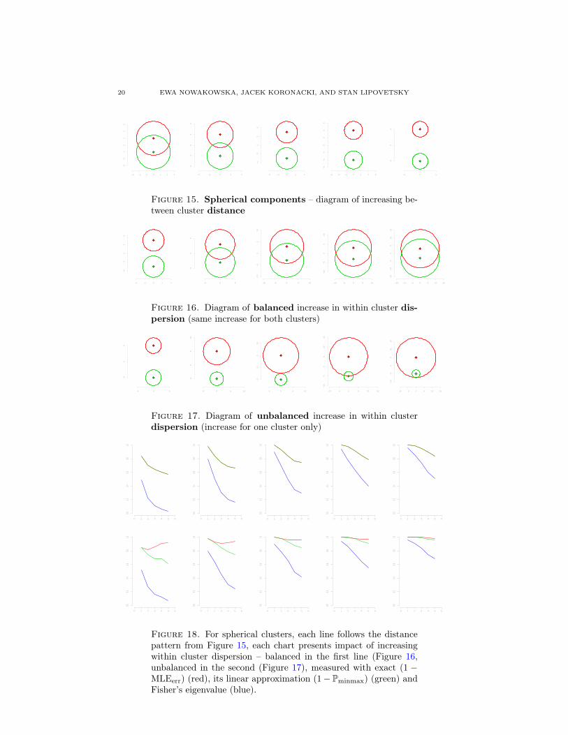
20 EWA NOWAKOWSKA, JACEK KORONACKI, AND STAN LIPOVETSKY
−3 −2 −1 0 1 2 3
−3
−2
−1
01
23
−4 −2 0 2 4
−4
−2
02
4
−4 −2 0 2 4
−4
−2
02
4
−6 −4 −2 0 2 4 6
−6
−4
−2
02
46
−5 0 5
−5
05
Figure 15. Spherical components – diagram of increasing be-tween cluster distance
−4 −2 0 2 4
−4
−2
02
4
−5 0 5
−5
05
−10 −5 0 5 10
−10
−5
05
10
−10 −5 0 5 10
−10
−5
05
10
−15 −10 −5 0 5 10 15
−15
−10
−5
05
1015
Figure 16. Diagram of balanced increase in within cluster dis-persion (same increase for both clusters)
−5 0 5
−5
05
−5 0 5 10
−5
05
10
−5 0 5 10
−5
05
10
−10 −5 0 5 10 15
−10
−5
05
1015
−10 −5 0 5 10 15−
10−
50
510
15
Figure 17. Diagram of unbalanced increase in within clusterdispersion (increase for one cluster only)
0 1 2 3 4 5 6
0.00.2
0.40.6
0.81.0
0 1 2 3 4 5 6
0.00.2
0.40.6
0.81.0
0 1 2 3 4 5 6
0.00.2
0.40.6
0.81.0
0 1 2 3 4 5 6
0.00.2
0.40.6
0.81.0
0 1 2 3 4 5 6
0.00.2
0.40.6
0.81.0
0 1 2 3 4 5 6
0.00.2
0.40.6
0.81.0
0 1 2 3 4 5 6
0.00.2
0.40.6
0.81.0
0 1 2 3 4 5 6
0.00.2
0.40.6
0.81.0
0 1 2 3 4 5 6
0.00.2
0.40.6
0.81.0
0 1 2 3 4 5 6
0.00.2
0.40.6
0.81.0
Figure 18. For spherical clusters, each line follows the distancepattern from Figure 15, each chart presents impact of increasingwithin cluster dispersion – balanced in the first line (Figure 16,unbalanced in the second (Figure 17), measured with exact (1 −MLEerr) (red), its linear approximation (1− Pminmax) (green) andFisher’s eigenvalue (blue).

OVERLAP MEASURE FOR GAUSSIAN MIXTURE MODELS 21
0 2 4 6 8 10
0.0
0.2
0.4
0.6
0.8
1.0
0 2 4 6 8 10
0.0
0.2
0.4
0.6
0.8
1.0
0 2 4 6 8 10
0.0
0.2
0.4
0.6
0.8
1.0
0 2 4 6 8 10
0.0
0.2
0.4
0.6
0.8
1.0
0 2 4 6 8 10
0.0
0.2
0.4
0.6
0.8
1.0
0 2 4 6 8 10
0.0
0.2
0.4
0.6
0.8
1.0
0 2 4 6 8 10
0.0
0.2
0.4
0.6
0.8
1.0
0 2 4 6 8 10
0.0
0.2
0.4
0.6
0.8
1.0
0 2 4 6 8 10
0.0
0.2
0.4
0.6
0.8
1.0
0 2 4 6 8 10
0.0
0.2
0.4
0.6
0.8
1.0
0 2 4 6 8 10
0.0
0.2
0.4
0.6
0.8
1.0
0 2 4 6 8 10
0.0
0.2
0.4
0.6
0.8
1.0
0 2 4 6 8 10
0.0
0.2
0.4
0.6
0.8
1.0
0 2 4 6 8 10
0.0
0.2
0.4
0.6
0.8
1.0
0 2 4 6 8 10
0.0
0.2
0.4
0.6
0.8
1.0
0 2 4 6 8 10
0.0
0.2
0.4
0.6
0.8
1.0
0 2 4 6 8 10
0.0
0.2
0.4
0.6
0.8
1.0
0 2 4 6 8 10
0.0
0.2
0.4
0.6
0.8
1.0
0 2 4 6 8 10
0.0
0.2
0.4
0.6
0.8
1.0
0 2 4 6 8 10
0.0
0.2
0.4
0.6
0.8
1.0
0 2 4 6 8 10
0.0
0.2
0.4
0.6
0.8
1.0
0 2 4 6 8 10
0.0
0.2
0.4
0.6
0.8
1.0
0 2 4 6 8 10
0.0
0.2
0.4
0.6
0.8
1.0
0 2 4 6 8 10
0.0
0.2
0.4
0.6
0.8
1.0
0 2 4 6 8 10
0.0
0.2
0.4
0.6
0.8
1.0
Figure 19. Three dimensions: for random (but fixed in eachrow) set of cluster means and random (but fixed in each column)set of covariance matrices, each chart presents impact of increas-ing between cluster distance, measured with exact integral mea-sure (green), average Fisher’s eigenvalue (turquoise) and minimumFisher’s eigenvalue (blue).

22 EWA NOWAKOWSKA, JACEK KORONACKI, AND STAN LIPOVETSKY
0 2 4 6 8 10
0.0
0.2
0.4
0.6
0.8
1.0
0 2 4 6 8 10
0.0
0.2
0.4
0.6
0.8
1.0
0 2 4 6 8 10
0.0
0.2
0.4
0.6
0.8
1.0
0 2 4 6 8 10
0.0
0.2
0.4
0.6
0.8
1.0
0 2 4 6 8 10
0.0
0.2
0.4
0.6
0.8
1.0
0 2 4 6 8 10
0.0
0.2
0.4
0.6
0.8
1.0
0 2 4 6 8 10
0.0
0.2
0.4
0.6
0.8
1.0
0 2 4 6 8 10
0.0
0.2
0.4
0.6
0.8
1.0
0 2 4 6 8 10
0.0
0.2
0.4
0.6
0.8
1.0
0 2 4 6 8 10
0.0
0.2
0.4
0.6
0.8
1.0
0 2 4 6 8 10
0.0
0.2
0.4
0.6
0.8
1.0
0 2 4 6 8 10
0.0
0.2
0.4
0.6
0.8
1.0
0 2 4 6 8 10
0.0
0.2
0.4
0.6
0.8
1.0
0 2 4 6 8 10
0.0
0.2
0.4
0.6
0.8
1.0
0 2 4 6 8 10
0.0
0.2
0.4
0.6
0.8
1.0
0 2 4 6 8 10
0.0
0.2
0.4
0.6
0.8
1.0
0 2 4 6 8 10
0.0
0.2
0.4
0.6
0.8
1.0
0 2 4 6 8 10
0.0
0.2
0.4
0.6
0.8
1.0
0 2 4 6 8 10
0.0
0.2
0.4
0.6
0.8
1.0
0 2 4 6 8 10
0.0
0.2
0.4
0.6
0.8
1.0
0 2 4 6 8 10
0.0
0.2
0.4
0.6
0.8
1.0
0 2 4 6 8 10
0.0
0.2
0.4
0.6
0.8
1.0
0 2 4 6 8 10
0.0
0.2
0.4
0.6
0.8
1.0
0 2 4 6 8 10
0.0
0.2
0.4
0.6
0.8
1.0
0 2 4 6 8 10
0.0
0.2
0.4
0.6
0.8
1.0
Figure 20. Five dimensions: for random (but fixed in each row)set of cluster means and random (but fixed in each column) setof covariance matrices, each chart presents impact of increas-ing between cluster distance, measured with exact integral mea-sure (green), average Fisher’s eigenvalue (turquoise) and minimumFisher’s eigenvalue (blue).
OVERLAP MEASURE FOR GAUSSIAN MIXTURE MODELS 23
0 2 4 6 8 10
0.0
0.2
0.4
0.6
0.8
1.0
0 2 4 6 8 10
0.0
0.2
0.4
0.6
0.8
1.0
0 2 4 6 8 10
0.0
0.2
0.4
0.6
0.8
1.0
0 2 4 6 8 10
0.0
0.2
0.4
0.6
0.8
1.0
0 2 4 6 8 10
0.0
0.2
0.4
0.6
0.8
1.0
0 2 4 6 8 10
0.0
0.2
0.4
0.6
0.8
1.0
0 2 4 6 8 10
0.0
0.2
0.4
0.6
0.8
1.0
0 2 4 6 8 10
0.0
0.2
0.4
0.6
0.8
1.0
0 2 4 6 8 10
0.0
0.2
0.4
0.6
0.8
1.0
0 2 4 6 8 10
0.0
0.2
0.4
0.6
0.8
1.0
0 2 4 6 8 10
0.0
0.2
0.4
0.6
0.8
1.0
0 2 4 6 8 10
0.0
0.2
0.4
0.6
0.8
1.0
0 2 4 6 8 10
0.0
0.2
0.4
0.6
0.8
1.0
0 2 4 6 8 10
0.0
0.2
0.4
0.6
0.8
1.0
0 2 4 6 8 10
0.0
0.2
0.4
0.6
0.8
1.0
0 2 4 6 8 10
0.0
0.2
0.4
0.6
0.8
1.0
0 2 4 6 8 10
0.0
0.2
0.4
0.6
0.8
1.0
0 2 4 6 8 10
0.0
0.2
0.4
0.6
0.8
1.0
0 2 4 6 8 10
0.0
0.2
0.4
0.6
0.8
1.0
0 2 4 6 8 10
0.0
0.2
0.4
0.6
0.8
1.0
0 2 4 6 8 10
0.0
0.2
0.4
0.6
0.8
1.0
0 2 4 6 8 10
0.0
0.2
0.4
0.6
0.8
1.0
0 2 4 6 8 10
0.0
0.2
0.4
0.6
0.8
1.0
0 2 4 6 8 10
0.0
0.2
0.4
0.6
0.8
1.0
0 2 4 6 8 10
0.0
0.2
0.4
0.6
0.8
1.0
Figure 21. Three dimensions: for random (but fixed in eachrow) set of cluster means and random (but fixed in each column)set of covariance matrices, each chart presents impact of increas-ing within cluster dispersion, measured with exact integral mea-sure (green), average Fisher’s eigenvalue (turquoise) and minimumFisher’s eigenvalue (blue).
24 EWA NOWAKOWSKA, JACEK KORONACKI, AND STAN LIPOVETSKY
0 2 4 6 8 10
0.0
0.2
0.4
0.6
0.8
1.0
0 2 4 6 8 10
0.0
0.2
0.4
0.6
0.8
1.0
0 2 4 6 8 10
0.0
0.2
0.4
0.6
0.8
1.0
0 2 4 6 8 10
0.0
0.2
0.4
0.6
0.8
1.0
0 2 4 6 8 10
0.0
0.2
0.4
0.6
0.8
1.0
0 2 4 6 8 10
0.0
0.2
0.4
0.6
0.8
1.0
0 2 4 6 8 10
0.0
0.2
0.4
0.6
0.8
1.0
0 2 4 6 8 10
0.0
0.2
0.4
0.6
0.8
1.0
0 2 4 6 8 10
0.0
0.2
0.4
0.6
0.8
1.0
0 2 4 6 8 10
0.0
0.2
0.4
0.6
0.8
1.0
0 2 4 6 8 10
0.0
0.2
0.4
0.6
0.8
1.0
0 2 4 6 8 10
0.0
0.2
0.4
0.6
0.8
1.0
0 2 4 6 8 10
0.0
0.2
0.4
0.6
0.8
1.0
0 2 4 6 8 10
0.0
0.2
0.4
0.6
0.8
1.0
0 2 4 6 8 10
0.0
0.2
0.4
0.6
0.8
1.0
0 2 4 6 8 10
0.0
0.2
0.4
0.6
0.8
1.0
0 2 4 6 8 10
0.0
0.2
0.4
0.6
0.8
1.0
0 2 4 6 8 10
0.0
0.2
0.4
0.6
0.8
1.0
0 2 4 6 8 10
0.0
0.2
0.4
0.6
0.8
1.0
0 2 4 6 8 10
0.0
0.2
0.4
0.6
0.8
1.0
0 2 4 6 8 10
0.0
0.2
0.4
0.6
0.8
1.0
0 2 4 6 8 10
0.0
0.2
0.4
0.6
0.8
1.0
0 2 4 6 8 10
0.0
0.2
0.4
0.6
0.8
1.0
0 2 4 6 8 10
0.0
0.2
0.4
0.6
0.8
1.0
0 2 4 6 8 10
0.0
0.2
0.4
0.6
0.8
1.0
Figure 22. Five dimensions: for random (but fixed in each row)set of cluster means and random (but fixed in each column) setof covariance matrices, each chart presents impact of increasingwithin cluster dispersion, measured with exact integral mea-sure (green), average Fisher’s eigenvalue (turquoise) and minimumFisher’s eigenvalue (blue).