Embed Size (px)
Citation preview
Practical Assessment, Research, and Evaluation Practical Assessment, Research, and Evaluation
Volume 24 Volume 24, 2019 Article 4
2019
Overview and Illustration of Bayesian Confirmatory Factor Overview and Illustration of Bayesian Confirmatory Factor
Analysis with Ordinal Indicators Analysis with Ordinal Indicators
John M. Taylor
Follow this and additional works at: https://scholarworks.umass.edu/pare
Recommended Citation Recommended Citation Taylor, John M. (2019) "Overview and Illustration of Bayesian Confirmatory Factor Analysis with Ordinal Indicators," Practical Assessment, Research, and Evaluation: Vol. 24 , Article 4. DOI: https://doi.org/10.7275/vk6g-0075 Available at: https://scholarworks.umass.edu/pare/vol24/iss1/4
This Article is brought to you for free and open access by ScholarWorks@UMass Amherst. It has been accepted for inclusion in Practical Assessment, Research, and Evaluation by an authorized editor of ScholarWorks@UMass Amherst. For more information, please contact [email protected].
A peer-reviewed electronic journal.
Copyright is retained by the first or sole author, who grants right of first publication to Practical Assessment, Research & Evaluation. Permission is granted to distribute this article for nonprofit, educational purposes if it is copied in its entirety and the journal is credited. PARE has the right to authorize third party reproduction of this article in print, electronic and database forms.
Volume 24 Number 4, May 2019 ISSN 1531-7714
Overview and Illustration of Bayesian Confirmatory Factor Analysis with Ordinal Indicators
John M. Taylor, Saint Louis University
Although frequentist estimators can effectively fit ordinal confirmatory factor analysis (CFA) models, their assumptions are difficult to establish and estimation problems may prohibit their use at times. Consequently, researchers may want to also look to Bayesian analysis to fit their ordinal models. Bayesian methods offer researchers an effective means of estimating, testing, and interpreting ordinal CFA models. Unfortunately, there are few applied resources on the subject. The purpose of this article is to provide researchers with an introduction to the essential concepts, practice recommendations, and process of fitting ordinal CFA models using Bayesian analysis. Mplus 7.4 and data from the Pittsburg Common Cold Study 3 are used to example how researchers can set up their Bayesian models, conduct diagnostic checks, and interpret the results. This article also highlights the benefits and challenges of Bayesian ordinal CFA modeling.
Confirmatory factor analysis (CFA) is typically conducted using Maximum Likelihood (ML) estimators that assume the observed data are continuous and multivariate normal (Flora & Curran, 2004; Jöreskog & Moustaki, 2001). However, since response variables are often measured using rating scales, normal-theory CFA assumptions go unmet at times (Flora & Curran, 2004; Jöreskog & Moustaki, 2001). Rating scales divide up a continuous scale into a few forced-choice response categories that are ordinally arranged relative to the underlying continuous response variable that the researcher wishes to address (Brown, 2015; DiStefano, 2002). When the ordinality of rating scale data is ignored in a CFA study several unwanted problems may ensue. For example, Beauducel and Herzberg (2006) found that slope parameters tend to be attenuated when rating scales with six response options or less are treated as continuous in ML estimation while Bandalos (2014) found that standard errors tend to be negatively biased when rating scales with four response options or less are treated as continuous. Likewise, Holgado-Tello, Chacón–Moscoso, Barbero-García, and Vila-Abad (2010) found that the normal-theory χ2 statistic tends to be inflated when rating scales with five response options are treated as continuous.
In general, researchers have looked to robust ML and limited-information estimators when the ordinal scale of one or more indicators is expected to influence a model (Bainter, 2017; Bandalos, 2014). Unfortunately, the assumptions of both estimator families are difficult to establish (Fox, 2010) and their use can be prohibited at times (e.g., convergence failures). Given such circumstances, researchers may also want to look to Bayesian methods to effectively estimate their ordinal models, which tends to have fewer limitations than ML and limited-information estimators (Depaoli & van de Schoot, 2017). Unfortunately, Bayesian methodology has made few inroads into the CFA literature, partly because there are few resources available to help applied researchers navigate a methodology that is largely unfamiliar to them and complex (Wagenmakers et al., 2018). The purpose of this article is to provide researchers with an accessible overview and demonstration on estimating, evaluating, and interpreting ordinal CFA models using Bayesian methodology.
Frequentist Estimators
Various techniques have been developed to help address some of the challenges associated with fitting
1
Taylor: Overview and Illustration of Bayesian Confirmatory Factor Analysi
Published by ScholarWorks@UMass Amherst, 2019
Practical Assessment, Research & Evaluation, Vol 24 No 4 Page 2 Taylor, Bayesian Ordinal CFA Modeling CFA models when normal theory assumptions go unmet (e.g., bootstrapping; Loehlin, 2004). Particular emphasis has been placed on robust ML estimation, which attempts to repair the deleterious impact of multivariate nonnormality (Bandalos, 2014; Li, 2016). Although several variants exist, robust ML generally consists of a correction to the normal-theory χ2 using an estimate of excessive multivariate kurtosis – referred to as the scaling correction factor (Bryant & Sattora, 2012; Yuan, Bentler, & Zhang, 2005) – and a correction for kurtosis in the standard errors (Enders, 2010). However, there is some counterindication for the use of robust ML with ordinal indicators. Yang-Wallentin, Jöreskog, and Luo (2010, p. 398) noted that the use of normal theory estimators with ordinal indicators is theoretical unjustified and as the indicators become increasingly inconsistent with multivariate normality, simulation studies have found that robust ML estimators tend to produce inadmissible solutions, biased loading estimates, and inflated type I error rates (Rhemtulla, Brosseau-Liard, & Savalei, 2012; Yang-Wallentin et al., 2010).
Methodologists tend to encourage researchers to use limited-information estimators when CFA models include ordinally scaled indicators (e.g., Holgado-Tello et al., 2010). In particular, robust weighted least squares, robust unweighted least squares, and robust diagonally weighted least squares have been viewed favorably owing to their use of corrections similar to those in robust ML and their ability to model the ordinality of rating scale data (DiStefano & Morgan, 2014; Yang-Wallentin et al., 2010). Although limited-information estimators tend to perform well (e.g., Rhemtulla et al., 2012; Yang-Wallentin et al., 2010), they are not problem free. For example, limited-information estimators may perform poorly when cell counts are sparse (e.g., Forero & Maydeu-Olivares, 2009), a scenario relatively common in ordinal data. Accordingly, applied researchers would benefit from additional approaches that are not restricted by the same limitations as robust ML and limited-information estimation.
Introduction to Bayesian Estimation
Robust ML and limited-information estimators represent orthodox, or frequentist, approaches to estimation (Dienes, 2011). In frequentists estimation, unknown parameters are treated as fixed values that are estimable by identifying quantities that most likely explain the observed data (Myung, 2003). The likelihood
of parameter θ given the observed data is commonly denoted as L(θ|data). In contrast, Bayesian estimation treats unknown parameters as random variables through the assignment of probability distributions, or priors, which quantify a researcher’s prior beliefs about the credibility of different values for θ (Kaplan & Depaoli, 2012). The priors are weighted by the L(θ|data), or the evidence supplied by the data, to give researchers updated, or posterior probabilities that summarize the evidence for various values of θ (Enders, 2010; Kaplan & Depaoli, 2012; Kruschke, 2014). This core philosophy is known as Bayes’ Theorem (Lynch, 2007, p. 232):
p(θ|data) ∝ L(θ|data) p(θ) (1)
where the posterior distribution p(θ|data) is proportional to the product of the likelihood L(θ|data) and prior distribution p(θ) (Enders, 2010; Lynch, 2007).
Priors are a distinguishing feature of Bayesian statistics as well as a source of much controversy (Pawitan, 2001). Both the type of distribution and distribution parameters are set by the researcher, and based upon those choices, priors may be classified as noninformative, weakly informative or informative (Gelman, Stern, Carlin Dunson, Vehtari, & Rubin, 2014; Kaplan & Depaoli, 2012). Noninformative priors express a high degree of uncertainty over the plausible values for θ and, consequently, are expected to have trivial influence over the posterior, allowing the observed data to determine the posterior probabilities (Gelman et al., 2014; Kruschke, 2014). For example, in a CFA of the Parent/Caregiver Involvement Scale, Taylor and Bergin (2019) assigned a uniform prior over -∞ and ∞ on all interfactor correlations in order to give no more weight to one correlation estimate over another prior to introducing the evidence supplied by the data. It is worth cautioning though, noninformative priors may still have an unexpected influence over the posterior probabilities and so researchers need to carefully select and justify their priors, regardless of their level of informativeness (Depaoli & van de Schoot, 2017; Seaman, Seaman, & Stamey, 2012).
Comparatively, weakly informative and informative priors are expected to have an impact on the posterior probabilities (Gelman et al., 2014). Weakly informative priors convey a substantial degree of uncertainty about θ but may supply enough information to keep estimates reasonable (Gelman et al., 2014; Taylor, 2019). For example, standardized loading estimates outside of -1
2
Practical Assessment, Research, and Evaluation, Vol. 24 [2019], Art. 4
https://scholarworks.umass.edu/pare/vol24/iss1/4DOI: https://doi.org/10.7275/vk6g-0075
Practical Assessment, Research & Evaluation, Vol 24 No 4 Page 3 Taylor, Bayesian Ordinal CFA Modeling and +1 are unlikely and assigning a standardized indicator a uniform prior over the range of -2 to +2 could be described as weakly informative since it only rejects posterior estimates outside of -2 or +2 and assigns equal probability to loading estimates between -2 and +2 (Brown, 2015; Merkle & Rosseel, 2018). Informative priors on the other hand, allows researchers to substantially inform the posterior probabilities – though the influence of an informative prior diminishes as sample size increases (Kaplan & Depaoli, 2012; Lawson, 2013; Lynch, 2007). For example, Muthén and Asparouhov (2012) have pointed out that CFA models may benefit from placing small-variance (e.g., 0.001) normal priors on the cross-loadings with the mass centered over zero in order to accommodate for sampling error while keeping estimates aligned with a researcher’s belief that the parameters are essentially zero.
Once a researcher specifies the priors, the posteriors probabilities are obtained so that the parameters can be defined (Lee, 2007). In ordinal CFA models, the goal is to obtain estimates from the joint posterior distribution p(τ, θ, ξ, Y*| data), where τ , θ, ξ, and Y* are the latent thresholds, model parameters, latent variables, and latent response variables, respectively (Lee, 2007; Natesan, 2015). However, since the joint distribution is intractable to solve, Gibbs sampling is typically used to approximate the posteriors (Lee, 2007; Lynch, 2007). Gibbs sampling is a type of Markov chain Monte Carlo (MCMC) technique that approximates the posterior probabilities by simulating values from the probability distribution of one set of components at a time (e.g., thresholds) given the state of all other components and sequentially improving the values towards a desired posterior distribution (Gelman et al., 2014; Lee, 2007). The collection of sequential draws is called a Markov chain (Kruschke, 2014). Random start values are assigned to the components in order to initiate the Markov chains and over a sufficiently large number of iterations the sequence converges, or samples from the desired posterior distribution (Lee, 2007). Once the Markov chains have converged, the parameters can be approximated by empirically summarizing the posterior distributions on a subset of the simulated values – since the initial iterations are not representative of their posterior distributions they are discarded as burn-in (Lee, 2007). For example, the mean of a simulated posterior distribution can serve
as the Bayesian estimate of a loading parameter (Lee, 2007).
Benefits and Challenges of Bayesian Estimation
Bayesian estimation promises several benefits over frequentist estimators, largely conferred through the use of priors. For example, the inclusion of increasingly informative priors has been associated with improved parameter estimates over that of ML and limited-information estimators and priors have the advantage of allowing a researcher to incorporate their predictions into the estimation process (Depaoli & van de Schoot, 2017; Natesan, 2015). Likewise, since priors alleviate Bayesian latent variable modeling of the identification restrictions that limit frequentists approaches, researchers can estimate models otherwise prohibited under ML and limited-information estimation (Muthén & Asparouhov, 2012). Perhaps foremost, frequentist estimators rely on asymptotic assumptions that researchers may not be able to establish while Bayesian approaches generally mitigate the reliance on large-sample theory since MCMC algorithms allow the posterior distributions to be analyzed directly (Fox, 2010; Lynch, 2007).
Still, Bayesian methodology has made few inroads in the CFA literature. Some researchers are hesitant to adopt Bayesian methods due to the use of priors (Gelman, 2008), which has been criticized for introducing too much subjectivity into the research process (Lynch, 2007; Pawitan, 2001). Bayesian factor analysis is also not as accessible to applied researchers as frequentists estimators. For example, researchers are rarely trained on Bayesian statistics (e.g., Aiken, West, & Millsap, 2008) and few latent variable modeling programs offer Bayesian estimation and only Mplus (Muthén & Muthén, 1998-2015) and Amos (Arbuckle, 2017) are capable of fitting Bayesian CFA models with ordinal indicators. Both are relatively recent software developments. Likewise, Bayesian modeling is relatively complex and there are few educational resources in general on Bayesian CFA and even fewer still on fitting ordinal models - this author is only aware of a few chapters in Lee (2007) that provides some instruction on the subject. Accordingly, there remains a need for applied resources that can help researchers capitalize on the advantages of Bayesian methodology in their ordinal CFA studies.
3
Taylor: Overview and Illustration of Bayesian Confirmatory Factor Analysi
Published by ScholarWorks@UMass Amherst, 2019
Practical Assessment, Research & Evaluation, Vol 24 No 4 Page 4 Taylor, Bayesian Ordinal CFA Modeling
Empirical Example
Participants
To example the use of Bayesian CFA with ordinal indicators, the present article reports on a factor analysis of the ten item Perceived Stress Scale (PSS-10) using data from the Pittsburg Cold Study 3 (PCS-3; Laboratory for the Study of Stress, Immunity, and Disease, 2016). The Laboratory for the Study of Stress, Immunity, and Disease at Carnegie Mellon University collected responses to the items from 213 participants under the directorship of Sheldon Cohen, Ph.D (grant number NCCIH AT006694). Readers can access the data by downloading the file pcs3.data_012016.sav from the Common Cold Project website (www.commoncoldproject.com). Participants ages ranged from 18 to 55 years with a median age of 25. Approximately 57.7% (n = 123) were male while 42.3% (n = 90) were female. Nearly all of the respondents identified as White (66.7%, n = 142) or as Black (27.2%, n = 58). Approximately 23.0% (n = 49) had a high school education or less, 50.7% (n = 108) had completed some college or an associate degree, and 25.4% (n = 54) had a Bachelor’s degree or higher. Approximately 60.1% (n = 128) were working full or part-time at the time of the study while 39.9% (n = 85) reported they were unemployed. Lastly, family income ranged from $2,500 to $162,500 with a median income of $12,500.
Measure
The Perceived Stress Scale (PSS-10) is a popular measure of the degree to which respondents view the stress in their lives as excessive (Cohen, Kamarck, & Mermelstein, 1983; Taylor, 2015). Six items address a respondent’s perceived helplessness towards their stressors and four items address a respondent’s perceived self-efficacy (Roberti, Harrington, & Storch, 2006; Taylor, 2015). Respondents indicate on a scale ranging from 1 (Never) to 5 (Very often) how frequently in the past month their experience with stress have looked like the experiences described by the items. (Cohen et al. 1983). The PSS-10 is scored by reverse coding the four self-efficacy items and then summing across the items by subscale (Cohen et al., 1983; Taylor, 2015). High scores on both the helplessness and self-efficacy subscales are indicative of problematic levels of perceived stress (Taylor, 2015). Consistent with previous studies (e.g., Roberti et al., 2006), the estimated omega
reliabilities for scores on the perceived helplessness and self-efficacy subscales were .853 and .777, respectively.
Bayesian Data Analysis
Mplus 7.4 (Muthén & Muthén, 1998-2015) was used to conduct a Bayesian analysis on the two factor model that purportedly underlies the PSS-10 (Taylor, 2015; Appendix B provides readers with a brief guide to fitting a similar model using the Metropolis algorithm in Amos 25.0). Six items that appear to address perceived helplessness were regressed onto an initial latent factor while four items that appear to address perceived self-efficacy were regressed onto a second latent factor (Taylor, 2015). In keeping with Gelman et al. (2014), analysis of the two factor model was organized around three steps (p. 3):
1) Set up the full probability model, including the priors.
2) Estimate the posterior distributions.
3) Evaluate the appropriateness of the model and interpret the results.
Step one. As indicated above, the posterior distributions are obtained by sampling sequentially from the conditional densities of each set of model components using an MCMC algorithm (Lee, 2007). For example, the successive samples for the set of threshold parameters τ are simulated from the conditional density p(τi+1 | data, Yi*, ξi, Λi, Φi, Θi) at iteration i+1 given the state of all other components in the model at iteration i, where Yi* are the values for the set of unobserved continuous response variables underlying the ordinal data, ξi denotes the latent variables, Λi denotes the loading parameters, Φi denotes the covariance matrix of the latent factors, and Θi denotes the residual covariance matrix (Song & Lee, 2001, p. 241). Both the probit and logit links have been used to simulate values from the condition densities of ordinal CFA models (e.g., Natesan, 2015; Taylor, 2019); however, the probit model may be substantively preferred over the logit since ordinal CFA models and the probit link both assume the ordinal endogenous variables are discrete forms of an underlying continuous response variable (Jöreskog & Moustaki, 2001; Kruschke, 2014). Only the probit model is available in Mplus 7.4 (Asparouhov & Muthén, 2010b).
In order for the MCMC algorithm to sample from the conditional densities, researchers must place priors
4
Practical Assessment, Research, and Evaluation, Vol. 24 [2019], Art. 4
https://scholarworks.umass.edu/pare/vol24/iss1/4DOI: https://doi.org/10.7275/vk6g-0075
Practical Assessment, Research & Evaluation, Vol 24 No 4 Page 5 Taylor, Bayesian Ordinal CFA Modeling on the thresholds, factor loadings, and latent variance-covariance matrix (Lee, 2007). Depaoli and van de Schoot (2017) and Berger (2006) summarized that researchers may want to select their priors using guidance from substantive experts, prior publications, Bayesian philosophies (e.g., objective versus subjective philosophies), or from relevant datasets (e.g., secondary data). In addition, some researchers opt to use their own data to inform their priors, for example, using frequentist estimates of their model parameters to construct priors for a subsequent Bayesian analysis (Berger, 2006; Depaoli & van de Schoot, 2017). However, data-dependent priors have garnered much criticism among Bayesians, largely on the grounds that it violates some of the tenets of Bayesian philosophy (e.g., Berger, 2006). The present work opted to use priors that demonstrate their practical role in ordinal CFA modeling.
Generally, normal priors are placed on the loadings and thresholds while an Inverse Wishart (IW) prior is placed on the latent covariance matrix1 (e.g., Asparouhov & Muthén, 2010a; Lee, 2007; Natesan, 2015). Asparouhov and Muthén (2010a) found that loading parameters tend to be biased under increasingly diffuse priors and Gibbs sampling, especially when sample sizes are small. Accordingly, the present work set the location and scale of the loading priors to zero and one in keeping with the findings of Asparouhov and Muthén, (2010a). A N(0, 1.00) prior is viewed as weakly informative since it places 95% of a prior’s mass on a standardized loading coefficient between ±1.96√1.0 (Muthén & Asparouhov, 2012). Likewise, an IW(I, p + 1) prior was placed on the latent covariance matrix, where I is the identity matrix and p is the number of latent factors in the model, which implies a uniform probability for all realistic interfactor correlation values (Asparouhov & Muthén, 2010a). The IW(I, p + 1) is a common weakly informative prior (Alvarez, Niemi, & Simpson, 2014) and is the default setting in Mplus 7.4 (Asparouhov and Muthén, 2010b). Since a two factor model was fit to the data, a IW(I, 2 + 1) prior was placed on the latent covariance matrix. Lastly, since thresholds are generally not involved in model comparisons, Lee (2007) recommends assigning increasingly diffuse priors
1 Note, in Mplus 7.4 the residual covariance matrix Θ does not receive a prior since the residuals
to these “nuisance parameters” (p. 157). Accordingly, the location and scale of the normal priors on the thresholds were keep at the default setting in Mplus 7.4 of zero and 1010 (Asparouhov & Muthén, 2010b, p. 34).
Step Two. Consistent with the recommendations of Lee (2007), Gibbs sampling was used to simulate values from the conditional densities of the two factor model, as implemented in Mplus 7.4 (see the Appendix for an example of the Mplus 7.4 syntax used in this study). Although Gibbs sampling may be preferred in the ordinal CFA literature, researchers may want to look to other samplers (e.g., Hamiltonian Monte Carlo; Bainter, 2017) if Gibbs sampling does not meet their estimation needs (e.g., poor convergence; Lynch, 2007). As an alternative, researchers typically look to Metropolis-Hastings, which samples from the full joint posterior distribution rather than the conditionals (Lynch, 2007). Metropolis-Hastings is usually less efficient and slower than Gibbs sampling, however, it is likely to work when Gibbs sampling does not (Lynch, 2007). Metropolis-Hastings can be requested in Mplus 7.4 by setting ALGORTHIM to MH (Muthén & Muthén, 1998-2015).
Researchers must also select the number of draws to simulate from the posterior distributions. Research by Lee, Song, and Cai (2010) found that ordinal CFA models may converge after 15,000 iterations (p. 291). However, Lee et al. (2010) also indicated that the limited information provided by categorical indicators may necessitate lengthening the number of iterations in order for the chains to converge. For example, Depaoli and van de Shoot (2015) noted that increasingly complex models may need as many as a million post burn-in iterations to converge (p. 247) and an ordinal CFA study by Taylor (2019) used 100,000 post burn-in iterations to ensure adequate sampling from the posterior distributions. Consequently, the present study requested 100,000 post burn-in iterations by specifying FBITERATION=200000 in the Mplus 7.4 syntax (see Appendix) – Mplus 7.4 discards the initial half of the iterations as burn-in (Muthén, 2010).
Step Three. Once the chains have finished iterating, researchers need to inspect the posterior solutions for conditions that may undermine the validity
are a function of the loading coefficients rather than parameters (Muthén, 2016).
5
Taylor: Overview and Illustration of Bayesian Confirmatory Factor Analysi
Published by ScholarWorks@UMass Amherst, 2019
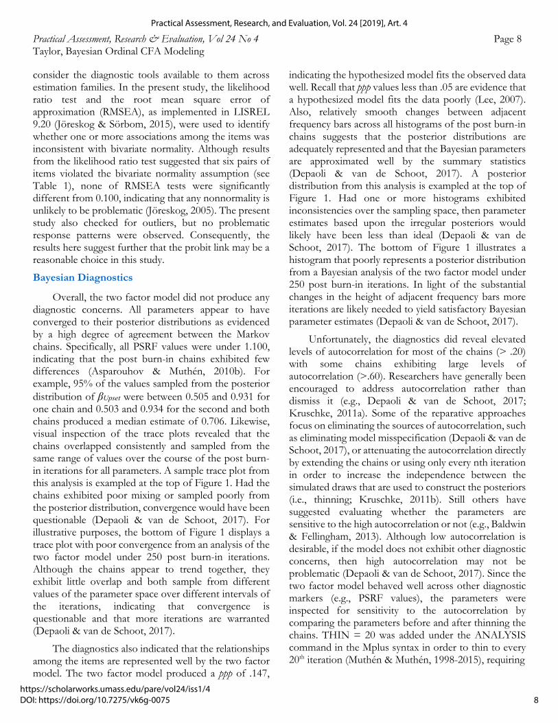
Practical Assessment, Research & Evaluation, Vol 24 No 4 Page 6 Taylor, Bayesian Ordinal CFA Modeling of their models, including (1) poor convergence, (2) elevated autocorrelation, (3) sensitivity to the priors, (4) poor representation of the posterior, and (5) model-data misfit (Depaoli & van de Schoot, 2017; Lee, 2007). Convergence for each parameter can be assessed by requesting multiple Markov chains and evaluating their consistency using the potential scale reduction factor (PSRF) and trace plots (Lee, 2007). Two chains were requested for each parameter in this study by specifying PROCESSORS=2 in the syntax (Muthén, 2010; see Appendix). The PSRF allows researchers to compare the between chain variability to the total chain variability on a given parameter (Asparouhov & Muthén, 2010b). If the between variability is relatively high (e.g., PSRF > 1.10; Lee, 2007), convergence may be poor and extending the chains further may improve convergence (Depaoli & van De Schoot, 2017; Gelman et al., 2014). Trace plots can also be inspected for convergence (Kruschke, 2014). If multiple chains are requested, then the simulated values from each chain can be superimposed in a single trace plot to visually assess for consistency (Kruschke, 2014). The x-axis on a trace plot denotes iteration length and the y-axis denotes the parameter space a sampler simulates values from (Lynch, 2007). If the chains exhibit consistent overlap and stable sampling from the same range of values over the course of the post burn-in iterations, then the parameter has likely converged to the target distribution (Kruschke, 2014). For example, the Markov chains displayed in the trace plot at the top of Figure 1 exhibit considerable overlap and the trajectory of the chains remains consistent over the course of the iterations, indicating the parameter has converged to the posterior distribution (Kruschke, 2014).
The post burn-in chains can also be displayed in a histogram in order to assess how well the posterior distribution is represented (Depaoli & van de Schoot, 2017; Kruschke, 2014). If there are small change in the heights between adjacent frequency bars over the parameter space, which is denoted on the x-axis, then summary statistics of the posterior (e.g., mean, median, standard deviation) are expected to serve as good estimates of the model parameters (Depaoli & van de Schoot, 2017). The posterior distribution exampled at the top of Figure 1 shows gradual changes in the heights between adjacent frequencies bars across the parameter space, indicating the posterior distribution is represented well (Depaoli & van de Schoot, 2017). Had the histogram periodically exhibited appreciable differences
between adjacent frequency bars, more iterations would have been warranted to improve the item’s Bayesian parameters (e.g., standard error; Depaoli & van de Schoot, 2017).
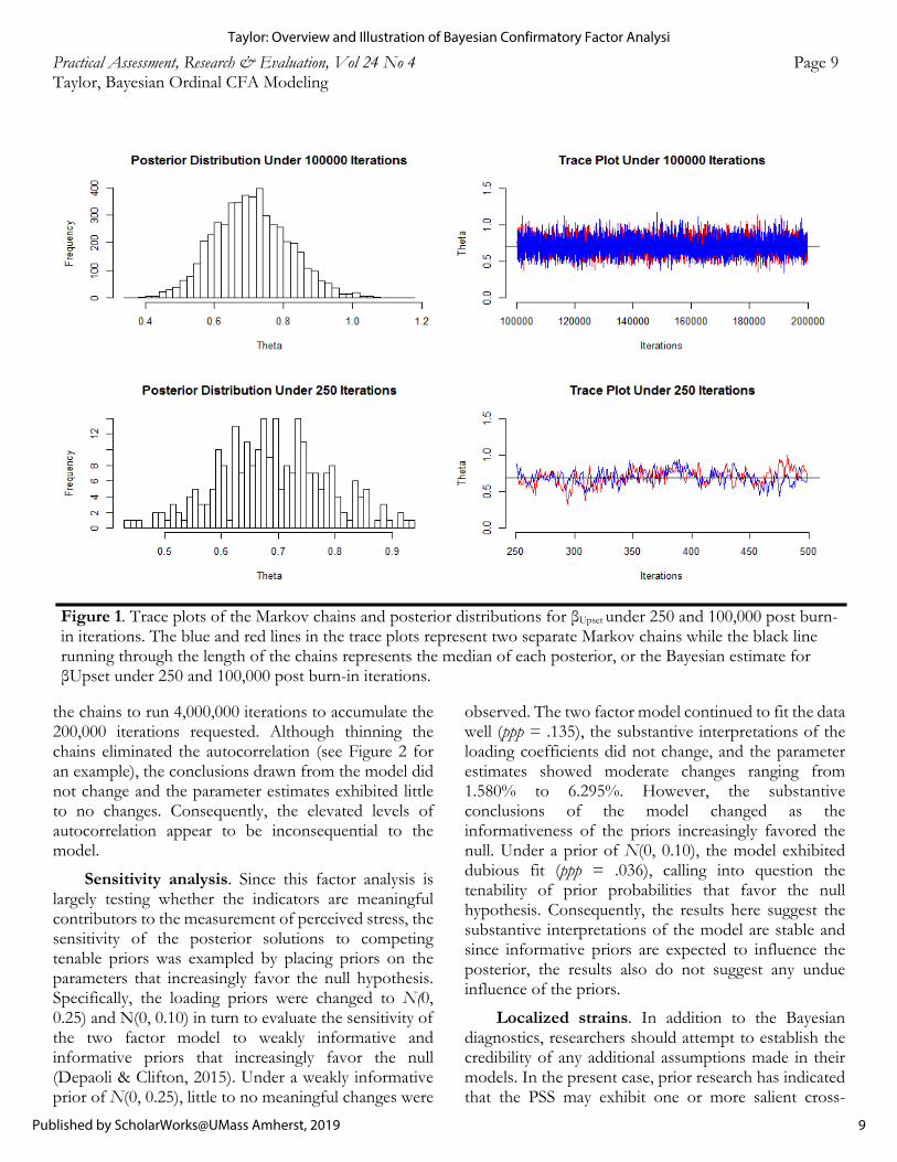
Since MCMC algorithms simulate a new estimate using the current state of a chain, the values between iterations are interrelated and the MCMC chains are autocorrelated (Lynch, 2007). If autocorrelation is excessive the target distribution may be poorly represented (Kruschke, 2014; Muthén, 2010). For example, the variability of a posterior distribution tends to be underestimated (Lynch, 2007). Autocorrelation in the MCMC chains is typically checked using autocorrelation plots (see Figure 2). The y-axis on an autocorrelation plot denotes the estimated size of the autocorrelation between the simulated values at iteration i and n iterations ahead and the x-axis denotes lags, or the intervals between post burn-in draws where the autocorrelation was checked (Lynch, 2007). Autocorrelation is expected to decrease as the lags become increasingly large, indicating the chain eventually sampled well from the posterior distribution (Pullenayegum & Thabane, 2009). However, high autocorrelation (e.g., >.10; Muthén, 2010) across increasingly large lags may be problematic and more iterations may be needed to ameliorate the problem (Depaoli & van de Schoot, 2017).
In order to test for model-data misfit, Lee (2007) has recommended using posterior predictive p-values (ppp). The ppp denotes the proportion of post burn-in iterations with a set of parameters that reflects the data poorly (Lee, 2007; Muthén & Asparouhov, 2012; Taylor, 2015). If the ppp value is too low then the model under evaluation does not fit the data well (Lee, 2007). Currently, there is a paucity of information as to what constitutes a low ppp value; however, there appears to be some agreement that ppp values close to .50 imply good fit while values less than .05 may indicate poor fit (Lee, 2007; Muthén & Asparouhov, 2012). If a model fits the data poorly, researchers may want to consider competing theoretical models.
Lastly, the sensitivity of a model to the priors should also be assessed by comparing the posteriors under competing tenable priors (Depaoli & van de Schoot, 2017; Gelman et al., 2014). Although problematic sources of sensitivity, such as poor convergence, should be addressed, the aim of a sensitivity analysis is to gain insight into the role of the priors in a given model (Depaoli & van de Schoot, 2017, Gelman et al., 2014).
6
Practical Assessment, Research, and Evaluation, Vol. 24 [2019], Art. 4
https://scholarworks.umass.edu/pare/vol24/iss1/4DOI: https://doi.org/10.7275/vk6g-0075
Practical Assessment, Research & Evaluation, Vol 24 No 4 Page 7 Taylor, Bayesian Ordinal CFA Modeling To help researchers understand and report on the results of a sensitivity analysis, Depaoli and van de Schoot (2017) have suggested that changes between one and 10% in the posterior parameter estimates due to changes in the priors may be viewed as a “moderate” impact while changes greater than 10% or changes in the substantive interpretations of a model may be viewed as a “large” impact (p. 254).
Results
Preliminary Analyses
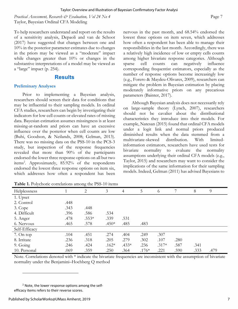
Prior to implementing a Bayesian analysis, researchers should screen their data for conditions that may be influential to their sampling models. In ordinal CFA studies, researchers can begin by investigating their indicators for low cell counts or elevated rates of missing data. Bayesian estimation assumes missingness is at least missing-at-random and priors can have an excessive influence over the posterior when cell counts are low (Buhi, Goodson, & Neilands, 2008; Gelman, 2013). There was no missing data on the PSS-10 in the PCS-3 study, but inspection of the response frequencies revealed that more than 90% of the participants endorsed the lower three response options on all but two items2. Approximately, 85.92% of the respondents endorsed the lowest three response options on item six, which addresses how often a respondent has been
2 Note, the lower response options among the self‐
efficacy items refers to their reverse scores.
nervous in the past month, and 68.54% endorsed the lowest three options on item seven, which addresses how often a respondent has been able to manage their responsibilities in the last month. Accordingly, there was a relatively high incidence of low or empty cells counts among higher bivariate response categories. Although sparse cell counts can negatively influence corresponding frequentist estimators, especially as the number of response options become increasingly low (e.g., Forero & Maydeu-Olivares, 2009), researchers can mitigate the problem in Bayesian estimation by placing moderately informative priors on any precarious parameters (Bainter, 2017).
Although Bayesian analysis does not necessarily rely on large-sample theory (Lynch, 2007), researchers should not be cavalier about the distributional characteristics they introduce into their models. For example, Natesan (2015) found that ordinal CFA models under a logit link and normal priors produced diminished results when the data stemmed from a multivariate-skewed distribution. With limited-information estimators, researchers have used tests for bivariate normality to evaluate the normality assumptions underlying their ordinal CFA models (e.g., Taylor, 2015) and researchers may want to consider the implications of the same information for their sampling models. Indeed, Gelman (2011) has advised Bayesians to
Table 1. Polychoric correlations among the PSS-10 items
Helplessness 1 2 3 4 5 6 7 8 9 1. Upset
2. Control .448
3. Cope .343 .448
4. Difficult .396 .586 .534
5. Anger .478 .553* .339 .531
6. Nervous .465 .578 .450* .485 .483
Self-Efficacy 7. On top .104 .451 .274 .404 .249 .307
8. Irritate .236 .318 .205 .279 .302 .107 .280 9. Going .246 .424 .162* .433* .236 .317* .587 .341 10. Personal .069 .359 .250 .364 .176* .221 .590 .333 .479 Note. Correlations denoted with * indicate the bivariate frequencies are inconsistent with the assumption of bivariate normality under the Benjamini–Hochberg Q method
7
Taylor: Overview and Illustration of Bayesian Confirmatory Factor Analysi
Published by ScholarWorks@UMass Amherst, 2019
Practical Assessment, Research & Evaluation, Vol 24 No 4 Page 8 Taylor, Bayesian Ordinal CFA Modeling consider the diagnostic tools available to them across estimation families. In the present study, the likelihood ratio test and the root mean square error of approximation (RMSEA), as implemented in LISREL 9.20 (Jöreskog & Sörbom, 2015), were used to identify whether one or more associations among the items was inconsistent with bivariate normality. Although results from the likelihood ratio test suggested that six pairs of items violated the bivariate normality assumption (see Table 1), none of RMSEA tests were significantly different from 0.100, indicating that any nonnormality is unlikely to be problematic (Jöreskog, 2005). The present study also checked for outliers, but no problematic response patterns were observed. Consequently, the results here suggest further that the probit link may be a reasonable choice in this study.
Bayesian Diagnostics
Overall, the two factor model did not produce any diagnostic concerns. All parameters appear to have converged to their posterior distributions as evidenced by a high degree of agreement between the Markov chains. Specifically, all PSRF values were under 1.100, indicating that the post burn-in chains exhibited few differences (Asparouhov & Muthén, 2010b). For example, 95% of the values sampled from the posterior distribution of βUpset were between 0.505 and 0.931 for one chain and 0.503 and 0.934 for the second and both chains produced a median estimate of 0.706. Likewise, visual inspection of the trace plots revealed that the chains overlapped consistently and sampled from the same range of values over the course of the post burn-in iterations for all parameters. A sample trace plot from this analysis is exampled at the top of Figure 1. Had the chains exhibited poor mixing or sampled poorly from the posterior distribution, convergence would have been questionable (Depaoli & van de Schoot, 2017). For illustrative purposes, the bottom of Figure 1 displays a trace plot with poor convergence from an analysis of the two factor model under 250 post burn-in iterations. Although the chains appear to trend together, they exhibit little overlap and both sample from different values of the parameter space over different intervals of the iterations, indicating that convergence is questionable and that more iterations are warranted (Depaoli & van de Schoot, 2017).
The diagnostics also indicated that the relationships among the items are represented well by the two factor model. The two factor model produced a ppp of .147,
indicating the hypothesized model fits the observed data well. Recall that ppp values less than .05 are evidence that a hypothesized model fits the data poorly (Lee, 2007). Also, relatively smooth changes between adjacent frequency bars across all histograms of the post burn-in chains suggests that the posterior distributions are adequately represented and that the Bayesian parameters are approximated well by the summary statistics (Depaoli & van de Schoot, 2017). A posterior distribution from this analysis is exampled at the top of Figure 1. Had one or more histograms exhibited inconsistencies over the sampling space, then parameter estimates based upon the irregular posteriors would likely have been less than ideal (Depaoli & van de Schoot, 2017). The bottom of Figure 1 illustrates a histogram that poorly represents a posterior distribution from a Bayesian analysis of the two factor model under 250 post burn-in iterations. In light of the substantial changes in the height of adjacent frequency bars more iterations are likely needed to yield satisfactory Bayesian parameter estimates (Depaoli & van de Schoot, 2017).
Unfortunately, the diagnostics did reveal elevated levels of autocorrelation for most of the chains (> .20) with some chains exhibiting large levels of autocorrelation (>.60). Researchers have generally been encouraged to address autocorrelation rather than dismiss it (e.g., Depaoli & van de Schoot, 2017; Kruschke, 2011a). Some of the reparative approaches focus on eliminating the sources of autocorrelation, such as eliminating model misspecification (Depaoli & van de Schoot, 2017), or attenuating the autocorrelation directly by extending the chains or using only every nth iteration in order to increase the independence between the simulated draws that are used to construct the posteriors (i.e., thinning; Kruschke, 2011b). Still others have suggested evaluating whether the parameters are sensitive to the high autocorrelation or not (e.g., Baldwin & Fellingham, 2013). Although low autocorrelation is desirable, if the model does not exhibit other diagnostic concerns, then high autocorrelation may not be problematic (Depaoli & van de Schoot, 2017). Since the two factor model behaved well across other diagnostic markers (e.g., PSRF values), the parameters were inspected for sensitivity to the autocorrelation by comparing the parameters before and after thinning the chains. THIN = 20 was added under the ANALYSIS command in the Mplus syntax in order to thin to every 20th iteration (Muthén & Muthén, 1998-2015), requiring
8
Practical Assessment, Research, and Evaluation, Vol. 24 [2019], Art. 4
https://scholarworks.umass.edu/pare/vol24/iss1/4DOI: https://doi.org/10.7275/vk6g-0075
Practical Assessment, Research & Evaluation, Vol 24 No 4 Page 9 Taylor, Bayesian Ordinal CFA Modeling
the chains to run 4,000,000 iterations to accumulate the 200,000 iterations requested. Although thinning the chains eliminated the autocorrelation (see Figure 2 for an example), the conclusions drawn from the model did not change and the parameter estimates exhibited little to no changes. Consequently, the elevated levels of autocorrelation appear to be inconsequential to the model.
Sensitivity analysis. Since this factor analysis is largely testing whether the indicators are meaningful contributors to the measurement of perceived stress, the sensitivity of the posterior solutions to competing tenable priors was exampled by placing priors on the parameters that increasingly favor the null hypothesis. Specifically, the loading priors were changed to N(0, 0.25) and N(0, 0.10) in turn to evaluate the sensitivity of the two factor model to weakly informative and informative priors that increasingly favor the null (Depaoli & Clifton, 2015). Under a weakly informative prior of N(0, 0.25), little to no meaningful changes were
observed. The two factor model continued to fit the data well (ppp = .135), the substantive interpretations of the loading coefficients did not change, and the parameter estimates showed moderate changes ranging from 1.580% to 6.295%. However, the substantive conclusions of the model changed as the informativeness of the priors increasingly favored the null. Under a prior of N(0, 0.10), the model exhibited dubious fit (ppp = .036), calling into question the tenability of prior probabilities that favor the null hypothesis. Consequently, the results here suggest the substantive interpretations of the model are stable and since informative priors are expected to influence the posterior, the results also do not suggest any undue influence of the priors.
Localized strains. In addition to the Bayesian diagnostics, researchers should attempt to establish the credibility of any additional assumptions made in their models. In the present case, prior research has indicated that the PSS may exhibit one or more salient cross-
Figure 1. Trace plots of the Markov chains and posterior distributions for βUpset under 250 and 100,000 post burn-in iterations. The blue and red lines in the trace plots represent two separate Markov chains while the black line running through the length of the chains represents the median of each posterior, or the Bayesian estimate for βUpset under 250 and 100,000 post burn-in iterations.
9
Taylor: Overview and Illustration of Bayesian Confirmatory Factor Analysi
Published by ScholarWorks@UMass Amherst, 2019
Practical Assessment, Research & Evaluation, Vol 24 No 4 Page 10 Taylor, Bayesian Ordinal CFA Modeling
loadings (e.g., Smith, Rosenberg, & Haight, 2014) and Hsu, Skidmore, Li, and Thompson (2014) have warned that constraining meaningful cross-loadings to zero may produce biased loading coefficients. As suggested by Hsu et al. (2014), bias in the primary loadings was investigated by freeing all the cross-loadings with a low-variance normal prior of N(0, 0.01) in keeping with the recommendations of Asparouhov, Muthén, and Morin (2015). Under the probit link and a standardized factor model, a N(0, 0.01) places 95% of the prior’s mass on standardized estimates between -0.20 and +0.20 (Kruschke, 2014; Muthén & Asparouhov, 2012) and Muthén and Asparouhov (2012) have argued that the low variance prior may free up salient cross-loadings, keep trivial cross-loadings approximately zero, and keep the model identified. Note, freeing all cross-loadings would have been prohibited under frequentist estimation because the model would not be identified. As displayed in Table 2, the primary standardized loading estimates did not exhibit meaningful changes after freeing the cross-loadings and the cross-loadings produced trivial estimates. A sensitivity analysis also revealed that the outcomes did not change by varying the informativeness of the cross-loading priors from N(0, 0.01) to N(0, 0.10). Accordingly, the cross-loadings were not retained in the final model.
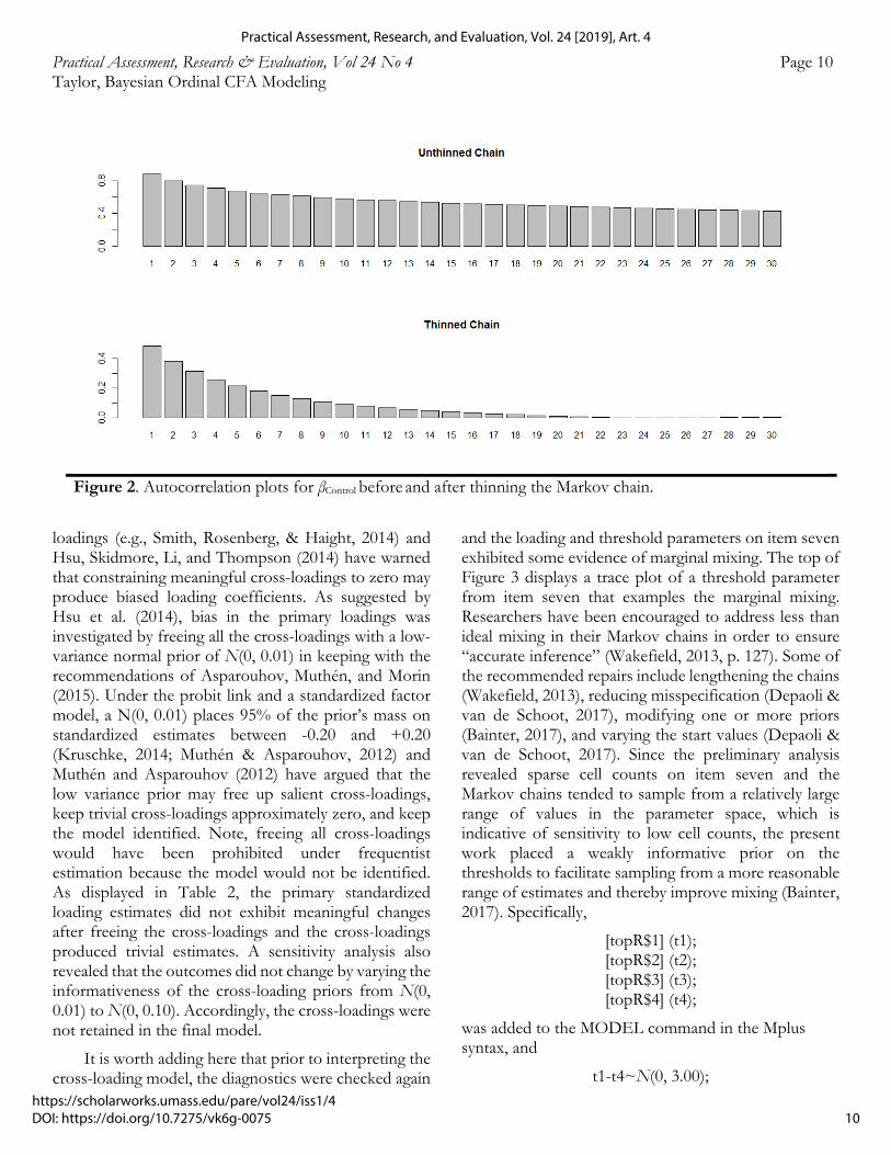
It is worth adding here that prior to interpreting the cross-loading model, the diagnostics were checked again
and the loading and threshold parameters on item seven exhibited some evidence of marginal mixing. The top of Figure 3 displays a trace plot of a threshold parameter from item seven that examples the marginal mixing. Researchers have been encouraged to address less than ideal mixing in their Markov chains in order to ensure “accurate inference” (Wakefield, 2013, p. 127). Some of the recommended repairs include lengthening the chains (Wakefield, 2013), reducing misspecification (Depaoli & van de Schoot, 2017), modifying one or more priors (Bainter, 2017), and varying the start values (Depaoli & van de Schoot, 2017). Since the preliminary analysis revealed sparse cell counts on item seven and the Markov chains tended to sample from a relatively large range of values in the parameter space, which is indicative of sensitivity to low cell counts, the present work placed a weakly informative prior on the thresholds to facilitate sampling from a more reasonable range of estimates and thereby improve mixing (Bainter, 2017). Specifically,
[topR$1] (t1); [topR$2] (t2); [topR$3] (t3); [topR$4] (t4);
was added to the MODEL command in the Mplus syntax, and
t1-t4~N(0, 3.00);
Figure 2. Autocorrelation plots for βControl before and after thinning the Markov chain.
10
Practical Assessment, Research, and Evaluation, Vol. 24 [2019], Art. 4
https://scholarworks.umass.edu/pare/vol24/iss1/4DOI: https://doi.org/10.7275/vk6g-0075
Practical Assessment, Research & Evaluation, Vol 24 No 4 Page 11 Taylor, Bayesian Ordinal CFA Modeling
was added to the MODEL PRIOR option3. Notably, the weakly informative threshold priors reduced the tendency for the Markov chains to sample from relatively extreme values in the parameter space and improved mixing, including for the loading coefficient. The bottom of Figure 3 displays an example of the improvement in mixing. Still, the results also indicated that the marginal mixing did not negatively impact the model. Changing the prior had a moderate impact on the parameter estimates at most, including among the threshold parameters on item seven, and produced no changes in the interpretations of the model. The cross-loading model did not exhibit any additional diagnostic concerns (e.g., ppp = .257).
Bayesian Interpretation of the Final Model. Since the two factor model performed well in this
study, the posterior solutions were substantively interpreted. As displayed in Table 2, median values of the standardized posterior distributions suggests that the PSS-10 items tend to load relatively well onto their respective latent factors. Standardized loading estimates
3 Although N(0, 3.00) is in keeping with the wide range of
threshold estimates researchers may encounter in their models
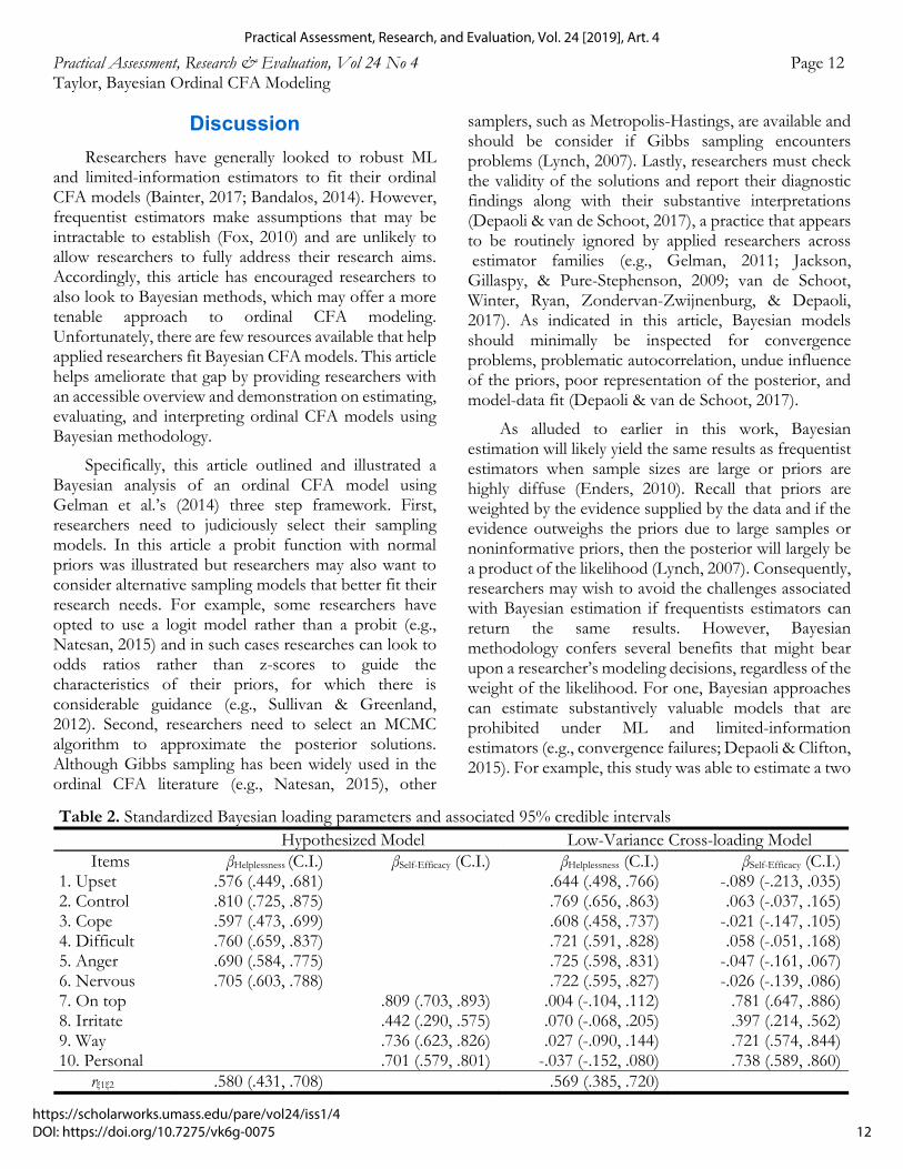
ranged from 0.576 to 0.810 among the perceived helplessness items while estimates ranged from 0.442 to 0.809 among the items assessing perceived self-efficacy. Moreover, none the 95% credible intervals (C.I.) included zero, indicating that all items credibly load onto their latent factor – the 95% C.I. denotes the interval over the parameter space where 95% of the posterior simulated estimates lie and had a 95% C.I. included zero it would have suggested that the null hypothesis was credible for the corresponding loading (Kruschke, 2013; Lynch, 2007). Item eight however, addressing a respondent’s recent experience with irritants, indicates there is a 95% chance that the true value lies between 0.290 and 0.575. Since the interval provides some evidence that a trivial loading is credible (e.g., < .32; Tabachnick & Fidell, 2013), it calls into question the substantial contribution of the item eight. Lastly, a moderate association of .580, 95% C.I. [431, .708], between the latent factors indicates that the subscales likely address distinct aspects of a respondent’s perceived stress.
(e.g., Rhemtulla et al., 2012), a range of weakly informative threshold priors were evaluated.
Figure 3. The top trace plot displays marginal mixing for the threshold capturing the step between Never and Almost never on item seven. The bottom trace plot displays the mixing of the Markov chains for the same threshold with a N(0, 3.00) prior.
11
Taylor: Overview and Illustration of Bayesian Confirmatory Factor Analysi
Published by ScholarWorks@UMass Amherst, 2019
Practical Assessment, Research & Evaluation, Vol 24 No 4 Page 12 Taylor, Bayesian Ordinal CFA Modeling
Discussion
Researchers have generally looked to robust ML and limited-information estimators to fit their ordinal CFA models (Bainter, 2017; Bandalos, 2014). However, frequentist estimators make assumptions that may be intractable to establish (Fox, 2010) and are unlikely to allow researchers to fully address their research aims. Accordingly, this article has encouraged researchers to also look to Bayesian methods, which may offer a more tenable approach to ordinal CFA modeling. Unfortunately, there are few resources available that help applied researchers fit Bayesian CFA models. This article helps ameliorate that gap by providing researchers with an accessible overview and demonstration on estimating, evaluating, and interpreting ordinal CFA models using Bayesian methodology.
Specifically, this article outlined and illustrated a Bayesian analysis of an ordinal CFA model using Gelman et al.’s (2014) three step framework. First, researchers need to judiciously select their sampling models. In this article a probit function with normal priors was illustrated but researchers may also want to consider alternative sampling models that better fit their research needs. For example, some researchers have opted to use a logit model rather than a probit (e.g., Natesan, 2015) and in such cases researches can look to odds ratios rather than z-scores to guide the characteristics of their priors, for which there is considerable guidance (e.g., Sullivan & Greenland, 2012). Second, researchers need to select an MCMC algorithm to approximate the posterior solutions. Although Gibbs sampling has been widely used in the ordinal CFA literature (e.g., Natesan, 2015), other
samplers, such as Metropolis-Hastings, are available and should be consider if Gibbs sampling encounters problems (Lynch, 2007). Lastly, researchers must check the validity of the solutions and report their diagnostic findings along with their substantive interpretations (Depaoli & van de Schoot, 2017), a practice that appears to be routinely ignored by applied researchers across estimator families (e.g., Gelman, 2011; Jackson, Gillaspy, & Pure-Stephenson, 2009; van de Schoot, Winter, Ryan, Zondervan-Zwijnenburg, & Depaoli, 2017). As indicated in this article, Bayesian models should minimally be inspected for convergence problems, problematic autocorrelation, undue influence of the priors, poor representation of the posterior, and model-data fit (Depaoli & van de Schoot, 2017).
As alluded to earlier in this work, Bayesian estimation will likely yield the same results as frequentist estimators when sample sizes are large or priors are highly diffuse (Enders, 2010). Recall that priors are weighted by the evidence supplied by the data and if the evidence outweighs the priors due to large samples or noninformative priors, then the posterior will largely be a product of the likelihood (Lynch, 2007). Consequently, researchers may wish to avoid the challenges associated with Bayesian estimation if frequentists estimators can return the same results. However, Bayesian methodology confers several benefits that might bear upon a researcher’s modeling decisions, regardless of the weight of the likelihood. For one, Bayesian approaches can estimate substantively valuable models that are prohibited under ML and limited-information estimators (e.g., convergence failures; Depaoli & Clifton, 2015). For example, this study was able to estimate a two
Table 2. Standardized Bayesian loading parameters and associated 95% credible intervals Hypothesized Model Low-Variance Cross-loading Model Items βHelplessness (C.I.) βSelf-Efficacy (C.I.) βHelplessness (C.I.) βSelf-Efficacy (C.I.)
1. Upset .576 (.449, .681) .644 (.498, .766) -.089 (-.213, .035)2. Control .810 (.725, .875) .769 (.656, .863) .063 (-.037, .165)3. Cope .597 (.473, .699) .608 (.458, .737) -.021 (-.147, .105)4. Difficult .760 (.659, .837) .721 (.591, .828) .058 (-.051, .168)5. Anger .690 (.584, .775) .725 (.598, .831) -.047 (-.161, .067)6. Nervous .705 (.603, .788) .722 (.595, .827) -.026 (-.139, .086)7. On top .809 (.703, .893) .004 (-.104, .112) .781 (.647, .886)8. Irritate .442 (.290, .575) .070 (-.068, .205) .397 (.214, .562)9. Way .736 (.623, .826) .027 (-.090, .144) .721 (.574, .844)10. Personal .701 (.579, .801) -.037 (-.152, .080) .738 (.589, .860)
rξ1ξ2 .580 (.431, .708) .569 (.385, .720)
12
Practical Assessment, Research, and Evaluation, Vol. 24 [2019], Art. 4
https://scholarworks.umass.edu/pare/vol24/iss1/4DOI: https://doi.org/10.7275/vk6g-0075
Practical Assessment, Research & Evaluation, Vol 24 No 4 Page 13 Taylor, Bayesian Ordinal CFA Modeling factor model with all the cross-loadings freed in order to test for bias in the primary loading coefficients (Hsu et al., 2014). The same test could not have been implemented using a frequentist estimator because the model would not have been identified. Also, Bayesian methods are capable of addressing conditions that may otherwise diminish results under a frequentist estimator, such as ameliorating the negative impact of sparse call counts (Bainter, 2017). Perhaps foremost though, Bayesian methodology allows researchers to rely less on large-sample theory compared to frequentist estimators since MCMC algorithms allow researchers to analyze the posterior distributions directly (Lynch, 2007).
Unfortunately, no article can address all the issues applied researchers may encounter while fitting their Bayesian models. For example, this work does not provide a background on Bayesian philosophy, which is very much a part of the Bayesian landscape. Readers are encouraged to look to the references used throughout this work to study Bayesian methodology further. Readers are particularly encouraged to see Gelman et al. (2014), Kruschke (2014), Lee (2007), and Lynch (2007). Also, while Bayesian estimation is a powerful approach to modeling, researchers should also be aware of its limitations. Perhaps foremost to this work, little methodological research has been conducted to guide the valid use of Bayesian analysis in ordinal CFA studies. For example, Bayesian tests for model fit remains a highly underdeveloped area in ordinal CFA modeling. Only the ppp has been widely adopted and it remains unclear how well it performs across increasingly diverse models (e.g., CFA models with mixed item formats). Accordingly, researchers need to be aware that practice recommendations are likely to continue to evolve as more simulation and applied works emerge.
Conclusion
Educational and psychological scientists tend to receive little training in Bayesian statistics (e.g., Aiken, West, & Millsap, 2008) and there is a paucity of resources available to help researchers capitalize on the benefits of Bayesian methodology in their CFA studies. This gap has been improving somewhat with the introduction of Bayesian estimation in common SEM software and an increase in Bayesian texts that provide thorough instruction and practice recommendations (e.g., Depaoli & van de Schoot, 2017; Lee, 2007). Still, more resources and applied examples are needed and this article helps speak to that need by focusing on the use of Bayesian
methodology in ordinal CFA studies. Foremost, this article provides readers with an example that illustrates essential Bayesian concepts and demonstrates the framework researchers should follow to fit their own ordinal models. Lastly, while this work encourages researchers to capitalize on the advantages of Bayesian methodology, readers are also advised to thoroughly address the validity of their Bayesian models.
References
Aiken, L. S., West, S. G., & Millsap, R. E. (2008). Doctoral training in statistics, measurement, and methodology in psychology: replication and extension of Aiken, West, Sechrest, and Reno's (1990) survey of PhD programs in North America. American Psychologist, 63, 32-50.
Alvarez, I., Niemi, J., & Simpson, M. (2014). Bayesian inference for a covariance matrix. In W. Song (Ed.), Proceedings of 26th Annual Conference on Applied Statistics in Agriculture (pp. 71-82). Manhattan, KS: Annual Conference on Applied Statistics in Agriculture.
Asparouhov, T., Muthén, B., & Morin, A. J. (2015). Bayesian structural equation modeling with cross-loadings and residual covariances: Comments on Stromeyer et al. Journal of Management, 20, 1-17.
Asparouhov, T., & Muthén, B. (2010a, September 29). Bayesian analysis of latent variable models using Mplus (Version 4). Retrieved from www.statmodel.com/download/BayesAdvantages18.pdf .
Asparouhov, T., & Muthén, B. (2010b, September 29). Bayesian analysis of latent variable models using Mplus: Technical implementation (Version 3). Retrieved from https:// www.statmodel.com/download/Bayes3.pdf .
Arbuckle, J. L. (2017). Amos (Version 25.0) [Computer Program]. Chicago, IL: IBM SPSS.
Baldwin, S. A., & Fellingham, G. W. (2013). Bayesian methods for the analysis of small sample multilevel data with a complex variance structure. Psychological Methods, 18, 151-164.
Bandalos, D. L. (2014). Relative performance of categorical diagonally weighted least squares and robust maximum likelihood estimation. Structural Equation Modeling: A multidisciplinary Journal, 21, 102-116.
Bainter, S. A. (2017). Bayesian estimation for item factor analysis models with sparse categorical indicators. Multivariate Behavioral Research, 52, 593-615.
Beauducel, A., & Herzberg, P. Y. (2006). On the performance of maximum likelihood versus means and
13
Taylor: Overview and Illustration of Bayesian Confirmatory Factor Analysi
Published by ScholarWorks@UMass Amherst, 2019
Practical Assessment, Research & Evaluation, Vol 24 No 4 Page 14 Taylor, Bayesian Ordinal CFA Modeling
variance adjusted weighted least squares estimation in CFA. Structural Equation Modeling: A Multidisciplinary Journal, 13, 186-203.
Berger, J. (2006). The case for objective Bayesian analysis. Bayesian Analysis, 1, 385-402.
Brown, T. A. (2015). Confirmatory factor analysis for applied research (2nd ed.). New York, NY: Guilford Press.
Bryant, F. B., & Satorra, A. (2012). Principles and practice of scaled difference chi-square testing. Structural Equation Modeling: A Multidisciplinary Journal, 19, 372-398.
Buhi, E. R., Goodson, P., & Neilands, T. B. (2008). Out of sight, not out of mind: Strategies for handling missing data. American Journal of Health Behavior, 32, 83-92.
Cohen, S., Kamarck, T., & Mermelstein, R. (1983). A global measure of perceived stress. Journal of Health and Social Behavior, 24, 385-396.
Depaoli, S., & Clifton, J. P. (2015). A Bayesian approach to multilevel structural equation modeling with continuous and dichotomous outcomes. Structural Equation Modeling: A Multidisciplinary Journal, 22, 327-351.
Depaoli, S., & van de Schoot, R. (2017). Improving transparency and replication in Bayesian statistics: The WAMBS-Checklist. Psychological Methods, 22, 240-261.
Dienes, Z. (2011). Bayesian versus orthodox statistics: Which side are you on? Perspectives on Psychological Science, 6, 274-290.
DiStefano, C. (2002). The impact of categorization with confirmatory factor analysis. Structural Equation Modeling, 9, 327-346.
DiStefano, C., & Morgan, G. B. (2014). A Comparison of diagonal weighted least squares robust estimation techniques for ordinal data. Structural Equation Modeling: A multidisciplinary Journal, 21, 425-438.
Enders, C. K. (2010). Applied missing data analysis. New York, NY: Guilford Press.
Flora, D. B., & Curran, P. J. (2004). An empirical evaluation of alternative methods of estimation for confirmatory factor analysis with ordinal data. Psychological Methods, 9, 466-491.
Forero, C. G., & Maydeu-Olivares, A. (2009). Estimation of IRT graded response models: Limited versus full information methods. Psychological Methods, 14, 275-299.
Fox, J. P. (2010). Bayesian item response modeling: Theory and applications. New York, NY: Springer Science & Business Media.
Gelman, A. (2008). Objections to Bayesian statistics. Bayesian Analysis, 3, 445-449.
Gelman, A. (2011). Induction and deduction in Bayesian data analysis. RMM, 2, 67-78.
Gelman, A. (2013, November 21). Hidden dangers of noninformative priors [Blog post]. Retrieved from http://andrewgelman.com/2013/11/21/hidden-dangers-noninformativepriors/ .
Gelman, A., Stern, H. S., Carlin, J. B., Dunson, D. B., Vehtari, A., & Rubin, D. B. (2014). Bayesian data analysis. Boca Raton, FL: Chapman and Hall/CRC.
Holgado-Tello, F. P., Chacón–Moscoso, S., Barbero–García, I., & Vila–Abad, E. (2010). Polychoric versus Pearson correlations in exploratory and confirmatory factor analysis of ordinal variables. Quality & Quantity, 44, 153-166.
Hsu, H. Y., Skidmore, S. T., Li, Y., & Thompson, B. (2014). Forced zero cross-loading misspecifications in easurement component of structural equation models: Beware of even “small” misspecifications. Methodology: European Journal of Research Methods for the Behavioral and Social Sciences, 10, 138-152.
Jackson, D. L., Gillaspy, J. A., & Purc-Stephenson, R. (2009). Reporting practices in confirmatory factor analysis: an overview and some recommendations. Psychological Methods, 14, 6-23.
Jöreskog, K. G. (2005, February 10). Structural equation modeling with ordinal variables using LISREL. Skokie, IL: Scientific Software International, Inc.
Jöreskog, K.G., & Sörbom, D. (2015). LISREL 9.20 for Windows [Computer software]. Skokie, IL: Scientific Software International, Inc.
Jöreskog, K. G., & Moustaki, I. (2001). Factor analysis of ordinal variables: A comparison of three approaches. Multivariate Behavioral Research, 36, 347-387.
Kaplan, D., & Depaoli, S. (2012). Bayesian structural equation modeling. In R. Hoyle (Ed.), Handbook of structural equation modeling (650-673). New York, NY: Guilford Press.
Kruschke, J. K. (2011a, October 5). If chains are converged, is autocorrelation okay? [Blog post]. Retrieved from http://doingbayesiandataanalysis.blogspot.com/2011/10/if-chains-are-converged-is.html.
14
Practical Assessment, Research, and Evaluation, Vol. 24 [2019], Art. 4
https://scholarworks.umass.edu/pare/vol24/iss1/4DOI: https://doi.org/10.7275/vk6g-0075
Practical Assessment, Research & Evaluation, Vol 24 No 4 Page 15 Taylor, Bayesian Ordinal CFA Modeling Kruschke, J. K. (2011b, November 5). Thinning to reduce
autocorrelation: Rarely useful. [Blog post]. Retrieved from http://doingbayesiandataanalysis.blogspot.com/2011/11/thinning-to-reduce-autocorrelation.html .
Kruschke, J. K. (2013). Bayesian estimation supersedes the t test. Journal of Experimental Psychology: General, 142, 573-603.
Kruschke, J. K. (2014). Doing Bayesian data analysis: A tutorial with R, JAGS, and Stan (2nd ed.). Burlington, MA: Academic Press.
Laboratory for the Study of Stress, Immunity, and Disease. (2016). Common Cold Project. Retrieved from http://www.commoncoldproject.com .
Lawson, A. B. (2013). Bayesian disease mapping: hierarchical modeling in spatial epidemiology. Boca Raton, FL: CRC press.
Lee, S. Y., Song, X. Y., & Cai, J. H. (2010). A Bayesian approach for nonlinear structural equation models with dichotomous variables using logit and probit links. Structural Equation Modeling, 17, 280-302.
Lee, S. (2007). Structural equation modeling: A Bayesian approach. New York, NY: John Wiley & Sons.
Li, C. H. (2016). Confirmatory factor analysis with ordinal data: Comparing robust maximum likelihood and diagonally weighted least squares. Behavior Research Methods, 48, 936-949.
Loehlin, J. C. (2004). Latent Variable Models: An Introduction to factor, path, and structural equation analysis. New York, NY: Lawrence Erlbaum.
Lynch, S. (2007). Introduction to applied Bayesian statistics and estimation for social scientists. New York, NY: Springer.
Natesan, P. (2015). Comparing interval estimates for small sample ordinal CFA models. Frontiers in Psychology, 6, 1-14.
Merkle, E. C., & Rosseel, Y. (2018). blavaan: Bayesian structural equation models via parameter expansion. Journal of Statistical Software, 85, 1-30.
Muthén, B. (2010, May). Bayesian analysis in Mplus: A brief introduction (Version 3). Retrieved from https://www.statmodel.com/download/IntroBayesVersion%203.pdf .
Muthén, B., & Asparouhov, T. (2012). Bayesian structural equation modeling: a more flexible representation of substantive theory. Psychological Methods, 17, 313-335.
Muthén, L. K., (2016, July 25). Mplus discussion board: CFA with Bayesian estimation [Online discussion board]. Retrieved from http://www.statmodel.com/discussion/messages/9/6256.html .
Muthén, L. K. and Muthén, B. O. (1998-2015). Mplus user’s guide (7th ed.). Los Angeles, CA: Muthén & Muthén.
Murdock, K. W., Seiler, A., Chirinos, D. A., Garcini, L. M., Acebo, S. L., Cohen, S., & Fagundes, C. P. (2018). Low childhood subjective social status and telomere length in adulthood: The role of attachment orientations. Developmental Psychobiology, 60, 340-346.
Myung, I. J. (2003). Tutorial on maximum likelihood estimation. Journal of Mathematical Psychology, 47, 90-100.
Pawitan, Y. (2001). In all likelihood: statistical modelling and inference using likelihood. London, UK: Oxford University Press.
Pullenayegum, E. M., & Thabane, L. (2009). Teaching Bayesian statistics in a health research methodology program. Journal of Statistics Education, 17, 1-16.
Roberti, J. W., Harrington, L. N., & Storch, E. A. (2006). Further psychometric support for the 10-item version of the Perceived Stress Scale. Journal of College Counseling, 9, 135-147.
Rhemtulla, M., Brosseau-Liard, P. É., & Savalei, V. (2012). When can categorical variables be treated as continuous? A comparison of robust continuous and categorical SEM estimation methods under suboptimal conditions. Psychological Methods, 17, 354-373.
Seaman, J. W., Seaman, J. W., & Stamey, J. D. (2012). Hidden dangers of specifying noninformative priors. The American Statistician, 66, 77-84.
Smith, K. J., Rosenberg, D. L., & Haight, G. T. (2014). An assessment of the psychometric properties of the Perceived Stress Scale‐10 (PSS10) with business and accounting students. Accounting Perspectives, 13, 29-59.
Song, X. Y., & Lee, S. Y. (2001). Bayesian estimation and test for factor analysis model with continuous and polytomous data in several populations. British Journal of Mathematical and Statistical Psychology, 54, 237-263.
Sullivan, S. G., & Greenland, S. (2012). Bayesian regression in SAS software. International Journal of Epidemiology, 42, 308-317.
Tabachnick, B., & Fidell, L. (2013). Using Multivariate Statistics (6th ed.). Boston, MA: Person Education.
15
Taylor: Overview and Illustration of Bayesian Confirmatory Factor Analysi
Published by ScholarWorks@UMass Amherst, 2019
Practical Assessment, Research & Evaluation, Vol 24 No 4 Page 16 Taylor, Bayesian Ordinal CFA Modeling Taylor, J. M. (2015). Psychometric analysis of the Ten-Item
Perceived Stress Scale. Psychological Assessment, 27, 90-101.
Taylor, J. (2019). Structural Validity of the Parenting Daily Hassles Intensity Scale. Stress and Health. Advanced online publication.
Taylor, J. M., & Bergin, C. A. (2019). The Parent/Caregiver Involvement Scale–Short form is a valid measure of parenting quality in high-risk families. Infant Behavior and Development, 54, 66-79.
van de Schoot, R., Winter, S. D., Ryan, O., Zondervan-Zwijnenburg, M., & Depaoli, S. (2017). A systematic review of Bayesian articles in psychology: The last 25 years. Psychological Methods, 22, 217-239.
Wagenmakers, E. J., Love, J., Marsman, M., Jamil, T., Ly, A., Verhagen, J., ... & Meerhoff, F. (2018). Bayesian inference for psychology. Part II: Example applications with JASP. Psychonomic Bulletin & Review, 25, 58-76.
Wakefield, J. (2013). Bayesian and frequentist regression methods. New York, NY: Springer Science & Business Media.
Yuan, K. H., Bentler, P. M., & Zhang, W. (2005). The effect of skewness and kurtosis on mean and covariance structure analysis: The univariate case and its multivariate implication. Sociological Methods & Research, 34, 240-258.
Yang-Wallentin, F., Jöreskog, K. G., & Luo, H. (2010). Confirmatory factor analysis of ordinal variables with misspecified models. Structural Equation Modeling: A Multidisciplinary Journal, 17, 392-423.
Acknowledgment:
The distributors of the PCS-3 data used in this study would like authors to include the follow acknowledgement (Murdock et al., 2018, p. 6):
The data used for this article were collected by the Laboratory for the Study of Stress, Immunity, and Disease at Carnegie Mellon University under the directorship of Sheldon Cohen, PhD; and were accessed via the Common Cold Project (CCP) website (www.commoncoldproject. com). CCP data are made publicly available through a grant from the National Center for Complementary and Integrative Health (AT006694); the conduct of the studies was supported by grants from the National Heart, Lung, and Blood Institute (HL65111; HL65112) and National Institute for Allergy and Infectious Diseases (R01 AI066367); secondary support was provided by a grant from the National Institutes of Health to the University of Pittsburgh Clinical and Translational Science Institute (UL1 RR024153 and UL1 RT000005); and supplemental support was provided by John D. and Catherine T. MacArthur Foundation Research Network on Socioeconomic Status & Health.
Citation:
Taylor, John M. (2019). Overview and Illustration of Bayesian Confirmatory Factor Analysis with Ordinal Indicators. Practical Assessment, Research & Evaluation, 24(4). Available online: http://pareonline.net/getvn.asp?v=24&n=4
Corresponding Author
John M. Taylor Saint Louis University 3525 Caroline Street, St. Louis, MO, 63104 email: johntaylor [at] slu.edu
16
Practical Assessment, Research, and Evaluation, Vol. 24 [2019], Art. 4
https://scholarworks.umass.edu/pare/vol24/iss1/4DOI: https://doi.org/10.7275/vk6g-0075

Practical Assessment, Research & Evaluation, Vol 24 No 4 Page 17 Taylor, Bayesian Ordinal CFA Modeling
Appendix A
Comments are provided after the !s to provide some instruction on the syntax. However, researchers are advised to also view A Summary of the Mplus Language found at https://www.statmodel.com/language.html for a more thorough understanding of the syntax presented here:
TITLE: Ordinal CFA with Bayesian Estimation DATA:
FILE IS = ; !Location of the data file is specified here. VARIABLE: !Users must name the columns of data in their file. NAMES ARE upset control cope difficult outside nerv topR irritateR goingR confidentR; !Variable listed after CATEGORICAL ARE are treat as ordinal variables. CATEGORICAL ARE upset control cope difficult outside nerv topR irritateR goingR confidentR; ANALYSIS:
ESTIMATOR = BAYES; !Must specify BAYES here to run Bayesian estimation. FBITERATION=200000; !Indicates the number of MCMC iterations to be used. POINT=MEDIAN; !Statistic used to as point estimate for the posterior distributions. PROCESSORS=2; !Specifies the number of MCMC chains to run.
ALGORITHM = GIBBS(PX1); !Specifies the type of MCMC algorithm to be used. BSEED = 3; !Random seed to start the MCMC chains. MODEL:
Helpless BY upset* control cope difficult outside nerv (b1 b2 b3 b4); !text in parentheses are parameter labels.
F1@1; !Standardizing the model places priors on the z-score scale. Efficacy BY topR* irritateR goingR confidentR (b6 b7 b8 b9 b10); F2@1; F1 WITH F2 (cov1);
MODEL PRIORS: b1-b10~N(0, 1);
cov1 ~IW(1, 3); OUTPUT:
STANDARDIZED; TECH8; !Will display the potential scale reduction factor.
PLOT: TYPE=PLOT3; !Supplies the posterior histograms, trace and autocorrelation plots.
17
Taylor: Overview and Illustration of Bayesian Confirmatory Factor Analysi
Published by ScholarWorks@UMass Amherst, 2019
Practical Assessment, Research & Evaluation, Vol 24 No 4 Page 18 Taylor, Bayesian Ordinal CFA Modeling
Appendix B
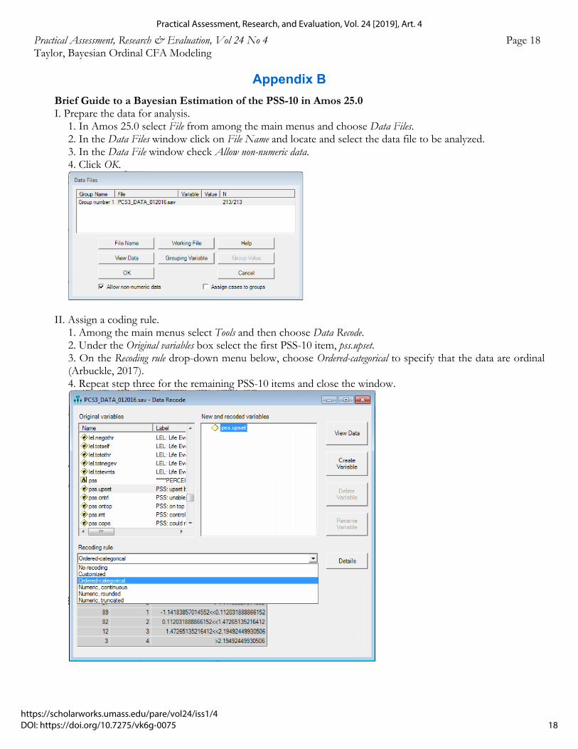
Brief Guide to a Bayesian Estimation of the PSS-10 in Amos 25.0 I. Prepare the data for analysis.
1. In Amos 25.0 select File from among the main menus and choose Data Files. 2. In the Data Files window click on File Name and locate and select the data file to be analyzed. 3. In the Data File window check Allow non-numeric data. 4. Click OK.
II. Assign a coding rule. 1. Among the main menus select Tools and then choose Data Recode.
2. Under the Original variables box select the first PSS-10 item, pss.upset. 3. On the Recoding rule drop-down menu below, choose Ordered-categorical to specify that the data are ordinal (Arbuckle, 2017). 4. Repeat step three for the remaining PSS-10 items and close the window.
18
Practical Assessment, Research, and Evaluation, Vol. 24 [2019], Art. 4
https://scholarworks.umass.edu/pare/vol24/iss1/4DOI: https://doi.org/10.7275/vk6g-0075
Practical Assessment, Research & Evaluation, Vol 24 No 4 Page 19 Taylor, Bayesian Ordinal CFA Modeling
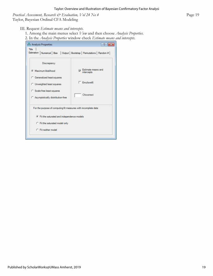
III. Request Estimate means and intercepts. 1. Among the main menus select View and then choose Analysis Properties. 2. In the Analysis Properties window check Estimate means and intercepts.
19
Taylor: Overview and Illustration of Bayesian Confirmatory Factor Analysi
Published by ScholarWorks@UMass Amherst, 2019
Practical Assessment, Research & Evaluation, Vol 24 No 4 Page 20 Taylor, Bayesian Ordinal CFA Modeling
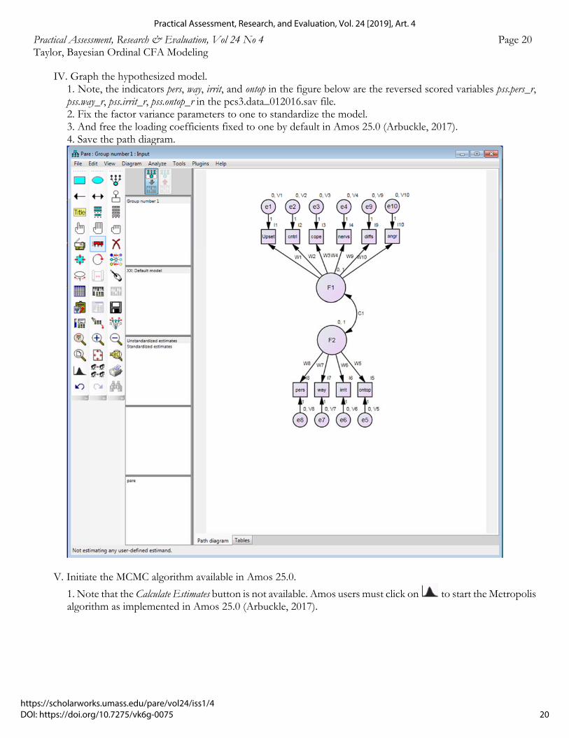
IV. Graph the hypothesized model. 1. Note, the indicators pers, way, irrit, and ontop in the figure below are the reversed scored variables pss.pers_r, pss.way_r, pss.irrit_r, pss.ontop_r in the pcs3.data_012016.sav file.
2. Fix the factor variance parameters to one to standardize the model. 3. And free the loading coefficients fixed to one by default in Amos 25.0 (Arbuckle, 2017). 4. Save the path diagram.
V. Initiate the MCMC algorithm available in Amos 25.0.
1. Note that the Calculate Estimates button is not available. Amos users must click on to start the Metropolis algorithm as implemented in Amos 25.0 (Arbuckle, 2017).
20
Practical Assessment, Research, and Evaluation, Vol. 24 [2019], Art. 4
https://scholarworks.umass.edu/pare/vol24/iss1/4DOI: https://doi.org/10.7275/vk6g-0075
Practical Assessment, Research & Evaluation, Vol 24 No 4 Page 21 Taylor, Bayesian Ordinal CFA Modeling
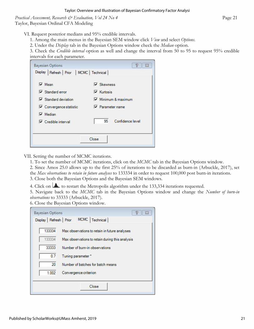
VI. Request posterior medians and 95% credible intervals. 1. Among the main menus in the Bayesian SEM window click View and select Options. 2. Under the Display tab in the Bayesian Options window check the Median option.
3. Check the Credible interval option as well and change the interval from 50 to 95 to request 95% credible intervals for each parameter.
VII. Setting the number of MCMC iterations. 1. To set the number of MCMC iterations, click on the MCMC tab in the Bayesian Options window.
2. Since Amos 25.0 allows up to the first 25% of iterations to be discarded as burn-in (Arbuckle, 2017), set the Max observations to retain in future analyses to 133334 in order to request 100,000 post burn-in iterations.
3. Close both the Bayesian Options and the Bayesian SEM windows.
4. Click on to restart the Metropolis algorithm under the 133,334 iterations requested. 5. Navigate back to the MCMC tab in the Bayesian Options window and change the Number of burn-in observations to 33333 (Arbuckle, 2017). 6. Close the Bayesian Options window.
21
Taylor: Overview and Illustration of Bayesian Confirmatory Factor Analysi
Published by ScholarWorks@UMass Amherst, 2019
Practical Assessment, Research & Evaluation, Vol 24 No 4 Page 22 Taylor, Bayesian Ordinal CFA Modeling
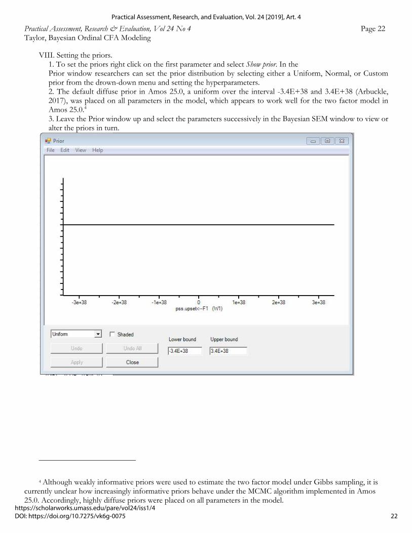
VIII. Setting the priors. 1. To set the priors right click on the first parameter and select Show prior. In the
Prior window researchers can set the prior distribution by selecting either a Uniform, Normal, or Custom prior from the drown-down menu and setting the hyperparameters. 2. The default diffuse prior in Amos 25.0, a uniform over the interval -3.4E+38 and 3.4E+38 (Arbuckle, 2017), was placed on all parameters in the model, which appears to work well for the two factor model in Amos 25.0.4 3. Leave the Prior window up and select the parameters successively in the Bayesian SEM window to view or alter the priors in turn.
4 Although weakly informative priors were used to estimate the two factor model under Gibbs sampling, it is currently unclear how increasingly informative priors behave under the MCMC algorithm implemented in Amos 25.0. Accordingly, highly diffuse priors were placed on all parameters in the model.
22
Practical Assessment, Research, and Evaluation, Vol. 24 [2019], Art. 4
https://scholarworks.umass.edu/pare/vol24/iss1/4DOI: https://doi.org/10.7275/vk6g-0075
Practical Assessment, Research & Evaluation, Vol 24 No 4 Page 23 Taylor, Bayesian Ordinal CFA Modeling
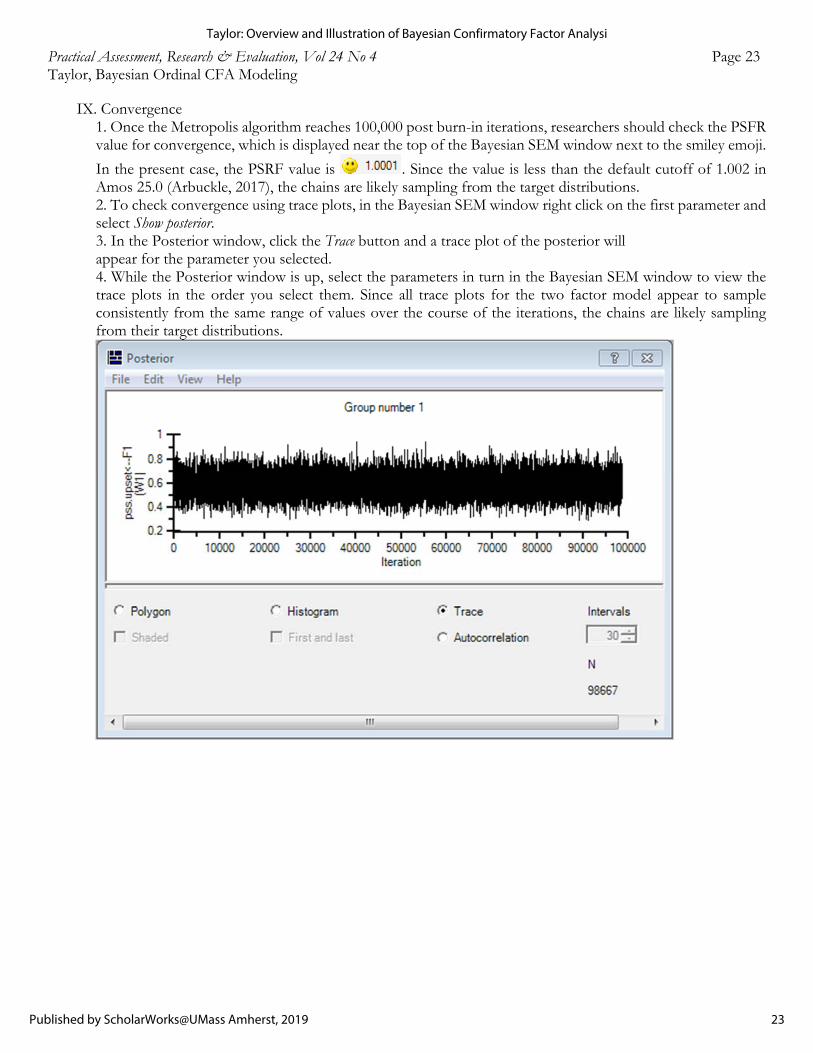
IX. Convergence 1. Once the Metropolis algorithm reaches 100,000 post burn-in iterations, researchers should check the PSFR value for convergence, which is displayed near the top of the Bayesian SEM window next to the smiley emoji.
In the present case, the PSRF value is . Since the value is less than the default cutoff of 1.002 in Amos 25.0 (Arbuckle, 2017), the chains are likely sampling from the target distributions. 2. To check convergence using trace plots, in the Bayesian SEM window right click on the first parameter and select Show posterior. 3. In the Posterior window, click the Trace button and a trace plot of the posterior will
appear for the parameter you selected. 4. While the Posterior window is up, select the parameters in turn in the Bayesian SEM window to view the trace plots in the order you select them. Since all trace plots for the two factor model appear to sample consistently from the same range of values over the course of the iterations, the chains are likely sampling from their target distributions.
23
Taylor: Overview and Illustration of Bayesian Confirmatory Factor Analysi
Published by ScholarWorks@UMass Amherst, 2019
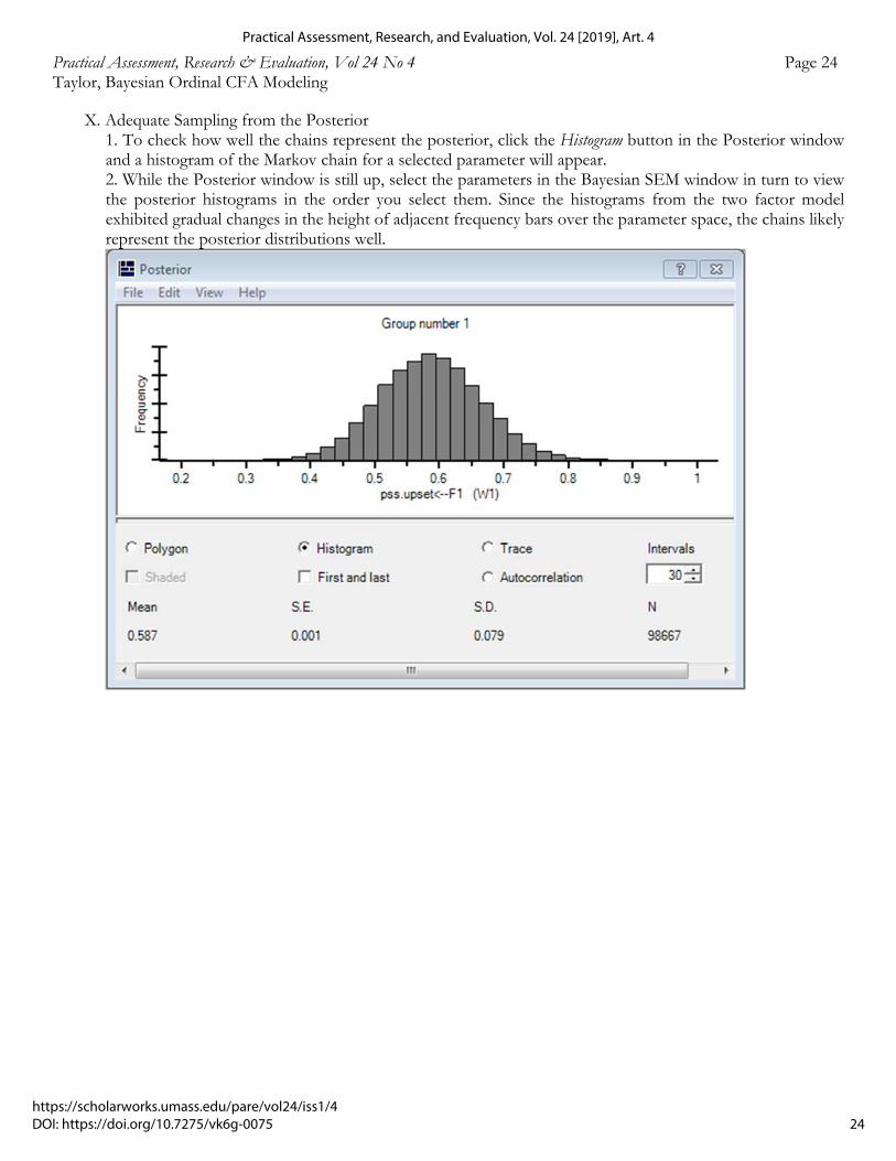
Practical Assessment, Research & Evaluation, Vol 24 No 4 Page 24 Taylor, Bayesian Ordinal CFA Modeling
X. Adequate Sampling from the Posterior 1. To check how well the chains represent the posterior, click the Histogram button in the Posterior window and a histogram of the Markov chain for a selected parameter will appear. 2. While the Posterior window is still up, select the parameters in the Bayesian SEM window in turn to view the posterior histograms in the order you select them. Since the histograms from the two factor model exhibited gradual changes in the height of adjacent frequency bars over the parameter space, the chains likely represent the posterior distributions well.
24
Practical Assessment, Research, and Evaluation, Vol. 24 [2019], Art. 4
https://scholarworks.umass.edu/pare/vol24/iss1/4DOI: https://doi.org/10.7275/vk6g-0075
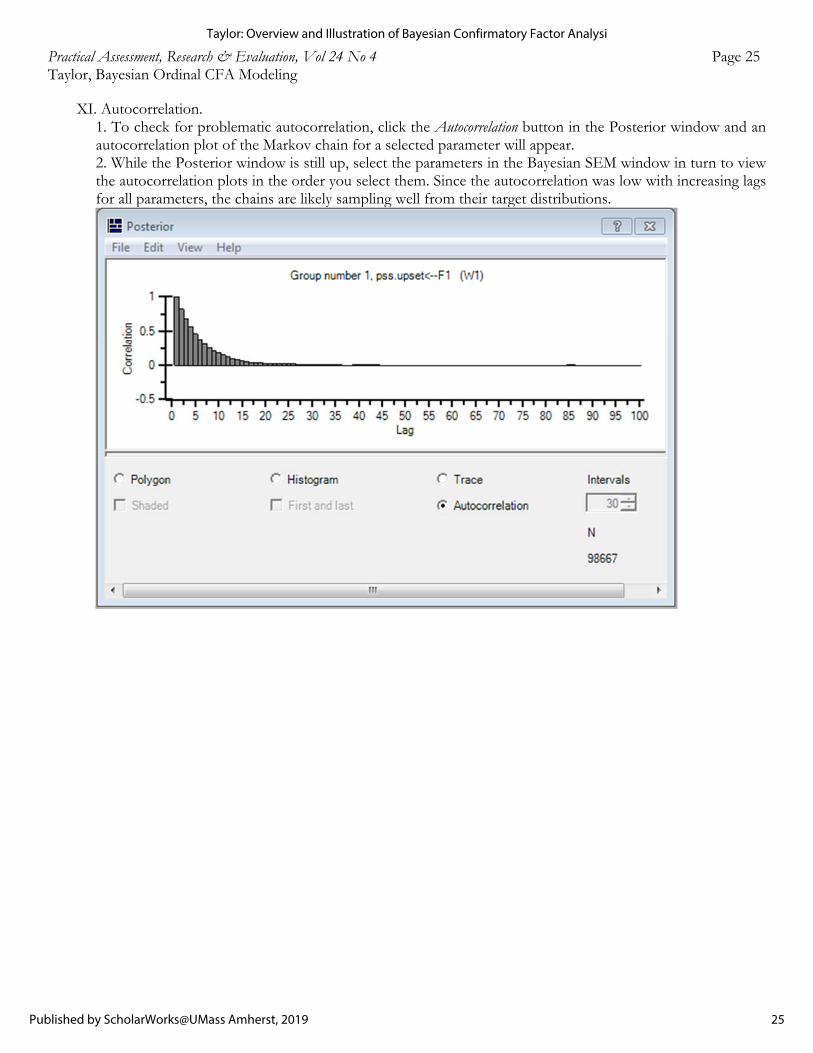
Practical Assessment, Research & Evaluation, Vol 24 No 4 Page 25 Taylor, Bayesian Ordinal CFA Modeling
XI. Autocorrelation. 1. To check for problematic autocorrelation, click the Autocorrelation button in the Posterior window and an autocorrelation plot of the Markov chain for a selected parameter will appear. 2. While the Posterior window is still up, select the parameters in the Bayesian SEM window in turn to view the autocorrelation plots in the order you select them. Since the autocorrelation was low with increasing lags for all parameters, the chains are likely sampling well from their target distributions.
25
Taylor: Overview and Illustration of Bayesian Confirmatory Factor Analysi
Published by ScholarWorks@UMass Amherst, 2019
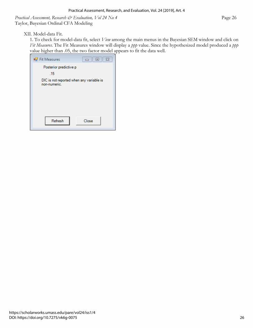
Practical Assessment, Research & Evaluation, Vol 24 No 4 Page 26 Taylor, Bayesian Ordinal CFA Modeling
XII. Model-data Fit. 1. To check for model-data fit, select View among the main menus in the Bayesian SEM window and click on Fit Measures. The Fit Measures window will display a ppp value. Since the hypothesized model produced a ppp value higher than .05, the two factor model appears to fit the data well.
26
Practical Assessment, Research, and Evaluation, Vol. 24 [2019], Art. 4
https://scholarworks.umass.edu/pare/vol24/iss1/4DOI: https://doi.org/10.7275/vk6g-0075
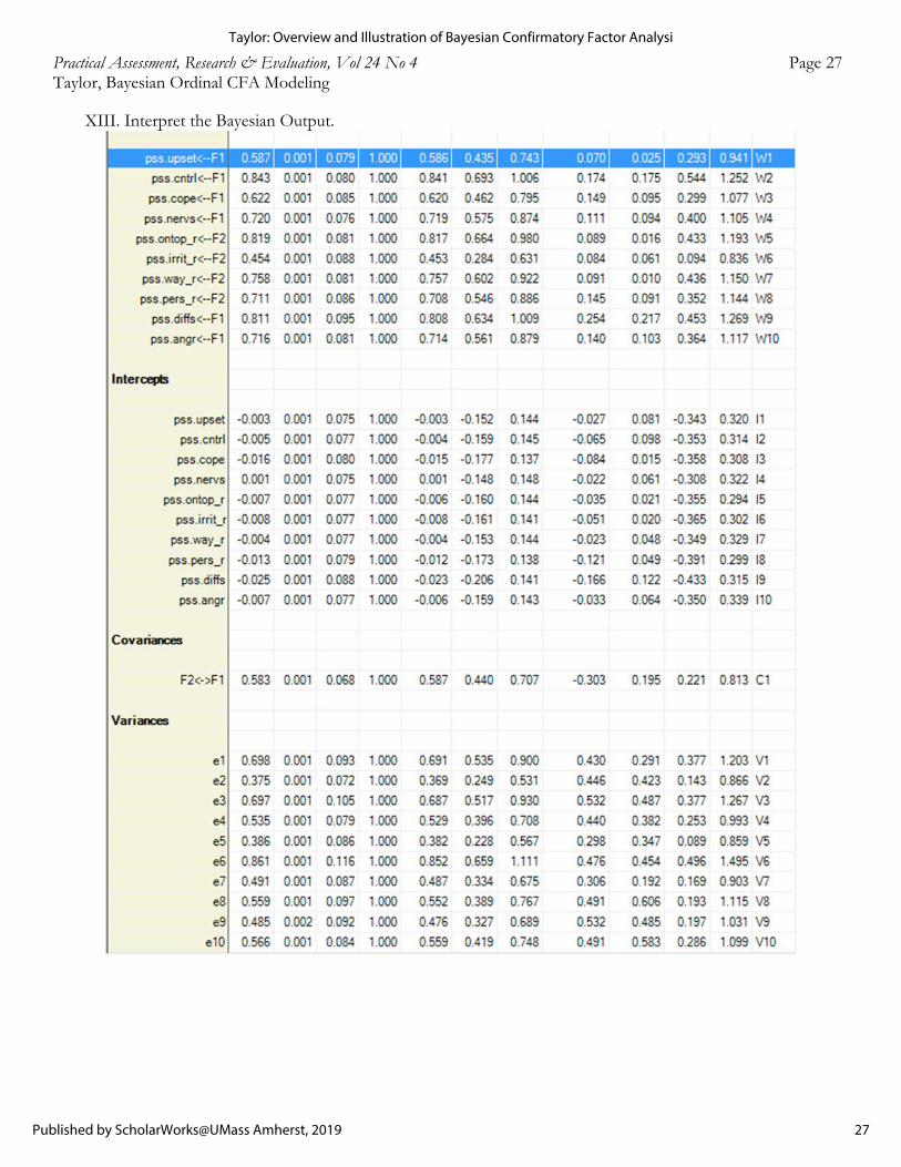
Practical Assessment, Research & Evaluation, Vol 24 No 4 Page 27 Taylor, Bayesian Ordinal CFA Modeling
XIII. Interpret the Bayesian Output.
27
Taylor: Overview and Illustration of Bayesian Confirmatory Factor Analysi
Published by ScholarWorks@UMass Amherst, 2019