Overview for Week 2 - Alex Smola for Week 2 What is Learning Theory Basic Idea, Classi cation, Regression, Novelty Detection, Applications Statistics Probabilities, Distributions,

Overview for Week 2

What is Learning Theory

Basic Idea, Classification, Regression, Novelty Detection, Applications

Statistics

Probabilities, Distributions, Bayes Rule, Measures

Useful Distributions

Normal Distribution, Laplacian Distribution, Mean, Variance

Maximum Likelihood Estimators

Parameter Adjustment, Density Estimation, Optimization Problems

Convergence

Law of Large Numbers, Curse of Dimensionality, Overfitting

Perceptron

Biological Background, Hebbian Learning, Half Spaces, Linear Functions, Perceptron

Learning Rule, Convergence Theorem, Applications, Algorithms and Extensions.

Alex Smola: ENGN 4520 - Introduction to Machine Learning, Week 2, Lecture 1, http://axiom.anu.edu.au/∼smola/engn4520/week2 l1 4.pdf Page 1

Learning Theory

Supervised Learning

We have some empirical data (images, medical observations, market indicators, so-

cioeconomical background of a person, texts), say xi ∈ X, usually together with

labels yi ∈ Y (digits, diseases, share price, credit rating, relevance) and we want to

find a function that connects x with y.

Cost of Misprediction

Typically, there will be a function c(x, y, f(x)) depending on x, y and the prediction

f (x) which tells us the loss we incur by estimating f (x) instead of the actual value

y. This may be, e.g. the number of wrong characters in an OCR application, the

cost for wrong treatment, the actual loss of money on the stock exchange, the cost

for a bankrupt client, or the amount of annoyance by receiving a wrong e-mail.

Unsupervised Learning

We have some data xi and we want to find regularities or interesting objects in

general from the data.Alex Smola: ENGN 4520 - Introduction to Machine Learning, Week 2, Lecture 1, http://axiom.anu.edu.au/∼smola/engn4520/week2 l1 4.pdf Page 2

Classification

Goal

We want to find a function f : X→ {±1} or f : X→ R which will tell us whether

a new observation x ∈ X belongs to class 1 or −1 (and possibly the confidence with

which this is so.

Questions

How to rate f , how to find f , how to interpret f (x), . . .


Applications

Optical Character Recognition

The goal is to classify (handwritten) characters (note that here f has to map into

{a, . . . , z} rather than into {−1, 1}) automatically (form readers, scanners, post).

Spam Filtering

Determine whether an e-mail is spam or not (or whether it is urgent), based on

keywords, word frequencies, special characters ($, !, uppercase, whitespace), . . .

Medical Diagnosis

Given some observations such as immune status, blood pressure, etc., determine

whether a patient will develop a certain disease. Here it matters that we can estimate

the probability of such an outcome.

Face Detection

Given a patch of an image, determine whether this corresponds to a face or not

(useful for face tracking later — see e.g. Seeing Machines).


Learning is not (only) Memorizing

Goal

Infer from a training set {(x1, y1), . . . , (xm, ym)} to the general connection between

x and y.

Simple and Dumb Learning

Memorize all the data {(x1, y1), . . . , (xm, ym)} we are given. This clearly gets the

hypotheses on the training set right (popular strategy in the 80s), but what to do

for new x?

Slightly Better Strategy

Memorize all the data and for new observations predict the same as the closest

neighbour xi to x does (Nearest Neighbour algorithm).

Problem

What about noisy and unreliable data? Different notions of proximity? We want to

generalize our training data to new and unknown concepts.


Errors in Classification

Classification Error

We say that a classification error occurs, if sgn f (x) 6= y, i.e. if sgn f (x) predicts an

outcome different from y.

Data Generation

Assume that the x are drawn from some distribution (we will come back to that

later ) and that y is either deterministic (for every x there is only one true y) or

random (y = 1 occurs in a fraction p of all cases and y = −1 in a fraction of 1− pcases).

This “distribution” could simply be due to someone writing 0 and 1 on a piece of

paper. Or the different processes that smudge and degrade paper when an envelope

ends up in the postbox.

Goal

We want to rate our classifier f with respect to this data generating process.


Performance Guarantees

Expected Error

It is the average error we can expect for new data arriving, i.e.

R[f ] = E(x,y) [sgn f (x) 6= y]

Sometimes we also call R[f ] the expected risk.

Training Error

The average error on the training set

Remp[f ] :=1

m

m∑i=1

(sgn f (xi) 6= yi)

Sometimes we also call Remp[f ] the empirical risk.

Connection between Expected Error and Training Error

How much can we say about R[f ], given Remp[f ]? Clearly R[f ] can (and usually

will) exceed the training error. We want to know the probability of this happening.


Regression

Goal

We want to find a function f : X→ R which will tell us the value of f at x.

Application: Getting Rich

Predict the stock value of IBM/CISCO/BHP/TELSTRA . . . given today’s market

indicators (plus further background data).

Application: Wafer Fab

Predict (and optimize) the yield for a microprocessor, given the process parameters

(temperature, chemicals, duration, . . . ).

Application: Network Routers

Predict the network traffic through some hubs/routers/switches. We could reconfig-

ure the infrastructure in time . . .

Application: Drug Release

Predict the requirement for a certain drug (e.g. insulin) automatically.


Example


Novelty Detection

Goal

• Build estimator that finds unusual observations and outliers

• Build estimator that can assess how typical an observation is

Idea

• Data is generated according to some density p(x). Find regions of low density.

• Such areas can be approximated as the level set of an auxiliary function. No

need to estimate p(x) directly — use proxy of p(x).

• Specifically: find f (x) such that x is novel if f (x) ≤ c where c is some constant,

i.e. f (x) describes the amount of novelty.


Applications

Network Intrusion Detection

Detect whether someone is trying to hack the network, downloading tons of MP3s,

or doing anything else unusual on the network.

Jet Engine Failure Detection

You can’t (normally) destroy a couple of jet engines just to see how they fail.

Database Cleaning

We want to find out whether someone stored bogus information in a database (typos,

etc.), mislabelled digits, ugly digits, bad photographs in an electronic album.

Fraud Detection

Credit Card Companies, Telephone Bills, Medical Records

Self calibrating alarm devices

Car alarms (adjusts itself to where the car is parked), home alarm (location of

furniture, temperature, open windows, etc.)


Probability

Basic Idea

We have events, denoted by sets X ⊂ X in a space of possible outcomes X. Then

P(X) tells us how likely is that an event x with x ∈ X will occur.

Basic Axioms

• Pr(X) ∈ [0, 1] for all X ⊆ X

• Pr(X) = 1

• Pr (∪iXi) =∑i

Pr(Xi) if Xi ∩Xj = ∅ for all i 6= j

Actually, we were a bit sloppy — P(X) may not always defined and all we need is

a σ-algebra on X. But we won’t worry about this here . . .

Simple Corollary

Pr(Xi ∪Xj) = Pr(Xi) + Pr(Xj)− Pr(Xi ∩Xj)


Multiple Variables

Two Sets

Assume we have X and Y and a probability measure on the product space of X and

Y. Then we may consider the space of events (x,y) ∈ X × Y and ask how likely

events in such a space are.

Independence

If the events x and y are independent, for any sets X ⊂ X and Y ⊂ Y we have

Pr(X, Y ) = Pr(X) · Pr(Y ).

Here Pr(X, Y ) is the probability that any (x,y) with xinX and y ∈ Y occur.

Dependence and Conditional Probability

Typically, knowing x will tell us something about y (think regression or classifica-

tion). We have

Pr(Y |X) Pr(X) = Pr(Y,X).

This implies Pr(Y,X) ≤ min(Pr(X),Pr(Y )).


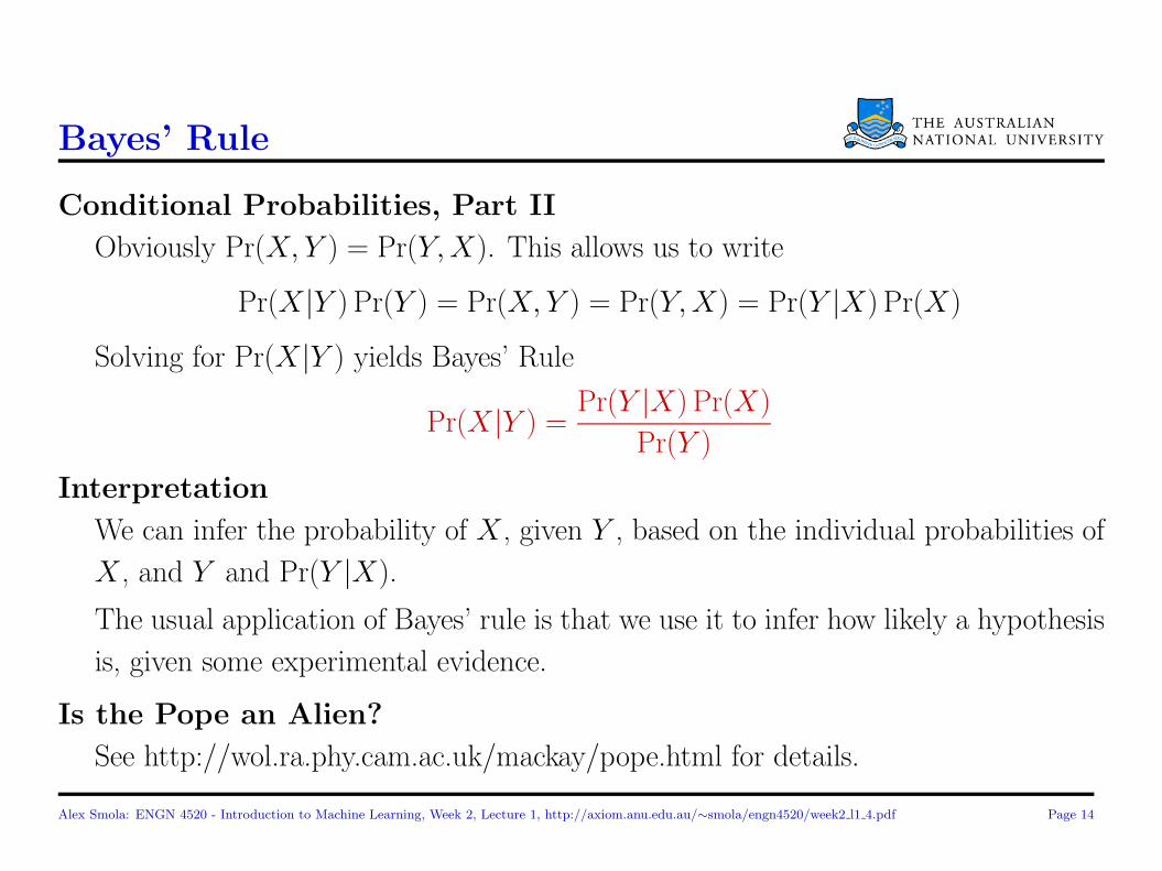
Bayes’ Rule

Conditional Probabilities, Part II

Obviously Pr(X, Y ) = Pr(Y,X). This allows us to write

Pr(X|Y ) Pr(Y ) = Pr(X, Y ) = Pr(Y,X) = Pr(Y |X) Pr(X)

Solving for Pr(X|Y ) yields Bayes’ Rule

Pr(X|Y ) =Pr(Y |X) Pr(X)

Pr(Y )

Interpretation

We can infer the probability of X , given Y , based on the individual probabilities of

X , and Y and Pr(Y |X).

The usual application of Bayes’ rule is that we use it to infer how likely a hypothesis

is, given some experimental evidence.

Is the Pope an Alien?

See http://wol.ra.phy.cam.ac.uk/mackay/pope.html for details.


Examples

AIDS-Test

We want to find out likely it is that a patient really has AIDS (denoted by X) if

the test is positive (denoted by Y ).

Roughly 0.1% of all Australians are infected (Pr(X) = 0.001). The probability that

an AIDS test tells us the wrong result is in the order of 1% (Pr(Y |X\X) = 0.01)

and moreover we assume that it detects all infections (Pr(Y |X) = 1). We have

Pr(X|Y ) =Pr(Y |X) Pr(X)

Pr(Y )=

Pr(Y |X) Pr(X)

Pr(Y |X) Pr(X) + Pr(Y |X\X) Pr(X\X)

Hence Pr(X|Y ) = 1·0.0011·0.001+0.01·0.999 = 0.091, i.e. the probability of AIDS is 9.1%!

Reliability of Eye-Witness

Assume that an eye-witness is 90% sure and that there were 20 people at the crime

scene, what is the probability that the guy identified committed the crime?

Pr(X|Y ) =0.9 · 0.05

0.9 · 0.05 + 0.1 · 0.95= 0.3213 = 32% that’s a worry . . .


Distribution, Measure, and Densities

Computing Pr(X)

Quite often X will not be a countable set, e.g., for X = R. So we need integrals.

Pr(X) :=

∫X

dPr(x) =

∫X

p(x)dx

Note that the last equality only holds if such a p(x) exists. For the rest of this course

we assume that such a p exists . . .


Bayes’ Rule for Densities

Multivariate Densities

As with conditional probabilities we can also have densities on product spaces X×Y,

given by p(x,y).

Conditional Densities

For independent variables the densities factorize and we have

p(x,y) = p(x)p(y)

For dependent variables (i.e. x tells us something about y and vice versa) we obtain

p(x,y) = p(x|y)p(y) = p(y|x)p(x)

Bayes’ Rule

Solving for p(y|x) yields

p(y|x) =p(x|y)p(y)

p(x)


Example: p(x) = 1 + sin x

Factorizing Distribution


Random Variables

Definition

If we want to denote the fact that variables x and y are drawn at random from an

underlying distribution, we call them random variables.

IID variables

This means Independent and Identically Distributed random variables. Most of our

data has this property (e.g. each face we scan is independent of the other faces we

saw). In this case the density factorizes into

p({x1, . . . ,xm}) =

m∏i=1

p(xi)

Dependent Random Variables

For prediction purposes we want to estimate y from x. In this case we want that y

is dependent on x. If p(x,y) = p(x)p(y) we could not predict at all!


Marginalization and Conditioning

Marginalization

Given p(x,y) we want to obtain p(x). For this purpose we integrate out y via

p(x) =

∫Y

p(x,y)dy

Conditioning

If we know y, we can obtain p(x|y) via Bayes rule, i.e.

p(x|y) =p(y|x)p(x)

p(y)=p(x,y)

p(y).

A simler trick, however, is to note that the dependence of the RHS on x lies only in

p(x,y) and therefore we obtain

p(x|y) =p(x,y)∫

Xp(x,y)dx


Documents

Overview for Week 2 - Alex Smola for Week 2 What is Learning Theory Basic Idea, Classi cation, Regression, Novelty Detection, Applications Statistics Probabilities, Distributions,