BackgroundBackground

Overview of

Projective Geometry

Topics Covered

Background (Projective Geometry)

Single View

Double View

Triple View

N-view

Robust parameter estimation

‘Projective’ Geometry

Study relations between different classes of coordinate transformations

Maintain Co-linearity (iff XXXX’’’’=HXHXHXHX)

Not necessarily maintain

Angle and length (Euclidean)

Angle and relative length (similarity)

Parallelism, line and plane at infinity (affine)

Intersection and tangency (projective)

Class Diagram

Note that perspective camera projection is notnotnotnot in the hierarchy

Projective geometry does not, theoretically, have to involve cameras (e.g. Euclidean)

But many concepts are very useful in camera calibration and image analysis

SimilarityEuclidean Affine Projective

Invariants

100

2221

1211

y

x

taa

taa

100

2221

1211

y

x

tsrsr

tsrsr

333231

232221

131211

hhh

hhh

hhh

100

2221

1211

y

x

trr

trr

Projective

8dof

Affine

6dof

Similarity

4dof

Euclidean

3dof

Concurrency, collinearity, order of contact (intersection, tangency, inflection, etc.), cross ratio

Parallelism, ratio of areas, ratio of lengths on parallel lines (e.g midpoints), linear combinations of vectors (centroids). The line at infinity lThe line at infinity lThe line at infinity lThe line at infinity l

∞

Ratios of lengths, angles.The circular points I,JThe circular points I,JThe circular points I,JThe circular points I,J

lengths, areas.

Transformation Hierarchy

Rectification

What information (constraint) needed to be supplied to go up in the hierarchy

Additional information limits the degrees of freedom

Rectification is a mathematic process of limiting DOFs of H H H H (camera or not)

63Euclidean

74Similarity

126Affine

158Projective

3D2D

Decomposition of projective transformations

=

==

vv

sPAS TTTT v

tA

v

IKtRHHHH

0

10

0

10

TtvRKA += s

K 1det =Kupper-triangular,

decomposition unique (if chosen s>0)

=

0.10.20.1

0.2242.8707.2

0.1586.0707.1

H

−

=

121

010

001

100

020

015.0

100

0.245cos245sin2

0.145sin245cos2oo

oo

H

Example:

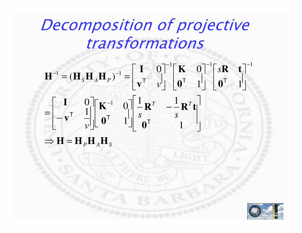
Decomposition of projective transformations

SAP

TT

PAS

ssv

s

v

HHHH

0

tRR

0

K

v

I

0

tR

0

K

v

IHHHH

=⇒

−

−=

==

−

−−−

−−

1

11

1

010

11

00)(

1

111

11

TT

T

TTT

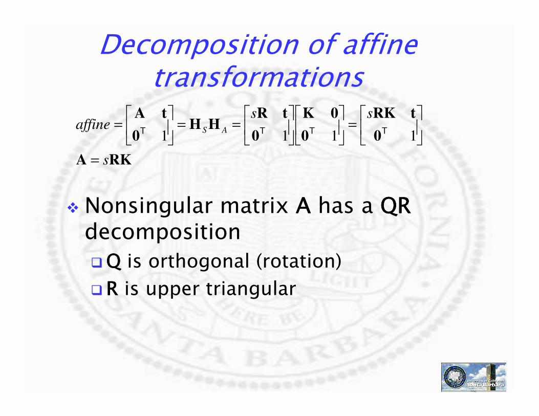
Decomposition of affine transformations

RKA

0

tRK

0

0K

0

tRHH

0

tA

s

ssaffine AS

=

=

==

=

1111 TTTT

Nonsingular matrix AAAA has a QRQRQRQRdecomposition

QQQQ is orthogonal (rotation)

RRRR is upper triangular

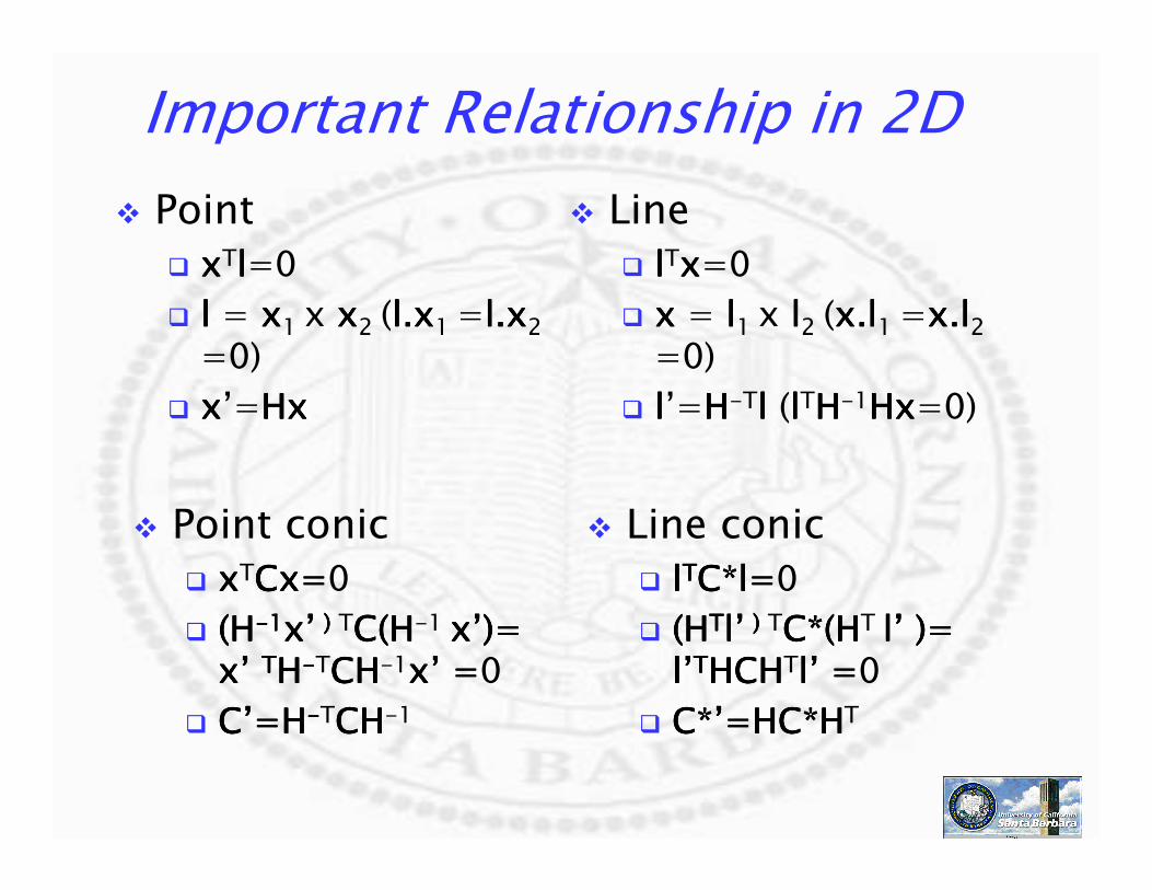
Important Relationship in 2D

Point

xxxxTllll=0

llll = xxxx1 x xxxx2 (l.l.l.l.xxxx1 =l.l.l.l.xxxx2 =0)

xxxx’=HxHxHxHx

Line

llllTxxxx=0

xxxx = llll1 x llll2 (x.x.x.x.llll1 =x.x.x.x.llll2 =0)

llll’=HHHH-Tllll (llllTHHHH-1HxHxHxHx=0)

Point conic

xxxxTCxCxCxCx====0

(H(H(H(H----1111xxxx’’’’ ) ) ) ) TC(HC(HC(HC(H-1 xxxx’’’’)= )= )= )= xxxx’’’’ TTTTHHHH----TCHCHCHCH-1xxxx’’’’ ====0

CCCC’’’’=H=H=H=H----TCHCHCHCH-1

Line conic

llllTTTTCCCC*l=*l=*l=*l=0

((((HHHHTTTTllll’’’’ ) ) ) ) TC*(HC*(HC*(HC*(HT llll’’’’ )= )= )= )= llll’’’’TTTTHCHHCHHCHHCHTllll’’’’ ====0

C*C*C*C*’’’’=HC*H=HC*H=HC*H=HC*HT

Important Relationship in 2D (cont.)

Point at infinity

(rx,ry,1) r-> infinity

(x,y,0)

(x,y,0).(0,0,1) = 0

Line at infinity

(a b).(x y) = r, r-> infinity

(0,0,1)

(0,0,1).(x,y,0) =0

Degenerate point conic

C=lmlmlmlmT+mlmlmlmlT, llllllllT

Rank two, rank one

Null space xxxx = l x ml x ml x ml x m

Degenerate line conic

C* = xyxyxyxyT + yxyxyxyxT,xxxxxxxxT

Rank two, rank one

Null space llll = x x yx x yx x yx x y

Absolute dual conic is degenerate line conics

Dual Relationship of Pole and Polar in

2D for Point and Line Conic

Point conic xxxxTTTTCxCxCxCx=0

Tangent CCCCTTTTxxxx

Pole not on the conic xxxx

Polar line CxCxCxCx

Point on polar line yyyyTTTTCxCxCxCx=0=0=0=0

Point also on conic

Pole on tangent line (CCCCTTTTy)y)y)y)TTTTxxxx=0=0=0=0

Line conic llllTTTTCCCC*l*l*l*l=0

Tangent point C*C*C*C*TTTTllll

Polar not tangent to conic llll

Pole C*lC*lC*lC*l

Line passing through pole mmmmTTTTCCCC*l=0*l=0*l=0*l=0

Line tangent to conic

Polar passing through contact (C*C*C*C*TTTTm)m)m)m)TTTTllll=0=0=0=0

x

Cx

y

C*l

l

C*Tm

m

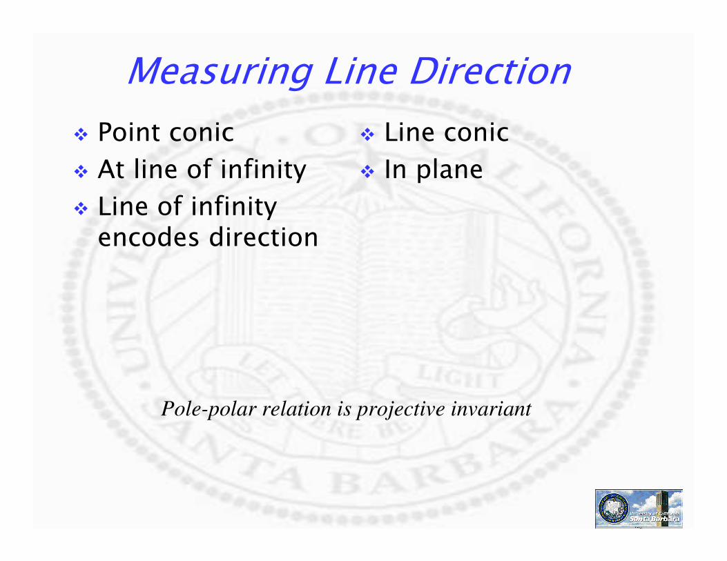
Measuring Line Direction

Point conic

At line of infinity

Line of infinity encodes direction

Line conic

In plane

Pole-polar relation is projective invariant

Dual Relationship in 2D

Circular points

On line of infinity

Dual conic

Degenerate line conic

mmmmTTTTCCCC*l=0, C*=IJ*l=0, C*=IJ*l=0, C*=IJ*l=0, C*=IJT+JI+JI+JI+JIT

Measure lineorientation

Important Relationship in 3D

Point

PPPPTXXXX=0

XXXX’’’’=HX=HX=HX=HX

Plane

XXXXTPPPP=0

PPPP’’’’ = H= H= H= H----TTTTPPPP

Point quadric

XXXXTQX=QX=QX=QX=0

(H(H(H(H----1111XXXX’’’’ ))))TQ(HQ(HQ(HQ(H----1 1 1 1 XXXX’’’’)= )= )= )= XXXX’’’’ TTTTHHHH----TQHQHQHQH----1111XXXX’’’’ ====0

QQQQ’’’’=H=H=H=H----TQHQHQHQH----1111

Plane quadric

PPPPTQ*P=Q*P=Q*P=Q*P=0

(H(H(H(HTTTTPPPP’’’’ ) ) ) ) TQ*(HQ*(HQ*(HQ*(HTPPPP’’’’ )= )= )= )= PPPP’’’’TTTTHQ*HHQ*HHQ*HHQ*HTPPPP’’’’ ====0

Q*Q*Q*Q*’’’’=HQ*H=HQ*H=HQ*H=HQ*HT

Dual Relationship of Pole and Polar in 3D for Point and Plane Quadric

Point quadric XXXXTTTTQXQXQXQX=0

Tangent plane QQQQTTTTXXXX

Pole not on the quadric XXXX

Polar plane QXQXQXQX

Point on polar plane YYYYTTTTQX=0QX=0QX=0QX=0

Point also on quadric

Pole on tangent plane (QQQQTTTTY)Y)Y)Y)TTTTX=0X=0X=0X=0

Plane quadric PPPPTTTTQ*PQ*PQ*PQ*P=0

Tangent point Q*Q*Q*Q*TTTTPPPP

Polar plane not tangent to quadric PPPP

Pole Q*PQ*PQ*PQ*P

Plane passing through pole SSSSTTTTQ*P=0Q*P=0Q*P=0Q*P=0

Plane tangent to quadric

Polar passing through contact (Q*Q*Q*Q*TTTTS)S)S)S)TTTTP=0P=0P=0P=0

Measuring Direction in 3D

Line Direction

Point conic in plane of infinity

Line conic in space

Plane direction

Plane quadric in space

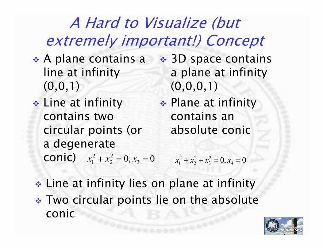
A Hard to Visualize (but extremely important!) Concept

A plane contains a line at infinity (0,0,1)

Line at infinity contains two circular points (or a degenerate conic)

3D space contains a plane at infinity (0,0,0,1)

Plane at infinity contains an absolute conic

Line at infinity lies on plane at infinity

Two circular points lie on the absolute conic

0,0 3

2

2

2

1 ==+ xxx 0,0 4

2

3

2

2

2

1 ==++ xxxx

Proof

Line at infinity lies on plane at infinity

(or point at infinity lies on plane at infinity)

Circular points lie on absolute conic

+

=

0

|

|

0

|

|

0

0

1000

|||

|||

21

3

2321

1

rrrrryx

y

x

t

t

t

0

0||2||

)()(

0

|

|

0

|

|

0

0

1

1000

|||

|||

4

2

221

2

1

2121

2

3

2

2

2

1

21

3

2321

1

=

=−⋅+=

+⋅+=++

+

=

x

i

iixxx

ii

t

t

t

rrrr

rrrr

rrrrr

A Hard to Visualize Concept

3D plane

Line at infinity

All circles intersect AC in two points (circular points)

All spheres intersect plane at infinity in AC

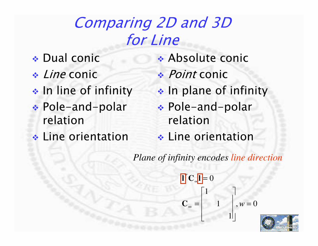
Comparing 2D and 3Dfor Line

Dual conic

Line conic

In line of infinity

Pole-and-polar relation

Line orientation

Absolute conic

Point conic

In plane of infinity

Pole-and-polar relation

Line orientation

0,

1

1

1

0

=

=

=

∞

∞

w

T

C

lCl

Plane of infinity encodes line direction

Dual Relationship in 3D

Absolute conic (AC)

On line of infinity

Backproject into ADQ

Measure lineorientation

Absolute dual quadric (ADQ)

In space

Project into ADC

Measure planeorientation

=

=

∞

∞

0

1

1

1

0

*

*

C

PCPT

0,

1

1

1

0

=

=

=

∞

∞

w

T

C

lCl

Comparing 2D and 3D

2 points

In line of inf

Line conic

Line orientation

Point conic

In plane of infinity

Line orientation

Image of absolute conic in image

Dual quadric

In space

Plane orientation

Image of absolute dual conic in image

Rectification

2D

HHHH fixes line of infinity if and only if HHHH is affine

HHHH fixes circular points if and only if HHHH is similarity

3D

HHHH fixes plan of infinity if and only if HHHH is affine

HHHH fixes AC and DAQ if and only if HHHH is similarity

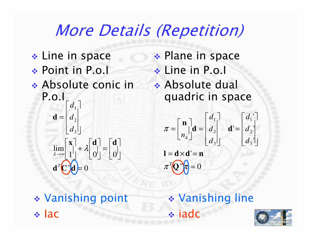
More Details (Repetition)

Line in space

Point in P.o.I

Absolute conic in P.o.I

Plane in space

Line in P.o.I

Absolute dual quadric in space

0

001lim

3

2

1

=

=

+

=

∞

∞→

dCd

ddx

d

T

d

d

d

λλ

0

'

'

'

'

'

3

2

1

3

2

1

4

=

=×=

=

=

=

∞ππ

π

Q

nddl

ddn

T

d

d

d

d

d

d

n

Vanishing point

Iac

Vanishing line

iadc

Why We Even Care? (2D version)

Because in 2D pole and polar relationship is projective invariant For point conic yyyyTTTTCxCxCxCx=0=0=0=0 For line conic mmmmTTTTCCCC*l=0*l=0*l=0*l=0

mmmm’’’’TTTTCCCC****’’’’llll’’’’=(H=(H=(H=(H----TTTTm)m)m)m)TTTTHCHCHCHC*H*H*H*HTTTT (H(H(H(H----TTTTllll)=)=)=)=mmmmTTTTCCCC*l*l*l*l

This means that known (orthogonal) directions in space Measured them in images (no longer orthogonal, but still satisfy pole-polar relationship)

Constraint on HHHH In regular Cartesian frame

C* C* C* C* is the absolute dual conic

In projective frame C*C*C*C*’’’’ is the image of absolute dual conic (iadc)

Angles In 2D Case

I, JI, JI, JI, J are circular points

Absolute dual conic is a degenerate conic (null space is line at infinity)

TT

T

TT

T

TT

T

C

ii

xxx

C

CC

C

dddddddd

dddd

JIIJ

JI

xx

dddd

dd

dddd

dd

+=

−==

==+

=

=

=

++

+=

∞

∞

∞∞

∞

*

3

2

2

2

1

*

2

*

21

*

1

2

*

1

2211

21

2222212112121111

22122111

)0,,1(),0,,1(

0,0

0

0

1

1

0

1

1

0

1

1

cosθ

Angles in 3D Case -Line

Absolute (point) conic is a conic on the plane at infinity

0,0

0

1

1

1

1

1

1

1

1

1

cos

4

2

3

2

2

2

1

2222

21

2211

21

232322222121131312121111

231322122111

==++⇒

=Ω⇒

ΩΩ

Ω=

=

++++

++=

∞

∞∞

∞

xxxx

dddddddddddd

dddddd

T

TT

T

TT

T

ll

llll

ll

llll

ll

θ

Angles in 3D Case -Plane

Absolute dual quadric is a degenerate quadric (null space is plane at infinity)

0,0

0

0

1

1

1

0

1

1

1

0

1

1

1

cos

4

2

3

2

2

2

1

*

2

*

22

*

2

2

*

1

2211

21

232322222121131312121111

231322122111

==++⇒

=⇒

=

=

++++

++=

∞

∞∞

∞

xxxx

Q

QQ

Q

dddddddddddd

dddddd

T

TT

T

TT

T

ππ

ππππ

ππ

ππππ

ππ

θ

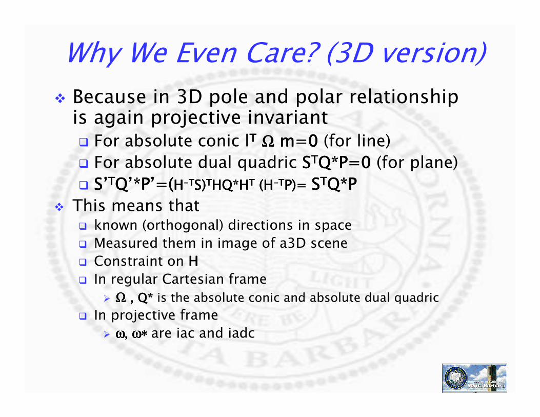
Why We Even Care? (3D version)

Because in 3D pole and polar relationship is again projective invariant For absolute conic lTTTT ΩΩΩΩ m=0 m=0 m=0 m=0 (for line)

For absolute dual quadric SSSSTTTTQ*P=0 Q*P=0 Q*P=0 Q*P=0 (for plane)

SSSS’’’’TTTTQQQQ’’’’*P*P*P*P’’’’=(=(=(=(HHHH----TTTTSSSS))))TTTTHQ*HHQ*HHQ*HHQ*HTTTT (H(H(H(H----TTTTP)P)P)P)= = = = SSSSTTTTQ*PQ*PQ*PQ*P

This means that known (orthogonal) directions in space

Measured them in image of a3D scene

Constraint on HHHH

In regular Cartesian frame

ΩΩΩΩ , Q* , Q* , Q* , Q* is the absolute conic and absolute dual quadric

In projective frame

ω, ω∗ ω, ω∗ ω, ω∗ ω, ω∗ are iac and iadc

Rectification

Rectification is a mathematic process of limiting DOFs of H H H H (camera or not)

If HHHH is to be decomposed further into camera matrix may not be considered (inner working of HHHH not recovered)

Cameras can be treated as a projective device

Affine camera

Induce affine transform

Perspective (pinhole) camera

Induce projective transform

Rectification Under Homography

Same camera center Different camera centers, but planar structure

Removing projective distortion #1

333231

131211

3

1

'

''

hyhxh

hyhxh

x

xx

++

++==

333231

232221

3

2

'

''

hyhxh

hyhxh

x

xy

++

++==

( ) 131211333231' hyhxhhyhxhx ++=++

( ) 232221333231' hyhxhhyhxhy ++=++

Select four points in a plane with know coordinates

(linear in hij)

(2 constraints/point, 8DOF ⇒ 4 points needed)

Remark: No camera calibration necessary

Overkill, from projective to similarity are only 4 DOFs away

Removing Projective Distortion #2

From projective to affine

Locate and move line of infinity

From affine to similarity

Locate and move circular points

2D Rectification Hierarchy From perspective to affine

HHHH preserves line of infinity if and only ifHHHH is affine

From affine to similarity

HHHH preserves absolute conic (or circular points) if and only if HHHH is similarity

0

0

1

0

0

'

'

0

0

0

1

0

)(

1

0

0

1

0

0

1')(

32

333231

232221

131211

31

333231

232221

131211

=→

=

=→

=

⇒

=

=

−==⇐ ∞−−

−

∞

−

∞

h

hhh

hhh

hhh

y

x

h

hhh

hhh

hhh

y

x

TT

T

T

A lAt

0AlHl

0vAA

vvAv

AvAA

t

vA

v

tA

C

t

0R

0

tRHCHC

==→

=

⇒

=

=

==⇐

,1

0

1

1

)(

*

0

1

1

10

1

1

1**')(

2

T

TTT

T

T

T

T

T

T

T

T

ss

vv

s

ss

Affine rectification

v1 v2

l1

l2 l4

l3

l∞

21 vvl ×=∞

211 llv ×=

432 llv ×=

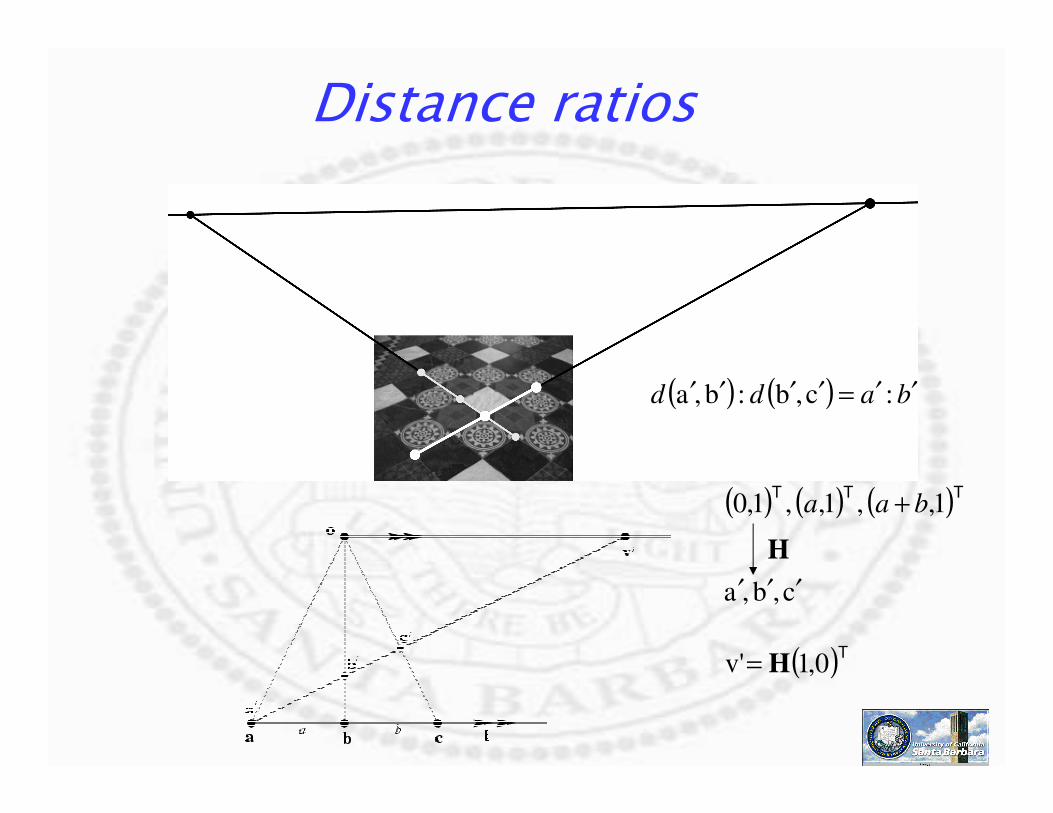
Distance ratios

( ) ( ) badd ′′=′′′′ :c,b:b,a

( )T0,1v' H=

( ) ( ) ( )TTT1,,1,,1,0 baa +

c,b,a ′′′

H

Metric from affine

( ) 000

0

3

2

1

321 =

′

′

′

′′′

m

m

m

lll

TKK

( )( ) 0,,,, 2

221211

2

12

2

1122122111 =+′′′′+′′′′T

kkkkkmlmlmlml

Image Formation

Specialization: camera is used as the projective device

Need to understand projection relationship of point, line, plane, conic, quadric, etc.

Need to dissect the camera matrix

Planar homography (discussed above) is a special case where 3D object is planar

Projective Relationship

Point

x=PXx=PXx=PXx=PX

X=X=X=X=PPPP++++xxxx (PPPP+=PPPPT(PPPPPPPPT)-1, PPPPPPPP+=I)

Line

Backprojection

π= PPPPTllll

((((xxxxTllll====0, (, (, (, (PX)PX)PX)PX)Tllll=0, =0, =0, =0, XXXXT ((((PPPPTllll)=0))=0))=0))=0)

[ ]

xKd

xKx

0

KxP

I0

K0K

IPP

1

11

1

0

−

−−

+

−

+

=

=

=

=

⇒

=

T

T

lKn

lKl

0

K

lP

T

T

T

T

T

=

=

=

=

0

π

More Projective Relationships

Point Conics Line Conics

Point Quadrics Plane Quadrics

Projection? Projection?Back-projection Envelop

Dual

Dual

Point Quadrics and Conics

Under the camera PPPP a conic CCCC back projects into a cone QQQQ= PPPPTTTTCP CP CP CP

Cone is a degenerate quadricCone is a degenerate quadricCone is a degenerate quadricCone is a degenerate quadric

Camera center is the null spaceCamera center is the null spaceCamera center is the null spaceCamera center is the null space

0)(

0)(

0)(

0

==

=⇒

=⇒

=

CCTT

TT

T

T

PCPCPP

XCPPX

CPXPX

Cxx

Plane Quadrics and Line Conics

Under the camera matrix P the outline of the quadric Q is the conic given by CCCC*=PQ*PPQ*PPQ*PPQ*PT

T

TT

TTT

TT

T

P*PQC

lP*PQl

lP*QlP

lPππ*Qπ

lCl

=⇒

=⇒

=⇒

==⇒

=

*

0)(

0)(

0

0*

Camera Calibration (cont.)

Why? Because we are interested in similaritysimilaritysimilaritysimilarityreconstruction xxxx =PXPXPXPX implies xxxx = (PHPHPHPH-1)(HXHXHXHX)

Even if we can perform reconstruction, the structure recovered is only up to HXHXHXHX (preserves co-linearity), which is not very useful

How does calibration help? xxxx =KR[I|0]X!= KR[I|0]HKR[I|0]X!= KR[I|0]HKR[I|0]X!= KR[I|0]HKR[I|0]X!= KR[I|0]H-1H XH XH XH X

If we know KKKK, you cannot fake R,R,R,R, except with another RRRR’’’’ (RHRHRHRH----1111 is not RRRR in general)

Reconstruction is similar to the original scene Angle, relative length can be measured

Proof

You can fool the camera (the same image and the same parameters) by

Using PHPHPHPH----1111 as projection matrix (with the same KKKK)

Using HXHXHXHX as the 3D scene

The matrix structure dictates similarity

]|'['

'

1

1

tRt'RRK0

t'Rt]|K[RPH

0

t'RH

PXt]X|K[Rx

λλ

λ

+=

=

=

==

−

−

T

T

Uncalibrated Camera

The same trick won’t work if you don’t know KKKK

M M M M has an RQ decomposition where

R R R R is upper triangular

QQQQ is orthogonal

RQMtCKRARK

]t|[RK

tRBtCRAKC

BAt]|K[RPH

C

BAH

PXt]X|K[Rx

==+=⇒

=

++=

=

=

==

−

T

T

T

T

''

'''

]|[1 λλ

λ

Camera Calibration (cont.)

Camera calibration does not give

Absolute scale

Absolute location

You cannot tell if you are flying over New York City or flying over a model of New York City in Santa Barbara

The best you can hope for with a single camera with no object of known scale

Camera Calibration

There are two components

Intrinsic parameters: independent of placement, dependent on camera used

Extrinsic parameters: dependent on placement, independent of camera used

Projective geometry constraint is on intrinsic parameters only

Other constraints have to be brought in to determine placement

Dissecting Camera Matrix

x=PX

RCTPCIKR

PTRK

Pr

r

r

PTR

p

3

2

1

−=−=

=

=

=

world

world

world

z

y

x

ov

ou

worldov

ou

real

t

t

t

vk

uk

vk

uk

]|[

]|[

100100

0010

0001

100

0

100100

0010

0001

100

0

α

α

More Simplification

In a camera-centered coordinate frame

RRRR is identity

CCCC is (0,0,0)

PPPP= KRKRKRKR[IIII|-CCCC] =KKKK[IIII|0000]

For affine camera, the camera center is at infinity and the focal length increase to infinity

PPPP becomes an affine matrix

3D Rectification Hierarchy From perspective to affine

HHHH preserves plane of infinity if and only ifHHHH is affine

From affine to similarity

HHHH preserves absolute conic (or absolute dual quadric) if and only if HHHHis similarity

0

0

0

0

0

1

0

)(

1

0

0

0

1

0

0

0

1')(

3332

31

44434241

34333231

24232221

14131211

==→

=→

=

⇒

=

=

−==⇐ ∞−−

−

∞

−

∞

hh

h

hhhh

hhhh

hhhh

hhhh

y

x

TT

T

T

A lAt

0AlHl

0vAA

vvAv

AvAA

t

vA

v

tA

Q

t

0R

0

tRHQHC

==→

=

⇒

=

=

==⇐

∞

∞

,1

0

1

1

1

)(

0

1

1

1

1

0

1

1

1

1*')(

*2

*

T

TTT

T

T

T

T

T

T

T

T

ss

kv

s

ss

More Details (Repetition)

Line in space

Point in P.o.I

Absolute conic in P.o.I

Plane in space

Line in P.o.I

Absolute dual quadric in space

0

001lim

3

2

1

=

=

+

=

∞

∞→

dCd

ddx

d

T

d

d

d

λλ

0

'

'

'

'

'

3

2

1

3

2

1

4

=

=×=

=

=

=

∞ππ

π

Q

nddl

ddn

T

d

d

d

d

d

d

n

Vanishing point

Iac

Vanishing line

iadc

More Details (Repetition)

0

0)()(

0

001lim

1

11

3

2

1

=

=

=

=

+

=

−−

−∞−

∞

∞→

xKKx

xKCxK

dCd

ddx

d

TT

T

T

d

d

d

λλ

[ ] 00

0

'

'

'

'

'

4

4

3

2

1

3

2

1

4

==

=

=×=

=

=

=

∞

lKKllK

0

0IKl

Q

nddl

ddn

TT

T

T

T

T

nn

d

d

d

d

d

d

n

ππ

π

Vanishing point

Iac

Vanishing line

iadc

Comparison

2D planar homography Plane to plane correspondence

Move line of infinity

Recover circular point

Similarity

3D planar homography

Image plane and plane at infinity correspondence

?

Recover absolute conic and dual absoluate conic

Similarity (determining intrinsic parameters)

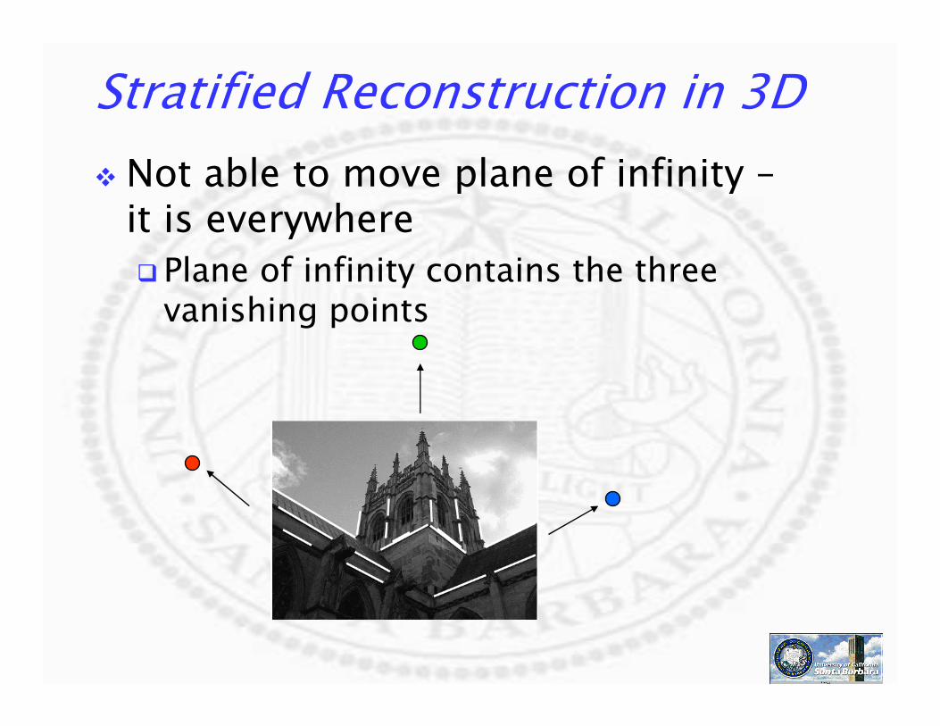
Stratified Reconstruction in 3D

Not able to move plane of infinity –it is everywhere

Plane of infinity contains the three vanishing points

Stratified Reconstruction in 3D

Parallel lines (of a single direction) on parallel planes have a single vanishing point (point at infinity)

Different sets of parallel lines (of multiple directions) on parallel planes have vanishing points on a single vanishing line (line at infinity)

Multiple sets of parallel planes (of multiple directions) have multiple vanishing lines (plane at infinity)

Measuring Directions Using camera

For image points For image lines

C x1

x2

d1

d2

θ

xKd

Kd

d0IK

dCPx

1

)01

](0|[

)01

(

−=

→=

+

=

+

=

λ

λ

C

x

d=K-1x

ln=KTl

lKn

lnK

nKx

nxK

ndlx

T

T

TT

T

TT

=⇒

=⇒

=⇒

=⇒

==

−

−

−

0)(

0)(

0,0

1

An Important Homography Relation

Images of plane at infinity and image plane form a planar homography

HdKRdd

CIKRXx ==

−== ∞

0]|[P

Projection of AC and ADQ

Image of absolute conic (iac)

Image of absolute dual quadric (iadc)

TTT

TT

TT

TT

KKKKRR

KRC

I

00

0IC|IKR

KKKRIKR

PPQHCH

==

−

−=

==

=→

−−−

∞

−

∞

−

][)()()( 11

**1

ω

ωω

If iac or idac can be recovered, camera can be calibrated

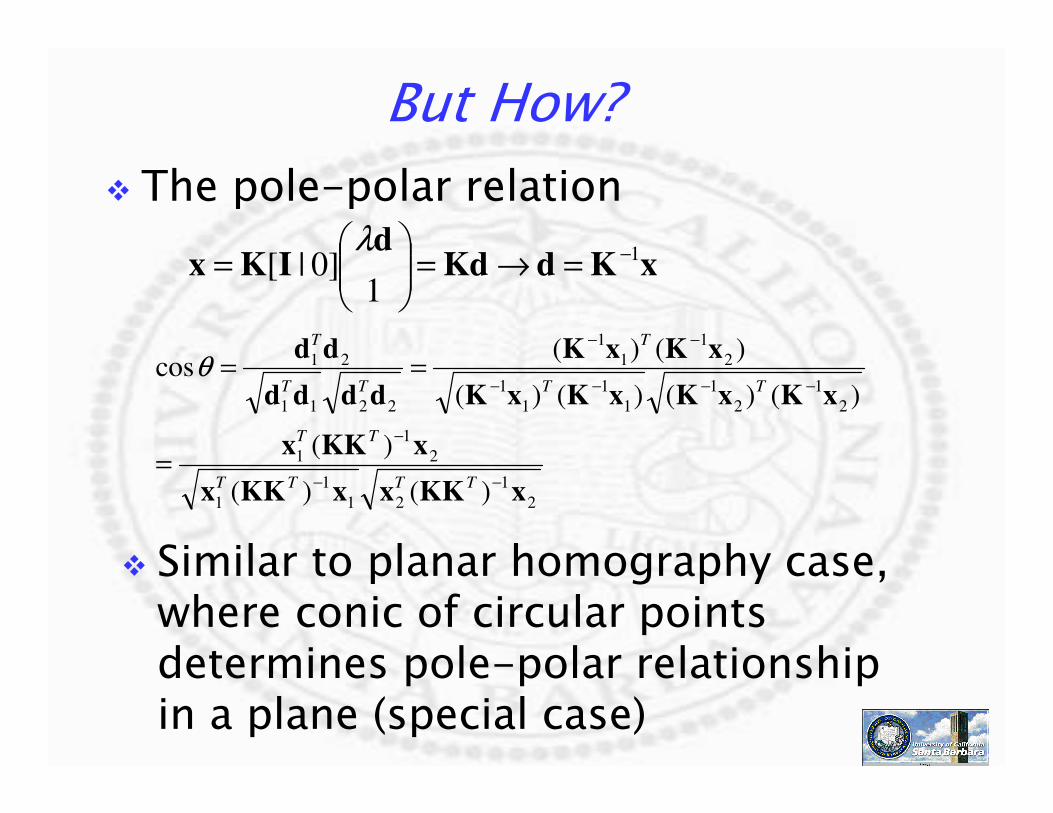
But How?

The pole-polar relation

xKdKdd

IKx 1

1]0|[ −=→=

=

λ

2

1

21

1

1

2

1

1

2

1

2

1

1

1

1

1

2

1

1

1

2211

21

)()(

)(

)()()()(

)()(cos

xKKxxKKx

xKKx

xKxKxKxK

xKxK

dddd

dd

−−

−

−−−−

−−

=

==

TTTT

TT

TT

T

TT

T

θ

Similar to planar homography case, where conic of circular points determines pole-polar relationship in a plane (special case)

General Procedure

Measure 2D image points (x1, x2x1, x2x1, x2x1, x2)

Relate that to 3D direction (d1, d2d1, d2d1, d2d1, d2)

Impose constraints on θ (e.g., some directions are orthogonal)

But how do we know two directions are perpendicular?

C x1

x2

d1

d2

θ

Yet Another Dual Relation

Vanishing point

Images of lines

Invariant measure using AC

Vanishing line

Images of planes

Invariant measure using IAC

point vanishing

)()()(,

0

111

21

→

==→

=

−−−−

∞

−

∞

d

KKKRIKRωHCHω

dCd

TTT

T

line anishing

][,

0

***

2

*

1

v

TTT

TTT

T

→

==

−

−=→

=

∞

∞

π

KKKKRR

KRC

I

00

0IC|IKRPPQω

πQπ

ω

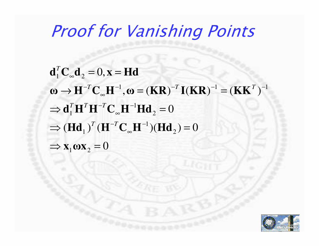
Proof for Vanishing Points

0

0))(()(

0

)()()(,

,0

21

2

1

1

2

1

1

111

21

=⇒

=⇒

=⇒

==→

==

−

∞

−

−

∞

−

−−−−

∞

−

∞

ωxx

HdHCHHd

HdHCHHd

KKKRIKRωHCHω

HdxdCd

TT

TTT

TTT

T

Proof for Vanishing Lines

[ ]

[ ]

0

0

01

1

01

1

][,

,0

2

*

1

21

2

T

1

2

1

***

T

2

*

1

=⇒

=⇒

=

⇒

=

⇒

==

−

−=→

==

∞

∞

lωl

lKKl

lK

00

0IKl

n

00

0In

KKKKRR

KRC

I

00

0IC|IKRPPQω

lKnπQπ

T

T

TTT

TTT

T

ω

( ) ( ) λKdaλPDPAλPXλx +=+==

( ) ( ) KdλKda limλ xlimvλλ

=+==∞→∞→

KdPXv == ∞

Vanishing points

Vanishing lines

Vanishing Points and Vanishing Lines

If you can locate vanishing points and lines in images, then you can know their 3D directions (in camera’s coordinate system)

Using domain knowledge you can impose constraints on KKKK

A Hybrid Relation

For a line and a plane in space

We have a point (x) and a line (l) in image

l=l=l=l=wxwxwxwx, x=w*l , x=w*l , x=w*l , x=w*l if they are orthogonal

Proof left as an exercise

compute H for each square

(corners (0,0),(1,0),(0,1),(1,1))

compute the imaged circular points H(1,±i,0)T

fit a conic to 6 circular points

compute KKKK from wwww through Cholesky factorization

Using Homography

Using Other Relationships

Image plane

Two vanishing points

1 vanishing point + 1 vanishing line

Plane

3D space

Two orthogonal lines

Orthogonal line and plane

Plane